A class of measure-valued Markov chains and Bayesian nonparametrics

Abstract

Measure-valued Markov chains have raised interest in Bayesian nonparametrics since the seminal paper by (Math. Proc. Cambridge Philos. Soc. 105 (1989) 579–585) where a Markov chain having the law of the Dirichlet process as unique invariant measure has been introduced. In the present paper, we propose and investigate a new class of measure-valued Markov chains defined via exchangeable sequences of random variables. Asymptotic properties for this new class are derived and applications related to Bayesian nonparametric mixture modeling, and to a generalization of the Markov chain proposed by (Math. Proc. Cambridge Philos. Soc. 105 (1989) 579–585), are discussed. These results and their applications highlight once again the interplay between Bayesian nonparametrics and the theory of measure-valued Markov chains.

, and

1 Introduction

Measure-valued Markov chains, or more generally measure-valued Markov processes, arise naturally in modeling the composition of evolving populations and play an important role in a variety of research areas such as population genetics and bioinformatics (see, e.g., [10, 9, 26, 5]), Bayesian nonparametrics [38, 31], combinatorics [26] and statistical physics [26, 5, 6]. In particular, in Bayesian nonparametrics there has been interest in measure-valued Markov chains since the seminal paper by [12], where the law of the Dirichlet process has been characterized as the unique invariant measure of a certain measure-valued Markov chain.

In order to introduce the result by [12], let us consider a Polish space $\mathbb{X}$ endowed with the Borel $\sigma$-field $\mathscr{X}$ and let $\mathcal{P}_{\mathbb{X}}$ be the space of probability measures on $\mathbb{X}$ with the $\sigma$-field $\mathscr{P}_{\mathbb{X}}$ generated by the topology of weak convergence. If $\alpha$ is a strictly positive finite measure on $\mathbb{X}$ with total mass $a>0$, $Y$ is a $\mathbb{X}$-valued random variable (r.v.) distributed according to $\alpha_{0}:=\alpha/a$ and $\theta$ is a r.v. independent of $Y$ and distributed according to a Beta distribution with parameter $(1,a)$ then, Theorem 3.4 in [33] implies that a Dirichlet process $P$ on $\mathbb{X}$ with parameter $\alpha$ uniquely satisfies the distributional equation

$$P\stackrel{{\scriptstyle\mathrm{d}}}{{=}}\theta\delta_{Y}+(1-\theta)P,$$ (1)

where all the random elements on the right-hand side of (1) are independent. All the r.v.s introduced in this paper are meant to be assigned on a probability space $(\Omega,\mathscr{F},\mathbb{P})$ unless otherwise stated. In [12], (1) is recognized as the distributional equation for the unique invariant measure of a measure-valued Markov chain $\{P_{m},m\geq 0\}$ defined via the recursive identity

$$P_{m}=\theta_{m}\delta_{Y_{m}}+(1-\theta_{m})P_{m-1},\qquad m\geq 1,$$ (2)

where $P_{0}\in\mathcal{P}_{\mathbb{X}}$ is arbitrary, $\{Y_{m},m\geq 1\}$ is a sequence of $\mathbb{X}$-valued r.v.s independent and identically distributed as $Y$ and $\{\theta_{m},m\geq 1\}$ is a sequence of r.v.s, independent and identically distributed as $\theta$ and independent of $\{Y_{m},m\geq 1\}$. We term $\{P_{m},m\geq 0\}$ as the Feigin–Tweedie Markov chain. By investigating the functional Markov chain $\{G_{m},m\geq 0\}$, with $G_{m}:=\int_{\mathbb{X}}g(x)P_{m}(\mathrm{d}x)$ for any $m\geq 0$ and for any measurable linear function $g\mathchoice{\nobreak\,\colon}{\nobreak\,\colon}{\nobreak\,\colon\;}{\nobreak\,\colon\;}\mathbb{X}\mapsto\mathbb{R}$, [12] provide properties of the corresponding linear functional of a Dirichlet process. In particular, the existence of the linear functional $G:=\int_{\mathbb{X}}g(x)P(\mathrm{d}x)$ of the Dirichlet process $P$ is characterized according to the condition $\int_{\mathbb{X}}\log(1+|g(x)|)\alpha(\mathrm{d}x)<+\infty$; these functionals were considered by [16] and their existence was also investigated by [7] who referred to them as moments, as well as by [39] and [4]. Further developments of the linear functional Markov chain $\{G_{m},m\geq 0\}$ are provided by [15, 17] and more recently by [8].

Starting from the distributional equation (1), a constructive definition of the Dirichlet process has been proposed by [33]. If $P$ is a Dirichlet process on $\mathbb{X}$ with parameter $\alpha=a\alpha_{0}$, then $P=\sum_{1\leq i\leq\infty}p_{i}\delta_{Y_{i}}$ where $\{Y_{i},i\geq 1\}$ is a sequence of independent r.v.s identically distributed according to $\alpha_{0}$ and $\{p_{i},i\geq 1\}$ is a sequence of r.v.s independent of $\{Y_{i},i\geq 1\}$ and derived by the so-called stick breaking construction, that is, $p_{1}=w_{1}$ and $p_{i}=w_{i}\prod_{1\leq j\leq i-1}(1-w_{j})$ for $i>1$, with $\{w_{i},i\geq 1\}$ being a sequence of independent r.v.s identically distributed according to a Beta distribution with parameter $(1,a)$. Then, equation (1) arises by considering

$$P=p_{1}\delta_{Y_{1}}+(1-w_{1})\sum_{i=2}^{\infty}\tilde{p}_{i}\delta_{Y_{i}},$$

where now $\tilde{p}_{2}=w_{2}$ and $\tilde{p}_{i}=w_{i}\prod_{2\leq j\leq i-1}(1-w_{j})$ for $i>2$. Thus, it is easy to see that $\tilde{P}:=\sum_{2\leq i\leq\infty}\tilde{p}_{i}\delta_{Y_{i}}$ is also a Dirichlet process on $\mathbb{X}$ with parameter $\alpha$ and it is independent of the pairs of r.v.s $(p_{1},Y_{1})$. If we would extend this idea to $n$ initial samples, we should consider writing

$$P=\theta\sum_{i=1}^{n}\biggl{(}\frac{p_{i}}{\theta}\biggr{)}\delta_{Y_{i}}+(1-\theta)\tilde{P},$$

where $\theta=\sum_{1\leq i\leq n}p_{i}=1-\prod_{1\leq i\leq n}(1-w_{i})$ and $\tilde{P}$ is a Dirichlet process on $\mathbb{X}$ with parameter $\alpha$ independent of the random vectors $(p_{1},\ldots,p_{n})$ and $(Y_{1},\ldots,Y_{n})$. However, this is not an easy extension since the distribution of $\theta$ is unclear, and moreover $\theta$ and $\sum_{1\leq i\leq n}(p_{i}/\theta)\delta_{Y_{i}}$ are not independent. For this reason, in [11] an alternative distributional equation has been introduced. Let $\alpha$ be a strictly positive finite measure on $\mathbb{X}$ with total mass $a>0$ and let $\{Y_{j},j\geq 1\}$ be a $\mathbb{X}$-valued Pólya sequence with parameter $\alpha$ (see [2]), that is, $\{Y_{j},j\geq 1\}$ is a sequence of $\mathbb{X}$-valued r.v.s characterized by the following predictive distributions

$$\mathbb{P}(Y_{j+1}\in A|Y_{1},\ldots,Y_{j})=\frac{1}{a+j}\alpha(A)+\frac{1}{a+j}\sum_{i=1}^{j}\delta_{Y_{i}}(A),\qquad j\geq 1,$$

and $\mathbb{P}(Y_{1}\in A)=\alpha(A)/a$, for any $A\in\mathscr{X}$. The sequence $\{Y_{j},j\geq 1\}$ is exchangeable, that is, for any $j\geq 1$ and any permutation $\sigma$ of the indexes $(1,\ldots,j)$, the law of the r.v.s $(Y_{1},\ldots,Y_{j})$ and $(Y_{\sigma(1)},\ldots,Y_{\sigma(j)})$ coincide; in particular, according to the celebrated de Finetti representation theorem, the Pólya sequence $\{Y_{j},j\geq 1\}$ is characterized by a so-called de Finetti measure, which is the law of a Dirichlet process on $\mathbb{X}$ with parameter $\alpha$. For a fixed integer $n\geq 1$, let $(q_{1}^{(n)},\ldots,q_{n}^{(n)})$ be a random vector distributed according to the Dirichlet distribution with parameter $(1,\ldots,1)$, $\sum_{1\leq i\leq n}q_{i}^{(n)}=1$, and let $\theta$ be a r.v. distributed according to a Beta distribution with parameter $(n,a)$ such that $\{Y_{i},i\geq 1\}$, $(q^{(n)}_{1},\ldots,q^{(n)}_{n})$ and $\theta$ are mutually independent. Moving from such a collection of random elements, Lemma 1 in [11] implies that a Dirichlet process $P^{(n)}$ on $\mathbb{X}$ with parameter $\alpha$ uniquely satisfy the distributional equation

$$P^{(n)}\stackrel{{\scriptstyle\mathrm{d}}}{{=}}\theta\sum_{i=1}^{n}q_{i}^{(n)}\delta_{Y_{i}}+(1-\theta)P^{(n)},$$ (3)

where all the random elements on the right-hand side of (3) are independent. In order to emphasize the additional parameter $n$, we used an upper-script $(n)$ on the Dirichlet process $P$ and on the random vector $(q_{1}^{(n)},\ldots,q_{n}^{(n)})$. It can be easily checked that equation (3) generalizes (1), which can be recovered by setting $n=1$.

In the present paper, our aim is to further investigate the distributional equation (3) and its implications in Bayesian nonparametrics theory and methods. The first part of the paper is devoted to investigate the random element $\sum_{1\leq i\leq n}q_{i}^{(n)}\delta_{Y_{i}}$ in (3) which is recognized to be the random probability measure (r.p.m.) at the $n$th step of a measure-valued Markov chain defined via the recursive identity

$$\sum_{i=1}^{n}q_{i}^{(n)}\delta_{Y_{i}}=W_{n}\delta_{Y_{n}}+(1-W_{n})\sum_{i=1}^{n-1}q_{i}^{(n-1)}\delta_{Y_{i}},\qquad n\geq 1,$$ (4)

where $\{W_{n},n\geq 1\}$ is a sequence of independent r.v.s, each $W_{n}$ distributed according a Beta distribution with parameter $(1,n-1)$, $q_{i}^{(n)}=W_{i}\prod_{i+1\leq j\leq n}(1-W_{j})$ for $i=1,\ldots,n$ and $n\geq 1$ and the sequence $\{W_{n},n\geq 1\}$ is independent from $\{Y_{n},n\geq 1\}$. More generally, we observe that the measure-valued Markov chain defined via the recursive identity (4) can be extended by considering, instead of a Pólya sequence $\{Y_{n},n\geq 1\}$ with parameter $\alpha$, any exchangeable sequence $\{Z_{n},n\geq 1\}$ characterized by some de Finetti measure on $\mathcal{P}_{\mathbb{X}}$ and such that $\{W_{n},n\geq 1\}$ is independent from $\{Z_{n},n\geq 1\}$. Asymptotic properties for this new class of measure-valued Markov chains are derived and some linkages to Bayesian nonparametric mixture modelling are discussed. In particular, we remark how it is closely related to a well-known recursive algorithm introduced in [25] for estimating the underlying mixing distribution in mixture models, the so-called Newton’s algorithm.

In the second part of the paper, by using finite and asymptotic properties of the r.p.m. $\sum_{1\leq i\leq n}q_{i}^{(n)}\delta_{Y_{i}}$ and by following the original idea of [12], we define and investigate from (3) a class of measure-valued Markov chain $\{P^{(n)}_{m},m\geq 0\}$ which generalizes the Feigin–Tweedie Markov chain, introducing a fixed integer parameter $n$. Our aim is in providing features of the Markov chain $\{P^{(n)}_{m},m\geq 0\}$ in order to verify if it preserves some of the properties characterizing the Feigin–Tweedie Markov chain; furthermore, we are interested in analyzing asymptotic (as $m$ goes to $+\infty$) properties of the associated linear functional Markov chain $\{G^{(n)}_{m},m\geq 0\}$ with $G^{(n)}_{m}:=\int_{\mathbb{X}}g(x)P^{(n)}_{m}(\mathrm{d}x)$ for any $m\geq 0$ and for any function $g\mathchoice{\nobreak\,\colon}{\nobreak\,\colon}{\nobreak\,\colon\;}{\nobreak\,\colon\;}\mathbb{X}\mapsto\mathbb{R}$ such that $\int_{\mathbb{R}}\log(1+|g(x)|)\alpha(\mathrm{d}x)<+\infty$. In particular, we show that the Feigin–Tweedie Markov chain $\{P_{m},m\geq 0\}$ sits in a larger class of measure-valued Markov chains $\{P^{(n)}_{m},m\geq 0\}$ parametrized by an integer number $n$ and still having the law of a Dirichlet process with parameter $\alpha$ as unique invariant measure. The role of the further parameter $n$ is discussed in terms of new potential applications of the Markov chain $\{P^{(n)}_{m},m\geq 0\}$ with respect to the the known applications of the Feigin–Tweedie Markov chain.

Following these guidelines, in Section 2 we introduce a new class of measure-valued Markov chains $\{Q_{n},n\geq 1\}$ defined via exchangeable sequences of r.v.s; asymptotic results for $\{Q_{n},n\geq 1\}$ are derived and applications related to Bayesian nonparametric mixture modelling are discussed. In Section 3, we show that the Feigin–Tweedie Markov chain $\{P_{m},m\geq 0\}$ sits in a larger class of measure-valued Markov chains $\{P^{(n)}_{m},m\geq 0\}$, which is investigated in comparison with $\{P_{m},m\geq 0\}$. In Section 4, some concluding remarks and future research lines are presented.

2 A class of measure-valued Markov chains and Newton’s algorithm

Let $\{W_{n},n\geq 1\}$ be a sequence of independent r.v.s such that $W_{1}=1$ almost surely and $W_{n}$ has Beta distribution with parameter $(1,n-1)$ for $n\geq 2$. Moreover, let $\{Z_{n},n\geq 1\}$ be a sequence of $\mathbb{X}$-valued exchangeable r.v.s independent from $\{W_{n},n\geq 1\}$ and characterized by some de Finetti measure on $\mathcal{P}_{\mathbb{X}}$. Let us consider the measure-valued Markov chain $\{Q_{n},n\geq 1\}$ defined via the recursive identity

$$Q_{n}=W_{n}\delta_{Z_{n}}+(1-W_{n})Q_{n-1},\qquad n\geq 1.$$ (5)

In the next theorem, we provide an alternative representation of $Q_{n}$ and show that $Q_{n}(\omega)$ converges weakly to some limit probability $Q(\omega)$ for almost all $\omega\in\Omega$, that is, for each $\omega$ in some set $A\in\mathscr{F}$ with $\mathbb{P}(A)=1$. In short, we use notation $Q_{n}\Rightarrow Q$ a.s.-$\mathbb{P}$.

Theorem 1

Let $\{Q_{n},n\geq 1\}$ be the Markov chain defined by (5). Then:

1. [(ii)]

2. an equivalent representation of $Q_{n}$, $n=1,2,\ldots$ is

   $$Q_{n}=\sum_{i=1}^{n}q_{i}^{(n)}\delta_{Z_{i}},$$ (6)

   where $\sum_{1\leq i\leq n}q_{i}^{(n)}=1$, $q^{(n)}=(q^{(n)}_{1},\ldots,q^{(n)}_{n})$ has Dirichlet distribution with parameter $(1,1,\ldots,1)$, and $\{q^{(n)},n\geq 1\}$ and $\{Z_{n},n\geq 1\}$ are independent.

3. There exists a r.p.m. $Q$ on $(\Omega,\mathscr{F},\mathbb{P})$ such that, as $n\rightarrow+\infty$,

   $$Q_{n}\Rightarrow Q,\qquad\mbox{{a.s.}-}\mathbb{P},$$

   where the law of $Q$ is the de Finetti measure of the sequence $\{Z_{n},n\geq 1\}$.

Proof.

As far as (i) is concerned, by repeated application of the recursive identity (5), it can be checked that, for any $n\geq 1$,

$$Q_{n}=\sum_{i=1}^{n}W_{i}\prod_{j=i+1}^{n}(1-W_{j})\delta_{Z_{i}},$$

where $W_{1}=1$ almost surely and $\prod_{i+1\leq j\leq n}(1-W_{j})$ is defined to be 1 when $i=n$. Defining $q_{i}^{(n)}:=W_{i}\prod_{i+1\leq j\leq n}(1-W_{j})$, $i=1,\ldots,n$, it is straightforward to show that $q^{(n)}=(q^{(n)}_{1},\ldots,q^{(n)}_{n})$ has the Dirichlet distribution with parameter $(1,1,\ldots,1)$ and $\sum_{1\leq i\leq n}q_{i}^{(n)}=1$, so that (6) holds.

Regarding (ii), by the definition of the Dirichlet distribution, an equivalent representation of (6) is

$$Q_{n}=\sum_{i=1}^{n}q_{i}^{(n)}\delta_{Z_{i}}=\sum_{i=1}^{n}\frac{\lambda_{i}}{\sum_{j=1}^{n}\lambda_{j}}\delta_{Z_{i}},$$

where $\{\lambda_{n},n\geq 1\}$ is a sequence of r.v.s independent and identically distributed according to standard exponential distribution, independent from $\{Z_{n},n\geq 1\}$. Let $g\mathchoice{\nobreak\,\colon}{\nobreak\,\colon}{\nobreak\,\colon\;}{\nobreak\,\colon\;}\mathbb{X}\rightarrow\mathbb{R}$ be any bounded continuous function, and consider

$$G_{n}=\int_{\mathbb{X}}g\,\mathrm{d}Q_{n}=\sum_{i=1}^{n}\frac{\lambda_{i}}{\sum_{1}^{n}\lambda_{j}}g(Z_{i})=\frac{{\sum_{i=1}^{n}\lambda_{i}g(Z_{i})}/n}{{\sum_{1}^{n}\lambda_{i}}/n}.$$

The expression in the denominator converges almost surely to 1 by the strong law of large numbers. As far as the numerator is concerned, let $Q$ be the r.p.m. defined on $(\Omega,\mathscr{F},\mathbb{P})$, such that the r.v.s $\{Z_{n},n\geq 1\}$ are independent and identically distributed conditionally on $Q$; the existence of such a random element is guaranteed by the de Finetti representation theorem (see, e.g., [32], Theorem 1.49). It can be shown that $\{\lambda_{n}g(Z_{n}),n\geq 1\}$ is a sequence of exchangeable r.v.s and, if $t_{1},\ldots,t_{n}\in\mathbb{R}$,

$$\mathbb{P}\bigl{(}\lambda_{1}g(Z_{1})\leq t_{1},\ldots,\lambda_{n}g(Z_{n})\leq t_{n}\bigr{)}$$

$$\quad=\int_{(0,+\infty)^{n}}\mathbb{P}\bigl{(}\lambda_{1}g(Z_{1})\leq t_{1},\ldots,\lambda_{n}g(Z_{n})\leq t_{n}|\lambda_{1},\ldots,\lambda_{n}\bigr{)}\prod_{i=1}^{n}\e^{-\lambda_{i}}\,\mathrm{d}\lambda_{i}$$

$$\quad=\int_{(0,+\infty)^{n}}\int_{{\mathcal{P}}_{\mathbb{R}}}\prod_{i=1}^{n}F_{Q^{*}}\biggl{(}\frac{t_{i}}{\lambda_{i}}\biggr{)}\mu(\mathrm{d}Q^{*})\prod_{i=1}^{n}\e^{-\lambda_{i}}\,\mathrm{d}\lambda_{i}$$

$$\quad=\int_{\mathcal{P}_{\mathbb{R}}}\prod_{i=1}^{n}\biggl{(}\int_{0}^{+\infty}F_{Q^{*}}\biggl{(}\frac{t_{i}}{\lambda_{i}}\biggr{)}\e^{-\lambda_{i}}\,\mathrm{d}\lambda_{i}\biggr{)}\mu(\mathrm{d}Q^{*}),$$

where $Q^{*}(A,\omega):=P(g^{-1}(A),\omega)$, $\omega\in\Omega$, $A\in\mathscr{R}$, is a r.p.m. with trajectories in ${\mathcal{P}_{\mathbb{R}}}$, and $F_{Q^{*}}$ denotes the random distribution relative to $Q^{*}$. This means that, conditionally on $Q^{*}$, $\{\lambda_{n}g(Z_{n}),n\geq 1\}$ is a sequence of r.v.s independent and identically distributed according to the random distribution (evaluated in $t$)

$$\int_{0}^{+\infty}F_{Q^{*}}\biggl{(}\frac{t}{y}\biggr{)}\e^{-y}\,\mathrm{d}y.$$

Of course, $\mathbb{E}|\lambda_{1}g(Z_{1})|=\mathbb{E}(\lambda_{1})\mathbb{E}|g(Z_{1})|<+\infty$ since $g$ is bounded. As in [3], Example 7.3.1, this condition implies

$$\frac{1}{n}\sum_{i=1}^{n}\lambda_{i}g(Z_{i}) \stackrel{{\scriptstyle\mathrm{a.s.}}}{{\rightarrow}} \mathbb{E}(\lambda_{1}g(Z_{1})|Q^{*})=\int_{\mathbb{R}}t\,\mathrm{d}\biggl{(}\int_{0}^{+\infty}F_{Q^{*}}\biggl{(}\frac{t}{y}\biggr{)}\e^{-y}\,\mathrm{d}y\biggr{)}$$

$$= \int_{\mathbb{R}}uQ^{*}(\mathrm{d}u)=\int_{\mathbb{X}}g(x)Q(\mathrm{d}x),$$

so that $G_{n}\rightarrow\int_{\mathbb{X}}g(x)Q(\mathrm{d}x)$ a.s.-$\mathbb{P}$. By Theorem 2.2 in [1], it follows that $Q_{n}\Rightarrow Q$ a.s.-$\mathbb{P}$ as $n\rightarrow+\infty$. ∎

Throughout the paper, $\alpha$ denotes a strictly positive and finite measure on $\mathbb{X}$ with total mass $a$, unless otherwise stated. If the exchangeable sequence $\{Z_{n},n\geq 1\}$ is the Pólya sequence with parameter $\alpha$, then by Theorem 1(i) $\{Q_{n},n\geq 1\}$ is the Markov chain defined via the recursive identity (4); in particular, by Theorem 1(ii), $Q_{n}\Rightarrow Q$ $\mathrm{a.s.\mbox{-}}\mathbb{P}$ where $Q$ is a Dirichlet process on $\mathbb{X}$ with parameter $\alpha$. This means that, for any fixed integer $n\geq 1$, the r.p.m. $Q_{n}$ can be interpreted as an approximation of a Dirichlet process with parameter $\alpha$. In Appendix .1, we present an alternative proof of the weak convergence (convergence of the finite dimensional distribution) of $\{Q_{n},n\geq 1\}$ to a Dirichlet process on $\mathbb{X}$ with parameter $\alpha$, using a combinatorial technique. As a byproduct of this proof, we obtain an explicit expression for the moment of order $(r_{1},\ldots,r_{k}$) of the $k$-dimensional Pólya distribution.

A straightforward generalization of the Markov chain $\{Q_{n},n\geq 0\}$ can be obtained by considering a nonparametric hierarchical mixture model. Let $k\mathchoice{\nobreak\,\colon}{\nobreak\,\colon}{\nobreak\,\colon\;}{\nobreak\,\colon\;}\mathbb{X}\times\Theta\rightarrow\mathbb{R}^{+}$ be a kernel, that is, $k(x,\vartheta)$ is a measurable function such that $x\mapsto k(x,\vartheta)$ is a density with respect to some $\sigma$-finite measure $\lambda$ on $\mathbb{X}$, for any fixed $\vartheta\in\Theta$, where $\Theta$ is a Polish space (with the usual Borel $\sigma$-field). Let $\{Q_{n},n\geq 1\}$ be the Markov chain defined via (5). Then for each $x\in\mathbb{X}$ we introduce a real-valued Markov chain $\{f^{(Q)}_{n}(x),n\geq 1\}$ defined via the recursive identity

$$f^{(Q)}_{n}(x)=W_{n}k(x,\vartheta_{n})+(1-W_{n})f^{(Q)}_{n-1}(x),\qquad n\geq 1,$$ (7)

where

$$f^{(Q)}_{n}(x)=\int_{\Theta}k(x,\vartheta)Q_{n}(\mathrm{d}\vartheta).$$

By a straightforward application of Theorem 2.2 in [1], for any fixed $x\in\mathbb{X}$, when $\vartheta\mapsto k(x,\vartheta)$ is continuous for all $x\in\mathbb{X}$ and bounded by a function $h(x)$, as $n\rightarrow+\infty$, then

$$f^{(Q)}_{n}(x)\rightarrow f^{(Q)}(x):=\int_{\Theta}k(x,\vartheta)Q(\mathrm{d}\vartheta),\qquad\mathrm{a.s.\mbox{-}}\mathbb{P},$$ (8)

where $Q$ is the limit r.p.m. in Theorem 1. For instance, if $Q$ is a Dirichlet process on $\mathbb{X}$ with parameter $\alpha$, $f^{(Q)}$ is precisely the density in the Dirichlet process mixture model introduced by [19]. When $h(x)$ is a $\lambda$-integrable function, not only the limit $f^{Q}(x)$ is a random density, but a stronger result than (8) is achieved.

Theorem 2

If $\vartheta\mapsto k(x,\vartheta)$ is continuous for all $x\in\mathbb{X}$ and bounded by a $\lambda$-integrable function $h(x)$, then

$$\lim_{n\rightarrow+\infty}\int_{\mathbb{X}}\bigl{|}f^{(Q)}_{n}(x)-f^{(Q)}(x)\bigr{|}\lambda(\mathrm{d}x)\rightarrow 0,\qquad\mathrm{a.s.\mbox{-}}\mathbb{P},$$

where $Q$ is the limit r.p.m. in Theorem 1.

Proof.

The functions $f^{(Q)}_{n}$ and $f^{(Q)}(x)=\int_{\Theta}k(x,\vartheta)Q(\mathrm{d}\vartheta)$, defined on $\mathbb{X}\times\Omega$, are $\mathscr{X}\otimes\mathscr{F}$-measurable, by a monotone class argument. In fact, by kernel’s definition, $(x,\vartheta)\mapsto k(x,\vartheta)$ is $\mathscr{X}\otimes\mathcal{B}(\Theta)$-measurable. Moreover, if $k=\mathbbl{1}_{A}\mathbbl{1}_{B}$, $A\in\mathscr{X}$ and $B\in\mathcal{B}(\Theta)$, then

$$f^{(Q)}(x,\omega)=\int k(x,\vartheta)Q(\mathrm{d}\vartheta;\omega)=\mathbbl{1}_{A}(x)Q(B;\omega)$$

is $\mathscr{X}\otimes\mathscr{F}$-measurable. Let ${\mathcal{C}}=\{C\in\mathscr{X}\otimes\mathcal{B}(\Theta)\colon\ \int\mathbbl{1}_{C}(x,\vartheta)Q(\mathrm{d}\vartheta;\omega)\mbox{ is }\mathscr{X}\otimes\mathscr{F}\mathrm{\mbox{-}measurable}\}$. Since $\mathcal{C}$ contains the rectangles, it contains the field generated by rectangles, and, since $\mathcal{C}$ is a monotone class, $\mathcal{C}=\mathscr{X}\otimes\mathcal{B}(\Theta)$. The assertion holds for $f^{(Q)}$ of the form

$$f^{(Q)}(x)=\int_{\Theta}k(x,\vartheta)Q(\mathrm{d}\vartheta)$$

since there exist a sequence of simple function on rectangles which converges pointwise to $k$. Therefore, $A:=\{(\omega,x))\colon\ f^{(Q)}_{n}(\omega,x)$ does not converge to $f^{(Q)}(\omega,x)\}\in\mathscr{F}\otimes\mathscr{X}$. Then, by Fubini’s theorem,

$$\int\lambda\bigl{\{}x\colon\ f^{(Q)}_{n}(\omega,x)\textrm{ does not converge to }f^{(Q)}(\omega,x)\bigr{\}}\mathbb{P}(\mathrm{d}\omega)$$

$$\quad=\int\int\mathbbl{1}_{A}(\omega,x)\lambda(\mathrm{d}x)\mathbb{P}(\mathrm{d}\omega)$$

$$\quad=\int\mathbb{P}\bigl{\{}\omega\colon\ f^{(Q)}_{n}(\omega,x)\textrm{ does not converge to }f^{(Q)}(\omega,x)\bigr{\}}\lambda(\mathrm{d}x)$$

$$\quad=\int 0\lambda(\mathrm{d}x)=0.$$

Hence, $\mathbb{P}(H)=1$ where $H$ is the set of $\omega$ such that $\lambda\{x\colon\ f^{(Q)}_{n}(\omega,x)$ does not converge to $f^{(Q)}(\omega,x)\}=0$. For any $\omega$ fixed in $H$, it holds $f^{(Q)}_{n}(\omega,\cdot)\rightarrow f^{(Q)}(\omega,\cdot)$, $\lambda$-a.e., so that by the Scheffé’s theorem we have

$$\lim_{n\rightarrow+\infty}\int_{\mathbb{X}}\bigl{|}f^{(Q)}_{n}(\omega,x)-f^{(Q)}(\omega,x)\bigr{|}\lambda(\mathrm{d}x)\rightarrow 0.$$

The theorem follows since $\mathbb{P}(H)=1$. ∎

We conclude this section by remarking an interesting linkage between the Markov chain $\{Q_{n},n\geq 1\}$ and the so-called Newton’s algorithm, originally introduced in [25] for estimating the mixing density when a finite sample is available from the corresponding mixture model. See also See also [24] and [23]. Briefly, suppose that $X_{1},\ldots,X_{n}$ are $n$ r.v.s independent and identically distributed according to the density function

$$\widetilde{f}(x)=\int_{\Theta}k(x,\vartheta)\widetilde{Q}(\mathrm{d}\vartheta),$$ (9)

where $k(x,\vartheta)$ is a known kernel dominated by a $\sigma$-finite measure $\lambda$ on $\mathbb{X}$; assume that the mixing distribution $\widetilde{Q}$ is absolutely continuous with respect to some $\sigma$-finite measure $\mu$ on $\Theta$. [23] proposed to estimate $\widetilde{q}=\mathrm{d}\widetilde{Q}/\mathrm{d}\mu$ as follows: fix an initial estimate $\hat{q}_{1}$ and a sequence of weights $w_{1},w_{2},\ldots,w_{n}\in(0,1)$. Given $X_{1},\ldots,X_{n}$ independent and identically distributed observations from $\widetilde{f}$, compute

$$\hat{q}_{i}(\vartheta)=(1-w_{i})\hat{q}_{i-1}(\vartheta)+w_{i}\frac{k(x_{i},\vartheta)\hat{q}_{i-1}(\vartheta)}{\int_{\Theta}k(x_{i},\vartheta)\hat{q}_{i-1}(\vartheta)\mu(\mathrm{d}\vartheta)},\qquad\vartheta\in\Theta$$

for $i=2,3,\ldots,n$ and produce $\hat{q}_{n}$ as the final estimate. We refer to [13, 20, 34], and [21] for a recent wider investigation of the Newton’s algorithm. Here we show how the Newton’s algorithm is connected to the measure-valued Markov chain $\{Q_{n},n\geq 1\}$.

Let us consider $n$ observations from the nonparametric hierarchical mixture model, that is, $X_{i}|\vartheta_{i}\sim k(\cdot,\vartheta_{i})$ and $\vartheta_{i}|Q\sim Q$ where $Q$ is a r.p.m. If we observed $\{\vartheta_{i},i\geq 1\}$, then by virtue of (ii) in Theorem 1, we could construct a sequence of distributions

$$Q_{i}=W_{i}\delta_{\vartheta_{i}}+(1-W_{i})Q_{i-1},\qquad i=1,\ldots,n$$

for estimating the limit r.p.m. $Q$, where $\{W_{i},i\geq 1\}$ is a sequence of independent r.v.s such that $W_{1}=1$ almost surely and $W_{i}$ has Beta distribution with parameters $(1,i-1)$. This approximating sequence is precisely the sequence (5). Therefore, taking the expectation of both sides of the previous recursive equation, and defining $\widetilde{Q}_{i}:=\mathbb{E}[Q_{i}]$, $w_{i}=\mathbb{E}[W_{i}]=1/i$, we have

$$\widetilde{Q}_{i}=w_{i}\delta_{\vartheta_{i}}+(1-w_{i})\widetilde{Q}_{i-1},\qquad i=1,\ldots,n,$$ (10)

which can represent a predictive distribution for $\vartheta_{i+1}$, and hence an estimate for $Q$.

However, instead of observing the sequence $\{\vartheta_{i},i\geq 1\}$, it is actually the sequence $\{X_{i},i\geq 1\}$ which is observed; in particular, we can assume that $X_{1},\ldots,X_{n}$ are $n$ r.v.s independent and identically distributed according to the density function (9). Therefore, instead of (10), we consider

$$\widetilde{Q}_{i}(\mathrm{d}\vartheta)=(1-w_{i})\widetilde{Q}_{i-1}(\mathrm{d}\vartheta)+w_{i}\frac{k(x_{i},\vartheta)\widetilde{Q}_{i-1}(\mathrm{d}\vartheta)}{\int_{\Theta}k(x_{i},\vartheta)\widetilde{Q}_{i-1}(\mathrm{d}\vartheta)},\qquad i=1,\ldots,n,$$

where $\delta_{\vartheta_{i}}$ in (10) has been substituted (or estimated, if you prefer) by ${k(x_{i},\vartheta)\widetilde{Q}_{i-1}(\mathrm{d}\vartheta)}/\break{\int_{\Theta}k(x_{i},\vartheta)\widetilde{Q}_{i-1}(\mathrm{d}\vartheta)}$. Finally, observe that, if $\widetilde{Q}_{i}$ is absolutely continuous, with respect to some $\sigma$-finite measure $\mu$ on $\Theta$, with density $\tilde{q}_{i}$, for $i=1,\ldots,n$, then we can write

$$\widetilde{q}_{i}(\vartheta)=(1-w_{i})\widetilde{q}_{i-1}(\vartheta)+w_{i}\frac{k(x_{i},\vartheta)\widetilde{q}_{i-1}(\vartheta)}{\int_{\Theta}k(x_{i},\vartheta)\widetilde{q}_{i-1}(\vartheta)\mu(\mathrm{d}\vartheta)},\qquad i=1,\ldots,n,$$ (11)

which is precisely a recursive estimator of a mixing distribution proposed by [23] when the weights are fixed to be $w_{i}=1/i$ for $i=1,\ldots,n$ and the initial estimate is $\mathbb{E}[\delta_{\vartheta_{1}}]$.

3 A generalized Feigin–Tweedie Markov chain

In this section our aim is to define and investigate a class of measure-valued Markov chain which generalizes the Feigin–Tweedie Markov chain introducing a fixed integer parameter $n$, and still has the law of a Dirichlet process with parameter $\alpha$ as the unique invariant measure. The starting point is the distributional equation (3) introduced by [11]; see Appendix .2 for an alternative proof of the solution of the distributional equation (3). All the proofs of Theorems in this section are in Appendix .3 for the ease of reading.

For a fixed integer $n\geq 1$, let $\theta:=\{\theta_{m},m\geq 1\}$ be a sequence of independent r.v.s with Beta distribution with parameter $(n,a)$, $q^{(n)}:=\{(q_{m,1}^{(n)},\ldots,q_{m,n}^{(n)}),m\geq 1\}$, with $\sum_{1\leq i\leq n}q_{m,i}^{(n)}=1$ for any $m>0$, be a sequence of independent r.v.s identically distributed according to a Dirichlet distribution with parameter $(1,\ldots,1)$ and $Y:=\{(Y_{m,1},\ldots,Y_{m,n})$, $m\geq 1\}$ be sequence of independent r.v.s from a Pólya sequence with parameter $\alpha$. Moving from such collection of random elements, for each fixed integer $n\geq 1$ we define the measure-valued Markov chain $\{P^{(n)}_{m},m\geq 0\}$ via the recursive identity

$$P^{(n)}_{m}=\theta_{m}\sum_{i=1}^{n}q_{m,i}^{(n)}\delta_{Y_{m,i}}+(1-\theta_{m})P^{(n)}_{m-1},\qquad m\geq 1,$$ (12)

where $P^{(n)}_{0}\in\mathcal{P}_{\mathbb{X}}$ is arbitrary. By construction, the Markov chain $\{P_{m},m\geq 0\}$ proposed by [12] and defined via the recursive identity (2) can be recovered from $\{P^{(n)}_{m},m\geq 0\}$ by setting $n=1$. Following the original idea of [12], by equation (12) we have defined the Markov chain $\{P^{(n)}_{m},m\geq 0\}$ from a distributional equation having as the unique solution the Dirichlet process. In particular, the Markov chain $\{P^{(n)}_{m},m\geq 0\}$ is defined from the distributional equation (3) which generalizes (1) substituting the random probability measure $\delta_{Y}$ with the random convex linear combination $\sum_{1\leq i\leq n}q_{i}^{(n)}\delta_{Y_{i}}$, for any fixed positive integer $n$. Observe that$\sum_{1\leq i\leq n}q_{i}^{(n)}\delta_{Y_{i}}$ is an example of the r.p.m. $Q_{n}$ defined in (6) and investigated in the previous section, when $\{Z_{i}\}$ is given by the Pólya sequence $\{Y_{i}\}$ with parameter $\alpha$. In particular, Theorem 1 shows that $Q_{n}$ a.s.-converges to the Dirichlet process $P$ when $n$ goes to infinity; however here we assume a different perspective, that is, $n$ is fixed.

As for the case $n=1$, the following result holds.

Theorem 3

The Markov chain $\{P^{(n)}_{m},m\geq 0\}$ has a unique invariant measure $\Pi$ which is the law of a Dirichlet process $P$ with parameter $\alpha$.

Another property which still holds in the more general case when $n\geq 1$ is the Harris ergodicity of the functional Markov chain $\{G^{(n)}_{m},m\geq 0\}$, under assumption (13) below. This condition is equivalent to the finiteness of the r.v. $\int_{\mathbb{X}}|g(x)|P(\mathrm{d}x)$; see also [4].

Theorem 4

Let $g\mathchoice{\nobreak\,\colon}{\nobreak\,\colon}{\nobreak\,\colon\;}{\nobreak\,\colon\;}\mathbb{X}\mapsto\mathbb{R}$ be any measurable function. If

$$\int_{\mathbb{X}}\log\bigl{(}1+|g(x)|\bigr{)}\alpha(\mathrm{d}x)<+\infty,$$ (13)

then the Markov chain $\{G^{(n)}_{m},m\geq 0\}$ is Harris ergodic with unique invariant measure $\Pi_{g}$, which is the law of the random Dirichlet mean $\int_{\mathbb{X}}g(x)P(\mathrm{d}x)$.

We conclude the analysis of the Markov chain $\{P_{m}^{(n)},m\geq 0\}$ by providing some results on the ergodicity of the Markov chain $\{G_{m}^{(n)},m\geq 0\}$ and by discussing on the rate of convergence. Let $\mathbb{X}=\mathbb{R}$ and let $\{P^{(n)}_{m},m\geq 0\}$ be the Markov chain defined by (12). In particular, for the rest of the section, we consider the mean functional Markov chain $\{M^{(n)}_{m},m\geq 0\}$ defined recursively by

$$M^{(n)}_{m}=\theta_{m}\sum_{i=1}^{n}q_{m,i}^{(n)}Y_{m,i}+(1-\theta_{m})M^{(n)}_{m-1},\qquad m\geq 1,$$ (14)

where $M^{(n)}_{0}\in\mathbb{R}$ is arbitrary and $n$ is a given positive integer. From Theorem 4, under the condition $\int_{\mathbb{R}}\log(1+|x|)\alpha(\mathrm{d}x)<+\infty$, the Markov chain $\{M^{(n)}_{m},m\geq 0\}$ has the distribution $\mathscr{M}$ of the random Dirichlet mean $M$ as the unique invariant measure. It is not restrictive to consider only the chain $\{M^{(n)}_{m},m\geq 0\}$, since a more general linear functionals $G$ of a Dirichlet process on an arbitrary Polish space has the same distribution as the mean functional of a Dirichlet process with parameter $\alpha_{g}$, where $\alpha_{g}(B):=\alpha(g^{-1}(B))$ for any $B\in\mathscr{R}$.

Theorem 5

The Markov chain $\{M^{(n)}_{m},m\geq 0\}$ satisfies the following properties:

1. [(iii)]

2. $\{M^{(n)}_{m},m\geq 0\}$ is a stochastically monotone Markov chain;

3. if further

   $$\mathbb{E}[|Y_{1,1}|]=\int_{\mathbb{R}}|x|\alpha_{0}(\mathrm{d}x)<+\infty,$$ (15)

   then $\{M^{(n)}_{m},m\geq 0\}$ is a geometrically ergodic Markov chain;

4. if the support of $\alpha$ is bounded then $\{M^{(n)}_{m},m\geq 0\}$ is an uniformly ergodic Markov chain.

Recall that the stochastic monotonicity property of $\{M^{(n)}_{m},m\geq 0\}$ allows to consider exact sampling (see [27]) for $M$ via $\{M_{m}^{(n)},m\geq 0\}$.

Remark 1

Condition (15) can be relaxed. If the following condition holds

$$\mathbb{E}[|Y_{1,1}|^{s}]=\int_{\mathbb{R}}|y|^{s}\alpha_{0}(\mathrm{d}x)<+\infty\qquad\mbox{for some }0<s<1,$$ (16)

then the Markov chain $\{M_{m}^{(n)},m\geq 0\}$ is geometrically ergodic. See Appendix .3 for the proof. If, for instance, $\alpha_{0}$ is a Cauchy standard distribution and $a>0$, condition (16) is fulfilled so that $\{M_{m}^{(n)},m\geq 0\}$ will turn out to be geometrically ergodic for any fixed integer $n$.

From Theorem 1, $T^{(n)}:=\sum_{1\leq i\leq n}q_{i}^{(n)}Y_{i}=\int_{\mathbb{R}}x(\sum_{1\leq i\leq n}q_{i}^{(n)}\delta_{Y_{i}})(\mathrm{d}x)$ converges in distribution to the random Dirichlet mean $M$ as $n\rightarrow+\infty$; so it is clear that, for a fixed integer $n$, the law of $T^{(n)}$ approximates the law of $M$ and that the approximation will be better for $n$ large. If we reconsider (14), written as

$$M^{(n)}_{m}=\theta_{m}T_{m}^{(n)}+(1-\theta_{m})M^{(n)}_{m-1},\qquad m\geq 1,$$

since the innovation term $T^{(n)}$ is an approximation in distribution of the limit (as $m\rightarrow+\infty$) r.v. $M$, it is intuitive that the rate of convergence will increase as $n$ gets larger. This is confirmed by the description of small sets $C^{(n)}$ in (22) (in the proof of Theorem 5). In fact, under (15) or (16), the Markov chain $\{M^{(n)}_{m},m\geq 0\}$ is geometrically or uniformly ergodic since it satisfies a Foster–Lyapunov condition $PV(x):=\int_{\mathbb{R}}V(y)p(x,\mathrm{d}y)\leq\lambda V(x)+b\mathbbl{1}_{{C}^{(n)}}(x)$ for a suitable function $V$, a small set $C^{(n)}$ and constants $b<+\infty$, $0<\lambda<1$. In particular, the small sets $C^{(n)}$ generalize the corresponding small set $C$ obtained in Theorem 1 in [15] which can be recovered by setting $n=1$, that is, $C=[-K(\lambda),K(\lambda)]$ where

$$K(\lambda):=\frac{1-\lambda+1/(1+a)\mathbb{E}[|Y_{1,1}|]}{\lambda-a/(1+a)}.$$

Here the size of the small set $C^{(n)}$ of $\{M^{(n)}_{m},m\geq 0\}$ can be controlled by an additional parameter $n$, suggesting the upper bounds of the rate of convergence of the chain $\{M^{(n)}_{m},m\geq 0\}$ depends on $n$ too.

However, if we would establish an explicit upper bound on the rate of convergence, we would need results like Theorem 2.2 in [30], or Theorems 5.1 and 5.2 in [29]. All these results need a minorization condition to hold for the $m_{0}$th step transition probability $p^{(n)}_{m_{0}}(x,A):=\mathbb{P}(M^{(n)}_{m}\in A|M^{(n)}_{0}=x)$ for any $A\in\mathscr{R}$ and $x\in\mathbb{R}$, for some positive integer $m_{0}$ and all $x$ in a small set; in particular, if $\inf_{x\in C^{(n)}}f(z|x)\geq p_{0}^{(n)}(z)$, where $f(z|x)$ is the density of $p_{1}^{(n)}(x,\cdot)$ and $p_{0}^{(n)}(z)$ is some density such that $\varepsilon(n):=\int_{\mathbb{R}}p_{0}^{(n)}(z)\,\mathrm{d}z>0$, then

$$p^{(n)}_{1}(x,A)\geq\varepsilon(n)\int_{A}\frac{p_{0}^{(n)}(z)}{\varepsilon(n)}\,\mathrm{d}z=\varepsilon(n)\nu(A),\qquad A\in\mathbb{R},x\in C^{(n)},$$

where $\nu$ is a probability measure on $\mathbb{R}$. In order to check the validity of our intuition that the rate of convergence will increase as $n$ gets larger, the function $\varepsilon(n)$ should be increasing with $n$ in order to prove that the uniform error (when the support of the $Y_{i}$’s is bounded) in total variation between the law of $M_{m}^{(n)}$ given $M_{0}^{(n)}$ and its limit distribution decreases as $n$ increases. If $f_{T^{(n)}}$ is the density of $T^{(n)}$, which exists since, conditioning on $Y_{i}$’s, $T^{(n)}$ is a random Dirichlet mean, then

$$p^{(n)}_{1}(x,A)=\int_{A}f(z|x)\,\mathrm{d}z=\int_{\mathbb{R}}\mathbb{P}\bigl{(}\theta_{1}y+(1-\theta_{1})x\in A|T^{(n)}=y,M_{0}^{(n)}=x\bigr{)}f_{T^{(n)}}(y)\,\mathrm{d}y.$$

Therefore, the density function corresponding to $p^{(n)}_{1}(x,A)$ is

$$f(z|x) = \frac{1}{B(a,n)}\int_{\mathbb{R}}\frac{(z-x)^{n-1}(y-z)^{a-1}}{(y-x)^{a+n-2}|y-x|}\mathbbl{1}_{\{(0,1)\}}\biggl{(}\frac{z-x}{y-x}\biggr{)}f_{T^{(n)}}(y)\,\mathrm{d}y$$

$$= \cases{\displaystyle\frac{1}{B(a,n)}\int_{-\infty}^{z}\frac{(x-z)^{n-1}(z-y)^{a-1}}{(x-y)^{a+n-1}}f_{T^{(n)}}(y)\,\mathrm{d}y,&\quad if $z<x$,\cr\displaystyle\frac{1}{B(a,n)}\int_{z}^{+\infty}\frac{(z-x)^{n-1}(y-z)^{a-1}}{(y-x)^{a+n-1}}f_{T^{(n)}}(y)\,\mathrm{d}y,&\quad if $z>x$}$$

$$= \frac{1}{B(a,n)}\int_{0}^{1}t^{n-2}(1-t)^{a-1}f_{T^{(n)}}\biggl{(}\frac{z-(1-t)x}{t}\biggr{)}\,\mathrm{d}t.$$

Unfortunately, the explicit expression of $f_{T^{(n)}}$, which for $n=1$ reduces to the density of $\alpha_{0}$ if it exists, is not simple; from Proposition 5 in [28] for instance, for $y\in\mathbb{R}$,

$$f_{T^{(n)}}(y)=\int_{\mathbb{R}^{n}}f_{T^{(n)}}(y;y_{1},\ldots,y_{n})F_{(Y_{1},\ldots,Y_{n})}(\mathrm{d}y_{1},\ldots,y_{n}),$$

where, when $y\neq y_{i}$ for $i=1,\ldots,n$,

$$f_{T^{(n)}}(y;y_{1},\ldots,y_{n})=\frac{n-1}{\uppi}\int_{0}^{+\infty}\prod_{j=1}^{n}\frac{1}{(1+t^{2}(y_{j}-y)^{2})^{1/2}}\cos\Biggl{(}\sum_{j=1}^{n}\arctan\bigl{(}t(y_{j}-y)\bigr{)}\Biggr{)}\,\mathrm{d}t;$$

here $F_{(Y_{1},\ldots,Y_{n})}$ is the distribution of $(Y_{1},\ldots,Y_{n})$ which, by definition, can be recovered by the product rule $F_{(Y_{1},\ldots,Y_{n})}(y_{1},\ldots,y_{n})=F_{Y_{1}}(y_{1})F_{Y_{2}|Y_{1}}(y_{2};y_{1})\cdots F_{Y_{n}|Y_{1},\ldots,Y_{n-1}}(y_{n};y_{1},\ldots,\allowbreak y_{n-1})$ with $F_{1}=A_{0}$ and

$$F_{Y_{j}|Y_{1},\ldots,Y_{j-1}}(y;y_{1},\ldots,y_{j-1})=\frac{a}{a+j-1}A_{0}(y)+\frac{1}{a+j-1}\sum_{i=1}^{j-1}\mathbbl{1}_{(-\infty,y]}(y_{i}).$$

However, some remarks on the asymptotic behavior of $\varepsilon(n)$ can be made under suitable conditions. Since,

$$\frac{1}{t}f_{T^{(n)}}\biggl{(}\frac{z-(1-t)x}{t}\biggr{)}\geq f_{T^{(n)}}\biggl{(}\frac{z-(1-t)x}{t}\biggr{)},$$

if the support of $Y_{i}$’s is bounded (for instance equal to $[0,1]$) and the derivative of $f_{T^{(n)}}$ is bounded by some constant $K$, then, by Taylor expansion of $f_{T^{(n)}}$, we have

$$\varepsilon(n) = \frac{1}{B(a,n)}\int_{0}^{1}(1-t)^{a-1}t^{n}\biggl{(}\int_{0}^{1}\frac{1}{t}f_{T^{(n)}}(z/t)\,\mathrm{d}z\biggr{)}\,\mathrm{d}t$$

$${}-\frac{1}{B(a,n)}\sup_{x\in C^{(n)}}x\int_{0}^{1}\biggl{(}\int_{0}^{1}(1-t)^{a}t^{n-2}f^{{}^{\prime}}_{T^{(n)}}\biggl{(}\frac{z_{x,t}}{t}\biggr{)}\,\mathrm{d}t\biggr{)}\,\mathrm{d}z$$

$$\geq \frac{n}{a+n}-KK^{(n)}(\lambda)\int_{0}^{1}(1-t)^{a}t^{n-2}\,\mathrm{d}t$$

$$= \frac{n}{a+n}-\frac{aKK^{(n)}(\lambda)}{n-1}.$$

For a large enough $n_{0}$, if we fix $\lambda$ equal to some positive constant $C$ which is grater than $a/(a+n)$ for all $n>n_{0}$, then $K^{(n)}(\lambda)$ is bounded above by

$$\frac{1-C+\mathbb{E}[Y_{1,1}]}{C-a/(a+n_{0})}.$$

The second term in (3) is negligible with respect to the first term, which increase as $n$ increases. As we mentioned, when the support of the $Y_{i}$’s is bounded, from Theorem 16.2.4 in [22] it follows that the error in total variation between the $m$th transition probability of the Markov chain $\{M_{m}^{(n)},m\geq 0\}$ and the limit distribution $\mathscr{M}$ is less than $(1-\varepsilon(n))^{m}$. This error decreases for $n$ increasing greater than $n_{0}$.

So far we have provided only some qualitative features on the rate of convergence; however, the derivation of the explicit bound of the rate of convergence of $M_{m}^{(n)}$ to $M$ for each fixed $n$, via $p_{0}^{(n)}$ and $\varepsilon(n)$, is still an open problem. Some examples confirm our conjecture that the convergence of the Markov chain $\{M_{m}^{(n)},m\geq 0\}$ improves as $n$ increases. Nonetheless, we must point out that simulating the innovation term $T^{(n)}$ for $n$ larger than 1 will be more computationally expensive, and also that this cost will be increasing as $n$ increases. In fact, if $n$ is greater that one, $2n-1$ more r.v.s must be drawn at each iteration of the Markov chain ($n-1$ more from the Pólya sequence and $n$ more from the finite-dimensional Dirichlet distribution). Moreover, we compared the total user times of the R function simulating $\{M_{m}^{(n)},m=0,\ldots,500\}$. We found that all these times were small, of course depending on $\alpha_{0}$, but not on the total mass parameter $a$ (all the other values being fixed). The total user times when $n=2$ were about $50\%$ greater than those for $n=1$, while they were about 5, 10 and 50 times greater when $n=10,20$ and 100, respectively, for a number of total iterations equal to 500. From the following examples, we found that values of $n$ between $2$ and $20$ are a good choice between a fast rate of convergence and a moderate computational cost.

Example 1.

Let $\alpha_{0}$ be a Uniform distribution on $(0,1)$ and let $a$ be the total mass. In this case $\mathbb{E}[|Y_{1,j}|]=1/2$ so that for any fixed integer $n$, the chain will be geometrically ergodic; moreover, it can be proved that $(0,1)$ is small so that the chain is uniformly ergodic. When $a=1$, [15] showed that the convergence of $\{M_{m},m\geq 0\}$ is very good and there is no need to consider the chain with $n>1$. We consider the cases $a=10$, $50$ and $100$, and for each of them we run the chain for $n=1$, $2$, $10$ and $20$. We found that the trace plots do not depend on the initial values. In Figure 1, we give the trace plots of $M_{m}^{(n)}$ when $M_{0}^{(n)}=0$. Observe that convergence improves as $n$ increases for any fixed value of $a$; however the improvement is more glaring from the graph for large $a$. When $a=100$ the convergence of the chain for $n=1$ seems to occur at about $m=350$, while for $n=20$ the convergence is at about a value between $50$ and $75$. For these values of $n$, the total user times to reach convergence was 0.038 seconds for the former, and 0.066 seconds for the latter. Moreover, the total user times to simulate 500 iterations of $\{M_{m}^{(n)},m\geq 0\}$ were 0.05, 0.071, 0.226, 0.429, 2.299 seconds when $n=1,2,10,20,100$, respectively.

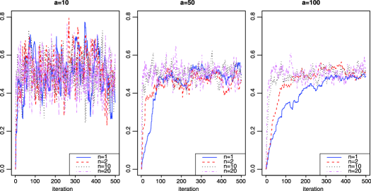
Figure 1: Traceplots of the Markov chain $\{M_{m}^{(n)},m\geq 0\}$ with $\alpha_{0}$ the Uniform distribution on $(0,1)$, $a=10,50,100$ and $n=1$ (solid blue line), $n=2$ (dashed red line), $n=10$ (dotted black line) and $n=20$ (dot-dashed violet line).

This behaviour is confirmed in the next example, where the support of the measure $\alpha$ is assumed to be unbounded.

Example 2.

Let $\alpha_{0}$ be a Gaussian distribution with parameter $(0,1)$ and let $a=10$. The behavior of ${M_{m},m\geq 0}$ has been considered in [15]. Figure 2 displays the trace plots of ${M_{m}^{(n)},m\geq 0}$ for three different initial values ($M_{0}^{(n)}=-3,0,3$), with $n=1,10,20$. Also in this case, it is clear that the convergence improves as $n$ increases. As far as the total user times are concerned, we drew similar conclusions than in Example 1.

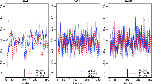
Figure 2: Traceplots of the Markov chain $\{M_{m}^{(n)},m\geq 0\}$ with $\alpha_{0}$ the Gaussian distribution with parameter $(0,1)$, $a=10$, $n=1,10,20$ and $M^{(1)}_{0}=-3$ (dashed red line), $M^{(1)}_{0}=0$ (solid blue line) and $M^{(1)}_{0}=3$ (dotted black line).

The next is an example in the mixture models context.

Example 3.

Let us consider a Gaussian kernel $k(x,\theta)$ with unknown mean $\theta$ and known variance equal to 1. If we consider the random density $f(x)=\int_{\mathbb{R}}k(x,\theta)\,\mathrm{d}P(\theta)$, where $P$ is a Dirichlet process with parameter $\alpha$, then, for any fixed $x$, $f(x)$ is a random Dirichlet mean. Therefore, if we consider the measure-valued Markov chain $\{P_{m}^{(n)},m\geq 0\}$ defined recursively as in (12), we define a sequence of random densities $\{f_{m}^{(n)}(x),m\geq 0\}$, where $f_{m}^{(n)}(x):=\int_{\mathbb{R}}k(x,\theta)\,\mathrm{d}P_{m}^{(n)}(\theta)=\theta_{m}\sum_{1}^{n}q_{m,i}^{(n)}k(x,Y_{m,i})+(1-\theta_{m})f_{m-1}^{(n)}(x)$. In each panel of Figure 3, we drew $f_{m}^{(n)}(x)$ for different values of $m$ when $n$ is fixed. In particular, we fixed $\alpha_{0}$ to be a Gaussian distribution with parameter $(0,1)$, and let $a=100$; in this case, since the “variance” of $P$ is small, the mean density $E[f](x)=\int_{\mathbb{R}}k(x,\theta)\alpha_{0}(\mathrm{d}\theta)$ (Gaussian with parameter $(0,2)$) will be very close to the random function $f(x)$, so that it can be considered an approximation of the “true” density $f(x)$. From the plots, it is clear that the convergence improves as $n$ increases: when $n=1$, only $f_{1000}^{(1)}(x)$ is close enough to the mean density $E[f](x)$, while, if $n=20$, $f_{100}^{(20)}(x)$, as well as the successive iterations, is a good approximation of $f(x)$.

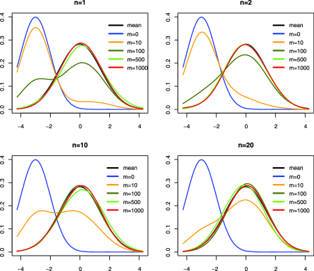
Figure 3: Plots of $f_{m}^{(n)}$ as in Example 3; $a=100$, $\alpha_{0}={\mathcal{N}}(0,1)$, $n=1,2,10,20$ and $f^{(n)}_{0}={\mathcal{N}}(\cdot;-3,1)$.

In any case, observe that even if the “true” density $f(x)$ is unknown, as when $a=1$, the improvement (as $n$ increases) is clear as well; see Figure 4, where 5 draws of $f_{m}^{(n)}(x)$, $m=1,100,1000$, are plotted for different values of $n$.

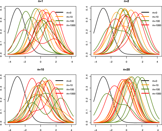
Figure 4: Plots of 5 draws from $f_{m}^{(n)}$ as in Example 3; $a=1$, $\alpha_{0}={\mathcal{N}}(0,1)$, $n=1,2,10,20$ and $f^{(n)}_{0}={\mathcal{N}}(\cdot;-3,1)$.

4 Concluding remarks and developments

The paper [12] constitutes, as far as we know, the first work highlighting the interplay between Bayesian nonparametrics on the one side and the theory of measure-valued Markov chains on the other. In the present paper, we have further studied such interplay by introducing and investigating a new measure-valued Markov chain $\{Q_{n},n\geq 1\}$ defined via exchangeable sequences of r.v.s. Two applications related to Bayesian nonparametrics have been considered: the first gives evidence that $\{Q_{n},n\geq 1\}$ is strictly related to the Newton’s algorithm of the mixture of Dirichlet process model, while the second shows how $\{Q_{n},n\geq 1\}$ can be applied in order to a define a generalization of the Feigin–Tweedie Markov chain.

An interesting development consists in investigating whether there are any new applications related to the Feigin–Tweedie Markov chain apart from the well-known application in the field of functional linear functionals of the Dirichlet process (see, e.g., [14]). The proposed generalization of the Feigin–Tweedie Markov chain represents a large class of measure-valued Markov chains $\{\{P_{m}^{(n)},m\geq 0\},n\in\mathbb{N}\}$ maintaining all the same properties of the Feigin–Tweedie Markov chain; in other terms, we have increased the flexibility of the Feigin–Tweedie Markov chain via a further parameter $n\in\mathbb{N}$. We believe that a number of different interpretations for $n$ can be investigated in order to extend the applicability of the Feigin–Tweedie Markov chain.

In this respect, an intuitive and simple extension is related to the problem of defining a (bivariate) vector of measure-valued Markov chains $\{(P_{m}^{(n_{1})},P_{m}^{(n_{2})}),m\geq 0\}$, where, for each fixed $m$, $(P_{m}^{(n_{1})},P_{m}^{(n_{2})})$ is a vector of dependent random probabilities, $n_{1}<n_{2}$ being fixed positive integers. Marginally, the two sequences $\{P_{m}^{(n_{1})},m\geq 0\}$ and $\{P_{m}^{(n_{2})},m\geq 0\}$ are defined via the recursive identity (12); the dependence is achieved using the same Pólya sequence $(Y_{m,1}^{(n_{2})},\ldots,$ $Y_{m,n_{1}}^{(n_{2})},\ldots,Y_{m,n_{2}}^{(n_{2})})$ and assuming dependence in $(\theta_{m}^{(n_{2})},\theta_{m}^{(n_{1})})$ or between $(q_{m,1}^{(n_{2})},\ldots,q_{m,n_{2}}^{(n_{2})})$ and $(q_{m,1}^{(n_{1})},\ldots,q_{m,n_{1}}^{(n_{1})})$. For instance, if, for each $m$, $Z_{m},Z_{m}^{(1)},\ldots,Z_{m}^{(n_{1})},\ldots,Z_{m}^{(n_{2})}$ are independent r.v.s, $Z_{m}$ with an Exponential distribution with parameter $a$, $Z_{m}^{(i)}$ with an Exponential distribution with parameter 1, we could define $\theta_{m}^{(n_{2})}:={{\sum_{i=1}^{n_{2}}Z_{m}^{(i)}}/{(Z_{m}+\sum_{i=1}^{n_{2}}Z_{m}^{(i)})}}$, $\theta_{m}^{(n_{1})}:={\sum_{i=1}^{n_{1}}Z_{m}^{(i)}}/(Z_{m}+\sum_{i=1}^{n_{1}}Z_{m}^{(i)})$. Of course, the dependence is related to the difference between $n_{1}$ and $n_{2}$. Work on this is ongoing.

Appendix

.1 Weak convergence for the Markov chain $\{Q_{n},n\geq 1\}$

A proof of the weak convergence of the sequence $Q_{n}=\sum_{1}^{n}q_{i}^{(n)}\delta_{Y_{i}}$ of r.p.m.s on $\mathbb{X}$ to a Dirichlet process $P$ is provided here, when the $Y_{j}$’s are a Pólya sequence with parameter measure $\alpha$. The result automatically follows from Theorem 1(ii), but this proof is interesting per se, since we use a combinatorial technique; moreover an explicit expression for the moment of order $(r_{1},\ldots,r_{k}$) of the $k$-dimensional Pólya distribution is obtained.

Let $Q_{n}$ defined in (5), where $\{Y_{j},j\geq 1\}$ are a Pólya sequence with parameter $\alpha$. Then

$$Q_{n}\Rightarrow P,$$

where $P$ is a Dirichlet process on $\mathbb{X}$ with parameter $\alpha$.

Proof.

By Theorem 4.2 in [18], it is sufficient to prove that for any measurable partition $B_{1},\ldots,B_{k}$ of $\mathbb{X}$,

$$(Q_{n}(B_{1}),\ldots,Q_{n}(B_{k}))\Rightarrow(P(B_{1}),\ldots,P(B_{k})),$$

characterizing the distribution of the limit. For any given measurable partition $B_{1},\ldots,B_{k}$ of $\mathbb{X}$, by conditioning on $Y_{1},\ldots,Y_{n}$, it can be checked that $(Q_{n}(B_{1}),\ldots,Q_{n}(B_{k-1}))$ is distributed according to a Dirichlet distribution with empirical parameter $(\sum_{1\leq i\leq n}\delta_{Y_{i}}(B_{1}),\allowbreak\ldots,\sum_{1\leq i\leq n}\delta_{Y_{i}}(B_{k-1}),\sum_{1\leq i\leq n}\delta_{Y_{i}}(B_{k}))$, and

$$\mathbb{P}(\#\{i\colon\ Y_{i}\in B_{1}\}=j_{1},\ldots,\#\{i\colon\ Y_{i}\in B_{k}\}=j_{k})$$

(18)

$$\quad={n\choose j_{1}\cdots j_{k}}\frac{(\alpha(B_{1}))_{j_{1}\uparrow 1}\cdots(\alpha(B_{k}))_{j_{k}\uparrow 1}}{(a)_{n\uparrow 1}},$$

where $(j_{1},\ldots,j_{k})\in\mathcal{D}^{(0)}_{k,n}$ with $\mathcal{D}^{(0)}_{k,n}:=\{(j_{1},\ldots,j_{k})\in\{0,\ldots,n\}^{k}:\sum_{1\leq i\leq k}j_{i}=n\}$. For any $k$-uple of nonnegative integers $(r_{1},\ldots,r_{k})$, we are going to compute the limit, for $n\rightarrow+\infty$, of the moment

$$\mathbb{E}\Biggl{[}(Q_{n}(B_{1}))^{r_{1}}\cdots(Q_{n}(B_{k-1}))^{r_{k-1}}\Biggl{(}1-\sum_{i=1}^{k-1}Q_{n}(B_{i})\Biggr{)}^{r_{k}}\Biggr{]}$$

(19)

$$\quad=\sum_{(j_{1},\ldots,j_{k})\in\mathcal{D}^{(0)}_{k,n}}{n\choose j_{1}\cdots j_{k}}\frac{(\alpha(B_{1}))_{j_{1}\uparrow 1}\cdots(\alpha(B_{k}))_{j_{k}\uparrow 1}}{(a)_{n\uparrow 1}}\frac{(j_{1})_{r_{1}\uparrow 1}\cdots(j_{k})_{r_{k}\uparrow 1}}{(n)_{(r_{1}+\cdots+r_{k})\uparrow 1}},$$

where in general $(x)_{n\uparrow\alpha}$ denotes the Pochhammer symbol for the $n$th factorial power of $x$ with increment $\alpha$, that is $(x)_{n\uparrow\alpha}:=\prod_{0\leq i\leq n-1}(x+i\alpha)$. We will show that, as $n\rightarrow+\infty$,

$$\mathbb{E}\Biggl{[}(Q_{n}(B_{1}))^{r_{1}}\cdots(Q_{n}(B_{k-1}))^{r_{k-1}}\Biggl{(}1-\sum_{i=1}^{k-1}Q_{n}(B_{i})\Biggr{)}^{r_{k}}\Biggr{]}$$

$$\quad\rightarrow\mathbb{E}\Biggl{[}(P(B_{1})\big{)}^{r_{1}}\cdots(P(B_{k-1}))^{r_{k-1}}\Biggl{(}1-\sum_{i=1}^{k-1}P(B_{i})\Biggr{)}^{r_{k}}\Biggr{]},$$

where $P$ is a Dirichlet process on $\mathbb{X}$ with parameter measure $\alpha$, that is, the r.v. $(P(B_{1}),\ldots,P(B_{k-1}))$ has Dirichlet distribution with parameter $(\alpha(B_{1}),\ldots,\alpha(B_{k-1}),\allowbreak\alpha(B_{k}))$. This will be sufficient to characterize the distribution of the limit $Q^{*}$, because of the boundedness of the support of the limit distribution. First of all, we prove the convergence for $k=2$, which corresponds to the one-dimensional case. In particular, we have

$$\mathbb{E}\bigl{[}(Q_{n}(B_{1}))^{r_{1}}\bigl{(}1-(Q_{n}(B_{1}))\bigr{)}^{r_{2}}\bigr{]}$$

$$\quad=\frac{1}{(n)_{(r_{1}+r_{2})\uparrow 1}}\sum_{(j_{1},j_{2})\in\mathcal{D}^{(0)}_{2,n}}{n\choose j_{1},j_{2}}\frac{(\alpha(B_{1}))_{j_{1}\uparrow 1}(\alpha(B_{2}))_{j_{2}\uparrow 1}}{(a)_{n\uparrow 1}}(j_{1})_{r_{1}\uparrow 1}(j_{2})_{r_{2}\uparrow 1}$$

$$\quad=\frac{1}{(n)_{(r_{1}+r_{2})\uparrow 1}}\sum_{t_{1}=1}^{r_{1}}|s(r_{1},t_{1})|\sum_{s_{1}=1}^{t_{1}}S(t_{1},s_{1})\sum_{t_{2}=1}^{r_{2}}|s(r_{2},t_{2})|\sum_{s_{2}=1}^{t_{2}}S(t_{2},s_{2})$$

$$\qquad{}\times\sum_{(j_{1},j_{2})\in\mathcal{D}^{(0)}_{2,n}}{n\choose j_{1},j_{2}}\frac{(\alpha(B_{1}))_{j_{1}\uparrow 1}(\alpha(B_{2}))_{j_{2}\uparrow 1}}{(a)_{n\uparrow 1}}(j_{1})_{s_{1}\downarrow 1}(j_{2})_{s_{2}\downarrow 1},$$

where $(x)_{n\downarrow 1}:=(-1)^{-n}(-x)_{n\uparrow 1}$ and $s(\cdot,\cdot)$ and $S(\cdot,\cdot)$ are the Stirling number of the first and second kind, respectively. Let us consider the following numbers, where $s_{1}$, $s_{2}$ are nonnegative integers and $n=1,2,\ldots,$

$$C_{n}^{(s_{1},s_{2})}:=\sum_{(j_{1},j_{2})\in\mathcal{D}^{(0)}_{2,n}}{n\choose j_{1},j_{2}}\frac{(\alpha(B_{1}))_{j_{1}\uparrow 1}(\alpha(B_{2}))_{j_{2}\uparrow 1}}{(a)_{n\uparrow 1}}(j_{1})_{s_{1}\downarrow 1}(j_{2})_{s_{2}\downarrow 1},$$

and prove they satisfy a recursive relation. In particular,

$$C_{n+1}^{(s_{1},s_{2})} = \sum_{(j_{1},j_{2})\in\mathcal{D}^{(0)}_{2,n+1}}{n+1\choose j_{1},j_{2}}\frac{(\alpha(B_{1}))_{j_{1}\uparrow 1}(\alpha(B_{2}))_{j_{2}\uparrow 1}}{(a)_{(n+1)\uparrow 1}}(j_{1})_{s_{1}\downarrow 1}(j_{2})_{s_{2}\downarrow 1}$$

$$= \sum_{j_{1}=0}^{n}{n+1\choose j_{1}+1}\frac{(\alpha(B_{1}))_{(j_{1}+1)\uparrow 1}(\alpha(B_{2}))_{(n-j_{1})\uparrow 1}}{(a)_{(n+1)\uparrow 1}}(j_{1}+1)_{s_{1}\downarrow 1}(n-j_{1})_{s_{2}\downarrow 1}$$

$$= \frac{(n+1)(\alpha(B_{1})+s_{1}-1)}{(a+n)}C_{n}^{(s_{1}-1,s_{2})}+\frac{n+1}{(a+n)}C_{n}^{(s_{1},s_{2})},$$

so that the following recursive equation holds

$$C_{n+1}^{(s_{1},s_{2})}=\frac{(n+1)(\alpha(B_{1})+s_{1}-1)}{(a+n)}C_{n}^{(s_{1}-1,s_{2})}+\frac{n+1}{(a+n)}C_{n}^{(s_{1},s_{2})}.$$ (20)

Therefore, starting from $C_{n}^{(0,0)}=1$, $C_{n}^{(0,1)}={n\alpha(B_{2})/a}$, we have

$$C_{n}^{(1,1)} = \sum_{i=0}^{n-1}\frac{(i+1)\alpha(B_{1})}{(a+i)}C_{i}^{(0,1)}\prod_{j=i+1}^{n-1}\frac{j+1}{a+j}$$

$$= \frac{\Gamma(n+1)\alpha(B_{1})}{\Gamma(a+n)}\sum_{i=0}^{n-1}\frac{\Gamma(a+i)}{\Gamma(i+1)}C_{i}^{(0,1)}$$

$$= \frac{\Gamma(n+1)\alpha(B_{1})}{\Gamma(a+n)}\sum_{i=0}^{n-1}\frac{\Gamma(a+i)}{\Gamma(i+1)}\frac{i\alpha(B_{2})}{a}=\frac{\alpha(B_{1})\alpha(B_{2})(n)_{2\downarrow 1}}{(a)_{2\uparrow 1}},$$

and by (20) we obtain $C_{n}^{(s_{1},s_{2})}=(\alpha(B_{1}))_{s_{1}\uparrow 1}(\alpha(B_{2}))_{s_{2}\uparrow 1}(n)_{(s_{1}+s_{2})\downarrow 1}/(a)_{(s_{1}+s_{2})\uparrow 1}$. Thus,

$$\lim_{n\rightarrow+\infty}\mathbb{E}\bigl{[}(H_{n}(B_{1}))^{r_{1}}\bigl{(}1-(H_{n}(B_{1}))\bigr{)}^{r_{2}}\bigr{]}$$

$$\quad=\sum_{t_{1}=0}^{r_{1}}|s(r_{1},t_{1})|\sum_{s_{1}=0}^{t_{1}}S(t_{1},s_{1})\sum_{t_{2}=0}^{r_{2}}|s(r_{2},t_{2})|\sum_{s_{2}=0}^{t_{2}}S(t_{2},s_{2})\lim_{n\rightarrow+\infty}\frac{C_{n}^{(s_{1},s_{2})}}{(n)_{(r_{1}+r_{2})\uparrow 1}}$$

$$\quad=|s(r_{1},r_{1})|S(r_{1},r_{1})|s(r_{2},r_{2})|S(r_{2},r_{2})\frac{(\alpha(B_{1}))_{r_{1}\uparrow 1}(\alpha(B_{2}))_{r_{2}\uparrow 1}}{(a)_{(r_{1}+r_{2})\uparrow 1}}$$

$$\quad=\frac{(\alpha(B_{1}))_{r_{1}\uparrow 1}(\alpha(B_{2}))_{r_{2}\uparrow 1}}{(a)_{(r_{1}+r_{2})\uparrow 1}}.$$

The last expression is exactly $\mathbb{E}[(P(B_{1}))^{r_{1}}(1-P(B_{1}))^{r_{2}}]$, where $P(B_{1})$ has Beta distribution with parameter $(\alpha(B_{1}),\alpha(B_{2}))$.

This proof can be easily generalized to the case $k>2$. Analogously to the one-dimensional case, we can write

$$\mathbb{E}\Biggl{[}(Q_{n}(B_{1}))^{r_{1}}\cdots(Q_{n}(B_{k-1}))^{r_{k-1}}\Biggl{(}1-\sum_{i=1}^{k-1}Q_{n}(B_{i})\Biggr{)}^{r_{k}}\Biggr{]}$$

$$\quad=\frac{1}{(n)_{(r_{1}+\cdots+r_{k})\uparrow 1}}\sum_{(j_{1},\ldots,j_{k})\in\mathcal{D}^{(0)}_{k,n}}{n\choose j_{1}\cdots j_{k}}\frac{(\alpha(B_{1}))_{j_{1}\uparrow 1}\cdots(\alpha(B_{k}))_{j_{k}\uparrow 1}}{(a)_{n\uparrow 1}}(j_{1})_{r_{1}\uparrow 1}\cdots(j_{k})_{r_{k}\uparrow 1}$$

$$\quad=\frac{1}{(n)_{(r_{1}+\cdots+r_{k})\uparrow 1}}\sum_{t_{1}=0}^{r_{1}}|s(r_{1},t_{1})|\sum_{s_{1}=0}^{t_{1}}S(t_{1},s_{1})\cdots\sum_{t_{k}=0}^{r_{k}}|s(r_{k},t_{k})|\sum_{s_{k}=0}^{t_{k}}S(t_{k},s_{k})$$

$$\qquad{}\times\sum_{(j_{1},\ldots,j_{k})\in\mathcal{D}^{(0)}_{k,n}}{n\choose j_{1}\cdots j_{k}}\frac{(\alpha(B_{1}))_{j_{1}\uparrow 1}\cdots(\alpha(B_{k}))_{j_{k}\uparrow 1}}{(a)_{n\uparrow 1}}(j_{1})_{s_{1}\downarrow 1}\cdots(j_{k})_{s_{k}\downarrow 1}$$

and, as before, define

$$C_{n}^{(s_{1},\ldots,s_{k})}:=\sum_{(j_{1},\ldots,j_{k})\in\mathcal{D}^{(0)}_{k,n}}{n\choose j_{1}\cdots j_{k}}\frac{(\alpha(B_{1}))_{j_{1}\uparrow 1}\cdots(\alpha(B_{k}))_{j_{k}\uparrow 1}}{(a)_{n\uparrow 1}}\times(j_{1})_{s_{1}\downarrow 1}\cdots(j_{k})_{s_{k}\downarrow 1}$$

and prove they satisfy a recursive relation. Observe that $C_{n}^{(s_{1},\ldots,s_{k})}/{(n)_{(r_{1}+\cdots+r_{k})\uparrow 1}}$ is the moment of order $(r_{1},\ldots,r_{k})$ of the $k$-dimensional Pólya distribution by definition. Therefore, for $k>2$

$$C_{n}^{(s_{1},\ldots,s_{k})} = \sum_{j_{k}=0}^{n}{n\choose j_{k}}\frac{(\alpha(B_{k}))_{j_{k}\uparrow 1}(a-\alpha(B_{k}))_{(n-j_{k})\uparrow 1}(j_{k})_{s_{k}\downarrow 1}}{(a)_{n\uparrow 1}}$$

$$\hphantom{\sum_{j_{k}=0}^{n}}{}\times\sum_{(j_{1},\ldots,j_{k-1})\in\mathcal{D}^{(0)}_{k-1,n-j_{k}}}{n-j_{k}\choose j_{1}\cdots j_{k-1}}\frac{(\alpha(B_{1}))_{j_{1}\uparrow 1}\cdots(\alpha(B_{k-1}))_{j_{k-1}\uparrow 1}}{(a-\alpha(B_{k}))_{(n-j_{k})\uparrow 1}}$$

$$\hskip 10.0pt\hphantom{\sum_{j_{k}=0}^{n}\sum_{(j_{1},\ldots,j_{k-1})\in\mathcal{D}^{(0)}_{k-1,n-j_{k}}}}{}\times(j_{1})_{s_{1}\downarrow 1}\cdots(j_{k-1})_{s_{k-1}\downarrow 1}$$

$$= \sum_{j_{k}=0}^{n}{n\choose j_{k}}\frac{(\alpha(B_{k}))_{j_{k}\uparrow 1}(a-\alpha(B_{k}))_{(n-j_{k})\uparrow 1}(j_{k})_{s_{k}\downarrow 1}}{(a)_{n\uparrow 1}}$$

$$\hphantom{\sum_{j_{k}=0}^{n}}{}\times\frac{(\alpha(B_{1}))_{s_{1}\uparrow 1}\cdots(\alpha(B_{k-1}))_{s_{k-1}\uparrow 1}(n-j_{k})_{(s_{1}+\cdots+s_{k-1})\downarrow 1}}{(a-\alpha(B_{k}))_{(s_{1}+\cdots+s_{k-1})\uparrow 1}},$$

where the last equality follows by induction hypothesis (we already proved the base case $k=2$ in (20)). Then, following the same steps of the one-dimensional case, we can recover a recursive equation for $C_{n}^{(s_{1},\ldots,s_{k})}$,

$$C_{n+1}^{(s_{1},\ldots,s_{k})}=\frac{(n+1)(\alpha(B_{k})+s_{k}-1)}{a+n}C_{n}^{(s_{1},\ldots,s_{k-1},s_{k}-1)}+\frac{n+1}{a+n}C_{n}^{(s_{1},\ldots,s_{k})}.$$ (21)

Starting from $C_{n}^{(0,\ldots,0)}=1$, $C_{n}^{(0,\ldots,0,1,0,\ldots,0)}={n\alpha(B_{j})/a}$ and

$$C_{n}^{(1,\ldots,1)} = \sum_{i=0}^{n-1}\frac{(i+1)\alpha(B_{k})}{(a+i)}C_{i}^{(1,\ldots,1,0)}\prod_{j=i+1}^{n-1}\frac{j+1}{a+j}$$

$$= \frac{\Gamma(n+1)}{\Gamma(a+n)}\frac{(\alpha(B_{1}))_{s_{1}\uparrow 1}\cdots(\alpha(B_{k-1}))_{s_{p-1}\uparrow 1}\alpha(B_{k})}{(a-\alpha(B_{k}))_{(s_{1}+\cdots+s_{k-1})\uparrow 1}}\sum_{i=0}^{n-1}\frac{\Gamma(a+i)}{\Gamma(1+i)}C_{i}^{(1,\ldots,1,0)}$$

$$= \frac{\Gamma(n+1)}{\Gamma(a+n)}\frac{(\alpha(B_{1}))_{s_{1}\uparrow 1}\cdots(\alpha(B_{k-1}))_{s_{k-1}\uparrow 1}\alpha(B_{k})}{(a-\alpha(B_{k}))_{(s_{1}+\cdots+s_{k-1})\uparrow 1}}$$

$${}\times(-1)^{k+1}\sum_{i=0}^{n-1}\frac{\Gamma(a+i)}{\Gamma(1+i)}\frac{(a-\alpha(B_{k}))_{i\uparrow 1}(-i)_{(k-1)\uparrow 1}}{(a)_{i\uparrow 1}}$$

$$\hphantom{{}\times(-1)^{k+1}\sum_{i=0}^{n-1}}{}\times\frac{\Gamma(-a+\alpha(B_{k})-i+1)\Gamma(-k-a+2)}{\Gamma(-a-i+1)\Gamma(-a+\alpha(B_{k})+2-k)}$$

$$= \frac{\alpha(B_{1})\cdots\alpha(B_{k})(n)_{k\downarrow 1}}{(a)_{(k\uparrow 1)}},$$

by repeated application of (21), we obtain

$$C_{n}^{(s_{1},\ldots,s_{k})}=\frac{(\alpha(B_{1}))_{s_{1}\uparrow 1}\cdots(\alpha(B_{k}))_{s_{k}\uparrow 1}(n)_{(s_{1}+\cdots+s_{k})\downarrow 1}}{(a)_{(s_{1}+\cdots+s_{k})\uparrow 1}}.$$

Thus,

$$\lim_{n\rightarrow+\infty}\mathbb{E}\Biggl{[}(Q_{n}(B_{1}))^{r_{1}}\cdots(Q_{n}(B_{k-1}))^{r_{k-1}}\Biggl{(}1-\sum_{i=1}^{k-1}Q_{n}(B_{i})\Biggr{)}^{r_{p}}\Biggr{]}$$

$$\quad=\sum_{t_{1}=0}^{r_{1}}|s(r_{1},t_{1})|\sum_{s_{1}=0}^{t_{1}}S(t_{1},s_{1})\cdots\sum_{t_{k}=0}^{r_{k}}|s(r_{k},t_{k})|\sum_{s_{k}=0}^{t_{k}}S(t_{k},s_{k})\lim_{n\rightarrow+\infty}\frac{C_{n}^{(s_{1},\ldots,s_{k})}}{(n)_{(r_{1}+\cdots+r_{k})\uparrow 1}}$$

$$\quad=|s(r_{1},r_{1})|S(r_{1},r_{1})\cdots|s(r_{k},r_{k})|S(r_{k},r_{k})\frac{(\alpha(B_{1}))_{r_{1}\uparrow 1}\cdots(\alpha(B_{k}))_{r_{k}\uparrow 1}}{(a)_{(r_{1}+\cdots+r_{k})\uparrow 1}}$$

$$\quad=\frac{(\alpha(B_{1}))_{r_{1}\uparrow 1}\cdots(\alpha(B_{k}))_{r_{k}\uparrow 1}}{(a)_{(r_{1}+\cdots+r_{k})\uparrow 1}}$$

$$\quad=\mathbb{E}\Biggl{[}(P(B_{1}))^{r_{1}}\cdots(P(B_{k-1}))^{r_{k-1}}\Biggl{(}1-\sum_{i=1}^{k-1}P(B_{i})\Biggr{)}^{r_{k}}\Biggr{]},$$

where $P$ is a Dirichlet process with parameter $\alpha$. ∎

.2 Solution of the distributional equation

Here, we provide an alternative proof for the solution of the distributional equation (3) introduced by [11].

For any fixed integer $n\geq 1$, the distributional equation

$$P^{(n)}\stackrel{{\scriptstyle\mathrm{d}}}{{=}}\theta\sum_{i=1}^{n}q_{i}^{(n)}\delta_{Y_{i}}+(1-\theta)P^{(n)}$$

has the Dirichlet process with parameter $\alpha$ as its unique solution, assuming the independence between $P^{(n)}$, $\theta,(q_{1}^{(n)},\ldots,q_{n}^{(n)})$ and $(Y_{1},\ldots,Y_{n})$ in the right-hand side.

Proof.

From Skorohod’s theorem, it follows that there exist $n$ independent r.v.s $\xi_{1},\ldots,\xi_{n}$ such that $\xi_{i}$ has Beta distribution with parameter $(1,n-i)$ for $i=1,\ldots,n$ and $q_{1}^{(n)}=\xi_{1}$ and $q_{i}^{(n)}=\xi_{i}\prod_{1\leq j\leq i-1}(1-\xi_{j})$ for $i=2,\ldots,n$; in particular, by a simple transformation of r.v.s, it follows that $(q_{1}^{(n)},\ldots,q_{n}^{(n)})$ is distributed according to a Dirichlet distribution function with parameter $(1,\ldots,1)$. Further, since $\xi_{n}=1$ a.s., then $\sum_{1\leq i\leq n}q_{i}^{(n)}=1$ a.s. and it can be verified by induction that

$$1-\sum_{i=1}^{j}q_{i}^{(n)}=\prod_{i=1}^{j}(1-\xi_{i}),\qquad j=1,\ldots,n-1.$$

Let $B_{1},\ldots,B_{k}$ be a measurable partition of $\mathbb{X}$. We first prove that conditionally on $Y_{1},\ldots,Y_{n}$, the finite dimensional distribution of the r.p.m. $\sum_{1\leq i\leq n}q_{i}^{(n)}\delta_{Y_{i}}$ is the Dirichlet distribution with the empirical parameter $(\sum_{1\leq i\leq n}\delta_{Y_{i}}(B_{1}),\ldots,\sum_{1\leq i\leq n}\delta_{Y_{i}}(B_{k}))$. Actually, since

$$\Biggl{(}\Biggl{(}\sum_{i=1}^{n}q_{i}^{(n)}\delta_{Y_{i}}\Biggr{)}(\cdot,B_{1}),\ldots,\Biggl{(}\sum_{i=1}^{n}q_{i}^{(n)}\delta_{Y_{i}}\Biggr{)}(\cdot,B_{k})\Biggr{)}$$

$$\quad=\Biggl{(}\sum_{i=1}^{n}q_{i}^{(n)}\delta_{Y_{i}}(B_{1}),\ldots,\sum_{i=1}^{n}q_{i}^{(n)}\delta_{Y_{i}}(B_{k})\Biggr{)}$$

$$\quad=\Biggl{(}\sum_{i:Y_{i}\in B_{1}}q_{i}^{(n)},\ldots,\sum_{i:Y_{i}\in B_{k}}q_{i}^{(n)}\Biggr{)},$$

then, conditionally on the r.v.s $Y_{1},\ldots,Y_{n}$, the r.v. $(\sum_{i:Y_{i}\in B_{1}}q_{i}^{(n)}$, $\ldots,$$\sum_{i:Y_{i}\in B_{k}}q_{i}^{(n)})$ is distributed according to a Dirichlet distribution with parameter $(n_{1},\ldots,$ $n_{k})$, where $n_{i}=\sum_{1\leq j\leq n}\delta_{Y_{j}}(B_{i})$ for $i=1,\ldots,k$. Conditionally on $Y_{1},\ldots,Y_{n}$, the finite dimensional distributions of the right-hand side of (3) are Dirichlet with updated parameter $((\alpha(B_{1})+\sum_{1\leq i\leq n}\delta_{Y_{i}}(B_{1}),\ldots,\alpha(B_{k})+\sum_{1\leq i\leq n}\delta_{Y_{i}}(B_{k}))$. This argument verifies that the Dirichlet process with parameter $\alpha$ satisfies the distributional equation (3). This solution is unique by Lemma 3.3 in [33] (see also [37], Section 1). ∎

.3 Proofs of the theorems in Section 3

Proof of Theorem 3 The proof is based on the “standard” result that properties (e.g., weak convergence) of sequences of r.p.m.s can be proved via analogous properties of the sequences of their linear functionals.

First of all, we prove that if $g\mathchoice{\nobreak\,\colon}{\nobreak\,\colon}{\nobreak\,\colon\;}{\nobreak\,\colon\;}\mathbb{X}\mapsto\mathbb{R}$ is a bounded and continuous function, then $\{G^{(n)}_{m},m\geq 0\}$ with $G_{m}^{(n)}:=\int_{\mathbb{X}}g(x)P^{(n)}_{m}(\mathrm{d}x)$ is a Markov chain on $\mathbb{R}$ with unique invariant measure $\Pi_{g}$. From (12), it follows that $\{G^{(n)}_{m},m\geq 1\}$ is a Markov chain on $\mathbb{R}$ restricted to the compact set $[-\sup_{\mathbb{X}}|g(x)|,\sup_{\mathbb{X}}|g(x)|]$ and it has at least one finite invariant measure if it is a weak Feller Markov chain. In fact, for a fixed $y\in\mathbb{R}$

$$\operatorname{lim\,inf}\limits_{x\rightarrow x^{\ast}}\mathbb{P}\bigl{(}G^{(n)}_{m}\leq y\big{|}G^{(n)}_{m-1}=x\bigr{)}$$

$$\quad=\operatorname{lim\,inf}\limits_{x\rightarrow x^{\ast}}\mathbb{P}\Biggl{(}\theta_{m}\sum_{i=1}^{n}q_{m,i}^{(n)}g(Y_{m,i})\leq y-x(1-\theta_{m})\Biggr{)}$$

$$\quad\geq\int_{(0,1)}\liminf_{x\rightarrow x^{\ast}}\mathbb{P}\Biggl{(}\sum_{i=1}^{n}q_{m,i}^{(n)}g(Y_{m,i})\leq\frac{y-x(1-z)}{z}\Biggr{)}\mathbb{P}(\theta_{m}\in\mathrm{d}z)$$

$$\quad=\int_{(0,1)}\mathbb{P}\Biggl{(}\sum_{i=1}^{n}q_{m,i}^{(n)}g(Y_{m,i})\leq\frac{y-x^{\ast}(1-z)}{z}\Biggr{)}\mathbb{P}(\theta_{m}\in\mathrm{d}z)$$

$$\quad=\mathbb{P}\bigl{(}G^{(n)}_{m}\leq y\big{|}G^{(n)}_{m-1}=x^{\ast}\bigr{)},$$

since the distribution of $\sum_{1\leq i\leq n}q_{m,i}^{(n)}g(Y_{m,i})$ has at most a countable numbers of atoms and $\theta_{m}$ is absolutely continuous. From Proposition 4.3 in [36], if we show that $\{G^{(n)}_{m},\break m\geq 0\}$ is $\phi$-irreducible for a finite measure $\phi$, then the Markov chain is positive recurrent and the invariant measure $\Pi_{g}$ is unique. Let us consider the following event $E:=\{Y_{1,1}=Y_{1,2}=\cdots=Y_{1,n}\}$. Then for a finite measure $\phi$ we have to prove that if $\phi(A)>0$, then $\mathbb{P}(G^{(n)}_{1}\in A|G^{(n)}_{0})>0$ for any $G^{(n)}_{0}$. We observe that

$$\mathbb{P}\bigl{(}G^{(n)}_{1}\in A\big{|}G^{(n)}_{0}\bigr{)} = \mathbb{P}\bigl{(}G^{(n)}_{1}\in A\big{|}G^{(n)}_{0},E\bigr{)}\mathbb{P}\bigl{(}E|G^{(n)}_{0}\bigr{)}+\mathbb{P}\bigl{(}G^{(n)}_{1}\in A\big{|}G^{(n)}_{0},E^{c}\bigr{)}\mathbb{P}\bigl{(}E^{c}|G^{(n)}_{0}\bigr{)}$$

$$\geq \mathbb{P}\bigl{(}G^{(n)}_{1}\in A\big{|}G^{(n)}_{0},E\bigr{)}\mathbb{P}(E).$$

Therefore, since $\mathbb{P}(E)>0$, using the same argument in Lemma 2 in [12], we conclude that $\mathbb{P}(G^{(n)}_{1}\in A|G^{(n)}_{0},E)>0$ for a suitable measure $\phi$ such that $\phi(A)>0$. Finally, we prove the aperiodicity of $\{G_{m}^{(n)},m\geq 0\}$ by contradiction. If the chain is periodic with period $d>1$, the exist $d$ disjoint sets $D_{1},\ldots,D_{d}$ such that $\mathbb{P}(G^{(n)}_{m}\in D_{i+1}|G^{(n)}_{m-1}=x)=1$ for all $x\in D_{i}$ and for $i=1,\ldots,d-1$. This implies $\mathbb{P}(z\sum_{i=1}^{n}q_{m,i}^{(n)}g(Y_{m,i})+(1-z)x\in D_{i+1})=1$ for almost every $z$ with respect to the Lebesgue measure restricted to $(0,1)$. Thus, $\mathbb{P}(\sum_{i=1}^{n}q_{m,i}^{(n)}g(Y_{m,i})\in D_{i+1})=1$ for $i=0,\ldots,d-1$. For generic $\alpha$ and $g$, this is in contradiction with the assumption $d>1$. By Theorem 13.3.4(ii) in [22], $G_{m}^{(n)}$ converges in distribution for $\Pi_{g}$-almost all starting points $G_{0}^{(n)}$. In particular, $\{G^{(n)}_{m},m\geq 0\}$ converges weakly for $\Pi_{g}$-almost all starting points $G^{(n)}_{0}$.

From the arguments above, it follows that, for all $g$ bounded and continuous, there exists a r.v. $G$ such that $G^{(n)}_{m}\Rightarrow G$ as $m\rightarrow+\infty$ for $\Pi_{g}$-almost all starting points $G^{(n)}_{0}$. Therefore, for Lemma 5.1 in [18] there exists a r.p.m. $P$ such that $P^{(n)}_{m}\Rightarrow P$ as $m\rightarrow+\infty$ and $G\stackrel{{\scriptstyle\mathrm{d}}}{{=}}\int_{\mathbb{X}}g(x)P(\cdot,\mathrm{d}x)$ for all $g\in C(\mathbb{R})$. This implies that the law of $P$ is an invariant measure for the Markov chain $\{P^{(n)}_{m},m\geq 0\}$. Then, as $m\rightarrow+\infty$,

$$\int_{\mathbb{X}}g(x)\,\mathrm{d}P^{(n)}_{m}(\cdot,\mathrm{d}x)\Rightarrow\int_{\mathbb{X}}g(x)P(\cdot,\mathrm{d}x)$$

and the limit is unique for any $g\in C(\mathbb{R})$. Since for any random measure $\zeta_{1}$ and $\zeta_{2}$ we know that $\zeta_{1}\stackrel{{\scriptstyle\mathrm{d}}}{{=}}\zeta_{2}$ if and only if $\int_{\mathbb{X}}g(x)\zeta_{1}(\cdot,\mathrm{d}x)=\int_{\mathbb{X}}g(x)\zeta_{2}(\cdot,\mathrm{d}x)$ for any $g\in C(\mathbb{R})$ (see Theorem 3.1. in [18]), the invariant measure for the Markov chain $\{P^{(n)}_{m},m\geq 0\}$ is unique. By the definition of $\{P^{(n)}_{m},m\geq 0\}$, it is straightforward to show that the limit $P$ must satisfy (3) so that $P$ is the Dirichlet process with parameter $\alpha$.

Proof of Theorem 4 The proof is a straightforward adaptation of the proof of Theorem 2 in [12], using

$$f(G^{(n)}_{1}) = \log\Biggl{(}1+\Biggl{|}\theta_{1}\sum_{i=1}^{n}q_{1,i}^{(n)}g(Y_{1,i})+(1-\theta_{1})G^{(n)}_{0}\Biggr{|}\Biggr{)}$$

$$\leq \sum_{i=1}^{n}\log\bigl{(}1+|g(Y_{1,i})|\bigr{)}+\log\bigl{(}1+(1-\theta_{1})\big{|}G^{(n)}_{0}|\bigr{)}$$

instead of their inequality (8).

Proof of Theorem 5 As regards (i), given the definition of stochastically monotone Markov chain, we have that for $z_{1}<z_{2}$, $s\in\mathbb{R}$,

$$p^{(n)}_{1}(z_{1},(-\infty,s)) = \mathbb{P}\Biggl{(}\theta_{1}\sum_{i=1}^{n}q_{1,i}^{(n)}Y_{1,i}+(1-\theta_{1})z_{1}<s\Biggr{)}$$

$$\geq \mathbb{P}\Biggl{(}\theta_{1}\sum_{i=1}^{n}q_{1,i}^{(n)}Y_{1,i}+(1-\theta_{1})z_{2}<a\Biggr{)}$$

$$= p^{(n)}_{1}(z_{2},(-\infty,s)).$$

As far as (ii) is concerned, we first prove that, under condition (15), the Markov chain $\{M^{(n)}_{m},m\geq 0\}$ satisfies the Foster–Lyapunov condition for the function $V(x)=1+|x|$. This property implies the geometric ergodicity of the $\{M^{(n)}_{m},m\geq 0\}$ (see [22], Chapter 15). We have

$$pV(x) = \int_{\mathbb{X}}(1+|y|)p(x,\mathrm{d}y)=1+\mathbb{E}\Biggl{[}\Biggl{|}\theta_{1}\sum_{i=1}^{n}q_{1,i}^{(n)}Y_{1,i}+(1-\theta_{1})x\Biggr{|}\Biggr{]}$$

$$\leq 1+\mathbb{E}[\theta_{1}]\sum_{i=1}^{n}E\bigl{[}\bigl{|}q_{1,i}^{(n)}Y_{1,i}\bigr{|}\bigr{]}+|x|\mathbb{E}[1-\theta_{1}]$$

$$\leq 1+\frac{n}{n+a}\sum_{i=1}^{n}\mathbb{E}\bigl{[}\bigl{|}q_{1,i}^{(n)}Y_{1,i}\bigr{|}\bigr{]}+\frac{a}{n+a}|x|=1+\frac{n}{n+a}\mathbb{E}[|Y_{1,1}|]+\frac{a}{n+a}|x|.$$

Therefore, we are looking for the small set $C^{(n)}$ such that the Foster–Lyapunov condition holds, that is, a small set $C^{(n)}$ such that

$$1+\frac{n}{n+a}\mathbb{E}[|Y_{1,1}|]+\frac{a}{n+a}|x|\leq\lambda(1+|x|)+b\mathbbl{1}_{C^{(n)}}(x)$$ (22)

for some constant $b<+\infty$ and $0<\lambda<1$. If $C^{(n)}=[-K^{(n)}(\lambda),K^{(n)}(\lambda)]$, where

$$K^{(n)}(\lambda):=\frac{1-\lambda+n/(n+a)\mathbb{E}[|Y_{1,1}|]}{\lambda-a/(n+a)},$$

then, condition (22) holds for all

$$\lambda\in\biggl{(}\frac{a}{n+a},1\biggr{)},\qquad b\geq 1-\lambda+\frac{n}{n+a}\mathbb{E}[|Y_{1,1}|].$$

As in the proof of Theorem 3, we can prove that the Markov chain $\{M^{(n)}_{m},m\geq 0\}$ is weak Feller; then, since $C^{(n)}$ is a compact set, it is a small set (see [35]). As regards (iii), the proof follows by standard arguments. See, for instance, the proof of Theorem 1 in [15].

Proof of Remark 1 As we have already mentioned, the geometric ergodicity follows if a Foster–Lyapunov condition holds. Let $V(x)=1+|x|^{s}$; then, if $\mathbb{E}[(1+|\sum_{1\leq i\leq n}q_{1,i}^{(n)}Y_{1,i}|)^{s}]<+\infty$, it is straightforward to prove that the Foster–Lyapunov condition $PV(x)\leq\lambda V(x)+b\mathbbl{1}_{\tilde{C}^{(n)}}(x)$ holds for some constant $b<+\infty$, and $\lambda$ such that

$$\mathbb{E}[(1-\theta_{1})^{s}]=\frac{\Gamma(a+s)\Gamma(a+n)}{\Gamma(a)\Gamma(a+s+n)}<\lambda<1$$

and for some compact set $\tilde{C}^{(n)}$. Of course (16) implies $\mathbb{E}[(1+|\sum_{1\leq i\leq n}q_{1,i}^{(n)}Y_{1,i}|)^{s}]<+\infty;$ in fact, conditioning on the random number $N$ of distinct values $Y_{1,1}^{\ast},\ldots,Y_{1,N}^{\ast}$ in $Y_{1,1},\ldots,Y_{1,n}$, $1\leq N\leq n$, we have

$$\Biggl{|}\sum_{i=1}^{n}q_{1,i}^{(n)}Y_{1,i}\Biggr{|}\leq\sum_{i=1}^{N}\tilde{q}_{1,i}^{(n)}|Y^{\ast}_{1,i}|\leq\max\{|Y_{1,1}^{\ast}|,\ldots,|Y_{1,N}^{\ast}|\}.$$

Since $\{Y_{1,1}^{\ast},\ldots,Y_{1,N}^{\ast}\}$ are independent and identically distributed according to $\alpha_{0}$, then

$$\mathbb{E}\Biggl{[}\Biggl{|}\sum_{i=1}^{n}q_{1,i}^{(n)}Y_{1,i}\Biggr{|}^{s}\Biggr{]}\leq\int_{0}^{+\infty}y^{s}N(A_{0}(y))^{N-1}\alpha_{0}(\mathrm{d}y)\leq N\int_{0}^{+\infty}y^{s}\alpha_{0}(\mathrm{d}y)\leq n\mathbb{E}[|Y_{1,i}|^{s}]<+\infty,$$

where $A_{0}$ is the distribution corresponding to the probability measure $\alpha_{0}$, and this is equivalent to $\mathbb{E}[(1+|\sum_{1\leq i\leq n}q_{1,i}^{(n)}Y_{1,i}|)^{s}]<+\infty$.

References

- [1] {barticle}[mr] \bauthor\bsnmBerti, \bfnmPatrizia\binitsP., \bauthor\bsnmPratelli, \bfnmLuca\binitsL. &\bauthor\bsnmRigo, \bfnmPietro\binitsP. (\byear2006). \btitleAlmost sure weak convergence of random probability measures. \bjournalStochastics \bvolume78 \bpages91–97. \biddoi=10.1080/17442500600745359, issn=1744-2508, mr=2236634 \endbibitem
- [2] {barticle}[mr] \bauthor\bsnmBlackwell, \bfnmDavid\binitsD. &\bauthor\bsnmMacQueen, \bfnmJames B.\binitsJ.B. (\byear1973). \btitleFerguson distributions via Pólya urn schemes. \bjournalAnn. Statist. \bvolume1 \bpages353–355. \bidissn=0090-5364, mr=0362614 \endbibitem
- [3] {bbook}[mr] \bauthor\bsnmChow, \bfnmYuan Shih\binitsY.S. &\bauthor\bsnmTeicher, \bfnmHenry\binitsH. (\byear1997). \btitleProbability Theory: Independence, Interchangeability, Martingales, \bedition3rd ed. \bseriesSpringer Texts in Statistics. \baddressNew York: \bpublisherSpringer. \bidmr=1476912 \endbibitem
- [4] {barticle}[mr] \bauthor\bsnmCifarelli, \bfnmDonato Michele\binitsD.M. &\bauthor\bsnmRegazzini, \bfnmEugenio\binitsE. (\byear1990). \btitleDistribution functions of means of a Dirichlet process. \bjournalAnn. Statist. \bvolume18 \bpages429–442. \biddoi=10.1214/aos/1176347509, issn=0090-5364, mr=1041402 \endbibitem
- [5] {bincollection}[mr] \bauthor\bsnmDawson, \bfnmDonald A.\binitsD.A. (\byear1993). \btitleMeasure-valued Markov processes. In \bbooktitleÉcole D’Été de Probabilités de Saint-Flour XXI—1991. \bseriesLecture Notes in Math. \bvolume1541 \bpages1–260. \baddressBerlin: \bpublisherSpringer. \biddoi=10.1007/BFb0084190, mr=1242575 \endbibitem
- [6] {bbook}[mr] \bauthor\bsnmDel Moral, \bfnmPierre\binitsP. (\byear2004). \btitleFeynman–Kac Formulae. Genealogical and Interacting Particle Systems with Applications. \bseriesProbability and Its Applications (New York). \baddressNew York: \bpublisherSpringer. \bidmr=2044973 \endbibitem
- [7] {barticle}[mr] \bauthor\bsnmDoss, \bfnmHani\binitsH. &\bauthor\bsnmSellke, \bfnmThomas\binitsT. (\byear1982). \btitleThe tails of probabilities chosen from a Dirichlet prior. \bjournalAnn. Statist. \bvolume10 \bpages1302–1305. \bidissn=0090-5364, mr=0673666 \endbibitem
- [8] {barticle}[mr] \bauthor\bsnmErhardsson, \bfnmTorkel\binitsT. (\byear2008). \btitleNon-parametric Bayesian inference for integrals with respect to an unknown finite measure. \bjournalScand. J. Statist. \bvolume35 \bpages369–384. \biddoi=10.1111/j.1467-9469.2007.00579.x, issn=0303-6898, mr=2418747 \endbibitem
- [9] {bbook}[mr] \bauthor\bsnmEtheridge, \bfnmAlison M.\binitsA.M. (\byear2000). \btitleAn Introduction to Superprocesses. \bseriesUniversity Lecture Series \bvolume20. \baddressProvidence, RI: \bpublisherAmer. Math. Soc. \bidmr=1779100 \endbibitem
- [10] {barticle}[mr] \bauthor\bsnmEthier, \bfnmS. N.\binitsS.N. &\bauthor\bsnmKurtz, \bfnmThomas G.\binitsT.G. (\byear1993). \btitleFleming-Viot processes in population genetics. \bjournalSIAM J. Control Optim. \bvolume31 \bpages345–386. \biddoi=10.1137/0331019, issn=0363-0129, mr=1205982 \endbibitem
- [11] {barticle}[mr] \bauthor\bsnmFavaro, \bfnmS.\binitsS. &\bauthor\bsnmWalker, \bfnmS. G.\binitsS.G. (\byear2008). \btitleA generalized constructive definition for the Dirichlet process. \bjournalStatist. Probab. Lett. \bvolume78 \bpages2836–2838. \biddoi=10.1016/j.spl.2008.04.001, issn=0167-7152, mr=2465128 \endbibitem
- [12] {barticle}[mr] \bauthor\bsnmFeigin, \bfnmPaul D.\binitsP.D. &\bauthor\bsnmTweedie, \bfnmRichard L.\binitsR.L. (\byear1989). \btitleLinear functionals and Markov chains associated with Dirichlet processes. \bjournalMath. Proc. Cambridge Philos. Soc. \bvolume105 \bpages579–585. \bidissn=0305-0041, mr=0985694 \endbibitem
- [13] {bincollection}[mr] \bauthor\bsnmGhosh, \bfnmJayanta K.\binitsJ.K. &\bauthor\bsnmTokdar, \bfnmSurya T.\binitsS.T. (\byear2006). \btitleConvergence and consistency of Newton’s algorithm for estimating mixing distribution. In \bbooktitleFrontiers in Statistics (\beditor\bfnmJ.\binitsJ. \bsnmFan &\beditor\bfnmH.\binitsH. \bsnmKoul, eds.) \bpages429–443. \baddressLondon: \bpublisherImp. Coll. Press. \biddoi=10.1142/9781860948886_0019, mr=2326012 \endbibitem
- [14] {barticle}[mr] \bauthor\bsnmGuglielmi, \bfnmAlessandra\binitsA., \bauthor\bsnmHolmes, \bfnmChris C.\binitsC.C. &\bauthor\bsnmWalker, \bfnmStephen G.\binitsS.G. (\byear2002). \btitlePerfect simulation involving functionals of a Dirichlet process. \bjournalJ. Comput. Graph. Statist. \bvolume11 \bpages306–310. \biddoi=10.1198/106186002760180527, issn=1061-8600, mr=1938137 \endbibitem
- [15] {barticle}[mr] \bauthor\bsnmGuglielmi, \bfnmAlessandra\binitsA. &\bauthor\bsnmTweedie, \bfnmRichard L.\binitsR.L. (\byear2001). \btitleMarkov chain Monte Carlo estimation of the law of the mean of a Dirichlet process. \bjournalBernoulli \bvolume7 \bpages573–592. \biddoi=10.2307/3318726, issn=1350-7265, mr=1849368 \endbibitem
- [16] {barticle}[mr] \bauthor\bsnmHannum, \bfnmRobert C.\binitsR.C., \bauthor\bsnmHollander, \bfnmMyles\binitsM. &\bauthor\bsnmLangberg, \bfnmNaftali A.\binitsN.A. (\byear1981). \btitleDistributional results for random functionals of a Dirichlet process. \bjournalAnn. Probab. \bvolume9 \bpages665–670. \bidissn=0091-1798, mr=0630318 \endbibitem
- [17] {barticle}[mr] \bauthor\bsnmJarner, \bfnmS. F.\binitsS.F. &\bauthor\bsnmTweedie, \bfnmR. L.\binitsR.L. (\byear2002). \btitleConvergence rates and moments of Markov chains associated with the mean of Dirichlet processes. \bjournalStochastic Process. Appl. \bvolume101 \bpages257–271. \biddoi=10.1016/S0304-4149(02)00139-4, issn=0304-4149, mr=1931269 \endbibitem
- [18] {bbook}[mr] \bauthor\bsnmKallenberg, \bfnmOlav\binitsO. (\byear1983). \btitleRandom Measures, \bedition3rd ed. \baddressBerlin: \bpublisherAkademie-Verlag. \bidmr=0818219 \endbibitem
- [19] {barticle}[mr] \bauthor\bsnmLo, \bfnmAlbert Y.\binitsA.Y. (\byear1984). \btitleOn a class of Bayesian nonparametric estimates. I. Density estimates. \bjournalAnn. Statist. \bvolume12 \bpages351–357. \biddoi=10.1214/aos/1176346412, issn=0090-5364, mr=0733519 \endbibitem
- [20] {barticle}[mr] \bauthor\bsnmMartin, \bfnmRyan\binitsR. &\bauthor\bsnmGhosh, \bfnmJayanta K.\binitsJ.K. (\byear2008). \btitleStochastic approximation and Newton’s estimate of a mixing distribution. \bjournalStatist. Sci. \bvolume23 \bpages365–382. \biddoi=10.1214/08-STS265, issn=0883-4237, mr=2483909 \endbibitem
- [21] {barticle}[mr] \bauthor\bsnmMartin, \bfnmRyan\binitsR. &\bauthor\bsnmTokdar, \bfnmSurya T.\binitsS.T. (\byear2009). \btitleAsymptotic properties of predictive recursion: Robustness and rate of convergence. \bjournalElectron. J. Stat. \bvolume3 \bpages1455–1472. \biddoi=10.1214/09-EJS458, issn=1935-7524, mr=2578833 \endbibitem
- [22] {bbook}[mr] \bauthor\bsnmMeyn, \bfnmS. P.\binitsS.P. &\bauthor\bsnmTweedie, \bfnmR. L.\binitsR.L. (\byear1993). \btitleMarkov Chains and Stochastic Stability. \bseriesCommunications and Control Engineering Series. \baddressLondon: \bpublisherSpringer London Ltd. \bidmr=1287609 \endbibitem
- [23] {barticle}[mr] \bauthor\bsnmNewton, \bfnmMichael A.\binitsM.A. (\byear2002). \btitleOn a nonparametric recursive estimator of the mixing distribution. \bjournalSankhyā Ser. A \bvolume64 \bpages306–322. \bidissn=0581-572X, mr=1981761 \endbibitem
- [24] {bincollection}[mr] \bauthor\bsnmNewton, \bfnmMichael A.\binitsM.A., \bauthor\bsnmQuintana, \bfnmFernando A.\binitsF.A. &\bauthor\bsnmZhang, \bfnmYunlei\binitsY. (\byear1998). \btitleNonparametric Bayes methods using predictive updating. In \bbooktitlePractical Nonparametric and Semiparametric Bayesian Statistics (\beditor\bfnmD.\binitsD. \bsnmDey, \beditor\bfnmP.\binitsP. \bsnmMüller, &\beditor\bfnmD.\binitsD. \bsnmSinha, eds.). \bseriesLecture Notes in Statist. \bvolume133 \bpages45–61. \baddressNew York: \bpublisherSpringer. \bidmr=1630075 \endbibitem
- [25] {barticle}[mr] \bauthor\bsnmNewton, \bfnmMichael A.\binitsM.A. &\bauthor\bsnmZhang, \bfnmYunlei\binitsY. (\byear1999). \btitleA recursive algorithm for nonparametric analysis with missing data. \bjournalBiometrika \bvolume86 \bpages15–26. \biddoi=10.1093/biomet/86.1.15, issn=0006-3444, mr=1688068 \endbibitem
- [26] {bbook}[mr] \bauthor\bsnmPitman, \bfnmJ.\binitsJ. (\byear2006). \btitleCombinatorial Stochastic Processes. \bseriesLecture Notes in Math. \bvolume1875. \baddressBerlin: \bpublisherSpringer. \bidmr=2245368 \endbibitem
- [27] {barticle}[mr] \bauthor\bsnmPropp, \bfnmJames Gary\binitsJ.G. &\bauthor\bsnmWilson, \bfnmDavid Bruce\binitsD.B. (\byear1996). \btitleExact sampling with coupled Markov chains and applications to statistical mechanics. \bjournalRandom Structures and Algorithms \bvolume9 \bpages223–252. \biddoi=10.1002/(SICI)1098-2418(199608/09)9:1/2<223::AID-RSA14>3.3.CO;2-R, issn=1042-9832, mr=1611693 \endbibitem
- [28] {barticle}[mr] \bauthor\bsnmRegazzini, \bfnmEugenio\binitsE., \bauthor\bsnmGuglielmi, \bfnmAlessandra\binitsA. &\bauthor\bsnmDi Nunno, \bfnmGiulia\binitsG. (\byear2002). \btitleTheory and numerical analysis for exact distributions of functionals of a Dirichlet process. \bjournalAnn. Statist. \bvolume30 \bpages1376–1411. \biddoi=10.1214/aos/1035844980, issn=0090-5364, mr=1936323 \endbibitem
- [29] {barticle}[mr] \bauthor\bsnmRoberts, \bfnmG. O.\binitsG.O. &\bauthor\bsnmTweedie, \bfnmR. L.\binitsR.L. (\byear1999). \btitleBounds on regeneration times and convergence rates for Markov chains. \bjournalStochastic Process. Appl. \bvolume80 \bpages211–229. \bnoteCorrigendum. Stochastic Process. Appl. 91 337–338. \biddoi=10.1016/S0304-4149(98)00085-4, issn=0304-4149, mr=1682243 \bptnotecheck related \endbibitem
- [30] {barticle}[mr] \bauthor\bsnmRoberts, \bfnmG. O.\binitsG.O. &\bauthor\bsnmTweedie, \bfnmR. L.\binitsR.L. (\byear2000). \btitleRates of convergence of stochastically monotone and continuous time Markov models. \bjournalJ. Appl. Probab. \bvolume37 \bpages359–373. \bidissn=0021-9002, mr=1780996 \endbibitem
- [31] {barticle}[mr] \bauthor\bsnmRuggiero, \bfnmMatteo\binitsM. &\bauthor\bsnmWalker, \bfnmStephen G.\binitsS.G. (\byear2009). \btitleBayesian nonparametric construction of the Fleming-Viot process with fertility selection. \bjournalStatist. Sinica \bvolume19 \bpages707–720. \bidissn=1017-0405, mr=2514183 \bptnotecheck year \endbibitem
- [32] {bbook}[mr] \bauthor\bsnmSchervish, \bfnmMark J.\binitsM.J. (\byear1995). \btitleTheory of Statistics. \bseriesSpringer Series in Statistics. \baddressNew York: \bpublisherSpringer. \bidmr=1354146 \endbibitem
- [33] {barticle}[mr] \bauthor\bsnmSethuraman, \bfnmJayaram\binitsJ. (\byear1994). \btitleA constructive definition of Dirichlet priors. \bjournalStatist. Sinica \bvolume4 \bpages639–650. \bidissn=1017-0405, mr=1309433 \endbibitem
- [34] {barticle}[mr] \bauthor\bsnmTokdar, \bfnmSurya T.\binitsS.T., \bauthor\bsnmMartin, \bfnmRyan\binitsR. &\bauthor\bsnmGhosh, \bfnmJayanta K.\binitsJ.K. (\byear2009). \btitleConsistency of a recursive estimate of mixing distributions. \bjournalAnn. Statist. \bvolume37 \bpages2502–2522. \biddoi=10.1214/08-AOS639, issn=0090-5364, mr=2543700 \endbibitem
- [35] {barticle}[mr] \bauthor\bsnmTweedie, \bfnmRichard L.\binitsR.L. (\byear1975). \btitleSufficient conditions for ergodicity and recurrence of Markov chains on a general state space. \bjournalStochastic Process. Appl. \bvolume3 \bpages385–403. \bidissn=0304-4149, mr=0436324 \endbibitem
- [36] {barticle}[mr] \bauthor\bsnmTweedie, \bfnmR. L.\binitsR.L. (\byear1976). \btitleCriteria for classifying general Markov chains. \bjournalAdv. in Appl. Probab. \bvolume8 \bpages737–771. \bidissn=0001-8678, mr=0451409 \endbibitem
- [37] {barticle}[mr] \bauthor\bsnmVervaat, \bfnmWim\binitsW. (\byear1979). \btitleOn a stochastic difference equation and a representation of nonnegative infinitely divisible random variables. \bjournalAdv. in Appl. Probab. \bvolume11 \bpages750–783. \biddoi=10.2307/1426858, issn=0001-8678, mr=0544194 \endbibitem
- [38] {barticle}[mr] \bauthor\bsnmWalker, \bfnmStephen G.\binitsS.G., \bauthor\bsnmHatjispyros, \bfnmSpyridon J.\binitsS.J. &\bauthor\bsnmNicoleris, \bfnmTheodoros\binitsT. (\byear2007). \btitleA Fleming-Viot process and Bayesian nonparametrics. \bjournalAnn. Appl. Probab. \bvolume17 \bpages67–80. \biddoi=10.1214/105051606000000600, issn=1050-5164, mr=2292580 \endbibitem
- [39] {barticle}[mr] \bauthor\bsnmYamato, \bfnmHajime\binitsH. (\byear1984). \btitleCharacteristic functions of means of distributions chosen from a Dirichlet process. \bjournalAnn. Probab. \bvolume12 \bpages262–267. \bidissn=0091-1798, mr=0723745 \endbibitem