Are scattering properties of graphs uniquely connected to their shapes?

Abstract

The famous question of Mark Kac ”Can one hear the shape of a drum?” addressing the unique connection between the shape of a planar region and the spectrum of the corresponding Laplace operator can be legitimately extended to scattering systems. In the modified version one asks whether the geometry of a vibrating system can be determined by scattering experiments. We present the first experimental approach to this problem in the case of microwave graphs (networks) simulating quantum graphs. Our experimental results strongly indicate a negative answer. To demonstrate this we consider scattering from a pair of isospectral microwave networks consisting of vertices connected by microwave coaxial cables and extended to scattering systems by connecting leads to infinity to form isoscattering networks. We show that the amplitudes and phases of the determinants of the scattering matrices of such networks are the same within the experimental uncertainties. Furthermore, we demonstrate that the scattering matrices of the networks are conjugated by the, so called, transplantation relation.

The problem of isospectrality goes back to 1966 when Marc Kac posed a famous question ”Can one hear the shape of a drum?” Kac66 . It addressed the issue of uniqueness of the spectrum of the Laplace on the planar domain with Dirichlet boundary conditions. The answer was not found until 1992 when Gordon, Webb, and Wolpert Gordon92a ; Gordon92b using the Sunada’s theorem Sunada85 found a way to construct pairs of isospectral domains in $\mathbb{R}^{2}$. An experimental confirmation that the shape of a drum can not be heard was presented by Sridhar and Kudrolli Sridhar1994 for a pair of isospectral microwave cavities.

Inability of determining the shape from the spectrum alone does not preclude possibilities of distinguishing one drum from another in more sophisticated experiments. Indeed, basing on numerical simulations Okada et al. OSTH05 conjectured that isospectral domains constructed by Gordon, Webb and Wolpert can be in fact discriminated in scattering experiments looking at poles of the scattering matrices.

Original question of Mark Kac can be posed for other vibrating systems. Gutkin and Smilansky Gutkin01 considered the problem of isospectrality in the context of quantum graphs. They proved that one can recover a graph from its spectrum if the lengths of its bonds are incommensurate. Their result gives a room for existence of graphs with different metric and topological properties but the same spectrum. Up to now there is only one method of construction of isospectral graphs Band09 ; PB09 where the authors extended the well known Sunada’s approach. The method is based on the elements of representation theory and its direct corollary ensures the existence of transplantation between isospectral graphs. Roughly speaking in the process of transplantation one graph is divided into smaller building blocks which are then reassembled to form the second one of a different shape. The method provides also correct boundary conditions at vertices of the new graph. As a result to every eigenfunction on the first graph an eigenfunction with the same eigenvalue on the second one is assigned. The procedure is reminiscent of the one used in designing isospectral planar domains where the ’drum’ is cut into subdomains which are then rearranged into a new one with the same spectrum. Following the conjecture of Okada’s et al. one can thus ask whether the geometry of a quantum graph can be determined by scattering experiments.

The negative answer was given by Band, Sawicki and Smilansky Sawicki10 ; Sawicki10b . They extended the theory of isospectrality to scattering systems by considering isospectral quantum graphs with attached infinite leads and developed a method of constructing isoscattering pairs of graphs for which scattering matrices have the same polar structure. In particular, they showed that any pair of isospectral quantum graphs obtained by the method described in Band09 ; PB09 is isoscattering if the infinite leads are attached in a way preserving the symmetry of the isospectral construction Sawicki10 ; Sawicki10b .

Quantum graphs can be considered as idealizations of physical networks in the limit where the widths of the wires are much smaller than their lengths. They were successfully applied to model variety of physical problems, see, e.g., Gnutzmann2006 and references cited therein. They can also be realized experimentally. Recent developments in various epitaxy techniques allowed also for the fabrication and design of quantum nanowire networks Samuelson2004 ; Heo2008 .

In a seminal work by Hul et al. Hul04 it was shown how quantum graphs could be successfully simulated by microwave networks. It was demonstrated that the one-dimensional Schrödinger equation for quantum graphs is formally equivalent to the telegrapher’s equation describing microwave networks. For that reason properties of quantum graphs can be studied experimentally using microwave networks with the same topology and boundary conditions at the vertices. Various spectral and scattering properties of microwave networks have been studied so far Hul04 ; Hul2005 ; Lawniczak2008 ; Lawniczak2010 .

A quantum graph consists of $n$ vertices connected by $B$ bonds. Each vertex $i$ of a graph is connected to the other vertices by $v_{i}$ bonds, $v_{i}$ is called the valency of the vertex $i$. A wave function propagates on each bond of a graph according to the one-dimensional Schrödinger equation. Spectral properties of a graph are determined by the lengths of bonds connecting vertices and vertex boundary conditions relating amplitudes of the waves meeting at each vertex. In the following we consider graphs with two most physical vertex boundary conditions, the Neumann and Dirichlet ones. The former impose the continuity and vanishing of the sum of the derivatives calculated at a vertex $i$ of waves propagating in bonds meeting at $i$. The latter demands vanishing of the wave function at the vertex.

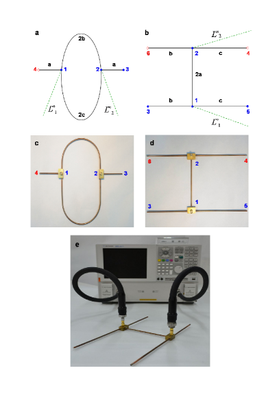
Figure 1: A pair of isoscattering quantum graphs and the pictures of two isoscattering microwave networks are shown in the panels (a)–(b) and (c)–(d), respectively. Using the two isospectral graphs, (a) with $n=4$ vertices and (b) with $n=6$ vertices, isoscattering quantum graphs are formed by attaching the two infinite leads $L^{\infty}_{1}$ and $L^{\infty}_{2}$ (green dashed lines). The vertices with Neumann boundary conditions are denoted by blue full circles while the vertices with Dirichlet boundary conditions by red open ones. The two isoscattering microwave networks with $n=4$ and $n=6$ vertices which simulate quantum graphs (a) and (b), respectively, are shown in the panels (c)–(d). The vertices of both networks are numbered, the numbers are colored (red/blue), that refers to the (Neumann/Dirichlet) boundary conditions at the vertices. The panel (e) shows the experimental setup used to measure the two-port scattering matrix $S(\nu)$ of the networks. In the experiment the vector network analyzer Agilent E8364B was used.

In order to test experimentally a negative answer to the modified Mark Kac’s question we consider two graphs shown in Fig. 1a and Fig. 1b. The graphs are isospectral Sawicki10 . The isoscattering graphs are obtained from them by attaching two infinite leads $L^{\infty}_{1}$ and $L^{\infty}_{2}$. Two corresponding microwave isoscattering networks constructed from microwave coaxial cables are shown in Figs. 1c and 1d. In order to preserve the same approximate size of the graphs in Fig. 1a and Fig. 1b and the networks in Fig. 1c and Fig. 1d, respectively, the lengths of the graphs were rescaled down to the physical lengths of the networks, which differ from the optical ones by the factor $\sqrt{\varepsilon}$, where $\varepsilon\simeq 2.08$ is the dielectric constant of a homogeneous material filling the space between the inner and the outer leads of the cables.

The graph in Fig. 1a consists of $n=4$ vertices connected by $B=4$ bonds. The valency of the vertices $1$ and $2$ reads $v_{1,2}=4$ (including leads) while for the other ones $v_{i}=1$. At the vertices with numbers $1,2$ and $3$ the Neumann vertex conditions are satisfied while for the vertex $4$ the Dirichlet condition is imposed. The second graph (see Fig. 1b) consists of $n=6$ vertices connected by $B=5$ bonds. At the vertices with numbers $1,2,3$ and $5$ we impose the Neumann vertex conditions, while for the vertices $4$ and $6$ we have the Dirichlet one.

Each system is described in terms of $2\times 2$ scattering matrix $S(\nu)$:

$$S(\nu)=\left(\begin{array}[]{cc}S_{1,1}(\nu)&S_{1,2}(\nu)\\ S_{2,1}(\nu)&S_{2,2}(\nu)\end{array}\right)\mbox{,}$$ (1)

relating the amplitudes of the incoming and outgoing waves of frequency $\nu$ in both leads.

Since the graphs presented in Fig. 1a and Fig. 1b are isoscattering the phases of the determinants of their scattering matrices should be equal for all values of $\nu$:

$$\mathrm{Im}\Bigl{[}\log\Bigl{(}\det\bigl{(}S^{(I)}(\nu)\bigr{)}\Bigr{)}\Bigr{]}=\mathrm{Im}\Bigl{[}\log\Bigl{(}\det\bigl{(}S^{(II)}(\nu)\bigr{)}\Bigr{)}\Bigr{]}\mbox{.}$$ (2)

In order to measure the two-port scattering matrix $S(\nu)$ we connected the vector network analyzer (VNA) Agilent E8364B to the vertices $1$ and $2$ of the microwave networks shown in Fig. 1c and Fig. 1d and performed measurements in the frequency range $\nu=0.01-1.7$ GHz. The connection of the VNA to a microwave network (see Fig. 1e) is equivalent to attaching of two infinite leads to quantum graphs which means Figs. 1a and 1b correctly describe the actual experimental arrangement.

The optical lengths of the bonds of the microwave networks had the following values:

$a=0.0985\pm 0.0005\mbox{ m, }$	$2a=0.1970\pm 0.0005\mbox{ m }$
$b=0.1847\pm 0.0005\mbox{ m, }$	$2b=0.3694\pm 0.0005\mbox{ m }$
$c=0.2420\pm 0.0005\mbox{ m, }$	$2c=0.4840\pm 0.0005\mbox{ m }$

At the frequency $\nu=1.7$ GHz the total optical length of the networks spans $5.96$ wavelengths of the microwave field. The uncertainties in the bonds’ lengths of the networks are due to the preparation of Neumann $v_{1,2}=4$ and Dirichlet vertices. In the case of the first ones the internal leads of the cables were soldered together while the Dirichlet vertices were prepared by closing the cables with brass caps to which the internal and external leads of the coaxial cables were soldered.

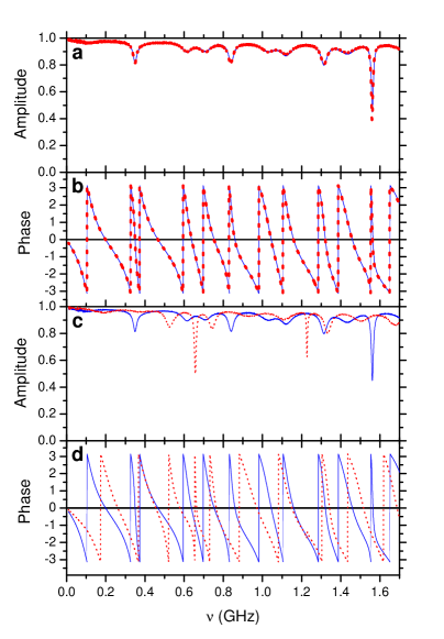
Figure 2: (a) The amplitude of the determinant of the scattering matrix obtained for the microwave networks with $n=4$ (blue solid line) and $n=6$ (red dotted line) vertices. (b) The phase of the determinant of the scattering matrix obtained for the microwave networks with $n=4$ (red dotted line) and $n=6$ (blue solid line) vertices. (c)-(d) The amplitudes and the phases of the determinants of the scattering matrices, respectively, measured for the network presented in Fig 1c (blue solid line) and the modified network Fig 1d (red dashed line), where the Neumann boundary condition in the vertex $5$ was replaced by the Dirichlet one. The results are presented in the frequency range $0.01-1.7$ GHz.

In the case of the microwave networks, where one deals with losses in the microwave cables Hul04 , not only the phase of the determinant $\phi=\mathrm{Im}\Bigl{[}\log\Bigl{(}\det\bigl{(}S(\nu)\bigr{)}\Bigr{)}\Bigr{]}$ but also the amplitude $|\det\bigr{(}S(\nu)\bigl{)}|$ as well gives an insight into the resonant structure of the system. The amplitudes and the phases of the determinants of the scattering matrices of the experimentally studied networks are shown in Fig. 2a and in Fig 2b, respectively. One sees that especially for lower frequencies $0.01-1.0$ GHz there is an excellent agreement between the results obtained for the both networks. The amplitudes of the determinants are so close to each other that the differences between them are hardly resolved in Fig. 2a. The phases of the determinants (see Fig. 2b) are in very good agreement in the full range of the investigated frequency $\nu=0.01-1.7$ GHz. In order to demonstrate the sensitivity of the spectral properties of the networks to the choice of the boundary conditions we compared the amplitudes and the phases of the determinants of the scattering matrices measured for the network presented in Fig 1c (blue solid line) and the modified network Fig 1d (red dashed line), where the Neumann boundary condition in the vertex $5$ was replaced by the Dirichlet one. One can easily see in Fig. 2c and Fig. 2d that such a modification causes a huge departure from the isoscattering properties.

Our experimental results strongly suggest the impossibility of ‘hearing’ of the shape of a graph or, in other words, that the question ”Are scattering properties of graphs uniquely connected to their shapes?” has to be answered in the negative.

Some small differences between the amplitudes appearing for $\nu>1$ GHz are due to different lengths of the networks. As it was discussed earlier the bonds’ lengths are known only with a certain accuracy. In order to check the influence of different bonds’ lengths we performed numerical calculations which took into account also the internal absorption of microwave cables Hul04 . We found that at certain realizations of the networks lengths the results, not shown here, mimic the behavior visible in Fig. 2a.

It was proven by the authors of Sawicki10 that the graphs considered in this paper have an additional important property, namely the scattering matrices of the graphs are conjugated to each other by the following transplantation relation:

$$S^{(II)}(\nu)=T^{-1}S^{(I)}(\nu)T\mbox{,}$$ (3)

where $T=\left(\begin{array}[]{cc}1&-1\\ 1&1\end{array}\right)$. It is worth noting that the matrix $T$ does not depend on the frequency and the equation (3) is valid for all values of $\nu$.

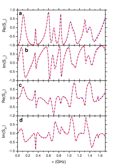
Figure 3: (a) The real and (b) imaginary parts of the matrix element $\tilde{S}^{(I)}_{1,1}(\nu)$ of the transformed scattering matrix (blue solid line) for the system with $n=4$ vertices. The obtained results are compared to the scattering matrix elements $S^{(II)}_{1,1}(\nu)$ of the graph with $n=6$ vertices (red dotted line). (c) The real and (d) imaginary parts of the matrix element $\tilde{S}^{(I)}_{2,1}(\nu)$ of the transformed scattering matrix (blue solid line) for the system with $n=4$ vertices. The results are compared to the scattering matrix element $S^{(II)}_{21}(\nu)$ of the graph with $n=6$ vertices (red dotted line). The results are presented in the frequency range $0.01-1.7$ GHz.

In order to check the transplantation relation expressed by equation (3) we transformed experimentally measured scattering matrix of the first network $\tilde{S}^{(I)}(\nu)=T^{-1}S^{(I)}(\nu)T$ and compared it to the scattering matrix of the second network $S^{(II)}(\nu)$. In Fig. 3 we present the results for the real and imaginary parts of $S_{1,1}$ and $S_{2,1}$ elements, respectively. The figure shows clearly that the transplantation relation for the real and imaginary parts of $S_{1,1}(\nu)$ and $S_{2,1}(\nu)$ elements works very well. Some small differences seen for $\nu>1$ GHz are caused, as previously, by small differences in the cables’ lengths. However, in general, the transformed scattering matrix of the first network $\tilde{S}^{(I)}(\nu)$ reconstructs very well the scattering matrix of the second one $S^{(II)}(\nu)$.

The considered microwave networks are obviously dissipative due to the absorption in the bonds. The loses are proportional to the total length of bonds, in our case the same for both networks. As it was shown in Hul04 loses can be effectively incorporated to the description by treating the wave number $k$ as a complex quantity with absorption-dependent imaginary part $\mathrm{Im}\Bigl{[}k\Bigr{]}$ and the real part $\mathrm{Re}\Bigl{[}k\Bigr{]}=2\pi\sqrt{\varepsilon}\nu/\textsc{c}$, where c is the speed of light in vacuum. On the other hand the authors of Sawicki10b proved that the transplantation formula (3) is satisfied also for complex $k$ (see p. A-152 in Sawicki10b ). It was thus reasonable to expect that the influence of dissipation on the presented results can be neglected and it was indeed the case. The above theoretical findings were also confirmed in the numerical calculations (not presented here) which showed that the internal absorption of the cables does not influence the transplantation relation (3). Consequently, the validity of the transplantation relation between the two-port scattering matrices could be experimentally demonstrated with such a good accuracy as in Fig. 3.

Summarizing, we investigated experimentally scattering properties of two microwave networks. We showed that the concept of isoscattering graphs was not only a theoretical idea but it could be also realized experimentally. We demonstrated that the microwave networks considered in the experiment are isoscattering, i.e., the phases and amplitudes of the determinant of the two-port scattering matrices are the same, within the experimental errors, for all the frequencies considered. In this way we strongly support a negative answer to the title question about possibility of connecting uniquely the shapes and scattering properties of graphs. In addition we checked the validity of the transplantation relation between the two-port scattering matrices of the two isoscattering microwave networks. It was shown that this relation allows to reconstruct the scattering matrix of each investigated network using the scattering matrix of the other one.

Our experimental setup can be successfully used to investigate properties of any quantum graph, also with highly complicated topology, see, e.g., Lawniczak2008 ; Lawniczak2010 ; Hul2011 . Here we showed that they are also relevant in the study of one of ’abstract’ but highly important mathematical problems of the spectral analysis showing a great research potential of quantum simulations based on microwave networks.

The authors thank R. Band for critical reading of the manuscript. This work was supported by the Ministry of Science and Higher Education grant No. N N202 130239.

References

- (1) M. Kac, Am. Math. Mon. 73, 1 (1966).
- (2) C. Gordon, D. Webb, and S. Wolpert, Invent. Math. 110, 1 (1992).
- (3) C. Gordon, D. Webb, and S. Wolpert, Bull. Am. Math. Soc. 27, 134 (1992).
- (4) T. Sunada, Ann. Math. 121, 169 (1985).
- (5) S. Sridhar and A. Kudrolli, Phys. Rev. Lett. 72, 2175 (1994).
- (6) Y. Okada, A. Shudo, S. Tasaki, and T. Harayama, J. Phys. A 38, L163, (2005).
- (7) B. Gutkin and U. Smilansky, J. Phys. A 34, 6061 (2001).
- (8) R. Band, O. Parzanchevski, and G. Ben-Shach, J. Phys. A 42, 175202 (2009).
- (9) O. Parzanchevski and R. Band, J. Geom. Anal. 20, 439 (2010).
- (10) R. Band, A. Sawicki, and U. Smilansky, J. Phys. A 43, 415201 (2010).
- (11) R. Band, A. Sawicki, and U. Smilansky, Acta Phys. Pol. A 120, A149 (2011).
- (12) S. Gnutzmann and U. Smilansky, Adv. Phys. 55, 527 (2006).
- (13) K.A. Dick, K. Deppert, M.W. Larsson, T. Märtensson, W. Seifert, L.R. Wallenberg, and L. Samuelson, Nature Mater. 3, 380 (2004).
- (14) K. Heo et al., Nano Lett. 8, 4523 (2008).
- (15) O. Hul, S. Bauch, P. Pakonski, N. Savytskyy, K. Życzkowski, and L. Sirko, Phys. Rev. E 69, 056205 (2004).
- (16) O. Hul, O. Tymoshchuk, S. Bauch, P.M. Koch, and L. Sirko, J. Phys. A 38, 10489 (2005).
- (17) M. Ławniczak, O. Hul, S. Bauch, P. Šeba, and L. Sirko, Phys. Rev. E 77, 056210 (2008).
- (18) M. Ławniczak, S. Bauch, O. Hul, and L. Sirko, Phys. Rev. E 81, 046204 (2010).
- (19) O. Hul and L. Sirko, Phys. Rev. E 83, 066204 (2011).