Horizontal flow fields observed in
Hinode G-band images

Abstract

Context. Emergence of magnetic flux plays an important role in the initiation of flares. However, the role of submerging magnetic flux in prompting flares is more ambiguous, not the least because of the scarcity of observations.

Aims. The flare-prolific active region NOAA 10930 offered both a developing $\delta$-spot and a decaying satellite sunspot of opposite polarity. The objective of this study is to characterize the photometric decay of the satellite sunspot and the evolution of photospheric and chromospheric horizontal proper motions in its surroundings.

Methods. We apply the local correlation tracking technique to a 16-hour time-series of Hinode G-band and Ca ii H images and study the horizontal proper motions in the vicinity of the satellite sunspot on 2006 December 7. Decorrelation times were computed to measure the lifetime of solar features in intensity and flow maps.

Results. We observed shear flows in the dominant umbral cores of the satellite sunspot. These flows vanished once the penumbra had disappeared. This slow penumbral decay had an average rate of 152 Mm² day^-1 over an 11-hour period. Typical lifetimes of intensity features derived from an autocorrelation analysis are 3–5 min for granulation, 25–35 min for G-band bright points, and up to 200–235 min for penumbrae, umbrae, and pores. Long-lived intensity features (i.e., the dominant umbral cores) are not related to long-lived flow features in the northern part of the sunspot, where flux removal, slowly decaying penumbrae, and persistent horizontal flows of up to 1 km s^-1 contribute to the erosion of the sunspot. Finally, the restructuring of magnetic field topology was responsible for a homologous M2.0 flare, which shared many characteristics with an X6.5 flare on the previous day.

Conclusions. Notwithstanding the prominent role of $\delta$-spots in flaring, we conclude based on the decomposition of the satellite sunspot, the evolution of the surrounding flow fields, and the timing of the M2.0 flare that the vanishing magnetic flux in the decaying satellite sunspot played an instrumental role in triggering the homologous M2.0 flare and the eruption of a small H$\alpha$ filament. The strong magnetic field gradients of the neighboring $\delta$-spot merely provided the vehicle for the strongest flare emission about 10 min after the onset of the flare.

1 Introduction

A theoretical description of flares has to explain their underlying cause and the origin of the various observed features (e.g., flare ribbons, loops, emissions across all wavelength regimes, and particle acceleration). Priest & Forbes (2002) review recent flare models–starting with some type of magnetohydrodynamic (MHD) catastrophe followed by magnetic reconnection–with an emphasis on three-dimensional models, which are required for a full appreciation of the dynamics in complex magnetic field topologies. Beyond modeling efforts, a wealth of new data became available by space missions such as RHESSI, Yohkoh, TRACE, and SoHO. Observations in the extreme ultra-violet (EUV) and in soft/hard X-rays revealed a plethora of transition region and coronal arcades and loops as summarized by Benz (2008), who discusses energetic and eruptive events as well as the nature of energy release and particle deposition. More recently, the relevant MHD processes such as flux emergence, formation of a current sheet, rapid dissipation of electric current, shock heating, mass ejection, and particle acceleration have been recounted by Shibata & Magara (2011).

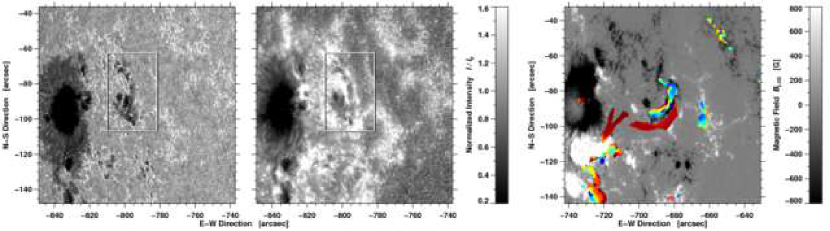
Figure 1: First calibrated G-band (left ) and Ca ii H (middle ) image in a 16-hour time-series of active region NOAA 10930 at 2:30 UT on 2006 December 7. The region in the white rectangle is the region-of-interest, i.e., a small satellite sunspot. SOT/NFI magnetogram (right ) captured at 18:46 UT on 2006 December 7. The rainbow-colored regions are the flare kernels derived from 32 Ca ii H images covering the M2.0 flare for 16 min from 18:47 UT to 19:03 UT. The time progresses from blue to red. A Big Bear Solar Observatory full-disk H$\alpha$ (Denker et al., 1999) image taken at 18:39 UT is used to trace a small filament (reddish colors), which consists of a V- and sickle-shaped region. The annotation of the axes refers to heliocentric coordinates given in seconds of arc.

Newly emerging flux has been linked to solar flares, whereas flares related to sunspot decay are not broadly discussed in literature. Simultaneous emergence and submergence of magnetic flux has been explored by Kálmán (2001) for the two (recurring) active regions NOAA 6850 (6891) and 7220 (7222). Based on X-ray observations no direct interaction of new and old magnetic flux was evident. However, flaring was observed for active region NOAA 6891 where only one magnetic polarity submerged. The magnetic field evolution was comparatively slow in these cases with time scales ranging from several hours to days. An intermediate case has been discussed by Wang et al. (2002), who observed an M2.4 flare associated with rapid penumbral decay (within a time period of just a few minutes) immediately after the flare, which was followed by the slow decay (three hours) of the remaining umbral core. The first phase of sunspot decay, i.e., rapid penumbral decay, has been established as an important signature of flare-related photospheric magnetic field changes (see e.g., Wang et al., 2004; Deng et al., 2005; Liu et al., 2005; Sudol & Harvey, 2005; Ravindra & Gosain, 2012). In our study of the flaring active region NOAA 10930, we focus on the gradual decay of a satellite sunspot and discuss its relationship to a developing $\delta$-spot of opposite polarity.

Active region NOAA 10930 was the first complex sunspot group producing X-class flares that was observed by the Japanese Hinode mission. The region was the source of the well-studied X3.4 solar flare on 2006 December 13 (e.g., Schrijver et al., 2008). For this highly active time period Tan et al. (2009) applied local correlation tracking (LCT) to study horizontal proper motions related to penumbral filaments in a rapidly rotating $\delta$-spot (Min & Chae, 2009). Both studies found twisted penumbral filaments, shear flows, sunspot rotation, and emerging flux at various locations within the active region. However, for the time just after the region rotated onto the solar disk, fewer studies were published, which mostly focused on the X6.5 flare on 2006 December 6 (e.g., Wang et al., 2012).

Balasubramaniam et al. (2010) described a prominent Moreton wave having an angular extent of almost 270^∘, which was initiated by the X6.5 flare. The radiant point of the Moreton wave appeared to be located at a small satellite sunspot to the west of the major sunspot, whereas X-ray, white-light, and G-band emissions were centered on the developing $\delta$-spot to the south. The strongest changes of the magnetic force also occurred at this location (cf., Fisher et al., 2012). Rapid penumbral decay and changes in the horizontal flow fields associated with the X6.5 flare were discussed by Deng et al. (2011). They observed the enhanced and sheared Evershed flow along the magnetic neutral line separating the main and $\delta$-spots. They concluded that the increased flow speed is not associated with new flux emergence in the active region. In the present study, we follow up the evolution of active region NOAA 10930 after the X6.5 flare leading up to a homologous M2.0 flare on 2006 December 7.

2 Observations

Table 1: Flare list for 2006 December 7 with starting, peak, and end times as well as flare sites in heliocentric coordinates and X-ray flare class.

Start Time	Peak Time	End Time	Position		X-Ray Class
03:32 UT	03:36 UT	03:39 UT	E766″	0S86″	C2.0
04:27 UT	04:45 UT	05:09 UT	E764″	S120″	C6.1
10:49 UT	11:48 UT	12:57 UT	E720″	S120″	C1.1
14:49 UT	15:15 UT	15:33 UT	E709″	S120″	C1.2
18:20 UT	19:13 UT	19:33 UT	E687″	S103″	M2.0

• Figure 3 provides a graphical representation of flare timing and the GOES X-ray flux. Data were provided by NOAA’s National Geophysical Data Center (NGDC).

Active region NOAA 10930 appeared on the eastern solar limb on 2006 December 5. The sunspot group was classified as a $\beta\gamma\delta$-region exhibiting a complex magnetic field topology, and it produced numerous C-, M-, and X-class flares. On 2006 December 7, we have analyzed 16 hours of data during the time period from 02:30 UT to 18:30 UT about eight hours after the X6.5 flare. The region was located at heliocentric coordinates E800″ and S85″ ($\mu=0.56$, where $\mu=\cos(\theta)$ is the cosine of the heliocentric angle $\theta$). The sequence with a cadence of 30 s is comprised of 1920 G-band and Ca ii H images (left and middle panels of Fig. 1) captured by the Solar Optical Telescope (SOT, Tsuneta et al., 2008) on board the Japanese Hinode mission (Kosugi et al., 2007). We dropped every second image from the time-series because a cadence of 60 s is sufficient for measuring horizontal proper motions. A SOT/NFI magnetogram (right panel of Fig. 1) serves as reference to illustrate the magnetic configuration of NOAA 10930, which is later used in the discussion of the M2.0 flare at 18:47 UT (see Sect. 3.5). The G-band and Ca ii H images are $2\times 2$-pixel binned with an image scale of 0.11″ pixel^-1. Thus, the $1024\times 1024$-pixel images have a FOV of $111\arcsec\times 111\arcsec$. After basic data calibration, the images were corrected for geometrical foreshortening and resampled onto a regular grid of 80 km $\times$ 80 km (see Verma & Denker, 2011).

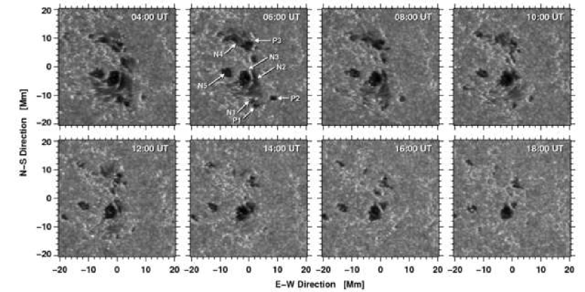
Figure 2: Time-series of calibrated and geometrically corrected G-band images of the satellite sunspot in active region NOAA 10930 depicting various stages of its decay. The labels N and P refer to magnetic features with negative and positive polarities, respectively.

The region-of-interest (ROI) with a size of 40 Mm $\times$ 40 Mm was centered on a small decaying sunspot in the western part of the active region (see the white rectangular region in Fig. 1 before geometrical correction). This satellite spot significantly evolved over the course of 16 hours. Accompanied by C- and M-class flares (Tab. 1), the penumbra of the small spot almost completely vanished. The X-ray flux over three days as measured by the Geostationary Operational Environmental Satellite (GOES) is shown in Fig. 3, where the shaded region indicates the 16-hour observing period. Before measuring horizontal proper motions, the signature of the five-minute oscillation was removed from the images by using a three-dimensional Fourier filter with a cut-off velocity of 8 km s^-1, which corresponds roughly to the photospheric sound speed. To scrutinize flow fields associated with slow penumbral decay and its relationship to flaring, we used the LCT method described in Verma & Denker (2011).The technique computes cross-correlations over $32\times 32$-pixel regions with a Gaussian sampling window having a FWHM of 15 pixels (1200 km) corresponding to the typical size of a granule.

3 Results

In the following, we will describe the decay of the satellite sunspot, compute the photometric decay rates of its umbra and penumbra, and study the impact of the decay process on photospheric and chromospheric horizontal flows. The photometric observations together with a temporal analysis of the flow maps yields estimates of decay times of various solar features. Finally, we relate these findings to an M2.0 flare, which occurred towards the end of the time-series.

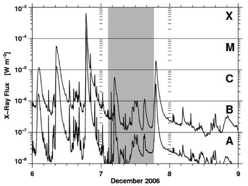
Figure 3: One-minute GOES-11 X-ray flux on 2006 December 6–9 obtained in the 0.05–0.40 nm (bottom ) and 0.1–0.8 nm (top ) energy channels. The shaded region indicates the time interval of 16 hours covered by Hinode data analyzed in the present study.

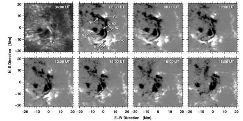
Figure 4: Time-series of calibrated and geometrically corrected Hinode/NFI magnetograms corresponding to the G-band images in Fig. 2. The line-of-sight magnetic field $B_{LOS}$ is displayed in the range of $\pm 800$ G as in Fig. 1.

3.1 Morphology

The temporal evolution of the decaying satellite sunspot is shown at two-hour intervals in Fig. 2. Note that after geometric correction the axis labels no longer refer to heliographic coordinates on the solar disk. They are more readily provided for easier identification and comparison of intensity or flow features. As a convenient reference to photometric and magnetic components of the satellite spot, we provided numbered labels P and N in Figs. 2 and 4 referring to positive- and negative-polarity features, respectively. Initially, the ROI contains a few umbral cores with rudimentary penumbrae, which are embedded in regions covered by G-band bright points. The strongest umbral core N3 is located close to the center of the ROI, where it is separated from an elongated umbral core N2 by a faint light-bridge. The southern side of the light-bridge flares out in a strand of penumbral filaments, which wind around the strong umbral core. Non-radial penumbral filaments are indicative of shear flows (e.g., Denker et al., 2007; Jiang et al., 2012). These filaments became significantly weaker in response to a C6.1 flare at 04:45 UT, which can be considered as a form of a ‘rapid’ penumbral decay (Wang et al., 2004; Liu et al., 2005), however, in this case observed very localized and at high spatial resolution. In addition to shear flows, we observed an umbral core N5 drifting away eastward from the dominant umbral core N3. The separation of these umbral cores grew by 6 Mm over the course of 14 hours, i.e., the separation speed is about 120 m s^-1. Three small, 1-Mm wide pores of positive and negative polarity (P1, P2, and N1) are located to the south of the strong umbral core. All three pores disappeared by the end of the time-series. In addition, penumbral regions started decaying across the entire ROI at about 10:00 UT. At 12:00 UT only weak penumbral signatures were present so that only scattered pores were left by 14:00 UT. This period of ‘slow’ penumbral decay was accompanied by several B-class flares and a C1.1 flare at 11:48 UT.

In addition to the photometric evolution shown in Fig. 2, we also trace in Fig. 4 the reduction of magnetic complexity in the satellite sunspot, which is based on Hinode NFI magnetograms taken in the photospheric Fe i $\lambda$630.25 nm line. The Stokes-$V/I$ magnetograms have $1024\times 1024$ pixels and an image scale of 0.16″ pixel^-1. From the Stokes-$V$ and $I$ signal the approximate line-of-sight magnetic field was calculated as

$$B_{\mathrm{LOS}}=-\frac{C_{V}}{0.798C_{I}}\times 10^{4}\leavevmode\nobreak\ \mathrm{Mx\leavevmode\nobreak\ cm}^{-2}$$ (1)

given in Isobe et al. (2007). We scaled the magnetograms displayed in Figs. 1 and 4 using this relation. However, no attempt was made to translate the LOS magnetic fields into the field component $B_{z}$ normal to the solar surface. These data were only corrected for geometrical foreshortening and carefully matched to the G-band images. Unfortunately, no magnetograms were available until 06:30 UT so that we substituted a Ca ii H image in the first panel of Fig. 4, and we had to resort to a magnetogram taken about 30 min later than the G-band companion in the second panel. Note that the proximity of the active region to the solar limb casts doubt on simply associating the sign of the circular polarization with the sign of the magnetic fields component that is normal to the solar surface. In particular, we observe in the NFI magnetograms at the begining of the time-series apparent polarity reversals in limbward penumbral regions for both the major and satellite sunspots, which are clearly related to the close to horizontal magnetic field lines in these regions.

At the beginning of the time-series, the satellite sunspot was much more complex than either the main spot or the developing $\delta$-spot. Four magnetic features with negative polarity and three features with positive polarity play a role in the decay of the satellite sunspot. Over a period of 16 hours the complexity of the magnetic fields was much reduced. The dominant umbra N3 is separated by a light-bridge from a curved and elongated umbra N2. Brightening of the small-scale features along the light-bridge around 06:00 UT can be taken as an indication that convection penetrates the strong magnetic fields, thus, contributing to the decay of the satellite spot. During this decay the satellite sunspot slowly rotates counterclockwise ($\approx 3.6\mbox{${}^{\circ}$}$ h^-1) as can be seen in Fig. 3 using the light-bride as a tracer. This slow rotation adds up to more than 50^∘ over the course of the observations.

The core of the satellite spot, i.e., N2, N3, and the light-bridge, survive until the end of the time-series. The curved, non-radial penumbral filaments associated with this core can be traced not just in intensity but also in magnetograms. The observed alternating polarities of the filaments could just be projection effects of nearly horizontal magnetic fields. This effect is likewise visible at the limb-side penumbra of the main spot and for the magnetic element N5. Despite of its strong proper motion (see above), the photometric and magnetic decay of N5 is slow. Only towards the end of the time-series the pore starts to break up. A conspicuous, bright umbral dot appears in the center of the pore around 18:00 UT. Together with two protrusions from the periphery of the pore, it forms a structure like a light-bridge indicating further erosion of the pore. This erosive process is easier to follow in intensity than in the magnetic field evolution, where N5 remains compact.

Two small pores N1 and P1 are located to the south of the dominant umbra. Magnetic cancellation characterizes the evolution of this small magnetic bipole. As the minority polarity N1 disappeared earlier than P1. At 10:00 UT only P1 was left. In general, the photometric decay proceeds faster than the decline of the magnetic flux. This also holds true for the third small pore P2, which survived somewhat longer than P1 and can still be detected as a tiny magnetic knot in the G-band image at 18:00 UT.

To the east of a small umbral core P3 we observe a rudimentary penumbra of opposite polarity, which had dissolved by 14:00 UT. The underlying magnetic field N4 of the rudimentary penumbra was elongated stretching over a distance of about 18 Mm connecting to the also elongated umbral core N2. Together, N2 and N4 define the magnetic neutral line of the satellite sunspot, with strong positive fields at the extremities to the south (P1 and P2) and north (P3). The slow cancellation of flux associated with P3 continues over the 16-hour period and results in long-lived flow features in the decorrelation maps (see Sect. 3.4).

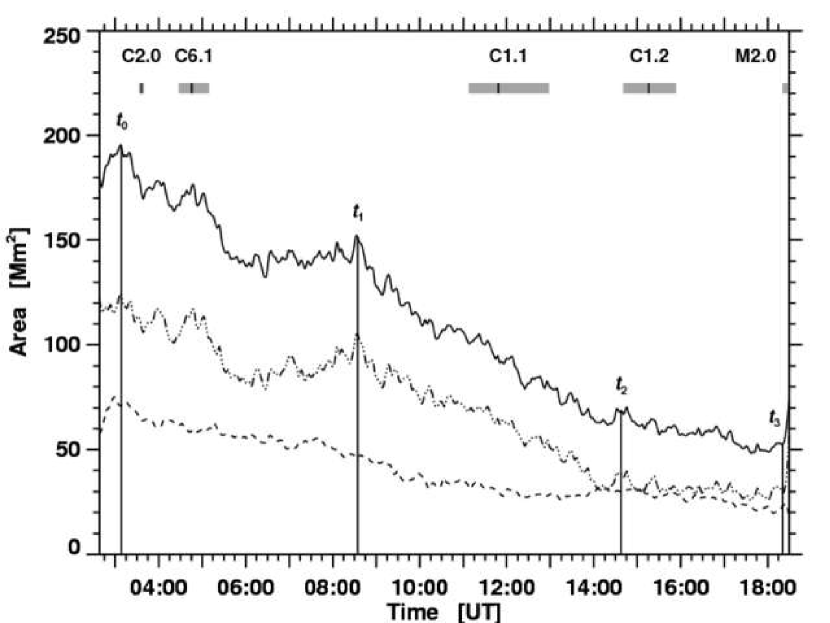
Figure 5: Temporal evolution of the area covered by active region NOAA 10930 over the 16-hour period from 02:30–18:30 UT. The area enclosed by umbral cores and pores is displayed with a dashed line. The dash-dot-dotted line refers to the penumbra, whereas the solid line denotes the total area. The times $t_{0}$, $t_{1}$, $t_{2}$, and $t_{3}$ delimit time intervals over which the linear photometric decay rates were computed (see Tab. 2). The gray bars depict the duration of flares (Tab. 1), where the thin black line marks the peak time for flares.

Table 2: Decay rates [Mm² day^-1] of penumbra, umbra, and the entire satellite sunspot (pores, umbrae, and penumbrae) for four time intervals.

Feature	Decay rate [Mm2 day-1] for four time intervals
	$t_{0}-t_{1}$	$t_{1}-t_{2}$	$t_{2}-t_{3}$	$t_{0}-t_{3}$
Penumbra	$130.2$	$244.2$	$31.3$
Umbra	0$86.4$	0$68.4$	$67.9$	0$73.7$
Spot	$216.6$	$312.6$	$99.3$	$225.8$

• The time intervals are $t_{0}$= 03:07 UT, $t_{1}$= 08:36 UT,
  $t_{2}$= 14:46 UT, $t_{3}$= 18:20 UT.

3.2 Decay rates

We used morphological thresholding for discerning various solar features in intensity. Images were normalized using eight quiet Sun regions evenly spread over the time-series. Thus, a weak trend in mean intensity (center-to-limb variation related to solar rotation) was removed from the data. We used a fixed intensity threshold of $I_{\mathrm{mag}}<0.85$ for strong magnetic features and an adaptive threshold for G-band bright points (see Verma & Denker, 2011), which is given as

$$I_{\mathrm{bp}}=1.15+0.2(1-\mu)\,.$$ (2)

The umbrae were identified using a fixed threshold of $I_{\mathrm{dark}}=0.6$, while sunspot penumbrae cover intermediate intensities from $I_{\mathrm{mag}}$ to $I_{\mathrm{dark}}$, and granulation lies between $I_{\mathrm{mag}}$ to $I_{\mathrm{bp}}$. The adaptive threshold was used as a first-order approximation to take into account the center-to-limb variation of G-band bright points because they exhibit an enhanced contrast near the solar limb. The thresholding algorithm also allows us to compute the area for different solar features. The algorithm provides in general a good estimate of the area except for a few small features and towards the end of the sequence, when only pores are left, for which the borders are erroneously classified as penumbra. If many small pores are present, then their periphery with intensities like penumbra can be significantly larger than the cores of the pores themselves.

The curves in Fig. 5 represent the temporal evolution of areas subsumed by umbral cores/pores, penumbrae, and the entire satellite spot (sum of pores, umbra, and penumbra). At the beginning of the time-series, the area of all magnetic features was about 200 Mm², of which approximately two thirds were classified as penumbra and the remaining third corresponded to umbral cores/pores. By the end of the time-series only the later features stayed on covering little over 50 Mm², i.e., only one quarter of the area intially covered by the strong magnetic features. The features’ decay rates were computed using linear regression. We divided the time-series into four time intervals $t_{0}-t_{1},t_{1}-t_{2},t_{2}-t_{3},$ and $t_{0}-t_{3}$, because the penumbral decay curve has two peaks at t₀ and t₁, and the penumbra had completely vanished at $t_{2}$. The time $t_{3}$ was chosen just eight images before the end of the time-series so that artifacts from the subsonic filtering become negligible, and it marks the onset of the M2.0 flare.

Slow penumbral decay is the distinctive feature of the satellite sunspots’s temporal evolution. Table 2 provides the respective photometric decay rates for the above mentioned time intervals. The penumbral decay rate significantly increases from $t_{0}$ – $t_{1}$ to $t_{1}$ – $t_{2}$ almost doubling its value to 244.2 Mm² day^-1. A linear regression might not be the best choice for the penumbral decay rate (130.2 Mm² day^-1) during the first time interval because there is a sudden decay in the area after the C6.1 flare at 04:45 UT. During the time interval $t_{2}$ – $t_{3}$ the penumbral area decayed by 4.7 Mm² in 3.6 h, which corresponds to a decay rate of 31.3 Mm² day^-1. However, this is just an artifact of the intensity thresholding algorithm used in classifying penumbral areas, which erroneously labels the boundaries of pores as penumbra. The 1-$\sigma$ uncertainties for the decay rates are about 2.5 Mm² day^-1.

Therefore, computing a penumbral decay rate for the entire time period $t_{0}$ – $t_{3}$ is not meaningful. The umbral decay rates do not vary much. The overall value of 73.7 Mm² day^-1 during $t_{0}$ – $t_{3}$ represents closely the decay rates for the shorter intervals. Hence, the penumbra decayed three time faster as the umbral cores. The decay rate of the spot is just the sum of the umbral and penumbral decay rates. The overall spot decay rate in current study (225.8 Mm² day^-1 for $t_{0}$–$t_{3}$) is well within the range of previously reported values, e.g., Bumba (1963) found a decay rate of 180 Mm² day^-1 for non-recurrent groups. Spot decay rates in other studies range from 10–125 Mm² day^-1 (e.g., Moreno-Insertis & Vazquez, 1988; Martínez Pillet et al., 1993; Hathaway & Choudhary, 2008).

3.3 Flow fields in photosphere and chromosphere

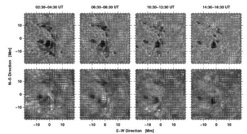
Figure 6: Horizontal flow fields averaged over two hours are depicted as arrows overlaid on geometrically corrected G-band (top ) and Ca ii H (bottom ) images of four time-series. The arrows indicate magnitude and direction of the horizontal proper motions. Arrows with a length corresponding to the grid size indicate velocities of 0.5 km s^-1.

Table 3: Parameters describing horizontal proper motions for various solar features based on the four G-band and Ca ii H time-series with $\Delta T=2$ h and $\Delta t=60$ s for four time-series shown in Fig. 6.

		$\bar{v}$	$v_{\mathrm{med}}$	$v_{10}$	$v_{\mathrm{max}}$	$\sigma_{v}$
Feature	Image Type	[km s-1]	[km s-1]	[km s-1]	[km s-1]	[km s-1]
All	G-Band	$0.33$	$0.29$	$0.63$	$1.46$	$0.21$
	Ca ii H	$0.35$	$0.28$	$0.69$	$2.31$	$0.25$
Granulation	G-Band	$0.35$	$0.31$	$0.65$	$1.43$	$0.21$
	Ca ii H	$0.36$	$0.30$	$0.71$	$2.31$	$0.25$
Penumbra	G-Band	$0.28$	$0.24$	$0.51$	$1.22$	$0.19$
	Ca ii H	$0.30$	$0.24$	$0.60$	$1.36$	$0.21$
Umbra	G-Band	$0.20$	$0.19$	$0.33$	$0.60$	$0.10$
	Ca ii H	$0.30$	$0.23$	$0.66$	$1.19$	$0.23$
Bright Points	G-Band	$0.18$	$0.17$	$0.32$	$0.71$	$0.10$
	Ca ii H	$0.19$	$0.18$	$0.32$	$0.82$	$0.10$

For computing the characteristic parameters of the penumbral flow field we neglected the last time interval $t_{2}$–$t_{3}$, since by that time the penumbra had decayed and the features detected as penumbra were just artifacts of the thresholding algorithm. The time period $t_{0}$–$t_{2}$ was excluded from calculating Ca ii H flow parameters of the umbra, since motions along post-flare loops resulted in high flow speeds.

The two-hour averaged LCT flow maps shown in Fig. 6 were computed using the 16-hours time-series of Hinode G-band and Ca ii H images. We used the satellite sunspot as a reference and aligned all images in time-series accordingly. These flow maps provide insight into horizontal proper motions in the photosphere and chromosphere. We quantified horizontal proper motions for various solar features (e.g., bright points, granulation, sunspot penumbrae, and strong magnetic features) by applying morphological and adaptive thresholds to G-band images (see Sect. 3.1). We applied the same indexing to the Ca ii H flow maps to have an one-to-one correspondence comparing photospheric and chromospheric flow fields, while neglecting morphological differences. We calculated the mean $\bar{v}$, median $v_{\mathrm{med}}$, maximum $v_{\mathrm{max}}$, $10^{\mathrm{th}}$ percentile $v_{10}$, and standard deviation $\sigma_{v}$ of the horizontal flow speeds (see Tab. 3). The standard deviation in the flow speed refers to the variance in the data rather than to a formal error. Typical flow characteristics of solar features were reported by Verma & Denker (2011), who also presented values for other time intervals $\Delta T$ and cadences $\Delta t$. Here, we computed the flow parameters for four time-series with $\Delta T=2$ h and afterwards averaged them. The average flow parameters of the various solar features are within the expected ranges except for granulation where $\bar{v}=0.35\pm 0.21$ km s^-1, which is lower than the value of $\bar{v}=0.47\pm 0.27$ km s^-1 mentioned in Verma & Denker (2011). However, the granular flow speed could be lower because of the presence of strong magnetic flux concentrations. Regions of granulation, which are not in close proximity to strong magnetic fields, often showed strong divergence centers, e.g., in the south-west corner of the FOV towards the end of the time-series. In general, photospheric and chromospheric flow parameters are virtually the same. The only notable dissimilarity between the G-band and Ca ii H flow maps relates to post-flare loops straddling the dominant pore N3. These loops are most prominent in Ca ii H images and result in strong flows of more than 1.14 km s^-1 (Fig. 6: 06:30–08:30 UT). The signature of these post-flare loops is still visible at later time periods. However, the associated flows are much weaker. Other than that differences in the frequency distributions exist only for the high-speed tail, i.e., the maximum speed $v_{\mathrm{max}}$ and to a lesser extend the 10^th percentile speed $v_{10}$.

In the two-hour averaged LCT flow maps the overall impression of flow vectors for G-band and Ca ii H images is indistinguishable. The flow patterns around the satellite sunspot are different from regular sunspots (e.g., Balthasar & Muglach, 2010) because of its non-radial penumbra and location within a complex active region. The most intriguing feature in the G-band flow maps is the anticlockwise spiral motion around the dominant umbral core N3. The light-bridge between N2 and N3 marks the location of shear flows, where stronger flows ($\approx 0.45$ km s^-1) linked to the elongated umbra N2 move past weaker flows($\approx 0.17$ km s^-1) spiraling around the dominant umbra N3. The spiral motion and shear flows were most conspicuous in the first flow map (02:30–04:30 UT) but faded out once the penumbra had decayed. Strong outward motions were present at the outer tips of penumbral filaments associated with N3 and P3 in the northern part of the FOV. These strong outward motions associated with P3 continue to exist until the end of the time-series and appear as long-lived features in the decorrelation maps of the flow speed (see Sect. 3.4).

3.4 Decorrelation times

The lifetime of solar features can be estimated by selecting a reference map at an instance $t_{i}$ and by computing how consecutive maps decorrelate with time. As put forward by Welsch et al. (2012), we computed linear Pearson and rank-order Spearmann correlation coefficients for G-band intensity and the corresponding horizontal flow speed. The flow speed maps were computed as sliding one-hour averages centered on each point in time $t_{i}$. Pearson’s correlation coefficient $\rho$ measures the strength of a linear dependence of two variables $x$ and $y$, and is computed by dividing the covariance of the two variables by the product of their standard deviations:

$$\rho=\frac{\displaystyle\sum_{i=1}^{N}\left(x_{i}-\bar{x}\,\right)\left(y_{i}-\bar{y}\,\right)}{\displaystyle\sqrt{\sum_{i=1}^{N}\left(x_{i}-\bar{x}\,\right)^{2}\cdot\sum_{i=1}^{N}\left(y_{i}-\bar{y}\,\right)^{2}}}$$ (3)

$$\mathrm{with}\;\,\bar{x}=\frac{1}{N}\sum_{i=1}^{N}x_{i}\;\,\mathrm{and}\;\,\bar{y}=\frac{1}{N}\sum_{i=1}^{N}y_{i}\,.$$

The Spearman correlation coefficient $r_{s}$ is similarly defined as the Pearson correlation coefficient between two ranked variables $\mathrm{r}(x)$ and $\mathrm{r}(y)$. We used an IDL algorithm based on the recipe provided in Press et al. (1992):

$$r_{s}=\frac{\displaystyle\sum_{i=1}^{N}\left(\mathrm{r}(x_{i})-\overline{\mathrm{r}(x)}\,\right)\left(\mathrm{r}(y_{i})-\overline{\mathrm{r}(y)}\,\right)}{\displaystyle\sqrt{\sum_{i=1}^{N}\left(\mathrm{r}(x_{i})-\overline{\mathrm{r}(x)}\,\right)^{2}\cdot\sum_{i=1}^{N}\left(\mathrm{r}(y_{i})-\overline{\mathrm{r}(y)}\,\right)^{2}}}$$ (4)

$$\mathrm{with}\;\,\bar{x}=\frac{1}{N}\sum_{i=1}^{N}\mathrm{r}(x_{i})\;\,\mathrm{and}\;\,\bar{y}=\frac{1}{N}\sum_{i=1}^{N}\mathrm{r}(y_{i})\,.$$

The 16-hour time-series was divided into two parts. The first eight-hour time-series covers the phase of penumbral decay, whereas towards the second half the penumbra had already vanished. Autocorrelation functions $r_{s}(t)$ were computed for intensity and flow maps over circular areas with a diameter of about 5 Mm and for lag times of up to 300 min. We used 16 and 10 reference frames for the intensity and speed maps, respectively. The number of reference frames had to be reduced to 10 in case of the flow maps because of the 60-minute sliding average. We averaged the autocorrelation functions to have different instances of surface features contributing to our sample. In both cases, the averages are based on 460 min of data, i.e., either $16\times 10+300$ min or $10\times 10+300+60$ min, where the last term results from the sliding averages. The thus averaged autocorrelation functions are fitted with decaying exponential functions.

$$r_{s}(t) = \Big{[}r_{s}\big{(}f(t_{0}),f(t_{1})\big{)},\;r_{s}\big{(}f(t_{0}),f(t_{2})\big{)},\;\ldots$$

$$\ldots,\;r_{s}\big{(}f(t_{0}),f(t_{n-1})\big{)},\;r_{s}\big{(}f(t_{0}),f(t_{n})\big{)}\Big{]}$$

$$\approx \exp\left(-\frac{1}{\tau}t^{\gamma}\right)\,,$$

where the constants $\tau$ and $\gamma$ are derived from a least-squares fit to the measured $r_{s}(t)$. The function $f(t)$ is either an intensity or a horizontal flow speed map. The lifetimes (or decorrelation times) were calculated for $r_{s}(t)=1/2$, i.e.,

$$t_{\nicefrac{{1}}{{2}}}=(\tau\ln 2)^{\nicefrac{{1}}{{\gamma}}}\,.$$ (6)

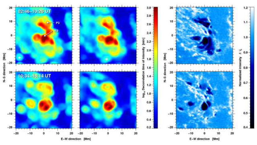
Figure 7: Decorrelation times computed using the linear Pearson (left) and Spearman’s rank order (middle) correlation coefficients for the intensity of G-band images. The time-series was divided into two parts from 02:46–10:26 UT (top) and 10:34–18:14 UT (bottom). Average G-band images for these time intervals (right) clearly show the penumbral decay of the satellite sunspot.

The case $\gamma=1$ corresponds to a simple exponential decay and $\tau$ would simply refers to the lifetime of the feature. This is the standard approach determining lifetimes of solar granulation but this simple decay law no longer holds in the presence of (strong) magnetic fields. Using also $\gamma$ as a free fit parameter results in a much improved $\chi^{2}$-statistics independent of the magnetic environment. If $\gamma\neq 1$, then $\tau$ can no longer be interpreted as lifetime. Therefore, we chose Eqn. 6 to determine how long solar features last because it removes the entanglement of $\tau$ and $\gamma$ by emphasizing the quality of the fit.

A more detailed analysis shows that $\gamma\approx 1$ in regions with granulation and $\gamma\approx 1/2$ in sunspots are representative values for the autocorrelation functions of intensity features. The autocorrelation functions of flow features are characterized by $\gamma\approx 3/2$ with no major differences between sunspots and granulation. However, the exponent can approach $\gamma\approx 3$ for some long-lived features, e.g., stationary G-band bright points. In these cases, the $\tau$ values become very large and can no longer be interpreted as a lifetime.

In Figs. 7 and 8, we depict the decorrelation-time maps for the intensity and flow speed, respectively. Linear and rank-order correlations qualitatively produce the same decorrelation times. Our type of presentation differs from Welsch et al. (2012) because our decorrelation times were computed either for each pixel in the FOV (Pearson’s $\rho$) or for a $4\times 4$-pixel grid (Spearman’s $r_{s}$). The coarser sampling is necessitated because of the computational overhead in ranking the variables. These maps were then smoothed by a Gaussian with a FWHM of 1200 km. We inferred from the decorrelation maps of the intensity that the magnetic features have longer lifetimes than granulation, which is expected.

Regions of granulation can be extracted from the average G-band images shown in the right panels of Fig. 7, where they correspond to the dark blue regions to the west of the satellite sunspot. Typical granular lifetimes derived from the linear and rank-order decorrelation maps are about 3.1 min and 4.6 min, respectively. In the rank-order case, we find a standard deviation of the frequency distributions of about 1 min. Because of a pronounced tail towards longer lifetimes, the standard deviation of the linear case is much higher. However, the median is close to 3 min in both cases. There is no significant difference in the granular lifetimes during the first and second halves of the time-series. Our findings are in good agreement with the original work of Bahng & Schwarzschild (1961) and match accurately the findings of Title et al. (1989).

G-band bright points show two types of behavior: either they remain stationary as at the supergranular boundary at the western periphery of the FOV or they stream away from the satellite sunspot towards the main spot. In the long-duration G-band images the bright point coalesce into strands indicating preferential paths taken by small-scale magnetic features. Similar motion patterns were observed for the moat flow of decaying sunspot (Verma2012). However, thread-like concentrations of magnetic field were also observed by Strous et al. (1996) for an emerging active region. Thus, preferential paths for the migration of small-scale magnetic elements might be a common property of flux emergence, removal, and dispersal. The factor that G-band bright points being either stationary or moving does not have an impact on their lifetimes. The light-blue to turquoise colors denote lifetimes of about 35 min in linear and 25 min in rank-order decorrelation maps. The distributions in both cases have a pronounced high-lifetime tail. Note that individual, long-lived, and stationary G-band bright points can create artifacts, which appear as disk-shaped features (e.g., marked with white $+$ in Fig. 7) in the smoothed decorrelation maps because as long as they are fully contained in the circular correlation window, their presence outweighs any other contribution to the correlation function.

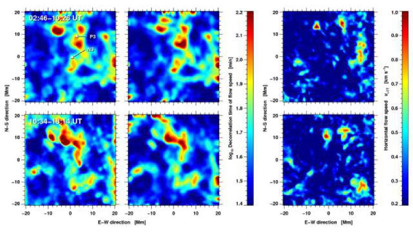
Figure 8: Decorrelation times computed using the linear Pearson (left) and Spearman’s rank order (middle) correlation coefficients for the horizontal flow speed. The time-series was divided into two parts from 02:46–10:26 UT (top) and 10:34–18:14 UT (bottom). Average flow speed maps (right) show several small regions with enhanced flows in the vicinity of long-lasting flow features.

The typical lifetime of strong magnetic features (pores, umbrae, and penumbrae) are about 200 min and 235 min using linear and rank-order correlations. There is virtually no difference in the respective distributions of magnetic features, except that the area covered by extremely long-lived feature (lifetimes $>$ 500 min) is moderately higher (1.8 Mm²) in case of rank-order correlations as compared to linear correlations (1.2 Mm²). The photometric decay of the satellite sunspot also leaves its mark in the decorrelation maps. The area covered by features living longer than 100 min decreased from 160 Mm² to 80 Mm², while in parallel the complexity of the long-lived features reduced. The lifetime in the vicinity of the umbral core P3 was about 300 min during the first half of the time-series. In the second half erosion of the rudimentary penumbra and slow cancellation of magnetic flux near P3 led to significantly shorter lifetimes (about 100 min) in that region. The only conspicuous feature that remained in the latter decorrelation map is a compact oval region associated with the dominant umbral core N3. In two small kernels with an area of about 2 Mm² the lifetime exceeds 1000 min.

Decorrelation maps of the flow speed are presented in Fig. 8. The right panels show the averaged, long-duration flow maps. Flow speeds are suppressed in regions containing strong and weak magnetic fields. Typical values are $0.24\pm 0.15$ km s^-1, where the standard deviation refers to the variance within the region covered by the satellite sunspot and the surrounding G-band bright points. Higher flow speeds ($0.52\pm 0.11$ km s^-1) are encountered in quieter areas. In particular in proximity to supergranular boundaries near the western periphery of the FOV, flow speeds approaching 1 km s^-1 are measured. For example, a strong divergence region (see Fig. 6 at time periods 10:30–12:30 UT and 14:30–16:30 UT) becomes apparent in the lower-right corner of the FOV in the second half of the time-series.

Two small flow kernels of about 1 Mm² possessing high-speed values approaching 1 km s^-1 are related to the decay of the rudimentary penumbra near the umbral core P3. They are related to slow flux cancellation in that region. These flow kernels also leave an imprint in the decorrelation maps. Note that the logarithmic scale of the decorrelation times significantly differs for G-band intensities and horizontal flow speeds. Surprisingly, the lifetimes associated with the dominant umbral core N3 are much lower than the ones for P3, i.e., horizontal flows are more persistent near P3. Thus, flows contribute to the decay of the satellite sunspot most noticeably in regions with weaker and less compact magnetic fields. Persistent flows have lifetimes typically above 80 min and survive up to 160 min. The frequency distributions of flow lifetimes derived from linear and rank-order decorrelation maps are virtually same. In both cases, the distributions are broad and do not have a high-velocity tail. Comparing Figs. 7 and 8, a higher fine-structure contents becomes immediately apparent, which might be explained by the shorter lifetimes of horizontal flow patterns.

3.5 Homologous M2.0 flare

An M2.0 flare started in active region NOAA 10930 at 18:20 UT towards the end of the time-series. Time-resolved Ca ii H flare kernels are shown in the right panel of Fig. 1. The color-coded flare kernels are based on images with the full cadence of 30 s. The first indications of this two-ribbon flare were associated with the remnants of the negative polarity features around N2 and N3 in the satellite sunspot. The second ribbon is located some 10–15 Mm away in a network region to the west with positive polarity. Flare brightenings related to the $\delta$-spot appear delayed by a few minutes. Furthermore, remote brightenings appear in a negative-polarity Ca ii H plage region towards the north-west. A small filament above the neutral line formed by the remnants of N2/N3 and P1/P2 erupted during the flare. The location of this filament was extracted from BBSO H$\alpha$ full-disk images and carefully matched with the magnetogram of Fig. 1.

The X6.5 flare on 2006 December 6 was also a two-ribbon flare. Here, the flare ribbons were located inside the umbra of the main spot and along the neutral line separating the main and $\delta$ spots. A filament located above this neutral line (see F1 in Fig. 11 of Balasubramaniam et al., 2010) erupted as a result of the flare and produced an impressive Moreton wave. The latter flare ribbon extended all the way to the satellite sunspot, which at that time was still connected to the main spot by a wide band of penumbral filaments. Rapid penumbral decay initiated by the X6.5 flare characterize this penumbral region. Deng et al. (2011) find no indications for flux emergence in this regions but attribute the initiation of the flare to (shear) flows along the magnetic neutral line, which were enhanced just before the onset of the flare. The rapid penumbral decay within the band connecting main and satellite sunspots (Wang et al., 2012) also marks the beginning of demise of the satellite sunspot.

Even though being separated by more than one order of magnitude in X-ray flux, the X6.5 and M2.0 flare share a variety of traits, so that they can be considered as homologous flares: both are two ribbon flares, filament eruption are observed in both cases, the reconfiguration of the magnetic field topology involves the satellite sunspots, and flux removal rather than emergence is a decisive mean in the flare process.

While rapid penumbral decay is a characteristic of the X6.5 flare, it only plays a very localized role in the M2.0 flare, where slow penumbral decay is the most prominent feature. Even though Moreton waves have been observed for M-class flare (Warmuth et al., 2004a, b), the absence of a wave for the M2.0 flare does not preclude the characterization of X6.5 and M2.0 flares as homologous. In particular, considering that Balasubramaniam et al. (2010) associate the radiant point, i.e., the origin of the Moreton wave more closely with the satellite sunspot, whereas the centroid of the high-energy flare emission is more tightly connected to the developing $\delta$-spot. This agree with the scenario that the M2.0 flare is initiated at the satellite sunspot but the strong magnetic field gradients in the vicinity of the $\delta$-spot are responsible for the stronger flare emission.

4 Conclusions

We have presented a case study involving the flare-prolific active region NOAA 10930, where a satellite sunspot decayed and flux removal during it was causally linked to two homologous X6.5 and M2.0 flares. Our major findings with respect to this slowly decaying sunspot are:

• Non-radial penumbral filaments indicate the presence of twisted magnetic fields in the satellite sunspot.

• Shear flows were observed along a light-bridge between two umbral cores in the center of the satellite sunspot, which is in close proximity to the magnetic neutral line. The shear flows continue as long as penumbral filaments exist in proximity to the central umbral cores.

• Slow rotation of the satellite sunspot ($\approx 50\mbox{${}^{\circ}$}$ in 14 hours), as marked by the tilt angle of the light-bridge, contributes to the alteration of the magnetic field topology.

• The light-bridge is becoming stronger while the sunspot is decaying indicating that it is now easier for convective motions to penetrate strong magnetic fields.

• Photometric decay rates observed in the satellite sunspot are in good agreement with other studies (Bumba, 1963; Moreno-Insertis & Vazquez, 1988; Martínez Pillet et al., 1993; Hathaway & Choudhary, 2008).

• We find evidence for localized ‘rapid’ penumbral decay (Wang et al., 2004; Deng et al., 2005; Liu et al., 2005) near the central umbral core in response to a C6.1 flare. However, ‘slow’ penumbral decay is the more prominent characteristic of the decaying satellite sunspot. In particular, near northern part of the spot.

• We find persistent flow kernels with velocities up to 1 km s^-1 close to the region of slow penumbral decay. The decorrelation times in this region range from 80-160 min, which are among the longest lasting flow structures of the time-series.

• Even though the intensity-based decorrelation times are high for the dominant umbral core (typical values of about 200 min but exceeding 1000 min in some small kernels), the flow-based decorrelation times are significantly lower as compared to the region with slow penumbral decay. Therefore, the satellite sunspot decays most noticeably in region with weaker and less compact magnetic fields.

In summary, we conclude that the decay of the satellite sunspot led to a substantial restructuring of the magnetic field topology. Thus, flux removal has to be considered as an important ingredient in triggering flares as we have discussed in the context of the homologous X6.5 and M2.0 flare. We used the phrase “flux removal” because even though flux submergence might be the more likely scenario, we cannot exclude that flux cancellation is a contributing factor. Ultimately, only results from local helioseismology can answer this question (e.g., Kosovichev, 2011). The presence of the $\delta$-spot provided the environment for even stronger flare emissions. However, rotation, twist, and rapid proper motions of this $\delta$-spot will become the hallmark of the flare-prolific active region NOAA 10930 in the following days.

In addition, we adapted and extended the autocorrelation analysis of Welsch et al. (2012) to study the lifetime of intensity and flow features. The novel approach to aggregate decorrelation times into two-dimensional maps will be a valuable tool to investigate other dynamic processes of the active and quiet Sun.