Emergence of condensation in Kingman’s model
of selection and mutation

Abstract.

We describe the onset of condensation in the simple model for the balance between selection and mutation given by Kingman in terms of a scaling limit theorem. Loosely speaking, this shows that the wave moving towards genes of maximal fitness has the shape of a gamma distribution. We conjecture that this wave shape is a universal phenomenon that can also be found in a variety of more complex models, well beyond the genetics context, and provide some further evidence for this.

1. Introduction and statement of the result

In [9] Kingman proposes and analyses a simple model for the distribution of fitness in a population undergoing selection and mutation. The characterisitic feature of this model is that the fitness of genes before and after mutation is modelled as independent, the mutation having destroyed the biochemical ‘house of cards’ built up by evolution. Kingman shows that in his model the distribution of the fitness in the population converges to a limiting distribution. There are two phases: When mutation is favoured over selection, the limiting distribution is a skewed version of the fitness distribution of a mutant. But if selection is favoured over mutation, a condensation effect occurs, and we find that a positive proportion of the population in late generations has fitness very near the optimal value, leading to the emergence of an atom at the maximal fitness value in the limiting distribution. Physicists have argued that this is akin to the effect of Bose-Einstein condensation, in which for a dilute gas of weakly interacting bosons at very low temperatures a fraction of the bosons occupy the lowest possible quantum state, see for example [2]. In the present paper, we focus on the Kingman model and discuss the form of the fitness distribution for that part of the population that eventually form the atom in the limiting distribution. After stating our theorem and giving a proof we will draw comparisons to other models in a discussion section at the end of this paper.

Mathematically, Kingman’s model consists of a sequence of probability measures $(p_{n})$ on the unit interval $[0,1]$ describing the distribution of fitness values in the $n$th generation of a population. The parameters of the model are a mutant fitness distribution $q$ on $[0,1]$ and some $0<\beta<1$ determining the relation between mutation and selection. If $p_{n}$ is the fitness distribution in the $n$th generation we denote by

$$w_{n}=\int x\,p_{n}(dx)$$

the mean fitness and define

$$p_{n+1}(dx)=(1-\beta)\,w_{n}^{-1}x\,p_{n}(dx)+\beta\,q(dx).$$

Loosely speaking, a proportion $1-\beta$ of the genes in the new generation are resampled from the existing population using their fitness as a selective criterion, and the rest have undergone mutation and are therefore sampled from the fitness distribution $q$.

We assume throughout that the mutant fitness distribution near its tip is stochastically larger than the fitness distribution in the inital population, in the sense that the moments

$$m_{n}:=\int x^{n}\,p_{0}(dx)\quad\mbox{ and }\mu_{n}:=\int x^{n}\,q(dx)$$

satisfy

$$\lim_{n\to\infty}\frac{m_{n}}{\mu_{n}}=0.$$

Under this (or, indeed, a weaker) assumption, Kingman showed that $(p_{n})$ converges to a limit distribution $p(dx)$, which does not depend on $p_{0}$. Moreover, $p$ is absolutely continuous with respect to $q$ if and only if

$$\beta\int_{0}^{1}\frac{q(dx)}{1-x}\geq 1.$$

Otherwise,

$$\gamma(\beta):=1-\beta\int_{0}^{1}\frac{q(dx)}{1-x}>0,$$ (1.1)

and this is the case of interest to us. In this case the limiting distribution $p(dx)$ still exists, but it has an atom at the optimal fitness $1$, an effect called condensation. The limiting distribution does not depend on $p_{0}$ and equals

$$p(dx)=\beta\frac{q(dx)}{1-x}+\gamma(\beta)\,\delta_{1}(dx).$$

Our main result describes the dynamics of condensation in terms of a scaling limit theorem which zooms into the neighbourhood of the maximal fitness value and shows the shape of the ‘wave’ eventually forming the condensate, see Figure 1.

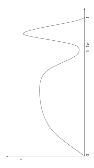
Figure 1. Schematic picture of $p_{n}$. On the right the wave is a high peak with length of order $1/n$ and height of order $n$. By contrast, the bulk has height and length of order one.

Theorem 1.

Suppose that the fitness distribution $q$ satisfies

$$\lim_{h\downarrow 0}\frac{q(1-h,1)}{h^{\alpha}}=1,$$ (1.2)

where $\alpha>1$, and that (1.1) holds. Then, for $x>0$,

$$\lim_{n\uparrow\infty}p_{n}(1-\frac{x}{n},1)=\frac{\gamma(\beta)}{\Gamma(\alpha)}\int_{0}^{x}y^{\alpha-1}e^{-y}\,dy.$$ (1.3)

We remark that the total mass in the ‘wave’ moving towards the maximal fitness value agrees with the mass of the atom in the limiting distribution $p(dx)$. Its rescaled shape is that of a gamma distribution with shape parameter $\alpha$.

2. Proof of Theorem 1

Note that

$$\mu_{n}=\int x^{n}\,q(dx)\sim\Gamma(\alpha+1)\,n^{-\alpha},$$

where the asymptotics is easily derived from (1.2), and note that

$$\sum_{n=0}^{\infty}\mu_{n}=\int_{0}^{1}\frac{q(dx)}{1-x}=\frac{1}{\beta}\,(1-\gamma(\beta)).$$ (2.1)

Also define

$$W_{n}:=w_{1}\cdots w_{n}.$$

Given the family $(W_{n})_{n\geq 1}$ the fitness distributions can be obtained as

$$p_{n}(dx)=\sum_{r=0}^{n-1}\frac{W_{n-r}}{W_{n}}\,(1-\beta)^{r}\beta\,x^{r}\,q(dx)+\frac{1}{W_{n}}\,(1-\beta)^{n}\,x^{n}\,p_{0}(dx),$$ (2.2)

see [9, (2.1)]. The main tool in the proof is therefore the following lemma.

Lemma 2.

We have, as $n\uparrow\infty$,

$$W_{n}\sim c\,n^{-\alpha}(1-\beta)^{n-1},$$

where

$$c=\frac{\beta}{\gamma(\beta)}\,\Gamma(\alpha+1)\,\sum_{k=1}^{\infty}W_{k}\,(1-\beta)^{1-k}.$$

Proof.

Integrating (2.2) we obtain [9, (2.3)]

$$W_{n}=\sum_{r=1}^{n-1}W_{n-r}\,(1-\beta)^{r-1}\beta\,\mu_{r}+(1-\beta)^{n-1}\,m_{n}.$$

Abbreviate $u_{n}:=W_{n}\,(1-\beta)^{1-n}.$ Then $u_{n}$ satisfies the renewal equation

$$u_{n}=\mbox{$\frac{\beta}{1-\beta}$}\,\sum_{r=1}^{n-1}u_{n-r}\mu_{r}+m_{n},\qquad\mbox{ for }n\geq 1.$$

Using (2.1), we obtain $\frac{\beta}{1-\beta}\sum_{n=1}^{\infty}\mu_{n}=1-\frac{\gamma(\beta)}{1-\beta}<1$. Hence, the renewal theorem, see e.g. [8, XXXIII.10, Theorem 1], implies that

$$\sum_{n=1}^{\infty}u_{n}=\frac{\sum_{n=1}^{\infty}m_{n}}{1-\frac{\beta}{1-\beta}\,\sum_{n=1}^{\infty}\mu_{n}}=\frac{1-\beta}{\gamma(\beta)}\sum_{n=1}^{\infty}m_{n}<\infty$$

where the finiteness follows since $m_{n}$ is bounded by a constant multiple of $\mu_{n}$ and

$$\sum_{n=0}^{\infty}\mu_{n}=\int\frac{q(dx)}{1-x}<\infty.$$

Fix $\delta>0$ and $0<\varepsilon<\eta<1$ and suppose $n$ is large enough such that $\eta n\leq n-1$ and

$$\mu_{r}\leq(\Gamma(\alpha+1)+\delta)\,r^{-\alpha}\quad\mbox{ for all }r\geq(1-\eta)n.$$

For an inductive argument suppose that $c_{1},\ldots,c_{r}$ are chosen such that $u_{r}\leq c_{r}\,r^{-\alpha}$ for all $\varepsilon n\leq r\leq n-1$. Then one has for $r=1,\dots,n-1$

$$u_{r}\mu_{n-r}\leq\begin{cases}(1-\varepsilon)^{-\alpha}(\Gamma(\alpha+1)+\delta)n^{-\alpha}u_{r}&\text{ if }r\leq\varepsilon n,\\ c_{r}\,(\Gamma(\alpha+1)+\delta)r^{-\alpha}(n-r)^{-\alpha}&\text{ if }\varepsilon n\leq r\leq\eta n,\\ c_{r}\,\eta^{-\alpha}n^{-\alpha}\mu_{n-r}&\text{ if }\eta n\leq r,\end{cases}$$

so that

$$u_{n} \leq(1-\varepsilon)^{-\alpha}\,\mbox{$\frac{\beta}{1-\beta}$}\,(\Gamma(\alpha+1)+\delta)\,\Bigl{(}\sum_{r=1}^{\infty}u_{r}\Bigr{)}\,n^{-\alpha}\,$$

$$\phantom{space}+\mbox{$\frac{\beta}{1-\beta}$}\,(\Gamma(\alpha+1)+\delta)\,\Bigl{(}\mbox{$\frac{1}{n}$}\sum_{r=\lfloor\varepsilon n\rfloor+1}^{\lfloor\eta n\rfloor}c_{r}\,\bigl{(}\mbox{$\frac{r}{n}$}\bigr{)}^{-\alpha}\bigl{(}1-\mbox{$\frac{r}{n}$}\bigr{)}^{-\alpha}\Bigr{)}n^{1-2\alpha}\,$$ (2.3)

$$\phantom{space}+\mbox{$\frac{\beta}{1-\beta}$}\,\eta^{-\alpha}\,\Bigl{(}\sum_{r=\lfloor\eta n\rfloor+1}^{n-1}c_{r}\,\mu_{n-r}\Bigr{)}n^{-\alpha}+m_{n}=:c_{n}n^{-\alpha}.$$

By induction this yields a sequence $(c_{n})$ with $u_{n}\leq c_{n}\,n^{-\alpha}$ for all $n\geq 1$.

Using that $m_{n}n^{\alpha}\to 0$ by assumption, and that the term (2.3) is bounded by a constant multiple of

$$n^{1-2\alpha}\,\int_{\varepsilon}^{\eta}dr\,r^{-\alpha}(1-r)^{-\alpha}\ll n^{-\alpha},$$

we see that $(c_{n})$ converges to the unique solution $c^{*}=c^{*}(\varepsilon,\delta,\eta)$ of

$$c^{*}=(1-\varepsilon)^{-\alpha}\,\mbox{$\frac{\beta}{1-\beta}$}\,(\Gamma(\alpha+1)+\delta)\,\sum_{r=1}^{\infty}u_{r}+c^{*}\,\eta^{-\alpha}\,\mbox{$\frac{\beta}{1-\beta}$}\,\sum_{r=1}^{\infty}\mu_{r}.$$

Recalling that $\beta\sum_{r=1}^{\infty}\mu_{r}=1-\gamma(\beta)-\beta$, and letting $\varepsilon,\delta\downarrow 0$ and $\eta\uparrow 1$ we see that $c^{*}(\varepsilon,\delta,\eta)$ converges to

$$c=\frac{\beta}{\gamma(\beta)}\,\Gamma(\alpha+1)\,\sum_{k=1}^{\infty}u_{k}=\frac{\beta}{\gamma(\beta)}\,\Gamma(\alpha+1)\,\sum_{k=1}^{\infty}W_{k}\,(1-\beta)^{1-k},$$

which yields the upper bound. The lower bound can be derived similarly. ∎

To complete the proof using the lemma, we look at (2.2) and get

$$p_{n}\big{(}1-\frac{x}{n},1\big{)} =\sum_{r=0}^{n-1}\frac{W_{n-r}}{W_{n}}\,(1-\beta)^{r}\beta\,\int_{1-x/n}^{1}y^{r}\,q(dy)+\frac{1}{W_{n}}\,(1-\beta)^{n}\,\int_{1-x/n}^{1}y^{n}\,p_{0}(dy).$$

The second term vanishes asymptotically, as

$$\frac{1}{W_{n}}\,(1-\beta)^{n}\,\int_{1-x/n}^{1}y^{n}\,p_{0}(dy)\sim(1-\beta)\,\frac{m_{n}}{cn^{-\alpha}}\frac{\int_{1-x/n}^{1}y^{n}\,p_{0}(dy)}{\int_{0}^{1}y^{n}\,p_{0}(dy)}\to 0,$$

using our assumption that $m_{n}/\mu_{n}\to 0$. The first term is asymptotically equivalent to

$$n^{\alpha}\sum_{r=0}^{n-1}W_{n-r}\,c^{-1}\,(1-\beta)^{1-n+r}\beta\,\int_{1-x/n}^{1}y^{r}\,q(dy).$$

By chosing a large $M$, the contribution coming from terms with $r\leq n-Mn^{1/\alpha}$ can be bounded by a constant multiple of

$$(n-Mn^{1/\alpha})\,\Big{(}\frac{n}{Mn^{1/\alpha}}\Big{)}^{\alpha}q\big{(}1-\mbox{$\frac{x}{n}$},1\big{)},$$

which is bounded by an arbitraily small constant. For the remaining terms we can now use that

$$\int_{1-x/n}^{1}y^{sn}\,q(dy) \sim\int_{x}^{0}e^{-as}\,dq(1-\mbox{$\frac{a}{n}$},1)\sim\alpha\,n^{-\alpha}\int_{0}^{x}a^{\alpha-1}e^{-as}\,da,$$

and a change of variables to obtain equivalence to

$$\alpha\,\beta\,c^{-1}\Big{(}\sum_{m=1}^{\infty}W_{m}\,(1-\beta)^{1-m}\Big{)}\,\int_{0}^{x}a^{\alpha-1}e^{-a}\,da,$$

and the result follows as, by Lemma 2,

$$\alpha\,\beta\,c^{-1}\Big{(}\sum_{m=1}^{\infty}W_{m}\,(1-\beta)^{1-m}\Big{)}=\frac{\gamma(\beta)}{\Gamma(\alpha)},$$

as required.

3. Discussion

Kingman’s model is on the one hand one of the simplest models in which a condensation effect can be observed, on the other hand it is sufficiently rich to study the emergence of condensation as a dynamical phenomenon. The simplicity of the model allows a rigorous treatment with elementary means, but we believe that our calculation has far reaching consequences as a variety of much more complex models in quite diverse areas of science have similar features. Among the models we expect to share many features with Kingman’s model are models of the physical phenomenon of Bose-Einstein condensation, of wealth condensation in macroeconomics, or the emergence of traffic jams.

Our main conjecture is that in a large universality class of models in which effects similar to mutation and selection compete effectively on a bounded and continuous statespace, the ‘wave’ moving towards the maximal state forming the condensate is of a Gamma shape.

Random models which are suitable test cases for our universality claim arise, for example, in the study of random permutations with cycle weights. Here the probability of a permutation $\sigma$ in the symmetric group on $n$ elements is defined as

$$\mathbb{P}_{n}(\sigma)=\frac{1}{n!h_{n}}\prod_{j\geq 1}\theta_{j}^{R_{j}(\sigma)},$$

where $R_{j}(\sigma)$ is the number of cycles of length $j$ in $\sigma$ and $h_{n}$ is a normalisation constant. For our investigation we focus on the case that $\theta_{j}\sim j^{\gamma}$ for $\gamma\in\mathbb{R}$. We now discuss results of Betz, Ueltschi and Velenik [3] and Ercolani and Ueltschi [7] in our context.

Our interest is in the empirical cycle length distribution which is the random measure on $[0,1]$ given by

$$\mu_{n}=\frac{1}{n}\sum_{i=1}^{n}\lambda_{i}\,\delta_{\frac{\lambda_{i}}{n}},$$

where the integers $\lambda_{1}\geq\lambda_{2}\geq\cdots$ are the ordered cycle lengths of a permutation chosen randomly according to $\mathbb{P}_{n}$. The asymptotic behaviour of $\mu_{n}$ shows three phases depending on the value of the parameter $\gamma$, see Table 1 in [7]:

• If $\gamma<0$ large cycles are preferred and the empirical cycle length distribution concentrates asymptotically in the point $1$,

• if $\gamma=0$ there is no condensation and we have convergence to a beta distribution,

• if $\gamma>0$ we see a preference for short cycles and the empirical cycle length distribution concentrates asymptotically in the point $0$.

In the two phases in which see a condensation effect we have partial information on the shape of the wave, which is consistent with our universality claim.

Let us first look at the case $\gamma>0$ when the empirical cycle length distribution concentrates in the left endpoint of our domain, i.e. the normalised cycle lengths vanish asymptotically. In this case Theorem 5.1 of [7] shows that, for $\alpha=\frac{\gamma}{\gamma+1}$,

$$\lim_{n\to\infty}\mathbb{E}\big{[}\mu_{n}[0,\mbox{$\frac{x}{n^{\alpha}}$})\big{]}=\frac{1}{\Gamma(\gamma+1)}\,\int_{0}^{x}y^{\gamma}e^{-y}\,dy,$$

i.e. focusing on the left edge of the domain in the scale $1/n^{\alpha}$ we see a gamma distributed wave shape with parameter $\gamma$, at least in the mean. It is a natural conjecture that this convergence holds not only in expectation, but also in probability, and establishing this fact is subject of an ongoing project.

If $\gamma<0$ large cycles are preferred. Here the situation is slightly different because the wave sweeping towards the maximal normalised cyclelength is on the critical scale $1/n$ and this means that we expect that the discrete nature of $\mu_{n}$ is retained in the limit.

More precisely, Theorem 3.2 of [3] implies that

$$\lim_{n\to\infty}\mathbb{E}\big{[}\mu_{n}[1-\mbox{$\frac{m}{n}$},1]\big{]}=\mbox{$\frac{1}{2}$}\,\sum_{n=0}^{m}e^{-c^{*}n}h_{n},$$

where $c^{*}$ is a ‘Malthusian parameter’ chosen such that

$$\sum_{n=1}^{\infty}e^{-c^{*}n}h_{n}=1.$$

We further note that $h_{n}\sim C\,n^{\gamma-1}$ by [7, (7.1)] and so we are still able to recognise a discrete form of a gamma distribution with parameter $\gamma$ in this case.

The most elaborate model in which we were able to test our hypothesis is a random network model with fitness. We now give an informal preview of forthcoming results of Dereich [5], which are motivated by a problem of Borgs et al.  [4].

A preferential attachment network model is a sequence of random graphs $(\mathcal{G}(n))_{n\in\mathbb{N}}$ that is built dynamically: one starts with a graph $\mathcal{G}(1)$ consisting of a single vertex $1$ and, in general, the graph $\mathcal{G}({n+1})$ is built by adding the vertex $n+1$ to the graph $\mathcal{G}(n)$ and by insertion of edges connecting the new vertex to the graph $\mathcal{G}(n)$ according to an attachment rule. Typically, the attachment rule rewards vertices that already have a high degre: in most cases the degree of a vertex has an affine influence on its attractiveness in the collection of new edges. In a preferential attachment model with fitness one additionally assigns each vertex an intrinsic fitness, a positive number, which has a linear impact on its attractiveness in the network formation.

Let us be more precise about the variant of the network model to be considered in the rest of this paper. We consider a sequence of random directed graphs $(\mathcal{G}(n))_{n\in\mathbb{N}}$ and denote by

$$\mathrm{imp}_{n}(m):=\mathrm{indegree}_{\mathcal{G}(n)}(m)+1$$

the impact of the vertex $m\in\{1,\dots,n\}$ in $\mathcal{G}(n)$. Further, let $F_{1},F_{2},\dots$ denote a sequence of independent $q$-distributed random variables modeling the fitness of the individual vertices $1,2,\ldots$. The attachment rule is as follows: given the graph $\mathcal{G}(n)$ and all fitnesses, link $n+1$ to each individual vertex $m\in\{1,\dots,n\}$ with an independent Poisson distributed number of edges with parameter

$$\frac{1}{n\,Z_{n}}\,{F_{m}\,\mathrm{imp}_{n}}(m),$$

where $Z_{n}$ is a normalisation which depends only on $\mathcal{G}(n)$ and the fitnesses. Note that all links point from new to old vertices so that orientations can be recovered from the undirected set of edges. We consider two types of normalisations:

1. adaptive normalisation: $Z_{n}=\frac{1}{\lambda n}\sum_{m=1}^{n}F_{m}\,\mathrm{imp}_{n}(m)$ for a parameter $\lambda>0$,
   

2. deterministic normalisation: $(Z_{n})$ is a deterministic sequence.

In the case of adaptive normalisation, the outdegree of $n+1$ is Poisson distributed with parameter $\lambda$, even when conditioning on the graph $\mathcal{G}(n)$. Hence, the total number of edges is almost surely of order $\lambda n$ so that $\frac{1}{n}\sum_{m=1}^{n}\mathrm{imp}_{n}(m)$ converges almost surely to $\lambda+1$.

The analogue of $p_{n}$ is the impact measure given by

$$\Xi_{n}=\frac{1}{n}\sum_{m=1}^{n}\mathrm{imp}_{n}(m)\,\delta_{F_{m}}.$$

It measures the contribution of the vertices of a particular fitness to the total impact.

As observed in [1] and verified for a different variant of the model in [4], network models with fitness show a phase transition similar to Bose-Einstein condensation. The verification of this phase transition in the variant considered here is conducted in [6].

For adaptive normalisation two regimes can be observed

1. $\int\frac{1}{1-x}\,q(dx)\geq 1+\lambda$: the fit-get-richer phase,
   

2. $\int\frac{1}{1-x}\,q(dx)<1+\lambda$: the Bose-Einstein phase or innovation-pays-off phase.

In the fit-get-richer phase, the random measures $(\Xi_{n})_{n\in\mathbb{N}}$ converge almost surely in the weak topology to the measure $\Xi$ on $(0,1]$ given by

$$\Xi(dx)=\frac{\lambda^{*}}{\lambda^{*}-x}\,q(dx),$$

where $\lambda^{*}\in[1,\infty)$ denotes the unique solution to

$$\int\frac{\lambda^{*}}{\lambda^{*}-x}\,q(dx)=1+\lambda,$$

whereas, in the Bose-Einstein phase, one observes convergence to

$$\Xi(dx)=\frac{1}{1-x}\,q(dx)+\Bigl{(}1+\lambda-\int\frac{1}{1-y}\,q(dy)\Bigr{)}\delta_{1}(dx).$$

In order to analyse the emergence of the condensation phenomenon, we consider the preferential attachment model with deterministic normalisation. We assume that $q$ is regularly varying at $1$ with representation

$$q(1-h,1)=h^{\alpha}\,\ell(h),$$

where $\ell:[0,1]\to(0,\infty)$ is a slowly varying function. In order to replicate the Bose-Einstein phenomenon in the model with deterministic normalisation, one needs to choose $(Z_{n})$ appropriately. For $1\leq m\leq n$, let

$$\Upsilon[m,n]:=\sum_{k=\lfloor m\rfloor}^{\lfloor n\rfloor}\frac{1-Z_{k}}{k}.$$

The Bose-Einstein phenomenon can be replicated by choosing $(Z_{n})$ such that

$$1-Z_{n}\sim\alpha(\log n)^{-1}$$

and such that the limit

$$\gamma:=\lim_{n\to\infty}\frac{\alpha}{\alpha-1}\Gamma(\alpha)\,\frac{(\log n)^{\alpha}\cdot\log(\log n)^{\alpha}}{\ell((\log n)^{-1})}\,\exp\{\Upsilon[\log n,n]\}$$ (3.1)

exists. We stress that such a normalisation can be found for various fitness distributions $q$ and we refer the reader to the article [5] for the details.

Theorem 3.

Under the above assumptions, one has, for $x>0$,

$$\lim_{n\to\infty}\Xi_{n}\Bigl{(}1-\frac{x}{\log n},1\Bigr{)}=\frac{\gamma}{\Gamma(\alpha)}\int_{0}^{x}y^{\alpha-1}e^{-y}\,dy,\text{ in probability}.$$

For any measurable set $A\subset[0,1]$ with $1\not\in\partial A$, one has

$$\lim_{n\to\infty}\Xi_{n}(A)=\Xi(A),\text{ in probability},$$

for the measure $\Xi$ on $[0,1]$ given by

$$\Xi(dx)=\frac{1}{1-x}\,q(dx)+\gamma\,\delta_{1}(dx).$$

Remark 1.

In most cases one cannot give an explicit representation for a normalisation $(Z_{n})$ satisfying (3.1). On first sight, this might be suprising since the $(Z_{n})$ play a rôle analogous to $(W_{n})$ in the Kingman model where the analysis is feasible. The difference of both models comes from the stochastic nature of the network model. In order to analyse the network model one could start to work with expectations resulting in a mean field model similar to the Kingman model. However, the expectations for $\Xi_{n}$ are dominated by configurations that are not seen in typical realisations: vertices of particular high fitness that are born very early contribute most although being not present typically. To compensate this the normalisations in the network model have to be slightly smaller than a mean field model would suggest. Vertices of particularly high fitness have an impact only with a delay. This causes the $\Upsilon[\log n,n]$ term in (3.1) and makes explicit representations for $(Z_{n})$ in many cases unfeasible.

We conclude our discussion with the remark that the case of unbounded fitness distribution is also of considerable interest. In this case Park and Krug [10] have studied the analogue of Kingman’s model and (in a particular case) observed emergence of a travelling wave of Gaussian shape. They also conjecture that this behaviour is of universal nature.

Acknowledgments: The second author acknowledges useful discussions with Daniel Ueltschi at the Oberwolfach workshop Interplay of analysis and probability in physics, January 2012. We would like to thank Marcel Ortgiese for agreeing to include a preview of [6] in our discussion.

References

- [1] Bianconi, G. and Barabási, A.-L. (2001) Bose-Einstein condensation in complex networks. Phys. Rev. Lett. 86, 5632–35.
- [2] Bianconi, G.,Ferretti, L. and Franz, S. (2009) Non-neutral theory of biodiversity. Europhys. Lett. 87, P07028.
- [3] Betz, V., Ueltschi, D. and Velenik, Y. (2011) Random permutations with cycle weights. Ann. Appl. Probab. 21, 312–331.
- [4] Borgs, C., Chayes, J.T., Daskalakis, C. and Roch, S. (2007) First to market is not everything: an analysis of preferential attachment with fitness. In: STOC ’07 Proceedings of the thirty-ninth annual ACM symposium on theory of computing. pp. 135–144.
- [5] Dereich, S. (2012) In Preparation.
- [6] Dereich, S. and Ortgiese, M. (2012) In Preparation.
- [7] Ercolani, N.M. and Ueltschi, D. (2011) Cycle strucure of random permutations with cycle weights. Preprint arxiv:1102.4796.
- [8] Feller, W. (1968) An introduction to probability theory and its applications. Vol. I. Third edition, Wiley.
- [9] Kingman, J.F.C. (1978) A simple model for the balance between selection and mutation. J. Appl. Prob. 15, 1–12.
- [10] Park, S.-C. and Krug, J. (2008) Evolution in random fitness landscapes: the infinite sites model. J. Stat. Mech. Theory Exp. no. 4, P04014, 29pp.