Abstract

We consider a hydrodynamic-type system of balance equations for mass and momentum closed by the dynamical equation of state taking into account the effects of spatial nonlocality. We study higher symmetries and local conservation laws for this system and establish its nonintegrability for the generic values of parameters. A system of ODEs obtained from the system under study through the group theory reduction is investigated. The reduced system is shown to possess a family of the homoclinic solutions describing solitary waves of compression and rarefaction. The waves of compression are shown to be unstable. On the contrary, the waves of rarefaction are likely to be stable. Numerical simulations reveal some peculiarities of solitary waves of rarefaction, and, in particular, the recovery of their shape after the collisions

Keywords nonlocal hydrodynamic-type model; integrability tests; spectral stability of soliton-like solutions; interaction of solitary waves

1 Introduction

This paper deals with soliton-like traveling wave (TW) solutions to some nonlinear evolutionary PDEs. The TW solutions play an important role in mathematical physics. They appear in the models of various transport phenomena, including the shallow water equation [1], the lithosphere model [2], the nerve axon model [3, 4, 5], models of combustion theory [6], mathematical biology [7], and active dissipative media models [8, 9] (for further examples see [10, 11] and references therein). Among the great variety of nonlinear wave solutions, perhaps the most important are solitons, supported, in particular, by the celebrated Korteweg–de Vries (KdV) equation. After the the discovery of integrability of the KdV equation in the second half of the XX-th century, the study of solitons attracted attention of a great many authors, see e.g. [1] and references therein. The unusual features of soliton solutions, in particular their particle-like collisions and the existence of a broad set of smooth Cauchy data asymptotically turning into a finite number of solitons in the course of time evolution, have usually been attributed to the complete integrability of the KdV equation, and certain attendant properties, such as the infinite symmetry and existence of an infinite number of local conservation laws [38, 39]. Later on it was observed that solutions to the equations which are not completely integrable manifest features similar to those demonstrated by ”true” solitons. A prominent example of this is provided by the so-called compactons, supported by the equations of the $K(m,n)$ family, introduced by J. Hyman and Ph. Rosenau in 1993 [16]. The non-integrability of a generic member of the class of Hyman–Rosenau $K(m,n)$ equations stems inter alia from the fact that only a finite number of higher symmetries is known and only four local conservation laws have been obtained to date [17] (it was rigorously proved recently that the $K(m,n)$ equations for $m=n$ and $m\neq-2,-1/2,0,1$ have just four conservation laws and no higher symmetries [18]). The family of non-integrable evolutionary equations possessing stable localized solutions with soliton features is not exhausted by the generic $K(m,n)$ equations. Other non-integrable models with similar features of soliton-like solutions are presented in [19, 20, 21, 22, 23, 24, 25].

The main goal of the present paper is to demonstrate the existence of stable soliton-like TW solutions in a hydrodynamic-type model taking into account the effects of spatial nonlocality. The study of higher symmetries and local conservation laws admitted by the system under study reveals its non-integrability for generic values of parameters. Nevertheless, the solitary waves supported by this system restore their shapes after the mutual collisions. Furthermore, a proper choice of the Cauchy data leads to the creation of a chain of solitary waves moving with distinct velocities.

The paper is organized as follows. In section 2 we introduce our basic system of PDEs and study its higher symmetries and local conservation laws. Using these results, we establish non-integrability of this system for generic values of parameters. In section 3 we give a geometric insight into the structure of the phase space of the dynamic system obtained through the symmetry-based reduction of the initial system, and formulate the conditions which guarantee that the reduced system possesses a one-parameter family of homoclinic solutions corresponding to the solitary wave regimes. In section 4 we study the perturbed solitary wave solutions and estimate the essential spectrum of the linearized problem. In section 5 we perform a numerical study of stability for the solitary waves of rarefaction (dark solitons) using the Evans function and investigate some peculiarities of the solitary waves, such as the dependence of their maximal depth and the effective width on the wave velocity, evolution of the initial non-solitonic perturbation and the behavior of waves in the course of their collisions. Finally, in section 6 we discuss the results obtained and give an outline of further research.

2 The model system and its symmetry properties

It is well known that the features of TW depend in essence on dispersive and nonlinear properties of physical media [12, 13, 1, 26, 27, 28, 29]. Let us stress that in many cases nonlocal effects caused by internal structure of the media can also play significant role in formation and evolution of wave patterns. The presence of internal structure causes various effects such as the fragmentation of smooth initial perturbations and intensification of shock fronts in the models of heterogeneous media [8, 14], soliton and compacton features of the block media models [1, 22, 16], and many others.

Unfortunately, there exists no universal model describing structured media in a sufficiently wide range of the values of parameters. Below we introduce a model system taking into account the nonlocal effects related to the presence of internal structure (cf. [30, 31, 32]). This model applies when the ratio of the characteristic size $d$ of elements of the structure to the characteristic wavelength $\lambda$ of the wave pack is much smaller than unity and therefore the continual approach is still valid but the said ratio is not small enough to ignore the presence of internal structure. As it is shown in [33, 34], the balance equations for mass and momentum of media with internal structure in the long-wave approximation still retain their classical form, which in the one-dimensional case reads

$$\left\{\begin{array}[]{ll}u_{t}+p_{x}=0,\\ \rho_{t}+\rho^{2}u_{x}=0.\end{array}\right.$$ (1)

Here $u$ denotes the mass velocity, $p$ is the pressure, $\rho$ is the density, t is the time, $x$ is the mass (Lagrangian) coordinate related to the conventional spatial coordinate $x_{e}$ as follows:

$$x=\int^{x_{e}}{\rho(t,\,\xi)\,d\,\xi}.$$

The subscripts $t$ and $x$ denote partial derivatives with respect to indicated variables.

Thus, the entire information about the presence of structure in this approximation is contained in a dynamical equation of state (DES) which should be incorporated into the system (1) in order to make it closed. In general, DES for structured media manifesting the nonlocal features takes the form of an integral equation [35, 36] relating the generalized thermodynamical flow $J$ and the generalized thermodynamical force $X$ causing this flow:

$$J=\int_{-\infty}^{t}\left[\int_{R}K(t,t^{\prime};\,x,x^{\prime})X(t^{\prime},x^{\prime})\,dx^{\prime}\right]\,dt^{\prime}.$$ (2)

Here $K(t,t^{\prime};\,x,x^{\prime})$ is the kernel of nonlocality. The function $K$ can be calculated by solving the dynamical problem of structure elements interaction; however, such calculations are extremely difficult. Therefore, in practice one uses, as a rule, some model kernel describing well enough the main properties of the nonlocal effects and, in particular, the fact that these effects vanish rapidly as $|t-t^{\prime}|$ and $|x-x^{\prime}|$ grow. This property could be used for passing from the integral equation (2) to a purely differential equation.

One of the simplest equations of state taking into account the effects of spatial nonlocality takes the form

$$p=\hat{\sigma}\,\int_{-\infty}^{+\infty}K_{1}\left(x,\,x^{\prime}\right)\,\rho^{n}(t,\,x^{\prime})\,dx^{\prime},$$ (3)

where $K_{1}\left(x,\,x^{\prime}\right)=\exp\left[-{(x-x^{\prime})^{2}}/{l^{2}}\right]$ is the kernel accounting for a purely spatial nonlocality. This model is attributed in [30] to the situation when the density of a medium changes abruptly from point to point, as this is the case with an elastic body containing the microcracks or low density solid inclusions.

Using the fact that the function $\exp{\left[-(x-x^{\prime})^{2}/{l^{2}}\right]}$ extremely quickly approaches zero as $|x-x^{\prime}|$ grows, one can replace the function $\rho^{n}(t,\,x^{\prime})$ by several terms of its power series expansion,

$$\rho^{n}(t,\,x^{\prime})=\rho^{n}(t,\,x)+[\rho^{n}(t,\,x)]_{x}\frac{x^{\prime}-x}{1!}+[\rho^{n}(t,\,x)]_{xx}\frac{\left(x^{\prime}-x\right)^{2}}{2!}+O(|x-x^{\prime}|^{3}),$$

obtaining in this way the following approximate flow-force relation:

$$p=c_{0}\,\rho^{n}(t,\,x)+c_{2}\,\left[\rho^{n}(t,x)\right]_{xx}.$$ (4)

Here

$$c_{0}=\hat{\sigma}\,l\int_{-\infty}^{+\infty}e^{-\tau^{2}}d\tau=\hat{\sigma}\,l\sqrt{\pi},\qquad c_{2}=\hat{\sigma}\,\frac{l^{3}}{2}\int_{-\infty}^{+\infty}\tau^{2}e^{-\tau^{2}}d\tau=\hat{\sigma}\,\frac{l^{3}\,\sqrt{\pi}}{4}.$$

so both of the coefficients are positive. Choosing the kernel in the form

$$K(x^{\prime},\,x)=\hat{\sigma}\,\left[\mu+\alpha\,(x-x^{\prime})^{2}\right]\,\exp\left[-{(x-x^{\prime})^{2}}/{l^{2}}\right]$$

and following the procedure outlined above, we obtain the dynamical equation of state

$$p=\hat{\sigma}\,\sqrt{\pi}\,\left\{\rho^{n}(t,\,x)\,l\,\left(\mu+\frac{\alpha}{2}\,l^{2}\right)+\,\left[\rho^{n}(t,x)\right]_{xx}l^{3}\,\left(\frac{\mu}{4}+\frac{3}{8}\alpha\,l^{2}\right)\right\}=$$

$$=\tilde{c_{0}}\,\rho^{n}(t^{\prime},x)+\tilde{c_{2}}\,\left[\rho^{n}(t,x)\right]_{xx}.$$

For $\alpha=-1,\qquad{l^{2}}/{2}<\mu<{3\,l^{2}}/{2}$ $\tilde{c_{0}}$ remains positive while $\tilde{c_{2}}$ becomes negative. Note that a well-established linear strain-stress dependence corresponding to the above situation is presented in [37]. Nonlinear strain-stress relationship of this type can be used for the description of wave movements in the pre-stressed structured medium [22].

Thus, we consider the model system

$$\left\{\begin{array}[]{l}u_{t}+\beta\rho^{\nu+1}\rho_{x}+\gamma\left[\rho^{\nu+1}\rho_{xxx}+3(1+\nu)\rho^{\nu}\rho_{x}\rho_{xx}+\nu(1+\nu)\rho^{\nu-1}\rho^{3}_{x}\right]=0,\\ \\ \rho_{t}+\rho^{2}u_{x}=0,\end{array}\right.$$ (5)

assuming that $\beta>0$ and $\gamma\neq 0$.

Let us turn to the study of integrability properties of (5). We shall use the integrability test based on existence of higher symmetries, see e.g. [41, 42] for details, because it allows to detect both integrability via the inverse scatttering transform and linearizability through a suitably chosen transformation and, unlike, say, the search for a Lax representation, verifying the existence of higher symmetries is an algorithmic procedure.

First of all, note that for $\nu=-3$ the change of variables $u=u$, $r=1/\rho$ linearizes this system into

$$\begin{array}[]{ll}u_{t}+\beta r_{x}+\gamma r_{xxx}=0,\\ r_{t}-u_{x}=0,\end{array}$$ (6)

so for $\nu=-3$ the system (5) is integrable (more precisely, in this case it is $C$-integrable, i.e., linearizable).

Now turn to the case $\nu\neq-3$ and perform the following change of variables: $v=\rho$, $w=u+c\rho^{(\nu-1)/2}\rho_{x}$, where $c=\sqrt{\gamma}$. It converts our system into the following

$$\begin{array}[]{ll}v_{t}=-cv^{(\nu+3)/2}v_{xx}-(c/2)v^{(\nu-1)/2}(\nu-1)v_{x}^{2}-v^{2}w_{x},\\ w_{t}=cv^{(\nu+3)/2}u_{xx}-(\nu+3)(c^{2}/2)(v^{\nu}v_{x}^{2})_{x}+c(\nu+3)v^{(\nu+1)/2}u_{x}v_{x}/2-bv^{\nu+1}v_{x}.\end{array}$$ (7)

The matrix at the second derivatives in (7) has the form

$$A=\left(\begin{array}[]{rl}-cv^{(\nu+3)/2}&0\\ -c^{2}(\nu+3)v^{\nu}v_{x}&cv^{(\nu+3)/2}\end{array}\right)$$ (8)

with two distinct eigenvalues $\pm\lambda$, where $\lambda=cv^{(\nu+3)/2}$.

Then a necessary condition for (7) to admit local higher, also known as generalized [38], symmetries (see e.g. [40, 38, 39] and references therein for details) of order greater than two is (see e.g. [42]) that the quantity $\lambda^{-1/2}$ is a (local) conserved density for (7), i.e., there exists a $\sigma$ depending on $x,t,v,w$ and a finite number of $x$-derivatives of $v$ and $w$ such that $D_{t}(\lambda^{-1/2})=D_{x}(\sigma)$ by virtue of (7). However, it is readily checked that $\lambda^{-1/2}$ is a conserved density for (7) only if $\nu=-3$ or $\nu=1$. Therefore, for $\nu\neq-3,1$ the system (7) has local higher symmetries of order at most two. These are easily seen to have been exhausted by the Lie point symmetries (more precisely, by symmetries equivalent to the Lie point ones).

Going back to (5) and making use of the transformation properties of higher symmetries, see e.g. [40, 39], we conclude that (5) has no symmetries of order greater than three. The computation of symmetries of order not greater than three shows that for $\nu\neq-3,1$ the only local higher symmetries of (7) are (equivalent to) the Lie point ones:

$$\begin{split}Q_{1}&=\partial/\partial u,\\ Q_{2}&=\partial/\partial x,\\ Q_{3}&=\partial/\partial t,\\ Q_{4}&=(\nu+3)t\partial/\partial t-(\nu+1)u\partial/\partial u-2\rho\partial/\partial\rho.\\ \end{split}$$ (9)

Thus, for $\nu\neq-3,1$ the system (5) is non-integrable, at least in the sense of absence of genuinely higher symmetries, which is a strong indicator of non-integrability in any other sense as well, cf. [41, 42, 38].

The Lie point symmetries (9) have a clear physical interpretation: the first three are translations w.r.t. independent variables and the dependent variable $u$ while the last one is the scaling symmetry. Somewhat surprisingly, this scaling symmetry does not involve $x$.

For the generic values of parameters these are the only (be it Lie point or higher) symmetries admitted by the system (5). However, for special values of parameters additional symmetries may emerge.

For instance, if we concentrate on the physically relevant case of $\nu\,\geq\,0$, we easily find that for $\nu=1$ there appears an additional nonlocal symmetry. Namely, consider the extended (also known as potential, see e.g. [39] for details) system which consists of (5) and the equations for the potential $q$ of the conservation law given by the second equation of (5), that is,

$$q_{x}=1/\rho,\quad q_{t}=u.$$ (10)

The said extended system for $\nu=1$ possesses the following additional symmetry:

$$Q_{5}=-t^{2}\partial/\partial t+(tu-q)\partial/\partial u+t\rho\partial/\partial\rho+(t^{2}u-tq)\partial/\partial q.$$

In spite of the presence of this additional nonlocal symmetry it is rather unlikely that the case of $\nu=1$ is integrable but the definitive settling of this issue requires further research.

Recall now that a local conservation law for the system (5) is a relation of the form

$$D_{t}R-D_{x}S,$$

vanishing modulo (5) and its differential consequences, where $R,\,S$ depend on $x,t,u,\rho$ and a finite number of $x$-derivatives of $u$ and $\rho$, $D_{t}$ and $D_{x}$ denote the total derivative w.r.t. the temporal and spatial variables, respectively, cf. [40, 38, 39] for details.

The local conservation laws associated with (5) read as follows:

$$R_{1} =u,\quad S_{1} =-\frac{\beta}{\nu+2}\rho^{\nu+2}-\gamma\left(\rho^{\nu+1}\rho_{x}\right)_{x}$$ (11)

$$R_{2} =1/\rho,\quad S_{2} =u,$$

$$R_{3} =u\,\sin(\omega\,x),\quad S_{3} =\frac{\cos(\omega\,x)}{\omega}\,\beta\rho^{\nu+1}\rho_{x}-\sin(\omega x)\gamma\left(\rho^{\nu+1}\rho_{x}\right)_{x},$$

$$R_{4} =u\,\cos(\omega x),\quad S_{4} =-\frac{\sin(\omega x)}{\omega}\beta\rho^{\nu+1}\rho_{x}-\cos(\omega x)\gamma\left(\rho^{\nu+1}\rho_{x}\right)_{x},$$

$$R_{5} =tu+x/\rho,\quad S_{5} =tS_{1}+xu,$$

$$R_{6} =t\,u\,\sin(\omega x)-\frac{\cos(\omega x)}{\omega\rho},\quad S_{6} =tS_{3}-u\,\frac{\cos(\omega x)}{\omega},$$

$$R_{7} =t\,u\cos(\omega x)+\frac{\sin(\omega x)}{\omega\rho},\quad S_{7} =t\,S_{4}+u\,\frac{\sin(\omega x)}{\omega},$$

where $\omega=(\beta/\gamma)^{1/2}$, and no further conserved quantities with local densities for the generic values of parameters in (5) seem to exist. We intend to address this issue in more detail in the future work.

Note that if $\beta/\gamma<0$, then some of the above $R_{i}$ and $S_{i}$ become complex, and it is convenient to use a slightly different basis of conservation laws instead of (11), namely

$$\tilde{R}_{1} =u,\quad \tilde{S}_{1} =-\frac{\beta}{\nu+2}\rho^{\nu+2}-\gamma\left(\rho^{\nu+1}\rho_{x}\right)_{x}$$ (12)

$$\tilde{R}_{2} =1/\rho,\quad \tilde{S}_{2} =u,$$

$$\tilde{R}_{3} =u\,\sinh(\tilde{\omega}\,x),\quad \tilde{S}_{3} =-\frac{\cosh(\tilde{\omega}\,x)}{\tilde{\omega}}\,\beta\rho^{\nu+1}\rho_{x}-\sinh(\tilde{\omega}x)\gamma\left(\rho^{\nu+1}\rho_{x}\right)_{x},$$

$$\tilde{R}_{4} =u\,\cosh(\tilde{\omega}x),\quad \tilde{S}_{4} =-\frac{\sinh(\tilde{\omega}x)}{\tilde{\omega}}\beta\rho^{\nu+1}\rho_{x}-\cosh(\tilde{\omega}x)\gamma\left(\rho^{\nu+1}\rho_{x}\right)_{x},$$

$$\tilde{R}_{5} =tu+x/\rho,\quad \tilde{S}_{5} =t\tilde{S}_{1}+xu,$$

$$\tilde{R}_{6} =t\,u\,\sinh(\tilde{\omega}x)+\frac{\cosh(\tilde{\omega}x)}{\tilde{\omega}\rho},\quad \tilde{S}_{6} =t\tilde{S}_{3}+u\,\frac{\cosh(\tilde{\omega}x)}{\tilde{\omega}},$$

$$\tilde{R}_{7} =t\,u\cosh(\tilde{\omega}x)+\frac{\sinh(\tilde{\omega}x)}{\tilde{\omega}\rho},\quad \tilde{S}_{7} =t\tilde{S}_{4}+u\frac{\sinh(\tilde{\omega}x)}{\tilde{\omega}},$$

where $\tilde{\omega}=(-\beta/\gamma)^{1/2}$. It is immediate that for $\beta/\gamma<0$ the conservation laws with the densities and fluxes (12) are real functions.

3 Qualitative study of system of ODEs describing the traveling wave solutions for (5)

We are going to analyze a set of traveling wave (TW) solutions having the form

$$u(t,\,x)=U(z),\qquad\rho(t,\,x)=R(z),\qquad z=x-s\,t,$$ (13)

where $s$ is the velocity of TW. Inserting the ansatz (13) into the second equation of the system (5) we immediately get the quadrature

$$U(z)=C_{1}-\frac{s}{R(z)},$$ (14)

where $C_{1}$ is the integration constant. In what follows we assume that $C_{1}=s/R_{1}$, where $0<R_{1}=const$. Such a choice leads to the following asymptotic behavior:

$$\lim\limits_{|z|\,\to\,\infty}u(t,\,x)=0,\qquad\lim\limits_{|z|\,\to\,\infty}\rho(t,\,x)=R_{1}.$$

Inserting the ansatz (13) into the first equation of the system (5), and using the equation (14), we obtain, after one integration, the following ODE:

$$\frac{s^{2}}{R}+\frac{\beta}{\nu+2}R^{\nu+2}+\gamma\left[R^{\nu+1}\frac{d^{2}\,R}{d\,z^{2}}+(\nu+1)R^{\nu}\left[\frac{d\,R}{d\,z}\right]^{2}\right]=E,$$ (15)

where

$$E=\frac{s^{2}}{R_{1}}+\frac{\beta}{\nu+2}R_{1}^{\nu+2},$$ (16)

is a constant of integration, defined by the conditions on $+\infty$.

Let us write equation (15) in the form of the first order dynamic system:

$$\left\{\begin{array}[]{ll}\frac{dR}{d\,z}=Y\\ \\ \frac{dY}{d\,z}=\left(\gamma R^{\nu+2}\right)^{-1}\left\{ER-\left[s^{2}+\frac{\beta}{\nu+2}R^{\nu+3}+\gamma(\nu+1)R^{\nu+1}Y^{2}\right]\right\}.\end{array}\right.$$ (17)

It is evident, that all isolated stationary points of the system (17) are located on the horizontal axis $OR$. They are determined by solutions of the algebraic equation

$$P(R)=\frac{\beta}{\nu+2}R^{\nu+3}-ER+s^{2}=0.$$ (18)

As can be easily seen, one of the roots of equation (18) coincides with $R_{1}$. Location of the second real positive root, $R_{2}$, depends on relations between the parameters. It is placed to the right from $R_{1}$ if $s^{2}$ satisfies inequality

$$s^{2}>s_{1}^{2}=\beta R^{\nu+3}_{1},$$ (19)

and to the left of it if the $s^{2}<s_{1}^{2}$. It can also be shown that for $\nu$ being natural number or zero the polynomial $P(R)$ has the representation

$$P(R)=(R-R_{1})(R-R_{2})\Psi(R),$$ (20)

where

$$\begin{array}[]{llc}\Psi(R)&=&\frac{\beta}{(\nu+2)\left(R_{2}-R_{1}\right)}\{R^{\nu+1}(R_{2}-R_{1})+R^{\nu}(R_{2}^{2}-R_{1}^{2})+\dots+(R_{2}^{\nu+2}-R_{1}^{\nu+2})\}.\end{array}$$

Note that $\Psi(R)$ is positive, when $R>0$.

Analysis of system’s (17) linearization matrix

$$\hat{M}(R_{i},\,\,0)=\left[\begin{array}[]{cc}0&1\\ \left(\gamma\,R_{i}^{\nu+2}\right)^{-1}\Psi(R_{i})(R_{j}-R_{i})&0\end{array}\right],\qquad i=1,2,\qquad j\neq i$$ (21)

shows, that the stationary points $(R_{1},0)$ is a saddle, while the point $(R_{2},0)$ is a center if either $\gamma>0$ and $|s|>s_{1}$, or $\gamma<0$ and $|s|<s_{1}$. In both of these cases the system (17) has only such stationary points, which are characteristic to the Hamiltonian systems. It suggests that, by a proper choice of the integrating factor, (17) can be rewritten in the Hamiltonian form. In fact, introducing the new independent variable $\frac{d}{d\,T}=2\gamma R^{\nu+2}\frac{d}{d\,z}$ we get:

$$\frac{d\,R}{d\,T}=\frac{\partial\,H}{\partial\,Y},\qquad\frac{d\,Y}{d\,T}=-\frac{\partial\,H}{\partial\,R},\qquad$$

with

$$H=2s^{2}\frac{R^{\nu+1}}{\nu+1}+\frac{\beta}{(\nu+2)^{2}}R^{2(\nu+2)}+\gamma Y^{2}R^{2(\nu+1)}-2E\frac{R^{\nu+2}}{\nu+2}.$$ (22)

The existence of the Hamiltonian function implies that the stationary point $(R_{2},\,0)$ keeps to be surrounded by the one-parameter family of periodic trajectories after the nonlinear terms are added. Now we are interested on whether or not this set is bounded or unbounded. In the first case its natural limit is a homoclinic trajectory bi-asymptotic to the saddle $(R_{1},\,0)$. The homoclinic trajectory, in turn, corresponds to the solitary wave solution of the source system (5).

To answer the above question, we analyze the Hamiltonian function (22) which remains constant on the trajectories of the dynamical system. Thus, the equation for saddle sepratrices takes the form

$$Y=\pm\frac{\sqrt{Q(R)}}{\sqrt{|\gamma|}R^{\nu+1}},$$ (23)

where

$$Q(R)=\frac{\gamma}{|\gamma|}\,\left\{H_{1}+2\,E\,\frac{R^{\nu+2}}{\nu+2}-\left[2s^{2}\frac{R^{\nu+1}}{\nu+1}+\frac{\beta}{(\nu+2)^{2}}\,R^{2(\nu+2)}\right]\right\},$$ (24)

and

$$H_{1}=H(R_{1},\,0)=\frac{2\,R_{1}^{\nu+1}}{2\,(\nu+2)}\left\{s^{2}-\frac{\beta(\nu+1)}{2\,(\nu+2)}R_{1}^{\nu+3}\right\}.$$ (25)

Since the incoming and outgoing separatrices are symmetrical with respect to $OR$ axis, it is sufficient to consider the upper separatrix $Y_{+}$ lying, depending on the sign of $\gamma$, to the right or to the left of the saddle point $(R_{1},\,0)$.

First, let us note, that

$$Q^{\prime}(R)|_{R=R_{1}}=-2\frac{\gamma}{|\gamma|}R^{\nu}\,P(R)|_{R=R_{1}}=0,$$

while

$$Q^{\prime\prime}(R)|_{R=R_{1}}=2\frac{\gamma}{|\gamma|},R_{1}^{\nu-1}\left[s^{2}-\beta\,R_{1}^{\nu+3}\right].$$

Thus $Q(R)$ has a local minimum in $R_{1}$ when either

$$s>s_{1}\quad\mathrm{and}\quad\gamma>0,$$ (26)

or

$$s<s_{1}\quad\mathrm{and}\quad\gamma<0.$$ (27)

Let us observe that $H_{1}$ is positive whenever

$$s^{2}-\frac{\beta(\nu+1)}{2\,(\nu+2)}R_{1}^{\nu+3}>0.$$

Now we can concentrate on the case (26) for which we are interested in the behaviour of $Y_{+}(R)$ to the right of $(R_{1},\,0)$. The function $Y_{+}(R)$ is a growing function when $R-R_{1}>0$ is small, but since the coefficient of the highest power of $R$ in the function $Q(R)$ is negative, then for greater $R$ it becomes a decreasing function, intersecting the horizontal axis $OR$ at least once. The coordinate of the first intersection is denoted as $R_{*}^{+}$. It is evident that $R_{*}^{+}>R_{1}$, and

$$\lim_{R\to R_{*}^{+}-0}Q(R)=+0.$$

Furthermore, the function $Q^{\prime}(R)=-2R^{\nu}P(R)$ is positive when $R<R_{2}$ and negative when $R>R_{2}$. Let us consider the expression

$$\frac{d\,Y_{+}(R)}{d\,R}=\frac{RQ^{\prime}(R)-2(\nu+1)Q(R)}{2\sqrt{|\gamma|Q(R)}R^{{\nu+2}}}=-\frac{\left({\gamma}/{|\gamma|}\right)\,R^{\nu+1}P(R)+(\nu+1)\,Q(R)}{\sqrt{|\gamma|\,Q(R)}R^{{\nu+2}}}.$$ (28)

If $R_{*}^{+}>R_{2}$, then this expression tends to $-\infty$ as $R\to R_{*}^{+}-0$, otherwise it tends to $+\infty$. But the last option is impossible since it contradicts the assertion that $R_{*}^{+}$ is the point of the first intersection of $Q(R)$ with the horizontal axis. Form this we conclude that $R_{1}<R_{2}<R_{*}^{+}$ and the curves $Y_{\pm}(R)$ form a homoclinic loop.

Now let us assume that the conditions (27) take place. Obviously we are interested in the behavior of the left upper branch of the separatrice $Y(R)$ in this case. As it follows from (24), $\lim\limits_{R\to+0}Q(R)=-H(R_{1})<0,$ thus $Q(R)$, which initially grows with the growth of $0<R_{1}-R<<1$, should intersect the horizontal axis in some point $R_{*}^{-}$ such that $0<R_{*}^{-}<R_{1}.$ The analysis of the formula (28) suggests that if $0<R_{*}^{-}<R_{2}$ then ${d\,Y_{+}(R)}/{d\,R}$ tends to $+\infty$ as $R$ tends to $R_{*}^{-}+0$ and to $-\infty$ if $R_{*}^{-}>R_{2}$. The last assumption contradicts the assertion that $R_{*}^{-}$ is the point in which $Q(R)$ intersects the horizontal axis. Hence the pair $Y_{\pm}(R)$, under the above conditions, the homoclinic loop lying to the left of $(R_{1},\,0)$ and surrounding an open set $\Omega\,\ni\,(R_{2},\,0)$ filled with the periodic trajectories.

The result obtained can be formulated in the following:

Theorem 1

Let us assume that $\nu$ is a natural number or zero. The system (17) possesses the homoclinic solutions corresponding to the solitary wave solutions of the source system (5) and satisfying the initial conditions

$$\lim\limits_{|z|\to\infty}U(z)=0,\quad\lim\limits_{|z|\to\infty}R=R_{1}>0$$

if either $\gamma<0$ and the inequalities

$$\frac{\beta\,(\nu+1)}{2\,(\nu+2)}\,R_{1}^{\nu+3}<\,s^{2}<\beta\,R_{1}^{\nu+3},$$ (29)

hold, or $\gamma>0$ and

$$s^{2}>\beta\,R_{1}^{\nu+3}.$$ (30)

In the first case the system (5) possesses a one-parameter family of the soliton-like solution that describes the waves of rarefaction, while in the second case - the family of the soliton-like solutions that describes the waves of compression.

Below we give the typical phase portraits of the system (17). To be specific, the plots were made for $\beta=1.75$ and $\nu=0$. The remaining parameters vary from case to case. The phase portrait corresponding to $\gamma=3$, $s=1.6$ and $R_{1}=1$ is shown in Fig. 1 a. The phase portrait of the system contains a closed loop which corresponds to the wave of compression.

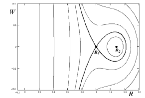
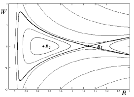
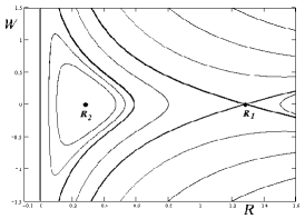
Figure 1: Phase portraits of the dynamic system (17) obtained for $\nu=0$ and $\beta=1.75$: a) $\gamma=3,\,\,s=1.6$, $R_{1}=1$; b) $\gamma=-3$, $s=1.1$, $R_{1}=1.282$; and c) $\gamma=-3$, $s=0.7$, $R_{1}=1.282$.

Fig. 1 b, plotted for $\gamma=-3$, $s=1.1$ and $R_{1}=1.282$, contains the closed loop directed towards the vertical axis. This loop corresponds to the solitary wave of rarefaction. Fig. 1 c plotted for $\gamma=-3$, $R_{1}=1.282$ and $s=0.7$ does not contain the closed loop since the inequalities (29) are not satisfied.

4 Spectral stability of the stationary solutions

In the study of spectral stability of TW solutions, it is helpful to pass to new independent variables

$$\bar{t}=t,\qquad\bar{z}=x-s\,t,$$

in which the invariant TW solutions (13) become stationary. Since the main part of the analysis is performed numerically, we confine ourselves to the case $\nu=0.$ In the new variables the system (5) reads as follows:

$$\left\{\begin{array}[]{ll}u_{\bar{t}}-s\,u_{\bar{z}}+\beta\rho\,\rho_{\bar{z}}+\gamma[\rho\rho_{\bar{z}\bar{z}\bar{z}}+3\,\rho_{\bar{z}}\rho_{\bar{z}\bar{z}}]=0,\\ \rho_{\bar{t}}-s\,\rho_{\bar{z}}+\rho^{2}u_{\bar{z}}=0,\end{array}\right.$$ (31)

(for the sake of simplicity, the bars will be omitted from now on). We restrict ourselves to the analysis of spectral stability [45, 46, 11] of the TW solution $\left(U(z),R(z)\right)$, and consider the perturbations of the following form:

$$u(t,\,z)=U(z)+\epsilon\,\exp{[\lambda\,t]}\,f(z),\qquad\rho(t,\,z)=R(z)+\epsilon\,\exp{[\lambda\,t]}\,g(z),$$ (32)

where $\lambda$ is the spectral parameter, and $|\epsilon|\ll\,1.$

Inserting the ansatz (32) into the system (31) and neglecting the $O\left(|\epsilon|^{2}\right)$ terms, we obtain the system linearized about the travelling wave solutions:

$$\begin{array}[]{l}f\lambda-sf^{\prime}+R\gamma g^{\prime\prime\prime}+\beta gR^{\prime}+3\gamma g^{\prime\prime}R^{\prime}+g^{\prime}(\beta R+3\gamma R^{\prime\prime})+g\gamma R^{\prime\prime\prime}=0,\vspace{0.1cm}\\ R^{2}f^{\prime}-sg^{\prime}+g(\lambda+2RU^{\prime})=0,\end{array}\qquad$$ (35)

where the prime denotes the derivative with respect to $z$.

Rewrite (35) as a first-order dynamical system

$$Y^{\prime}=AY,$$ (36)

where $Y=\left(g,\,\eta,\,\chi,\,f\right)^{tr}$,

$$A=\left(\begin{array}[]{cccc}0&1&0&0\\ 0&0&1&0\\ a_{1}&a_{2}&a_{3}&a_{4}\\ a_{5}&a_{6}&0&0\end{array}\right)$$

$\displaystyle a_{1}=-\frac{\beta R^{\prime}+\gamma R^{\prime\prime\prime}+R^{-2}s\left(\lambda+2RU^{\prime}\right)}{\gamma R}$, $\displaystyle a_{2}=\frac{s^{2}-\beta R^{3}-3R^{2}\gamma R^{\prime\prime}}{\gamma R^{3}}$, $\displaystyle a_{3}=-\frac{3R^{\prime}}{R}$, $\displaystyle a_{4}=-\frac{\lambda}{R\gamma}$, $\displaystyle a_{5}=-\frac{\lambda+2RU^{\prime}}{R^{2}}$, $\displaystyle a_{6}=\frac{s}{R^{2}}$. Since $R(z)$ and $U(z)$ tend to their limiting values ($R_{1}$ and $0$ respectively) as $|z|$ increases, the dynamical system under study asymptotically tends to the system with constant coefficients

$$Y^{\prime}=A_{\infty}Y,$$ (37)

where

$$A_{\infty}=\left(\begin{array}[]{cccc}0&1&0&0\\ 0&0&1&0\\ \displaystyle-\frac{s\lambda}{\gamma R_{1}^{3}}&\displaystyle\frac{s^{2}-\beta R_{1}^{3}}{\gamma R_{1}^{3}}&0&\displaystyle-\frac{\lambda}{\gamma R_{1}}\\ \displaystyle-\frac{\lambda}{R_{1}^{2}}&\displaystyle\frac{s}{R_{1}^{2}}&0&0\end{array}\right)$$

It is obvious that the linearized system (35) can be treated as a spectral problem

$$Ly=\lambda y,\qquad y=\left(f,\,g\right)^{tr},$$ (38)

for the operator

$$L=\left(\begin{array}[]{cc}-s\partial_{z}&R\gamma\partial_{z\,z\,z}+3\gamma R^{\prime}\partial_{z\,z}+(\beta R+3\gamma R^{\prime\prime})\partial_{z}+\beta R^{\prime}+\gamma R^{\prime\prime\prime}\vspace{0.1cm}\\ R^{2}\partial_{z}&2RU^{\prime}-s\partial_{z}\end{array}\right).$$

Recall that the set of all possible values of $\lambda\,\in\,\mathbb{C}$ for which the equation

$$\frac{\partial}{\partial\,t}\left[\begin{array}[]{l}\bar{u}(t,\,z)\\ \bar{\rho}(t,\,z)\end{array}\right]=L\,\left[\begin{array}[]{l}\bar{u}(t,\,z)\\ \bar{\rho}(t,\,z)\end{array}\right]$$

has nontrivial solutions of the form $\exp{[\lambda\,t]}\left[f(z),\,g(z)\right]^{tr}$ is called the spectrum $\sigma$ of the operator $L$. The homoclinic solution $\left[U(z),\,R(z)\right]^{tr}$ is said to be spectrally stable if no possible eigenvalue $\lambda$ belongs to the right half-plane of the complex plane.

Remark 1

It follows from the translation invariance of the system (31) that zero belongs to the spectrum of $L$.

As usually, we distinguish the essential spectrum $\sigma_{ess}\,\subset\,\sigma$, and the discrete spectrum $\sigma_{discr}\,\subset\,\sigma$. Being somewhat informal, we can treat $\sigma_{ess}$ and $\sigma_{discr}$ as the subsets responsible, respectively, for the stability of the stationary solutions $\left(0,\,R_{1}\right)$, and the solution $\left[U(z),\,R(z)\right]^{tr}$ itself.

Now we are going to state the conditions which guarantee that the set $\sigma_{cont}\,\bigcap\,\mathbb{C}^{+}=\emptyset$. In the limiting case $|z|\rightarrow\,\pm\,\infty$, the variational system turns into a linear system with constant coefficients,

$$-\gamma\,R_{1}\,g^{\prime\prime\prime}+s\,f^{\prime}-\beta\,R_{1}\,g^{\prime}=\lambda f,$$ (39)

$$s\,g^{\prime}-R_{1}^{2}\,f^{\prime}=\lambda\,g,\qquad$$

Location of the essential spectrum can be determined using the Fourier transform. Applying the latter to the system (39) yields

$$\hat{M}(\xi,\,\lambda)\,\left(\begin{array}[]{c}\hat{f}(\xi)\\ \hat{g}(\xi)\end{array}\right)=\left(\begin{array}[]{ll}\lambda+i\,\xi\,s,&i\,\xi\,R_{1}\,(\gamma\,\xi^{2}-\beta)\\ -i\,\xi\,R_{1}^{2},&\lambda+i\,\xi\,s\end{array}\right)\left(\begin{array}[]{c}\hat{f}(\xi)\\ \hat{g}(\xi)\end{array}\right)=0,$$ (40)

where $\hat{f}(\xi)$ and $\hat{g}(\xi)$ are respectively the Fourier transforms of $f(z)$ and $g(z)$. Equating the determinant of the matrix $\hat{M}(\xi,\,\lambda)$ to zero, we obtain the expression for eigenvalues:

$$\lambda_{1,\,2}={-\,i\,\xi\,s\,\pm\sqrt{\left(\gamma\,\xi^{2}-\beta\right)\xi^{2}\,R_{1}^{3}}},\quad\xi\,\in\,R.$$ (41)

Thus, the following assertion holds.

Statement 2

If $\gamma<0$ and $\beta>0$, then the essential spectrum $\sigma_{ess}$ does not intersect the positive half-plane $\mathbb{C}^{+}$. On the other hand, if both $\beta$ and $\gamma$ are positive, then $\sigma_{ess}$ has a non-empty intersection with $\mathbb{C}^{+}$ and the stationary solution $(0,\,R_{1})$ is unstable.

5 Numerical study of the discrete spectrum and the dynamical behavior of solitary wave solutions

An efficient tool for the study of discrete spectrum of a linearized operator is provided by the so called Evans function $E(\lambda)$, which is an analytic function of the spectral parameter $\lambda$. The zeroes of $E(\lambda)$ correspond to the eigenvalues of the linearized operators that belong to the discrete spectrum [45, 11].

The Evans function is constructed by evolving the linearized system, depending on $\lambda$, starting from the points of initiation lying at $-\infty$ in the unstable invariant manifold, and from the points at $+\infty$ lying in the stable one. The solutions (mostly extrapolated numerically) are then calculated for some fixed value of $z_{0}$ (usually for $z_{0}=0$), and the value of the Wronskian at this point determines $E(\lambda)$. If for some $\lambda_{0}$ the Evans function vanishes, then the intersection of the stable and unstable manifolds is nontrivial, there exists the corresponding eigenvector which belongs to the Hilbert space of square integrable functions $L^{2}(R)$ and, thus, $\lambda_{0}\,\in\,\sigma_{discr}.$

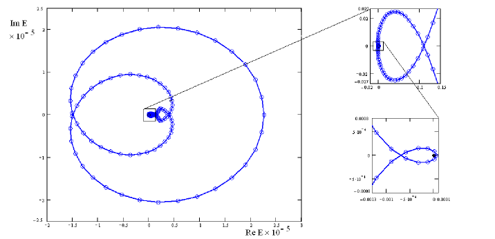
Figure 2: The real versus imaginary part of $E(\lambda)$ for $s=1.6$, $\beta=1.75$, ${\gamma=-3}$, $R_{1}=1.282$. The spectral parameter varies along the border of the half-circle with the radius $b=12$, symmetric w.r.t. the horizontal axis and separated from the vertical axis by a small offset $a=0.03$.

The analyticity of the Evans function enables to calculate the number of roots of the equation $E(\lambda)=0$, together with their multiplicities, within the compact domain $B\subset\mathbb{C}^{+}$, using the well-known formula (see e.g. [44], Ch. XV )

$$N=\sum_{j=1}^{n_{0}}k_{j}=\frac{1}{2\,\pi\,i}\,\oint_{\partial\,B}\frac{E^{\prime}(\lambda)}{E(\lambda)}d\,\lambda,$$

where $n_{0}$ is the number of roots, while $k_{j}$ is the multiplicity of the $j$-th root. The number $N$, called the winding number [46, 47, 48, 49], determines how many turns makes the vector $\left(Re{E(\lambda)},\,Im{E(\lambda)}\right)$ around the origin as $\lambda$ runs along the contour $\partial\,B$. Since we are unable to integrate numerically over an unbounded region, it is necessary to become convinced that the Evans function is nonzero for large $|\lambda|$ belonging to the positive half-plane of the complex plane (some relevant estimates are presented in Appendix 1). Thus, calculating $N$ for sufficiently large $B$ (usually $B$ is a semicircle lying in $\mathbb{C}^{+}$) and analyzing the behavior of $E(\lambda)$ for large $|\lambda|$ can give a hint regarding the location of $\sigma_{discr}.$

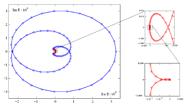
Figure 3: The real versus imaginary part of $E(\lambda)$ for $s=1.6$, $\beta=1.75$, ${\gamma=-3}$, $R_{1}=1.282$. The spectral parameter varies along the border of the half-circle with the radius $b=20$, symmetric w.r.t. the horizontal axis and separated from the vertical axis by a small offset $a=0.03$.

The construction of the Evans function is performed as follows. For large $z$ the spectral problem becomes close to the equation (37). Solutions to this equation, which are easily calculated, form at $+\infty$ a stable manifold $U^{+}$ spanned by $k$ independent eigenvectors $\left\{\vec{v_{j}}^{+}\right\}_{j=1}^{k}$ of the matrix $A_{\infty}$, corresponding to the eigenvalues $\lambda_{j}$ with the negative real part. At $-\infty$ solutions of the equation (37) form an unstable manifold $U^{-}$ spanned by $m$ independent eigenvectors $\left\{\vec{v_{j}}^{-}\right\}_{j=1}^{m}$ of the matrix $A_{\infty}$ corresponding to the eigenvalues with the positive real parts. The construction of the Evans function becomes possible when these two sets of vectors are complementary, i.e., when $m=n-k$.

So, initializing (36) with $k$ vectors $\vec{v_{j}}^{+}$ from $U^{+}$ and with $n-k$ independent vectors $\vec{v_{j}}^{-}$ from $U^{-}$ and solving the system towards $z=0$, we obtain two sets of vectors:

$$V^{-}\leavevmode\nobreak\ =\leavevmode\nobreak\ \left\{V_{1}^{-}(0,\,\lambda),\,V_{2}^{-}(0,\,\lambda),\dots,V_{n-k}^{-}(0,\,\lambda)\right\}$$

and

$$V^{+}=\left\{V_{1}^{+}(0,\,\lambda),\,V_{2}^{+}(0,\,\lambda),\dots,V_{k}^{+}(0,\,\lambda)\right\},$$

being the analytic functions of $\lambda$. These sets have nontrivial intersection if and only if $\lambda$ belongs to the discrete spectrum $\sigma_{discr}$. Therefore the analysis of zeroes of the Evans function defined as

$$E[\lambda]=\det\left[V_{1}^{-}(0,\,\lambda),\,V_{2}^{-}(0,\,\lambda),\dots,V_{n-k}^{-}(0,\,\lambda),\,V_{1}^{+}(0,\,\lambda),\,V_{2}^{+}(0,\,\lambda),\dots,V_{k}^{+}(0,\,\lambda)\right]$$ (42)

reveals the location of discrete spectrum of the operator $L$.

We perform the construction of the Evans function based on a numerical procedure. An appropriate method depends on the dimensions of invariant manifolds $U^{+}$ and $U^{-}$. In our case both stable and unstable invariant manifolds of the matrix $A_{\infty}$ happen to be two-dimensional. Prolongation of $U^{\pm}$ in multi-dimensional cases encounters the well-known obstacles [55] which can be overcome by employing the exterior algebra.

Using the wedge product we derive a $k$-form in the vector space $\wedge^{k}(\mathbb{C}^{n})$ built from the basis elements of the vector space $\mathbb{C}^{n}$. In our case $n=4$ (see Appendix 2), and the two-forms belonging to the space $\wedge^{2}(\mathbb{C}^{4})$ correspond to the invariant manifolds $U^{+}$ and $U^{-}$. As the basis we choose the vectors $w_{1}=e_{1}\wedge e_{2}$, $w_{2}=e_{1}\wedge e_{3}$, $w_{3}=e_{1}\wedge e_{4}$, $w_{4}=e_{2}\wedge e_{3}$, $w_{5}=e_{2}\wedge e_{4}$, $w_{6}=e_{3}\wedge e_{4}$. Mapping the dynamical system (36) into the space spanned by $w_{1},...w_{6}$, we obtain:

$$U^{\prime}=A^{(2)}U,$$ (43)

where

$$A^{(2)}=\left(\begin{array}[]{cccccc}0&1&0&0&0&0\\ a_{2}&a_{3}&a_{4}&1&0&0\\ a_{6}&0&0&0&1&0\\ -a_{1}&0&0&a_{3}&a_{4}&0\\ -a_{5}&0&0&0&0&1\\ 0&-a_{5}&a_{1}&-a_{6}&a_{2}&a_{3}\end{array}\right)$$

The set of eigenvalues of the matrix $A^{(2)}$ consists of all possible sums of eigenvalues of the matrix $A$. Therefore the manifolds $U^{\pm}$ are the solutions of the system (43), for which

$$\lim_{z\rightarrow\pm\infty}e^{-\mu_{\pm}z}U^{\pm}=\hat{v}^{\pm},$$

where $\hat{v}^{+}(\hat{v}^{-})$ is an eigenvector of the matrix $A^{(2)}_{\infty}$ corresponding to the eigenvalue $\mu_{+}(\mu_{-})$ with the smallest negative (largest positive) real part. The Evans function can be represented in terms of solutions $U^{\pm}$ in the following fashion [48]:

$$E(\lambda)=\exp\left\{-\int_{0}^{z}\mbox{Tr}(A^{(2)})dz\right\}U^{+}(z,\lambda)\wedge U^{-}(z,\lambda).$$ (44)

In evaluating the expression (44) we employed the relation

$$U^{+}(z,\lambda)\wedge U^{-}(z,\lambda)=\left\langle U^{-},\Sigma U^{+}\right\rangle_{R},$$

where $\langle\cdot,\cdot\rangle$ is the scalar product in the space $R^{6}$,

$$\Sigma=\left(\begin{array}[]{cccccc}0&0&0&0&0&1\\ 0&0&0&0&-1&0\\ 0&0&0&1&0&0\\ 0&0&1&0&0&0\\ 0&-1&0&0&0&0\\ 1&0&0&0&0&0\end{array}\right).$$

Below we present the steps of the procedure of computation for the Evans function. After fixing the values of the parameters corresponding to the appearance of the homoclinic loop, we choose the starting points from which we calculate the homoclinic solution. The boundary conditions at $\pm\infty$ are replaced by the boundary conditions posed at finite (sufficiently remote) points $\pm T$. The values $R(\pm T)$ and $Y(\pm T)$ should be chosen with great precision. They are obtained by solving the linearized system (17). The eigenvectors of the matrix $M_{lin}=M\left(R_{1},\,0\right)^{tr}$ (see formula (21)) are chosen in the form

$$(R(\pm T),Y(\pm T))^{tr}=(R_{1},\,0)^{tr}+\varepsilon\vec{q},$$

where $\vec{q}=\left(1,\,\mp\sqrt{\frac{-2\,E\,R_{1}-\beta R_{1}^{3}+4s^{2}}{2R_{1}^{3}\gamma}}\right)^{tr}$ are the eigenvectors of the matrix $M_{lin}$.

Figure 4: Numerical simulation of system (5) performed with $R_{1}=1.0$, $\nu=0$, $s=1.6$, $\beta=1.75$ and $\gamma=3$

The parameter $\varepsilon$ is specified by smoothly sewing the solutions starting from the initial values $z=-T$ and $z=T$. For $T=25$ we get $\varepsilon=1.885\cdot 10^{-6}$.

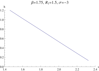
Figure 5: The dependence of the maximal depth $h$ of the solitary wave of rarefaction on the velocity $s$.

Figure 6: The dependence of the effective width $d$ of the solitary wave of rarefaction on the velocity $s$.

Next we perform a change of variables [47]

$$U=\exp\{\mu_{\pm}z\}\tilde{U},$$

that reduces the system (43) to the following form:

$$\tilde{U}^{\prime}=(A^{(2)}-\mu_{\pm}I_{4})\tilde{U}.$$ (45)

We integrate the system (45) with appropriate initial conditions from $z=+T$ to $z=+0$, and then from $z=-T$ to $z=-0$. The function $E(\lambda)$ is proportional to the $\left\langle{\tilde{U}^{-}},\Sigma{\tilde{U}}^{+}\right\rangle,$ so the zeroes of this function coincide with the zeroes of the function

$$\tilde{E}(\lambda)=\left\langle{\tilde{U}^{-}},\Sigma{\tilde{U}}^{+}\right\rangle.$$

The results obtained by the implementation of the above algorithm are presented below. In order to investigate the behavior of the Evans function within the domain lying in the positive half-plane, the Nyquist diagrams $\left(Re\,E(\lambda),\,\,Im\,E(\lambda)\right)$ are used; they enable us to fix the number of complex eigenvalues of the linearized operator $L$. We construct numerically the map $\mathbb{C}\ni\lambda\,\rightarrow\,E(\lambda)$ for $\lambda$ running along $\partial\,\Omega$, where $\Omega\in\,C^{+}$ is a closed set bounded by the straight line $z=a>0$ and the semi-circle $z=b\,\exp{i\,\pi t}$, $-\pi/2<t<\pi/2,\quad 0<a<<1<<b$ [47, 49].

The Nyquist diagrams obtained for $\gamma<0$ are shown in Figures  2 - 3. The subsequent analysis shows that the winding numbers in all these cases equal zero, so the corresponding domains do not contain the values of the spectral parameter belonging to $\sigma_{discr}$.

Figure 7: Numerical simulation of collision for two solitary waves moving towards each other. Calculations are performed for the following values of the parameters: $R_{1}=1.282,$ $\nu=0$, $s=\,\pm\,1.6$ (for the left and right perturbation correspondingly), $\beta=1.75$ and $\gamma=-3$

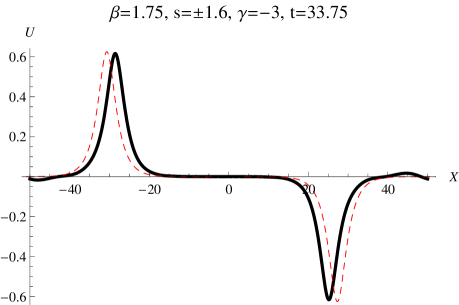
Figure 8: A “negative” phase shift attained by the solitary waves after the interaction. The dashed line represents the result of the evolution of unperturbed solitary waves. Calculated for $R_{1}=1.282,$ $\nu=0$, $s=\,\pm\,1.6$, $\beta=1.75$ and $\gamma=-3$

Figure 9: Numerical solution of the Cauchy problem for the system (5) leading to the formation of a train of solitary waves of rarefaction. Calculations are performed with the functions (49), taken as the Cauchy data, and for the following values of the parameters: $R_{1}=1.5,$ $\nu=0$, $s=1.8$, $\beta=1.75$, $\gamma=-3$, $A=19$, $B=0.35$ and $x_{0}=30$.

Now let us describe the results of numerical study of the solitary waves. The numerical experiments in which the Cauchy problem for the system (5) was solved with the solitary wave solutions taken as the initial data show that the solitary wave solutions obtained for $\gamma\,>0$ are unstable (see Fig. 4), while those corresponding to $\gamma\,<0$ are stable and evolve in a self-similar mode. It is worth noticing that the properties of the solitary waves of rarefaction supported by the system (5) are different from those of “classical” solitons. For example, the maximal depth $h$ of the solitary wave decreases when the velocity $s$ increases, see Fig. 5. On the contrary, the effective width $d$ of the wave pack measured at the depth $h/2$ nonlinearly increases as $s$ increases, see Fig. 6.

Figure 10: Numerical solution of the Cauchy problem for the system (5) at $t=160$ (solid) on the background of ”free” solitary waves (dashed), obtained at the same values of the parameters $R_{1},\,\,\gamma,\,\,\nu,\,\,\beta$, but with $s$ changing from case to case as follows: $s=1.5$ (left), $s=1.845$ (middle), $s=2.15$ (right)

Using the fact that the reduced system does not depend on the sign of velocity $s$, one is also able to choose as the Cauchy data a pair of solitary wave solutions separated with suffice spatial interval and moving toward each other. Numerical simulations show that the wave packs manifest the soliton behavior, maintaining their shape after the interaction, see Fig. 7. Note that the solitary waves of rarefaction gain the “negative” phase shift after the mutual collision, see Fig. 8.

We are also interested in finding out whether there exists a set of the initial data producing a series of solitary waves. In numerical experiments the initial data of the following form have been used:

$$\rho(0,\,x)=\left\{\begin{array}[]{c}R_{1}\quad\verb"if "\quad x<-A-x_{0},\\ R_{1}-B\left[\cos(\pi\,\frac{x+x_{0}}{A}+1)\right]\quad\verb"if "\quad-A-x_{0}\leq\,x\,\leq\,A-x_{0},\\ R_{1}\quad\verb"if "\quad x>A-x_{0},\end{array}\right.$$ (49)

$$u(0,x)=s\left(\frac{1}{R_{1}}-\frac{1}{\rho(0,\,x)}\right),\qquad\qquad\qquad\qquad\qquad\qquad\qquad\qquad\qquad\qquad$$ (50)

where $s,\,\,A,\,\,x_{0}$ and $B$ are non-negative parameters. Numerical experiments reveal the formation of the series of solitary waves of rarefaction moving with different velocities, as it is illustrated in Fig. 9. The solitons shown at this figure move from left to right, with the velocities inversely proportional to their maximal depth, which is in agreement with the above properties of the individual solitary wave of rarefaction. It occurs to be possible to choose parameters of ”free ” solitary waves in such a way that, being shifted on a proper distance, they coincide with the solitary waves of rarefaction formed in numerical solutions of the above Cauchy’s problem, Fig. 10,

6 Conclusions and discussion

In the present paper we have performed an analysis of a hydrodynamic-type system (5). In general position the system happens to admit only four symmetry generators and seven local conservation laws. The results of the symmetry analysis, as well as the study of soliton dynamics suggest that the complete integrability of the system (5) is highly unlikely, at least for the generic values of parameters.

Nevertheless, the system is shown to possess a one-parameter family of stable solitary wave solutions manifesting some features of ”true” solitons. Let us stress that existence of a one-parameter family of solitary wave solutions is connected with the employment of the dynamic equation of state (4), taking account of the effects of pure spatial non-locality. The presence of one-parametric families of localized TW solutions is rather not inherent to another known hydrodynamic-type non-local models [29], accounting for temporal [50, 51, 52] or spatio-temporal [53] non-localities. Note that throughout the text we do not use the analytical description of the solitary wave solutions. Their existence is proved on the basis of the qualitative study of the associated dynamical system. Such study is more relevant and informative than the attempts to find an analytic description for solitary waves, for they are rarely expressed in terms of elementary (or even special) functions. Moreover, applying the qualitative methods enables one to cover the whole set of invariant solutions belonging to the given family.

The main goal of this work is the study of spectral stability for solitary waves and the dynamical features thereof. A stable evolution of the solitary waves of compression corresponding to the case of $\gamma>0$ is virtually impossible because the intersection of $\sigma$ with $\mathbb{C}^{+}$ is nonempty.

In the case of $\gamma<0$ the spectrum of linearized problem happens to lie in the set $\mathbb{C}\backslash\,\mathbb{C^{+}}$. This conclusion is made on the basis of the analytic investigation of the continuous spectrum and numerical study of the Evans function performed for the selected values of parameters and covering a sufficiently large domain of the half-plane $\mathbb{C}^{+}$. These results are further backed by the estimate of the Evans function made for large $|\lambda|$ lying in the positive half-space.

A remarkable and somewhat unexpected result obtained in the numerical experiments is the elastic dynamics of interaction of solitary wave solutions. Let us stress that a mere possibility to perform such experiments is rare, for the soliton-like TW solutions supported by non-integrable evolutionary equations occur, as a rule, for specific values of parameters, including the magnitude and direction of the velocity.

The numerical studies reveal some peculiarities of the solitary waves of rarefaction, in particular, an anomalous dependence of the depth and the effective width upon the wave pack velocity. These features are well understood on the basis of qualitative analysis. The decrease of the depth of the solitary wave with the increase of the velocity is related to the properties of solutions to the algebraic equation (18) determining the horizontal coordinate of the stationary point $(R_{2},\,0)$. Thus, when the velocity $s$ obeying the inequalities (29) increases, the point $R_{2}$ in which the straight line $E\,R-s^{2}$ intersects the curve $\frac{\beta}{\nu+2}\,R^{\nu+3}$ moves towards $R_{1}$. Hence, the maximal depth of the solitary wave, which is proportional to $|R_{2}-R_{1}|$, decreases. The simultaneous increase of the effective width of the solitary wave is related to the fact that all the points of the corresponding homoclinic trajectory lie in a vicinity of the stationary points, hence the phase velocity is small in every point of the homoclinic loop and tends to zero as $s$ approaches $\sqrt{\beta\,R_{1}^{\nu+3}}$ from below.

When $s$ approaches $\sqrt{\frac{\beta(\nu+1)}{\nu+2}\,R_{1}^{\nu+3}}$ from above, a different effect is observed. Since the homoclinic loop is locked from the left by the vertical axis, it attains the shape of an equilateral triangle, symmetric w.r.t. the horizontal axis (see Fig.  1 b). Its base approaches the vertical axis, as the parameter $s$ decreases, thus resulting in an unlimited growth of the phase velocity in the region corresponding to the bottom of the solitary wave of rarefaction. This, in turn, causes the creation of an abruptly narrowing solitary wave. In fact, the solitary wave solution turns into a spike as $s$ approaches the left critical value, which is clearly seen in numerical experiments.

As a final remark, note that, in addition to obtaining the rigorous results concerning the spectral stability of the TW solution, the list of open problems for the system (5) includes the issue of more general stability and attractive features [54, 56, 57], the study of interaction of the waves for the wide range of values of parameters, and special treatment of the distinguished special case $\nu=1$, for which the system (5) possesses a nonlocal symmetry.

Appendix 1

Following a common practice [58], we shall calculate the Evans function for a system of ODEs with constant coefficients approximating the linearized system (36). Let us employ a trigonometric representation $\lambda=|\lambda|\,e^{i\,\varphi}$ for $\lambda$, assuming that $|\lambda|>>1$, and $-\frac{\pi}{2}<\varphi<\frac{\pi}{2}$. Applying the scaling transformation

$$\bar{g}=\frac{g}{R},\qquad\bar{\eta}=|\lambda|^{-1/2}\,\eta,\qquad\bar{\chi}=|\lambda|^{-1}\,\chi,\qquad\bar{f}=|\lambda|^{-1/2}\,f,$$

and passing to the new independent variable $\frac{d}{d\,\tau}=\frac{R}{|\lambda|^{1/2}}\,\frac{d}{d\,z}$, we obtain for $|\lambda|>>1$ an approximate system

$$\frac{d}{d\,\tau}\left(\begin{array}[]{c}\bar{g}\\ \bar{\eta}\\ \bar{\chi}\\ \bar{f}\end{array}\right)=\tilde{M}\,\left(\begin{array}[]{c}\bar{g}\\ \bar{\eta}\\ \bar{\chi}\\ \bar{f}\end{array}\right)=\,\left(\begin{array}[]{cccc}0&1&0&0\\ 0&0&R_{0}&0\\ 0&0&0&\frac{e^{i\,\varphi}}{\gamma}\\ e^{i\,\varphi}&D_{0}&0&0\end{array}\right)\left(\begin{array}[]{c}\bar{g}\\ \bar{\eta}\\ \bar{\chi}\\ \bar{f}\end{array}\right),$$ (51)

where $R_{0}=R(0).$

The matrix $\tilde{M}$ has four distinct eigenvalues

$$\vec{V}_{k}=\left(R_{0},\,\rho\,R_{0}\,e^{i\,\alpha_{k}},\,\rho^{3}\,e^{2\,i\,\alpha_{k}},\,\gamma\,R_{0}^{4}\,e^{i\,(3\alpha_{k}-\varphi)}\right)^{tr},$$

where $\rho=\left(R_{0}/|\gamma|\right)^{1/4}$,

$$\alpha_{k}=\frac{\varphi+(k-1)\,\pi}{2},\qquad k=1,...4.$$

Thus, in the generic case two eigenvectors belong to the unstable invariant manifold, and two other to the stable one. So the Evans function for the asymptotic problem is proportional to

$$D=R_{0}^{5}\,\det\left[\begin{array}[]{cccc}1&1&1&1\\ e^{i\,\alpha_{1}}&e^{i\,\alpha_{2}}&e^{i\,\alpha_{3}}&e^{i\,\alpha_{4}}\\ e^{2\,i\,\alpha_{1}}&e^{2\,i\,\alpha_{2}}&e^{2\,i\,\alpha_{3}}&e^{2\,i\,\alpha_{4}}\\ e^{i(3\alpha_{1}-\varphi)}&e^{i(3\alpha_{2}-\varphi)}&e^{i(3\alpha_{3}-\varphi)}&e^{i(3\alpha_{4}-\varphi)}\end{array}\right].$$ (52)

Upon performing straightforward but tedious calculations we finally obtain that

$$D=2\,i\,\,R_{0}^{5}\,e^{3\,i\,\varphi/2}\left(e^{i\,\alpha_{2}}-e^{i\,\alpha_{1}}\right)\,\left(e^{i\,\alpha_{3}}-e^{i\,\alpha_{1}}\right)\,\left(e^{i\,\alpha_{4}}-e^{i\,\alpha_{1}}\right).$$

Further analysis shows that under the above restrictions this number never vanishes, which indicates that the Evans function is nonzero for large $\lambda$ with positive real part.

Appendix 2

Consider the eigenvalues of the matrix $A_{\infty}$ corresponding to the small values of $\lambda$. The characteristic equation $\det\left[A_{\infty}-\mu\,I\right]=0$ can be written as follows:

$$\mu^{4}+\alpha_{2}\mu^{2}+\alpha_{1}\mu+\alpha_{0}=0,$$ (53)

where $\displaystyle\alpha_{2}=\frac{\beta R_{1}^{3}-s^{2}}{R_{1}^{3}\gamma}$, $\displaystyle\alpha_{1}=\frac{2s\lambda}{R_{1}^{3}\gamma}$, $\displaystyle\alpha_{0}=-\frac{\lambda^{2}}{R_{1}^{3}\gamma}$. In order to analyze the behavior of the eigenvalues for small $\lambda\not=0$, we represent the solutions of (53) in the form of series

$$\mu=\mu_{0}+\lambda\mu_{1}+\dots$$

In the zero-order approximation we obtain the equation

$$\mu_{0}^{2}\left(\mu_{0}^{2}+\alpha_{2}\right)=0.$$

This equation has a solution $\mu_{0}^{1,2}=0$ of multiplicity 2, and a pair of nonzero solutions $\mu_{0}^{3,4}=\pm\sqrt{-\alpha_{2}}$. For $\alpha_{2}<0$ or $\beta R_{1}^{3}-s^{2}>0$ the quantities $\mu_{0}^{3,4}$ are real and have different signs. For $\alpha_{2}>0$ or $\beta R_{1}^{3}-s^{2}<0$, they are purely imaginary.

The asymptotic series corresponding to nonzero $\mu_{0}^{3,4}$ has the form:

$$\mu=\mu_{0}+\frac{s}{\beta R_{1}^{3}-s^{2}}\lambda-\frac{2s^{2}+\beta R_{1}^{3}}{2(s^{2}-\beta R_{1}^{3})^{2}\mu_{0}}\lambda^{2}+\dots$$

For $\mu_{0}^{3,4}$ the expansion is different:

$$\mu=\lambda\mu_{1}+\lambda^{3}\mu_{3}+\dots,$$

where $\displaystyle\mu_{1}=\frac{1}{s\pm\sqrt{\beta R_{1}^{3}}}$, $\displaystyle\mu_{3}=\frac{\mu_{1}^{4}R_{1}^{3}\gamma}{-2s+2s^{2}\mu_{1}-2\beta\mu_{1}R_{1}^{3}}$.

When $\alpha_{2}<0\rightarrow s>\sqrt{\beta R_{1}^{3}}$ and $\lambda>0$, then the real roots are shifted to the right, while the zero roots give rise to a pair of real roots having different signs. Hence, the system (36) has a two-dimensional unstable invariant manifold. When $\alpha_{2}>0\rightarrow s<\sqrt{\beta R_{1}^{3}},$ a pair of positive roots is created from zero ones, while the pair of a pure imaginary roots gain negative real part. Thus, in this case the system (36) has two-dimensional unstable invariant manifold as well.

References

- [1] R.K. Dodd , J.C. Eilbeck, J.D. Gibbon and H.C. Morris, Solitons and Nonlinear Wave Equations, Academic Press, London 1984.
- [2] F. Lund, Interpretation of the precursor to the 1960 Great Chilean Earthquake as a seismic solitaru wave, Pure and Applied Geophysics, 121 (1983), 17-26.
- [3] R. Fitzhugh, Mathematical Model of excitation and propagation in nerve, in: Biological Engineering, H.R. Schwan ed., McGraw Hill, New York, 1969, Ch. 1, pp. 1-85.
- [4] J. Evans, Stability of nerve inpulse, Indiana Univ. Math. J., 21 (1972) 877-899.
- [5] J. Feroe, Existence and stability of multiple impulse solutions of a nerve equation, SIAM J, Appl. Math., 42 (1982) 235-246.
- [6] Ya.B. Zeldovich, Theory of Combustion and Detonation of Gases, OGIZ Academy of Sciences, Moscow, 1944 (in Russian).
- [7] A.N. Kolmogorov, I.G. Petrovsii and N.S. Piskunov, A study of diffusion equation with increase of the amount of substance and its application to a biological problem, in: V.M. Tikhomirov (Ed.) Selected works of A.N. Kolmogorov, Vol. I, Kluver, 1991, pp 242-270.
- [8] V.E. Nakoryakov, B.G. Pokusaev and I.R. Schreiber, Wave propagation in Gas-Liquid Media, CRC Publ., Boca Raton, 2011.
- [9] E.A. Demekhin, Yu. Tokarev and V.Ya. Shkadov, Hierarchy of bifurcations of space-periodic structures in nonlinear model of active dissipative media,Physica D, 52 (1991) 338-352.
- [10] B.H. Gilding and R. Kersner, Travelling Waves in Nonlinear Diffusion Convection Reaction, Birkhauser, 2004.
- [11] B. Sandstede, Stability of Travelling Waves, in: B. Fidler (Ed.), Handbook of Dynamical Systems II Elsewier (2002), pp. 983-1055.
- [12] G.B. Whitham, Linear and nonlinear waves, John Wiley & Sons Inc., 1974.
- [13] P.L. Bhatnagar, Nonlinear waves in one-dimensional dispersive systems, Clarendon Press, Oxford, 1979.
- [14] R. Nigmatulin, A.A. Gubaidullin, Amplification of shock waves in a non-equilibrium gas-liquid system, in: Y. Engelbrecht (Ed.), Nonlinear waves in active media , 1989, pp. 243-249
- [15] V.F. Nesterenko, Dynamics of Heterogeneous Materials, Springer, New York, 2001.
- [16] Ph. Rosenau, J. Hyman, Compactons: Solitons with Finite Wavlelngth, Phys Rev. Lett., 70 (1993, 564-567.
- [17] P. Olver, Ph. Rosenau Tri-Hamiltonian duality between solitons and solitary wave solutions, Phys Rev. E, 53 (1995) 1900-1906.
- [18] J. Vodová A complete List of Conservation Laws for Non-integrable Compacton Equations of type , 26 (2013) 757–762 (arXiv:1206.440v1 [nlin.SI])
- [19] Makhan’kov V.G., Solitons and Numerical Experiments, Physics of Elementary Particles and Atomic Nuclei, 14 (1983) 123-180 (in Russian).
- [20] Makhan’kov V.G., Soliton Phenomenology, Springer, New York, 1990.
- [21] Nesterenko V.F., Propagation of Nonlinear Compression pulses in Granular Media, J. Appl. Mech. and Tech. Phys., 5 (1983) 733-743.
- [22] Nesterenko V.F., Dynamics of Heterogeneous Materials, Springer, New York, 2001.
- [23] Pikovsky A., Rosenau Ph., Phase Compactons, Physica D, 218 (2006) 56-69.
- [24] Rosenau Ph., Pikovsky A., Phase Compactons in Chains of Dispersevly Coupled Oscillators, Phys Rev. Lett., 94 (2005) 174102.
- [25] Kurkiina O.E., Kurkin A.A., Ruvinskaya E.A. et al., Dynamics of solitons supported by the nonintegrable version of the Korteweg-de Vries equation, Pis’ma v Zhurnal Eksperimental’noj i Teoreticheskoj Fiziki, 95 (2012) 98-103 (in Russian).
- [26] V.A. Danylenko, V.V. Sorokina and V.A. Vladimirov, Journal of Physics A: Math & Gen 26 (1993) 7125-7135.
- [27] Makarenko A, Mathematical modelling of memory effets influence on fast hydrodynamic and hat conducting processes, Control and Cybernetics, 25 (1996) 621-630.
- [28] Peerlings RHJ Geers MGD Borst R et al., A critical comparison of nonlocal and gradient-enhanced softening continua, Int. J. of Solids and Structure, 38 (2001) 7723-7746.
- [29] V.A. Danylenko, T.B. Danevych, O.S. Makarenko, S.I. Skurativskyi and V.A. Vladimirov, Self-Organization in Nonlocal Non-Equilibrium Media, Subbotin Institute of Geophysics, Kyiv, 2011.
- [30] R.H.J. Peerlings, Enhanced damage modeling for fracture and fatigue, Ph.D. dissertation, Technische Universiteit, Eindhoven, 1999.
- [31] V.A. Vladimirov, E.V. Kutafina, On the localized invariant solutions of some nonlocal hydrodynamic-type model, in A. Nikitin, V Boyko (Eds.), Proc. of V Int. Conf. ”Symmetry in Nonlinear Mathematical Physics”, Part 3 (2004), 1510-1515 (http://www.slac.stanford.edu/econf/C0306234/papers/vladimirov.pdf)
- [32] V.A. Vladimirov, E.V. Kutafina and B. Zorychta, On the nonlocal hydrodynamic-type system and its soliton-like solutions, J. Phys. A: Math. Theor., 45 (2012) 085210.
- [33] V.A. Vakhnenko and V. V. Kulich, Long-wave processes in periodic media, J. Appl. Mech. Techn. Physics 32 (1992) 814
- [34] V.A. Vakhnenko, V.A. Danylenko and A. Michtchenko, An asymptotic averaged model of nonlinear long waves propagation in media with a regular structure, Int. J. Nonl. Mech., 34 (1999) 643-654.
- [35] Rudyak VYa 1987 Statistical Theory of Dissipative Processes in Gases and Liquids, Nauka Publ., Novosibirsk, 1987 (in Russian).
- [36] Zubarev D., Tishchenko S., Physica, 50 (1972) 285
- [37] N. Ari, A.C. Eringen, Nonlocal stress Field and Griffith crack, Cryst. lattice Def. Amorph. Math., 10 (1983) 33-38.
- [38] P.J. Olver, Applications of Lie groups to differential equations, 2nd ed., Springer, New York, 2000.
- [39] G. Bluman, S. Anco and A. Cheviakov, Applications of Symmetry Methods to Partial Differential Equations, Springer, New York, 2010.
- [40] N.H. Ibragimov, Transformation groups applied to mathematical physics, Reidel, Boston, 1985.
- [41] A.S. Fokas, Symmetries and integrability, Stud. Appl. Math., 77 (1987) 253–299.
- [42] A.V. Mikhailov, A.B. Shabat, V.V. Sokolov, The symmetry approach to classification of integrable equations, in V.E. Zakharov (Ed.), What is integrability?, Springer, Berlin, 1991, pp. 115–184
- [43] D. Henry, Geometric theory of semilinear parabolic equations, Springer-Verlag, Berlin, 1981.
- [44] K. Maurin, Analysis, PWN, Warsaw, 1992.
- [45] J. Evans, Nerve axon equations. III: stability of the nerve impulse, Indiana Univ. Math. J., 22 (1972) 577-593.
- [46] J. Evans, Nerve axon impulse IV: the stable and unstable impulse, Indiana Univ. Math. J., 24 (1975) 1169-1190.
- [47] T.J. Bridges, G. Derks, G.A. Gottwald, Stability and instability of solitary waves of the fifth-order KdV equation: a numerical framework, Physica D, 172 (2002) 190-216.
- [48] G. Derks, G.A. Gottwald, A robust numerical method of study oscillatory instabilty of gap solitary waves, SIAM J. Appl. Dyn. Sys. , 4 (2005) 140-158.
- [49] E. Blank, T. Dohnal, Families of surface gap solitons and their stability via the numerical Evans function method, SIAM J. Appl. Dyn. Sys., 10 (2011) 667-706.
- [50] V. Vladimirov, Compacton-like solutions of the hydrodynamic system describing relaxing media, Rep. Math. Physics, 61 (2008) 380-400.
- [51] V. Danylenko, V. Vladimirov, Qualitative and numerical study of the non-equilibrium high-rate processes in relaxing media, Control and Cybernetics, 25 (1996) 569-581.
- [52] V. Vladimirov, A. Mahdi al Dhayeh, Normal forms application for studying solitary wave solutions of non-integrable evolution systems, Comm. in Nonl. Science and Num. Simul., 9 (2004) 615-631.
- [53] V. Vladimirov, S. Skurativsky, Soliton-like solutions and other wave patterns in the nonlocal models of structured media, Rep. Math. Physics, 46 (2000) 287-294.
- [54] G. I. Barenblatt, Similarity, Self-similarity and Intermediate Asymptotics, Consultants Bureau, New York, 1979.
- [55] L. Allen, Th. J. Bridges, Numerical exterior algebra and the compound matrix method, Numerische Mathematik, 9 (2002) 197-232.
- [56] S. Kamin and Ph. Rosenau, Energence of waves in a nonlinear convection-reaction-diffusion equation, Advanced Nonlinear Studies, 4 (2004) 251-272.
- [57] S. Kamin and Ph. Rosenau, Convergence to the traveling wave solution for a nonlinear reaction-diffusion equation, Rendiconti Mat. Acc. Lincei, 15 (2004) 271-280.
- [58] J. Humpherys, K. Zumburn, An efficient schooting algorithm for Evans function calculations in large systems, Physica D, 220 (2006) 116-130.