Weyl meson and its implications in collider physics and cosmology

Abstract

Local scale invariant theory leads to the existence of a new particle called the Weyl vector meson. We study a generalized Standard Model, which displays local scale invariance. The model contains a real scalar field, besides the Higgs multiplet and coupling between the Higgs and Weyl meson. For certain range of coupling parameters, the Weyl-Higgs coupling leads to interesting phenomenon in particle colliders as well as in cosmology. Here we study the signature of the Weyl meson in particle colliders and determine the range of coupling parameters for which it can solve the dark matter problem.

I Introduction

One of the major unsolved problems in modern physics is the dark matter and the dark energy. The idea of dark matter came up with the discovery of inconsistency in galactic rotation curves and in analysis of galaxy clusters oort ; zwiky ; zwiky1 ; rubin . Whereas, the dark energy is required in order to explain the accelerated expansion of the Universeriess ; perlmutter . Observations shows that $23\%$ of total energy density of the Universe is in the form of dark matter, $72\%$ is dark energy and rest is ordinary matterwmap1 . All of our scientific studies are related with this ordinary visible matter, which is a very small fraction of the Universe. The dark components of the Universe are still not well understood. There are many theoretical models dealing with dark energy, but here our main concern is the dark matter. There currently exist many dark matter candidates bertone ; jungman ; bergstrom ; feng ; Bertone1 . One interesting possibility is the Weyl meson which arises naturally in local scale invariant theories. This symmetry was introduced by H. Weyl in 1929 weyl , and the gauge particle associated with this symmetry is called the Weyl meson. Local scale invariance has been reviewed by many authors dirac ; sen ; utiyama ; utiyama1 ; Freund1 ; hayashi ; hayashi1 ; nishioka ; ranganathan ; rajpoot ; rajpoot1 and the mechanism for breaking this symmetry has been discussed in Refs. jain1 ; pseudoscale ; brokenscale . In Refs. cheng ; hcheng , it has been shown that the Weyl meson acts as a dark matter candidate in a locally scale invariant generalization of the Standard Model. Cosmological implications of Weyl meson in this theory, which contains only one Higgs doublet, have been studied in jain1 ; DEDM ; huang ; wei . But in this model Higgs particle get eliminated from the particle spectrum, which leads to violation of perturbative unitarity beyond electroweak scale, as shown in Refs. joglekar ; cornwall . Hence this model needs to be generalized.

In Ref.quantumweyl a generalization of this model has been proposed by including an additional real scalar field $\chi$. In this generalized locally scale invariant Standard Model, the Higgs like particle remains in the physical spectrum and also couples directly with the Weyl meson. This model respects the unitarity condition and hence is perturbatively stable. The phenomenological implications of this model are also very interesting and need to be studied in detail, which is the main motive of this work.

In this paper we started with the model described in Ref.quantumweyl , which contains the coupling between the Weyl meson and the Higgs boson. The Weyl meson, which interacts only with the Higgs particle and no other SM particle, may serve as a good candidate for the dark matter. To strengthen this possibility we have to look for the processes, involving the Weyl meson, at the colliders and also in the Universe. The coupling strength, which plays a crucial role in all these processes, is determined by the free parameters of the theory, $f$ and $\beta_{1}$. We write the parameter $f$ in the term of Weyl meson’s mass $M_{S}$ as, $M_{S}\approx fm_{pl}$ . Now our free parameters are $\beta_{1}$ and $M_{S}$. For the model introduced by Cheng cheng , there is a cosmological constraint on the mass of the Weyl meson as shown in Ref.huang . Here we do not consider any unitarity bound on the mass of Weyl meson. Our main goal in this paper is to put some constraint on the value of coupling parameters $\beta_{1}$ and mass $M_{S}$ so that the Weyl meson can act as a suitable dark matter candidate.

This paper is organised as following. In Sec. II we start with generalized local scale invariant Standard Model and write down the interaction Lagrangian for Weyl meson. We discuss the implications of Weyl meson at colliders. For that we calculate the Higgs production cross section at Large Hadron Collider (LHC) by including these interaction term. In Sec. III we consider the Weyl meson as dark matter candidate and find the possible values of parameters for which it has relic density equal to dark matter energy density. In Sec. IV we further constrain these values by demanding the life time of Weyl meson to be equal or greater than the age of Universe. Finally we conclude in Sec. V.

II Weyl meson and Higgs boson production at LHC: Implication of generalized local scale invariant Standard Model

The action for the generalized locally scale invariant Standard Model, including an additional real scalar field $\chi$, may be written as quantumweyl ; shapo

$$\begin{split}\mathcal{S}=\int&d^{4}x\sqrt{-\bar{g}}\left(\left[\frac{\beta}{8}\chi^{2}+\frac{\beta_{1}}{4}{\mathcal{H}^{\dagger}}\mathcal{H}\right]{\bar{R}}^{\prime}\right.\\ &\left.+{\bar{g}}^{\mu\nu}\left(D_{\mu}\mathcal{H}\right)^{\dagger}\left(D_{\nu}\mathcal{H}\right)+\frac{1}{2}{\bar{g}}^{\mu\nu}\left(D_{\mu}\chi\right)\left(D_{\nu}\chi\right)\right.\\ &\left.-\frac{1}{4}\lambda\chi^{4}-\frac{1}{4}\lambda_{1}\left[2{\mathcal{H}^{\dagger}}\mathcal{H}-{\lambda_{2}}{\chi}^{2}\right]^{2}\right)\end{split}$$ (1)

Here $\mathcal{H}$ is the Higgs doublet denoted as $\mathcal{H}=\mathcal{H}_{0}+\mathcal{\hat{H}}$, $\mathcal{H}_{0}$ is the classical solution to the Higgs field, given as

$$\mathcal{H}_{0}=\frac{1}{\sqrt{2}}\left(\begin{array}[]{c}0\\ v\end{array}\right).$$ (4)

We can parameterize the $\mathcal{\hat{H}}$ in such a way that only its $\phi_{3}$ component is non-zero. The scale-covariant curvature scalar,${\bar{R}}^{\prime}$, is defined in Ref.donoghue and $D_{\mu}$ is the scale-covariant derivative defined as

$$D_{\mu}=\partial_{\mu}-fS_{\mu},$$ (5)

where $f$ is the gauge coupling constant and $S_{\mu}$ is the Weyl meson field. The field $\chi$ in this model is a singlet under electroweak symmetry transformations. The potential shown in Eq.(1) is stable due to underlying scale symmetry and also quantum corrections will not lead to any fine tuning problems, as shown in Ref.shapo . By making the quantum expansion of the fields around its classical values,

$$\begin{split}\chi&=\chi_{0}+\hat{\chi},\;\;\;\;\;\;\phi_{3}=\phi_{3,0}+\hat{\phi_{3}}\\ \bar{g}_{\mu\nu}&=g_{\mu\nu}+h^{\prime}_{\mu\nu}\ ,\end{split}$$ (6)

we can extract the quadratic mass and mixing terms of the fields. The classical value of the field $\chi$ is taken of the order of Planck’s mass and the graviton field is redefined,

$$h^{\prime\beta}_{\alpha}={4\over\sqrt{\beta\chi_{0}^{2}+\beta_{1}v^{2}}}h^{\beta}_{\alpha}\ ,$$ (7)

so that its kinetic energy term gets properly normalized. Detailed quantum treatement of this model has been discussed in Ref.quantumweyl . There it was shown that after choosing a proper gauge one can eliminate the mixing terms and identify the mass term of Weyl meson as,

$$M_{S}^{2}=f^{2}\left[\chi_{0}^{2}\left(1+\frac{3\beta}{2}\right)+v^{2}\left(1+\frac{3\beta_{1}}{2}\right)\right].$$ (8)

Remaining terms of the action can be arranged in a matrix form as $\Phi^{T}M^{2}\Phi/2$, where

$$\Phi=\left(\begin{array}[]{c}\hat{\chi}\\ \phi_{3}\\ h\end{array}\right),$$ (12)

is a scalr field triplet and $M$ is the mass matrix of this scalar field, which may be decomposed into unperturbed and perturbed parts as,

$$M^{2}=M_{0}^{2}+\Delta M^{2}.$$ (13)

The diagonalization of unperturbed mass matrix, considering only leading order terms, gives three eigenvalues which can be identified with the mass of Goldstone type mode, Higgs particle and graviton, with the eigen functions as $\tilde{\chi}$, $\tilde{\phi_{3}}$ and $\tilde{g}$, respectively. Now we can write the action in term of these particles by inverse transformation. Here we are interested only in the interaction terms for the Higgs and the Weyl meson. These arise from kinetic energy term of Higgs boson and coupling of Higgs with gravity in the action. So we can write the interaction Lagrangian as quantumweyl ,

$$\begin{split}\mathcal{L}_{int}=&\frac{3}{4}f\beta_{1}[\tilde{\phi}_{3}{}^{2}S^{\mu}_{;\mu}+2vf\tilde{\phi}_{3}S^{\mu}S_{\mu}+f\tilde{\phi}_{3}{}^{2}S^{\mu}S_{\mu}]\\ &-fS^{\mu}\tilde{\phi_{3}}\partial{\tilde{\phi}_{3}}+f^{2}v\tilde{\phi_{3}}S_{\mu}S^{\mu}+\frac{1}{2}f^{2}\tilde{\phi_{3}}^{2}S^{\mu}S_{\mu}.\end{split}$$ (14)

So far the values of parameters $f$ and $\beta_{1}$ are unconstrained. For application to collider physics, we assume that $f$ is sufficiently small and $\beta_{1}$ is sufficiently large such that $f\beta_{1}$ is of order unity. In this case the mass of Weyl meson is small and it may produce observable effects at colliders such as LHC. We only need to consider the first term in Eq.(14). It may be represented diagrammatically as,

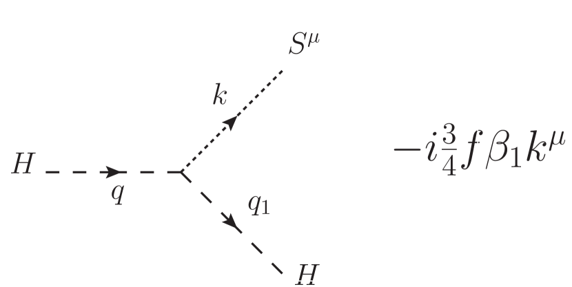
Figure 1: Higgs-Weyl meson Interaction.

II.1 Real Weyl meson production at LHC

The Weyl meson may be produced at LHC through its interaction with the Higgs particle. At LHC gluon-gluon fusion is the dominant process for the Higgs production Dawson ; collider . The corresponding Feynman diagram for Weyl meson production is shown in Fig.2.

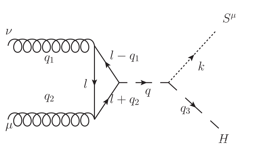
Figure 2: Production of Higgs Boson and real Weyl meson at LHC.

Let $\epsilon_{\mu}$ be the polarisation vector of the outgoing Weyl meson, then the matrix element for this process can be written as,

$$\mathcal{M}\propto k^{\mu}\epsilon_{\mu}\\ ,$$

hence,

$$\sum|\mathcal{M}|^{2}\propto\sum|k^{\mu}\epsilon_{\mu}|^{2}=0\\ ,$$

due to transversality condition chengli ; collider for real vector meson. Hence no real Weyl meson can be produced for this type of interaction at colliders.

II.2 Virtual Weyl meson and associated Higgs boson production at LHC

We have found that the amplitude for real Weyl meson production at LHC is zero. However the probability to produce a virtual Weyl meson may not be negligible. This might allow us to indirectly infer its presence at LHC. Here we consider the Weyl meson produced as an intermediate virtual particle, which gives two real Higgs bosons as the final particles. This will lead to three Higgs production at LHC. We consider only the leading order diagrams of this process, shown in Fig.3

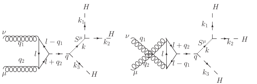
Figure 3: Virtual Weyl meson and three Higgs production at LHC.

The Higgs and the Weyl meson’s propagators can be written as quantumweyl

$$\text{Higgs boson}\,-----\quad\frac{-i}{q^{2}-m_{H}^{2}}$$ (15)

$$\text{Weyl Meson}\;........\quad\frac{-i}{k^{2}-M_{S}^{2}+i\epsilon}\left(g_{\mu\nu}-\frac{k_{\mu}k_{\nu}}{M_{S}^{2}}\right)$$ (16)

Here we write the Weyl meson’s propagator in unitary gauge. Using these propagators the complete scattering matrix element for this process can be written as,

$$\begin{split}\mathcal{M}=&(-ig_{s})^{2}(\frac{-iy_{t}}{\sqrt{2}})i^{3}Tr[t_{a}t_{b}]\epsilon_{\nu}(\lambda_{1},q_{1})\,\epsilon_{\mu}(\lambda_{2},q_{2})\int\frac{d^{4}l}{(2\pi)^{4}}\frac{1}{D_{1}D_{2}D_{3}}\,Tr\left[(\not{l}+\not{q_{2}}+m)\gamma^{\mu}(\not{l}+m)\gamma^{\nu}(\not{l}-\not{q_{1}}+m)\right.\\ &\left.+(-\not{l}+\not{q_{1}}+m)\gamma^{\nu}(-\not{l}+m)\gamma^{\mu}(-\not{l}-\not{q_{2}}+m)\right]\frac{-i}{q^{2}-m_{H}^{2}}\left(-i\frac{3}{4}f\beta_{1}k^{\alpha}\right)\,\frac{-i}{k^{2}-M_{S}^{2}+i\epsilon}\left(g_{\mu\nu}-\frac{k_{\alpha}k_{\beta}}{M_{S}^{2}}\right)\left(-i\frac{3}{4}f\beta_{1}k^{\beta}\right),\\ \end{split}$$ (17)

where

$$\begin{split}D_{1}&=l^{2}-m^{2},\quad D_{2}=(l-q_{1})^{2}-m^{2},\\ D_{3}&=(l+q_{2})^{2}-m^{2}.\end{split}$$

Here $m$ is the mass of quark in the loop and the most dominant contribution comes from the top quark. We follow the procedure given in Ref.bentvelsen to do the loop integration over $l$ and get

$$\begin{split}\mathcal{M}=\mathcal{M}_{1}\frac{-i}{q^{2}-m_{H}^{2}}&\left(-i\frac{3}{4}f\beta_{1}k^{\alpha}\right)\,\frac{-i}{k^{2}-M_{S}^{2}}\\ &\left(g_{\mu\nu}-\frac{k_{\alpha}k_{\beta}}{M_{S}^{2}}\right)\left(-i\frac{3}{4}f\beta_{1}k^{\beta}\right),\\ \end{split}$$ (18)

where

$$\begin{split}\mathcal{M}_{1}&=a(\epsilon_{1}.\epsilon_{2}-\frac{2}{\hat{s}}a(\epsilon_{1}.q_{2})(\epsilon_{2}.q_{1})\\ a&=\frac{m}{2\pi^{2}}\left[1+(1-\lambda)f(\lambda)\right]\\ \end{split}$$

and $\epsilon_{i}=\epsilon_{\mu}(\lambda_{i},k_{i})$ are the polarisation vector of the gluons having spin state $\lambda_{i}$. We average over initial spin state of protons and colour states of gluons. Furthermore $g_{s}^{2}=8\pi\alpha_{s}$ and $\frac{y_{t}}{\sqrt{2}}=(\sqrt{2}G_{f}m^{2})^{1/2}$. The colour trace term is $Tr[t_{a}t_{b}]=\frac{1}{2}\delta_{ab}$. After putting all these factors and summing over spin state of gluons $\lambda_{1},\lambda_{2}$, we get the squared amplitude for this process as,

$$\sum_{\lambda_{1},\lambda_{2}}|{\mathcal{M}}|^{2}=\frac{G_{f}\,\alpha_{s}^{2}\,\hat{s}^{2}}{288\sqrt{2}\pi^{2}}\left(\frac{3}{4}f\beta_{1}\right)^{4}\,\frac{|A(\lambda)|^{2}\left[s_{12}-\frac{s_{12}^{2}}{M_{S}^{2}}\right]^{2}}{(\hat{s}-m_{H}^{2})^{2}(s_{12}-M_{S}^{2})^{2}},$$ (19)

where Mandelstam variables are defined as,

$$\hat{s}=(q_{1}+q_{2})^{2}=q^{2},\quad s_{12}=(k_{1}+k_{2})^{2}\,=k^{2}$$ (20)

and

$$\begin{split}\lambda&=\frac{4m^{2}}{\hat{s}},\quad\beta=\sqrt{1-\lambda}\\ A(\lambda)&=\frac{3}{2}\lambda[1+(1-\lambda)f(\lambda)]\\ f(\lambda)&=\left\{\begin{array}[]{l c}arcsin^{2}(\frac{1}{\sqrt{\lambda}})\qquad\lambda\geq 1\\ -\frac{1}{4}\left[ln(\frac{1+\beta}{1-\beta})-i\pi\right]\qquad\lambda<1.\end{array}\right.\end{split}$$ (21)

II.3 Cross-Section

The cross-section for this process at parton level can be written in CM frame as halzen ,

$$\begin{split}\hat{\sigma}&=\frac{1}{2\hat{s}}\int\sum|\mathcal{M}|^{2}d\Phi_{3},\end{split}$$ (22)

where $d\Phi_{3}$ is the three-body phase space.

Three body phase space integration can be done easily by decomposing it into two body phase space integral (see e.g phase ; hitoshi ).

Total cross-section for this process is given by

$$\sigma=\int dx_{1}dx_{2}f(x_{1})f(x_{2})\hat{\sigma},\\$$ (23)

where $x_{1}$ and $x_{2}$ are momentum fraction of gluons and $\hat{s}(=sx_{1}x_{2}$) is the square of total CM energy of the system at parton level. Taking $x_{1}x_{2}=T$ and $x_{2}$ as the independent variables collider , the total cross-section become

$$\sigma=\int_{\frac{9m_{H}^{2}}{s}}^{1}dT\int_{T}^{1}\,\frac{dx_{2}}{x_{2}}f(\frac{T}{x_{2}},Q)\,f(x_{2},Q)\,\hat{\sigma}\\$$ (24)

Here $f(x,Q)$ is the parton distribution function(PDF) for the gluons. We also find the differential cross-section for this process to see the behaviour at on mass-shell condition of Weyl meson,

$$\frac{d\sigma}{ds_{12}}=\int_{\frac{9m_{H}^{2}}{s}}^{1}dT\int_{T}^{1}\,\frac{dx_{2}}{x_{2}}f(\frac{T}{x_{2}},Q)\,f(x_{2},Q)\,\frac{d\hat{\sigma}}{ds_{12}}.$$ (25)

The differential cross-section for the three Higgs production, $d\sigma/dS_{12}$, is shown in Fig.4. The total cross-section, $\sigma$, is shown in Fig.5. In these calculations we have used the CTEQ PDFs.

We calculated the three Higgs production cross-section by setting $f\beta_{1}=1$, which is the maximum allowed value of the coupling within the perturbation region. It is clear from Fig.4 that the differential cross-section varying smoothly with $S_{12}$ even in the vicinity of $S_{12}=M_{S}^{2}$. This is because the production cross-section for real Weyl meson is negligible in this theory.

We find in Fig.5 that the total cross-section for three Higgs production varies from $1pb$ at $M_{S}\approx 10\,GeV$ to $10^{-8}pb$ at $M_{S}\approx 1200\,GeV$. Hence the cross-section falls

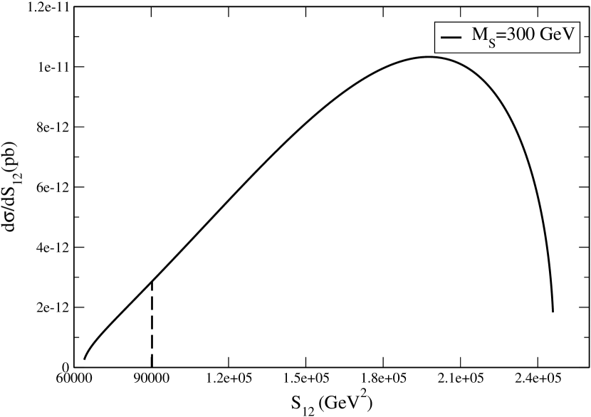
Figure 4: Differential cross-section of three Higgs production at 7 TeV of CM energy for $M_{S}=300GeV$. The dashed line in this figure indicates the position where $S_{12}=M_{S}^{2}$.

Figure 5: Leading order three Higgs production cross-section at 7 TeV of CM energy for $m_{H}=126GeV$.

sharply with increase in the mass of the Weyl meson. For comparison, the production cross-section for single Higgs boson with $m_{H}=126$, is roughly $3pb$. Hence for small values of the Weyl meson mass, the three Higgs production cross-section is not negligible compared to single Higgs cross-section. The background to the three Higgs cross-section would arise from the top quark loop. This will include two additional vertices of top quark with the Higgs boson. Hence the process is suppressed by $(\alpha_{Yt})^{2}\approx 10^{-2}$, compared to single Higgs production. We, therefore, conclude that for small $M_{S}<100\,GeV$, it may be possible to extract the contribution due to Weyl meson to three Higgs production cross-section at LHC.

III Weyl meson as a Dark Matter Candidate

The Weyl meson acts as a dark matter candidate since it interacts only with Higgs boson and no other SM particles. In Sec. II we wrote down the various interaction terms for Weyl meson. At very early time in the Universe, when temperature was very high, Weyl Meson may remain in thermal equillibrium with other particles by these interactions. Its number density keeps on changing by the coannihilation process. But as the temperature of the Universe drops down to certain level, due to expansion, its interaction rate become less than the expansion rate and coannihilation process ceases. It gets decoupled from other particles and its number density freezes out at this temperature and remains as relic density. In this section we calculate the coannihilation rate of the Weyl meson and find the possible values of parameters $\beta_{1}$ and $M_{S}$ by constraining its abundance equal to the observed dark matter abundance.

III.1 Coannihilation rate of the Weyl meson

We consider only the dominant processes which will contribute to the total coannihilation rate of the Weyl meson, as shown in Fig.6.

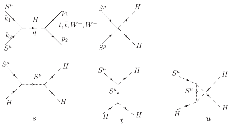
Figure 6: Weyl meson annihilation processes.

Interaction rate for annihilation process can be written as

$\qquad\Gamma=n_{eq}<\sigma v>$,

where $<\sigma v>$ is the thermally averaged annihilation cross section given by, gondolo ; gondolo1

$$<\sigma v>=\frac{g_{s}^{2}T}{32n_{eq}^{2}\pi^{4}}\int_{4m_{s}^{2}}^{\infty}ds\,\sigma\left(P_{12}^{2}\,\sqrt{s}\right)\,K_{1}\left(\frac{\sqrt{s}}{T}\right).$$ (26)

Here $K_{1}(x)$ is the modified Bessel function of second kind of order one, $T$ is the temperature at which proces is occuring, $g_{s}$ is the number degrees of freedom of the Weyl meson and $P_{12}$ is the four momentum in center of mass frame of incoming particles, which is given by

$$P_{ij}=\frac{\sqrt{s}}{2}\sqrt{1-2\left(\frac{m_{i}^{2}+m_{j}^{2}}{s}\right)+\frac{(m_{i}^{2}-m_{j}^{2})^{2}}{s^{2}}}.$$ (27)

Let $\epsilon$ be the polarisation vector of incoming Weyl meson, then the scattering amplitude for annihilation of two Weyl meson into fermion pair can be written as

$$\mathcal{M}_{1}= \frac{3}{2}\,f^{2}\,\beta_{1}(\sqrt{2}G_{f})^{\frac{1}{2}}m_{t}\epsilon_{\mu}\epsilon_{\mu}$$

$$*\left(\frac{-i}{q^{2}-m_{H}^{2}+im_{H}\varGamma_{t}}\right)\bar{u}(p_{1})v(p_{2})$$ (28)

$$\sum_{spin}|{\mathcal{M}_{1}}|^{2}= \frac{1}{4}\left(\frac{(f^{2}\beta_{1}v)^{2}\sqrt{2}G_{f}m_{t}^{2}}{(s-m_{H}^{2})^{2}+m_{H}^{2}\varGamma_{t}^{2}}\right)\left(\frac{s^{3}}{2M_{S}^{4}}\right)$$

$$*(1+12\lambda_{s}^{2}-4\lambda_{s})(1-4\lambda_{b}),$$ (29)

where $\lambda$ is defined as,

$\lambda_{i}=\frac{M_{i}^{2}}{s}$.

The top quarks, being massive, will have the dominant contribution in this case. Now we can write the cross section for this process in CM frame of incoming particles,

$$\sigma= \frac{\sum|{\mathcal{M}_{1}}|^{2}\sqrt{1-4\lambda_{b}}}{32\pi P_{12}\sqrt{s}},\;P_{12}=\frac{\sqrt{s}}{2}\sqrt{1-\frac{4M_{S}^{2}}{s}}.$$ (30)

Hence the resulting coannihilation rate for this process become

$$\Gamma_{1}= \frac{g_{s}^{2}(f^{2}\beta_{1}v)^{2}G_{f}m_{t}^{2}T}{8192\sqrt{2}\pi^{5}M_{S}^{4}n_{eq}}$$

$$\int_{4M_{S}^{2}}^{\infty}ds\frac{s^{\frac{7}{2}}\sqrt{1-4\lambda_{s}}(1-4\lambda_{s}+12\lambda_{s}^{2})}{(s-m_{H}^{2})^{2}+m_{H}^{2}\varGamma_{t}^{2}}K_{1}(\frac{\sqrt{s}}{2}).$$ (31)

For numerical integration, we change the variable $s$ to $x$ as,

$$\frac{s}{4T^{2}}-\frac{M_{S}^{2}}{T^{2}} =x^{2}$$ (32)

$$\frac{M_{S}}{T}=y$$ (33)

and write the expression for $n_{eq}$ in term of modified Bessel function of second kind of order two ($K_{2}(x)$) (see drees )

$$n_{eq}=\frac{g_{s}}{2\pi^{2}}TM_{S}^{2}K_{2}(y).$$ (34)

We can simplify the expression for coannihilation rate in the limit $s>>m_{H}^{2}$, as we are considering these process very early in the Universe, when temperature was very high. Considering only those terms which are linear in $\lambda_{i}$ results in coannihilation rate

$$\Gamma_{1}=\frac{g_{s}(f^{2}\beta_{1}v)^{2}G_{f}m_{b}^{2}T}{64\sqrt{2}\pi^{3}M_{S}K_{2}(y)y^{5}}\int_{0}^{\infty}dx\,x^{4}K_{1}\left(2\sqrt{x^{2}+y^{2}}\right).$$ (35)

Similarly we can write the coannihilation rate for second process, where Weyl meson annihilate into the Higgs pair, as

$$\Gamma_{2}=\frac{g_{s}M_{S}\left(f^{2}\beta_{1}\right)^{2}}{256\pi^{3}K_{2}(y)y^{7}}\int_{0}^{\infty}dx\,x^{4}\left(x^{2}+y^{2}\right)^{2}K_{1}\left(2\sqrt{x^{2}+y^{2}}\right).$$ (36)

Next process is the annihilation of Weyl meson with Higgs particle, for which we have $s,t$ and $u$ channel processes. Matrix element of these processes will be sum of all these channels, i.e $\mathcal{M}=\mathcal{M}_{s}+\mathcal{M}_{t}+\mathcal{M}_{u}$
where

$$\mathcal{M}_{s} =\frac{9}{8}f^{3}\beta_{1}^{2}v\left(\frac{\epsilon_{\mu}}{(s-M_{S}^{2})}(g^{\mu\nu}-\frac{k^{\mu}k^{\nu}}{M_{S}^{2}})k_{\nu}\right)$$

$$=\frac{9}{8}f^{3}\beta_{1}^{2}v\left(\frac{(\epsilon.k)(1-\frac{s}{M_{S}^{2}})}{(s-M_{S}^{2})}\right)$$

$$=-\frac{9}{8}f^{3}\beta_{1}^{2}v\frac{\epsilon.k_{s}}{M_{S}^{2}}.$$ (37)

Similarly for other channels

$$\mathcal{M}_{t}=-\frac{9}{8}f^{3}\beta_{1}^{2}v\frac{\epsilon.k_{t}}{M_{S}^{2}},\;\;\mathcal{M}_{u}=-\frac{9}{8}f^{3}\beta_{1}^{2}v\frac{\epsilon.k_{u}}{M_{S}^{2}}.$$ (38)

We used the subscript on $k$ to define it in different channels.

The amplitude of this process contains square term of each channel’s matrix element and also the cross terms, which we can write by using

$$(\epsilon.k_{s})(\epsilon.k_{t})=\frac{(p.k_{s})(p.k_{t})}{M_{S}^{2}},$$

and

$$(\epsilon.k_{s})^{2} =k_{s}^{\mu}(-g_{\mu\nu}+\frac{p_{\mu}p_{\nu}}{M_{S}^{2}})k_{s}^{\nu}\;=-k_{s}^{2}+\frac{(p.k_{s})^{2}}{M_{S}^{2}},$$

$$p.k_{s} =\frac{k_{s}^{2}+p^{2}-q^{2}}{2}=\frac{s+M_{S}^{2}-m_{H}^{2}}{2}.$$ (39)

We obtain similar expressions for other channels by replacing $s$ with $t$ and $u$, accordingly.

The cross section for this process can be written as,

$$\sigma =\frac{1}{4P_{12}\sqrt{s}}\int\sum_{spin}|\mathcal{M}|^{2}d\Phi$$

$$=\frac{1}{4P_{12}\sqrt{s}}\int\sum_{spin}(|\mathcal{M}_{s}|^{2}+|\mathcal{M}_{t}|^{2}+|\mathcal{M}_{u}|^{2}$$ (40)

$$+2\mathcal{M}_{s}\mathcal{M}_{t}+2\mathcal{M}_{s}\mathcal{M}_{u}+2\mathcal{M}_{t}\mathcal{M}_{u})d\Phi.$$

Following the same procedure as before, we define the new variables $x,\,y$ and $y_{1}$ such that

$$y_{1} =\frac{M_{S}+m_{H}}{T},\quad y=\frac{M_{S}}{T}$$

$$x^{2} =\frac{s-(M_{S}+m_{H})^{2}}{T^{2}},$$ (41)

and write the interaction rate $\Gamma_{3}$ in term of these variables. Here again we simplify the expression in the limit $s>>m_{H}^{2}$, and consider only linear terms in $M_{S}/s$. So $\Gamma_{3}$ will be of this form

$$\Gamma_{3} =\frac{g_{s}^{2}}{32n_{eq}^{H}\pi^{4}}\int_{0}^{\infty}dx\,F(x,y,y_{1})K_{1}(\sqrt{x^{2}+y_{1}^{2}})$$ (42)

where we have absorbed all other quantities in the function $F(x,y,y_{1})$. Total annihilation rate $\Gamma$ of Weyl meson is the sum of all three interaction rates, i.e

$$\Gamma=\Gamma_{1}+\Gamma_{2}+\Gamma_{3}$$ (43)

III.2 Decoupling of Weyl meson and its abundance

As the Universe expands, temperature drops down and probability of annihilation of Weyl meson gets decreased. At some temperature annihilation rate become equal to the expansion rate of Universe, known as freeze out temperature $T_{f}$. Below this temperature there is no annihilation process, Weyl meson decouples from the surrounding and moves freely in the Universe. At freeze out temperature, the number density of Weyl meson $n_{f}$ will get frozen and decrease only because of expansion of the Universe.

At freeze out temperature $\quad\Gamma=\mathcal{H}$,
i.e

$$n_{f}\langle\sigma v\rangle_{f}=\frac{1.66\sqrt{g_{*}}T_{f}^{2}}{m_{pl}},$$ (44)

where

$$\langle\sigma v\rangle_{f}=\left(\frac{\Gamma}{n_{eq}}\right)_{T_{f}},$$ (45)

is the thermally averaged annihilation cross-section at freeze out temperature $T_{f}$ and $g_{*}$ is the number of relativistic degrees of freedom of the all species present at that time. We can write it in invariant form as kolb

$$\left(\frac{n}{S}\right)_{f}=\frac{74.7\sqrt{g_{*}}}{2\pi^{2}m_{pl}\langle\sigma v\rangle_{f}g_{*}T_{f}},$$ (46)

where we have used the formula for entropy density $S$ of Universe given by,

$$S=\frac{2\pi^{2}}{45}g_{*}T^{3}.$$ (47)

As this quantity remain constant, we obtain,

$$\left(\frac{n}{S}\right)_{today}=\left(\frac{n}{S}\right)_{freeze}$$ (48)

Hence we can write the abundance of Weyl meson in present Universe,

$$\Omega_{s}=\frac{74.7S_{0}M_{S}}{2\pi^{2}m_{pl}\sqrt{g_{*}}T_{f}\rho_{c}\langle\sigma v\rangle_{f}}$$ (49)

where $S_{0}$ is the present value of entropy density, $\rho_{c}$ is the critical density of the Universe and value of $g_{*}\approx 106.75$ for processes at very high temperature.

Using $<\sigma v>_{f}$ from Eq.(45) and $f=M_{S}/m_{pl}$, we solve Eq.(49) numerically for different value of $\beta_{1}$ and $M_{S}$. We consider the values of $\Omega_{s}$ to be equal to present dark matter density($\Omega_{s}\approx 0.3$). In all calculations we take the mass of Higgs boson $m_{H}=126GeV$, as claimed by CMS and ATLAS groups.

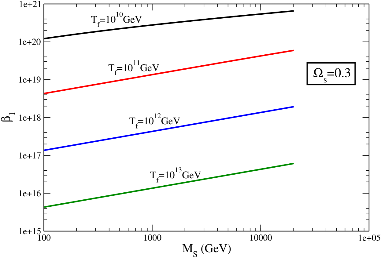
Figure 7: Coupling parameter $\beta_{1}$, as obtained by constraining the relic density of Weyl meson to be equal to the dark matter density($\Omega_{s}=0.3$) for different freeze out temperature $T_{f}$ and mass $M_{S}$.

The values of the parameter $\beta_{1}$ and $M_{S}$ for decoupling temperature $T_{f}=10^{10}$ to $10^{13}\,GeV$ are shown in Fig.7. We find, as expected, the lower $\beta_{1}$ leads to higher decoupling temperature. Hence for small value of coupling parameter Weyl meson get decoupled very early in the Universe. Furthermore $\beta_{1}$ also increase with $M_{S}$.

IV Decay Of Weyl Meson

In the previous section we have constrained the values of coupling parameters from the coannihilation rate and abundance of Weyl meson. But Weyl meson may also have the probability to decay into Higgs particles. So it may be possible that after the decoupling all the Weyl meson particles have already been decayed and today they may not be present in the Universe. In this section we calculate the decay rate of the Weyl meson and constraint its life time to be equal to the age of Universe. We show that the certain range of parameters $\beta_{1}$ and $M_{S}$ satisfiies these conditions.

We consider the simplest process for the decay of Weyl meson into pairs of Higgs particles and fermions, as shown in Fig.8

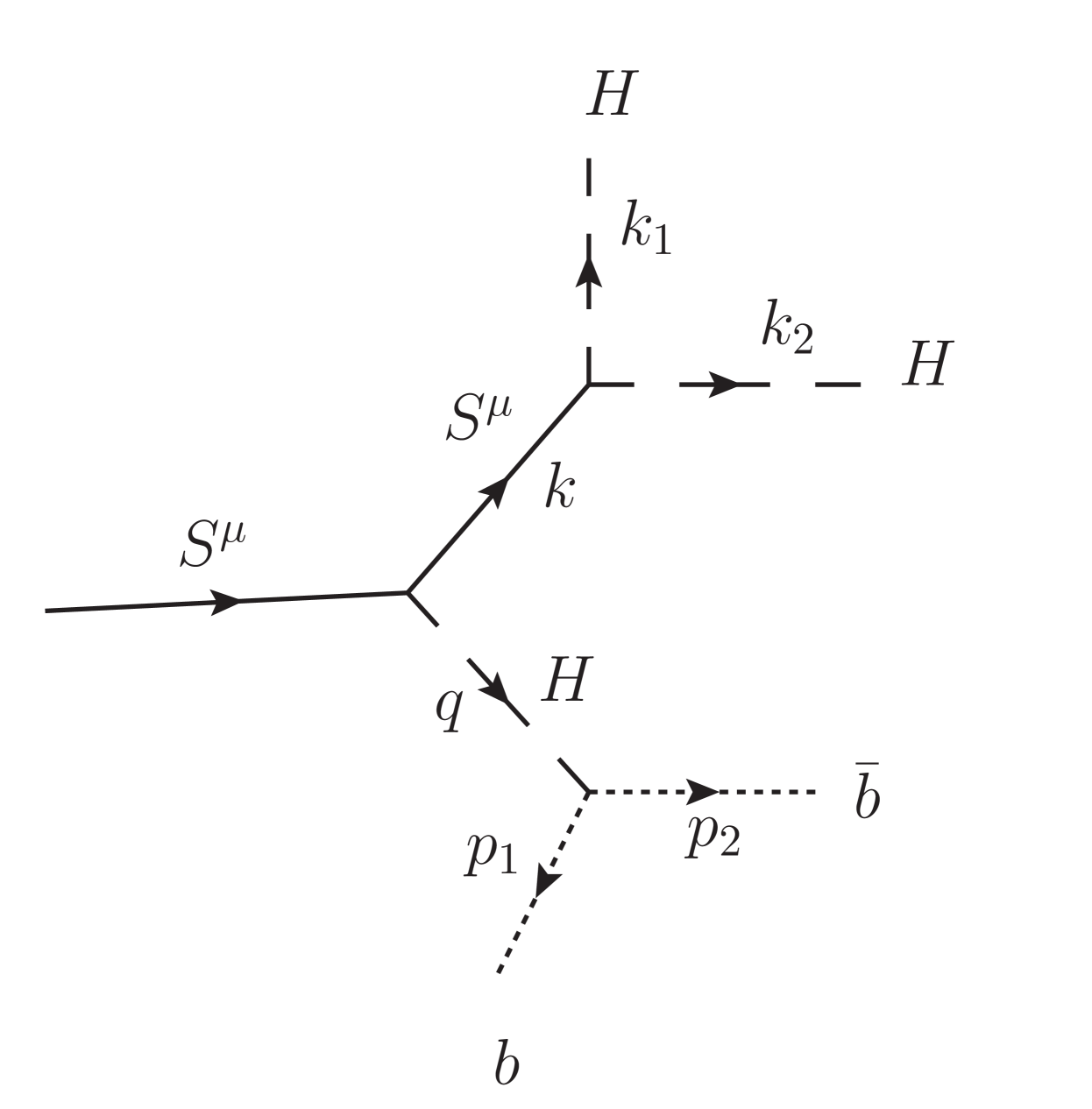
Figure 8: Decay process of Weyl meson.

The amplitude for this process is given by

$$\mathcal{M}= \frac{9}{8}f^{3}\beta_{1}^{2}\mathbf{v}(\sqrt{2}G_{f})^{\frac{1}{2}}m_{b}\frac{\epsilon^{\mu}k^{\nu}}{(k^{2}-m_{s}^{2})(q^{2}-m_{H}^{2})}$$

$$*\left(g_{\mu\nu}-\frac{k_{\mu}k_{\nu}}{m_{s}^{2}}\right)\bar{u}(p_{1})v(p_{2})$$ (50)

$$\sum_{spin}|{\mathcal{M}}|^{2}= \frac{A^{2}(f^{3}\beta_{1}^{2})^{2}(\epsilon.k)^{2}(1-k^{2})^{2}(4p_{1}.p_{2}-4m_{b}^{2})}{(k^{2}-m_{s}^{2})^{2}(q^{2}-m_{H}^{2})^{2}},$$ (51)

where $A$ contains all the constant. Now we define four momenta square $s_{12},s_{34}$, such that

$$k^{2}=(q_{1}+q_{2})^{2}=s_{12},\quad q^{2}=(p_{1}+p_{2})^{2}=s_{34}.$$ (52)

In term of these variables, we find

$$p_{1}.p_{2}=(\frac{s_{34}}{2}-m_{b}^{2}),\quad(\epsilon.k)^{2}=-s_{12}+\frac{m_{s}^{2}+s_{12}-s_{34}}{m_{s}^{2}}$$ (53)

and hence the amplitude of this process becomes function of the variables $s_{12}$ and $s_{34}$.
The decay rate for this process is

$$\Gamma=\frac{1}{2M_{S}}\int\sum_{spin}|{\mathcal{M}}|^{2}d\Phi,$$ (54)

where $d\Phi$ is the four dimensional phase space integral and again can be decomposed into product of two dimensional phase space integralhitoshi

$$\int d\Phi=\int\frac{ds_{12}}{2\pi}\frac{ds_{34}}{2\pi}d\Phi_{2}(\hat{p_{1}},\hat{p_{2}})d\Phi_{2}(\hat{q_{1}},\hat{q_{2}})d\Phi_{2}(\hat{q},\hat{k})$$

Here $d\Phi_{2}(\hat{p}_{i},\hat{p}_{j})$ is the two dimensional phase space integral in rest frame of particles having momentum $\hat{p}_{i}$ and $\hat{p}_{j}$.

If Weyl meson is a suitable dark matter candidate then it must be present in today’s Universe. So its life time($\tau=1/{\Gamma}$) must be at least equal to or greater than the age of the Universe. We determine $\Gamma$ numerically from Eq.(54) and find those values of $\beta_{1}$ and $M_{S}$ for which the life time of Weyl meson is equal to the age of the Universe $(\tau\approx 10^{42}GeV^{-1})$.

We have considered only the simplest process of the Weyl meson’s decay, as we are interested only in its decay rate to constrain the value of parameter $\beta_{1}$ and mass $M_{S}$. Final decay products can also be photons or electron-positron pairs. There are many observations showing the excess of positrons in cosmic rays pamela ; fermi . This excess of positrons may also be due to the decay products of the Weyl meson. We postpone the detailed analysis and fitting of the data for future research.

Now we have the posible range of parameter $\beta_{1}$ and mass $M_{S}$ from its relic density condition and its decay rate constraint. If Weyl meson is the dark matter candidate then it must satisfy both of these conditions. Combining these two results we have obtained the possible values of $\beta_{1}$ and $M_{S}$ for the Weyl meson, as shown in Fig.9.

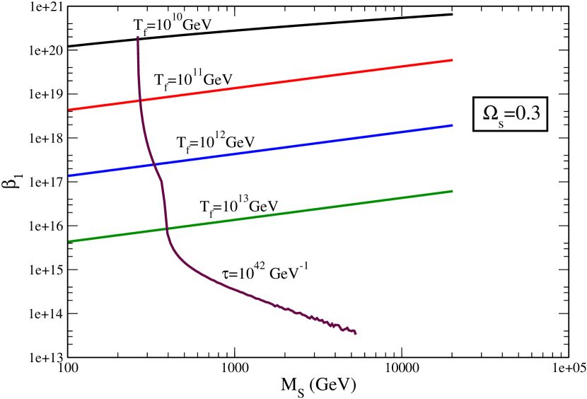
Figure 9: Possible values of parameter $\beta_{1}$ and mass $M_{S}$ of Weyl meson to solve the dark matter problem at given decoupling temperature $T_{f}$.

Here decoupling temperature $T_{f}$ is still an unknown parameter, but the intersting result which we have obtained is that the mass of the Weyl meson can not be greater than $500\,GeV$ and the parameter $\beta_{1}$ has minimum value $\approx 10^{15}$. These are the values which the Weyl meson can have if it is a very weakly interacting particle, such that it decouple immediately after the reheating of the Universe($T_{rh}\approx 10^{14}\,GeV$). If $\beta_{1}$ is smaller than $10^{15}$ then the Weyl meson decouples before the reheating of Universe and no constraint can be imposed on its relic density. We also find that the low mass range of the Weyl meson, which may be observable in colliders, is allowed by cosmological constraints.

V conclusion

Generalized locally scale invariant Standard Model leads to the direct coupling between the Weyl meson and the Higgs bosonquantumweyl . Weyl meson has been introduced in 1929 weyl . In this paper we have discussed the implications of the Weyl meson in collider physics and in cosmology in detail. We find that in the colliders real Weyl meson can not be produced for such type of interaction, but it can be produced virtually and leads to the production of three Higgs particles. We have discussed the three Higgs production process at LHC which can give us the signature of the Weyl meson for some finite value of coupling parameter. Furthermore, in this model Weyl meson acts as a dark matter candidate. We have discussed how for certain range of coupling parameter $\beta_{1}$ and mass $M_{S}$ Weyl meson can solve the dark matter problem. Although its decoupling temperature $T_{f}$ is still an unknown parameter, but we have found the upper bound for the Weyl meson mass $M_{S}$ and lower bound for its parameter $\beta_{1}$ ( $M_{S}<500\,GeV\;,\beta_{1}>10^{15})$ so that it is in thermal equillibrium with the cosmic fluid at some early time after the reheating of the Universe. In future we hope to have some data from colliders and from cosmic observations to test this model and to fix the values of these parameters.

References

- (1) J. H. Oort, Bull. Astron. Inst. Neth. 6, 249 (1932).
- (2) F. Zwicky, Helv. Phys. Acta. 6, 110 (1933).
- (3) F. Zwicky, Astrophys. J 86, 217 (1937).
- (4) V. Rubin and W. Ford, Astrophys. J 159, 379 (1970).
- (5) A. G. Riess et al., Astron. J. 116, 1009 (1998).
- (6) S. Perlmutter et al., Astrophys. J 517, 565 (1999).
- (7) E. Komatsu et al., Astrophys. J. Suppl. S. 192, 18 (2011).
- (8) G. Bertone, D. Hooper, and J. Silk, prep 405, 279 (2005).
- (9) G. Jungman, M. Kamionkowski, and K. Griest, Phys. Rep. 267, 195 (1996).
- (10) L. Bergstrom, Rep. Prog. Phys. 63, 793 (2000).
- (11) J. L. Feng, Annu. Rev. Astron. Astrophys. 48, 495 (2010).
- (12) G.Bertone, Particle Dark Matter: Observations, Models and Searches (Cambridge University Press, Cambridge, England, 2010).
- (13) H. Weyl, Z. Phys. 56, 330 (1929).
- (14) P. A. M. Dirac, Proc. R. Soc. A 333, 403 (1973).
- (15) D. K. Sen and K. A. Dunn, J. Math. Phys. 12, 578 (1971).
- (16) R. Utiyama, Prog. Theor. Phys. 50, 2080 (1973).
- (17) R. Utiyama, Prog. Theor. Phys. 53, 565 (1975).
- (18) P. G. Freund, Ann. Phys. 84, 440 (1974).
- (19) K. Hayashi, M. Kasuya, and T. Shirafuji, Prog. Theor. Phys. 57, 431 (1977).
- (20) K. Hayashi and T. Kugo, Prog. Theor. Phys. 61, 334 (1979).
- (21) M. Nishioka, Fortschr. Phys. 33, 241 (1985).
- (22) D. Ranganathan, J. Math. Phys. 28, 2437 (1987).
- (23) H. Nishino and S. Rajpoot, Phys. Rev. D 79, 125025 (2009).
- (24) H. Nishino and S. Rajpoot, Class. and Quant. Gr. 28, 145014 (2011)
- (25) P. Jain, S. Mitra, and N. K. Singh, J. Cosmol. Astropart. Phys. 2008, 011 (2008).
- (26) P.Jain and S.Mitra, Mod. Phys. Lett. A 22, 1651 (2007).
- (27) P.Jain and S.Mitra, Mod. Phys. Lett. A 25, 167 (2010).
- (28) H. Cheng, Phys. Rev. Lett 61, 2182 (1988).
- (29) H. Cheng, math-ph/0407010 (2004).
- (30) P.K.Aluri, P.Jain, and N.K.Singh, Mod. Phys. Lett. A 24, 1583 (2009).
- (31) H. Wei and R. G. Cai, J. Cosmol. Astropart. Phys. 2007, 015 (2007).
- (32) H. Wei and R. G. Cai, J. Cosmol. Astropart. Phys. 2007, 015 (2007).
- (33) S. D. Joglekar, Ann. Phys. 83, 427 (1974).
- (34) J. M. Cornwall, D. N. Levin, and G. Tiktopoulos, Phys. Rev. D 10, 1145 (1974).
- (35) N. K. Singh, P. Jain, S. Mitra, and S. Panda, Phys. Rev. D 84, 105037 (2011).
- (36) M. Shaposhnikov and D. Zenhäusern, Phys. Lett. B 671, 162 (2009).
- (37) J. F. Donoghue, Phys. Rev. D 50, 3874 (1994).
- (38) S.Dawson, hep-ph/9411325v1 (1994).
- (39) V. Barger and R. Phillips, Collider Physics, Frontiers in Physics (Addison-Wesley Pub. Co., New York, 1997).
- (40) T. P. Cheng and L. F. Li, Gauge Theory of elementary particle physics (Clarendon Press, Oxford, 1985).
- (41) S. Bentvelsen, E. Laenen, and P. Motylinski, NIKHEF, 2005-007.
- (42) F. Halzen and A. D.Martin, Quarks and Leptons: An Introductory Course in Modern Particle Physics (John Wiley and Sons, New York, 1984).
- (43) J. W. Williamson, Amm. J. Phys. 33, 987 (1965).
- (44) H. Murayama, Notes on Phase Space, Physics 233B, 2007.
- (45) P. Gondolo and G. Gelmini, Nucl. Phys. B 360, 145 (1991).
- (46) J. Edsjö and P. Gondolo, Phys. Rev. D 56, 1879 (1997).
- (47) M. Drees, M. Kakizaki, and S. Kulkarni, Phys. Rev. D 80, 043505 (2009).
- (48) E.W.Kolb and M.S.Turner, The Early Universe (Westview Press, Boulder, 1994).
- (49) O. Adrian et al., Nature 458, 607 (2009).
- (50) M. Ackerman et al., astro-ph.HE/1008.3999v2 .