The H₂O southern Galactic Plane Survey (HOPS): NH₃ (1,1) and (2,2) catalogues

Abstract

The H₂O Southern Galactic Plane Survey (HOPS) has mapped a 100 degree strip of the Galactic plane ($-70\mbox{${}^{\circ}$}>l>30\mbox{${}^{\circ}$}$, $|b|<0.5^{\circ}$) using the 22-m Mopra antenna at 12-mm wavelengths. Observations were conducted in on-the-fly mode using the Mopra spectrometer (MOPS), targeting water masers, thermal molecular emission and radio-recombination lines. Foremost among the thermal lines are the 23 GHz transitions of NH₃ J,K = (1,1) and (2,2), which trace the densest parts of molecular clouds ($n>10^{4}$ cm^-3). In this paper we present the NH₃ (1,1) and (2,2) data, which have a resolution of 2 arcmin and cover a velocity range of $\pm 200\,\mbox{km\,s${}^{-1}$}$. The median sensitivity of the NH₃ data-cubes is $\sigma_{T_{\rm mb}}=0.20\pm 0.06$ K. For the (1,1) transition this sensitivity equates to a 3.2 kpc distance limit for detecting a 20 K, 400 M_⊙ cloud at the 5$\sigma$ level. Similar clouds of mass 5,000 M_⊙ would be detected as far as the Galactic centre, while 30,000 M_⊙ clouds would be seen across the Galaxy. We have developed an automatic emission finding procedure based on the ATNF DUCHAMP software and have used it to create a new catalogue of 669 dense molecular clouds. The catalogue is 100 percent complete at the 5$\sigma$ detection limit ($T_{\rm mb}=1.0$ K). A preliminary analysis of the ensemble cloud properties suggest that the near kinematic distances are favoured. The cloud positions are consistent with current models of the Galaxy containing a long bar. Combined with other Galactic plane surveys this new molecular-line dataset constitutes a key tool for examining Galactic structure and evolution. Data-cubes, spectra and catalogues are available to the community via the HOPS website.

1 Introduction

HOPS (H₂O Southern Galactic Plane Survey) is a project utilising the Mopra radio telescope to simultaneously map spectral-line emission along the southern Galactic plane across the full 12-mm band (frequencies of 19.5 to 27.5 GHz). Since the survey began in 2007 (Walsh et al., 2008) HOPS has mapped 100 square degrees of the Galactic plane, from $l=290^{\circ}$, continuing through the Galactic centre to $l=30^{\circ}$ and with Galactic latitude $|b|\leq 0.5^{\circ}$. The aim of the survey is to provide an untargeted census of 22.235 GHz H₂O (6${}_{16}-$5₂₃) masers and thermal line emission towards the inner Galaxy. Observations were completed in 2010 and the survey properties, observing parameters, data reduction and H₂O maser catalogue are described in Walsh et al. (2011) (hereafter Paper I).

The primary thermal lines targeted by HOPS are those of ammonia (NH₃), whose utility as a molecular thermometer in a broad range of environments is unsurpassed. With an effective critical density of $\sim 10^{4}$ cm^-3 (Ho & Townes, 1983), NH₃ traces dense molecular gas and it is often associated with the hot molecular core phase of high-mass star formation (e.g., Longmore et al. 2007, Morgan et al. 2010), where it exhibits temperatures in excess of 30 K. NH₃ is excited in gas with kinetic temperatures greater than $\sim 5$ K (Pickett et al., 1998) and is also found associated with cool ($T<10$ K) dense clouds. Such regions are too cold for more common gas tracers, like CO, to remain in the gas phase. Instead they are frozen out onto the surfaces of dust grains (Bergin et al., 2006). The J,K = (1,1) inversion transition exhibits prominent hyperfine structure, which can be used to infer the optical depth of the transition. In clouds forming high-mass stars ($\geq 8\,\mbox{M${}_{\odot}$}$) and under optically thin conditions, the peak brightness of the four groups of satellite lines is approximately half that of the central group (Rydbeck et al., 1977). Comparison of the (1,1) and higher J,K inversion transitions can be used to estimate the rotational temperature of the gas.

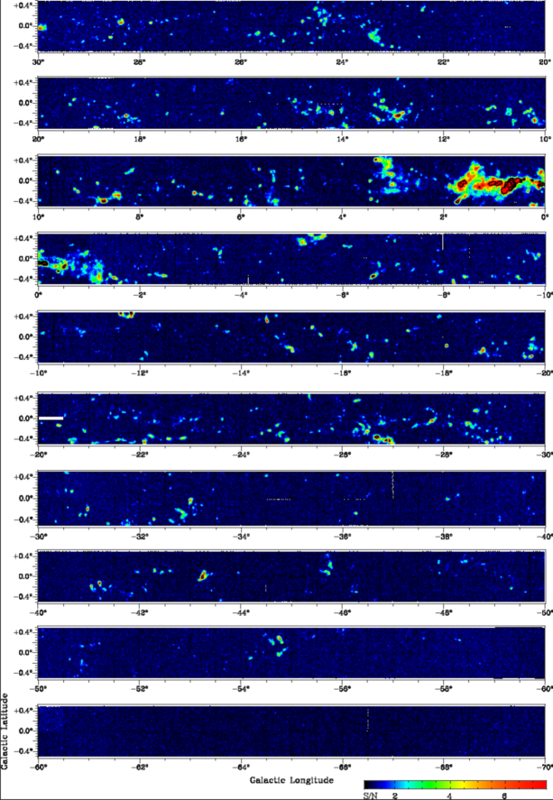
Figure 1: Map of the peak NH₃ (1,1) signal-to-noise (S/N) across the HOPS survey area. The map was made by smoothing the S/N cube spatially (final beam FWHM = 2.5 arcmin) and in velocity (hanning-window = 5) and measuring the peak brightness in each spectrum. An approximate brightness temperature scale may be found by multiplying by the average root-mean-squared noise temperature $\langle\sigma_{T_{\rm mb}}\rangle$ = 0.20 K.

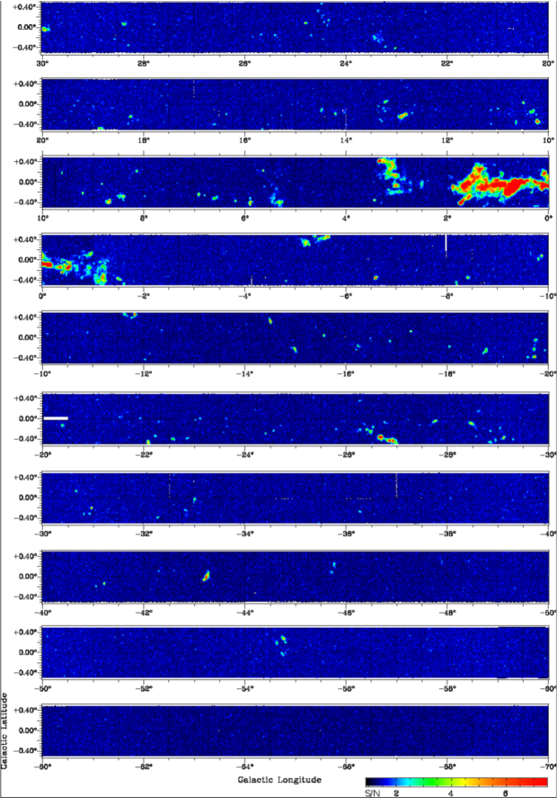
Figure 2: Map of the peak NH₃ (2,2) signal-to-noise (S/N) across the HOPS survey area.

In this second paper we present the HOPS NH₃ (1,1) and NH₃ (2,2) datasets and the automatic finding procedure used to create catalogues of emission. We illustrate the basic properties of the catalogues, which form the basis for further analysis. A third paper (Longmore et al. in prep.) will published the properties of the catalogue derived by fitting the NH₃ (1,1) and NH₃ (2,2) spectra with model line profiles (i.e. temperature, density, mass and evolutionary state).

2 Observations and data reduction

The HOPS observations and survey design are described in Walsh et al. (2008) and in Paper I. For convenience a brief summary is provided here.

2.1 Observations

Observations were conducted using the 22-m Mopra radio-telescope situated at latitude 31:16:04 south, longitude 149:05:58 east and at an elevation of 850 meters above sea level. Data were recorded over four summer seasons during the years 2007 – 2010 using a single-element 12-mm receiver.

The digitised signal from the receiver was fed into the Mopra Spectrometer (MOPS) backend, which has an 8.3 GHz total bandwidth split into four overlapping sub-bands, each 2.2 GHz wide. During the HOPS observations the spectrometer was configured in ‘zoom’ mode, whereby each of the sub-bands contained four 137.5 MHz zoom bands. Up to sixteen zoom bands may be recorded to disk, each split into 4096 channels. A single zoom band covered both the J,K = (1,1) and (2,2) NH₃ inversion transitions, which have line-centre rest frequencies of 23.6944803 GHz and 23.7226336 GHz, respectively (Pickett et al., 1998). This frequency setup resulted in a velocity resolution of $\sim 0.42\,\mbox{km\,s${}^{-1}$}$ per channel, spanning a velocity range of $1739\,\mbox{km\,s${}^{-1}$}$.

At 23.7 GHz the full-with half-maximum (FWHM) of the Mopra beam is 2.0 arcmin (Urquhart et al., 2010), meaning that the 100 square degree target area would require 90,000 pointings to create a fully sampled point-map. Based on experience gained during the pilot observations (Walsh et al., 2008) the survey area was divided up into 400 $0.5\mbox{${}^{\circ}$}\times 0.5\mbox{${}^{\circ}$}$ maps in Galactic coordinates. The telescope was driven in on-the-fly (OTF) mode, raster-scanning in either Galactic $l$ or $b$ and recording spectra every six seconds. At the end of each row spectra were taken of an emission-free reference position situated away from the Galactic plane. Scan rows were offset by half a beam FWHM and a scan rate was chosen to ensure Nyquist sampling at the highest frequency. Each map was observed twice by scanning in orthogonal $l$ and $b$ directions the results were averaged together to minimise observing artifacts.

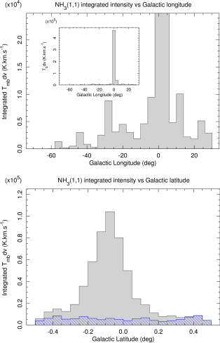
Figure 3: The top panel shows the sum of the NH₃ (1,1) integrated intensity over the survey region as a function of Galactic longitude in four-degree bins. The longitude bin covering the Central Molecular Zone (CMZ, $-2^{\circ}<\,l<2^{\circ}$) peaks at $\int T_{\rm mb}\,$dv = $4.65\times 10^{5}$ K $\mbox{km\,s${}^{-1}$}^{-1}$ and the y-axis scale has been truncated so as to show the remainder of the emission. The inset shows how the plot appears scaled to the full $\int T_{\rm mb}\,$dv range. In the bottom panel is a similar plot of $\int T_{\rm mb}\,$dv versus Galactic latitude. The filled grey histogram includes all emission, while the hatched histogram includes only emission outside the CMZ.

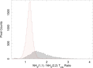
Figure 4: Plots of the brightness ratio $T_{\rm mb,\,(1,1)}/T_{\rm mb,\,(2,2)}$ for every emitting voxel ($l$-$b$-$v$ data element) with $T_{\rm mb}>3\sigma$ in both HOPS NH₃ datasets. The hatched histogram includes only voxels from the CMZ ($|l|<2\mbox{${}^{\circ}$}$) while the solid histogram includes the remaining emission from the outer Galaxy.

2.2 Data reduction

Raw data from the telescope were written into RPFITS format files consisting of lists of spectra with associated time-stamps and coordinate information. The ATNF LIVEDATA software package was used to apply a bandpass correction by forming a quotient between the reference spectrum and individual spectra in its associated scan row. The software was configured to fit and subtract a first order polynomial from the bandpass, excluding any strong lines and 150 noisy channels at each edge.

The GRIDZILLA package was used to resample the bandpass corrected spectra onto a regular coordinate grid. The software also performed interpolation in velocity space to convert measured topocentric frequency channels into LSR velocity. At this stage spectra with system temperatures $T_{\rm sys}>120$ K were discarded. Software settings were chosen to produce data cubes with pixel scales of $30\times 30$ arcsec and a resolution of 2 arcmin. The final data products were $1\times 10$ deg² cubes with 3896 usable velocity channels. For each spectral line within this pass-band the data has been cropped to $\pm\,200\,\mbox{km\,s${}^{-1}$}$ centred on the line centre velocity (determined from the line rest frequency), which corresponds to the normal velocity range for molecular material in the Galaxy (Dame et al., 2001).

A small number of spectra ($\sim 10$ percent) were affected by a baseline ripple or a depressed zero level. We fitted additional polynomial baselines of order 3 – 5 to the line-free channels of these data. See Appendix A for more detail.

2.3 Temperature scale and uncertainty

Data from Mopra are calibrated in brightness temperature units (K) on the $T_{\rm A}^{*}$ scale, i.e., they are corrected for radiative loss and rearward scattering (although not atmospheric attenuation at 12-mm wavelengths - see Kutner & Ulich 1981 for a review and also Ladd et al. 2005). It is desirable to convert this onto a telescope-independent main beam brightness temperature scale ($T_{\rm mb}$), which is also corrected for forward scattering. The measured $T_{\rm mb}$ of a source would equal the true brightness temperature if the source just filled the main beam. Urquhart et al. (2010) characterised the telescope efficiencies between 17 GHz and 49 GHz and we divided the HOPS data by the main-beam efficiency, $\eta_{\rm mb}$, given therein. For both NH₃ (1,1) and (2,2) data $\eta_{\rm mb}=0.571$. The uncertainty on the $T_{\rm mb}$ scale for HOPS is $\sim 30$ percent (Walsh et al., 2011).

3 The NH₃ data

In contrast to other large molecular line surveys of the Galactic plane, which use relatively abundant CO isotopologues (e.g. Dame et al. 2001, Jackson et al. 2006) HOPS has focused on the inversion-rotation transitions of NH₃. Detections derive from the densest parts of giant molecular clouds where gas is condensed into cool clumps, or in the case of warm gas ($T>30$ K) surrounding centrally heated star-forming regions (e.g., Purcell et al. 2009).

3.1 NH₃ emission properties

Figures 1 and 2 present peak signal-to-noise (S/N) maps covering the NH₃ (1,1) and (2,2) passbands, respectively ($|v_{\rm LSR}|<200\,\mbox{km\,s${}^{-1}$}$). Such maps are the easiest way to visualise the distribution of emission on the sky without becoming confused by noise-related artifacts. The maps were constructed by smoothing a S/N cube to a spatial resolution of 2.5 arcmin and then hanning-smoothing in the spectral dimension using a filter width of five channels ($\sim 2.0\,\mbox{km\,s${}^{-1}$}$). For any given spatial pixel the brightest spectral channel was recorded on the map. The S/N cube was generated during the emission-finding process, which is explained in Section 4.

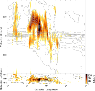
Figure 5: Detail of the longitude-velocity diagram showing the Galactic centre region (top). NH₃ (1,1) emission is shown in colourscale and the Dame et al. (2001) CO (1 – 0) contours are overplotted. While the overall emission morphology of both molecules is similar, the brightest peaks are offset in $l$ and $v$. The emission seen at $v<-170\,\mbox{km\,s${}^{-1}$}$ is due to broad linewidth NH₃ (2,2) emission encroaching on the NH₃ (1,1) pass-band. The bottom panel shows the NH₃ (1,1) integrated intensity map for the same $l$ range.

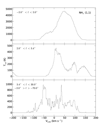
Figure 6: Integrated NH₃ (1,1) spectrum for the Galactic centre (top panel), the region around the G$3.34+0.42$ cloud, also known as Bania’s Clump 2 (middle panel), and the outer Galaxy (bottom panel). Spectra were integrated over the full latitude range ($\pm 0.5\mbox{${}^{\circ}$}$).

3.1.1 Galactic distribution of emission

The NH₃ (1,1) map (Figure 1) reveals a multitude of distinct clouds between $-30^{\circ}\,<l\,<\,30^{\circ}$. The density of clouds falls off rapidly in the southern Galaxy beyond $l<-30^{\circ}$. Several well known star-formation complexes are detected as bright peaks including G333.0-0.4 (Bains et al. 2006, Wong et al. 2008, Lo et al. 2009), W43 (G29.9, Dame et al. 1986, Nguyen Luong et al. 2011), G305 (Clark & Porter 2004, Hindson et al. 2010) and the ‘Nessie’ filament at $l=-21.5^{\circ}\,$, $b=-0.48\mbox{${}^{\circ}$}$ (Jackson et al., 2010). Emission from the Galactic centre region is most prominent between $-2^{\circ}\,<l\,<\,2^{\circ}$ and although symmetric in overall morphology, is significantly brighter at positive longitudes. Gas in this region, known in the literature as the Central Molecular Zone (CMZ), is characterised by high temperatures and densities, and by large velocity dispersions as it flows into the central 200 pc of the Galaxy (Morris & Serabyn, 1996).

Figure 3 illustrates the distribution of NH₃ (1,1) emission as histogram. The top panel shows the total integrated intensity (summed over all $v$ and $b$) as a function of Galactic longitude in 4^∘ bins. The CMZ contains 80.6 percent of the detected NH₃ (1,1) emission and dominates the plot, which is scaled to show the less intense emission in the outer Galaxy. The bottom panel shows the same plot as a function of Galactic latitude in 3 arcmin bins. The filled grey histogram incorporates all emission in the HOPS target region. The broad and intense peak at $b=-0.075\mbox{${}^{\circ}$}$ is solely due to emission from the CMZ. However, with the Galactic centre removed (hatched histogram), the distribution with $b$ is relatively flat.

It is interesting to note that the Galactic distribution of H₂O masers found in HOPS (Walsh et al., 2011) is very different to that of the dense molecular gas traced by NH₃. The masers show no evidence of a longitude peak at the Galactic centre, but are clustered around the mid-plane of the Galactic disk with an angular scale-height of $\theta_{\rm FWHM}=0.60^{\circ}$. The implications for star-forming environments in the CMZ compared to the spiral arms will be discussed in a future paper (Longmore et al., in prep).

3.1.2 NH₃ (1,1) versus NH₃ (2,2) emission

Only one-third of the NH₃ (1,1) emission regions detected above 3$\sigma$ have counterparts in the NH₃ (2,2) data, despite the data having similar sensitivities. Most clouds with $T_{\rm mb,\,(1,1)}>$1 K are detected in the (2,2) data, although there are exceptions (for example the cloud at $l=-2.5\mbox{${}^{\circ}$},b=0.33\mbox{${}^{\circ}$}$). Where emission is detected in both lines, the brightness ratio $T_{\rm mb,\,(1,1)}/T_{\rm mb,\,(2,2)}$ varies between $\sim 0.2$ and $\sim 4.2$ over the HOPS area. Clouds with low ratios or no detected NH₃ (2,2) emission tend to be associated with extinction features in the GLIMPSE $8\,\micron$ infrared images and are excellent candidates for the cold and dense precursors to clusters of high-mass stars. Strikingly, the morphology of the CMZ is almost identical in both datasets and the brightness-temperature ratio is uniformly close to one. Figure 4 illustrates this difference graphically by plotting the distribution of brightness-temperature ratios between every common emitting voxel (3-dimensional data elements in $l$, $b$ & $v$) with $T_{\rm mb}>3\sigma$. The tall, narrow histogram (hatched) contains voxels drawn from the CMZ only and has a median of 1.2 and a width of $\sigma=0.19$. By comparison the data from the outer Galaxy has a median of 1.6 and $\sigma=0.50$. Lower ratios in the CMZ are consistent with warmer excitation conditions, but may also be due in part to the effects of high optical depths or line saturation.

A small proportion of NH₃ (2,2) emission is not associated with NH₃ (1,1) emission at the same location. The J,K = (1,1) transition is more easily excited than the (2,2), hence such NH₃ (2,2) detections are most likely artifacts. We analyse the completeness and spurious source counts in Sections 5 and 5.3.

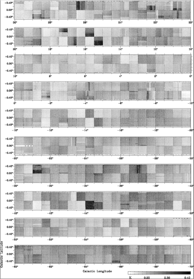
Figure 7: Image of the root-mean-squared noise temperature in $T_{\rm mb}$ units for the entire HOPS region made from the NH₃ (1,1) data. Individual observing blocks are visible as 0.5^∘ chequered squares, while scanning artifacts present as lines of high or low noise in Galactic $l$ and $b$. The median root-mean-squared noise is 0.20 K $\pm$ 0.05 K, where the uncertainty is the FWHM of the total noise distribution (also see Figure 8.

3.1.3 Position-velocity Diagram

Spectral lines originating from the Galactic centre region have extremely broad profiles ($>50\,\mbox{km\,s${}^{-1}$}$) and merge together into a single bright region of emission with a complex morphology. Figure 5 (top) is an $l$-$v$ diagram showing the inner eight degrees of the Galactic plane and the prominent CMZ. To make the map, voxels without detected emission were set to zero and the data were summed in Galactic latitude. The corresponding integrated intensity map is presented in the bottom panel. A significant velocity gradient exists across the emission, which has also been observed in the Dame et al. (2001) CO (1 – 0) data. Rodriguez-Fernandez & Combes (2008) have modelled the CMZ as the gas response to a short ‘nuclear bar’, which itself is embedded within a longer Galactic bar, thought to be inclined towards us at an angle of $25\mbox{${}^{\circ}$}\,-\,35\mbox{${}^{\circ}$}$, with the nearer end at positive Galactic longitudes. The large broad-line region of emission at $l=3.1\mbox{${}^{\circ}$}$ is known as Bania’s Clump 2 (Bania, 1977) and has been theorised to lie at the closest end of innermost elongated x-1 orbit around the Galactic centre (Bally et al., 2010). The CO (1 – 0) contours from the 12 arcmin resolution Dame et al. (2001) survey are overlaid on the $l$-$v$ diagram for comparison. The overall morphology of the emission is similar, however, the 2 arcmin resolution NH₃ data shows more structure, both spatially and spectrally. Galactic CO (1 – 0) emission is optically thick compared to NH₃, which probes the kinematics of the molecular clouds at greater depths. NH₃ detections in HOPS are severely distance limited (see Section 5.3.3) and detecting emission from beyond the Galactic centre is difficult, even in the highly excited central Galaxy.

3.1.4 Integrated spectrum

The NH₃ (1,1) spectrum is characterised by five groups of emission lines seperated $\sim 10\,\mbox{km\,s${}^{-1}$}$. Under optically thin conditions the central group is approximately twice the brightness of the satellites. Figure 6 presents NH₃ (1,1) spectra summed over all $b$ and selected $l$ ranges. In the top panel is shown the integrated spectrum of the CMZ between $-2\mbox{${}^{\circ}$}<l<2\mbox{${}^{\circ}$}$. Individual spectra (and line-groups within spectra) are blended into a single emission feature spanning $-160\,\mbox{km\,s${}^{-1}$}<v_{\rm LSR}<160\,\mbox{km\,s${}^{-1}$}$. The middle panel shows the integrated spectrum of the region dominated by Bania’s clump 2 (G$3.34+0.42$ in this work), which has the broadest linewidths outside of the CMZ. Emission at $v_{\rm LSR}<-170\,\mbox{km\,s${}^{-1}$}$ is due to broad NH₃ (2,2) lines impinging on the NH₃ (1,1) bandpass. The spectrum in the bottom panel is constructed from the outer Galaxy data only and contains multiple distinct velocity features deriving from individual regions of emission. The peaks at approximately $-50\,\mbox{km\,s${}^{-1}$}$ and $+40\,\mbox{km\,s${}^{-1}$}$ are likely associated with the Galactic ring and Scutum-Centarus spiral arm, respectively (see Section 6.2). Some of the complexity evident in the ensemble spectrum may also be attributed to the summation of satellite line-groups.

3.2 Noise characteristics

Figure 7 shows an image of the root-mean-squared (RMS) noise temperature $\sigma_{T_{\rm mb}}$ over the whole survey region. The image was constructed by measuring the RMS noise along the spectral dimension of the NH₃ (1,1) cube after masking off all channels containing line-emission. We are confident that the noise map does not contain any contribution from real emission as contamination from the broad-linewidth CMZ is absent, and this represents the worst-case scenario.

The defining feature of Figure 7 is the chequered pattern corresponding to individual $0.5\times 0.5$ degree maps. The variable noise level between maps is due to temporal changes in the conditions encountered while observing. Within each map, rapidly fluctuating cloud cover and flagged or missing spectra lead to high-noise ‘hot-spots’. More gradual changes in observing conditions (e.g., humidity and elevation) manifest themselves as significant noise variations between scan-rows in $l$ or $b$. Automatically finding line-emission in such an inhomogeneous data-cube poses a distinct challenge.

Histogram plots of the noise temperature $\sigma_{T_{\rm mb}}$ for all spatial pixels in the HOPS NH₃ (1,1) and (2,2) data are plotted in Figure 8. Both datasets have Gaussian shaped distributions, except for a small number of pixels which occupy a tail extending to higher noise temperatures (0.71 % above 3$\sigma$). The median noise temperature of the J,K = (1,1) data is higher than the (2,2): $\sigma_{T_{\rm mb\,\,(1,1)}}=0.201$ K compared to $\sigma_{T_{\rm mb,\,(2,2)}}=0.186$ K, although the Gaussian part of both distributions have similar widths at FWHM${}_{(1,1)}=0.056$ K and FWHM${}_{(2,2)}=0.053$ K. Upon inspection of the data we find that the high-noise pixels in the tail arise from $\sim 10\mbox{${}^{\circ}$}$ maps observed during poor weather and from the edges of the maps where fewer raw spectra contribute to individual pixels. The difference between the NH₃ (1,1) and (2,2) distributions stems from a single low-noise NH₃ (2,2) map which had additional data added into the processing pipeline. No emission was detected in this map, which lies in the far southern Galactic plane at $l=-60.25$, $b=0.25$.

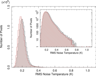
Figure 8: Histograms of the RMS noise temperature for all $(l,b)$ spatial pixels in the NH₃ (1,1) and (2,2) data (grey-shaded and hatched histograms, respectively). The noise temperatures were determined from the line-free channels in the spectra. Inset is the same histogram, but with a logarithmic scaling on the Y-axis to enhance the view of the high-noise tail.

4 Source finding and measurement

The full HOPS dataset covers 100 square degrees of the sky, equivalent to over 90,000 overlapping Gaussian beams at 23.7 GHz. For each position we obtain a spectrum spanning a 400 km s^-1 velocity range, or 931 channels. Manually identifying emission in such a large volume of data would be prohibitively tedious and likely error-prone, so an automatic emission finding procedure was written for HOPS. At the core of the method is the ATNF’s duchamp software (Whiting, 2012), which has been developed to automatically detect emission in three-dimensional data. duchamp is specifically designed for the case of a small number of signal voxels within a large amount of noise and is perfectly suited to the wide bandwidth data-cubes produced by the Mopra spectrometer.

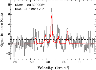
Figure 9: Example signal-to-noise spectrum (grey line) extracted from a single pixel with the wavelet-reconstructed spectrum overlaid (red-line). Duchamp does an excellent job of suppressing the noise allowing the use of a low threshold: 0.8$\sigma$ in this case.

4.1 Overview of the source finding procedure

duchamp searches a cube by applying a single threshold, either a flux value or a signal-to-noise ratio, for the whole dataset, and so is thus best applied to data with uniform noise. To compensate for the variable noise in the NH₃ data, the HOPS emission finding procedure implements a two-pass solution. Firstly duchamp is run on a smoothed version of the entire cube down to a global 3$\sigma$ cutoff level. A mask data-cube is produced which is used to blank the emission in the original data. Some of this ‘emission’ identified in the first pass may in fact be regions of high RMS noise and conversely some real low-level emission may have escaped detection. However, this likely does not matter as the goal of this step is to create a cube containing mostly line-free noise. For every spatial pixel in the blanked cube the standard deviation ($\sigma_{T_{\rm mb}}$) is estimated along the spectral axis to create a map of background noise temperature like that shown in Figure 7. In practice we calculate the median absolute deviation from the median (MADFM), which for a dataset X = x₁, x₂ … x_i… x_n is given by:

$${\rm\sigma=K.median\,(|x_{i}-median(X)|)},$$ (1)

i.e., the median of the deviations from the median value. In Equation 1, K is a constant scale factor which depends on the distribution. For normally distributed data K $\approx$ 1.48. The MADFM statistic is largely robust to the presence of a few channels much brighter than the noise. This is especially important when estimating the noise in spectra containing very broad lines, such as those observed towards the Galactic centre.

Each spectral plane of the original input cube is then divided by the noise map to make a signal-to-noise cube with homogeneous noise properties. duchamp offers the option of reconstructing data-cubes using the à trous wavelet method prior to running the finder. A thorough description of the procedure may be found in Starck & Murtagh (1994). The reconstruction is very effective at suppressing noise in the cube, allowing the user to search reliably to fainter levels and reducing the number of spurious detections. We chose to reconstruct the NH₃ data in 3D-mode, meaning that the wavelet filters can distinguish between narrow noise spikes confined to single channels and small regions of emission spanning $l$-$b$-$v$ space. Figure 9 shows an example NH₃ (1,1) spectrum with the reconstructed version overplotted. A second pass of duchamp is run on the reconstructed cube to construct the final list of emission sources. A detailed description of the duchamp inputs is presented in Appendix B.

4.2 Cloud measurements

The properties of NH₃ clouds were measured directly from the NH₃ data cubes using the 3D voxel-based emission masks produced by the source finder. Two dimensional pixel-masks were made by collapsing the 3D masks along the velocity axis.

4.2.1 Position, velocity and angular size

Three position and velocity measurements were made on each cloud: centroid, weighted and peak. The centroid position ($l_{\rm c},\,b_{\rm c},\,v_{\rm c}$) was measured directly from the 3D voxel mask and corresponds to the geometric centre of the cloud in $l$-$b$-$v$ space. A brightness weighted position ($l_{\rm w},\,b_{\rm w},\,v_{\rm w}$) was measured by weighting each voxel coordinate with its brightness temperature value $T_{\rm mb}$ according to:

$$n_{\rm w}=\left.\displaystyle\sum\limits_{i=1}^{n}\,n_{i}~{}T_{{\rm mb},i}\middle/\displaystyle\sum\limits_{i=1}^{n}T_{{\rm mb},i},\right.$$ (2)

where $n$ is the coordinate axis to be measured. The peak position ($l_{\rm p},\,b_{\rm p},\,v_{\rm p}$) is the coordinate of the brightest voxel in the 3D cloud. Noise spikes can introduce significant errors in the weighted and peak measurements, especially for weak detections, so we performed the coordinate measurements on cubes spatially smoothed to a resolution of 2.5 arcmin and spectrally smoothed using a hanning window five channels wide. Sources with simple morphologies have similar positions and velocities in all three measurements compared to extended sources in which the measurements differ.

4.2.2 Angular size and area

The angular size of the clouds was quantified in two ways. Firstly, the solid angle $\Omega$ subtended by the cloud was measured from the 2D pixel mask. The equivalent angular radius $r_{c}$ is then defined as the radius of a circular source which would subtend an equivalent solid angle on the sky. Secondly, the brightness-weighted radius $r_{\rm w}$ was calculated with respect to the ($l_{\rm w},\,b_{\rm w}$) position via:

$$r_{\rm w}=\left.\displaystyle\sum\limits_{i=1}^{n}\,r_{i}~{}T_{{\rm mb},i}\middle/\displaystyle\sum\limits_{i=1}^{n}T_{{\rm mb},i},\right.$$ (3)

where $r_{i}$ is the distance between the brightness-weighted centre and the $i^{\rm th}$ pixel. For a high signal-to-noise ratio unresolved source this is directly equivalent to the Gaussian FWHM/2.

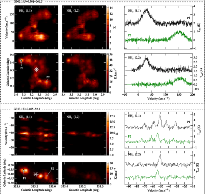
Figure 10: Examples of two bright clouds in HOPS. For each cloud we show the NH₃ (1,1) and (2,2) integrated intensity maps (bottom-left and bottom-middle panels, respectively), summed longitude velocity ($l$-$v$) diagrams (top-left and top-middle panels) and sample spectra from two local peak positions (right panels). The $l$-$v$ diagrams were made by summing over the Galactic $b$ axis of the cubes. The position of the brightest voxel is marked by a star symbol, the geometric centre by a ‘$+$’ and the brightness-weighted centre by a ‘$\times$’. See section 4.3 for details.

4.2.3 Integrated intensity and brightness temperature

The integrated intensity $\int T_{\rm mb}\,dv$ of a cloud is the summed brightness of the emitting voxels (in K) times the velocity-width $\Delta v$ of a channel (in km s^-1). We have an excellent measurement of the average RMS noise over the cloud (see Figure 7), so the uncertainty on $\int T_{\rm mb}\,dv$ is given by:

$$\delta\left(\int T_{\rm mb}\,dv\right)~{}=~{}\langle RMS\rangle\Delta v\,\sqrt{N},$$ (4)

where $N$ is the number of independent spatial pixels subtended by the cloud. Systematic fluctuations in the spectral baselines may also contribute to the error, but these are likely insignificant compared to the HOPS sensitivity.

The peak brightness temperature $T_{\rm mb}$ is simply the value of the brightest voxel in the cloud.

4.3 Example clouds

Forty-four percent of NH₃ (1,1) clouds in HOPS are unresolved ($r_{\rm w}<1$ arcmin). Figure 10 presents examples of two bright and extended clouds. Both clouds show evidence of sub-structure in position and velocity, but are merged into a single object by the emission finder. G003.145+0301+066.5 (named for $l_{\rm c}$+$b_{\rm c}$+$v_{\rm c}$), also known as Bania’s Clump 2, (Bania, 1977), is interesting as it is one of the few clouds outside of the CMZ to exhibit very broad line profiles ($\delta v>50\,\mbox{km\,s${}^{-1}$}$). The emission is largely confined to two lobes separated in $b$ and $v$, but with components which merge at $v\approx 75$ km s^-1. Physical conditions in G003.145+0301+066.5 are comparable to the CMZ, as the median brightness ratio $T_{\rm mb,\,(1,1)}/T_{\rm mb,\,(2,2)}=1.2$ compared to 1.6 for clouds in the outer Galaxy.

G333.183$-$0.405$-$52 is a well known giant molecular cloud containing HII regions, hot molecular cores and outflow sources (see Lo et al. 2009 and references therein). In contrast to Bania’s Clump 2, the line profiles are well-defined. NH₃ (1,1) exhibits the classic spectral shape at both sampled positions: a central main group of lines with four symmetric satellite groups, approximately half as bright as the main-group. The spectrum of NH₃ (2,2) also exhibits four groups of satellite lines (see Pickett et al. 1998), but they are generally too weak to be detected in the HOPS data.

Overlaid on the $\int T_{\rm mb}dv$ maps are the three position measurements as described in Section 4.2. The peak voxel is denoted by a star, the geometric centre is marked by a ‘$+$’ and the brightness-weighted centre by a ‘$\times$’ symbol. Note that the peak voxel is not necessarily coincident with the peak pixel of the $\int T_{\rm mb}dv$ map. Geometric and brightness-weighted positions are generally in close agreement, even in clouds with complex morphology. Indeed, separations of more than a beam-width between these two positions and the peak voxel position indicates that multiple clumps of emission exist within a cloud boundary. The weighted method is the most robust, so we adopt the weight values from now on we when referring to longitude, latitude and $v_{\rm LSR}$ of a source.

5 The HOPS NH₃ catalogue

The emission finder was run on the NH₃ (1,1) and (2,2) datasets independently to produce the final catalogues of clouds. In total 669 NH₃ (1,1) and 248 NH₃ (2,2) clouds were found in the HOPS cubes. In the following sections we examine the catalogues produced by the source finding routines. We aim to quantify the robustness of the DUCHAMP detections and investigate the distribution of source properties.

5.1 NH₃ (1,1) versus (2,2) catalogues

The initial NH₃ (1,1) catalogue contained 687 detections of which 18 were flagged as artifacts. Five detections between $-2<l<2$ with $v_{\rm LSR}<-190\,\mbox{km\,s${}^{-1}$}$ are in fact bright, extended clouds of emission from the NH₃ (2,2) transition. The extremely large linewidths close to the Galactic centre ($50\,\mbox{km\,s${}^{-1}$}<\Delta v<100\,\mbox{km\,s${}^{-1}$}$) cause NH₃ (2,2) emission to spill over into the NH₃ (1,1) bandpass. A further thirteen detections are flagged as they arise from artifacts caused by the baselining routine. Due to the polynomial used to fit the baseline (see Appendix A), the spectra at the edge of the bandpass can rise slightly above the noise cutoff for several contiguous velocity channels. If this occurs for enough contiguous spatial pixels to pass the detection threshold the emission will be classed as a source. However, such sources are easy to flag by eye.

Duchamp originally found 324 individual clumps within the NH₃ (2,2) data-cube of which 76 are flagged as artifacts. Eighteen spurious detections are due to a turned-up bandpass-edge, or an intrusion by a broad NH₃ (1,1) linewing. The J,K = (1,1) transition is more easily excited than the (2,2), hence NH₃ (2,2) clouds are only considered valid if associated with (1,1) emission at the same position. Fifty-eight low level NH₃ (2,2) detections ($T_{\rm mb}<5\sigma$, $n_{\rm pixels}\leq 12$) were flagged as spurious for this reason. In Section 5.3, below, we investigate the formal catalogue completeness and contamination by spurious sources.

5.2 Catalogue description

Tables 2 and 3 present a sample of the catalogue entries for the NH₃ (1,1) and (2,2) data, respectively. The complete catalogue is available in electronic format on the HOPS website. Columns in the tables are as follows: (1) the cloud name constructed from the centroid position of the cloud in Galactic longitude, latitude and velocity; (2) the brightness-weighted Galactic longitude, (3) latitude and (4) $v_{\rm LSR}$ measured from a masked and smoothed version of the original cube. Columns (5), (6) and (7) contain the Galactic coordinates ($l$ & $b$) and velocity ($v_{\rm LSR}$) of the brightest voxel in the cloud. Columns (8) and (9) tabulate the velocity range over which DUCHAMP detects emission within that clump; column (10) contains the angular radius, in arcminutes, of a circular source subtending an equivalent solid angle on the sky and column (11) the brightness-weighted radius measured from the integrated intensity map. Column (12) contains the solid angle subtended by the cloud in square arcminutes; (13) the number of spatial pixels in the cloud; (14) the number of emitting voxels in the cloud, and (15) presents the total integrated intensity $\int$T${}_{\rm mb}dv$. The peak brightness temperature is recorded in (16) and the local RMS noise temperature in (17). Column (18) contains flags noting if the cloud touches a survey boundary in $b$ (=X), $l$ (=Y) or $v$ (=Z). The cloud is flagged with an ‘M’ if multiple velocity components were detected, i.e., if the velocity range is greater than the expected velocity width of a single NH₃ spectrum. Here we assume a FWHM for each line-group of $3\,\mbox{km\,s${}^{-1}$}$, which is typical of gas forming massive stars. The expected velocity range of an NH₃ (1,1) spectrum from an isolated cloud is then $44.6\,\mbox{km\,s${}^{-1}$}$. Clouds which exhibit significantly different peak and brightness-weighted velocities ($>5\,\mbox{km\,s${}^{-1}$}$) are likely to contain multiple sub-clouds overlapping in position and are flagged with an ‘E’. A small number of clouds detected in the NH₃ (1,1) bandpass are in fact broad line-wings of NH₃ (2,2) encroaching on the (1,1) bandpass and are flagged as artifacts with an ‘A’ in column 18. Similar artifacts in the (2,2) data are also marked with an ‘A’ in column 18.

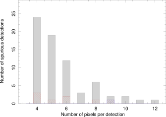
Figure 11: Histogram of the number of spurious sources detected in an ‘empty’ NH₃ (2,2) data cube (see Section 5.3.1 for details). The source finder was run at a range of sigma-limits to characterise the number of detections as a function of source solid angle. Grey bars = 0.7$\sigma$, red-hatched (left-slanted) bars = 0.8$\sigma$ and blue-hatched (right-slanted) bars = 0.9$\sigma$. Based on this plot a brightness cutoff of 0.8$\sigma$ was selected and a minimum of seven spatial pixels was required in a valid detection. The artificially low $\sigma$-limit is possible because the à trous reconstruction effectively suppresses most of the noise.

5.3 Catalogue completeness

5.3.1 Spurious sources

Although the data have been corrected for large scale inhomogeneities in the noise properties by fitting polynomial baselines (see Section 2.2 and Appendix A), higher order fluctuations are still present and masquerade as real emission near the sensitivity limits. To constrain the number of spurious sources as a function of cloud size and sensitivity we ran the source finder on an ‘empty’ test cube at a range of sigma limits. The test region was drawn from the NH₃ (2,2) dataset in the outer Galaxy (299.96^∘$\,>l>\,$292.54^∘, $|b|<\,$0.456^∘) and contains no believable molecular emission: i.e., when the source-finder is run at a very low level on both the NH₃ (1,1) and (2,2) data, none of the detected emission is common to the two datasets. We would expect the J,K = (1,1) and (2,2) transitions to arise in the same gas and the NH₃ (2,2) line to be weaker, hence, the detected (2,2) emission without corresponding (1,1) emission is likely spurious.

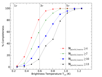
Figure 12: This figure shows the percentage completeness as a function of peak brightness temperature. The four curves illustrate the effect of varying the minimum number of spatial pixels required in a detection.

Figure 11 shows the number of spurious sources detected as a function of pixel count and sensitivity limit. Decreasing both the sensitivity and pixel limits has the effect of increasing the number of spurious sources found. In particular, dropping the sigma-limit from 0.8$\sigma$ to 0.7$\sigma$ results in an sharp increase from eight to seventy spurious detections. The 0.7$\sigma$ results also show that decreasing the minimum size of the clouds significantly increases the number of spurious detections. Based on these results we chose a sensitivity limit of 0.8$\sigma$ when source finding and required a minimum of seven spatial pixels in a valid detection.

Data in the test cube is of particularly high quality compared to the remainder of the survey and may not be wholly representative of all HOPS data (see Figure 7). Fifty-eight spurious $\mbox{NH${}_{3}$}\,(2,2)$ sources (i.e., without associated $\mbox{NH${}_{3}$}\,(1,1)$) were detected in the full survey, implying that significant numbers of spurious sources exist in the catalogues. However, most of these detections have signal-to-noise ratios below five and subtend less than twelve pixels on the sky. More conservative constraints may be imposed when defining a high-reliability catalogue, e.g., a cutoff of 13 pixels per source would provide a reasonable ‘safety margin’ for data where the noise properties are worse than in the test region. Applying such a cutoff to the $\mbox{NH${}_{3}$}\,(1,1)$ and (2,2) catalogues yields source counts of 523 and 198, respectively - a reduction of $\sim 20$ percent.

5.3.2 Completeness curves

We have estimated the completeness limits of the catalogue by injecting artificial point sources into the NH₃ (1,1) data and attempting to recover them using our DUCHAMP procedure. The region of Galactic plane from $l$ = 292.4^∘ to $l$ = 297.7^∘ is devoid of significant emission and was used as an input. During the experiment the FWHM Gaussian linewidth of the injected sources was set uniformly to 3 km s^-1, typical of high-mass star-forming clouds. The distribution of peak brightness temperatures ranged from 0.2 K to 1.3 K, spanning the expected sensitivity limits. One-hundred 3D Gaussian sources were inserted into the cube at random, non-overlapping positions, and the emission finding procedure was called to find them. After thirty iterations the positions of the clouds found by DUCHAMP were matched with the injected positions and the recovered sources divided into brightness bins. Figure 12 plots the percentage of sources recovered as a function of peak brightness. Apart from the obvious sensitivity limit, the limiting parameter on the number of clouds found is the number of pixels allowed within a valid detection. The figure shows curves for N${}_{\rm pixels}\,\geq\,4$, 7, 10 and 13 pixels with the 1$\sigma$, 3$\sigma$ and 5$\sigma$ sensitivity limits overplotted. When creating the HOPS NH₃ cloud catalogue we imposed a limit of $\geq 7$ pixels per valid detection, resulting in a 60 percent completeness level at 3$\sigma$ ($T_{\rm mb}=0.6$ K). The catalogue is 100 percent complete at the 5$\sigma$ level ($T_{\rm mb}=1.0$ K).

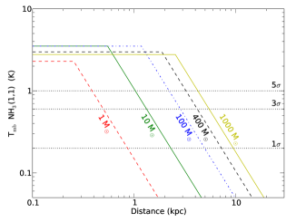
Figure 13: Plot of expected main-line brightness temperature versus distance for the five objects in Table 1. The one, three and five sigma sensitivity limits are plotted as horizontal dashed lines. For the parameters outlined in Table 1 we should detect a 10 M_⊙ cloud out to a distance of $\sim$ 1.0 kpc, and a 400 M_⊙ cloud out to 3.2 kpc at the $5\sigma$ level. The turnover occurs as a result of beam dilution: once the source is far enough away it no longer fills the main beam.

5.3.3 Completeness illustration

Table 1: Properties of the objects used to illustrate the survey completeness. The five objects are taken to be representative of an isolated low-mass core and low, intermediate and two high-mass star formation regions. A constant NH₃/H₂ abundance of 10^-8 was assumed. $T^{11}_{\rm ex}$, $T^{11}_{\rm mb}$ and $\tau$ were calculated using RADEX, as described in Section 5.3.3.

Mass	Radius	Density	$T_{\rm K}$	$\Delta V^{11}$	$T^{11}_{\rm ex}$	$T^{11}_{\rm mb}$	$\tau$
(M⊙)	(pc)	(cm-3)	(K)	(km s-1)	(K)	(K)
1	0.07	104	10	0.3	6.0	2.3	1.2
10	0.16	104	10	0.3	6.6	3.5	2.3
100	0.34	104	20	1.0	8.1	3.5	1.1
400	0.55	104	20	2.0	7.8	3.0	0.9
1000	0.74	104	20	3.0	7.7	2.8	0.8

To illustrate the completeness limits, we calculated the expected NH₃ (1,1) brightness temperature as a function of distance for five objects taken to be representative of an isolated low-mass core and low, intermediate and two high-mass star-forming regions. Starting with spherical clouds of a given mass and uniform density, we calculated the expected physical radius, projected angular size and NH₃ column density (from the H₂ column density assuming an H₂/NH₃ abundance). The radiation temperature $T_{\rm R}$, excitation temperature $T_{\rm ex}$ and optical depth $\tau$ of the NH₃ (1,1) line was then calculated using the RADEX radiative transfer package (van der Tak et al., 2007). RADEX is a one-dimensional non-LTE code that takes as input the kinetic temperature $T_{\rm kin}$, H₂ density, NH₃ column density and NH₃ linewidth. For each molecular transition it returns values for $T_{\rm R}$, $T_{\rm ex}$ and $\tau$. The measured main-beam brightness temperature $T_{\rm mb}$ was calculated from $T_{\rm R}$ by applying the beam filling factor as a function of source distance.

Figure 13 shows plots of expected NH₃ (1,1) main-line brightness temperature versus distance for five objects with parameters outlined in Table 1. Taken at face value we should be able to detect sources of 1 M_⊙, 10 M_⊙, 100 M_⊙, 400 M_⊙ and 1000 M_⊙ out to distances of 0.4 kpc, 1.0 kpc, 2.2 kpc 3.2 kpc and 4.2 kpc, respectively, assuming a 5$\sigma$ limit. Dropping to a 3$\sigma$ level allows the detection of a 1 M_⊙ at 0.5 kpc and boosts the other distances by a factor of 1.3. This will not hold in regions like the Galactic centre where the bright extended emission and large linewidths effectively increase the detection threshold by orders of magnitude.

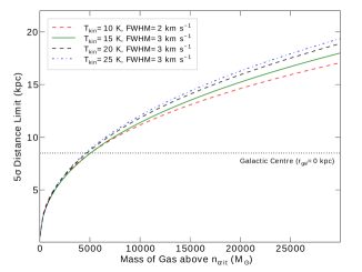
Figure 14: Plot of the 5$\sigma$ detection limit distance versus mass of gas above the NH₃ critical density ($n_{\rm crit}\approx 10^{4}\,\mbox{cm${}^{-3}$}$) for clouds with representative excitation conditions. The dotted line shows the distance of the Galactic centre at 8.5 kpc.

5.3.4 Comparison with other surveys

The only comparable single-dish NH₃ (1,1) survey conducted in the southern hemisphere is that of Hill et al. (2010) who used the Parkes radio-telescope to survey 224 high-mass starforming regions. The $\sim 1$ arcmin beam FWHM used means their data are four times less beam-diluted than HOPS and with a median $\sigma_{T_{\rm mb}}=0.05$ K the data are 4.5 times more sensitive. As a sanity check we cross-matched the HOPS NH₃ (1,1) catalogue with the 104 Hill et al. (2010) detections within the HOPS area. In total seventeen sources are matched within a $2$ arcmin radius, accounting for the brightest sources in the Hill et al. catalogue. The unmatched source tend to be weaker and we would not expect to detect them in HOPS, within the uncertainty imposed by the unknown beam-dilution factor.

5.3.5 Galactic coverage

The globally-averaged volume density of molecular clouds is typically a few $10^{2}\,\mbox{cm${}^{-3}$}$, and the distribution of molecular gas across the Galaxy is well-traced by CO emission from various surveys (e.g., Dame et al. 2001, Jackson et al. 2006). The fraction of gas in these clouds at densities of $10^{3}-10^{4}\,\mbox{cm${}^{-3}$}$, from which NH₃ emission can be detected, is usually small – of order a few percent. However, it is in the high density gas that star formation occurs. Recent studies suggest that a critical factor controlling the star formation rate within a molecular cloud is the fraction of gas above this density threshold (Lada et al., 2012). A census of this dense gas fraction is clearly very important. As a large, blind survey tracing gas at high critical density, HOPS is potentially a powerful tool for this purpose.

We have used RADEX to estimate how the 5$\sigma$ NH₃ (1,1) detection limit translates to a completeness limit for the mass of gas above the critical density ($\sim 10^{4}\,\mbox{cm${}^{-3}$}$) within molecular clouds across the Galaxy. Figure 14 illustrates the 5$\sigma$ distance limit as a function of dense gas mass for clouds with representative temperatures and linewidths. In the analysis we assume a fixed NH₃/H₂ abundance of $10^{-8}$. We expect to detect all clouds with $>$5,000 M_⊙ of dense gas which lie between the Sun and the Galactic centre. Clouds with $>$30,000 M_⊙ of dense gas will be detected at distances corresponding to the other side of the Galaxy ($d\approx 17\,$kpc). However, the distribution of molecular gas in the Galaxy is not uniform – one-third is concentrated within 3 kpc of the Galactic centre (see the model by Pohl et al. 2008). In practice this means that over 90 percent of clouds which contain $20,000\,\mbox{M${}_{\odot}$}$ of dense gas will be detected in the HOPS survey area. The HOPS survey samples approximately 66 percent of the volume of the Galaxy where molecular clouds are formed.

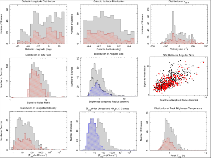
Figure 15: Properties of the clouds in the NH₃ (1,1) and (2,2) catalogues. The NH₃ (1,1) catalogue is represented by grey histograms and black symbols, while the NH₃ (2,2) catalogue is represented by red symbols and hatched histograms. In the lower-middle plot the blue hatched histogram is the subset of unresolved NH₃ (1,1) clouds. See Section 6 for details.

6 Ensemble cloud properties

In the following sections we investigate the bulk properties of the clouds in the catalogue.

6.1 Measured properties

Figure 15 presents selected plots of the measured properties for all NH₃ (1,1) and (2,2) clouds.

6.1.1 Galactic longitude and latitude

The distribution of detections as a function of Galactic longitude is shown in the top-left panel of Figure 15. Between $0^{\circ}<l<30^{\circ}$ the number of detections is relatively flat. The CMZ region, which dominated the distribution of integrated intensity in Figure 3, is detected as a single cloud, while small peaks in the distribution (e.g., at $l\approx 13.5^{\circ}$ and $l\approx 27.5^{\circ}$) are due to large star-forming complexes visible in Figure 1. The longitude range spanning $-30^{\circ}<l<-20^{\circ}$ contains the bright G333.0$-$0.4 high-mass star-forming cloud and the ‘Nessie’ filament, giving rise to the peak at $l\approx-25$. There is also a small peak in the number of detections at $l=-53\mbox{${}^{\circ}$}$, corresponding to the G305 star-forming complex and a tangent point in the Scutum-Centarus spiral arm. The longitude distributions of the NH₃ (1,1) and (2,2) catalogues show similar trends, with the NH₃ (2,2) catalogue having half as many sources per bin, as expected from the ratio of total number of sources in each catalogue. There are no detections in the $-60^{\circ}<l<-70^{\circ}$ range.

The Galactic latitude source distribution is shown in the top-centre panel of Figure 15 and is significantly biased towards negative latitudes. At $b>0.2^{\circ}$ the NH₃ (1,1) source count falls from less than 30 to approximately 20 sources per 4 arcmin bin. In contrast, no drop is seen at negative latitudes ($b<-0.2^{\circ}$), instead the source counts remain close to 45 per bin. As before both the NH₃ (1,1) and (2,2) distributions exhibit similar shapes.

6.1.2 $v_{\rm LSR}$

The distribution of brightness-weighted $v_{\rm LSR}$ over the $\pm\,200\,\mbox{km\,s${}^{-1}$}$ bandpass is shown in the top-right panel of Figure 15. Similar trends are seen between the NH₃ (1,1) and (2,2) catalogues. The histogram is dominated by the sharp peak at $\mbox{$v_{\rm LSR}$}\approx-45\,\mbox{km\,s${}^{-1}$}$. Upon examination of the full $l$-$v$ plot for the survey we see that that this feature is attributable to the sum of velocity components from the southern Galactic plane between $-70\mbox{${}^{\circ}$}<l<-20\mbox{${}^{\circ}$}$. Discounting the peak, the shape of the distribution is symmetric, with the majority of sources falling between $-100\,\mbox{km\,s${}^{-1}$}<\mbox{$v_{\rm LSR}$}<100\,\mbox{km\,s${}^{-1}$}$. The NH₃ (1,1) source count beyond $|\mbox{$v_{\rm LSR}$}|>100\,\mbox{km\,s${}^{-1}$}$ drops off rapidly from $\sim 30$ to $<5$.

6.1.3 Sensitivity and angular size

The mid-left panel of Figure 15 shows the distributions of signal-to-noise ratio (S/N = $T_{\rm mb}/\sigma_{T_{\rm mb}}$) for the NH₃ (1,1) and (2,2) clouds. In practice the brightness and size limits we imposed on the source finder mean that we are sensitive to clouds with S/N$\geq 3$, although the majority of clouds fall below S/N$\approx 20$. A typical isolated cloud detected in the NH₃ (1,1) dataset has a FWHM linewidth across the main group of $2\,\mbox{km\,s${}^{-1}$}$, equivalent to five spectral channels. Integrating the data across five channels would increase the signal-to-noise by $\sqrt{5}$ i.e. a $3\sigma$ detection would become a $6.7\sigma$ ‘integrated’ detection.

The middle panel shows the distribution of brightness-weighted radii $r_{w}$ measured from the clouds. On average the NH₃ (2,2) clouds are smaller than the (1,1) clouds. Interestingly, the NH₃ (2,2) histogram exhibits a single peak, while the NH₃ (1,1) distribution is split into two peaks of approximately resolved and unresolved sources. We attribute the excess of unresolved detections to a population of spurious sources similar to the 58 low-level detections flagged out of the NH₃ (2,2) catalogue. The thick black histogram illustrates the initial NH₃ (2,2) detections including spurious sources, flagged for having no associated NH₃ (1,1) emission. The flagged sources are clearly responsible for a second peak corresponding to an excess of unresolved sources.

The mid-right panel of Figure 15 illustrates the correlation between radius and signal-to-noise ratio. Forty-four percent of the detections in the survey are are unresolved ($r_{\rm w}<1$ arcmin) and the majority of these sources have S/N$\leq 6$.

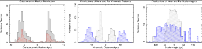
Figure 16: Left panel: Distributions of galactocentric radii for the NH₃ (1,1) (solid histogram) and (2,2) (hatched histogram) clouds. The two peaks correspond to the 5 kpc Galactic ring at positive and negative $l$. Middle panel: Distributions of near (left-slanted hatch) and far (right-slanted hatch) kinematic distances for the NH₃ (1,1) clouds calculated from the brightness-weighted $v_{\rm LSR}$. Right panel: Near and far projected Galactic scale-heights for the NH₃ (1,1) clouds. Note: In the first two panels negative values on the x-axis signify clouds in the southern Galactic plane (i.e., $l<0$). Distances were not determined for the sources with $|l|<5\mbox{${}^{\circ}$}$.

6.1.4 Integrated and peak intensity

The lower-left panel of Figure 15 shows the distribution of integrated intensities for the two catalogues. The shapes of the J,K =(1,1) and (2,2) distributions are similar, although the NH₃ (2,2) integrated intensities are weaker on average. Again the NH₃ (1,1) distribution exhibits a twin-peaked profile, which can be accounted for by the division into resolved and unresolved populations. This is demonstrated in the lower-middle panel, which plots the $\int T_{\rm mb}dv$ distribution for unresolved NH₃ (1,1) clouds overlaid on the total distribution. The unresolved subset clearly corresponds to the less intense peak, which likely contains significant numbers of spurious sources.

The difference in the integrated intensities is in part due to the higher average brightness temperature of the NH₃ (1,1) line, as shown in the bottom-right panel of Figure 15. The NH₃ (1,1) and (2,2) distributions exhibit similar shapes, although the median $T_{\rm mb}$ for the J,K =(1,1) transition is 0.99 K compared to 0.87 K for (2,2).

6.2 Kinematic distance and Galactic structure

The Galactic disk has a well measured rotation curve which can be used to solve for an approximate ‘kinematic’ distance given a line-of-site velocity towards a particular Galactic longitude. This method has the disadvantage that sources located within the radius of the Sun’s orbit have two valid distance solutions, requiring further information to distinguish between the near and far distances. In addition, local velocity deviations due to streaming motions in Galactic spiral arms lead to a distance uncertainty of order $\pm 1$ kpc (e.g., Nguyen Luong et al. 2011).

Outside the CMZ the NH₃ (1,1) spectra of most clouds exhibit uncomplicated line profiles (i.e., moderate optical depth with only one or two velocity components) and the measured $v_{\rm LSR}$ is an accurate representation of the cloud systemic velocity. Distance estimates made using NH₃ lines are hence more accurate than those made using optically-thick tracers (e.g., CO (1 – 0)), whose line profiles may be severely distorted. Bright maser lines (e.g., the 22 GHz H₂O line) have the advantage of being detectable at further distances, however, individual spectral components are often offset from the systemic velocity by greater than 15 km s^-1 (e.g., Caswell & Phillips 2008).

6.2.1 Kinematic distance

Using the rotation curve of Brand & Blitz (1993) and the intensity weighted $l$-$b$-$v$ coordinates we have derived the unique galactocentric radius, near and far kinematic distances, and projected scaleheights for each NH₃ cloud. The model assumes a distance to the Galactic centre of 8.5 kpc and a solar velocity of $220\,\mbox{km\,s${}^{-1}$}$. Although recent work, such as by Reid et al. (2009), has suggested that the Solar rotational velocity is higher than the IAU value of 220 km s^-1, for simplicity we adopt the rotational velocity of the original model. A more detailed analysis incorporating the recent developments will be presented in a future paper. Galactic rotation is known to depart from the approximations of rotation curves towards the inner Galaxy, as such we omit sources between $-5\mbox{${}^{\circ}$}<l<5\mbox{${}^{\circ}$}$. Kinematic distance estimates were determined for 576 clouds (86 %) and are recorded in the online version of the HOPS catalogue. The left panel of Figure 16 shows the distribution of galactocentric radii for the NH₃ (1,1) and (2,2) clouds, with negative values indicating positions in the southern Galactic plane ($l<0$). The NH₃ (1,1) and (2,2) distributions are similar and we continue our analysis using the NH₃ (1,1) clouds only, as they are more numerous. The two strong peaks at approximately $-5.7$ kpc and $+4.2$ kpc correspond to the so called ‘Galactic ring’ feature, a region that is most likely a supposition of several spiral arms, and which is thought to contain most of the molecular gas outside of Central Molecular Zone (Burton et al., 1975; Scoville & Solomon, 1975). The difference in the galactocentric radii of the peaks may be attributed to the negatively-biased longitude coverage, but it is also consistent with their origin in an asymmetric structure, such as a spiral arm.

In the middle panel are plotted histograms of near and far kinematic distances for the NH₃ (1,1) detections. By design the two distributions have very little overlap, with most near distances falling between two and eight kpc (inside the tangent circle), and most far distances between eight and fourteen kpc. Clouds with masses or kinetic temperatures bright enough to be detected beyond the Galactic centre will be necessarily rare (see Figure 14), implying that the near distance is favoured for the majority of sources. Support for choosing the near kinematic distances in at least half of the NH₃ (1,1) detections comes from comparing the catalogue with infrared dark clouds (IRDCs). IRDCs are seen as dark extinction features against the bulk of diffuse Galactic infrared emission and, due to their nature, are thought to lie at near kinematic distances (Simon et al., 2006). We cross-matched the NH₃ (1,1) catalogue with the list of IRDCs compiled by Simon et al. (2006) from the 8.3 $\micron$ Midcourse Space Experiment (MSX) images. Fifty percent of the NH₃ (1,1) cloud centres were found to lie within 2 arcmin of an IRDC extinction peak, confirming their association.

We urge caution in considering the scale-height distribution of clouds in HOPS. The $b\pm 0.5\mbox{${}^{\circ}$}$ coverage likely truncates the true distribution of molecular gas, as evidenced by the flat emission profile in Figure 3. Near and far scale-heights are plotted in the right-panel of Figure 16 and have standard-deviations of 13.1 pc and 30.9 pc, respectively. Both values are within the expected scaleheights of massive star-formation tracers found in the literature, e.g., Urquhart et al. (2011) measured an average scaleheight of $29\pm 0.5$ pc for massive young stellar objects in the Red MSX source survey.

6.2.2 Galactic structure

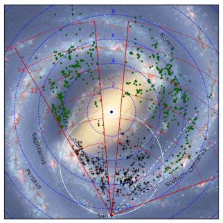
Figure 17: Face-on artistic rendering of the Galaxy showing the positions of the clouds found by HOPS at the near and far kinematic distances (black crosses and green circles, respectively). This plot is modeled after Figure 9 of Urquhart et al. (2011). Dotted lines mark the distance from the Galactic centre (blue) and the Sun (red) in kiloparsecs. The four main spiral-arms are labeled in black text. The position of the rotational tangent point is delineated by a white circle.

Figure 17 illustrates the positions of the NH₃ (1,1) clouds on an artists rendering of the Galaxy as viewed face-on. The image has been constructed by Robert Hurt of the Spitzer Science Centre in collaboration with Robert Benjamin of the University of Wisconsin-Whitewater and attempts to include the most recent information on Galctic structure. The key features are two ‘major’ spiral-arms (Scutum-Centarus and Perseus), two minor spiral arms (Norma and Sagittarius) and nested Galactic bars: a long (thin) bar at an angle of $\sim 45\mbox{${}^{\circ}$}$ to the sun-centre line (Hammersley et al., 2000; Benjamin et al., 2005; Cabrera-Lavers et al., 2008) and a short (boxy/bulge) bar at an orientation of $20\,-\,30\mbox{${}^{\circ}$}$ (Blitz & Spergel, 1991; Weiland et al., 1994). Both near and far kinematic distances have been plotted as black crosses and green circles, respectively. For clouds within $-30\mbox{${}^{\circ}$}<l<30\mbox{${}^{\circ}$}$ the near and far distances are widely separated, with the majority of the far distances lying well beyond our 3.2 kpc sensitivity limit for 400 M_⊙ objects. If we assume near distances are correct, then the cluster of sources between $23\mbox{${}^{\circ}$}<l<30\mbox{${}^{\circ}$}$ and at a distance of 6 kpc line up with the intersection of the long-bar and the Scutum-Centarus spiral arm. Urquhart et al. (2011) also found a large number of high-mass stars concentrated in this region, while the BUFCRAO Galactic Ring Survey (Roman-Duval et al., 2009) reported a large amount of molecular material in approximately the same area.

Clouds between $-55\mbox{${}^{\circ}$}<l<-40\mbox{${}^{\circ}$}$ (between white dashed lines in Figure 17) correlate well with the Scutum-Centarus spiral arm when placed at the far distance, and would otherwise fall between arms.

A more thorough investigation of the near/far distance ambiguity will be the subject of a future paper at which time we will be in a position to comment on Galactic structure with greater authority.

7 Summary and future work

We have mapped 100 square degrees of the Galactic plane in the J,K = (1,1) and (2,2) transitions of NH₃ at a resolution of $2$ arcmin using the Mopra radio-telescope. The survey covers the region $-70\mbox{${}^{\circ}$}<l<30\mbox{${}^{\circ}$}$, $|b|<0.5\mbox{${}^{\circ}$}$ with a velocity range of $\pm 200\,\mbox{km\,s${}^{-1}$}$. The median sensitivity is $\sigma_{T_{\rm mb}}=0.20\pm 0.06$ K in each $0.42\,\mbox{km\,s${}^{-1}$}$ spectral channel. We have developed an automatic emission-finding routine based on DUCHAMP and used it to find clouds of contiguous emission in the $l$-$b$-$v$ data cubes. The following are our main findings:

1. We have detected NH₃ emission across the Galactic longitude range between $-60\mbox{${}^{\circ}$}<l<30\mbox{${}^{\circ}$}$, however, the outer Galaxy between $-70\mbox{${}^{\circ}$}<l<-60\mbox{${}^{\circ}$}$ is devoid of emission above our sensitivity limit. The Central Molecular Zone (CMZ, $|l|<2\mbox{${}^{\circ}$}$) contains 80.6 percent of the NH₃ (1,1) integrated intensity, which appears as a single giant cloud at 2 arcmin resolution. Most of the remaining gas is concentrated within $2\mbox{${}^{\circ}$}<|l|<30\mbox{${}^{\circ}$}$. Within the CMZ the NH₃ (1,1) integrated intensity peaks near the Galactic midplane, but the distribution with $b$ is largely flat outside the CMZ.

2. Using our emission-finding procedure we detected 669 NH₃ (1,1) clouds and 248 NH₃ (2,2) clouds, and measured their basic properties. Forty-four percent of the NH₃ (1,1) clouds are unresolved in the 2 arcmin Mopra beam. The full HOPS NH₃ (1,1) catalogue likely contains significant numbers of unresolved spurious sources below $5\sigma$. However, a high-reliability catalogue may be constructed by restricting the number of pixels required in a detection to 13, reducing the source-count by 20 percent.

3. The NH₃ catalogue contains clouds detected down to a 3$\sigma$ level (0.6 K) where it is 60 percent complete. The catalogue is $\sim 100$ percent complete at the 5$\sigma$ level (1.0 K). As an illustration of the sensitivity, we would detect a typical 400 M_⊙ NH₃ (1,1) cloud (T${}_{\rm kin}=20$ K, $n_{\rm H_{2}}=10^{4}\mbox{cm${}^{-3}$}$) out to a distance of 3.2 kpc at the 5$\sigma$ level. Similar clouds containing 5,000 M_⊙ and 30,000 M_⊙ would be detected at the Galactic centre and on the far side of the Galaxy, respectively.

4. We have estimated the near and far kinematic distances towards the NH₃ (1,1) clouds. Given our sensitivity limits the majority of clouds likely lie at the near distance. Sources between $-55\mbox{${}^{\circ}$}<l<-40\mbox{${}^{\circ}$}$ may lie at either the near or far distance in the Scutum-Centarus spiral arm. Further investigation is required to distingush between the two possibilities.

Combined with other Galactic plane surveys the HOPS catalogues provide an invaluable tool for the investigation of Galactic structure and evolution. The next paper in the series (Longmore et al. in prep.) will present an analysis of the NH₃ spectra, the physical and evolutionary status of the detected clouds, and the procedures developed to automate the line fitting. Further papers will publish the other spectral lines observed, including the J,K = (3,3) (6,6) and (9,9) NH₃ transitions, HC₃N (3,2) and H69$\alpha$.

7.1 Data release

The NH₃ data and cloud catalogues are available to the community from the HOPS website, http://www.hops.org.au, via an automated cutout server and catalogue files. In addition to the FITS format data-cubes we have made available the emission-finder masks, integrated intensity and peak temperature maps. Interested parties may also download the emission-finding and baseline-fitting procedures, which have been written in the python language.

Table 2: Properties of the NH₃ (1,1) clouds identified in HOPS.

	Weighted			Peak
Cloud Name∗	$l$	$b$	$v_{\rm LSR}$	$l$	$b$	$v_{\rm LSR}$	$v_{\rm min}$	$v_{\rm max}$	$r_{\rm c}$	$r_{\rm w}$	$\Omega$	npix	nvox	$\int T_{\rm mb}dv$	$T_{\rm peak}$	$T_{\rm RMS}$	Flags†
	(∘)	(∘)	(km s-1)	(∘)	(∘)	(km s-1)	(km s-1)		(′)	(′)	$arcmin^{2}$			(K km s-1)	(K)	(K)
(1)	(2)	(3)	(4)	(5)	(6)	(7)	(8)	(9)	(10)	(11)	(12)	(13)	(14)	(15)	(16)	(17)	(18)
${\rm G029.987-0.157+097.3}$	29.986	-0.156	97.3	29.992	-0.143	98.0	96.3	98.0	1.2	0.8	4.75	19	76	7.38 $\pm$ 0.61	0.74	0.16
${\rm G018.122+0.359+022.4}$	18.122	0.359	22.5	18.125	0.357	23.0	11.5	23.4	1.6	1.0	8.25	33	83	9.75 $\pm$ 0.53	0.66	0.14
${\rm G008.621-0.346+037.3}$	8.622	-0.349	37.5	8.700	-0.401	39.2	12.3	60.5	9.4	8.1	275.50	1102	18506	2751.12 $\pm$ 10.16	2.17	0.17	X
${\rm G002.507-0.032-02.0}$	2.505	-0.029	-2.4	2.508	-0.026	-9.0	-27.7	20.9	4.0	1.9	49.25	197	8250	962.50 $\pm$ 7.43	1.31	0.19				E
${\rm G000.860-0.067+045.7}$	0.807	-0.064	47.5	359.875	-0.084	11.9	-138.5	146.6	34.5	28.7	3748.00	14992	2114971	443317.78 $\pm$ 113.19	6.40	0.18	X		M	E
${\rm G359.084+0.108+139.3}$	359.078	0.109	138.9	359.042	0.141	130.8	108.7	165.4	5.4	3.1	91.00	364	17181	2612.32 $\pm$ 12.95	1.56	0.23			M	E
${\rm G343.423-0.352-27.3}$	343.423	-0.351	-27.2	343.425	-0.343	-27.3	-46.5	-7.3	3.7	2.0	42.00	168	920	182.69 $\pm$ 2.99	1.54	0.23
${\rm G302.008+0.058+198.1}$	302.008	0.058	198.1	302.008	0.049	197.8	197.8	198.2	0.9	0.5	2.50	10	13	1.10 $\pm$ 0.32	0.60	0.21		Z

^∗ The cloud is named for the centroid position in $l$-$b$-$v$ space.
^† The flags in column (18) have the following meanings: X = the cloud touches a Galactic longitude boundary, Y = the cloud touches a Galactic latitude boundary, Z = the cloud touches a velocity boundary ($\pm$ 200 km s^-1). M = multiple velocity components along the line of sight, E = an extended cloud which may contain multiple sub-clouds, A = a cloud identified as artefacts (e.g., invading NH₃ (2,2) emission or up-turned bandpass-edges).

Table 3: Properties of the NH₃ (2,2) clouds identified in HOPS.

	Weighted			Peak
Cloud Name∗	$l$	$b$	$v_{\rm LSR}$	$l$	$b$	$v_{\rm LSR}$	$v_{\rm min}$	$v_{\rm max}$	$r_{\rm c}$	$r_{\rm w}$	$\Omega$	npix	nvox	$\int T_{\rm mb}dv$	$T_{\rm peak}$	$T_{\rm RMS}$	Flags†
	(∘)	(∘)	(km s-1)	(∘)	(∘)	(km s-1)	(km s-1)		(′)	(′)	$arcmin^{2}$			(K km s-1)	(K)	(K)
(1)	(2)	(3)	(4)	(5)	(6)	(7)	(8)	(9)	(10)	(11)	(12)	(13)	(14)	(15)	(16)	(17)	(18)
${\rm G029.995+0.156-84.1}$	29.994	0.156	-84.1	29.992	0.166	-39.2	-84.4	-83.6	0.7	0.5	1.75	7	12	0.86 $\pm$ 0.27	0.71	0.18				E
${\rm G023.332-0.253+096.4}$	23.333	-0.253	96.4	23.267	-0.243	60.5	78.0	102.3	2.0	1.5	12.25	49	120	16.45 $\pm$ 0.85	0.90	0.18				E
${\rm G018.859-0.477+065.3}$	18.860	-0.476	65.4	18.883	-0.476	65.6	55.8	68.2	2.8	2.0	24.00	96	677	136.29 $\pm$ 2.86	1.85	0.26	X
${\rm G009.125-0.153+043.7}$	9.125	-0.154	43.7	9.117	-0.159	43.9	43.5	43.9	0.7	0.4	1.75	7	11	1.45 $\pm$ 0.27	0.80	0.19
${\rm G000.892-0.057+050.7}$	0.819	-0.060	49.7	359.875	-0.084	13.2	-128.7	152.6	32.6	27.5	3339.00	13356	1640704	274605.81 $\pm$ 91.23	4.96	0.17	X		M	E
${\rm G338.920-0.483-36.8}$	338.922	-0.482	-36.9	338.942	-0.484	-37.5	-37.9	-35.8	1.9	1.2	11.50	46	175	16.41 $\pm$ 1.04	1.17	0.18	X
${\rm G322.258+0.166-171.2}$	322.258	0.166	-171.2	322.258	0.166	-171.8	-171.8	-170.9	0.9	0.5	2.50	10	20	2.02 $\pm$ 0.31	0.67	0.16		Z
${\rm G300.464-0.498-198.0}$	300.464	-0.497	-198.0	300.450	-0.493	-198.2	-198.2	-197.8	0.9	0.8	2.75	11	21	2.40 $\pm$ 0.40	1.41	0.21	X	Z

^∗, ^† Annotation markings have the same meanings as in Table 2.

Appendix A Spectral baselines

Figure 18: Integrated spectrum measured from an area of emission close to the Galactic centre. The spectrum in the top panel is drawn from the data baselined using only a 1^st order polynomial in livedata. The spectrum in the bottom panel has had further baselines subtracted using the ASAP fitting software.

During the initial data reduction, the LIVEDATA software was used to fit and subtract a first order polynomial from the line free channels of the spectra. In the majority of cases this was more than sufficient to flatten the baselines, however, we occasionally found that two types of baseline artifacts remain:

1. Ripples and sine-waves caused by rapidly changing weather conditions.

2. Negative bowls adjacent to very broad spectral lines in the vicinity of the Galactic centre.

Type (i) artifacts are likely to contaminate the catalogue with spurious sources where the peaks of the ripples rise above the noise. To mitigate against this problem we utilised the ATNF ASAP package to fit additional polynomials of order 3 – 5 to the data. Before performing the fit, any bright spectral lines were masked off using a prior duchamp-produced mask. This approach was entirely successful in eliminating these baseline artifacts.

Broad-line sources with type (ii) artifacts tend to have artificially clipped boundaries and suppressed flux densities. Figure 18 shows examples of integrated spectra measured close to the Galactic centre. The spectrum in the top panel is extracted from data processed using livedata and gridzilla only. livedata cannot identify broad spectral features and so fits the wings of these lines as part of the emission-free baseline, suppressing the real baseline below zero. In order to zero the baselines we iterated around the following procedure until no further improvement was seen:

• Run the emission finder to produce an emission mask.

• Expand the cloud masks by ten percent in $l$-$b$-$v$ .

• Mask the emission and fit a first-order polynomial to the line-free channels.

The solid line in the bottom panel of Figure 18 shows the same spectrum after three iterations of fitting. All negative bowls were successfully eliminated from the cubes.

Appendix B Running the Duchamp emission finder

Table 4: Critical inputs to the DUCHAMP emission finder (version 1.1.10).

Input Name	Value	Notes
flagAtrous	Yes	Perform the à trous wavelet reconstruction.
reconDim	3	Reconstruct the data in 3D mode.
scaleMin, Max	1 – 0	Automatically determine which wavelet scales to be included in the reconstructed image.
snrRecon	10	Signal-to-noise ratio required to include a wavelet coefficient at a point in the reconstructed cube.
filterCode	1	Use a B3 spline filter in the reconstruction.
searchType	Spatial	Search one channel-map at a time.
threshold	0.8	Search the signal-to-noise cube to a level of 0.8-$\sigma$.
flagGrowth	False	Do not ‘grow’ clumps to a lower threshold.
threshSpatial	2	Merge clumps within two spatial pixels.
threshVelocity	53 (68)	Merge clumps within 53 channels (22.3 km s-1), the velocity difference between the central and outer
		satellite groups in the NH3 (1,1) spectrum, plus a 3 km s-1 guard band. For NH3 (2,2) the threshold
		is 68 channels (29.0 km s-1).
minChannels	2	Require a valid detection to span at least two channels (0.85 km s-1).
minPix	7	Require a detection to contain at least seven spatial pixels.

For detailed information on the duchamp algorithm and settings the reader is referred to the duchamp web page and user-guide linked therein. Here we detail how the emission finder was used with the HOPS NH₃ data.

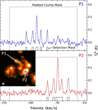
Figure 19: The inset image shows an integrated intensity map of NH₃ emission in the G333 cloud. The green contour represents the cloud boundary. duchamp detects each of the NH₃ (1,1) spectral line components individually (top and bottom panels), however, the sub-clouds overlap both spatially and in velocity and are hence catalogued as a single merged cloud.

At the outset the reconstructed signal-to-noise cube is searched one spectral plane at a time down to a global brightness threshold. Voxels containing emission above the threshold are recorded and grouped with their immediate neighbours. The list of detections is condensed by rigorously merging adjacent objects within two spatial pixels (1’ = 1/2 beam FWHM) or within the velocity spread of the NH₃ spectrum. The expected velocity limits correspond to the frequency difference between the main and outer satellite groups, plus a guard band to account for the width of the lines. For NH₃ (1,1) this $\sim 19.7\,\mbox{km\,s${}^{-1}$}$ plus $3.0\,\mbox{km\,s${}^{-1}$}$ (= 53 channels) and for NH₃ (2,2) $\sim 26.0\,\mbox{km\,s${}^{-1}$}$ plus $3.0\,\mbox{km\,s${}^{-1}$}$ (= 68 channels). duchamp makes no attempt to separate contiguous areas of emission into components in the manner of clumpfind (Williams et al., 1994) or fellwalker. Adjacent regions of emission in which the outer satellite lines overlap are merged into a single object in the resultant catalogue. Figure 19 shows an example of an emitting region containing several distinct velocity components which are counted as a single cloud by duchamp.

When the merging is completed further criteria are applied which filter out emission significantly smaller than the beam ($<$7 pixels), or with unusually narrow linewidths ($<$ 2 channels, i.e., a minimum width of $0.84\,\mbox{km\,s${}^{-1}$}$). Finally a mask cube is created which uses unique integers to identify the contiguous emitting regions.

To facilitate the measurement and analysis steps the final mask cube is used as a template to excise each duchamp cloud from the original HOPS NH₃ data-cubes. Small FITS cubes are produced containing one cloud each in addition to 2- and 3-D masks indicating which pixels/voxels contain emission.

B.1 Emission finder inputs

The critical inputs for the second pass of DUCHAMP are presented in Table 4. These are correct for DUCHAMP version 1.1.10. Before running the finder we performed the à trous reconstruction on the data as it confers a considerable advantage in detecting compact and weak emission. The ideal reconstruction parameters are dependant on the noise properties of the cubes and we experimented with different values of snrRecon, scaleMax and filterCode (see Table 4) until the residuals contained only noise. The search threshold was based on completeness tests performed using artificial sources injected into the data (see Section 5.3.1). A 0.8$\sigma$ threshold was used, equivalent to $\sim$ 0.16 K and sensitive enough to sample the completeness curve below the one percent level. The last critical parameter is minimum number of pixels required in a detection. With a beam-size of $\Theta_{\rm\,FWHM}$ = 2 arcmin and pixel dimensions of $\Delta_{pix}=0.5$ arcmin, there are 12.6 pixels within the solid angle subtended by the beam FWHM. For weak and unresolved emission we may only detect the peak of the beam function, hence we set a threshold of seven pixels per beam. We justify our input criteria fully in Section 5.3.1.

References

- Bains et al. (2006) Bains I., Wong T., Cunningham M., Sparks P. Ellingsen S., Fulton B., Herpin F., Jones P., thirteen others. 2006, MNRAS, 367, 1609
- Bally et al. (2010) Bally J., Aguirre J., Battersby C., Bradley E. T., Cyganowski C., Dowell D., Drosback M., Dunham M. K., Evans II N. J., Ginsburg A., Glenn J., Harvey P., Mills E., Merello M., Rosolowsky E., Schlingman W., 2010, ApJ, 721, 137
- Bania (1977) Bania T. M., 1977, ApJ, 216, 381
- Benjamin et al. (2005) Benjamin R. A., Churchwell E., Babler B. L., Indebetouw R., Meade M. R., Whitney B. A., Watson C., Wolfire M. G., Wolff M. J., Ignace R., Bania T. M., Bracker S., Clemens D. P., Chomiuk L., Cohen M., Dickey J. M., Jackson J. M., five others. 2005, ApJ, 630, L149
- Bergin et al. (2006) Bergin E. A., Maret S., van der Tak F. F. S., Alves J., Carmody S. M., Lada C. J., 2006, ApJ, 645, 369
- Blitz & Spergel (1991) Blitz L., Spergel D. N., 1991, ApJ, 379, 631
- Brand & Blitz (1993) Brand J., Blitz L., 1993, A&A, 275, 67
- Burton et al. (1975) Burton W. B., Gordon M. A., Bania T. M., Lockman F. J., 1975, ApJ, 202, 30
- Cabrera-Lavers et al. (2008) Cabrera-Lavers A., González-Fernández C., Garzón F., Hammersley P. L., López-Corredoira M., 2008, A&A, 491, 781
- Caswell & Phillips (2008) Caswell J. L., Phillips C. J., 2008, MNRAS, 386, 1521
- Clark & Porter (2004) Clark J. S., Porter J. M., 2004, A&A, 427, 839
- Dame et al. (1986) Dame T. M., Elmegreen B. G., Cohen R. S., Thaddeus P., 1986, ApJ, 305, 892
- Dame et al. (2001) Dame T. M., Hartmann D., Thaddeus P., 2001, ApJ, 547, 792
- Hammersley et al. (2000) Hammersley P. L., Garzón F., Mahoney T. J., López-Corredoira M., Torres M. A. P., 2000, MNRAS, 317, L45
- Hill et al. (2010) Hill T., Longmore S. N., Pinte C., Cunningham M. R., Burton M. G., Minier V., 2010, MNRAS, 402, 2682
- Hindson et al. (2010) Hindson L., Thompson M. A., Urquhart J. S., Clark J. S., Davies B., 2010, MNRAS, 408, 1438
- Ho & Townes (1983) Ho P. T. P., Townes C. H., 1983, ARA&A, 21, 239
- Jackson et al. (2010) Jackson J. M., Finn S. C., Chambers E. T., Rathborne J. M., Simon R., 2010, ApJ, 719, L185
- Jackson et al. (2006) Jackson J. M., Rathborne J. M., Shah R. Y., Simon R., Bania T. M., Clemens D. P., Chambers E. T., Johnson A. M., Dormody M., Lavoie R., Heyer M. H., 2006, ApJS, 163, 145
- Kutner & Ulich (1981) Kutner M. L., Ulich B. L., 1981, ApJ, 250, 341
- Lada et al. (2012) Lada C. J., Forbrich J., Lombardi M., Alves J. F., 2012, ApJ, 745, 190
- Ladd et al. (2005) Ladd E. F., Purcell C. R., Wong T., Robertson S., 2005, PASA, 22, 62
- Lo et al. (2009) Lo N., Cunningham M. R., Jones P. A., Bains I., Burton M. G., Wong T., Muller E., Kramer C., Ossenkopf V., Henkel C., Deragopian G., Donnelly S., Ladd E. F., 2009, MNRAS, 395, 1021
- Longmore et al. (2007) Longmore S. N., Burton M. G., Barnes P. J., Wong T., Purcell C. R., Ott J., 2007, MNRAS, 379, 535
- Morgan et al. (2010) Morgan L. K., Figura C. C., Urquhart J. S., Thompson M. A., 2010, MNRAS, 408, 157
- Morris & Serabyn (1996) Morris M., Serabyn E., 1996, ARA&A, 34, 645
- Nguyen Luong et al. (2011) Nguyen Luong Q., Motte F., Schuller F., Schneider N., Bontemps S., Schilke P., Menten K. M., Heitsch F., Wyrowski F., Carlhoff P., Bronfman L., Henning T., 2011, A&A, 529, A41
- Pickett et al. (1998) Pickett H. M., Poynter R. L., Cohen E. A., Delitsky M. L., Pearson J. C., Muller H. S. P., 1998, J. Quant. Spectrosc. & Rad. Transfer, 60, 883
- Pohl et al. (2008) Pohl M., Englmaier P., Bissantz N., 2008, ApJ, 677, 283
- Purcell et al. (2009) Purcell C. R., Minier V., Longmore S. N., André P., Walsh A. J., Jones P., Herpin F., Hill T., Cunningham M. R., Burton M. G., 2009, A&A, 504, 139
- Reid et al. (2009) Reid M. J., Menten K. M., Zheng X. W., Brunthaler A., Moscadelli L., Xu Y., Zhang B., Sato M., Honma M., Hirota T., Hachisuka K., Choi Y. K., Moellenbrock G. A., Bartkiewicz A., 2009, ApJ, 700, 137
- Rodriguez-Fernandez & Combes (2008) Rodriguez-Fernandez N. J., Combes F., 2008, A&A, 489, 115
- Roman-Duval et al. (2009) Roman-Duval J., Jackson J. M., Heyer M., Johnson A., Rathborne J., Shah R., Simon R., 2009, ApJ, 699, 1153
- Rydbeck et al. (1977) Rydbeck O. E. H., Sume A., Hjalmarson A., Ellder J., Ronnang B. O., Kollberg E., 1977, ApJ, 215, L35
- Scoville & Solomon (1975) Scoville N. Z., Solomon P. M., 1975, ApJ, 199, L105
- Simon et al. (2006) Simon R., Jackson J. M., Rathborne J. M., Chambers E. T., 2006, ApJ, 639, 227
- Simon et al. (2006) Simon R., Rathborne J. M., Shah R. Y., Jackson J. M., Chambers E. T., 2006, ApJ, 653, 1325
- Starck & Murtagh (1994) Starck J.-L., Murtagh F., 1994, A&A, 288, 342
- Urquhart et al. (2010) Urquhart J. S., Hoare M. G., Purcell C. R., Brooks K. J., Voronkov M. A., Indermuehle B. T., Burton M. G., Tothill N. F. H., Edwards P. G., 2010, PASA, 27, 321
- Urquhart et al. (2011) Urquhart J. S., Moore T. J. T., Hoare M. G., Lumsden S. L., Oudmaijer R. D., Rathborne J. M., Mottram J. C., Davies B., Stead J. J., 2011, MNRAS, 410, 1237
- van der Tak et al. (2007) van der Tak F. F. S., Black J. H., Schöier F. L., Jansen D. J., van Dishoeck E. F., 2007, A&A, 468, 627
- Walsh et al. (2011) Walsh A. J., Breen S. L., Britton T., Brooks K. J., Burton M. G., Cunningham M. R., Green J. A., Harvey-Smith L., Hindson L., Hoare M. G., Indermuehle B., Jones P. A., Lo N., Longmore S. N., Lowe V., Phillips C. J., Purcell C. R., five others 2011, MNRAS, 416, 1764
- Walsh et al. (2008) Walsh A. J., Lo N., Burton M. G., White G. L., Purcell C. R., Longmore S. N., Phillips C. J., Brooks K. J., 2008, Publications of the Astronomical Society of Australia, 25, 105
- Weiland et al. (1994) Weiland J. L., Arendt R. G., Berriman G. B., Dwek E., Freudenreich H. T., Hauser M. G., Kelsall T., Lisse C. M., Mitra M., Moseley S. H., Odegard N. P., Silverberg R. F., Sodroski T. J., Spiesman W. J., Stemwedel S. W., 1994, ApJ, 425, L81
- Whiting (2012) Whiting M. T., 2012, MNRAS, 421, 3242
- Williams et al. (1994) Williams J. P., de Geus E. J., Blitz L., 1994, ApJ, 428, 693
- Wong et al. (2008) Wong T., Ladd E. F., Brisbin D., Burton M. G., Bains I., Cunningham M. R., Lo N., Jones P. A., Thomas K. L., Longmore S. N., Vigan A., Mookerjea B., Kramer C., Fukui Y., Kawamura A., 2008, MNRAS, 386, 1069