Long time asymptotics of the totally asymmetric
simple exclusion process

Abstract

We study the long time asymptotics of the relaxation dynamics of the totally asymmetric simple exclusion process on a ring. Evaluating the asymptotic amplitudes of the local currents by the algebraic Bethe ansatz method, we find the relaxation times starting from the step and alternating initial conditions are governed by different eigenvalues of the Markov matrix. In both cases, the scaling exponents of the leading asymptotic amplitudes with respect to the total number of sites are found to be $-1$. We also study the asymptotics of correlation functions such as the emptiness formation probability.

PACS numbers: 02.30.Ik, 02.50.Ey, 05.70.Ln

1 Introduction

The asymmetric simple exclusion process (ASEP) is one of the most fundamental models in nonequilibrium statistical mechanics [1, 2, 3, 4, 5]. The ASEP is a stochastic interacting particle system consisting of biased random walkers obeying the exclusion principle, and have applications to biology [6], traffic flows [7, 8] and quantum dots [9], for example. Like the Ising model in equilibrium statistical mechanics, the ASEP is nowadays a paradigm in nonequilibrium statistical mechanics in the sense that many exact methods are amenable to extract various interesting nontrivial facts. For example, the matrix product representation [10, 11, 12, 13, 14, 15] of the steady state revealed boundary induced phase transitions [16]. For the last ten years, due to the development of the random matrix theory [17, 18, 19, 20, 21, 22, 23, 24], the current fluctuations in the infinite system were shown to satisfy the Tracy-Widom distribution.

The Bethe ansatz method, which was originated as a traditional method to analyze quantum integrable models such as the Heisenberg XXZ chain, can also be applied to analyze the ASEP. This comes from the fact that the Markov matrix describing the dynamics of the ASEP is equivalent to the Hamiltonian of an integrable spin chain. Utilizing this fact, the relaxation times and spectral gaps were examined [25, 26, 27, 28, 29, 30, 31, 32, 33], and the exact expression for cumulants of currents and large deviation functions were obtained [34, 35, 36, 37, 38].

One of the latest developments of the Bethe ansatz approach is the study of the full relaxation dynamics of the totally asymmetric simple exclusion process (TASEP) on a ring by the algebraic Bethe ansatz method [39]. Previously, by noting the equivalence between the Markov matrix of the TASEP and the Hamiltonain of an integrable spin chain, the algebraic Bethe ansatz derivation of the Bethe ansatz equation and the construction of the determinant representation of the scalar product [40, 41, 42] was done. However, the power of the algebraic Bethe ansatz method was not fully utilized to study the dynamics of the TASEP, due to the difficulties of evaluating the multipoint form factors and the overlap between the initial state and the Bethe vector. Formulating the dynamics of the TASEP by evaluating the form factors and the overlap from the algebraic Bethe ansatz, we examined the full relaxtion dynamics of the local densities and currents, and found the scaling exponents of the asymptotic amplitudes starting from the step initial condition for example. The Monte Carlo method can be employed to study the full relaxation dynamics as well, but it is difficult to study the details of the dynamics, the long time asymptotics for example.

In this paper, we study the long time behavior of the relaxation dynamics to the steady state by the algebraic Bethe ansatz method. We particularly focus on the local currents, and the two fundamental initial conditions: the step and the alternating initial conditions. The step initial condition is the case which the half of the system is consecutively occupied by the particles and the other half is empty at the initial time. The alternating initial condition is the case which all odd sites are occupied while all even sites are empty. We examine the asymptotic amplitudes of the local currents, and find that in contrast to the step initial condition, the asymptotic amplitudes corresponding to the lowest excited states of the Markov matrix vanish for the alternating initial condition. In other words, the relaxation time of the alternating initial condition is not governed by the lowest excited states. Instead, the second lowest excited state determines the relaxation time. Our discovery suggests that the naive guess of the relaxation time by considering only the Markov matrix may lead to an incorrect result.

This paper is organized as follows. In the next section, we review the basics of the algebraic Bethe ansatz and the scalar products. In section 3, we formulate the dynamics of the local densities, currents and the emptiness formation probability of the TASEP by the algebraic Bethe ansatz method. This is achieved by evaluating the form factors and the overlap between the initial state and arbitrary Bethe vector for the case of step and alternating initial conditions. The low excited states of the Markov matrix are described in section 4. The long time asymptotics for the step initial condition is analyzed in section 5. In section 6, we analyze the alternating initial condition and extract interesting difference from the step initial condition. Section 5 is devoted to the conclusion.

2 Algebraic Bethe ansatz of the TASEP

In this and the next sections, we formulate the dynamics of the TASEP on a periodic ring by the algebraic Bethe ansatz method. In this section, we review the relation between the TASEP and the integrable spin chain, and the basics of the algebraic Bethe ansatz and the scalar products.

2.1 The definition of the TASEP

We consider the TASEP on a periodic ring with $M$ sites and $N$ particles. Since the particles obey the exclusion rule, each site can be occupied by at most one particle. The dynamical rule of the TASEP is as follows: during the time interval $\mathrm{d}t$, a particle at a site $j$ jumps to $(j+1)$th site with probability $\mathrm{d}t$, if the $(j+1)$th site is vacant. For convenience, we associate a Boolean variable $\tau_{i}$ to every site $i$ to indicate whether a particle is present $(\tau_{i}=1)$ or not $(\tau_{i}=0)$. The probability of being in the (normalized) state $|\tau_{1},\dots,\tau_{M}\rangle$ is denoted as $P_{t}(\tau_{1},\dots,\tau_{M})$. The time evolution of the state vector $|\psi(t)\rangle=\sum_{\tau_{i}=0,1}P_{t}(\tau_{1},\dots,\tau_{M})|\tau_{1},\dots,\tau_{M}\rangle$ is subject to the master equation

$$\frac{\mathrm{d}}{\mathrm{d}t}|\psi(t)\rangle=\mathcal{M}|\psi(t)\rangle.$$ (1)

Here the Markov matrix $\mathcal{M}$ of the TASEP is defined by

$$\mathcal{M}=\sum_{j=1}^{M}\Bigg{\{}\sigma_{j}^{+}\sigma_{j+1}^{-}+\frac{1}{4}(\sigma_{j}^{z}\sigma_{j+1}^{z}-1)\Bigg{\}},$$ (2)

where $\sigma_{j}^{\pm}:=(\sigma_{j}^{x}\pm i\sigma_{j}^{y})/2$ and $\sigma_{j}^{x,y,z}$ are the Pauli matrices acting on the $j$th site. Here we interpret the occupied $(\tau_{i}=1)$ and unoccupied $(\tau_{i}=0)$ state with spin down $(|\downarrow_{i}\rangle)$ and up state $(|\uparrow_{i}\rangle)$, respectively. For example, we interpret that $\sigma_{j}^{z}|\tau_{1},\dots,\tau_{M}\rangle=(-1)^{\tau_{j}}|\tau_{1},\dots,\tau_{M}\rangle$. We denote the vacuum state (state with no particle) $|\Omega\rangle:=|0,\dots,0\rangle$. Starting from any initial condition, the state of the TASEP converges to the steady state $|S_{N}\rangle$ (not normalized)

$$|S_{N}\rangle=\sum_{1\leq m_{1}<\cdots<m_{N}\leq M}\sigma_{m_{1}}^{-}\sigma_{m_{2}}^{-}\cdots\sigma_{m_{N}}^{-}|\Omega\rangle,$$ (3)

in the long time limit. The steady state is an eigenvector of the Markov matrix with zero eigenvalue

$$\mathcal{M}|S_{N}\rangle=0.$$ (4)

We also define the dual vacuum state $\langle\Omega|:=\langle 0,\dots,0|$ and the left steady state vector

$$\langle S_{N}|=\sum_{1\leq m_{1}<\cdots<m_{N}\leq M}\langle\Omega|\sigma_{m_{1}}^{+}\sigma_{m_{2}}^{+}\cdots\sigma_{m_{N}}^{+},$$ (5)

which is also an eigenvector of the Markov matrix with zero eigenvalue

$$\langle S_{N}|\mathcal{M}=0.$$ (6)

The inner product between $|S_{N}\rangle$ and $\langle S_{N}|$ can be easily calculated as

$$Z_{N}:=\langle S_{N}|S_{N}\rangle=\frac{M!}{N!(M-N)!}.$$ (7)

2.2 Algebraic Bethe ansatz

From the spin chain point of view, the Markov matrix (2), which describes the dynamics of the TASEP, is exactly a Hamiltonian of a one-dimensional integrable quantum spin chain. Therefore one can use the exact methods to examine the dynamics of the TASEP. The Bethe ansatz is one of the most traditional methods to treat quantum integrable models. The algebraic Bethe ansatz [40, 41, 42] is one of the variants of the Bethe ansatz, which can construct the eigenvectors as well as the eigenvalues of the Markov matrix (Hamiltonian). Moreover, the algebraic Bethe ansatz enables us to calculate form factors, which are the basic ingredients of the physical quantities. Therefore we formulate the TASEP by the algebraic Bethe ansatz method.

What plays a fundamental role in an integrable model is the $L$-operator acting on the $j$th site

$$L(j|u)=uss_{j}+n(uI-u^{-1}s_{j})+\sigma^{-}\sigma_{j}^{+}+\sigma^{+}\sigma_{j}^{-},$$ (8)

where $s_{j}=(1+\sigma_{j}^{z})/2$ and $n_{j}=(1-\sigma_{j}^{z})/2$ are the projection operator onto the empty and filled states at $j$th site, respectively (see figure 1 for a pictorial description). The symbols $s$ and $n$ without subscript mean they act on the auxiliary space.

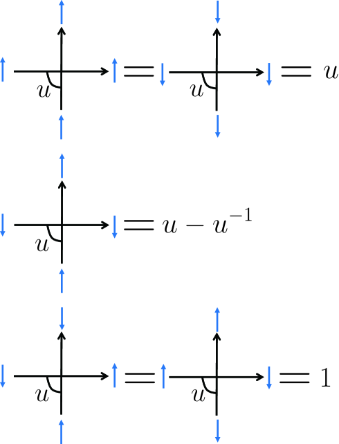
Figure 1: The elements of the $L$-operator (8). The $L$-operator is represented as two crossing arrows. The left and the up arrow represents an auxiliary and a quantum space respectively. The spins on the left and the right around a vertex denote the input and the output of the auxiliary space, and the ones on the bottom and the top denote the input and the output of the quantum space, respectively. For example, $\langle\uparrow|\langle\downarrow|_{j}L(j|u)|\downarrow\rangle|\uparrow\rangle_{j}=1$.

The $L$-operator satisfies the $RLL$ relation

$$R(u,v)(L(n|u)\otimes L(n|v))=(L(n|v)\otimes L(n|u))R(u,v),$$ (9)

where $R(u,v)$ is the $R$-matrix

$$R(u,v)= \left(\begin{array}[]{cccc}f(v,u)&0&0&0\\ 0&g(v,u)&1&0\\ 0&0&g(v,u)&0\\ 0&0&0&f(v,u)\end{array}\right),$$ (14)

$$f(v,u)= \frac{u^{2}}{u^{2}-v^{2}},\ g(v,u)=\frac{uv}{u^{2}-v^{2}}.$$ (15)

From the $RLL$ relation (9), it follows that the monodromy matrix which is defined as a product of $L$ operators

$$T(u)=\prod_{j=1}^{M}L(j|u) =\left(\begin{array}[]{cc}A(u)&B(u)\\ C(u)&D(u)\end{array}\right),$$ (18)

satisfies the $RTT$ relation

$$R(u,v)(T(u)\otimes T(v))=(T(v)\otimes T(u))R(u,v).$$ (19)

From the intertwining relation (19), one immediately finds the transfer matrix

$$\tau(u)=u^{-M}\mathrm{tr}T(u)=u^{-M}(A(u)+D(u)),$$ (20)

forms a commuting family

$$[\tau(u),\tau(v)]=0.$$ (21)

The Markov matrix (2) is constructed from the transfer matrix (20) as

$$\mathcal{M}=\frac{1}{2}\tau^{-1}(1)\frac{\partial}{\partial u}\tau(u)|_{u=1}.$$ (22)

The elements of the $RTT$ relation (19) give the commutation relations between the elements of the transfer matrix $A(u),B(u),C(u)$ and $D(u)$. Some of them are listed as

$$C(u)B(v) =g(u,v)\{A(u)D(v)-A(v)D(u)\},$$ (23)

$$A(u)B(v) =f(u,v)B(v)A(u)+g(v,u)B(u)A(v),$$ (24)

$$D(u)B(v) =f(v,u)B(v)D(u)+g(u,v)B(u)D(v),$$ (25)

$$[B(u),B(v)] =[C(u),C(v)]=0.$$ (26)

The arbitrary $N$-particle state $|\psi(\{u\})\rangle$ (resp. its dual $\langle\psi(\{u\})|$) (not normalized) with $N$ spectral parameters $\{u\}=\{u_{1},u_{2},\dots,u_{N}\}$ is constructed by a multiple action of $B$ (resp. $C$) operator on the vacuum state $|\Omega\rangle$ (respectively, $\langle\Omega|$)

$$|\psi(\{u\})\rangle=\prod_{j=1}^{N}B(u_{j})|\Omega\rangle,\quad\langle\psi(\{u\})|=\langle\Omega|\prod_{j=1}^{N}C(u_{j}).$$ (27)

Utilizing (24), (25), (26) and the action of $A(u)$ and $D(u)$ on the vacuum state

$$A(u)|\Omega\rangle=u^{M}|\Omega\rangle,\ \ \ D(u)|\Omega\rangle=(u-u^{-1})^{M}|\Omega\rangle,$$ (28)

one can show that the state $|\psi(\{u\})\rangle$ is an eigenstate of the transfer matrix (20)

$$\tau(v)|\psi(\{u\})\rangle =\Theta_{N}(v,\{u\})|\psi(\{u\})\rangle,$$ (29)

$$\Theta_{N}(v,\{u\}) =\prod_{j=1}^{N}\frac{u_{j}^{2}}{u_{j}^{2}-v^{2}}+(1-v^{-2})^{M}\prod_{j=1}^{N}\frac{v^{2}}{v^{2}-u_{j}^{2}},$$ (30)

if the spectral parameters $\{u\}=\{u_{1},u_{2},\dots,u_{N}\}$ satisfy the Bethe ansatz equation

$$(1-u_{k}^{-2})^{-M}u_{k}^{-2N}=(-1)^{N-1}\prod_{j=1}^{N}u_{j}^{-2},$$ (31)

for $k=1,2,\cdots,N$. One can also show

$$\langle\psi(\{u\})|\tau(v)=\langle\psi(\{u\})|\Theta_{N}(v,\{u\}),$$ (32)

under the constraint (31). The eigenvalue of the Markov matrix (2) is given by the spectral parameters as

$$\mathcal{M}(\{u\})=\frac{1}{2}\Theta_{N}^{-1}(1,\{u\})\frac{\partial}{\partial v}\Theta_{N}(v,\{u\})|_{v=1}=\sum_{j=1}^{N}\frac{1}{u_{j}^{2}-1}.$$ (33)

The steady state $|S_{N}\rangle$ ($\langle S_{N}|$) corresponds to the eigenstate with zero eigenvalue which is given by setting the spectral parameters as $u_{1}=u_{2}=\cdots=u_{N}=\infty$.

The scalar product, which plays an important role in this paper, has the following determinant form [42]

$$\langle\psi(\{v\})|\psi(\{u\})\rangle=\Bigg{\{}\prod_{N\geq j>k\geq 1}\frac{v_{j}v_{k}}{v_{k}^{2}-v_{j}^{2}}\prod_{N\geq l>n\geq 1}\frac{u_{l}u_{n}}{u_{l}^{2}-u_{n}^{2}}\Bigg{\}}\mathrm{det}_{N}P,$$ (34)

where $P$ is an $N\times N$ matrix with matrix elements

$$P_{jk}=\frac{\Bigg{\{}v_{j}^{M}(u_{k}-u_{k}^{-1})^{M}\Bigg{(}\frac{u_{k}}{v_{j}}\Bigg{)}^{N-1}-u_{k}^{M}(v_{j}-v_{j}^{-1})^{M}\Bigg{(}\frac{u_{k}}{v_{j}}\Bigg{)}^{-N+1}\Bigg{\}}}{\frac{u_{k}}{v_{j}}-\Big{(}\frac{u_{k}}{v_{j}}\Big{)}^{-1}}.$$

Taking $\{v\}=\{u\}$, one gets the determinant representation of the norm

$$\langle\psi(\{u\})|\psi(\{u\})\rangle=\prod_{j=1}^{N}u_{j}^{2(N+M-1)}\prod_{\begin{subarray}{c}l,n=1\atop l\neq n\end{subarray}}^{N}\frac{1}{u_{l}^{2}-u_{n}^{2}}\mathrm{det}_{N}Q,$$ (36)

with $N\times N$ matrix

$$Q_{jk}=\frac{N-1+(M-N+1)u_{j}^{-2}}{1-u_{j}^{-2}}\delta_{jk}-(1-\delta_{jk}).$$ (37)

Note that by use of Sylvester’s determinant theorem, one can reduce the determinant in the above to

$$\mathrm{det}_{N}Q=\prod_{j=1}^{N}\frac{N+(M-N)u_{j}^{-2}}{1-u_{j}^{-2}}\left(1-\sum_{j=1}^{N}\frac{1-u_{j}^{-2}}{N+(M-N)u_{j}^{-2}}\right).$$ (38)

3 Form factors and Overlap

We first formulate the relaxation dynamics of the TASEP to see what we should evaluate. Then we evaluate the form factors and the overlap between the initial state and arbitrary Bethe vector in the determinant and factorized forms. We consider two fundamental initial conditions: the step and alternating initial conditions.

3.1 Formulation of the relaxation dynamics

We formulate the relaxation dynamics of the TASEP by the algebraic Bethe ansatz. The time evolution of the expectation value for the physical quantity $\mathcal{A}$ starting from an initial state $|I_{N}\rangle$ is defined as

$$\langle\mathcal{A}\rangle_{t}=\langle S_{N}|\mathcal{A}e^{\mathcal{M}t}|I_{N}\rangle,$$ (39)

where $\langle S_{N}|$ is the left steady state vector (5). This definition comes from the fact that the TASEP is a stochastic process, and the coefficient $P_{t}(\tau_{1},\dots,\tau_{M})$ of the state vector $|\psi(t)\rangle=e^{\mathcal{M}t}|I_{N}\rangle$ directly gives the probability of being in the state $|\tau_{1},\dots,\tau_{M}\rangle$. We decompose the quantity (39) by inserting the resolution of identity

$$I=\frac{|S_{N}\rangle\langle S_{N}|}{Z_{N}}+\sum_{\alpha}\frac{|\psi_{\alpha}\rangle\langle\psi_{\alpha}|}{\langle\psi_{\alpha}|\psi_{\alpha}\rangle}.$$ (40)

Here $\alpha$ labels arbitrary eigenstates except for the steady state. Then we find the local densities $\langle n_{i}\rangle_{t}=\langle 1-s_{i}\rangle_{t}$ and currents $\langle j_{i}\rangle_{t}=\langle(1-s_{i})s_{i+1}\rangle_{t}$ are respectively given by

$$\langle n_{i}\rangle_{t} =\frac{N}{M}+\sum_{\alpha}\frac{e^{\mathcal{M}_{\alpha}t}(\langle S_{N}|\psi_{\alpha}\rangle-\langle S_{N}|s_{i}|\psi_{\alpha}\rangle)\langle\psi_{\alpha}|I_{N}\rangle}{\langle\psi_{\alpha}|\psi_{\alpha}\rangle},$$ (41)

$$\langle j_{i}\rangle_{t} =\frac{N(M-N)}{M(M-1)}+\sum_{\alpha}\frac{e^{\mathcal{M}_{\alpha}t}(\langle S_{N}|s_{i+1}|\psi_{\alpha}\rangle-\langle S_{N}|s_{i}s_{i+1}|\psi_{\alpha}\rangle)\langle\psi_{\alpha}|I_{N}\rangle}{\langle\psi_{\alpha}|\psi_{\alpha}\rangle}.$$ (42)

In the same way, one can also make the same decomposition for the emptiness formation probability (EFP) $EFP(i,k)_{t}=\langle s_{i}s_{i+1}\cdots s_{i+k-1}\rangle_{t}$, which gives the probability that the sequence of $k$ sites ($i,(i+1),\dots,(i+k-1)$th sites) are all unoccupied

$$EFP(i,k)_{t}$$

$$= \frac{(M-N)!(M-k)!}{M!(M-k-N)!}+\sum_{\alpha}\frac{e^{\mathcal{M}_{\alpha}t}\langle S_{N}|s_{i}s_{i+1}\cdots s_{i+k-1}|\psi_{\alpha}\rangle\langle\psi_{\alpha}|I_{N}\rangle}{\langle\psi_{\alpha}|\psi_{\alpha}\rangle}.$$ (43)

From the expressions of the physical quantities (41), (42) and (43), one notices that what we should evaluate is the norm $\langle\psi_{\alpha}|\psi_{\alpha}\rangle$, the form factors $\langle S_{N}|s_{i}s_{i+1}\cdots s_{i+k-1}|\psi_{\alpha}\rangle$ and the overlap between the initial state and arbitrary Bethe vector $\langle\psi_{\alpha}|I_{N}\rangle$. The norm can be obtained as a limit of the scalar product (34) in the determinant form (36). What remains to be done is the evaluation of the form factors and the overlap.

3.2 Form factors

The form factor for the local operators $s_{i}\cdots s_{i+k-1}$ is explicitly given by the following determinant form

$$\langle S_{N}|s_{i}\cdots s_{i+k-1}|\psi(\{u\})\rangle$$

$$= \prod_{j=1}^{N}(1-u_{j}^{-2})^{k+i-1}\prod_{j=1}^{N}u_{j}^{M+1}\prod_{N\geq l>n\geq 1}\frac{1}{u_{l}^{2}-u_{n}^{2}}\mathrm{det}_{N}V^{(M-k)},$$ (44)

where the $N\times N$ matrix $V$ is written as

$$V_{jl}^{(M-k)}=\sum_{n=0}^{j-1}(-1)^{n}\frac{(M-k)!}{n!(M-k-n)!}u_{l}^{2(j-1-n)},$$ (45)

for $1\leq j\leq N-1$ and

$$V_{Nl}^{(M-k)}=-\sum_{n=N-1}^{M-k}(-1)^{n}\frac{(M-k)!}{n!(M-k-n)!}u_{l}^{-2(n-N+1)}.$$ (46)

Note that the overlap between the steady state and the Bethe vector $\langle S_{N}|\psi\rangle$ is obtained by setting $i=1,k=0$ in (44). We show (44) by applying the approach of [42]. First, let us denote the monodromy matrix constructed from the $(M-k+1)$-th, $\cdots$, $M$-th sites and its matrix elements as

$$T_{k}(u)=\prod_{j=M-k+1}^{M}L(j|u)=\left(\begin{array}[]{cc}A_{k}(u)&B_{k}(u)\\ C_{k}(u)&D_{k}(u)\end{array}\right).$$ (49)

By definition, one has

$$\left(\begin{array}[]{cc}A_{M-k+1}(u)&B_{M-k+1}(u)\\ C_{M-k+1}(u)&D_{M-k+1}(u)\end{array}\right)$$ (52)

$$= \left(\begin{array}[]{cc}A_{M-k}(u)&B_{M-k}(u)\\ C_{M-k}(u)&D_{M-k}(u)\end{array}\right)\left(\begin{array}[]{cc}us_{k}&\sigma_{k}^{-}\\ \sigma_{k}^{+}&uI-u^{-1}s_{k}\end{array}\right),$$ (57)

from which we get

$$B_{M-k+1}(u) =A_{M-k}(u)\sigma_{k}^{-}+B_{M-k}(u)(uI-u^{-1}s_{k}),$$ (58)

$$C_{M-k+1}(u) =C_{M-k}(u)us_{k}+D_{M-k}(u)\sigma_{k}^{+}.$$ (59)

Acting both sides of (58) by $s_{k}$ from the left, and (59) from the right, one has

$$s_{k}B_{M-k+1}(u) =(u-u^{-1})B_{M-k}(u)s_{k},$$ (60)

$$C_{M-k+1}(u)s_{k} =us_{k}C_{M-k}(u).$$ (61)

Utilizing (60) and (61), one can calculate the following generalized form factor as

$$\langle\psi(\{v\})|s_{1}s_{2}\cdots s_{k}|\psi(\{u\})\rangle$$

$$= \langle\Omega|\prod_{j=1}^{N-1}C(v_{j})C(v_{N})s_{1}^{2}s_{2}\cdots s_{k}B(u_{1})\prod_{j=2}^{N}B(u_{j})|\Omega\rangle$$

$$= \langle\Omega|\prod_{j=1}^{N-1}C(v_{j})C(v_{N})s_{1}s_{2}\cdots s_{k}s_{1}B(u_{1})\prod_{j=2}^{N}B(u_{j})|\Omega\rangle$$

$$= \langle\Omega|\prod_{j=1}^{N-1}C(v_{j})v_{N}s_{1}C_{M-1}(v_{N})s_{2}\cdots s_{k}(u_{1}-u_{1}^{-1})B_{M-1}(u_{1})s_{1}\prod_{j=2}^{N}B(u_{j})|\Omega\rangle$$

$$= \prod_{j=1}^{N}v_{j}(u_{j}-u_{j}^{-1})\langle\Omega|\prod_{j=1}^{N}C_{M-1}(v_{j})s_{2}\cdots s_{k}\prod_{j=1}^{N}B_{M-1}(u_{j})|\Omega\rangle$$

$$= \cdots\cdots$$

$$= \prod_{j=1}^{N}v_{j}^{k}(u_{j}-u_{j}^{-1})^{k}\langle\Omega|\prod_{j=1}^{N}C_{M-k}(v_{j})\prod_{j=1}^{N}B_{M-k}(u_{j})|\Omega\rangle.$$ (62)

Utilizing the cyclic property $s_{k}=\tau^{k-j}s_{j}\tau^{j-k},\tau=\tau(1)$ and the action of $\tau$ on the Bethe vector, one gets

$$\langle\psi(\{v\})|s_{i}s_{i+1}\cdots s_{i+k-1}|\psi(\{u\})\rangle$$

$$= \langle\psi(\{v\})|(\tau^{i-1}s_{1}\tau^{1-i})(\tau^{i-1}s_{2}\tau^{1-i})\cdots(\tau^{i-1}s_{k}\tau^{1-i})|\psi(\{u\})\rangle$$

$$= \langle\psi(\{v\})|\tau^{i-1}s_{1}s_{2}\cdots s_{k}\tau^{1-i}|\psi(\{u\})\rangle$$

$$= \Bigg{(}\frac{1-u_{j}^{-2}}{1-v_{j}^{-2}}\Bigg{)}^{i-1}\prod_{j=1}^{N}v_{j}^{k}(u_{j}-u_{j}^{-1})^{k}\langle\Omega|\prod_{j=1}^{N}C_{M-k}(v_{j})\prod_{j=1}^{N}B_{M-k}(u_{j})|\Omega\rangle.$$ (63)

The form factor (44) can be obtained by taking a limit of the generalized form factor (63). First, note that the steady state can be obtained as

$$|S_{N}\rangle =\lim_{\{u\}\to\infty}\prod_{j=1}^{N}\tilde{B}_{M}(u_{j})|\Omega\rangle,$$

$$\langle S_{N}| =\lim_{\{u\}\to\infty}\langle\Omega|\prod_{j=1}^{N}\tilde{C}_{M}(u_{j}),$$ (64)

where $\tilde{B}_{M}(u)=u^{-(M-1)}B_{M}(u)$ and $\tilde{C}_{M}(u)=u^{-(M-1)}C_{M}(u)$. We rewrite the generalized form factor (63) as

$$\langle\Omega|\prod_{j=1}^{N}\tilde{C}_{M}(v_{j})s_{i}s_{i+1}\cdots s_{i+k-1}\prod_{j=1}^{N}\tilde{B}_{M}(u_{j})|\Omega\rangle$$

$$= \Bigg{(}\frac{1-u_{j}^{-2}}{1-v_{j}^{-2}}\Bigg{)}^{i-1}\prod_{j=1}^{N}(1-u_{j}^{-2})^{k}\langle\Omega|\prod_{j=1}^{N}\tilde{C}_{M-k}(v_{j})\prod_{j=1}^{N}\tilde{B}_{M-k}(u_{j})|\Omega\rangle.$$ (65)

Taking $\{v\}\to\infty$, one can show [42]

$$\langle S_{N}|\prod_{j=1}^{N}\tilde{B}_{M}(u_{j})|\Omega\rangle=\prod_{k=1}^{N}u_{k}^{2}\prod_{N\geq l>n\geq 1}\frac{1}{u_{l}^{2}-u_{n}^{2}}\mathrm{det}_{N}V^{(M)},$$ (66)

where

$$V_{jl}^{(M)} =\sum_{n=0}^{j-1}(-1)^{n}\frac{M!}{n!(M-n)!}u_{l}^{2(j-1-n)},\ 1\leq j\leq N-1,$$ (67)

$$V_{Nl}^{(M)} =-\sum_{n=N-1}^{M}(-1)^{n}\frac{M!}{n!(M-n)!}u_{l}^{-2(n-N+1)}.$$ (68)

Taking the limit $\{v\}\to\infty$ in (65) and inserting (66) to the right hand side, we have

$$\langle S_{N}|s_{i}s_{i+1}\cdots s_{i+k-1}\prod_{i=1}^{N}\tilde{B}_{M}(u_{i})|\Omega\rangle$$

$$= \prod_{j=1}^{N}(1-u_{j}^{-2})^{k+i-1}\prod_{j=1}^{N}u_{j}^{2}\prod_{N\geq l>n\geq 1}\frac{1}{u_{l}^{2}-u_{n}^{2}}\mathrm{det}V^{(M-k)}.$$ (69)

Changing from $\tilde{B}_{M}(u)$ to $B_{M}(u)$, one obtains the determinant representation for form factors (44).

3.3 Overlap: Step initial condition

What remains to be done is to evaluate the overlap $\langle\psi_{\alpha}|I_{N}\rangle$ between the initial state and arbitrary Bethe vector. First we consider the step initial condition (see figure  2 (a)) where the half of the system is consecutively occupied by the particles and the other half is empty. By graphical description of the $L$-operator, it is easy to see (figure 3) that the (normalized) initial state $|I_{N}\rangle=|\underbrace{1,\dots,1}_{N},\underbrace{0,\dots,0}_{M-N}\rangle$ is given by $|I_{N}\rangle=B(1)^{N}|\Omega\rangle$ (see [43] for the XXZ spin chain). Note that this initial state is not the eigenstate of the Markov matrix.

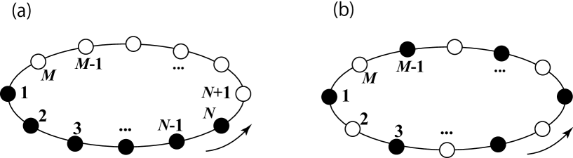
Figure 2: (a) The step initial condition and (b) the alternating initial condition of the TASEP on a ring.

Then we find the overlap $\langle\psi(\{v\})|I_{N}\rangle=\langle\psi(\{v\})|B(1)^{N}|\Omega\rangle=\langle\psi(\{v\})|\psi(\{1\})\rangle$ can be obtained as a limit $\{u\}\to 1$ of the scalar product formula (34). One finds

$$\langle\psi(\{v\})|I_{N}\rangle= \frac{(-1)^{N}}{2^{\frac{N(N+1)}{2}}}\prod_{j=1}^{N}\frac{(v_{j}-v_{j}^{-1})^{M}}{v_{j}^{1-2N}}\prod_{N\geq j>k\geq 1}\frac{1}{v_{j}^{2}-v_{k}^{2}}$$

$$\times\mathrm{det}_{N}\Bigg{(}\frac{1}{(1-v_{j})^{k}}+\frac{1}{(1+v_{j})^{k}}\Bigg{)}.$$ (70)

We can furthermore simplify the determinant as

$$\mathrm{det}_{N}\Bigg{(}\frac{1}{(1-v_{j})^{k}}+\frac{1}{(1+v_{j})^{k}}\Bigg{)}= \mathrm{det}_{N}\Bigg{(}\frac{2}{(1-v_{j}^{2})^{k}}\sum_{l=0\atop l:\mathrm{even}}^{k}\frac{k!}{l!(k-l)!}v_{j}^{l}\Bigg{)}$$

$$= \mathrm{det}_{N}\Bigg{(}\frac{2^{k}}{(1-v_{j}^{2})^{k}}\Bigg{)}$$

$$= \frac{2^{N(N+1)/2}}{\prod_{j=1}^{N}(1-v_{j}^{2})^{N}}\mathrm{det}_{N}((1-v_{j}^{2})^{N-k})$$

$$= \frac{2^{N(N+1)/2}\prod_{N\geq j>k\geq 1}(v_{j}^{2}-v_{k}^{2})}{\prod_{j=1}^{N}(1-v_{j}^{2})^{N}}.$$ (71)

We made column operation in the determinant in the second equality, and used the formula for the Vandermonde determinant

$$\mathrm{det}_{N}(x_{j}^{N-k})=\prod_{N\geq j>k\geq 1}(x_{k}-x_{j}),$$ (72)

in the last equality. Inserting (71) into (70), one gets the following simple form for the case of the step initial condition

$$\langle\psi(\{v\})|I_{N}\rangle=\prod_{j=1}^{N}(v_{j}-v_{j}^{-1})^{M-N}v_{j}^{N-1}.$$ (73)

Note that this form holds for arbitrary filling.

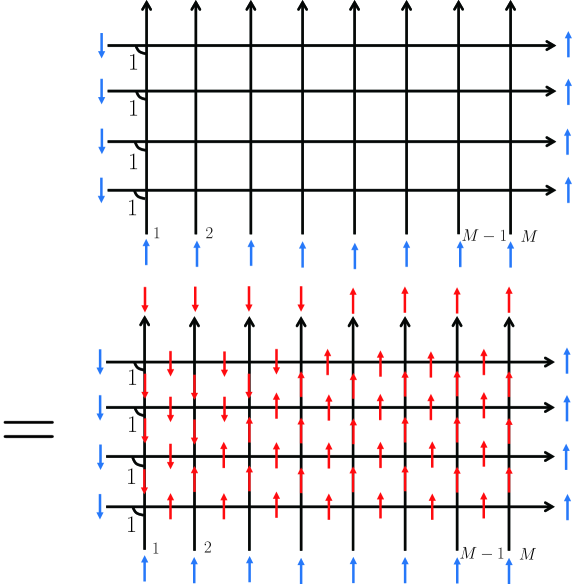
Figure 3: Graphical description of $|I_{N}\rangle=B(1)^{N}|\Omega\rangle$ for the step initial condition. The spins on the bottom line represents the vacuum, and each row corresponds to the $B$ operator. Setting the spectral parameter on the bottom line to be one, one finds the two southwest internal spins freeze since $\langle\uparrow|\langle\downarrow|_{1}L(1|u=1)|\downarrow\rangle|\uparrow\rangle_{1}=1$ and $\langle\downarrow|\langle\uparrow|_{1}L(1|u=1)|\downarrow\rangle|\uparrow\rangle_{1}=0$. Repeating the same game makes one see that all spins freeze. The spins on the top line is the resultant state of the action of $B(1)^{N}$ on the vacuum.

3.4 Overlap: Alternating initial condition

We now evaluate the overlap for the case of the alternating initial condition $|I_{N}\rangle=|1,0,1,0,\dots,1,0\rangle$ (figure 2 (b)), which all odd sites are occupied while all even sites are empty. We consider the half-filling case. We find the following simple form

$$\langle\psi(\{v\})|I_{N}\rangle=\prod_{j=1}^{N}(v_{j}-v_{j}^{-1})\prod_{j,k=1\atop j<k}^{N}(v_{j}^{2}v_{k}^{2}-1).$$ (74)

Let us show (74). For convenience, we use the spin notation (spin up and down states correspond to occupied and empty sites respectively). First, by representing the left hand side of (74) graphically (figure 4), one finds

$$\langle\psi(\{v\})|\downarrow_{1}\uparrow_{2}\downarrow_{3}\uparrow_{4}\cdots\downarrow_{M-1}\uparrow_{M}\rangle= \prod_{j=2}^{N}v_{j}\prod_{j=1}^{N}(v_{j}-v_{j}^{-1})\mathcal{D}_{N}(v_{1},v_{2},\cdots,v_{N}),$$ (75)

$$\mathcal{D}_{N}(v_{1},v_{2},\cdots,v_{N})= \langle\Omega|C(v_{N})\cdots C(v_{2})D(v_{1})|\uparrow_{2}\downarrow_{3}\uparrow_{4}\downarrow_{5}\cdots\downarrow_{M-1}\rangle.$$ (76)

We focus on $\mathcal{D}_{N}(v_{1},v_{2},\cdots,v_{N})$. Again, by graphical representation (figure 5), we note the following recursive relation

$$\mathcal{D}_{N}(\pm 1,v_{2},\cdots,v_{N})=\prod_{j=3}^{N}v_{j}\prod_{j=2}^{N}(v_{j}-v_{j}^{-1})\mathcal{D}_{N-1}(v_{2},\cdots,v_{N}).$$ (77)

Since $\langle\psi(\{v\})|\downarrow_{1}\uparrow_{2}\downarrow_{3}\uparrow_{4}\cdots\downarrow_{M-1}\uparrow_{M}\rangle$ is symmetric with respect to $v_{1},v_{2},\cdots,v_{N}$
$([B(v_{i}),B(v_{j})]=0)$, $\mathcal{D}_{N}(v_{1},v_{2},\cdots,v_{N})$ must be of the form

$$\mathcal{D}_{N}(v_{1},v_{2},\cdots,v_{N})=\prod_{j=2}^{N}v_{j}^{-1}\mathcal{F}_{N}(v_{1},v_{2},\cdots,v_{N}),$$ (78)

where $\mathcal{F}_{N}(v_{1},v_{2},\cdots,v_{N})$ is a symmetric polynomial of $v_{1},v_{2},\cdots,v_{N}$. Utilizing (78), the recursive relation for $\mathcal{D}_{N}(v_{1},v_{2},\cdots,v_{N})$ (77) becomes the one for $\mathcal{F}_{N}(v_{1},v_{2},\cdots,v_{N})$

$$\mathcal{F}_{N}(\pm 1,v_{2},\cdots,v_{N})=\prod_{j=2}^{N}(v_{j}^{2}-1)\mathcal{F}_{N-1}(v_{2},\cdots,v_{N}).$$ (79)

By symmetry, (79) extends to

$$\mathcal{F}_{N}(v_{1},v_{2},\cdots,v_{N})|_{v_{k}=\pm 1}=\prod_{j=1\atop j\neq k}^{N}(v_{j}^{2}-1)\mathcal{F}_{N-1}(v_{1},\cdots,\widehat{v_{k}},\cdots,v_{N}).$$ (80)

One finds

$$\mathcal{F}_{N}(v_{1},v_{2},\cdots,v_{N})=\prod_{j,k=1\atop j<k}^{N}(v_{j}^{2}v_{k}^{2}-1),$$ (81)

solves the recursive relation (80). Combining (75),(78) and (81), one gets the factorized polynomial expression for the overlap (74) between the alternating initial state and arbitrary Bethe vector.

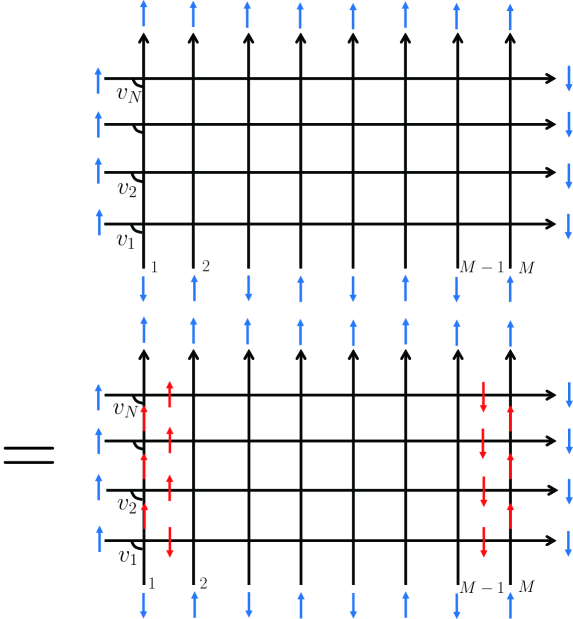
Figure 4: Graphical description of (75) .

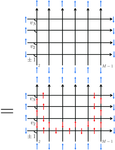
Figure 5: Graphical description of (77) .

4 Excited states

In section 2 and 3, we have formulated the dynamics of the TASEP by the algebraic Bethe ansatz by evaluating ingredients such as the form factors and overlap. In this section, we review the results of the excitation spectrum of the TASEP on a ring [28, 29, 31].

4.1 Algorithm

We review the algorithm of computing the excitation spectrum of the TASEP on a ring. To this end, we make change of variables of the spectral parameters from $u_{j}$ to $Z_{j}$ ($u_{j}^{2}=(Z_{j}+1)/(Z_{j}-1)$) in this section. The Bethe ansatz equation can be rewritten as

$$(1-Z_{k}^{2})^{N}=-2^{M}\prod_{j=1}^{N}\frac{Z_{j}-1}{Z_{j}+1},$$ (82)

for $k=1,2,\dots,N$. The eigenvalue of the Markov matrix becomes

$$\mathcal{M}(\{Z\})=\sum_{j=1}^{N}\frac{Z_{j}-1}{2}.$$ (83)

A simple algorithm was proposed [28] to calculate the roots of the Bethe ansatz equation. Noting the right hand side of (82) does not depend on the index $k$, we define a parameter $u$ as

$$(1-Z_{k}^{2})^{N}=-\mathrm{e}^{\pi u}.$$ (84)

The roots of this equation are

$$Z_{m} =-Z_{N+m}=\sqrt{1-y_{m}},$$ (85)

$$y_{m} =\mathrm{e}^{2\pi(u+i)/M}\mathrm{e}^{4\pi i(m-1)/M},$$ (86)

for $m=1,2,\cdots,N$, and $\{y\}=\{y_{1},y_{2},\dots,y_{N}\}$ satisfy

$$0\leq\mathrm{arg}(y_{1})<\mathrm{arg}(y_{2})<\cdots\mathrm{arg}(y_{N})<2\pi.$$ (87)

It was proposed in [28] that choosing a sequence of quantum numbers $\{c(1),c(2),\dots,c(N)\}$ satisfying $1\leq c(1)<c(2)\cdots<c(N)\leq M$ and determining the parameter $u$ from

$$\mathrm{e}^{\pi u}=2^{M}\prod_{j=1}^{N}\frac{Z_{c(j)}-1}{Z_{c(j)}+1},$$ (88)

self-consistently by numerical iteration, one gets the Bethe roots $\{Z_{c(1)},Z_{c(2)},\dots,Z_{c(N)}\}$.

4.2 Excited states

By numerical calculation, we observe the following types of Bethe roots are the three lowest excited states. We mean a lower-lying excited state by a state whose real part of its corresponding eigenvalue of the Markov matrix is closer to zero. Here, we impose the ansatz that the eigenvalues of the low-lying excited states behave as $\mathrm{ln}(\mathrm{Re}\mathcal{M})=\alpha-\beta\mathrm{ln}M,\beta=3/2$ by the following reasons. Since the lowest excited states believed to be true behave in this way, the exponents $\beta$ for the other excited states should not be $\beta>3/2$ for $M$ large enough since no crossing across the lowest excited states is allowed. Next, by estimating several low-lying excited states by numerical observations for $M\sim 20$ and making finite size scaling analysis of them for large $M$, we find the exponents for all of those states are close to $\beta=3/2$, which is the reason why we impose the ansatz.
$(1)$Type I [28, 29, 31]
The Bethe roots corresponding to the quantum numbers

$$\{c(j)=j\ \mathrm{for}\ j=1,\cdots,N-1,\ c(N)=N+1\},$$ (89)

$$\{c(j)=j+1\ \mathrm{for}\ j=1,\cdots,N-1,\ c(N)=2N\},$$ (90)

give the lowest excited states. The simplest fitting from $M=256,512,1024$ gives $\mathrm{ln}(-\mathcal{M}_{\mathrm{1st}})=1.89793-1.50351\mathrm{ln}M$, which implies the KPZ scaling, i.e. $\mathcal{M}=CM^{-3/2}$ for $M\gg 1$.
$(2)$Type II
The second lowest excited state is given by the quantum number

$$\{c(j)=j+1\ \mathrm{for}\ j=1,\cdots,N-2,\ c(N-1)=N+1,\ c(N)=2N\},$$ (91)

for $M$ large enough. Finite size scaling from $M=256,512,1024$ shows $\mathrm{ln}(-\mathcal{M}_{\mathrm{2nd}})=2.81592-1.505768\mathrm{ln}M$, which shows the KPZ scaling again. This state will be important for the case of the alternating initial condition.
$(3)$Type III
The Bethe roots associated with the following four quantum numbers

$$\{c(j)=j\ \mathrm{for}\ j=1,\cdots,N-1,\ c(N)=N+2\},$$ (92)

$$\{c(j)=j\ \mathrm{for}\ j=1,\cdots,N-2,\ c(N-1)=N,\ c(N)=N+1\},$$ (93)

$$\{c(1)=1,\ c(j)=j+1\ \mathrm{for}\ j=2,\cdots,N-1,\ c(N)=2N\},$$ (94)

$$\{c(j)=j+1\ \mathrm{for}\ j=1,\cdots,N-1,\ c(N)=2N-1\},$$ (95)

give the third lowest excited states. Conducting the finite size scaling from $M=256,512,1024$ shows $\mathrm{ln}(-\mathrm{Re}\mathcal{M}_{\mathrm{3rd}})=2.86964-1.50347\mathrm{ln}M$, which also belongs to the KPZ scaling.

5 Step initial condition

In this and the next section, we examine the relaxation times by studying long time asymptotics of the local current and emptiness formation probability. We consider the step initial condition in this section.
We first analyze the local current. In the long time, the local current behaves as

$$\langle j_{k}\rangle_{t}\rightarrow \frac{N(M-N)}{M(M-1)}+A_{\mathrm{1st}}(j_{k})\mathrm{e}^{\mathcal{M}_{\mathrm{1st}}t}$$

$$+A_{\mathrm{2nd}}(j_{k})\mathrm{e}^{\mathcal{M}_{\mathrm{2nd}}t}+A_{\mathrm{3rd}}(j_{k})\mathrm{e}^{\mathrm{Re}\mathcal{M}_{\mathrm{3rd}}t}\mathrm{cos}(\mathrm{Im}\mathcal{M}_{\mathrm{3rd}}t+\delta_{k})\ \mathrm{as}\ t\rightarrow\infty.$$ (96)

The simplest fitting from $M=256,512,1024$ shows $\mathrm{ln}[A_{\mathrm{1st}}(j_{N})]=0.854409-0.9968579\mathrm{ln}M$, $\mathrm{ln}[-A_{\mathrm{2nd}}(j_{N})]=1.1875099-0.9838921\mathrm{ln}M$ and $\mathrm{ln}[|A_{\mathrm{3rd}}(j_{N})|]=2.20350-0.98345\mathrm{ln}M$ from which one concludes $A_{\mathrm{1st}}(j_{N})\propto M^{-1}$, $A_{\mathrm{2nd}}(j_{N})\propto M^{-1}$ and $|A_{\mathrm{3rd}}(j_{N})|\propto M^{-1}$. Especially, $A_{\mathrm{1st}}(j_{N})\propto M^{-1}$ means that $A_{\mathrm{1st}}(j_{N})\neq 0$ as long as the total number of sites $M$ is finite, confirming the relaxation time of the step initial condition $\tau_{\mathrm{step}}$ is determined by the lowest eigenvalue of the Markov matrix which shows the KPZ scaling $\tau_{\mathrm{step}}=-\mathrm{Re}(1/\mathcal{M}_{\mathrm{1st}})\propto M^{3/2}$.

We can also examine the asymptotic amplitudes of the EFP.

$$EFP(i,k)_{t}\rightarrow\frac{(M-N)!(M-k)!}{M!(M-k-N)!}+A(EFP(i,k))\mathrm{e}^{\mathcal{M}_{\mathrm{1st}}t}\ \mathrm{as}\ t\rightarrow\infty.$$ (97)

Table 2 is the results of the finite size scaling of the asymptotic amplitudes. One observes $A(EFP(i,k))\propto M^{-\alpha_{k}}$, and $\alpha_{k}$ becomes smaller as the length $k$ becomes longer.

Table 1: Table of the asymptotic amplitudes vs total number of sites (step initial condition).

$(i,k)$	$\mathrm{ln}[-A(EFP(i,k))]$
$(N,1)$	$1.93798-1.49332\mathrm{ln}M$
$(N-1,2)$	$1.35223-1.05592\mathrm{ln}M$
$(N-2,3)$	$1.42851-1.01683\mathrm{ln}M$
$(N-3,4)$	$1.22155-0.99148\mathrm{ln}M$
$(N-4,5)$	$0.84935-0.96772\mathrm{ln}M$
$(N-5,6)$	$0.36629-0.94290\mathrm{ln}M$
$(N-6,7)$	$-0.19885-0.91613\mathrm{ln}M$
$(N-7,8)$	$-0.82903-0.88705\mathrm{ln}M$
$(N-8,9)$	$-1.51332-0.85549\mathrm{ln}M$
$(N-9,10)$	$-2.24430-0.82136\mathrm{ln}M$

6 Alternating initial condition

Next we study the alternating initial condition. Surprisingly, we find that the asymptotic amplitudes of the local currents associated with the lowest (Type I) and the third lowest (Type III) excited states vanish. This can be shown as follows. Rewriting the overlap (74) in terms of the spectral parameters $Z_{c(j)}$ in section 4, the following terms

$$\prod_{j,k=1\atop j<k}^{N}(Z_{c(j)}+Z_{c(k)}),$$ (98)

appear. Let us take a look at one of the excited states of Type I $\{c(j)=j\ \mathrm{for}\ j=1,\cdots,N-1,\ c(N)=N+1\}$, for example. There exists a term $Z_{1}+Z_{N+1}$ since $c(1)=1,c(N)=N+1$. However, this term is equal to zero since it is one of the cases of $Z_{k}+Z_{N+k}=0$ (85). Not only the excited states of Type I but also for a large number of low-lying excited states, Type III, for example, have terms $Z_{k}+Z_{N+k}$ which eventually become zero. These states do not make any contributions to the relaxation dynamics. Instead, we find that the second lowest excited state (Type II) determines the relaxation time $\tau_{\mathrm{alt}}$ for the case of the alternating initial condition. Note that the eigenvalue corresponding to the second lowest excited state obeys the KPZ scaling $\tau_{\mathrm{alt}}=-\mathrm{Re}(1/\mathcal{M}_{\mathrm{2nd}})\propto M^{3/2}$ (see Section 4.2). Thus the local current asymptotically behaves as

$$\langle j_{k}\rangle_{t} \rightarrow\frac{N(M-N)}{M(M-1)}+B_{\mathrm{2nd}}(j_{k})\mathrm{e}^{\mathcal{M}_{\mathrm{2nd}}t}\ \mathrm{as}\ t\to\infty.$$ (99)

The fitting from $M=256,512,1024$ shows $\mathrm{ln}[B_{\mathrm{2nd}}(j_{k})]=0.23825-0.99819\mathrm{ln}M$ for both $k$ odd (initially occupied) and even (initially empty). From this, one concludes $B_{\mathrm{2nd}}(j_{k})\propto M^{-1}$, which is the same with the step initial condition.

Next, we analyze the EFP. Again, we find the lowest and third lowest excited states do not contribute.

$$EFP(i,k)_{t}\rightarrow\frac{(M-N)!(M-k)!}{M!(M-k-N)!}+B(EFP(i,k))\mathrm{e}^{\mathcal{M}_{\mathrm{2nd}}t}\ \mathrm{as}\ t\rightarrow\infty.$$ (100)

Table 2: Table of the asymptotic amplitudes vs total number of sites (alternating initial condition).

$(i,k)$	$\mathrm{ln}[-B(EFP(i,k))]$
$(1,2)$	$0.23825-0.99819\mathrm{ln}M$
$(1,3)$	$0.63787-0.99736\mathrm{ln}M$
$(1,4)$	$0.60321-0.99248\mathrm{ln}M$
$(1,5)$	$0.35850-0.98402\mathrm{ln}M$
$(1,6)$	$-0.01838-0.97179\mathrm{ln}M$
$(1,7)$	$-0.49028-0.95602\mathrm{ln}M$
$(1,8)$	$-1.03631-0.93678\mathrm{ln}M$
$(1,9)$	$-1.64345-0.91417\mathrm{ln}M$
$(1,10)$	$-2.30316-0.88825\mathrm{ln}M$

One observes $B(EFP(i,k))\propto M^{-\beta_{k}}$, and $\beta_{k}$ becomes smaller as the length $k$ becomes longer. This behavior is similar with the step initial condition.

7 Conclusion

In this paper, we studied the long time asymptotics of the relaxation dynamics of the totally asymmetric simple exclusion process. We examined the local currents by the algebraic Bethe ansatz method. By evaluating the asymptotic amplitudes, we find the relaxation times starting from the step and alternating initial conditions are governed by different eigenvalues of the Markov matrix. The relaxation time of the step initial condition $\tau_{\mathrm{step}}$ is given by the nonzero eigenvalue of the Markov matrix with the first largest real part $\mathcal{M}_{\mathrm{1st}}$ as $\tau_{\mathrm{step}}=-\mathrm{Re}(1/\mathcal{M}_{\mathrm{1st}})$. On the other hand, the relaxation time of the alternating initial condition $\tau_{\mathrm{alt}}$ is given by the nonzero eigenvalue of the Markov matrix with the second largest real part $\mathcal{M}_{\mathrm{2nd}}$ as $\tau_{\mathrm{alt}}=-\mathrm{Re}(1/\mathcal{M}_{\mathrm{2nd}})$ for large number of total sites. The difference between the step and alternating initial conditions is observed in another context: the current fluctuation. The GUE Tracy-Widom distribution appears for the case of the step initial condition [17]. On the other hand, the current fluctuation for the alternating initial condition is described by the GOE Tracy-Widom distribution [18, 19]. Our results of the relaxation times is another aspect of the difference between the step and alternating initial conditions.

In this paper, we examined the dynamics of the TASEP by use of the algebraic Bethe ansatz method. It is interesting to study other correlation functions and extend to other cases like open boundary, for example. The recent advances [44, 45] might be helpful for this case. It would also be valuable to study the link with the random matrix theory. The case examined in this paper is when the time is large enough, while the case obtained by the random matrix theory is when the time and the size of the system are comparable. These two results are considered to be supplementary to each other, and unifying the results by the Bethe ansatz would be an interesting problem.

References

References

• [1] Derrida B 1998 Phys. Rep. 301 65
• [2] SchΓΌtz G M 2000 Exactly Solvable Models for Many-Body Systems Far from Equilibrium Phase Transitions and Critical Phenomena vol 19 (London: Academic)
• [3] Spitzer F 1970 Adv. in Math. 5 246
• [4] Liggett T M 1999 Stochastic Interacting Systems: Contact, Vote, and Exclusion Processes (New York: Springer-Verlag)
• [5] Spohn H 1991 Large Scale Dynamics of Interacting Particles (New York: Springer-Verlag)
• [6] Macdonald C T, Gibbs J H and Pipkin A.C 1968 Biopolymers 6 1
• [7] Schadschneider A 2001 Physica A 285 101
• [8] Schadschneider A, Chowdhury D and Nishinari K 2010 Stochastic Transport in Complex Systems: From Molecules to Vehicles (Amsterdam: Elsevier Science)
• [9] Karzig T and von Oppen F 2010 Phys. Rev. B 81 045317
• [10] Derrida B, Evans M R, Hakim V and Pasquier V 1993 J. Phys. A: Math. Gen. 26 1493
• [11] SchΓΌtz G M and Domany E 1993 J. Stat. Phys. 72 277
• [12] Sandow S 1994 Phys. Rev. E 50 2660
• [13] Sasamoto T 1999 J. Phys. A: Math. Gen. 32 7109
• [14] Blythe R A, Evans M R, Colaiori F and Essler F H L 2000 J. Phys. A: Math. Gen. 33 2313
• [15] Uchiyama M, Sasamoto T and Wadati M 2004 J. Phys. A: Math. Gen. 37 4985
• [16] Krug J 1991 Phys. Rev. Lett. 67 1882
• [17] Johansson K 2000 Comm. Math. Phys. 209 437
• [18] Baik J and Rains E M 2000 J. Stat. Phys. 100 523
• [19] PrΓ€hofer M and Spohn H 2002 In and out of equilibrium Progress in Probability vol 51 ed V Sidoravicius (Boston: Birkhauser) p 185
• [20] Nagao T and Sasamoto T 2004 Nucl. Phys. B 699 487
• [21] Rakos A and SchΓΌtz G M 2005 J. Stat. Phys. 118 511
• [22] Borodin A, Ferrari P, PrΓ€hofer M and Sasamoto T 2007 J. Stat. Phys. 129 1055
• [23] Imamura T and Sasamoto T 2007 J. Stat. Phys. 128 799
• [24] Tracy C and Widom H J. Math. Phys. 50 095204
• [25] Dhar D 1987 Phase Transitions 9 51.
• [26] Gwa L H and Spohn H 1992 Phys. Rev. A 46 844
• [27] Kim D 1995 Phys. Rev. E 52 3512
• [28] Golinelli O and Mallick K 2004 J. Phys. A: Math. Gen. 37 3321
• [29] Golinelli O and Mallick K 2005 J. Phys. A: Math. Gen. 38 1419
• [30] de Gier J and Essler F H L 2005 Phys. Rev. Lett. 95 240601
• [31] de Gier J and Essler F H L 2006 J. Stat. Mech. P12011
• [32] Arita C, Kuniba A, Sakai K and Sawabe T 2009 J. Phys. A: Math. Theor. 42 345002
• [33] de Gier J, Finn C and Sorrell M 2011 J. Phys. A: Math. Theor. 44 405002
• [34] Derrida B and Lebowitz J L 1998 Phys. Rev. Lett. 80 209
• [35] Prolhac S and Mallick K 2008 J. Phys. A: Math. Theor. 41 175002
• [36] Prolhac S and Mallick K 2009 J. Phys. A: Math. Theor. 42 175001
• [37] Prolhac S 2010 J. Phys. A: Math. Theor. 43 105002
• [38] de Gier J and Essler F H L 2011 Phys. Rev. Lett. 107 010602
• [39] Motegi K, Sakai K and Sato J 2012 Phys. Rev. E 85 042105
• [40] Takhtajan L A and Faddeev L D 1979 Russ. Math. Surveys 34 11
• [41] Korepin V E, Bogoliubov N M and Izergin A G 1993 Quantum Inverse Scattering Method and Correlation functions (Cambridge: Cambridge University)
• [42] Bogoliubov N M 2009 SIGMA 5 052
• [43] Mossel J and Caux J S 2010 New J. Phys. 12 055028
• [44] Crampe N, Ragoucy E and Simon D 2010 J. Stat. Mech. P11038
• [45] Crampe N, Ragoucy E and Simon D 2011 J. Phys. A: Math Theor. 44 405003