Quantum Heat Engine in the relativistic limit: The case of a Dirac-particle

Abstract

We studied the efficiency of two different schemes for a quantum heat engine, by considering a single Dirac particle trapped in a one-dimensional potential well as the ”working substance”. The first scheme is a cycle, composed of two adiabatic and two iso-energetic reversible trajectories in configuration space. The trajectories are driven by a quasi-static deformation of the potential well due to an external applied force. The second scheme is a variant of the former, where iso-energetic trajectories are replaced by isothermal ones, along which the system is in contact with macroscopic thermostats. This second scheme constitutes a quantum analogue of the classical Carnot cycle. Our expressions, as obtained from the Dirac single-particle spectrum, converge in the non-relativistic limit to some of the existing results in the literature for the Schrödinger spectrum.

I Introduction

A classical heat engine consists of a cyclic sequence of reversible transformations over a ”working substance”, typically a macroscopic mass of fluid enclosed in a cylinder with a mobile piston at one end Fermi (1936); Callen (1985). The two most famous examples are the Otto and Carnot cycles. In particular, the classical Carnot cycle comprises four stages, two isothermal and two adiabatic (iso-entropic) ones. Ideal quasi-static and reversible conditions are achieved by assuming that an external force, which differs only infinitesimally from the force exerted by the internal pressure of the fluid, is applied to the piston in order to let it move extremely slowlyFermi (1936); Callen (1985). On the other hand, the isothermal trajectories are performed by bringing the fluid contained by the cylinder into thermal equilibrium with external reservoirs at temperatures $T_{C}<T_{H}$, respectively.

A quantum analogue of a heat engine involves a sequence of transformations (trajectories) in Hilbert’s space, where the ”working substance” is of quantum mechanical natureBender et al. (2002, 2000); Wang et al. (2011); Wang and He (2012); Quan et al. (2006); Arnaud et al. (2002); Latifah and Purwanto (2011); Quan et al. (2007, 2005). One of the simplest conceptual realizations of this idea is a system composed by a single-particle trapped in a one-dimensional infinite potential well Wang and He (2012); Wang et al. (2011); Bender et al. (2002, 2000); Latifah and Purwanto (2011). The different trajectories are driven by a quasi-static deformation of the potential well, due to the application of an external force. Two different schemes of this process have been discussed in the literature, in the context of a non-relativistic particle whose energy eigenstates are determined by the Schrödinger spectrum Bender et al. (2002, 2000); Quan et al. (2007). In this paper, we shall revisit these approaches, and we will study the performance of the corresponding heat engine for a single Dirac particle. Since Dirac’s equation describes the spectra of relativistic particles, results obtained for this case should reduce to the corresponding ones from Schrödinger’s equation in the non-relativistic limit. As we shall discuss below, the transition between the relativistic and non-relativistic regimes is determined by the ratio $\lambda/L$, with $\lambda=2\pi\hbar/mc$ the Compton wavelength of the particle, and $L$ the width of the potential well. The non-relativistic limit corresponds to the regime where $\lambda/L\ll 1$, while evidence of the underlying relativistic nature of the spectrum manifests in terms of finite corrections in powers of $\lambda/L$. Another limit of theoretical interest is the ”ultra-relativistic” case of massless Dirac particles, where $\lambda/L\rightarrow\infty$. An important realization of this former case in solid state systems is provided by conduction electrons in the vicinity of the so called Dirac point in graphene Peres (2010); Castro et al. (2009); Muñoz et al. (2010); Muñoz (2012).

II A Dirac particle trapped in a one-dimensional infinite potential well

The problem of a Dirac particle in the presence of a one-dimensional, finite potential well $V(x)$ is expressed by the Dirac Hamiltonian operator Thaller (1956); Bjorken and Drell (1964),

$$\hat{H}=-i\hbar c\bm{\alpha}\cdot\nabla+mc^{2}\hat{\beta}+V(x)\hat{\mathbf{1}}.$$ (1)

Here,

$$\hat{\alpha}_{i}=\left(\begin{array}[]{cc}0&\hat{\sigma}_{i}\\ \hat{\sigma}_{i}&0\end{array}\right), \hat{\beta}=\left(\begin{array}[]{cc}I&0\\ 0&-I\end{array}\right)$$ (6)

are Dirac matrices in 4 dimensions, with $\hat{\sigma}_{i}$ the Pauli matrices. The domain of this operator is ${\mathcal{D}}(\hat{H})=\mathcal{H}$, with ${\mathcal{H}}=L^{2}(\mathbb{R})\oplus L^{2}(\mathbb{R})\oplus L^{2}(\mathbb{R})\oplus L^{2}(\mathbb{R})\equiv L^{2}(\mathbb{R},\mathbb{C}^{4})$ the Hilbert space of (complex-valued) 4-component spinors $\hat{\psi}(x)=(\phi_{1},\phi_{2},\chi_{3},\chi_{4})$, where each component $\phi_{i},\chi_{j}\in L^{2}(\mathbb{R})$ is therefore a square-integrable function in the unbounded domain $\mathbb{R}$. For a finite potential well, of the form $V(x)=V_{0}\Theta(|x|-L/2)$ with $0<V_{0}<\infty$, it is well discussed in the classical literature Sakurai (1967); Thaller (1956) that confinement is possible only if the energy $E$ of the particle inside the well is in the interval $|E-V_{0}|<mc^{2}$, which corresponds to an exponentially vanishing probability current outside ($x>L/2$ or $x<-L/2$) the confining region. If, on the contrary, the energy is such that $E-V_{0}<-mc^{2}$, then so-called Klein tunneling occurs: The particle can tunnel through the barrier with a finite probability current, but paradoxically with an antiparticle character. This behavior and some of its consequences is denominated Klein’s paradoxSakurai (1967); Thaller (1956); Bjorken and Drell (1964). We remark that this effect occurs when attempting to confine the particle with a finite potential well.

The mathematical and physical pictures are rather different when considering the singular limit of an infinite potential well,

$$V(x)=\left\{\begin{array}[]{cc}0\,,&|x|\leq L/2\\ +\infty\,,&|x|>L/2\end{array}\right..$$ (9)

The singular character of the infinite potential well, exactly as in the more familiar Schrödinger case Carreau et al. (1990), requires a different mathematical statement of the problem: one needs to define a self-adjoint extension Thaller (1956); Carreau et al. (1990); Alonso et al. (1997); Alberto et al. (1996) of the free particle Hamiltonian

$$\hat{H}_{0}=-i\hbar c\bm{\alpha}\cdot\nabla+mc^{2}\hat{\beta},$$ (10)

whose domain $\mathcal{D}(\hat{H}_{0})\subset\mathcal{H}_{\Omega}$ is a dense proper subset of the Hilbert space $\mathcal{H}_{\Omega}=L^{2}(\Omega)\oplus L^{2}(\Omega)\oplus L^{2}(\Omega)\oplus L^{2}(\Omega)\equiv L^{2}(\Omega,\mathbb{C}^{4})$ of square-integrable (complex-valued) 4-component spinors in the closed interval $x\in\Omega=[-L/2,L/2]$. In general, the domain of $\hat{H}_{0}$ and its adjoint $\hat{H}_{0}^{\dagger}$ verify $\mathcal{D}(\hat{H}_{0})\subseteq\mathcal{D}(\hat{H}_{0}^{\dagger})$ Thaller (1956). However, physics requires for $\hat{H}_{0}$ to be self-adjoint. The self-adjoint extension is obtained by imposing appropriate boundary conditions Thaller (1956); Carreau et al. (1990); Alonso et al. (1997); Alberto et al. (1996) on the spinors at the boundary $\partial\Omega$ of the finite domain $\Omega$, as discussed in detail in Appendix A. In particular, the condition of simultaneous vanishing of the four components of the spinor at the boundaries $x=\pm L/2$ is not compatible with self-adjointness and, moreover, leads to the trivial null solution $\hat{\psi}(x)=0$ $\forall x\in\Omega$. Instead, as shown in Appendix A, the mathematical condition for self-adjointness corresponds to a vanishing probability current at the boundary $\partial\Omega$ of the domain $\Omega=[-L/2,L/2]$, $j^{1}(x=\pm L/2)=0$, with $j^{1}(x)=c\hat{\psi}^{\dagger}(x)\hat{\alpha}_{1}\hat{\psi}(x)$. The physical interpretation of this mathematical condition is rather obvious: the particle is indeed ”trapped” inside the infinite potential well, since there is a zero probability current through the boundary walls. This approach has been used in the past, for instance, to model confinement of hadrons in finite regions of space Chodos et al. (1974a, b). Summarizing, the eigenvalue problem for the self-adjoint extension of the free Dirac Hamiltonian Eq.(10) representing particles ”trapped” inside the infinite potential well is given by

$$\hat{H}_{0}\hat{\psi}=E\hat{\psi},$$ (11)

subject to the boundary conditions

$$j^{1}(x=\pm L/2)=0.$$ (12)

As shown explicitly in Appendix A, there is a whole family of eigenfunctions of Eq.(11) in $\Omega=[-L/2,L/2]$, satisfying the boundary conditions Eq.(12). This has been investigated for instance in Alonso et al. (1997); Alberto et al. (1996).

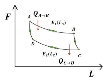
Figure 1: (Color online)Pictorial description of the Force versus size of the potential well, for the Isoenergetic cycle described in the text.

On the other hand, a fundamental discrete symmetry of the Dirac Hamiltonian is its invariance under parity Sakurai (1967); Bjorken and Drell (1964); Thaller (1956) ($\hat{P}$: $x\rightarrow-x$, $p_{x}\rightarrow-p_{x}$), $[\hat{H}_{0},\hat{P}]=0$, which corresponds to a mirror spatial reflection by leaving the spin direction invariant. It is straightforward to show that under parity, the spinor transforms as Bjorken and Drell (1964); Sakurai (1967); Thaller (1956) $\hat{P}\hat{\psi}(x)\hat{P}^{-1}=e^{i\phi}\hat{\beta}\hat{\psi}(-x)$. On the other hand, the probability density defined as $\rho(x)=\hat{\psi}^{\dagger}(x)\hat{\psi}(x)=c^{-1}j^{0}(x)$ is the time-component of the Lorentz 4-vector $j^{\mu}=c\bar{\psi}(x)\gamma^{\mu}\hat{\psi}(x)$, with $\bar{\psi}(x)\equiv\gamma^{0}\hat{\psi}^{\dagger}(x)$. Here, the explicit covariant notation $\gamma^{i}=\hat{\beta}\hat{\alpha}_{i}$ (i=1,2,3), $\gamma^{0}=\hat{\beta}$ was invoked. Under parity, the space components of a Lorentz 4-vector invert sign ($j^{i}\rightarrow-j^{i}$, i = 1,2,3), whereas the time component $j^{0}$ remains invariant Bjorken and Drell (1964); Sakurai (1967); Thaller (1956), and hence $\rho(-x)=\rho(x)$. For the physically acceptable eigenfunctions of the self-adjoint extension of the Dirac Hamiltonian Eqs.(11),(12), we thus demand that this symmetry is satisfied $\forall x\in\Omega=[-L/2,L/2]$. As shown in detail in Appendix A, this leads to a quantization of the wavenumbers, $k\equiv k_{n}=n\pi/L$, for $n\in\mathbb{N}$. The spinor-eigenfunctions obtained from this analysis are

$$\hat{\psi}_{n}(x)=A\left(\begin{array}[]{c}\sin(n\pi(x-L/2)/L)\\ 0\\ 0\\ -\frac{in\lambda/(2L)}{\sqrt{1+n^{2}(\lambda/2L)^{2}}}\cos(n\pi(x-L/2)/L)\end{array}\right),$$ (17)

with associated discrete energy eigenvalues,

$$E_{n}^{D}(L)=mc^{2}\left(\sqrt{1+\left(n\lambda/2L\right)^{2}}-1\right).$$ (18)

Here, we have subtracted the rest energy, and $\lambda=2\pi\hbar/(mc)$ is the Compton wavelength. The positive sign corresponds to the particle solution Bjorken and Drell (1964).

The spectrum predicted by Eq.(18) , as well as the probability density obtained from Eq.(17), can be compared with the corresponding Schrödinger problem, whose eigenvalues are given by

$$E_{n}^{S}(L)=\frac{n^{2}\pi^{2}\hbar^{2}}{2mL^{2}}.$$ (19)

Here, a single eigenvalue for the energy is obtained and, moreover, it scales as $n^{2}$, in contrast with the Dirac particle case where a richer scaling with $n$ is observed. In particular, in the regime $\lambda/L\ll 1$, we have:

$$E_{n}^{D}(L)\rightarrow\frac{mc^{2}}{2}\left(n\lambda/2L\right)^{2}=E_{n}^{S}(L),$$ (20)

corresponding to the non-relativistic limit. Beyond this regime, relativistic corrections depending on the finite ratio $\lambda/L$ are observed.

Regarding the probability density, in the corresponding Schrödinger problem one obtains $\rho^{S}(x)\propto\sin^{2}(n\pi(x-L/2)/L)$ for $x\in\Omega=[-L/2,L/2]$. It is straightforward to verify that, in the non-relativistic limit $\lambda/L\ll 1$, the ”small” component of the spinor in Eq.(17) becomes negligible, and thus the probability density converges to the Schrödinger case, $\rho(x)=\hat{\psi}^{\dagger}(x)\hat{\psi}(x)\rightarrow|A|^{2}\sin^{2}(n\pi(x-L/2)/L)$.

Another interesting limit of Eq.(18) corresponds to a massless Dirac particle with $\lambda\rightarrow\infty$, where the spectrum reduces to the expression

$$\left.E_{n}^{D}(L)\right|_{m=0}=\frac{n\pi\hbar c}{L}.$$ (21)

This situation may be of interest in graphene systems, where conduction electrons in the vicinity of the so called Dirac point can be described as effective massless chiral particles, satisfying Dirac’s equation in two dimensionsPeres (2010); Castro et al. (2009); Muñoz et al. (2010); Muñoz (2012).

III A single-particle Quantum heat Engine

As the ”working substance” for a quantum heat engine, let us consider a statistical ensemble of copies of a single-particle system, where each copy may be in any of the possible different energy eigenstates. We therefore say that the single-particle system is in a statistically mixed quantum statevon Neumann (1955). The corresponding density matrix operator is $\hat{\rho}=\sum_{n}p_{n}(L)|\psi_{n}(L)\rangle\langle\psi_{n}(L)|$, with $|\psi_{n}(L)\rangle$ an eigenstate of the single-particle Hamiltonian Eq.(10), corresponding to the spinors defined by Eq.(17). This density matrix operator is stationary, since in the absence of an external perturbationvon Neumann (1955) $i\hbar\partial_{t}\hat{\rho}=[\hat{H},\hat{\rho}]=0$. Here, the coefficient $0\leq p_{n}(L)\leq 1$ represents the probability for the system, within the statistical ensemble, to be in the particular state $|\psi_{n}(L)\rangle$. Therefore, the $\{p_{n}(L)\}$ satisfy the normalization condition

$${\rm{Tr}}\hat{\rho}=\sum_{n}p_{n}(L)=1.$$ (22)

In the context of Quantum Statistical Mechanics, entropy is defined according to von Neumann von Neumann (1955); Tolman (1938) as $S=-k_{B}{\rm{Tr}}\hat{\rho}\ln\hat{\rho}$. Since in the energy eigenbasis the equilibrium density matrix operator is diagonal, the entropy reduces to the explicit expression

$$S(L)=-k_{B}\sum_{n}p_{n}(L)\ln\left(p_{n}(L)\right).$$ (23)

In our notation, we emphasize explicitly the dependence of the energy eigenstates $\{|\psi_{n}(L)\rangle\}$, as well as the probability coefficients $\{p_{n}(L)\}$, on the width of the potential well $L$.

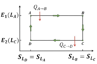
Figure 2: (Color online)Pictorial description of the Energy versus Entropy (von Neumann) for the Isoenergetic cycle.

The ensemble-average energy of the quantum single-particle system is

$$E\equiv\langle\hat{H}\rangle={\rm{Tr}}(\hat{\rho}\hat{H})=\sum_{n}p_{n}(L)E_{n}(L).$$ (24)

For the statistical ensemble just defined, we conceive two different schemes for a quantum analogue of a thermodynamic heat engine. The first one, that we shall refer to as the Isoenergetic cycle, consists on four stages of reversible trajectories: two iso-entropic and two iso-energetic ones, as originally proposed by Bender et al.Bender et al. (2002, 2000) in the context of a Schrödinger particle. During the iso-energetic trajectories, the ensemble-average energy Eq.(24) is conserved, while during the iso-entropic ones, the von Neumann entropy defined by Eq.(23) remains constant. We distinguish this first scheme from the quantum Carnot cycle to be discussed next, where the iso-energetic trajectories in Hilbert’s space are replaced by isothermal processes. During these stages, the system is brought into thermal equilibrium with macroscopic reservoirs at temperatures $T_{C}\leq T_{H}$, respectively.

IV The Isoenergetic Cycle

The Isoenergetic cycle, a scheme for a quantum heat-engine originally proposed by Bender et al. Bender et al. (2002, 2000) in the context of a single Schrödinger particle, is composed by two isoentropic and two isoenergetic trajectories. In particular, during the isoenergetic trajectories, the ”working substance” must exchange energy with an energy reservoir Wang et al. (2011); Wang and He (2012). A possible practical realization of this cycle was proposed in the context of non-relativistic particles in Ref.Wang et al. (2011), where the working substance exchanges energy with single-mode radiation in a cavity, which acts as an energy reservoir.

The system trajectories in Hilbert’s space are assumed to be driven by reversible quasi-static processes, in which the walls of the potential well are deformed ”very slowly” by an applied external force, such that the distance $L$ is modified accordingly. Along these trajectories, the total change in the ensemble average energy of the system is given by

$$dE = \sum_{n}p_{n}(L)dE_{n}(L)+\sum_{n}dp_{n}(L)E_{n}(L)$$ (25)

$$= \left(\delta E\right)_{\{p_{n}(L)\}=cnt.}+\left(\delta E\right)_{\{E_{n}(L)\}=cnt.}$$

The first term in Eq.(25) represents the total energy change due to an iso-entropic process, whereas the second term represents a trajectory where the energy spectrum remains rigid.

Let us consider first the iso-entropic process, where $\{p_{n}(L)\}=cnt$. We remark that this represents a strong sufficient condition for the entropy to remain constant along the trajectory, but is not a necessary onenot (a). Under quasi-static conditions, the external force driving the change in the width of the potential well is equal to the internal ”pressure” of the one-dimensional system, $F=-(\partial E/\partial L)_{S}$. Therefore, the work performed by the system against the external force, when the width of the potential well expands from $L=L_{1}$ to $L=L_{2}$, is given by

$$W_{1\rightarrow 2} = \int_{L_{1}}^{L_{2}}dL\left(\frac{\partial E}{\partial L}\right)_{\{p_{n}(L)\}=\{p_{n}(L_{1})\}=cnt.}$$ (26)

$$= \sum_{n=1}^{\infty}p_{n}(L_{1})\left[E_{n}(L_{2})-E_{n}(L_{1})\right].$$

For the case of a Dirac particle, the work performed under iso-entropic conditions is given after Eq.(26) and Eq.(18) by

$$W_{1\rightarrow 2} = mc^{2}\sum_{n=1}^{\infty}p_{n}(L_{1})\left(\sqrt{1+\left(n\lambda/2L_{2}\right)^{2}}\right.$$ (27)

$$\left.-\sqrt{1+\left(n\lambda/2L_{1}\right)^{2}}\right).$$

Notice that our sign convention is such that, for an expansion process $L_{2}>L_{1}$, the work performed by the system is negativeCallen (1985), indicating that the ensemble-averaged energy is decreasing during expansion, as in a classical ideal gas.

Let us now consider an iso-energetic process, that is, a trajectory in Hilbert space defined by the equation $dE=0$. The solution to this equation, for $L\in[L_{1},L_{2}]$, is given by the path

$$\sum_{n=1}^{\infty}p_{n}(L)E_{n}(L)=\sum_{n=1}^{\infty}p_{n}(L_{1})E_{n}(L_{1}),$$ (28)

along with the normalization condition Eq.(22). Clearly, by definition an iso-energetic process satisfies

$$dE=\delta W_{1\rightarrow 2}+\delta Q_{1\rightarrow 2}=0,$$ (29)

with $\delta W_{1\rightarrow 2}\equiv\left(\delta E\right)_{\{p_{n}(L)\}=cnt.}$ and $\delta Q_{1\rightarrow 2}\equiv\left(\delta E\right)_{\{E_{n}(L)\}=cnt.}$. In the former equation, the integral along the trajectory $L_{1}\rightarrow L_{2}$ gives

$$\Delta E=W_{1\rightarrow 2}+Q_{1\rightarrow 2}=0.$$ (30)

The first term $W_{1\rightarrow 2}$ corresponds to the mechanical work performed by the system against the external force, which drives the change in the width of the potential well at constant energy. The second term $Q_{1\rightarrow 2}=-W_{1\rightarrow 2}$ corresponds to the amount of energy exchanged by the system with the environment, in order to rearrange its internal level occupation. This equation is in analogy with the first law of thermodynamics for macroscopic systems, when considering a reversible process over a classical ideal gas which is being compressed/expanded at constant internal energy conditions. The first term has a precise correspondence with the mechanical work for expansion/compression, whereas the second is in correspondence with the heat exchanged by the gas with the environment in order to satisfy total energy conservation.

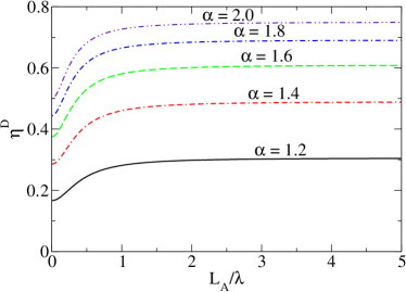
Figure 3: (Color online)Efficiency of the Isoenergetic Cycle, calculated after Eq.(LABEL:eq28), as a function of the expansion parameter $\alpha=L_{C}/L_{B}$.

According to the previous analysis, the heat exchanged by the system with the environment along the iso-energetic process is given by

$$Q_{1\rightarrow 2}=\sum_{n=1}^{\infty}\int_{L_{1}}^{L_{2}}E_{n}(L)\frac{dp_{n}(L)}{dL}\,dL.$$ (31)

Evidently, Eq.(28) combined with the normalization condition Eq.(22) are not enough to uniquely define the coefficients $p_{n}(L)$ along the iso-energetic trajectory. An exception is the case when the energy scale of all the processes involved is such that only transitions between the ground state ($n=1$) and the first excited state ($n=2$) are possible. In this effective two-level spectrum, combining Eq.(28) with the normalization condition Eq.(22), the trajectory for the iso-energetic process is described by the following relation

$$p_{1}(L) = \frac{E_{2}(L_{1})-E_{2}(L)}{E_{1}(L)-E_{2}(L)}+\frac{E_{1}(L_{1})-E_{2}(L_{1})}{E_{1}(L)-E_{2}(L)}p_{1}(L_{1}),$$

with $p_{2}(L)=1-p_{1}(L)$ after the normalization condition Eq.(22). The heat exchanged by the system with the environment during an iso-enegetic trajectory connecting the initial and final states $L_{1}\rightarrow L_{2}$, for the case of a Dirac particle, is given by the expression

$$-Q_{1\rightarrow 2}=\left[E_{2}^{D}(L_{1})+\left(E_{1}^{D}(L_{1})-E_{2}^{D}(L_{1})\right)\right.$$

$$\left.\times p_{1}(L_{1})\right]\ln\left[\frac{E_{1}^{D}(L_{2})-E_{2}^{D}(L_{2})}{E_{1}^{D}(L_{1})-E_{2}^{D}(L_{1})}\right]+2(mc^{2})\ln\left(\frac{L_{2}}{L_{1}}\right)$$

$$+(mc^{2})\ln\left[\frac{mc^{2}+E_{2}^{D}(L_{2})}{mc^{2}+E_{2}^{D}(L_{1})}\frac{mc^{2}+E_{1}^{D}(L_{2})}{mc^{2}+E_{1}^{D}(L_{1})}\right]$$ (33)

where $E_{n}^{D}(L)$ was defined in Eq.(18).

For the effective two-level system previously described, we shall conceive a cycle, as depicted in Figure 1, which starts in the ground state with $p_{1}(L_{A})=1$. Then, the system experiences an iso-energetic expansion from $L_{A}\rightarrow L_{B}>L_{A}$. Then, it experiences an iso-entropic expansion from $L_{B}\rightarrow L_{C}>L_{B}$, then an iso-energetic compression $L_{C}\rightarrow L_{D}<L_{C}$, and finally it goes back to the initial ground state through an iso-entropic compression $L_{D}\rightarrow L_{A}$.

We shall assume that the final state after the iso-energetic process $L_{A}\rightarrow L_{B}$ corresponds to maximal expansion, that is, the system ends completely localized in the excited state $n=2$. In this condition, Eq.(LABEL:eq19) reduces to

$$p_{1}(L_{B})=0,\,\,\,\,p_{2}(L_{B})=1.$$ (34)

The condition of total energy conservation between the initial and final states connected through an iso-energetic process, for maximal expansion, leads to the equation

$$p_{1}(L_{A})E_{1}(L_{A})=p_{2}(L_{B})E_{2}(L_{B}),$$ (35)

where $p_{1}(L_{A})=p_{2}(L_{B})=1$ for maximal expansion. Therefore Eq.(35), given the Dirac spectrum Eq.(18), implies that $L_{B}/L_{A}=2$.

The heat released to the environment along this first stage of the cycle is calculated after Eq.(33),

$$-Q_{A\rightarrow B} = E_{1}^{D}(L_{A})\ln\left[\frac{E_{2}^{D}(L_{A})-E_{1}^{D}(L_{A})}{E_{2}^{D}(2L_{A})-E_{1}^{D}(2L_{A})}\right]$$ (36)

$$+ mc^{2}\ln\left[\frac{1}{4}\left\{\frac{mc^{2}+E_{2}^{D}(L_{A})}{mc^{2}+E_{1}^{D}(2L_{A})}\right\}\right].$$

The next process is an iso-entropic expansion, characterized by the condition $p_{2}(L_{B})=p_{2}(L_{C})=1$. We shall define the expansion parameter $\alpha\equiv L_{C}/L_{B}>1$. The work performed during this stage, with $L_{B}=2L_{A}$ (as discussed before), is calculated from Eq.(27),

$$W_{B\rightarrow C} = mc^{2}\left[\sqrt{1+\left(\frac{\lambda}{2L_{A}}\right)^{2}}-\sqrt{1+\left(\frac{\lambda}{2\alpha L_{A}}\right)^{2}}\right].$$

The cycle continues with a maximal compression process from $L_{C}=2\alpha L_{A}$ to $L_{D}=\alpha L_{A}$ under iso-energetic conditions. The energy conservation condition is in this case similar to Eq.(35), with $p_{2}(L_{C})=p_{1}(L_{D})=1$. The heat exchanged by the system with the environment along this process, applying Eq.(33), is given by the expression

$$-Q_{C\rightarrow D} = E_{2}^{D}(2\alpha L_{A})\ln\left[\frac{E_{2}^{D}(\alpha L_{A})-E_{1}^{D}(\alpha L_{A})}{E_{2}^{D}(2\alpha L_{A})-E_{1}^{D}(2\alpha L_{A})}\right]$$ (38)

$$+mc^{2}\ln\left[\frac{1}{4}\left\{\frac{mc^{2}+E_{2}^{D}(\alpha L_{A})}{mc^{2}+E_{1}^{D}(2\alpha L_{A})}\right\}\right]$$

where $E_{n}^{D}(L)$ was defined in Eq.(18). The last path along the cycle is an adiabatic process, which returns the system to its initial ground state with $p_{1}(L_{D})=p_{1}(L_{A})=1$. The work performed during this final stage, as obtained by applying Eq.(27), is given by

$$W_{D\rightarrow A} = mc^{2}\left[\sqrt{1+\left(\frac{\lambda}{2\alpha L_{A}}\right)^{2}}-\sqrt{1+\left(\frac{\lambda}{2L_{A}}\right)^{2}}\right].$$

It is interesting to check that the work along the two iso-entropic trajectories cancels, that is $W_{B\rightarrow C}+W_{D\rightarrow A}=0$. Therefore, the efficiency of the cycle is defined by the ratio

$$\eta^{D}=1-\frac{Q_{C\rightarrow D}}{Q_{A\rightarrow B}}.$$ (40)

When substituting the corresponding expressions from Eq.(36) and Eq.(38) into Eq.(40), we obtain the explicit analytical expression

$$\eta^{D} = 1-\frac{\ln\left[\frac{1}{4}\frac{1+\theta(\alpha L_{A}/2)}{1+\theta(2\alpha L_{A})}\left\{\frac{\theta(\alpha L_{A}/2)-\theta(\alpha L_{A})}{\theta(\alpha L_{A})-\theta(2\alpha L_{A})}\right\}^{\theta(\alpha L_{A})}\right]}{\ln\left[\frac{1}{4}\frac{1+\theta(L_{A}/2)}{1+\theta(2L_{A})}\left\{\frac{\theta(L_{A}/2)-\theta(L_{A})}{\theta(L_{A})-\theta(2L_{A})}\right\}^{\theta(L_{A})}\right]}.$$

Here, we have defined the function $\theta(L)=\sqrt{1+(\lambda/2L)^{2}}$, with $\lambda=2\pi\hbar/(mc)$ the Compton wavelength. It is important to remark that in the non-relativistic limit $\lambda/L\rightarrow 0$, the expression in Eq.(40) reduces to the known Schrödinger limit

$$\lim_{\lambda/L\rightarrow 0}\eta^{D}=1-1/\alpha^{2}.$$ (42)

In the ”ultra-relativistic” case of a massless Dirac particle, $\lambda/L\rightarrow\infty$, the efficiency converges to the length independent limit

$$\lim_{\lambda/L\rightarrow\infty}\eta^{D}=1-1/\alpha.$$ (43)

The trend of the efficiency is shown in between both limits in Figure 3. It is worth to remark that, since the expansion parameter $\alpha=L_{C}/L_{B}>1$, the efficiency in the strict non-relativistic (Schrödinger) regime $\lambda/L\rightarrow 0$ Eq.(42) is the highest possible one. This is also clear from the asymptotics of the curves displayed in Fig. 3, where the ”ultra-relativistic” limit corresponding to massless Dirac particles ($\lambda/L\rightarrow\infty$) indeed represents the less efficient regime for a fixed expansion parameter $\alpha$.

V The Quantum Carnot cycle

In this section, we shall discuss the quantum version of the Carnot cycle, as applied to the statistical ensemble of Dirac single-particle systems under consideration. The thermodynamic cycle which defines the corresponding heat engine is composed of four stages or trajectories in Hilbert’s space: Two isothermal and two iso-entropic processes.

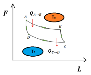
Figure 4: (Color online)Pictorial description of the Force versus width of the potential well, for the Quantum Carnot Cycle described in the text.

In the first stage, the system is brought into contact with a thermal reservoir at temperature $T_{H}$. By keeping isothermal conditions, the width of the potential well is expanded from $L_{A}\rightarrow L_{B}$. Since thermal equilibrium with the reservoir is assumed along this process, the von Neumann entropy of the system achieves a maximum for the Boltzmann distribution von Neumann (1955); Tolman (1938)

$$p_{n}(L,\beta_{H})=\left[Z(L,\beta_{H})\right]^{-1}e^{-\beta_{H}E_{n}^{D}(L)},$$ (44)

with $\beta=(k_{B}T)^{-1}$, and the normalization factor is given by the partition function

$$Z(L,\beta)=\sum_{n=0}^{\infty}e^{-\beta E_{n}^{D}(L)}\sim\frac{2L}{\lambda}e^{\beta mc^{2}}K_{1}(\beta mc^{2}).$$ (45)

Here, the second expression, as shown in Appendix, is the continuum approximation to the discrete sum, valid in the physically relevant regime $\lambda\ll L$. Here, $K_{1}(x)$ is a modified Bessel function of the second kind.

From a similar analysis as in the previous section, we conclude that the heat exchanged by the system to the thermal reservoir is given by

$$Q_{A\rightarrow B} = \int_{L_{A}}^{L_{B}}\sum_{n=0}^{\infty}E_{n}(L)\frac{dp_{n}(L,\beta_{H})}{dL}dL$$ (46)

$$= -\frac{\partial\ln\left(\frac{Z(L_{B},\beta_{H})}{Z(L_{A},\beta_{H})}\right)}{\partial\beta_{H}}+\beta_{H}^{-1}\ln\left(\frac{Z(L_{B},\beta_{H})}{Z(L_{A},\beta_{H})}\right)$$

$$= \beta_{H}^{-1}\ln\left(\frac{L_{B}}{L_{A}}\right).$$

In the second line, we have done integration by parts, and we made direct use of the definition Eq.(43) of the partition function. The final result follows from substituting the explicit expression for the partition function Eq.(45).

Similarly, during the third stage of the cycle, the system is again brought into contact with a thermal reservoir, but at a lower temperature $T_{C}<T_{H}$. Therefore, the probability distribution of states in the ensemble is $p_{n}(L,\beta_{C})$, as defined in Eq.(44), but with $T_{C}$ instead of $T_{H}$. The heat released to the reservoir during this stage is given by the expression

$$Q_{C\rightarrow D}=\beta_{C}^{-1}\ln\left(\frac{L_{D}}{L_{C}}\right).$$ (47)

The second and fourth stages of the cycle constitute iso-entropic trajectories. In order to analyze these stages, we shall derive the ”equation of state” for the statistical ensemble of single-particle systems. When substituting the Boltzmann distribution $p_{n}(\beta,L)=\left[Z(\beta,L)\right]^{-1}\exp(-\beta E_{n}^{D}(L))$ into the expression for the von Neumann entropy Eq.(23), we obtain the relation

$$S=T^{-1}E+k_{B}\ln Z(\beta,L).$$ (48)

Here, $E=\langle\hat{H}\rangle$ is the ensemble-average energy, as defined by Eq.(24). The equation of state is obtained from Eq.(48) as

$$F = -\left(\frac{\partial E}{\partial L}\right)_{S}=k_{B}T\frac{\partial}{\partial L}\ln Z(\beta,L)$$ (49)

$$= \frac{k_{B}T}{L}.$$

In the last line, we have used the explicit analytical expression Eq.(45) for the partition function to calculate the derivative. The equation of state Eq.(49) reflects that the ensemble of systems behaves as a one-dimensional ideal gas. This is not surprising, since the ensemble-average energy is given by

$$E = \langle\hat{H}\rangle=-\frac{\partial}{\partial\beta}\ln Z(\beta,L)$$ (50)

$$= mc^{2}\left(-1-\frac{d}{dz}\ln K_{1}(z)\right),$$

where we have substituted explicitly the expression for the partition function, and in the final step we defined $z=\beta\,mc^{2}$. Here, $K_{1}(x)$ is a modified Bessel function of the second kind. Eq.(50) shows that the ensemble average energy of the system is a function of the temperature solely, from which the ideal gas equation of state follows as a natural consequence. We can thus define the ”specific heat” at constant length, which after Eq.(50) is given by

$$C_{L} = \left(\frac{\partial E}{\partial T}\right)_{L}=\frac{dE}{dT}=k_{B}z^{2}\frac{d^{2}}{dz^{2}}\ln K_{1}(z),$$ (51)

where $z=\beta mc^{2}$. It is interesting to remark that, based on the asymptotic behavior of the modified Bessel functions of the second kind $K_{n}(z)\sim\sqrt{\pi/2}z^{-1/2}\exp(-z)+O(z^{-1})$, the specific heat defined in Eq.(51) presents the asymptotic limit $C_{L}\rightarrow k_{B}/2$ when $k_{B}T\ll mc^{2}$. This is the well known result for a classic non-relativistic ideal gas in one dimension. This feature and the general temperature dependence of the ensemble specific heat is displayed in Fig. 6. The change in the ensemble averaged energy of the system, for a general process, is $dE=TdS-FdL$. Since the ensemble-average energy is a function of temperature only, the differential equation for an iso-entropic trajectory ($dS=0$) isnot (b)

$$dE=C_{L}dT=-FdL=-k_{B}T\frac{dL}{L}.$$ (52)

Separating variables, after some algebra we obtain

$$z\frac{d^{2}}{dz^{2}}\ln K_{1}(z)=\frac{dL}{L}.$$ (53)

Integrating Eq.(53) between initial conditions $(z_{0},L_{0})$ and final conditions $(z,L)$, we have

$$\frac{L}{L_{0}}=\frac{K_{1}(z_{0})}{K_{1}(z)}e^{-z\frac{K_{0}(z)}{K_{1}(z)}+z_{0}\frac{K_{0}(z_{0})}{K_{1}(z_{0})}}.$$ (54)

Here, we made use of the identity for the modified Bessel function of the second kind $K_{1}^{{}^{\prime}}(z)=-K_{0}(z)-z^{-1}K_{1}(z)$, with $z=\beta mc^{2}$. It is interesting to check that in the non-relativistic limit $z\gg 1$, given the asymptotic behavior of the modified Bessel function of the second kind $K_{n}(z)\sim\sqrt{\pi/2}z^{-1/2}\exp(-z)+O(z^{-1})$, Eq.(54) reduces to $LT^{1/2}=cnt.$ for the iso-entropic trajectory. On the other hand, in the ”ultra-relativistic” limit of a massless Dirac particle with $z\rightarrow 0$, the iso-entropic trajectory is given by the equation $LT=cnt.$

We are now in conditions to discuss the second and fourth stages of the Carnot cycle. The second stage of the process corresponds to an iso-entropic trajectory, parameterized in differential and integral form by Eqs.(53) and (54), respectively. The work performed by the system during this process is given by

$$W_{B\rightarrow C} = -\int_{L_{B}}^{L_{C}}FdL=-\int_{L_{B}}^{L_{C}}k_{B}T\frac{dL}{L}$$ (55)

$$= -mc^{2}\int_{z_{H}}^{z_{C}}\frac{d^{2}}{dz^{2}}\ln K_{1}(z)dz$$

Here, in the second line we have used the differential equation defining the iso-entropic trajectory, Eq.(53). Evaluating the integral in Eq.(55), we explicitly obtain

$$W_{B\rightarrow C}=k_{B}(T_{C}-T_{H})-mc^{2}\left[\frac{K_{0}(z_{C})}{K_{1}(z_{C})}-\frac{K_{0}(z_{H})}{K_{1}(z_{H})}\right]$$ (56)

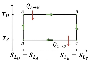
Figure 5: (Color online)Pictorial description of the Force versus width of the potential well for the Quantum Carnot Cycle.

The fourth and final stage of the cycle also corresponds to an iso-entropic trajectory $L_{D}\rightarrow L_{A}$, and the work performed by the system against the external applied force is obtained similarly as in Eq.(55),

$$W_{D\rightarrow A} = -\int_{L_{D}}^{L_{A}}FdL$$

$$= k_{B}(T_{H}-T_{C})-mc^{2}\left[\frac{K_{0}(z_{H})}{K_{1}(z_{H})}-\frac{K_{0}(z_{C})}{K_{1}(z_{C})}\right].$$

Clearly, after Eqs.(56) and (V), we have $W_{B\rightarrow C}+W_{D\rightarrow A}=0$, and hence the contribution of the work along the iso-entropic trajectories vanishes.

From the equation for the iso-entropic trajectory Eq.(54), we conclude that the length ratios are determined by the temperatures of the thermal reservoirs,

$$\frac{L_{C}}{L_{B}}=\frac{L_{D}}{L_{A}}=\frac{K_{1}(z_{H})}{K_{1}(z_{C})}e^{-z_{C}\frac{K_{0}(z_{C})}{K_{1}(z_{C})}+z_{H}\frac{K_{0}(z_{H})}{K_{1}(z_{H})}}.$$ (58)

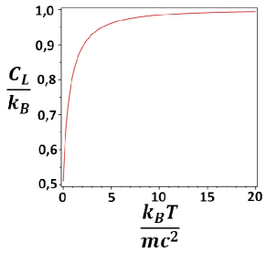
Figure 6: (Color online)Specific heat of the statistical ensemble of single Dirac-particle systems, after Eq.(51), as a function of temperature.

From Eq.(58), we also obtain $L_{A}/L_{B}=L_{D}/L_{C}$. Substituting this relation in the expression for the efficiency of the cycle, from Eq.(46) and Eq.(47) we have

$$\eta^{C} = 1-\frac{Q_{C\rightarrow D}}{Q_{A\rightarrow B}}=1-\frac{T_{C}}{T_{H}}\frac{\ln(L_{D}/L_{C})}{\ln(L_{B}/L_{A})}$$ (59)

$$= 1-\frac{T_{C}}{T_{H}}.$$

Therefore, we have recovered the expression for the efficiency identical to the classical Carnot cycle.

VI Conclusions

By considering as a ”working substance” the statistical ensemble for a Dirac single-particle system trapped in a one-dimensional potential well, we have analyzed two different schemes for a quantum heat engine. The first, that we have referred to as the Isoenergetic cycle, consists of two iso-entropic and two isoenergetic trajectories. We obtained an explicit expression for the efficiency of this cycle and showed that our analytical result, in the non-relativistic limit $\lambda/L\rightarrow 0$, reduces to the corresponding one for a Schrödinger particle, as reported in the literature Bender et al. (2002). Our results also indicate that the efficiency for the Isoenergetic cycle is higher in the non-relativistic region of parameters, that is for $L\gg\lambda$, when comparing at the same compressibility ratios $\alpha=L_{C}/L_{B}>1$. An exception is the case of massless Dirac particles, with $\lambda=\infty$, where it is not possible to achieve non-relativistic conditions. This is of potential practical interest for graphene systems, where conduction electrons are indeed described as massless chiral Dirac fermionsPeres (2010); Castro et al. (2009); Muñoz et al. (2010); Muñoz (2012).

As a second candidate for a quantum heat engine, we discussed a version of the Carnot cycle, composed by two iso-thermal and two iso-entropic trajectories. In order to achieve iso-thermal conditions, we consider that the single-particle system is in thermal equilibrium with macroscopic reservoirs at temperatures $T_{C}<T_{H}$, respectively. Therefore, the statistical ensemble under consideration is described by the density matrix $\hat{\rho}=e^{-\beta\hat{H}}/Z$, with $Z[\beta,L]={\rm{Tr}}e^{-\beta\hat{H}}$ the partition function. We showed that the statistical properties of the ensemble are such that an equation of state can be defined, as well as a specific heat, in analogy with a classical ideal gas in one dimension. We obtained the equation for the iso-entropic trajectory, which in the non-relativistic limit $k_{B}T\ll mc^{2}$ reduces to the classical result $LT^{1/2}=cnt$. On the other hand, we also showed that in the ”ultra-relativistic” limit of a massless Dirac particle, as for instance conduction electrons in graphene, the iso-entropic trajectory is defined by the equation $LT=cnt.$ We also showed that the efficiency for the Quantum Carnot cycle satisfies the same relation that the classical one in terms of the temperatures of the thermostats, that is $\eta=1-T_{C}/T_{H}$. Therefore, thermodynamics is remarkably robust: The Carnot limit holds classically just as it does in the quantum regime, even in the quantum-relativistic limit.

Finally, we conclude by saying that the general statistical mechanical analysis presented in this work, can in principle be applied to predict the thermodynamics of other one-dimensional single-particle systems of potential interest, with different energy spectra.

Appendix A

We shall consider the physically meaningful eigenfunctions of the self-adjoint extension Thaller (1956); Carreau et al. (1990); Alonso et al. (1997); Alberto et al. (1996) of the free Dirac Hamiltonian

$$\hat{H}_{0}=-i\hbar c\,\bm{\alpha}\cdot\nabla+mc^{2}\hat{\beta},$$ (60)

whose domain $\mathcal{D}(\hat{H}_{0})\subset\mathcal{H}_{\Omega}$ is a dense proper subset of the Hilbert space $\mathcal{H}_{\Omega}=L^{2}(\Omega)\oplus L^{2}(\Omega)\oplus L^{2}(\Omega)\oplus L^{2}(\Omega)\equiv L^{2}(\Omega,\mathbb{C}^{4})$ of square-integrable (complex-valued) 4-component spinors in the closed interval $x\in\Omega=[-L/2,L/2]$. It is convenient to describe the four-component spinor $\hat{\psi}(x)=(\phi_{1},\phi_{2},\chi_{1},\chi_{2})$ as composed by a pair of two-component spinors $\phi(x)=(\phi_{1},\phi_{2})$ and $\chi(x)=(\chi_{1},\chi_{2})$. In this notation, $\phi(x)$ is denoted as the ”large” component, while $\chi(x)$ is referred as the ”small” component.

In general, the domain of $\hat{H}_{0}$ and its adjoint $\hat{H}_{0}^{\dagger}$ verify $\mathcal{D}(\hat{H}_{0})\subseteq\mathcal{D}(\hat{H}_{0}^{\dagger})$ Thaller (1956). On the other hand, physics requires for $\hat{H}_{0}$ to be self adjoint. This condition is mathematically obtained by looking for a self-adjoint extension of $\hat{H}_{0}$, upon imposing appropriate boundary conditions for the spinors at the boundary $\partial\Omega$ of the finite region $\Omega$. Therefore, for any pair of spinors in the domain of the self-adjoint extension of the free Hamiltonian, we request for their inner product to satisfy

$$\left(\hat{\psi}_{a},\hat{H}\hat{\psi}_{b}\right) - \left(\hat{H}\hat{\psi}_{a},\hat{\psi}_{b}\right)$$ (61)

$$\equiv \int_{\Omega}\left[\hat{\psi}_{a}^{\dagger}\hat{H}\hat{\psi}_{b}-\left(\hat{H}\hat{\psi}_{a}\right)^{\dagger}\hat{\psi}_{b}\right]dV$$

$$= -i\hbar c\int_{\partial\Omega}\hat{\mathbf{n}}\cdot\hat{\psi}_{a}^{\dagger}{\bm{\alpha}}\hat{\psi}_{b}dS=0.$$

Here, $\hat{\mathbf{n}}$ is a unit vector normal to the surface $\partial\Omega$. We have used integration by parts, and applied the generalized divergence theorem to transform the volume integral over the region $\Omega$ into an integral over the boundary $\partial\Omega$. Notice that, in particular, condition Eq.(61) implies that for all $\hat{\psi}(x)\in\mathcal{D}(\hat{H}_{0})$,

$$\left.\hat{\mathbf{n}}\cdot\hat{\psi}^{\dagger}c{\bm{\alpha}}\hat{\psi}\right|_{\partial\Omega}\equiv\left.\hat{\mathbf{n}}\cdot{\mathbf{j}}\right|_{\partial\Omega}=0.$$ (62)

This mathematical condition has a rather obvious physical interpretation, since the probability current vanishing at the boundary $\partial\Omega$ implies that the particle is indeed ”trapped” inside the finite region $\Omega$. We remark that this mathematical approach, with analogous boundary condition, has been used in the past to model confinement of hadrons in a finite region of space (so-called ”bag model”) Chodos et al. (1974a, b).

Therefore, the eigenvalue problem for the self-adjoint extension of the free Dirac Hamiltonian in the one-dimensional region $\Omega=[-L/2,L/2]$,

$$\hat{H}_{0}\hat{\psi}=E\hat{\psi}$$ (63)

must be subject to the boundary conditions

$$j^{1}(x=\pm L/2)=0.$$ (64)

It is convenient to write Eq.(63) as a pair of coupled differential equations for each of the two components of the spinor,

$$-i\hbar c\,\bm{\sigma}\cdot\nabla\chi+mc^{2}\phi = E\phi$$

$$-i\hbar c\,\bm{\sigma}\cdot\nabla\phi-mc^{2}\chi = E\chi.$$ (65)

From Eq.(65), we obtain

$$\chi=\frac{-i\hbar c}{E+mc^{2}}\bm{\sigma}\cdot\nabla\phi.$$ (66)

This equation determines the ”small” component $\chi$ of the spinor in terms of the ”large” component $\phi$. The last is obtained upon substitution of Eq.(66) into Eq.(65), as the solution to the eigenvalue problem

$$\bm{\sigma}\cdot\nabla\left(\bm{\sigma}\cdot\nabla\phi\right)=-\frac{E^{2}-m^{2}c^{4}}{\hbar^{2}c^{2}}\phi.$$ (67)

For the one-dimensional region we are concerned $\Omega=[-L/2,L/2]$, we have $\phi=\phi(x)$, and Eq.(67) becomes

$$\frac{d^{2}}{dx^{2}}\left(\begin{array}[]{c}\phi_{1}\\ \phi_{2}\end{array}\right)+k^{2}\left(\begin{array}[]{c}\phi_{1}\\ \phi_{2}\end{array}\right)=0.$$ (72)

Here, we defined the wavenumber

$$k^{2}\equiv(E^{2}-m^{2}c^{4})/(\hbar^{2}c^{2}).$$ (73)

The general solution to Eq.(72) is

$$\phi(x) = A_{1}\left(\begin{array}[]{c}1\\ 0\end{array}\right)e^{ikx}+A_{2}\left(\begin{array}[]{c}0\\ 1\end{array}\right)e^{ikx}$$ (78)

$$+ B_{1}\left(\begin{array}[]{c}1\\ 0\end{array}\right)e^{-ikx}+B_{2}\left(\begin{array}[]{c}0\\ 1\end{array}\right)e^{-ikx}.$$ (83)

We shall consider a spin-polarized particle, so we select the spin up solutions by setting $A_{2}=0$, $B_{2}=0$. With this choice, from Eq.(66) we obtain $\chi$, which combined with Eq.(83) gives the general solution for the four-component spinor

$$\hat{\psi}(x)=A_{1}\left(\begin{array}[]{c}1\\ 0\\ 0\\ \frac{\hbar ck}{E+mc^{2}}\end{array}\right)e^{ikx}+B_{1}\left(\begin{array}[]{c}1\\ 0\\ 0\\ \frac{-\hbar ck}{E+mc^{2}}\end{array}\right)e^{-ikx}.$$ (92)

By requesting for the condition of vanishing current at the boundaries Eq.(64), we obtain

$$j^{1}(x) = \hat{\psi}^{\dagger}(x)c\hat{\alpha}_{1}\hat{\psi}(x)$$ (93)

$$= \frac{2\hbar c^{2}k}{E+mc^{2}}\left(|A_{1}|^{2}-|B_{1}|^{2}\right)=0,$$

which implies $|A_{1}|=|B_{1}|$. We express this condition in the form

$$B_{1}=A_{1}e^{i\theta},$$ (94)

with $\theta$ the relative phase between the two (complex) amplitudes. Therefore, we obtain an entire family of (spin polarized) eigenfunctions for the self-adjoint extension of the Dirac operator

$$\hat{\psi}(x)=A_{1}\left(\begin{array}[]{c}e^{ikx}+e^{-ikx+i\theta}\\ 0\\ 0\\ \frac{\hbar ck}{E+mc^{2}}\left[e^{ikx}-e^{-ikx+i\theta}\right]\end{array}\right)$$ (99)

Among all the possible phases $\theta$ in Eq.(99), the appropriate physical solution should converge to the solution of the equivalent Schrödinger problem in the non-relativistic limit $\hbar k\ll mc$. In this former case, the Schrödinger (S) wave functions are of the form $\varphi_{n}^{S}(x)=A\sin(n\pi(x-L/2)/L)$, with corresponding probability density $\rho^{S}(x)\propto\sin^{2}(n\pi(x-L/2)/L)$. Therefore, we set the phase difference $\theta=kL+\pi$,

$$\hat{\psi}(x)=A\left(\begin{array}[]{c}\sin(k(x-L/2))\\ 0\\ 0\\ -\frac{i\hbar ck}{E+mc^{2}}\cos(k(x-L/2))\end{array}\right).$$ (104)

where we have defined $A\equiv 2iA_{1}e^{ikL/2}$. Clearly, the ”small” component of the spinor in Eq.(104) vanishes in the non-relativistic limit $\hbar k\ll mc$, thus leading to a probability density $\rho(x)=\hat{\psi}^{\dagger}(x)\hat{\psi}(x)\propto\sin^{2}(k(x-L/2))$, in agreement with the Schrödinger result.

Eq.(104) satisfies the condition $j^{1}(x)=j^{1}(\pm L/2)=0$, where the probability current is continuous and vanishes everywhere, in particular at the boundaries of the confining region.

A fundamental discrete symmetry of the Dirac Hamiltonian is its invariance under parity Sakurai (1967); Bjorken and Drell (1964); Thaller (1956) ($\hat{P}$: $x\rightarrow-x$, $p_{x}\rightarrow-p_{x}$), $[\hat{H}_{0},\hat{P}]=0$, which corresponds to a mirror spatial reflection, by leaving the spin direction invariant. It is straightforward to show that under parity, the spinor transforms as Bjorken and Drell (1964); Sakurai (1967); Thaller (1956) $\hat{P}\hat{\psi}(x)\hat{P}^{-1}=e^{i\phi}\hat{\beta}\hat{\psi}(-x)$. On the other hand, the probability density defined as $\rho(x)=\hat{\psi}^{\dagger}(x)\hat{\psi}(x)=c^{-1}j^{0}(x)$ is the time-component of the Lorentz 4-vector $j^{\mu}=c\bar{\psi}(x)\gamma^{\mu}\hat{\psi}(x)$, with $\bar{\psi}(x)\equiv\gamma^{0}\hat{\psi}^{\dagger}(x)$, and where the explicit covariant notation $\gamma^{i}=\hat{\beta}\hat{\alpha}_{i}$ (i=1,2,3), $\gamma^{0}=\hat{\beta}$ was invoked. Under parity, the space components of a Lorentz 4-vector change sign, whereas the time component remains invariant Bjorken and Drell (1964); Sakurai (1967); Thaller (1956), and hence $\rho(-x)=\rho(x)$. Therefore, we demand for the eigenfunctions of the self-adjoint extension of the Dirac Hamiltonian to possess this inversion symmetry,

$$\rho(x)=\rho(-x), \forall x\in[-L/2,L/2].$$ (105)

From Eq.(104), and the definition of the probability density

$$\rho(\pm x) = \hat{\psi}^{\dagger}(\pm x)\hat{\psi}(\pm x)$$ (106)

$$= 4|A_{1}|^{2}\left[1-\left(1-\frac{\hbar^{2}c^{2}k^{2}}{(E+mc^{2})^{2}}\right)\right.$$

$$\left.\times\cos^{2}(k(\pm x-L/2))\right]$$

By using the trigonometric identity $\cos^{2}(\alpha)=(1+\cos(2\alpha))/2$, we obtain that the condition for Eq.(105) to be satisfied is

$$\cos(kL+2kx)=\cos(kL-2kx), \forall x\in[-L/2,L/2]$$ (107)

This is further simplified to yield the equation

$$2\sin(2kx)\sin(kL)=0, \forall x\in[-L/2,L/2],$$ (108)

whose solutions are

$$k\equiv k_{n}=\frac{n\pi}{L}, n\in\mathbb{N}.$$ (109)

Therefore, the spectrum of the self-adjoint extension of the Dirac Hamiltonian representing a single particle trapped in the one-dimensional infinite potential well is discrete, and given by

$$E_{n}=\sqrt{c^{2}\hbar^{2}k_{n}^{2}+m^{2}c^{4}}=\sqrt{\left(\frac{\hbar cn\pi}{L}\right)^{2}+m^{2}c^{4}}.$$ (110)

By introducing the definition of the Compton wavelength $\lambda=2\pi\hbar/(mc)$, the spinor-eigenfunction Eq.(104), with $k_{n}$ quantized by Eq.(109), can be written as Eq.(17) in the main text. By subtracting the rest energy from Eq.(110), one obtains Eq.(18) for the Dirac particle spectrum.

Appendix B

We here discuss the continuum approximation to the discrete partition function Eq.(43).

$$Z(L,\beta)=\sum_{n=0}^{\infty}e^{-\beta mc^{2}\left(\sqrt{1+\left(\frac{n\lambda}{2L}\right)^{2}}-1\right)}$$

Here, let us define the discrete variable $x_{n}=n\lambda/(2L)$. The spacing between two consecutive values is given by $\Delta x=x_{n+1}-x_{n}=\lambda/(2L)$, and hence the expression for the partition function can be written as

$$Z(L,\beta)=\frac{2L}{\lambda}\sum_{n=0}^{\infty}\Delta x\,e^{-\beta mc^{2}\left(\sqrt{1+x_{n}^{2}}-1\right)}$$

For physically relevant sizes of the potential well, we shall have $\lambda/L\ll 1$, which allow us to take the continuum limit in the sense of a Riemann sum for the previous equation,

$$Z(L,\beta) \rightarrow\frac{2L}{\lambda}\int_{0}^{\infty}dxe^{-\beta mc^{2}\left(\sqrt{1+x^{2}}-1\right)}$$

$$= \frac{2L}{\lambda}\int_{0}^{\infty}dte^{-\beta mc^{2}\left(\cosh(t)-1\right)}\cosh(t)$$

$$= \frac{2L}{\lambda}e^{\beta mc^{2}}K_{1}\left(\beta mc^{2}\right).$$

Here, in the second line we have made the substitution $x=\sinh(t)$, and $K_{1}(x)$ is a modified Bessel function of the second kind.

References

- Fermi (1936) E. Fermi, Thermodynamics (Dover, 1936).
- Callen (1985) H. B. Callen, Thermodynamics and an Introduction to Thermostatistics (John Wiley and Sons, 1985), 2nd ed.
- Bender et al. (2002) C. M. Bender, D. C. Brody, and B. K. Meister, Proc. R. Soc. Lond. A 458, 1519 (2002).
- Bender et al. (2000) C. M. Bender, D. C. Brody, and B. K. Meister, arXiv:quant-ph/0007002v1 (2000).
- Wang et al. (2011) J. Wang, J. He, and X. He, Phys. Rev. E 84, 041127 (2011).
- Wang and He (2012) J. Wang and J. He, J. Appl. Phys. 111, 043505 (2012).
- Quan et al. (2006) H. T. Quan, P. Zhang, and C. P. Sun, Phys. Rev. E 73, 036122 (2006).
- Arnaud et al. (2002) J. Arnaud, L. Chusseau, and F. Philippe, Eur. J. Phys. 23, 489 (2002).
- Latifah and Purwanto (2011) E. Latifah and A. Purwanto, J. Mod. Phys. 2, 1366 (2011).
- Quan et al. (2007) T. H. Quan, Y. xi Liu, C. P. Sun, and F. Nori, Phys. Rev. E 76, 031105 (2007).
- Quan et al. (2005) H. T. Quan, P. Zhang, and C. P. Sun, arXiv:quant-ph/0504118v3 (2005).
- Peres (2010) N. M. R. Peres, Rev. Mod. Phys. 82, 2673 (2010).
- Castro et al. (2009) A. H. Castro, F. Guinea, N. M. R. Peres, K. S. Novoselov, and A. K. Geim, Rev. Mod. Phys. 81, 109 (2009).
- Muñoz et al. (2010) E. Muñoz, J. Lu, and B. I. Yakobson, Nano Lett. 10, 1652 (2010).
- Muñoz (2012) E. Muñoz, J. Phys.: Condens. Matter 24, 195302 (2012).
- Thaller (1956) B. Thaller, The Dirac Equation (Springer-Verlag, 1956).
- Bjorken and Drell (1964) J. D. Bjorken and S. D. Drell, Relativistic Quantum Mechanics (Mc Graw-Hill, 1964).
- Sakurai (1967) J. J. Sakurai, Advanced Quantum Mechanics (Addison-Wesley, 1967).
- Carreau et al. (1990) M. Carreau, E. Farhi, and S. Gutmann, Phys. Rev. D 42, 1194 (1990).
- Alonso et al. (1997) V. Alonso, S. D. Vincenzo, and L. Mondino, Eur. J. Phys. 18, 315 (1997).
- Alberto et al. (1996) P. Alberto, C. Fiolhais, and V. M. S. Gil, Eur. J. Phys. 17, 19 (1996).
- Chodos et al. (1974a) A. Chodos, R. L. Jaffe, C. B. Thorn, and W. F. Weisskopf, Phys. Rev. D 9, 3471 (1974a).
- Chodos et al. (1974b) A. Chodos, R. L. Jaffe, and C. B. Thorn, Phys. Rev. D 8, 2599 (1974b).
- von Neumann (1955) J. von Neumann, Mathematical Foundations of Quantum Mechanics (Princeton University Press, 1955).
- Tolman (1938) R. C. Tolman, The Principles of Statistical Mechanics (Oxford, 1938).
- not (a) A necessary condition for entropy to remain constant is . This is clearly less stringent than the sufficient condition for all n.
- not (b) The necessary condition for an iso-entropic trajectory in this case differs from the more stringent sufficient condition requested in the E-Carnot cycle (see note 18). In terms of the distribution , a trajectory with is defined by . This implies that must change as a function of along the process in order to satisfy the iso-entropic constraint.