Constraints on the primordial gravitational waves with variable sound speed from current CMB data
Abstract:
We make a comprehensive investigation of the observational effect of the inflation consistency relation. We focus on the general single-field inflation model with the consistency relation , and investigate the observational constraints of sound speed by using the Seven-Year WMAP data, the BICEP tensor power spectrum data, and the constraints on and from the Five-Year WMAP observations. We find that the constraints on the tensor-to-scalar ratio is much tighter if is small, since a large tilt is strongly constrained by the observations. We obtain and () for =, and models at confidence level. When taking smaller values of , the positive correlation between and also leads to slightly tighter constraint on the upper bound of , while the running of scalar spectral index is generally unaffected. For the sound speed , it is not well constrained if only the CMB power spectrum data is used, while the constraints are obtainable by taking and priors into account. With the constraining data of and , we find that, region is excluded at 99.7% CL, and the case (the single-field slow-roll inflation) is slightly disfavored at CL. In addition, the inclusion of and into the analysis can improve the constraints on and . We further discuss the implications of our constraints on the test of inflation models.
1 Introduction
An important task of modern cosmology is to understand the expansion history of the Universe. The standard hot big-bang model is successful in explaining various observations, including Hubble expansion, Big-bang Nucleosynthesis and microwave background radiation [1], yet still suffers from the flatness, horizon and monopole problems, etc. The inflation model, in which the vacuum energy drives the Universe exponentially expanding in the very early Universe [2], was proposed under such concerns. Besides the successful explanation of the above problem, inflationary cosmology can provide a viable mechanism for the origin of the cosmic structures.
There have been numerous inflation models proposed in the last several decades. In the face of so many competing candidates, it is necessary to find an effective way to figure out which one is realistic, or at least, which one is most favored by the cosmological observations. Especially, it is important to confirm or rule out the canonical single-field slow-roll (SFSR) inflation model.
It has been proved that the SFSR inflation can generate observable primordial scalar and tensor perturbations, which encode themselves in the cosmic microwave background (CMB) anisotropies. Thus, it is possible to test inflationary models from the current CMB observations, e.g., the Wilkinson Microwave Anisotropy Probe (WMAP) satellite [3], QUaD experiment [4], BICEP experiment [5] and other probes [6].
There have been a number of investigations made on testing the inflation models from the current and future CMB observations [7], mainly on the issues of constraining the SFSR model with the scalar spectral index , running of the spectral index , and tensor-to-scalar ratio as free parameters. Besides the determination of the parameters in inflation models, it has also been proposed [8] that the consistency relations, which features various types of inflation models, can be used as a test to classify and distinguish different models of inflation. The possibility of the observational test of the consistency relations has been discussed in [8] in detail.
In this paper we make further investigations on the observational effect of the consistency relation . We focus on the general single-field inflation model, and discuss the current constraints on the sound speed from the CMB data, including the Seven-Year WMAP (WMAP7) power spectrum data [9], the BICEP data [5], and the constraints on and from the Five-Year WMAP (WMAP5) observations [10, 11]. We then discuss the results of the constraints on , , parameters when .
This paper is organized as follows. In Sec. 2, we introduce the inflationary consistency relation in the general single-filed inflation model. In Sec. 3, we briefly introduce the CMB data and data analysis methodology used in this paper. The results of constraints on cosmological parameters are presented in Sec. 4 and Sec. 5. We summarize our results in Sec. 6.
2 Single-field Inflation Model
Let’s start with the general single-field inflation model
| (1) |
where is the reduced Plack mass, is the Ricci scalar, is the determinant of the metric, and . is an arbitrary function of and . This action is the most general Lorentz invariant action for inflaton minimally coupled to Einstein gravity. The primordial scalar power spectrum of curvature perturbation is [12]
| (2) |
where
| (3) |
is the slow-roll parameter, and
| (4) |
is the speed of sound. The spectral index of scalar curvature perturbation power spectra becomes
| (5) |
where
| (6) |
are another two slow-roll parameters. Due to the dynamics of inflation, the spectral index can be scale-dependent as well. Its scale-dependence is measured by the running of the spectral index . The primordial power spectrum of scalar curvature perturbation then takes the form,
| (7) |
where is the pivot scale. The primordial power spectrum of gravitational waves perturbation generated during inflation only depends on the Hubble parameter during inflation
| (8) |
with tilt
| (9) |
The tensor-to-scalar ratio is defined as
| (10) |
and then by combing with Eq. (9), we obtain the consistency relation
| (11) |
Here we should note that since the acceleration of scale factor takes the form , inflation only happens if , therefore from Eqs. (9) and (11), we know the valid ranges of values for and as
| (12) |
If , the general single-field inflation model reduces to the single-field slow-roll inflation. But if , the non-trivial sound speed of inflation can generate non-Gaussian modes of perturbation, which results in a large non-local form of bispectrum [13]. Although the non-local form of bispectrum has not been well classified, the two most general types, equilateral type with shape size , and orthogonal type measured by , have been widely discussed in literatures [9, 11, 14]. In [14], the observational constraint on the from the bispectrum has been discussed and the requirement from the stability of the field theory () implies .
3 Data Analysis Methodology
In the following data analysis, we will combine WMAP7 power spectrum [9], with BICEP tensor power spectrum data [5] and bispectrum constraints on and [10, 11], to constrain inflation consistency relation. The WMAP power spectrum at is powerful to constrain the cosmological parameters, e.g. and . We also use the WMAP / data at , and the data mainly on large scales . To be consistent with the WMAP results [9], we choose our pivot scale to be .
We also use the BICEP tensor power spectrum data which mainly covers the region . Following the pipelines of [5], we construct the expected bandpowers for the inflation models, and use the lognormal approximation to calculate the function,
| (13) |
where is the model parameters, and and are the observational and theoretical bandpowers. is the covariance matrix which is dependent on the model parameters. The likelihood function then takes the form
| (14) |
In addition, the observational results of and can also constrain the value of . We use and priors obtained from the WMAP5 observations [10, 11], and construct the function as
| (15) |
where is the covariance matrix given in [11], and is the difference between the observed and model values of and [11],
| (18) |
The WMAP5 data yields to [11] 555The covariance matrix is dependent on the data [11]. Since the WMAP7 covariance matrix has not yet been published, we will adopt the WMAP5 covariance matrix in the following discussion.
| (19) |
where the errors given are the confidence level.
We will determine the best-fit parameters and the 68.3% and 95.4% confidence level (CL) ranges by using the Monte Carlo Markov chain (MCMC) technique. The whole set of our free parameters is
| (20) |
We modify the publicly available CAMB [15] and COSMOMC packages [16] to include models with as a free parameter, and generate samples for each set of results presented in this paper.
4 Cosmological Constraints of Fixed Models
In the following sections we will discuss the cosmological interpretations of the consistency relation. In this section we focus on three models with fixed as 1, 0.1 and 0.01. The free model will be discussed in the next section.
4.1 Effects of on the Power Spectrum
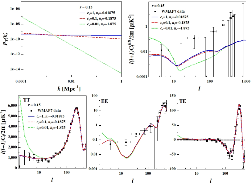
We firstly clarify how the different values of affect the shape of the angular power spectra of CMB.
In the upper-left panel of Fig. 1 we plot the primordial tensor power spectrum for =1, 0.1 and 0.01 respectively. We see that has significant influence on the tilt of the power spectrum through the consistency relation . In particular, at the large scale (small ), the =0.01 and =0.1 models have much larger values of than that in the model with .
This effect is also visible in , , and power spectra, which is shown in the upper-right and lower panels of Fig. 1 (with lensing). In all figures we take and fix other parameters at their WMAP7 best-fit values. It is shown that the amplitude of the power spectrum for =0.1 is slightly larger than the =1 case (not evident), while for the =0.01 case the low- s are significantly larger. The panels indicate that the set of parameters , is inconsistent with the WMAP data. Thus, we expect a tight constraint on when is small.
4.2 Results of Fitting
Our results of fitting for different models with fixed are shown in Table 1.
| Data & Model | (95.4% CL) | (95.4% CL) | |||
|---|---|---|---|---|---|
| WMAP | – | ||||
| – | |||||
| – | |||||
| WMAP+BICEP | – | ||||
| – | |||||
| – | |||||
| WMAP+BICEP | |||||
| (+) | |||||
Here we list the results for =1, 0.1 and 0.01. In the 4-9 rows, the constraints on , , and by using the WMAP+BICEP data are listed, divided into the and cases. For comparison, in the 1-3 rows we also list the results obtained by using the WMAP data alone with . We discuss the results of constraints in Sec. 4.2.1 and 4.2.2 in detail.
4.2.1 The case
In this subsection we briefly discuss the fitting results of models without including as a free parameter.
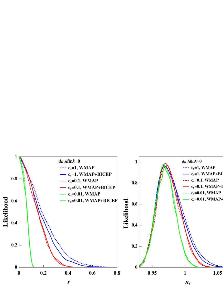
Let us first see the constraints on the tensor-to-scalar ratio which determines the amplitude of the tensor power spectrum. The fitting results of are listed in the second column of Table 1 and the likelihood functions are plotted in the left panel of Fig. 2. Using the WMAP data alone, we find a 95.4% CL constraint , which is well consistent with the result obtained by the WMAP 7-yr data (). As expected, we find the constraint on becomes much tighter if the value of becomes smaller (see the left panel of Fig. 2). Using the WMAP+BICEP data, we find and (95.4% CL) for and , respectively. This result is quite reasonable. According to the consistency relation , if is small, a large would lead to a large , leading to a large tensor mode on superhorizon scale, which is strongly constrained by low- CMB data. The necessary condition for inflation Eq. (12) is automatically satisfied by the constraint. The , case shown in the Fig. 1 is excluded.
Except for , another interesting issue is the fitting results of the scalar spectral index . Using the WMAP+BICEP data, we find , and (68.3% CL) for and . All the results are consistent with Harrison-Zeldovich spectrum () at 68.3% CL. The likelihoods of in different cases are plotted in the middle panel of Fig. 2. Similar to , we find that the upper bound constraint on also becomes tighter when is smaller. This effect is caused by the positive correlation between and . In the right panel of Fig. 2, we plot the marginalized contours in the plane, which shows that the smaller is, the tighter constraints on and .
The results of constraints from BICEP data are as follows. For the =1 model, we get (95.4% CL) by using the WMAP(WMAP+BICEP) data. The inclusion of BICEP data slightly improves the constraint by . However, for the and cases, since the constraints on mainly come from constraints on by the low- WMAP data, the inclusion of BICEP data does not lead to significant improvement in the result 777The Two-Year BICEP data, which maps only of the sky, measures limited modes of perturbations, therefore does not contribute too much on the total constraining.. The BICEP data can only affect through its correlation between , so it does not have significant effect on the results of .
4.2.2 The case
We now discuss the results of constraints with running of spectral index as a free parameter.
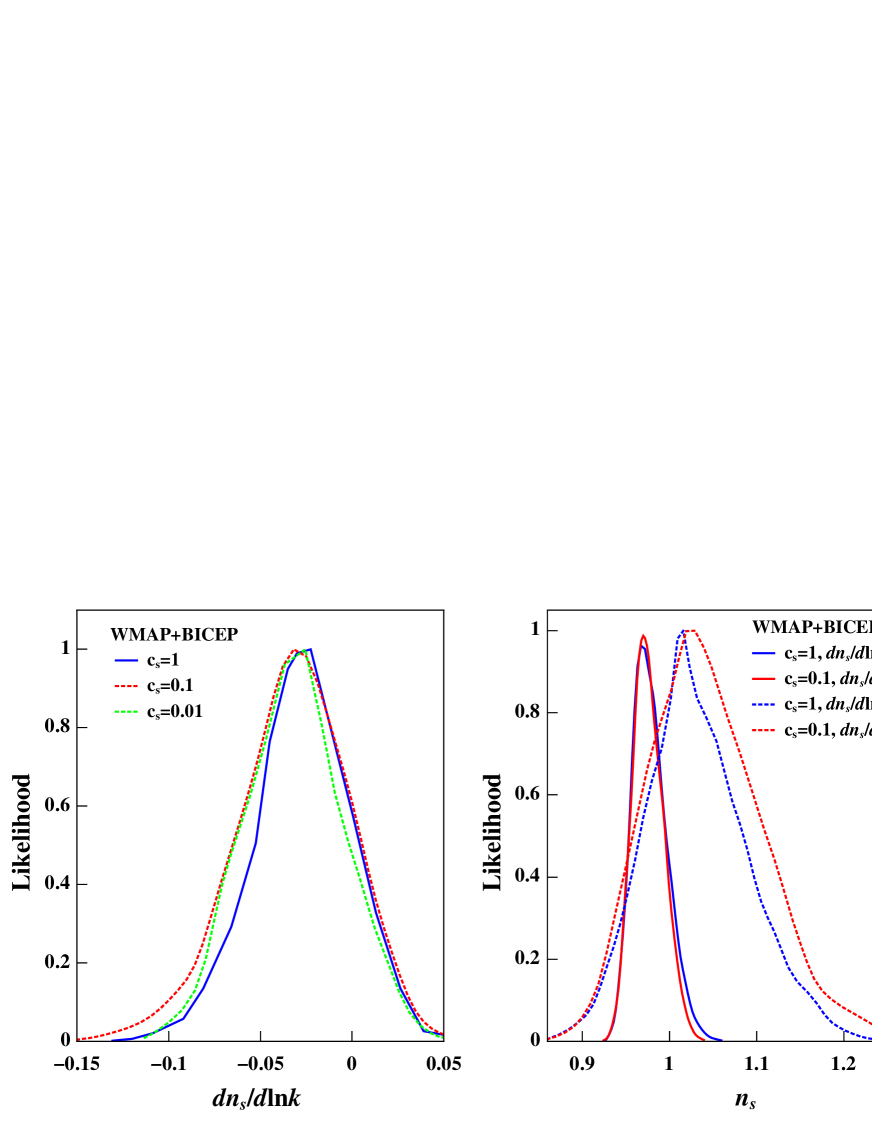
The fitting results are shown in the last three rows of Table 1 and Fig. 3. For the three models we find similar constraints on , thus does not have too much influence on .
The most striking effect of the inclusion of is the significant amplification of the allowed region of . In the middle panel of Fig. 3, we plot the likelihood functions of for (solid) and (dotted). We see that the width of likelihood is increased by nearly a factor of two. The inclusion of also changes the central values of from below 1 to above 1. These phenomena are caused by the strong anti-correlation between and (see the right panel of Fig. 3).
The inclusion of slightly releases the upper bound constraints of . For the , models, the 95.4% CL upper bounds on are 0.32, 0.26, 0.09 for and 0.36, 0.35, 0.10 for .
5 Cosmological Constraints of Free Models
In this section we consider the more general case, i.e., treating as a free parameter. 888We sample in the range of (0.001,1). We not only use the WMAP and BICEP power spectrum data, but also take and into consideration in order to constrain . A summary of the fitting results, including , , , and are given in Table 2. Notice that the word ‘UCON’ represents for ‘unconstrained’.
| Data & Model | (95.4% CL) | (95.4% CL) | ||||
|---|---|---|---|---|---|---|
| WMAP | UCON | – | ||||
| + | UCON | |||||
| WMAP+BICEP | UCON | – | ||||
| + | UCON | |||||
| WMAP+BICEP+ | – | |||||
| + | ||||||
5.1 Results of fitting Without Prior
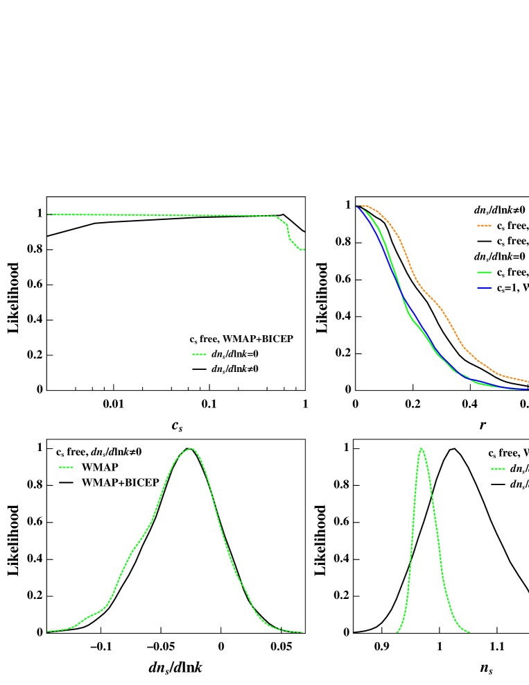
In this subsection we discuss the results obtained by WMAP+BICEP data, without adding and priors into the analysis. The fitting results of parameters are shown in the 1-4 rows of Table 2, and the likelihoods of , , and are plotted in Fig. 4.
Let us first have a look at the constraint on , and its likelihood is plotted in the upper-left panel of Fig. 4. The current CMB power spectrum data is not able to constrain on , and the likelihood function shows that it can take any possible value given the current constraints.
Secondly, the likelihoods of are shown in the upper-right panel of Fig. 4. We see the green and blue lines are close to each other, which means that the constraint on with free is similar to the result for =1. 999A similar conclusion was obtained in [17]. We get (95.4% CL) for both and free models (WMAP+BICEP, ). The inclusion of BICEP data slightly improves constraint of from 0.36 to 0.32 (). We see the inclusion of as a free parameter boardens the width of distribution of . At CL, the constraint is widened from to (WMAP+BICEP).
Thirdly, in the lower panels of Fig. 4 we plot the marginalized likelihoods of (left) and (right). We find that the results are similar to the fixed models. It implies that the BICEP data almost does not affect the constraint of , and the inclusion of greatly amplifies the distribution of and shifts its central value to above 1.
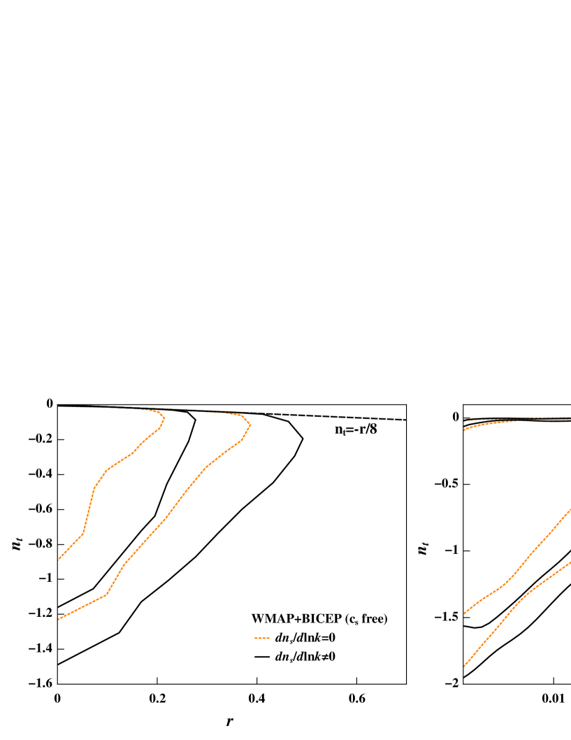
In addition, in Fig. 5 we plot the marginalized 2D-contours in the (left) and (right) planes. The slow-roll model with is plotted in the black dashed line in the left panel, and the and cases are shown in orange dotted and black solid lines, respectively. By releasing as a free parameter, ranges to much smaller values (-1 to -1.5 at 95.4% CL), especially in the small region. We find is still satisfied by the constraints. In both panels we see the inclusion of boardens the ranges of the parameter space.
5.2 Results of fitting With Prior
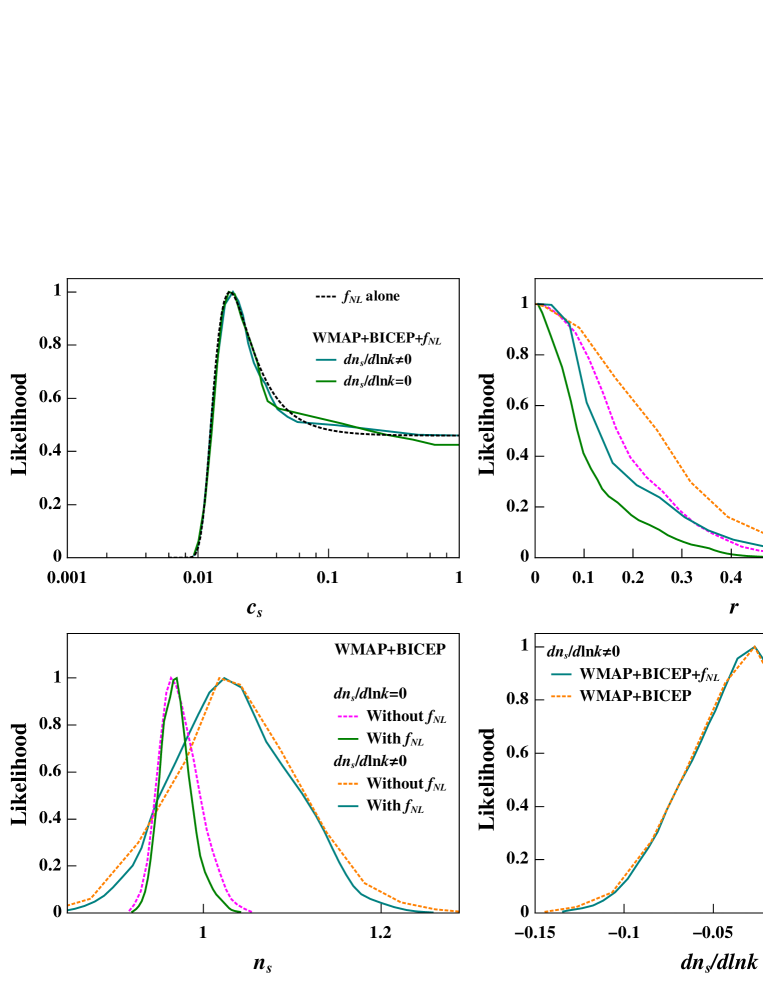
In this subsection let us take the and priors into account. The fitting results are shown in the last two rows of Table 2, and the likelihoods of , , and are plotted in Fig. 6.
The most striking effect is that the inclusion of and significantly improves the constraint on . At 68.3% CL, we obtain and for the cases of without and with as a free parameter. We find the large region, including the SFSR inflation with , is slightly disfavored at around 68.3% CL, while is excluded at 99.7% CL. Thus, the bispectrum data is much more powerful than the power spectrum data for constraining .
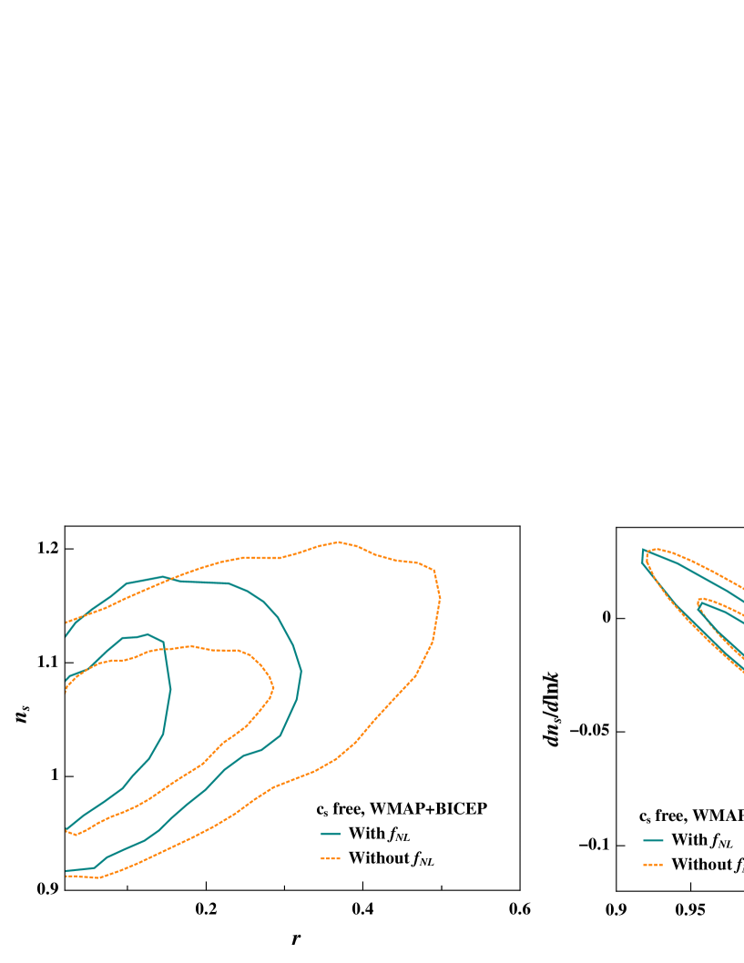
By narrowing the allowed range of , the addition of and also has interesting effect on constraining the other parameters. The likelihood of is shown in the upper-right panel of Fig. 6. We see that, once and priors are considered, the constraint becomes much tighter. This can be also seen through the contours in the left panel of Fig. 7. Again, due to the correlation between and , where and priors are included a slightly tighter constraint on the upper bound of is also obtained (see the lower-left panel of Fig. 6). But the effect of and priors on is negligible (see the lower-right panels of Fig. 6).
Finally, the correlations between , and are shown in Fig. 7. The left panel shows the contours and the right panel shows the contours. In all figures we set , as free parameters and use both WMAP and BICEP data. The cases of without and with as a free parameter are shown in orange and dark cyan colors. One can see the strong correlation between and , which suggests that if the distribution of is tightened, distribution is also constrained. However, the distribution of running spectral index , is not much affected by this correlation, because the change of is much smaller comparing with .
6 Conclusion
In this paper we make a detailed investigation of the cosmological interpretation of the consistency relation from CMB data. We focus on the general single-field inflation model in which the spectral index of tensor perturbation power spectrum is related to the tensor-to-scalar ratio by , and further investigate the effect of the sound speed . The datasets used in this paper include the WMAP power spectrum data, the BICEP -mode polarization data, and and priors obtained from the WMAP5 bispectrum data.
We discuss three models with fixed =1, 0.1 and 0.01. We find that when is small, the tilt of the tensor power spectrum becomes very large if is not too small, and then a tight constraint on is obtained for . Using the WMAP+BICEP data, we obtain the 95.4% CL constraints of 0.37, 0.26, 0.09 for the =1, 0.1, 0.01 cases (). Due to the positive correlation between and , smaller values of lead to slightly tighter constraint on the upper bound of . The effect of on the running of scalar spectral index is not obvious. The inclusion of significantly alters the constraints of , and slightly amplifies the upper bound constraint of .
For more general cases in which is taken as a free parameter, we find that unconstrained if we only use the current CMB power spectrum data in the analysis, and the marginalized distribution of , and are all similar to the case. However, after taking and priors into consideration, we find the sound speed is effectively constrained. The region is ruled out, and the region is disfavored at the 68.3% CL. From the constraints on , the inclusion of leads to tighter constraint on the and . In the case, we find (95.4% CL) with/without prior (), and the results for the case is . The running of spectral index is almost unaffected.
To summarize, we find that the consistency relation has significant effect in the constraints on cosmological parameters and when is small, while the parameter remains unaffected. Although the sound speed is unconstrained by the CMB power spectrum data, it can be effectively constrained by the CMB bispectrum data. Using the and priors obtained from the WMAP5 data, we find the SFSR model with =1 is slightly disfavored at the 68.3% CL. Thus, we are expecting that, the on-going and upcoming CMB observations, such as Planck [18] and CMBPol [19], with much lower instrumental noise and better foreground clean, will provide stronger constraints on inflation models.
Acknowledgments
QGH is supported by the project of Knowledge Innovation Program of Chinese Academy of Science and a grant from NSFC (grant NO. 10975167). The MCMC is mainly performed by the Lenovo Shenteng 7000 supercomputer in the Supercomputing Center of Chinese Academy of Sciences (SCCAS). XDL acknowledge the Institute of Theoretical Physics and the Supercomputing Center of USTC for the use of computing resources.
References
- [1] S. Weinberg, (Oxford University Press, New York, 2008).
- [2] A. H. Guth, Phys. Rev. D 23, 347 (1981); A. D. Linde, Phys. Lett. B 108, 389 (1982); D. H. Lyth and A. Riotto, Phys. Rep. 314, 1 (1999).
- [3] C. L. Bennett et al., Astrophys. J. Suppl. 148, 1 (2003); G. Hinshaw et al., Astrophys. J. Suppl. 170, 288 (2007); E. Komatsu et al., Astrophys. J. Suppl. 192, 18 (2011).
- [4] M. L. Brown et al., Astrophys. J. 705, 978 (2009).
- [5] H. C. Chiang et al., Astrophys. J. 711, 1123 (2010).
- [6] J. Kovac et al., Nature (London) 420, 772 (2002); A. C. S. Readhead et al., Science 306, 836 (2004); C. Bischoff et al. (CAPMAP Collaboration), Astrophys. J. 684, 771 (2008); W. C. Jones et al., Astrophys. J. 647, 823 (2006); J. H. P. Wu et al., Astrophys. J. 665, 55 (2007).
- [7] L. Knox, Phys. Rev. D 60, 103516 (1999). H. V. Peiris et al., Astrophys. J. Suppl. Ser. 148, 213 (2003); S. Chongchitnan and G. Efstathiou, Phys. Rev. D 73, 083511 (2006); L. Verde, H. Peris and R. Jimenez, JCAP 0601, 019 (2006); D. Baumann et al., AIP Conf. Proc. 1141, 10 (2009); Y. Z. Ma, W. Zhao and M. L. Brown, JCAP 1010, 007 (2010); M. J. Mortonson, H. V. Peiris and R. Easther, Phys. Rev. D 83, 043505 (2011).
- [8] W. Zhao and Q. -G. Huang, Class. Quantum Gravget. 28, 235003 (2011).
- [9] E. Komatsu et al., Astrophys. J. Suppl. 192, 18 (2011).
- [10] E. Komatsu et al., Astrophys. J. Suppl. 180, 330 (2009); K. M. Smith, L. Senatore and M. Zaldarriaga, JCAP 0909, 006 (2009).
- [11] L. Senatore, K. M. Smith and M. Zaldarriaga, JCAP 01, 028 (2010).
- [12] J. Garriga and V. F. Mukhanov, Phys. Lett. B 458, 219 (1999).
- [13] X. Chen, M. -x. Huang, S. Kachru and G. Shiu, JCAP 0701, 002 (2007).
- [14] Q. -G. Huang, JCAP 1005, 016 (2010).
- [15] A. Lewis, Phys. Rev. D 70, 043011 (2004); A. Lewis, A. Challinor and A. Lasenby, AJ 538, 473 (2000); http://www.camb.info
- [16] A. Lewis and S. Bridle, Phys. Rev. D 66, 103511 (2002); http://cosmologist.info/cosmomc/
- [17] Z. -K. Guo and D. J. Schwarz, Phys. Rev. D 81, 123520 (2010).
- [18] Planck Collaboration, The Scientific Programme of Planck [astro-ph/0604069].
- [19] D. Baumann et al., AIP Conf. Proc. 1141, 10 (2009).