Accurate and Efficient Private Release of Datacubes
Abstract
A central problem in releasing aggregate information about sensitive data is to do so accurately while providing a privacy guarantee on the output. Recent work focuses on the class of linear queries, which include basic counting queries, data cubes, and contingency tables. The goal is to maximize the utility of their output, while giving a rigorous privacy guarantee. Most results follow a common template: pick a “strategy” set of linear queries to apply to the data, then use the noisy answers to these queries to reconstruct the queries of interest. This entails either picking a strategy set that is hoped to be good for the queries, or performing a costly search over the space of all possible strategies.
In this paper, we propose a new approach that balances accuracy and efficiency: we show how to improve the accuracy of a given query set by answering some strategy queries more accurately than others. This leads to an efficient optimal noise allocation for many popular strategies, including wavelets, hierarchies, Fourier coefficients and more. For the important case of marginal queries we show that this strictly improves on previous methods, both analytically and empirically. Our results also extend to ensuring that the returned query answers are consistent with an (unknown) data set at minimal extra cost in terms of time and noise.
1 Introduction
The long-term goal of much work in data privacy is to enable the release of information that accurately captures the behavior of an input data set, while preserving the privacy of individuals described therein. There are two central, interlinked questions to address around this goal: what privacy properties should the transformation process possess, and how can we ensure that the output is useful for subsequent analysis and processing? The model of Differential Privacy has lately gained broad acceptance as a criterion for private data release [7, 9]. There are now multiple different methods which achieve Differential Privacy over different data types [1, 2, 4, 6, 11, 12, 14, 16, 17, 23]. Some provide a strong utility guarantee, while others demonstrate their utility via empirical studies. These algorithms also vary from the highly practical, to taking time exponential in the data size.
The output of the data release should be compatible with existing tools and processes in order to provide usable results. The model of contingency tables is universal, in that any relation can be represented exactly in this form. That is, the contingency table of a dataset over a subset of attributes contains, for each possible attribute combination, the number of tuples that occur in the data with that set of attribute values. In this paper, we call such a contingency table the marginal of the database over the respective subset of attributes. The set of all possible marginals for a relation is captured by the data cube. Contingency tables and the data cube in turn are examples of a more general class of linear queries, i.e., each query is a linear combination of the entries of the contingency table over all attributes in the input relation.
There has been much interest in providing methods to answer such linear queries with privacy guarantees. In this paper, we argue that these all fit within a general framework: answer some set of queries over the data (not necessarily the set that was requested), with appropriate noise added to provide the privacy, then use the answers to answer the given queries A limitation of prior work is that it applies uniform noise to the answers to : the same magnitude of noise is added to each query. However, it turns out that the accuracy can be much improved by using non-uniform noise: using different noise for each answer, while providing the same overall guarantee. The main contribution of this paper is to provide a full formal understanding of this problem and the role that non-uniform noise can play.
Example. Figure 1(a) shows a table with 3 binary attributes , and As in prior work [16], we think of a database as an -dimensional vector , where is the domain size of i.e., if has attributes then We linearize the domain of , so that each index position , , corresponds to a unique combination of attribute values, and is the number of tuples in that have values . In Figure 1(a), we linearized the domain in the order Here, position corresponds to the combination of values . Thus, since contains two tuples (1 and 4) with these values.
| : |
|
|||||||||||||||||||||||||
|---|---|---|---|---|---|---|---|---|---|---|---|---|---|---|---|---|---|---|---|---|---|---|---|---|---|---|
| = (1,2,0,1,0,0,1,0) |
| = |
| = |
| = |
Suppose that we want to compute two marginals over : the marginal over , and the marginal over . The query marginals can be represented as a matrix , as depicted in Figure 1(b), so that the answer is : The first two rows compute the marginal over ; i.e., the first row is the linear query that counts all tuples with ; while the second row counts all tuples with Similarly, the third row counts all tuples with and , and so on. Differentially private mechanisms answer in the form of , where is a random vector whose distribution provides a certain level of privacy. The error of the answer is generally defined as the variance [16, 23].
For example, one way to provide -differential privacy adds uniform noise to each answer. Based on the structure of in Figure 1(b), we can add noise with variance to each answer; see details in Section 2). Over the six queries, the sum of variances is . However, we can do better with a non-uniform approach. For example, we can add noise with variance to the answers for the first two rows of , and noise with variance to the remaining four answers, and still provide -differential privacy. The sum of the six variances is then . We can improve this even further by changing how we answer the queries: we can answer the first query by taking half of the first answer, and adding half of the third and fourth answers. The resulting variance of is
Similar tricks yield the same variance for all other answers, so the sum of all six variances is now , a 28% reduction over the uniform approach. ∎
This example shows that we can significantly improve the accuracy of our answers while preserving the same level of privacy by adopting non-uniform noise and careful combination of intermediate answers to give the final answer. Yet further improvement can result by choosing a different set of queries to obtain noisy answers to. The problem we address in this paper is how to use these techniques to efficiently and accurately provide answers to such queries that meet the differential privacy guarantee. This captures the core problems of releasing data cubes, contingency tables and marginals. Our results are more general, as they apply to arbitrary sets of linear queries , but our focus is on these important special cases. We also discuss how to additionally ensure that the answers meet certain consistency criteria. Next, we study how existing techniques can be applied to this problem, and discuss their limitations.
The Strategy/Recovery approach. Mechanisms for minimizing the error of linear counting queries under differential privacy have attracted a lot of attention. Work in the theory community [2, 10, 11, 12, 13, 22] has focused on providing the best bounds on noise for an arbitrary set of such queries, in both the online and offline setting. However, these mechanisms are rarely practical for large databases with moderately high dimensionality: they can scale exponentially with the size of their input.
Work in database research has aimed to deliver methods that scale to realistic data sizes. Much of this work builds on basic primitives in differential privacy such as adding appropriately scaled noise to a numeric quantity from a specific random distribution (see Section 2). Repeating this process for multiple different quantities, and reasoning about how the privacy guarantees compose, it is possible to ensure that the full output meets the privacy definition. The goal is then to minimize the error introduced into the query answers (as measured by their variance) while satisfying the privacy conditions.
Given this outline, we observe that the bulk of methods using noise addition fit into a two-step framework that we dub the ‘strategy/recovery’ approach:
-
•
Step 1. Find a strategy matrix and compute the vector , where is a random noise vector drawn from an appropriate distribution. Then is the differentially private answer to the queries represented by .
-
•
Step 2. Compute a recovery matrix , such that . Return as the differentially private answer to the queries The variance is often used as an error measure for the approach.
We show this method schematically in Figure 2. For example, Figures 1(c) and 1(d) show a possible choice of matrices and for the query matrix in Figure 1(b). In this case, the strategy computes the marginal on ; Step 1 above adds random noise independently to all cells in this marginal. The recovery computes the marginal on by aggregating the corresponding noisy cells from the marginal on (the first two rows of ), and also outputs the marginal on (the last four rows of ).
We now show how prior work fits into this approach. In many cases, the first step directly picks a fixed matrix for , by arguing that this is suitable for a particular class of queries . For example, when setting (hence ), the approach computes a set of noisy counts by adding Laplace noise independently to each . The answer to any query matrix is computed over these noisy counts, i.e., ; this model was analyzed in [1]. By contrast, when (and ), as discussed in [7], the approach adds noise to the result of each query in , i.e., .

Several more sophisticated strategies have been designed, with the goal of minimizing the error for various query workloads. When consists of low-dimensional range queries, [23] proposes to be the wavelet transform, while [14] studies the strategy corresponding to a hierarchical structure over . However, as shown in [16], neither of these strategies is particularly accurate for other types of queries. For marginals, [1] chooses to be the Fourier transform matrix, and [6] employs a clustering algorithm over the queries to compute . Figures 1(c) and 1(d) depict the output computed via [6] on query matrix (Figure 1(b)). Other work has suggested the use of random projections as the strategy matrix, connecting to the area of sparse recovery [5, 18]. Many of these choices are relatively fast: that is, and can be applied to a vector of length in time or in the case of wavelet and Fourier transforms, respectively. This is important, since real data can have large values of , and so asymptotically higher running time may not be practical. A limitation of [6] is that the clustering step is very expensive, limiting the scalability of the approach.
An important technical distinction for the strategy/recovery approach is whether or not the strategy is invertible. If it is (e.g., when is the Fourier or wavelet transform), then the recovery matrix is unique, and the query answer is guaranteed to be consistent (see Definition 2.3). Then the error measure depends only on (and ). However, if is not invertible, then there can be many choices for , and depends on both and . The optimal recovery that minimizes (for a fixed ) can be computed via the least squares method [14, 16] and has a closed-form expression as a function of . Using this fact, Li et al. [16] study the following optimization problem: Given queries and a formula for as a function of , compute the strategy that minimizes . This is a tough optimization, since the search is over all possible strategy matrices . Their matrix mechanism uses a rank-constrained semidefinite program (SDP) to compute the optimal . Solving this SDP is very costly as a function of , making it impractical for data with more than a few tens of entries.
In summary, the search for a strategy matrix is currently done either by picking one that we think is likely to be “good” for queries , or by solving an SDP, which is impractical even for moderate size problems.
Our Contributions. Most of the prior approaches discussed above use the uniform “noise budgeting” strategy, i.e., each value of the noise vector is (independently) drawn from the same random distribution. The scaling parameter of this distribution depends on the desired privacy guarantee , as well as the “sensitivity” of the strategy matrix (see Section 2).
In the extended version of [16], the authors prove that any non-uniform noise budgeting strategy can be reduced to a uniform budgeting strategy by scaling the rows of with different factors. However, computing the optimal scaling factors this way is impractical, as it requires solving an SDP. The only efficient method for computing non-uniform noise budgets we are aware of applies to the special case when is a range query workload [4]. There, corresponds to a multi-dimensional hierarchical decomposition, and recovery corresponds to the greedy range decomposition. The resulting budgeting is not always optimal.
In this paper we show how to compute the optimal noise budgets in time at most linear in the sizes of and , for a large class of queries (including marginal queries), and for most of the matrices considered in prior work. This includes the Fourier transform, the wavelet transform, the hierarchical structure over , and any strategy consisting of a set of marginals (in particular, the clustering strategy of [6]).
The overall framework introduced is depicted in Figure 3: Given strategy matrix and recovery matrix , we compute optimal noise budgets for each query, and draw each noise value from a random distribution that depends on (Step 2). We then derive a new recovery matrix that minimizes (Step 3), for the noise budgets computed in Step 2.

The most general approach would be to provide a mathematical formulation for the following global optimization problem: Given the query matrix , compute the strategy , the recovery , and the noise budgets that minimize . However, this problem essentially reduces to that addressed by the matrix mechanism [16], and requires solving an SDP.
Instead, we study how to efficiently solve optimization problems where two out of the three parameters , and are fixed. In Section 3.1, we solve the optimization problem: Given a decomposition of query matrix into strategy and recovery , compute the optimal noise budgets that minimize . We provide a formula for , as a function of and . In Section 3.2, we apply the generalized least squares method to solve the following problem: Given the query matrix , the strategy , and the noise budgets , compute the recovery that minimizes . Following the steps in this framework provides efficient algorithms with low error. A faster alternative computes a consistent output of Step 3 with small (but non-optimal) error; see Sections 3.3 and 4.3. Our approach strictly improves over the previous result from [6].
In the common case that is invertible, our framework decreases the error for the Fourier and wavelet approaches from prior work. Computing the optimal noise budgets here is very fast, so this improvement comes with only a small time overhead: less than 1 second in our experiments.
To summarize, our contributions are as follows:
-
•
We propose a framework for minimizing the error of differentially private answers. It improves on the accuracy of existing strategies, at minimal computation cost.
-
•
We develop fast algorithms within this framework for marginal queries. Our algorithms compute consistent answers. In particular, when is the set of all -way marginals, we give asymptotic bounds on the error of our mechanism; we are not aware of any such analysis for the matrix mechanism. As a by-product, our analysis also improves the error bound for the uniform noise case.
- •
Organization. Section 2 introduces the necessary definitions for describing our framework. The optimization results required by Steps 2 and 3 are developed in Section 3. In Section 4, we describe novel results that allow us to apply our framework to marginal queries in an efficient manner, and to compute consistent results. Our experimental study is presented in Section 5, and we conclude in Section 6.
2 Definitions
We begin by recalling the definition of differential privacy and some fundamental mechanisms which satisfy this definition.
Definition 2.1 (Differential privacy [9, 8]).
A randomized algorithm satisfies -differential privacy if for all databases and differing in at most one element, and all measurable subsets ,
We say that an algorithm satisfies -differential privacy if it satisfies -differential privacy.
Definition 2.2 (-sensitivity).
For let the -sensitivity of a function be defined as:
for all and differing in at most one element. Here, denotes the standard norm, i.e., for .
We rely on the following two basic mechanisms to construct differentially private algorithms:
Theorem 2.1 (Laplace mechanism [9]).
If is a function , then releasing with additive -dimensional Laplace noise with variance in each component satisfies -differential privacy.
Theorem 2.2 (Gaussian mechanism [8, 19]).
If is a function , then releasing with additive -dimensional Gaussian noise with variance in each component satisfies -differential privacy.
Query workloads, consistency, strategy and recovery. As mentioned in Section 1, we represent the database as a vector and the query workload as a matrix : each row , is a linear query over database It is easy to see that the sensitivity of is where denotes the th column of .111We assume that each individual contributes a weight of 1 to some entry of , in line with prior work. Other cases can be handled by rescaling the sensitivity accordingly. One differentially private answer to is a vector , where is the noise vector drawn from an appropriate (Laplace or Gaussian) distribution. Our formal goal is to minimize the variance of a given linear functional for some fixed vector , while guaranteeing differential privacy. For example, if we minimize the sum of the variances of noise over all queries. In particular, we study workloads that consist of marginals over , such as the set of all -way marginals, for some small integer .
Definition 2.3.
A noisy output is consistent if there exists at least one vector such that
We decompose a query workload into a strategy matrix , and a recovery matrix , such that . The query answer is then computed as , where is the noisy answer to (hence, ). In general, there are many possible ways to pick and given , and our goal will be to minimize the resulting
3 Our Framework
In this section we solve the optimization problems required by Steps 2 and 3 of our framework from Figure 3.
3.1 Optimal Noise Budgeting (Step 2)
A novel part of our scheme is a special purpose budgeting mechanism: For each row in the strategy , we release , where is drawn from a Laplace distribution that depends on a value . We show how to choose the values optimally so that the overall method satisfies -differential privacy and the resulting noise is minimized. We also design an approach based on grouping rows of the strategy matrix , which allows us to compute the optimal ’s efficiently.
Proposition 3.1.
Let be an strategy matrix, and let be a set of non-negative values. Define the noisy answer to to be an -dimensional vector such that ,
(i) If is drawn from the Laplace distribution with variance then satisfies -differential privacy, where .
(ii) If is drawn from the Gaussian distribution with variance and , satisfies -differential privacy.
Proof.
We only show (i), the proof for (ii) is shown in A. We decompose as where is the diagonal matrix . We now consider the sensitivity of the function . From Definition 2.2, we have
Thus, adding noise with variance proportional to provides -differential privacy (via Theorem 2.1 with ) or -differential privacy (via Theorem 2.2 with ). Finally, multiplying by has the effect of rescaling the variance in each component: the th component now has variance proportional to . Setting for or and applying the correct scaling constants gives the claimed result. ∎
The proofs for (ii) and other results are omitted for brevity.
Recall that the output is computed as . Our goal is to choose values that minimize the variance We detail this for Laplace mechanism:
Let . By Proposition 3.1, it follows that the optimal noise budgeting is the solution to the following optimization problem:
| Minimize: | (1) | |||
| Subject to: | (2) | |||
| (3) |
Because all ’s are non-negative, the objective function is convex. The body defined by the linear inequalities is also convex. The resulting problem can thus be solved using a convex optimization package that implements, e.g., interior point methods. Such methods require time polynomial in , and the required accuracy of the solution [21].
Efficient Solution via Grouping. Convex optimization solvers may require a large number of iterations and be too inefficient for databases of moderate dimensionality. However, for most of the frequently used strategy matrices, the optimization problem can be significantly simplified, if we partition the rows of the strategy matrix into groups, and define the corresponding values to be the same for all rows in a group. We show that the groups can be chosen in such way that all conditions become identical once we set the ’s to be equal in each group, which leads to a closed form solution. This approach was implicitly used in [4]. We show that this concept can be applied to a larger class of strategy matrices. The optimal solution for the simplified problem is a feasible solution for the general problem. If recovery matrix satisfies a certain property (as is the case for all matrices we consider), then the optimal solution for the simplified problem is also guaranteed optimal for the general case. In particular, we find optimal noise budgets for strategy/recovery methods such as Fourier [1] and clustering [6].
Definition 3.1.
Let be an strategy matrix. We say that satisfies the grouping property if there exists a grouping function over its rows , , such that the following two conditions are satisfied:
— row-wise disjointness: for any two rows of with and for any column ,
— bounded column norm: for any group , and for any two columns , we have
The minimum for which has a grouping function is called the grouping number of .
Together, the two conditions in Definition 3.1 imply that any column of contains at most one non-zero value from each group, and that that value is the same (within a group) for all columns. Hence, not every can meet this definition: while we could put every row in a singleton group, we also then require that the magnitude of all non-zero entries in the row are identical. Nevertheless, as we show below, many commonly used matrices are groupable.
Example. Matrix in Figure 1(c) has grouping number : each column has exactly one entry equal to 1, so . On the other hand, if is the matrix in Figure 1(b), the grouping number is 2: we define one group containing the first two rows, and another containing the last four rows. We have Note that, e.g., the first and third rows cannot be grouped together, since We now apply this definition to the other strategy matrices proposed:
Base counts. As noted in the introduction, directly materializing the noisy version of is equivalent to In this case, all rows form a single group; hence, and .
Collections of marginals. When is a set of marginals, all rows that compute the cells in the same marginal can be grouped together, as in the above example. Hence, the number of groups is the number of marginals computed; and for each group .
Hierarchical structures. When represents a hierarchy over , all rows that compute the counts at the same level in the hierarchy form one group. Hence, the grouping number is the depth of the hierarchy and all values are 1. Specifically, when represents a binary tree over , the grouping number is The same essentially holds for the one-dimensional Haar wavelet (here, ). For higher dimensional wavelets, the grouping number grows exponentially with the dimension of the wavelet transform.
Fourier transform. The Fourier transform (discussed in more detail in Section 4.1) is dense: every entry is non-zero and has absolute value . In this case, each row forms its own group, the grouping number is , and for any group .
Sparse random projections. Sketches are sparse random projections that partition the data into buckets, repeated times [5]. All entries in the sketch matrix are . In this case, all rows that define one particular partition of the data form one group, so and .
Arbitrary strategies . If is groupable, we can greedily find a grouping as follows: start a group with an arbitrary row, and try to add each remaining row to existing groups; if a row cannot be added to an existing group, a new group is created for it. While this may not result in a minimum , any grouping suffices for our purposes. We do not discuss the greedy approach further, since all the strategies we study can be grouped directly as discussed above.
Definition 3.2.
Let be an strategy matrix with grouping function . Let be a corresponding recovery matrix. We say that is consistent with if for any rows of with , we have (where are as in objective function (1)).
When is a set of marginals and it is easy to verify that is consistent with the optimal grouping of , for all the choices of considered in prior work: , , Fourier transform, and strategy marginals computed by clustering [6] (here, aggregates cells of the centroid marginal to compute each of the marginals assigned to a cluster).
The next result follows directly from the properties of the grouping function.
Lemma 3.2.
Proof.
Let be the noise budgets corresponding to the groups of ; i.e., all values for the rows in group 1 are equal to , etc. Because of the grouping property, each condition (2) becomes where is the value defined by the bounded column norm for the group (recall Definition 3.1). Since the objective function is a minimization, we can make this inequality an equality. Clearly, are a feasible solution for (1) – (3).
Thus, when has grouping function , we can write a simpler optimization problem for noise budgeting:
| Minimize: | (4) | |||
| Subject to: | (5) | |||
| (6) |
Since there is now just a single constraint on the s, we can solve this via a simple Lagrange multiplier method. The corresponding Lagrange function is:
Setting the partial derivatives to zero, we obtain By the privacy constraint (5), and thus:
Corollary 3.3.
In the case when all values are equal to the same value the optimum value of the objective function is equal to , where . For -differential privacy the corresponding value of the objective function is equal to .
Lemma 3.2 implies the following.
Theorem 3.4.
As discussed above, when is a set of marginals, all the strategy/recovery matrices proposed in prior work fit the conditions of Theorem 3.4, and thus their accuracy can be improved via optimal noise budgeting. Observe that the optimization problem (4) – (6) can be solved reasonably fast: given , and a grouping of , we can derive the vector of values in time linear in the size of , i.e., in . For particular (e.g. the Fourier matrix), the cost can be even lower, due to the symmetric structure of and . Finally, all values, as well as , can be computed in time.
3.2 Optimal Recovery Matrix (Step 3)
Given and the noise parameters , we wish to compute a matrix such that and is minimized. Recall that , where is drawn from the Laplace distribution of variance , as in Section 3.1 (the case of Gaussian distribution is similar). As we show below, the resulting will also be consistent.
We derive via least squares statistical estimators. More precisely, given , we first compute an estimate of which is linear in and has minimum variance. The vector is called the optimal (generalized) least squares solution. As we show below, for some matrix . We then define and . A similar approach was used in [16] for the case of uniform noise. We extend the computation to the case of non-uniform noise budgets .
Let be the covariance matrix of : Define ; hence, For simplicity, we assume that . The same ideas as in [16, Section 3.3] can be used to handle the case ; see also [20] for further details. Then the LS solution is computed as
Since is diagonal, . We obtain
Let . We define , i.e.,
| (7) |
Note that is consistent, as per Definition 2.3 (with ). By a well-known result from linear statistic estimation [20], the following holds:
Lemma 3.5.
Matrix computed as in (7) minimizes (where ). Moreover, is consistent and unbiased, i.e., .
Observation 1.
If is an orthonormal basis (as with wavelets, Fourier and identity strategies), we have . This implies , so .
The cost of finding as above is relatively high, due to the need to perform matrix inversion. While the diagonal matrix is trivial to invert, since , the matrix is generally dense, so is more costly to invert.
3.3 Fast Consistency
The vector computed via the optimal recovery matrix in Step 3 (Section 3.2) has two important properties: (i) is consistent (Definition 2.3); and (ii) is minimized for each . Since we have . Thus, achieves minimum error for each query in expectation. As observed in [1, 6] for practical applications it may be necessary to return a vector which is consistent and minimizes a different error measure, e.g., we may wish to minimize For example, implies that minimizes the average error and minimizes maximum error.
In this section we show how to efficiently compute another recovery matrix such that is consistent and is small. This approach is particularly useful when the query matrix has . As we show below, we significantly improve the running times of the approaches used in [1, 6] for this case. The approach in [1, 6], translated in our strategy/recovery framework, is described below.
Start by defining a recovery matrix such that and has bounded error . Usually, is the recovery matrix from Step 2 of our framework. For example, the matrix in [6] is implied by the clustering function over marginals, which heuristically minimizes some -error of the noisy answers. Next, compute a consistent answer that minimizes . Recall that is consistent if there exists such that . Hence, for or , can be computed via a linear program (LP) with variables corresponding to the entries of , and consistency conditions expressed as linear constraints. Other requirements can also be imposed on , e.g., integrality or non-negativity. For , is the solution to a least squares problem (LS).
However, such an LP, resp. LS, uses at least variables corresponding to the entries in . When is large (as is usually the case), this leads to large linear programs. This issue was reported as a bottleneck in the experimental evaluation of [6]. We now propose a different LP, resp. LS, formulation for the consistency problem, which requires at most variables (recall that is the number of queries in the workload ). This leads to large improvements in running time when .
First, note that implies that any answer is consistent. This is because the linear system admits the solution ( implies that is invertible). In particular, is consistent and minimizes for any .
Assume that . We pick linearly independent rows of , denoted as , and use them to decompose as for some matrix . Because has linearly independent rows, the above argument implies that, for any , the linear system has a solution. Hence, any answer is consistent for the queries . Then is consistent for all queries : We find that minimizes and return : For and , is the solution to an LP; for , is the solution to a least squares problem. In all cases, the number of variables is . As observed in [1], the utility guarantee follows by the triangle inequality. If , then
Thus, the additional -error introduced by consistency is at most the -error of the original noisy answer, i.e., the error at most doubles.
When is a set of marginals, we can formulate the LP, resp. LS, without explicitly computing or finding a collection of linearly independent rows . Rather, we use the Fourier coefficients of the marginals. The discussion is deferred to Section 4.3.
4 Consistent Marginals via Fourier Strategies
In this section, we focus on the case when all queries correspond to marginals. Here, we show that the choice of as an appropriate Fourier matrix gives strong guarantees on the variance, as well as providing consistent query answers.
4.1 Marginals and Fourier analysis
In this section we assume that all attributes in the database table are binary; for simplicity, let the domain of each attribute be . We emphasize that this assumption is without loss of generality: an attribute which has distinct values can be mapped to binary attributes (and we do so in our experimental study). However, we present our results with binary attributes to avoid overcomplicating the notation. Consequently, there are entries in the database vector , where each entry is indexed by some , and is the number of entries in the database with attributes ; recall the example in Figure 1(a).
There are also possible marginals (a.k.a. subcubes of the data cube) of interest, corresponding to aggregations along a subset of dimensions. For any , let denote the marginal over non-zero attributes in , and let denote the number of non-zero entries in , i.e., the dimensionality of the marginal. Note that here is the bit-vector indicator for the attributes in the marginal. We will consistently use it as a superscript in such cases, and as a subscript when it indexes an entry in a vector.
We use the following notations, as in [1]: For any pair of we write for the bit-wise intersection of the pair, i.e. . The inner-product in this space, , can also be expressed via the intersection operator: . We say that is dominated by , denoted , if .
The computation of a marginal over the input can be thought of as a linear operator mapping the full-dimensional contingency table to the marginal over non-zero attributes in , by adding relevant entries over the attributes not in . More precisely, for each , the cell in the marginal , denoted , sums the entries in the contingency table whose attributes in are set to values specified by :
Example. Let be the vector in Figure 1(a). Assume we want to compute the marginal , i.e., the marginal over attributes and . Then the value in the cell is denoted by (i.e., ). The value in the cell is denoted by . Note that and . On the other hand, , so there is no cell in the marginal over . So, while the cell index is -dimensional, only the bits corresponding to non-zeros in vary—the rest are held at 0. Hence, there are only cell indexes in the marginal . In this example, there are only 4 cells in . By the above formula, and ∎
The set of all marginals with is referred to as the set of all -way marginals. They are commonly used to visualize the low-rank dependencies between attributes, to build efficient classifiers from the data, and so on.
We use the Hadamard transform, which is the -dimensional discrete Fourier transform over the Boolean hypercube . This allows us to represent any marginal as a summation over relevant Fourier coefficients. The advantage is that the number of coefficients needed for each marginal is just the number of entries in the marginal. The Fourier basis vectors for have components The vectors form an orthonormal basis in . We will use the following properties of Fourier basis vectors and marginal operators in the Fourier basis (proofs can be found in [1]):
Theorem 4.1.
For all we have:
-
1.
.
-
2.
| Strategy | -privacy | -privacy |
|---|---|---|
| Base counts | [9] | [8] |
| Marginals | [1] | [1] |
| Fourier coefficients (uniform noise) | Theorem B.1 | [1] |
| Fourier coefficients (non-uniform noise) | Lemma 4.2 | Lemma 4.2 |
| Lower bound | [15] | [15] |
4.2 Bounds for marginals
The use of a Fourier strategy matrix was studied in [1], under a uniform error budget. Here, we show that using a non-uniform budgeting can provide asymptotically improved results. We study the case when the query set corresponds to a collection of marginals . For a given marginal the accuracy bounds will be parametrized by its dimensionality , the total number of marginals and the total number of Fourier coefficients corresponding to the collection of marginals, denoted as . Theorem 4.1(2) implies that . If the random variable corresponding to the differentially private value of a marginal is denoted as , then we state a bound on the expected absolute error, to simplify presentation and comparison with prior work. All our bounds can also be stated in terms of the variance , or as high-probability bounds.
The asymptotic bounds on error are easier to interpret in the important special case of the set of all -way marginals. In this case because of the symmetry of the query workload, the expected error in all marginals is the same. Table 1 summarizes bounds on error in this case together with the unconditional lower bounds for all differentially private algorithms from [15]. While in the case of -differential privacy our upper bounds are almost tight with the lower bounds from [15], for -differential privacy the gap is still quite significant and remains a challenging open problem.
Our next lemma (proof in Appendix C) gives bounds on expected error of the Fourier strategy with non-uniform noise.
Lemma 4.2.
For a query workload consisting of all -way marginals over data the bounds on the
expected error of the Fourier strategy mechanism with non-uniform noise are given as follows:
1. For -differential privacy the expected noise per marginal is
.
2. For -differential privacy the expected noise per
marginal is .
These bounds are summarized in Table 1, along with those that follow from other approaches.We note in passing that we can provide a tighter analysis of the noise for the Fourier strategy under uniform noise than in [1], by a factor of —details are in Appendix B.
Time cost comparison. To directly compute a single -way marginal over -dimensional data takes time , and so computing all -way marginals takes naively. Computing the Fourier transform of the data takes time , and deriving the -way marginals from this takes time per marginal, i.e., for all marginals [1]. We compare the cost of different strategies to these costs. Materializing noisy counts () and aggregating them to obtain the -way marginals also takes time , as does materializing the marginals and then adding noise ().
The clustering method proposed in [6] is more expensive, due to a search over the space of possible marginals to output. The cost is : clearly as the dimensionality grows, this rapidly becomes infeasible. However, across all strategies, the step of choosing the non-uniform error budget is dominated by the other costs, and so does not alter that asymptotic cost.
4.3 Consistency via Fourier coefficients
In Section 3.3 we discussed a general approach for computing consistent answers for a query workload with . The approach required explicitly finding a set of linearly independent rows in and decomposing . We now show that when is a set of marginals we can compute consistent answers without such expensive steps. Instead, we ensure consistency by writing an LP that uses the Fourier coefficients corresponding to the marginals in . Let consist of marginals . We introduce variables for the Fourier coefficients corresponding to these marginals, denoted as . To simplify notation, we rename them as , where . Marginals can be computed from , using formulas from Theorem 4.1:
for all and . We will index entries in the marginals by pairs , where . Let the total number of entries in marginals be equal to . Let be the recovery matrix for the Fourier strategy: with entries . Then . Suppose that we are given a set of inconsistent noisy values of these marginals . We formulate the following optimization problem to find the consistent set of marginals that is closest to the noisy values in -norm:
For this is gives a least squares problem, with variables and constraints, which is expressed as:
For and , this gives an LP similar to [1].
The running time of this consistency step via least squares only depends on the number of queries. For example, for the case of all -way marginals, we need to work with matrices of size , and perform a constant number of multiplications and inversions. In contrast, prior work required solving LPs of size proportional to the size of the data, , which takes time polynomial in .
5 Experimental study
Datasets. We studied performance on two real datasets:
Adult: The Adult dataset from the UCI Machine Learning repository
(http://archive.ics.uci.edu/ml/) has census information
on 32561 individuals. As in [6], we extract
a subset of sensitive categorical attributes, for workclass
(cardinality 9), education (16), marital-status (7), occupation (15),
relationship (6), race (5), sex (2) and salary (2).
NLTCS: The National Long-Term Case Study from StatLib (http://lib.stat.cmu.edu/), contains information about
21576 individuals.
Each record consists 16 binary attributes, which correspond to
functional disability measures: 6 activities of daily living and 10
instrumental activities of daily living.
Query workloads.
The choice of query workloads in our experimental study is motivated
by an application of low-order marginals to statistical model
fitting.
In this setting, the typical set of queries consists of all -way marginals
(for some small value of ) together with some subset of
-way marginals, chosen depending on the application.
We consider three different approaches:
1. : all the -way marginal tables.
2. : all the -way marginal tables, plus half of all
-way marginals.
3. : all the -way marginal tables, plus all -way
marginals that include a fixed attribute.
Evaluation metrics. We measure the average absolute error per entry in the set of marginal queries. To show the utility of these results, we scale each error by the mean true answer of its respective marginal query, i.e., we plot it as a relative error. Thus, a relative error of less than 1 is desirable, as otherwise the true answers are dwarfed by the noise (on average). Note that while the number of tuples in each dataset is relatively small, our approaches do not depend on the tuple count, but rather the dimensionality of the domain Larger datasets would only improve the quality metrics, while keeping the running time essentially unchanged.
Algorithms Used. We present results for -differential privacy. Results for -differential privacy are similar, and are omitted. We include seven approaches within the strategy/recovery framework, based on choice of the strategy matrix, . Here, the notation indicates that we use the non-uniform noise allocation for strategy as described in Section 3.1, while the corresponding is with uniform noise.
-
•
— Add noise via Laplace mechanism directly to base cells and aggregate up to compute the marginals. Here, the optimal noise allocation is always uniform.
-
•
— Add uniform () or non-uniform () noise to each marginal independently.
-
•
— Add uniform () or non-uniform () noise to each Fourier coefficient, corresponding to the given query workload.
-
•
— Add uniform () or non-uniform () noise to each marginal returned by the greedy clustering strategy proposed in [6].
Our goal is to study the effects of non-uniform noise budgeting over all strategies. The decision on which strategy to use rests with the data owner. However, we show clear tradeoffs between running time and accuracy for all strategies, which can provide helpful hints.
To ensure consistency of the released marginals, we use the Fourier analytic approach, described in Section 4.3.
5.1 Adult Dataset
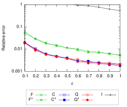
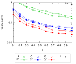
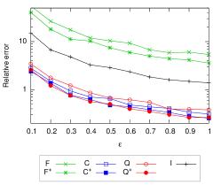
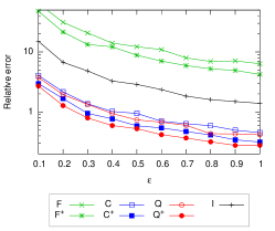
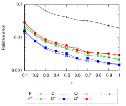
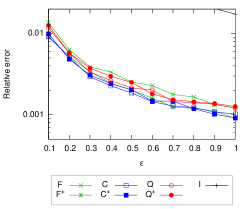
Figure 4 shows the results on the Adult data set, for query workloads and . The attributes in this data set have varying cardinalities, but are encoded as binary attributes as described in Section 4.1. We plot the results on a logarithmic scale as we vary the privacy parameter , to more clearly show the relative performance of the different measures. Immediately, we can make several observations about the relative performance of the different methods. On this data, the naive method of materializing counts () is never effective: the noise added is comparable to the magnitude of the data in all cases. Across the different query workloads, choosing the strategy works generally well. In this case non-uniform noise allocation can significantly improve the accuracy. For example, over workload (Figure 4(b)), we see an improvement of 20-25% in accuracy.
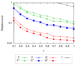
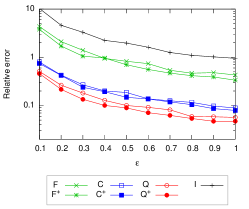
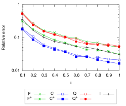
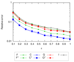
For more complex queries which result in more marginals of higher degree ( and , in Figures 4(e) and 4(f) respectively), the accuracy is lower overall, and the noise is greater than the magnitude of the data for more restrictive settings of the privacy parameter . To some extent this can be mitigated as the number of individuals represented in the data increases: the noise stays constant as the value of the counts in the table grows.
Across this data, we observe that while the non-uniform approach improves the accuracy of the Fourier strategy, it is inferior to other strategies. Although asymptotically this strategy has good properties (as described in Table 1), in this case is not very large, so the gap between the and terms for constant is absorbed within the big-Oh notation. The running times of our methods were all fast: the Fourier () and Query () methods took at most tens of seconds to complete, while the clustering () took longer, due to the more expensive clustering step.
5.2 NLTCS data
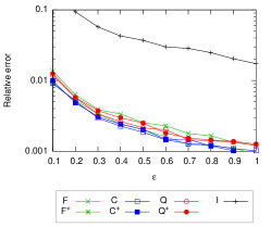
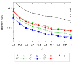
Figure 5 shows the corresponding results on the binary NLTCS data. Over all experiments, there is an appreciable benefit to applying the optimal non-uniform budgeting. The optimal budgeting case is reliably better than the uniform version, for the same strategy matrix. There are occasional inversions, due to the random nature of the mechanisms used, but the trend is clear. The advantage can be notable: for example, on (Figure 5(b)) and (Figure 5(e)), the error of the Fourier strategy is reduced 30-35% by using non-uniform budgeting. For the clustering approach, the improvement is smaller, but still measurable, around 5% on average. However, recall that strategy becomes infeasible on higher dimensional data, due to its exponential cost.
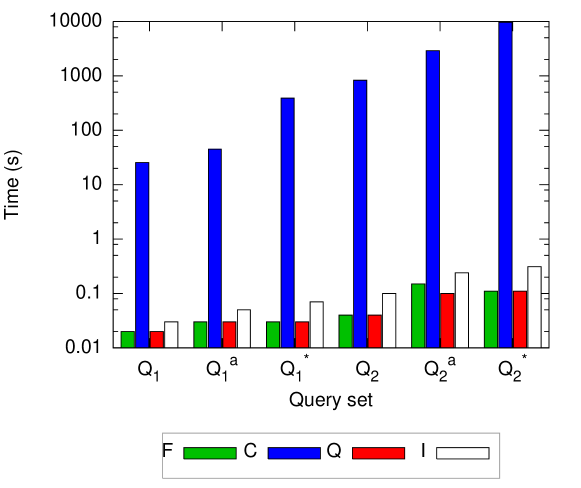
Figure 6 shows the end-to-end running time of the different methods. This demonstrates clearly the dramatically slow running time of the clustering method: reaching several hours to operate on a single, moderate-sized dataset. As the dimensionality increases, this becomes exponentially worse. By contrast, the time needed by the other strategies is negligible: always less than a second, and typically less than a tenth of a second. The optimization and consistency steps take essentially no time at all, compared to the data handling and processing. On the other hand, all methods have virtually constant time as a function of the number of tuples in the data.
Returning to the accuracy, over the -way marginals and variations, the approach of materializing the base counts () is not competitive, while the clustering strategy () achieves the least error. The more lightweight Fourier-based approach achieves slightly more error, but is much more scalable. As the degree of the marginals increases (, Figure 5(e), and , Figure 5(f)), the trivial solution of materializing the base cells becomes more accurate. For workloads that are made up of high-degree marginals, this method dominates the other approaches, although such workloads are considered less realistic.
6 Concluding Remarks
We considered the problem of releasing data based on linear queries, which captures the common case of data cubes and marginals. We showed how existing matrix-based strategies can be improved by using non-uniform noise based on the query workload. Our results show that such non-uniform noise results in significantly lower error across all cases considered. Further, the cost of this is low, and the results can be made consistent with minimal extra effort.
Other notions of consistency are possible within this framework. For example, it is sometimes required that the query answers correspond to a data set in which all counts are integral and non-negative. This can be achieved when the method actually materializes a noisy set of base counts (as in the case of strategy ) by adding the constraints that and rounding the results to the nearest integer. It remains to show how to enforce such consistency constraints efficiently when base counts are not explicitly materialized.
On the theoretical side, we have shown bounds on accurate -way release under differential privacy of . An open problem is to close the gap between this and the lower bound of .
Acknowledgments. We thank Adam D. Smith and Moritz Hardt for multiple useful comments and suggestions.
References
- [1] B. Barak, K. Chaudhuri, C. Dwork, S. Kale, F. McSherry, and K. Talwar. Privacy, accuracy, and consistency too: a holistic solution to contingency table release. In PODS, 2007.
- [2] A. Blum, K. Ligett, and A. Roth. A learning theory approach to non-interactive database privacy. In STOC, 2008.
- [3] T.-H. H. Chan, E. Shi, and D. Song. Private and continual release of statistics. In ICALP, 2010.
- [4] G. Cormode, C. Procopiuc, E. Shen, D. Srivastava, and T. Yu. Differentially private spatial decompositions. In ICDE, 2012.
- [5] G. Cormode, C. Procopiuc, D. Srivastava, and T. Tran. Differentially private publication of sparse data. In ICDT, 2012.
- [6] B. Ding, M. Winslett, J. Han, and Z. Li. Differentially private data cubes: optimizing noise sources and consistency. In SIGMOD, 2011.
- [7] C. Dwork. Differential privacy. In ICALP, 2006.
- [8] C. Dwork, K. Kenthapadi, F. McSherry, I. Mironov, and M. Naor. Our data, ourselves: Privacy via distributed noise generation. In EUROCRYPT, 2006.
- [9] C. Dwork, F. McSherry, K. Nissim, and A. Smith. Calibrating noise to sensitivity in private data analysis. In Theory of Cryptography, 2006.
- [10] A. Gupta, A. Roth, and J. Ullman. Iterative constructions and private data release. CoRR, abs/1107.3731, 2011.
- [11] M. Hardt, K. Ligett, and F. McSherry. A simple and practical algorithm for differentially private data release. CoRR, abs/1012.4763, 2010.
- [12] M. Hardt and G. N. Rothblum. A multiplicative weights mechanism for privacy-preserving data analysis. In FOCS, 2010
- [13] M. Hardt and K. Talwar. On the geometry of differential privacy. In STOC, 2010.
- [14] M. Hay, V. Rastogi, G. Miklau, and D. Suciu. Boosting the accuracy of differentially-private histograms through consistency. In VLDB, 2010.
- [15] S. P. Kasiviswanathan, M. Rudelson, A. Smith, and J. Ullman. The price of privately releasing contingency tables and the spectra of random matrices with correlated rows. In STOC, 2010.
- [16] C. Li, M. Hay, V. Rastogi, G. Miklau, and A. McGregor. Optimizing linear counting queries under differential privacy. In PODS, 2010.
- [17] C. Li and G. Miklau. Efficient batch query answering under differential privacy. CoRR, abs/1103.1367, 2011.
- [18] Y. Li, Z. Zhang, M. Winslett, and Y. Yang. Compressive mechanism: Utilizing sparse representation in differential privacy. In WPES, 2011.
- [19] F. McSherry and I. Mironov. Differentially private recommender systems: Building privacy into the netflix prize contenders. In KDD, 2009.
- [20] C. R. Rao. Linear statistical inference and its applications. Wiley, 1965.
- [21] S. Boyd and L. Vandenberghe. Convex Optimization. Cambridge Univ. Press, 2004.
- [22] A. Roth and T. Roughgarden. Interactive privacy via the median mechanism. In STOC, 2010.
- [23] X. Xiao, G. Wang, and J. Gehrke. Differential privacy via wavelet transforms. In ICDE, 2010.
Appendix A Budgeting for -differential privacy
Proof of Proposition 3.1, part (ii).
Consider a matrix with entries , where . Because -norm of any column of is at most by Theorem 2.2 adding to values Gaussian noise with variance guarantees -differential privacy. Given these noisy values which we denote as , the noisy values can be computed as and so has variance , which is at most for as desired. ∎
Proof of Corollary 3.3 for -differential privacy.
For -differential privacy the analog of optimization problem (4) – (6) is:
We can ignore the multiplicative factor in the objective function, because it doesn’t change the optimum solution. Then the corresponding Lagrange function is:
Using condition we have:
so and we have
which gives and . The value of the objective function is now given as:
If all values are equal to this gives . ∎
Appendix B Fourier strategy–Uniform Noise
In this section, we provide a tighter analysis of the expected noise that results from using the Fourier strategy with uniform noise. This is to be compared with the bound of stated in [1, Theorem 7].
Theorem B.1.
Let the query workload consist of marginals and be the set of Fourier coefficients, corresponding to this workload, such that . Then if we release all Fourier coefficients in via the Laplace mechanism with uniform noise and use them to compute private values of the marginals for each marginal bounds on the noise per marginal can be given as:
-
1.
-
2.
with probability at least
Proof.
Let and w.l.o.g, assume that , so:
| (8) |
The last step follows due to the symmetry of the Laplace random variables . Note that for iid unbiased random variables , , using Jensen’s inequality. Hence, using the linearity of expectation and the fact that , we have:
| (9) |
To get a concentration bound for the second part of the Theorem, we use the fact that with probability at least , (see, e.g. [3]).
Substituting this in (8), we have with probability ,
Rescaling by a factor of means that by a union bound this holds for all . ∎
Appendix C Omitted Proofs
Proof of Lemma 4.2.
We have , and . For the set of all -way marginals the matrices , and have the following entries:
where we abuse notation indexing entries by vectors only if entries corresponding to respective subsets exist. Here, indexes marginals. Formally, we use all pairs , where and to index over . We use an index , where to index over and a regular index to index over . The grouping number of is equal to because the groups consist of individual rows of , so for all we have and . Using and substituting entries of , we have , where we use index as described above. Thus,
Now, using Corrollary 3.3 privacy (and assuming ) we get the sum of the noise variances over all entries equal to
Thus, dividing by , the variance of noise per entry of a marginal table is . By Jensen’s inequality, the expected magnitude of noise per entry is .
For -differential privacy Corollary 3.3 gives variance at most:
which gives expected noise per marginal entry. ∎