The behaviour of constrained caloric curves as ultimate signature of a phase transition for hot nuclei

Abstract

Simulations based on experimental data obtained from multifragmenting quasi-fused nuclei produced in central ¹²⁹Xe + ^natSn collisions have been used to deduce event by event freeze-out properties on the thermal excitation energy range 4-12 AMeV. From these properties and temperatures deduced from proton transverse momentum fluctuations constrained caloric curves have been built. At constant average volumes caloric curves exhibit a monotonous behaviour whereas for constrained pressures a backbending is observed. Such results support the existence of a first order phase transition for hot nuclei.

1 Introduction

One of the most important challenges of heavy-ion collisions at intermediate energies is the identification and characterization of the nuclear liquid-gas phase transition for hot nuclei, which was earlier theoretically predicted for nuclear matter [1]. In the last fifteen years a big effort to accumulate experimental indications of the phase transition has been made. Statistical mechanics for finite systems appeared as a key issue to progress by proposing new first-order phase transition signatures related to thermodynamic anomalies like negative microcanonical heat capacity and bimodality of an order parameter [2, 3, 4]. Correlated temperature and excitation energy measurements, commonly termed caloric curves, were the first studied possible signatures of phase transition. However in spite of the observation of a plateau in some caloric curves, no decisive conclusion could be extracted [1, 5, 6, 7]. The reason is that experimentally it is not possible to explore the caloric curves at constant pressure or constant average volume, which is required for an unambiguous phase transition signature. Indeed, theoretical studies show that if many different caloric curves can be generated depending on the path followed in the thermodynamical landscape, constrained caloric curves exhibit different behaviours in presence of a first order phase transition: a monotonous evolution at constant average volume and a back bending of curves at constrained pressures [8, 9]. With the help of a simulation able to correctly reproduce most of the experimental observables measured for hot nuclei formed in central collisions (quasi-fused systems, QF, from ${}^{129}Xe$+${}^{nat}Sn$, 32-50 AMeV), event by event properties at freeze-out were restored and used to build constrained caloric curves. The definition of pressure in the microcanonical ensemble is presented in section 2. Then, in section 3, simulations to recover freeze-out properties of multifragmentation events [10, 11] are briefly described and constrained caloric curves deduced are discussed. Section 4 is dedicated to the description of the thermometer finally chosen and to comparisons of results relative to a caloric curve without any constraints. Constrained caloric curves with temperatures including quantum fluctuations are presented in section 5. Section 6 is devoted to a discussion of the various results. Conclusions are given in section 7.

2 Pressure in the microcanonical ensemble

Let us consider a gas of weakly interacting fragments (i.e. they interact only by Coulomb and excluded volume), which corresponds to the freeze-out configuration. Within a microcanonical ensemble, the statistical width of a configuration $C$, defined by the mass, charge and internal excitation energy of each of the constituting $M_{C}$ fragments, writes

$$W_{C}(A,Z,E,V)=\frac{1}{M_{C}!}\chi V^{M_{C}}\prod_{n=1}^{M_{C}}\left(\frac{\rho_{n}(\epsilon_{n})}{h^{3}}(mA_{n})^{3/2}\right)$$

$$~{}\frac{2\pi}{\Gamma(3/2(M_{C}-2))}~{}\frac{1}{\sqrt{({\rm det}I})}~{}\frac{(2\pi K)^{3/2M_{C}-4}}{(mA)^{3/2}},$$ (1)

where $I$ is the moment of inertia, $K$ is the thermal kinetic energy, $V$ is the freeze-out volume and $\chi V^{M_{C}}$ stands for the free volume or, equivalently, accounts for inter-fragment interaction in the hard-core idealization.

The microcanonical equations of state are

$$T=\left(\frac{\partial S}{\partial E}\right)^{-1}|_{V,A},$$

$$P/T=\left(\frac{\partial S}{\partial V}\right)|_{E,A},$$

$$-\mu/T=\left(\frac{\partial S}{\partial A}\right)|_{E,V}.$$ (2)

Taking now into account that $S=\ln Z=\ln\sum_{C}W_{C}$ and that $\partial W_{C}/\partial V=\left(M_{C}/V\right)W_{C}$, it comes out that

$$P/T=\left(\frac{\partial S}{\partial V}\right) = \frac{1}{\sum_{C}W_{C}}\sum_{C}\frac{\partial W_{C}}{\partial V}$$ (3)

$$= \frac{1}{V}\frac{\sum_{C}M_{C}W_{C}}{\sum_{C}W_{C}}=\frac{<M_{C}>}{V}.$$

The microcanonical temperature is also easily deduced from its statistical definition [12]:

$$T=\left(\frac{\partial S}{\partial E}\right)^{-1} = (\frac{1}{\sum_{C}W_{C}}\sum_{C}W_{C}(3/2M_{C}-5/2)/K)^{-1}$$ (4)

$$= <(3/2M_{C}-5/2)/K>^{-1}.$$

where $K$ is the total thermal kinetic energy of the system at freeze-out.

As $M_{C}$, the total multiplicity at freeze-out, is large, the pressure $P$ can be well approximated by

$$P=\frac{2}{3}\frac{<K>}{V}.$$

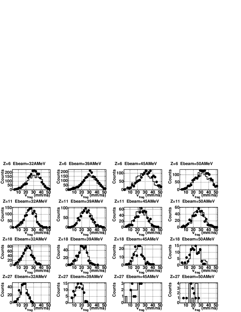
Figure 1: Comparison between the experimental velocity spectra (full points) of fragments of a given charge and the simulated ones (histograms). Each row refers to a different fragment charge: starting from the top Z=6, Z=11, Z=18 and Z=27. Each column refers to a different beam energy: starting from the left 32, 39, 45 and 50 AMeV. From [11].

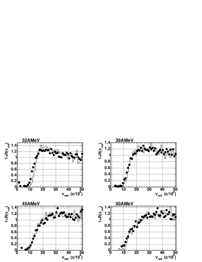
Figure 2: Comparison betwwen the experimental (full points) and simulated (histograms) reduced relative velocity correlation functions for fragments. Each panel refers to a different beam energy. From [11].

3 Event by event freeze-out properties

Starting from all the available asymptotic experimental information (charged particle energy spectra, average and standard deviation of fragment velocity spectra and calorimetry) of selected QF sources produced in central ¹²⁹Xe+^natSn collisions which undergo multifragmentation, a simulation was performed to reconstruct freeze-out properties event by event [10, 11]. The method requires data with a very high degree of completeness (total detected charge $\geq$93% of the total charge of the system), which is crucial for a good estimate of Coulomb energy. QF sources are reconstructed, event by event, in the reaction centre of mass, from all the fragments and twice the charged particles emitted in the range $60-120^{\circ}$ in order to exclude a major part of pre-equilibrium emission. Dressed excited fragments and particles at freeze-out are described by spheres at normal density. Then the excited fragments subsequently deexcite while flying away. Four free parameters are used to recover the data at each incident energy: the percentage of measured particles which were evaporated from primary fragments, the collective radial energy, a minimum distance between the surface of products at freeze-out and a limiting temperature for fragments. The limiting temperature, related to the vanishing of level density for fragments [13], was mandatory to reproduce the observed widths of fragment velocities. Indeed, Coulomb repulsion plus collective energy plus thermal kinetic energy (directed at random) plus spreading due to fragment decays are responsible for about 60-70% of the observed widths. By introducing a limiting temperature for fragments, thermal kinetic increases, due to energy conservation, which produces the missing percentage for the widths of final velocity distributions. The agreement between experimental and simulated velocity/energy spectra for fragments and for the different beam energies is quite remarkable (see figure 1). Relative velocities between fragment pairs were also compared through reduced relative velocity correlation functions [14, 15] (see figure 2). Again a good agreement is obtained between experimental data and simulations, which indicates that the retained method (freeze-out topology built up at random) and parameters are sufficiently relevant to correctly describe the freeze-out configurations, including volumes. Finally one can also note that the agreement between experimental and simulated energy spectra for protons and alpha-particles (see an example in figure 3) is not very good at high energy. This comes from the fact that we have chosen (to limit the number of parameters of the simulation) a single value for the percentage of all measured particles which were evaporated from primary fragments. We shall see in the following section how to correct for temperature measurements derived from protons.

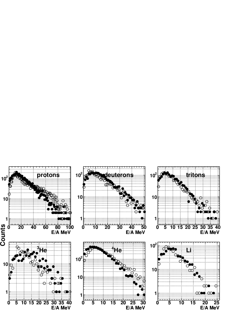
Figure 3: Centre of mass energy spectra for protons, deuterons, tritons, ³He, ⁴He and ⁷Li for the reaction at 39 AMeV. Open points are the simulated data, while full points are the experimental ones. From [11].

From the simulations it is then possible to recover, event by event, the different quantities needed to build constrained caloric curves, namely the thermal excitation energy of QF hot nuclei, $E^{*}$ (total excitation minus collective energy) with an estimated systematic error of around 1 AMeV, the kinetic temperature $T_{kin}$ at freeze-out, the freeze-out volume $V$ (see envelopes of figure 8 from [11]) and the total thermal kinetic energy at freeze-out $K$. In simulations, Maxwell-Boltzmann distributions are used to reproduce the thermal kinetic properties at freeze-out and consequently the deduced temperatures, $T_{kin}$, are classical.

Constrained caloric curves, which correspond to correlated values of $E^{*}$ and $T_{kin}$ have been derived for QF hot nuclei with Z restricted to the range 80-100, which corresponds to the A domain 194-238, in order to reduce any possible effect of mass variation on caloric curves [7] (see figure 4). Curves for internal fragment temperatures are also shown in the figure. For different average freeze-out volumes expressed as a function of $V_{0}$, the volume of the QF nuclei at normal density, a monotonous behaviour of caloric curves is observed as theoretically expected. The caloric curves when pressure has been constrained exhibit a backbending and moreover the qualitative evolution of curves with increasing pressure exactly corresponds to what is theoretically predicted with a microcanonical lattice gas model [8]. However by extrapolating at higher pressures, one could infer a critical temperature around 20 MeV. Such a value is within the range calculated for infinite nuclear matter whereas a lower value is expected for nuclei in relation with surface and Coulomb effects [1]. At that point, one may wonder if $T_{kin}$ is a relevant thermometer. We shall see, in what follows, that the final choice was to use, for protons thermally emitted at freeze-out, a new thermometer recently proposed for which quantum effects can be included.

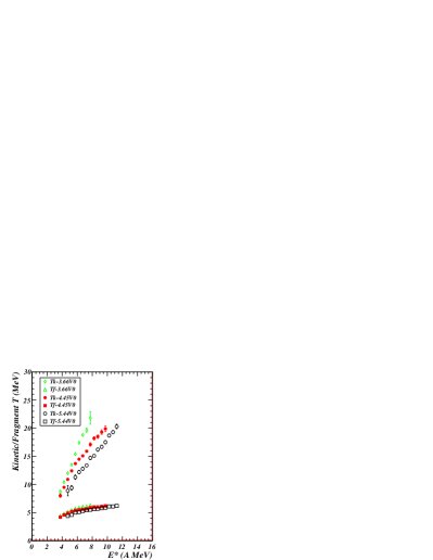
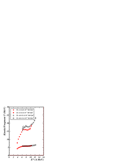
Figure 4: Caloric curves (kinetic temperature versus thermal excitation energy) constrained at average volumes (left) and for selected ranges of pressure (right) and the corresponding internal temperatures for fragments. Error bars correspond to statistical errors. From [16].

4 Temperatures from proton transverse momentum fluctuations

Very recently a new method for measuring the temperature of hot nuclei was proposed [17, 18]. It is based on momentum fluctuations of emitted particles like protons in the centre of mass frame of the fragmenting nuclei. On the classical side, assuming a Maxwell-Boltzmann distribution of the momentum yields, the temperature T is deduced from the quadrupole momentum fluctuations defined in a direction transverse to the beam axis:
$\sigma^{2}$ = $<Q_{xy}^{2}>$ - $<Q_{xy}>^{2}$ = $4m^{2}T^{2}$
with $Q_{xy}$ = $P_{x}^{2}$ - $P_{y}^{2}$; m and P are the mass and linear momentum of emitted particles. Taking into account the quantum nature of particles, a correction $F_{QC}$ related to a Fermi-Dirac distribution was also proposed [18, 19].
In that case $\sigma^{2}$ = $4m^{2}T^{2}$ $F_{QC}$ where $F_{QC}$ = $0.2(T/\epsilon_{f})^{-1.71}$ + 1;
$\epsilon_{f}$ = 36 $(\rho/\rho_{0})^{2/3}$ is the Fermi energy of nuclear matter at density $\rho$ and $\rho_{0}$ corresponds to normal density.

Before using the thermometer with protons to build constrained caloric curves, it was important to verify several things. With the classical simulation (freeze-out and asymptotic proton momenta) , it is possible to test the agreement with the proposed classical thermometer. Moreover the effects of secondary decays on temperature measurements can be estimated. Figure 6 shows different caloric curves without constraints. Note that the selection in Z and A of hot nuclei is the same as in the previous section. It was verified that, within statistical error bars, at a given thermal excitation energy transverse momentum fluctation values are the same for our selection or by selecting only a single (A and Z) hot nucleus. Open diamonds refer to classical temperatures calculated from momentum fluctuations for protons thermally emitted at freeze-out. Within the statistical error bars they perfectly superimposed on $T_{kin}$ values (see figure 2 of [16]), which just verifies that Maxwell-Boltzmann distribution was correctly implemented in the simulation. Full squares correspond to classical temperatures calculated from momentum fluctuations for protons after the secondary decay stage. We note that the caloric curve is distorted, which means that it is not possible to use experimental data from protons to measure temperatures. Moreover, in this case, quantum corrections for temperatures can not be made because protons are emitted at different stages of deexcitation with different Fermi energy values. In figure 6 classical temperatures calculated from experimental proton data are also shown (full points). As for temperatures calculated from asymptotic proton data of simulations, a monotonous behaviour of the caloric curve is observed. One also note the differences between the two sets of temperature values, which are related to the fact that, as indicated in the previous section, simulations do not describe experimental proton energy spectra very well. Those temperature differences will be used to correct classical temperatures derived from simulated protons at freeze-out.

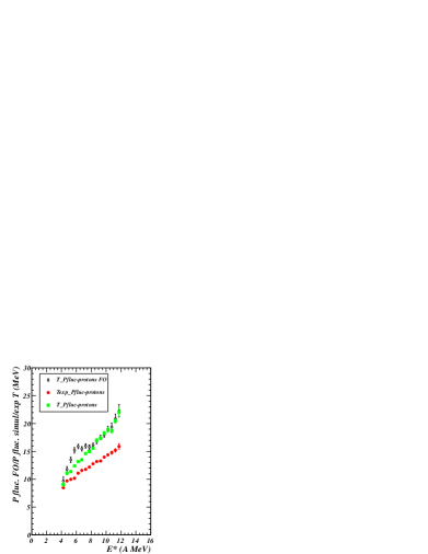
Figure 5: Caloric curves (classical temperature from proton transverse momentum fluctuations versus thermal excitation energy) for protons (simulation) thermally emitted at freeze-out (open diamonds), for protons (simulation) after the secondary decay stage (full squares), and from protons experimentally measured (full points). Error bars correspond to statistical errors

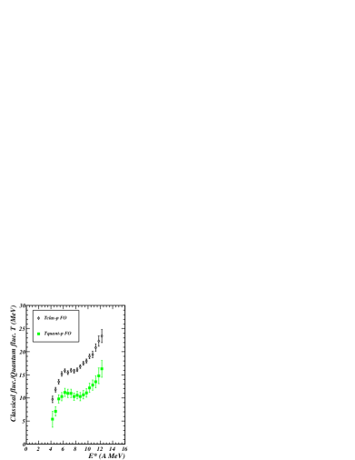
Figure 6: Caloric curves: classical temperature (open diamonds)/ quantum corrected temperature (full squares) from proton transverse momentum fluctuations versus thermal excitation energy. Protons (simulation) are thermally emitted at freeze-out. Error bars include statistical and systematic errors.

It finally appears that the only way to extract temperatures from proton transverse momentum fluctuations taking into account quantum effects is to use protons thermally emitted at freeze-out. In that case classical temperature values from simulations must be extracted and corrected and then, quantum corrections applied, which needs Fermi energy values. Those values can be estimated from semi-classical calculations (Xn+Sn at 32 AMeV and Sn+Sn at 50 AMeV) [20, 21]: protons thermally emitted at freeze-out at time around 100-120 fm/c after the beginning of collisions come from a low density uniform source. For the two incident energies low densities around $\rho\sim 0.4\rho_{0}$ are calculated which corresponds to $\epsilon_{f}\sim$ 20 MeV. We have introduced a systematic error of $\pm$ 0.1$\rho_{0}$ for the calculation of $\epsilon_{f}$ and consequently a systematic error for “quantum” temperatures of $\pm$ 0.6-0.5 MeV on the considered thermal excitation energy range. Figure 6 shows the final caloric curve with temperatures from quantum fluctuations (full squares). It exhibits a plateau around a temperature of 10-11 MeV on the $E^{*}$ range 5-10 AMeV. For comparison the caloric curve with classical temperatures derived from the simulation is also shown (open diamonds).

5 Constrained caloric curves with quantum temperatures

Constrained caloric curves, which correspond to correlated values of $E^{*}$ and quantum corrected temperatures have been determined. Accordingly $E^{*}$ values, which were initially derived from experimental calorimetry including estimated correction for neutrons (see [10]), have been corrected a posteriori using quantum temperatures at freeze-out. Pressure values were also corrected using quantum temperatures. In figure 7 (left) we have constructed caloric curves for two different average freeze-out volumes corresponding to the ranges 3.0-4.0$V_{0}$ and 5.0-6.0$V_{0}$ where $V_{0}$ correspond to the volume of the QF nuclei at normal density. Again as theoretically expected a monotonous behaviour of caloric curves is observed. Figure 7 (right) shows the caloric curves when pressure has been constrained within two domains: 1.3-4.5 and 4.5-7.9 $10^{-2}$ MeVfm^-3. Backbending are clearly seen especially for the lower pressure range. For higher pressures the backbending of the caloric curve is largely reduced and one can estimate that the critical temperature is around 12-13 MeV for the selected hot nuclei.

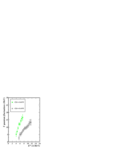
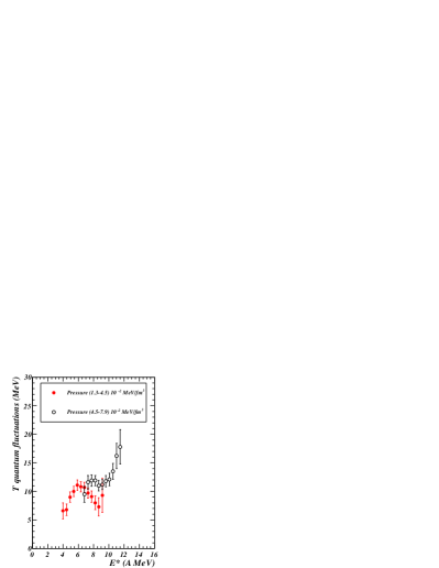
Figure 7: Caloric curves (quantum corrected temperature versus thermal excitation energy) constrained at average volumes (left) and for selected ranges of pressure (right). Error bars include statistical and systematic errors.

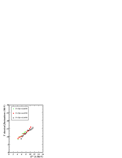
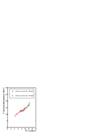
Figure 8: Caloric curves (classical temperature derived from experimental proton data versus thermal excitation energy) constrained at average volumes (left) and for selected ranges of pressure (right). Error bars correspond to statistical errors.

6 Discussion

First of all, as far as internal temperature for fragments are concerned (see figure 4), one can observe that they perfectly agree, for our A range, with those calculated with the well known “He/Li thermometer” used in [5, 7] keeping the proposed prefactor 16. Note that similar temperature values are also obtained from our data (see figure 2 from [16]). This is a strong indication that the He/Li thermometer mainly reflects the internal temperature of fragments in relation with the strong secondary emission of alpha-particles and Li isotopes. As indicated in [7] those plateau temperatures can be interpreted as representing the limiting temperatures resulting from Coulomb instabilities of heated nuclei which has long been predicted [22]. Indeed, for thermally equilibrated QF hot nuclei one expects internal temperature for fragments equal to the limiting temperature of the fragmenting system. As a direct consequence internal fragment temperatures must reflect the evolution of limiting temperature with A of hot nuclei, which is indeed experimentally observed [7].

For a finite piece of nuclear matter like a hot nucleus the microcanonical ensemble is the most relevant ensemble and the kinetic/microcanonical temperature is the relevant parameter to build caloric curves and deduce information on a possible phase transition. On the other hand, one may also recall that dispersions in fragment transverse momentum spectra generated in projectile fragmentation were succesfully explained by adding the Fermi momenta of individual nucleons in fragments [23], which is a consequence of the quantum nature of nucleons. For multifragmentation reactions a similar approach was first proposed in [24] to qualitatively explain the different temperatures obtained from various observables (kinetic energies, level populations, isotope ratios). Thus, the use of the thermometer recently proposed based on quantum fluctuations [18] was a good opportunity to better investigate the behaviour of caloric curves especially under constraints in volume and pressure. The behaviour predicted by theoretical works for a first order phase transition is observed and confirms results obtained for other signals: negative microcanonical heat capacity and bimodality of an order parameter.

The last point that we want to discuss concerns information which can be directly deduced from experimental data like proton transverse momentum fluctuations. In that case as previously indicated Fermi energies can not be estimated and only classical temperatures can be calculated. From simulations we have seen previously that secondary decays distorted caloric curves. Results displayed in figure 8 fully confirm this observation: constrained caloric curves built with classical temperatures derived from experimental proton momenta also exhibit a monotonous behaviour and do not show any dependence upon average volumes or pressures, which prevent any direct information.

7 Conclusions

Several caloric curves have been derived for hot nuclei from quasi-fused systems using a new thermometer based on proton transverse momentum fluctuations including quantum effects. The unconstrained caloric curve exhibits a plateau at a temperature of around 10-11 MeV on the thermal excitation energy range 5-10 AMeV. For constrained caloric curves (volume and pressure) we observe what is expected for a first order phase transition for finite systems in the microcanonical ensemble, namely a monotonous behaviour at constant average volumes and backbending for constrained pressures. After the observation of negative microcanonical heat capacity and bimodality the behaviour of caloric curves is the ultimate signature of a first order phase transition for hot nuclei.

The exit, at high excitation, of the spinodal region and of the coexistence region around respectively 8 and 10 AMeV are in good agreement (within error bars) with spinodal [25] and bimodality [4] signals. Note also that 10 AMeV corresponds to first experimental indications for the onset of vaporization [26, 27, 28, 29].

Finally, one can infer from the present studies that the temperatures obtained with the He/Li thermometer, which was largely used in the past, seem mainly reflect the internal temperatures of fragments in the excitation energy range 5-10 AMeV.

The authors are indebted to A. Bonasera for private information and discussions.é

References

References

- [1] Borderie B 2002 J. Phys. G: Nucl. Part. Phys. 28 R217
- [2] Chomaz P, Gulminelli F et al (eds) 2006 Dynamics and Thermodynamics with Nuclear Degrees of Freedom vol 30 of Eur. Phys. J. A (Berlin Heidelberg: Springer-Verlag)
- [3] Borderie B and Rivet M F 2008 Prog. Part. Nucl. Phys. 61 551
- [4] Bonnet E, Mercier D et al (INDRA Collaboration) 2009 Phys. Rev. Lett. 103 072701
- [5] Pochodzalla J, M hlenkamp T et al (ALADIN Collaboration) 1995 Phys. Rev. Lett. 75 1040
- [6] Ma Y G, Siwek A et al (INDRA Collaboration) 1997 Phys. Lett. B 390 41
- [7] Natowitz J B, Wada R et al 2002 Phys. Rev. C 65 034618
- [8] Chomaz P, Duflot V and Gulminelli F 2000 Phys. Rev. Lett. 85 3587
- [9] Furuta T and Ono A 2006 Phys. Rev. C 74 014612
- [10] Piantelli S, Le Neindre N et al (INDRA Collaboration) 2005 Phys. Lett. B 627 18
- [11] Piantelli S, Borderie B et al (INDRA Collaboration) 2008 Nucl. Phys. A 809 111
- [12] Raduta A H and Raduta A R, 2002 Nucl. Phys. A 703 876
- [13] Koonin S E and Randrup J, 1987 Nucl. Phys. A 474 173
- [14] Kim Y D, de Souza R T et al 1992 Phys. Rev. C 45 338
- [15] Tăbăcaru G, Rivet M F et al (INDRA Collaboration) 2006 Nucl. Phys. A 764 371
- [16] Borderie B, Piantelli S et al (INDRA Collaboration) 2012 Proc. Int. Workshop on Multifragmentaton and related topics (Caen) http://dx.doi.org/10.1051/epjconf/20123100005
- [17] Wuenschel S, Bonasera A et al 2010 Nucl. Phys. A 843 1
- [18] Zheng H and Bonasera A 2011 Phys. Lett. B 696 178
- [19] Zheng H and Bonasera A 2011 (Preprint nucl-th/1112.4098v1)
- [20] Frankland J D, Borderie B et al (INDRA Collaboration) 2001 Nucl. Phys. A 689 940
- [21] Rizzo J, Colonna M et al 2007 Phys. Rev. C 76 024611
- [22] Levit S, Bonche P 1985 Nucl. Phys. A 437 426
- [23] Goldhaber A S 1974 Phys. Lett. B 53 306
- [24] Bauer W 1995 Phys. Rev. C 51 803
- [25] Tăbăcaru G, Borderie B et al 2003 Eur. Phys. J A 18 103
- [26] Tsang M B, Hsi W C et al 1993 Phys. Rev. Lett. 71 1502
- [27] Borderie B, Durand D et al 1996 Phys. Lett. B 388 224
- [28] Borderie B, Gulminelli F et al 1999 Eur. Phys. J A 6 197
- [29] Pinkowski L, Bohne W et al 2000 Phys. Lett. B 472 15