Equivalence of distance-based and RKHS-based statistics in hypothesis testing

Abstract

We provide a unifying framework linking two classes of statistics used in two-sample and independence testing: on the one hand, the energy distances and distance covariances from the statistics literature; on the other, maximum mean discrepancies (MMD), that is, distances between embeddings of distributions to reproducing kernel Hilbert spaces (RKHS), as established in machine learning. In the case where the energy distance is computed with a semimetric of negative type, a positive definite kernel, termed distance kernel, may be defined such that the MMD corresponds exactly to the energy distance. Conversely, for any positive definite kernel, we can interpret the MMD as energy distance with respect to some negative-type semimetric. This equivalence readily extends to distance covariance using kernels on the product space. We determine the class of probability distributions for which the test statistics are consistent against all alternatives. Finally, we investigate the performance of the family of distance kernels in two-sample and independence tests: we show in particular that the energy distance most commonly employed in statistics is just one member of a parametric family of kernels, and that other choices from this family can yield more powerful tests.

, , and

1 Introduction

The problem of testing statistical hypotheses in high dimensional spaces is particularly challenging, and has been a recent focus of considerable work in both the statistics and the machine learning communities. On the statistical side, two-sample testing in Euclidean spaces (of whether two independent samples are from the same distribution, or from different distributions) can be accomplished using a so-called energy distance as a statistic [Székely and Rizzo (2004, 2005), Baringhaus and Franz (2004)]. Such tests are consistent against all alternatives as long as the random variables have finite first moments. A related dependence measure between vectors of high dimension is the distance covariance [Székely, Rizzo and Bakirov (2007), Székely and Rizzo (2009)], and the resulting test is again consistent for variables with bounded first moment. The distance covariance has had a major impact in the statistics community, with Székely and Rizzo (2009) being accompanied by an editorial introduction and discussion. A particular advantage of energy distance-based statistics is their compact representation in terms of certain expectations of pairwise Euclidean distances, which leads to straightforward empirical estimates. As a follow-up work, Lyons (2013) generalized the notion of distance covariance to metric spaces of negative type (of which Euclidean spaces are a special case).

On the machine learning side, two-sample tests have been formulated based on embeddings of probability distributions into reproducing kernel Hilbert spaces [Gretton et al. (2007, 2012a)], using as the test statistic the difference between these embeddings: this statistic is called the maximum mean discrepancy (MMD). This distance measure was also applied to the problem of testing for independence, with the associated test statistic being the Hilbert–Schmidt independence criterion (HSIC) [Gretton et al. (2005, 2008), Smola et al. (2007), Zhang et al. (2011)]. Both tests are shown to be consistent against all alternatives when a characteristic RKHS is used [Fukumizu et al. (2009), Sriperumbudur et al. (2010)].

Despite their striking similarity, the link between energy distance-based tests and kernel-based tests has been an open question. In the discussion of [Székely and Rizzo (2009), Gretton, Fukumizu and Sriperumbudur (2009), page 1289] first explored this link in the context of independence testing, and found that interpreting the distance-based independence statistic as a kernel statistic is not straightforward, since Bochner’s theorem does not apply to the choice of weight function used in the definition of the distance covariance (we briefly review this argument in Section 5.3). Székely and Rizzo (2009), Rejoinder, page 1303, confirmed that the link between RKHS-based dependence measures and the distance covariance remained to be established, because the weight function is not integrable. Our contribution resolves this question, and shows that RKHS-based dependence measures are precisely the formal extensions of the distance covariance, where the problem of nonintegrability of weight functions is circumvented by using translation-variant kernels, that is, distance-induced kernels, introduced in Section 4.1.

In the case of two-sample testing, we demonstrate that energy distances are in fact maximum mean discrepancies arising from the same family of distance-induced kernels. A number of interesting consequences arise from this insight: first, as the energy distance (and distance covariance) derives from a particular choice of a kernel, we can consider analogous quantities arising from other kernels, and yielding more sensitive tests. Second, in relation to Lyons (2013), we obtain a new family of characteristic kernels arising from general semimetric spaces of negative type, which are quite unlike the characteristic kernels defined via Bochner’s theorem [Sriperumbudur et al. (2010)]. Third, results from [Gretton et al. (2009), Zhang et al. (2011)] may be applied to obtain consistent two-sample and independence tests for the energy distance, without using bootstrap, which perform much better than the upper bound proposed by Székely, Rizzo and Bakirov (2007) as an alternative to the bootstrap.

In addition to the energy distance and maximum mean discrepancy, there are other well-known discrepancy measures between two probability distributions, such as the Kullback–Leibler divergence, Hellinger distance and total variation distance, which belong to the class of $f$-divergences. Another popular family of distance measures on probabilities is the integral probability metric [Müller (1997)], examples of which include the Wasserstein distance, Dudley metric and Fortet–Mourier metric. Sriperumbudur et al. (2012) showed that MMD is an integral probability metric and so is energy distance, owing to the equality (between energy distance and MMD) that we establish in this paper. On the other hand, Sriperumbudur et al. (2012) also showed that MMD (and therefore the energy distance) is not an $f$-divergence, by establishing the total variation distance as the only discrepancy measure that is both an IPM and $f$-divergence.

The equivalence established in this paper has two major implications for practitioners using the energy distance or distance covariance as test statistics. First, it shows that these quantities are members of a much broader class of statistics, and that by choosing an alternative semimetric/kernel to define a statistic from this larger family, one may obtain a more sensitive test than by using distances alone. Second, it shows that the principles of energy distance and distance covariance are readily generalized to random variables that take values in general topological spaces. Indeed, kernel tests are readily applied to structured and non-Euclidean domains, such as text strings, graphs and groups [Fukumizu et al. (2009)].

The structure of the paper is as follows: in Section 2, we introduce semimetrics of negative type, and extend the notions of energy distance and distance covariance to semimetric spaces of negative type. In Section 3, we provide the necessary definitions from RKHS theory and give a review of the maximum mean discrepancy (MMD) and the Hilbert–Schmidt independence criterion (HSIC), the RKHS-based statistics used for two-sample and independence testing, respectively. In Section 4, the correspondence between positive definite kernels and semimetrics of negative type is developed, and it is applied in Section 5 to show the equivalence between a (generalized) energy distance and MMD (Section 5.1), as well as between a (generalized) distance covariance and HSIC (Section 5.2). We give conditions for these quantities to distinguish between probability measures in Section 6, thus obtaining a new family of characteristic kernels. Empirical estimates of these quantities and associated two-sample and independence tests are described in Section 7. Finally, in Section 8, we investigate the performance of the test statistics on a variety of testing problems.

This paper extends the conference publication [Sejdinovic et al. (2012)], and gives a detailed technical discussion and proofs which were omitted in that work.

2 Distance-based approach

This section reviews the distance-based approach to two-sample and independence testing, in its general form. The generalized energy distance and distance covariance are defined.

2.1 Semimetrics of negative type

We will work with the notion of a semimetric of negative type on a nonempty set $\mathcal{Z}$, where the “distance” function need not satisfy the triangle inequality. Note that this notion of semimetric is different to that which arises from the seminorm (also called the pseudonorm), where the distance between two distinct points can be zero.

Definition 1 ((Semimetric)).

Let $\mathcal{Z}$ be a nonempty set and let $\rho\dvtx\mathcal{Z}\times\mathcal{Z}\to[0,\infty)$ be a function such that $\forall z,z^{\prime}\in\mathcal{Z}$, [1.]

$\rho(z,z^{\prime})=0$ if and only if $z=z^{\prime}$, and

$\rho(z,z^{\prime})=\rho(z^{\prime},z)$.

Then $(\mathcal{Z},\rho)$ is said to be a semimetric space and $\rho$ is called a semimetric on $\mathcal{Z}$.

Definition 2 ((Negative type)).

The semimetric space $(\mathcal{Z},\rho)$ is said to have negative type if $\forall n\geq 2$, $z_{1},\ldots,z_{n}\in\mathcal{Z}$, and $\alpha_{1},\ldots,\alpha_{n}\in\mathbb{R}$, with$\sum_{i=1}^{n}\alpha_{i}=0$,

$$\sum_{i=1}^{n}\sum_{j=1}^{n}\alpha_{i}\alpha_{j}\rho(z_{i},z_{j})\leq 0.$$ (1)

Note that in the terminology of Berg, Christensen and Ressel (1984), $\rho$ satisfying (1) is said to be a negative definite function. The following proposition is derived from Berg, Christensen and Ressel (1984), Corollary 2.10, page 78, and Proposition 3.2, page 82.

Proposition 3.

[1.]

If $\rho$ satisfies (1), then so does $\rho^{q}$, for $0<q<1$.

$\rho$ is a semimetric of negative type if and only if there exists a Hilbert space $\mathcal{H}$ and an injective map $\varphi\dvtx\mathcal{Z}\to\mathcal{H}$, such that

$$\rho\bigl{(}z,z^{\prime}\bigr{)}=\bigl{\|}\varphi(z)-\varphi\bigl{(}z^{\prime}\bigr{)}\bigr{\|}_{\mathcal{H}}^{2}.$$ (2)

The second part of the proposition shows that $(\mathbb{R}^{d},\|\cdot-\cdot\|^{2})$ is of negative type, and by taking $q=1/2$ in the first part, we conclude that all Euclidean spaces are of negative type. In addition, whenever $\rho$ is a semimetric of negative type, $\rho^{1/2}$ is a metric of negative type, that is, even though $\rho$ may not satisfy the triangle inequality, its square root must do if it obeys (1).

2.2 Energy distance

Unless stated otherwise, we will assume that $\mathcal{Z}$ is any topological space on which Borel measures can be defined. We will denote by $\mathcal{M}(\mathcal{Z})$ the set of all finite signed Borel measures on $\mathcal{Z}$, and by $\mathcal{M}_{+}^{1}(\mathcal{Z})$ the set of all Borel probability measures on $\mathcal{Z}$.

The energy distance was introduced by Székely and Rizzo (2004, 2005) and independently by Baringhaus and Franz (2004) as a measure of statistical distance between two probability measures $P$ and $Q$ on $\mathbb{R}^{d}$ with finite first moments, given by

$$\qquad D_{E}(P,Q)=2\mathbb{E}_{ZW}\|Z-W\|_{2}-\mathbb{E}_{ZZ^{\prime}}\bigl{\|}Z-Z^{\prime}\bigr{\|}_{2}-\mathbb{E}_{WW^{\prime}}\bigl{\|}W-W^{\prime}\bigr{\|}_{2},$$ (3)

where $Z,Z^{\prime}\stackrel{{\scriptstyle\mathrm{i.i.d.}}}{{\sim}}P$ and $W,W^{\prime}\stackrel{{\scriptstyle\mathrm{i.i.d.}}}{{\sim}}Q$. The moment condition is required to ensure that the expectations in (3) is finite. $D_{E}(P,Q)$ is always nonnegative, and is strictly positive if $P\neq Q$. In scalar case, it coincides with twice the Cramér–Von Mises distance.

Following Lyons (2013), the notion can be generalized to a metric space of negative type, which we further extend to semimetrics. Before we proceed, we need to first introduce a moment condition w.r.t. a semimetric $\rho$.

Definition 4.

For $\theta>0$, we say that $\nu\in\mathcal{M}(\mathcal{Z})$ has a finite $\theta$-moment with respect to a semimetric $\rho$ of negative type if there exists $z_{0}\in\mathcal{Z}$, such that $\int\rho^{\theta}(z,z_{0})\,d|\nu|(z)<\infty$. We denote

$$\mathcal{M}_{\rho}^{\theta}(\mathcal{Z})=\biggl{\{}\nu\in\mathcal{M}(\mathcal{Z})\dvtx\exists z_{0}\in\mathcal{Z}\mbox{ s.t. }\int\rho^{\theta}(z,z_{0})\,d|\nu|(z)<\infty\biggr{\}}.$$ (4)

We are now ready to introduce a general energy distance $D_{E,\rho}$.

Definition 5.

Let $(\mathcal{Z},\rho)$ be a semimetric space of negative type, and let $P,Q\in\mathcal{M}_{+}^{1}(\mathcal{Z})\cap\mathcal{M}_{\rho}^{1}(\mathcal{Z})$. The energy distance between $P$ and $Q$, w.r.t. $\rho$ is

$$D_{E,\rho}(P,Q)=2\mathbb{E}_{ZW}\rho(Z,W)-\mathbb{E}_{ZZ^{\prime}}\rho\bigl{(}Z,Z^{\prime}\bigr{)}-\mathbb{E}_{WW^{\prime}}\rho\bigl{(}W,W^{\prime}\bigr{)},$$ (5)

where $Z,Z^{\prime}\stackrel{{\scriptstyle\mathrm{i.i.d.}}}{{\sim}}P$ and $W,W^{\prime}\stackrel{{\scriptstyle\mathrm{i.i.d.}}}{{\sim}}Q$.

If $\rho$ is a metric, as in [Lyons (2013)], the moment condition $P,Q\in\mathcal{M}_{\rho}^{1}(\mathcal{Z})$ is easily seen to be sufficient for the existence of the expectations in (5). Namely, if we take $z_{0},w_{0}\in\mathcal{Z}$ such that $\mathbb{E}_{Z}\rho(Z,z_{0})<\infty$, $\mathbb{E}_{W}\rho(W,w_{0})<\infty$, then the triangle inequality implies:

$$\mathbb{E}_{ZW}\rho(Z,W)\leq\mathbb{E}_{Z}\rho(Z,z_{0})+\mathbb{E}_{W}\rho(W,w_{0})+\rho(z_{0},w_{0})<\infty.$$

If $\rho$ is a general semimetric, however, a different line of reasoning is needed, and we will come back to this condition in Remark 21, where its sufficiency will become clear using the link between positive definite kernels and negative-type semimetrics established in Section 4.

Note that the energy distance can equivalently be represented in the integral form,

$$D_{E,\rho}(P,Q)=-\int\rho\,d\bigl{(}[P-Q]\times[P-Q]\bigr{)},$$ (6)

whereby the negative type of $\rho$ implies the nonnegativity of $D_{E,\rho}$, as discussed by Lyons [(2013), page 10].

2.3 Distance covariance

A related notion to the energy distance is that of distance covariance, which measures dependence between random variables. Let $X$ be a random vector on $\mathbb{R}^{p}$ and $Y$ a random vector on $\mathbb{R}^{q}$. The distance covariance was introduced by Székely, Rizzo and Bakirov (2007), Székely and Rizzo (2009) to address the problem of testing and measuring dependence between $X$ and $Y$ in terms of a weighted $L_{2}$-distance between characteristic functions of the joint distribution of $X$ and $Y$ and the product of their marginals. As a particular choice of weight function is used (we discuss this further in Section 5.3), it can be computed in terms of certain expectations of pairwise Euclidean distances,

$$\mathcal{V}^{2}(X,Y) = \mathbb{E}_{XY}\mathbb{E}_{X^{\prime}Y^{\prime}}\bigl{\|}X-X^{\prime}\bigr{\|}_{2}\bigl{\|}Y-Y^{\prime}\bigr{\|}_{2}$$

$${}+\mathbb{E}_{X}\mathbb{E}_{X^{\prime}}\bigl{\|}X-X^{\prime}\bigr{\|}_{2}\mathbb{E}_{Y}\mathbb{E}_{Y^{\prime}}\bigl{\|}Y-Y^{\prime}\bigr{\|}_{2}$$

$${}-2\mathbb{E}_{XY}\bigl{[}\mathbb{E}_{X^{\prime}}\bigl{\|}X-X^{\prime}\bigr{\|}_{2}\mathbb{E}_{Y^{\prime}}\bigl{\|}Y-Y^{\prime}\bigr{\|}_{2}\bigr{]},$$

where $(X,Y)$ and $(X^{\prime},Y^{\prime})$ are $\stackrel{{\scriptstyle\mathrm{i.i.d.}}}{{\sim}}P_{XY}$. As in the case of the energy distance, Lyons (2013) established that the generalization of the distance covariance is possible to metric spaces of negative type. We extend this notion to semimetric spaces of negative type.

Definition 6.

Let $(\mathcal{X},\rho_{\mathcal{X}})$ and $(\mathcal{Y},\rho_{\mathcal{Y}})$ be semimetric spaces of negative type, and let $X\sim P_{X}\in\mathcal{M}_{\rho_{\mathcal{X}}}^{2}(\mathcal{X})$ and $Y\sim P_{Y}\in\mathcal{M}_{\rho_{\mathcal{Y}}}^{2}(\mathcal{Y})$, having joint distribution $P_{XY}$. The generalized distance covariance of $X$ and $Y$ is

$$\mathcal{V}_{\rho_{\mathcal{X}},\rho_{\mathcal{Y}}}^{2}(X,Y) = \mathbb{E}_{XY}\mathbb{E}_{X^{\prime}Y^{\prime}}\rho_{\mathcal{X}}\bigl{(}X,X^{\prime}\bigr{)}\rho_{\mathcal{Y}}\bigl{(}Y,Y^{\prime}\bigr{)}$$

$${}+\mathbb{E}_{X}\mathbb{E}_{X^{\prime}}\rho_{\mathcal{X}}\bigl{(}X,X^{\prime}\bigr{)}\mathbb{E}_{Y}\mathbb{E}_{Y^{\prime}}\rho_{\mathcal{Y}}\bigl{(}Y,Y^{\prime}\bigr{)}$$

$${}-2\mathbb{E}_{XY}\bigl{[}\mathbb{E}_{X^{\prime}}\rho_{\mathcal{X}}\bigl{(}X,X^{\prime}\bigr{)}\mathbb{E}_{Y^{\prime}}\rho_{\mathcal{Y}}\bigl{(}Y,Y^{\prime}\bigr{)}\bigr{]}.$$

As with the energy distance, the moment conditions ensure that the expectations are finite (which can be seen using the Cauchy–Schwarz inequality). Equivalently, the generalized distance covariance can be represented in integral form,

$$\mathcal{V}_{\rho_{\mathcal{X}},\rho_{\mathcal{Y}}}^{2}(X,Y)=\int\rho_{\mathcal{X}}\rho_{\mathcal{Y}}\,d\bigl{(}[P_{XY}-P_{X}P_{Y}]\times[P_{XY}-P_{X}P_{Y}]\bigr{)},$$ (9)

where $\rho_{\mathcal{X}}\rho_{\mathcal{Y}}$ is viewed as a function on $(\mathcal{X}\times\mathcal{Y})\times(\mathcal{X}\times\mathcal{Y})$. Furthermore, Lyons (2013), Theorem 3.20, shows that distance covariance in a metric space characterizes independence [i.e., $\mathcal{V}_{\rho_{\mathcal{X}},\rho_{\mathcal{Y}}}^{2}(X,Y)=0$ if and only if $X$ and $Y$ are independent] if the metrics $\rho_{\mathcal{X}}$ and $\rho_{\mathcal{Y}}$ satisfy an additional property, termed strong negative type. The discussion of this property is relegated to Section 6.

Remark 7.

While the form of (6) and (9) suggests that the energy distance and the distance covariance are closely related, it is not clear whether $\mathcal{V}_{\rho_{\mathcal{X}},\rho_{\mathcal{Y}}}^{2}(X,Y)$ is simply $D_{E,\tilde{\rho}}(P_{XY},P_{X}P_{Y})$ for some semimetric $\tilde{\rho}$ on $\mathcal{X}\times\mathcal{Y}$. In particular, $-\rho_{\mathcal{X}}\rho_{\mathcal{Y}}$ is certainly not a semimetric. This question will be resolved in Corollary 26.

3 Kernel-based approach

In this section, we introduce concepts and notation required to understand reproducing kernel Hilbert spaces (Section 3.1), and distribution embeddings into RKHS. We then introduce the maximum mean discrepancy (MMD) and Hilbert–Schmidt independence criterion (HSIC).

3.1 RKHS and kernel embeddings

We begin with the definition of a reproducing kernel Hilbert space (RKHS).

Definition 8 ((RKHS)).

Let $\mathcal{H}$ be a Hilbert space of real-valued functions defined on $\mathcal{Z}$. A function $k\dvtx\mathcal{Z}\times\mathcal{Z}\to\mathbb{R}$ is called a reproducing kernel of $\mathcal{H}$ if: [1.]

$\forall z\in\mathcal{Z},k(\cdot,z)\in\mathcal{H}$, and

$\forall z\in\mathcal{Z},\forall f\in\mathcal{H},\langle f,k(\cdot,z)\rangle_{\mathcal{H}}=f(z)$.

If $\mathcal{H}$ has a reproducing kernel, it is said to be a reproducing kernel Hilbert space (RKHS).

According to the Moore–Aronszajn theorem [Berlinet and Thomas-Agnan (2004), page 19], for every symmetric, positive definite function (henceforth kernel) $k\dvtx\mathcal{Z}\times\mathcal{Z}\to\mathbb{R}$, there is an associated RKHS $\mathcal{H}_{k}$ of real-valued functions on $\mathcal{Z}$ with reproducing kernel $k$. The map $\varphi\dvtx\mathcal{Z}\to\mathcal{H}_{k}$, $\varphi\dvtx z\mapsto k(\cdot,z)$ is called the canonical feature map or the Aronszajn map of $k$. We will say that $k$ is a nondegenerate kernel if its Aronszajn map is injective. The notion of feature map can be extended to kernel embeddings of finite signed Borel measures on $\mathcal{Z}$ [Smola et al. (2007), Sriperumbudur et al. (2010), Berlinet and Thomas-Agnan (2004), Chapter 4].

Definition 9 ((Kernel embedding)).

Let $k$ be a kernel on $\mathcal{Z}$, and $\nu\in\mathcal{M}(\mathcal{Z})$. The kernel embedding of $\nu$ into the RKHS $\mathcal{H}_{k}$ is $\mu_{k}(\nu)\in\mathcal{H}_{k}$ such that $\int f(z)\,d\nu(z)=\langle f,\mu_{k}(\nu)\rangle_{\mathcal{H}_{k}}$ for all $f\in\mathcal{H}_{k}$.

Alternatively, the kernel embedding can be defined by the Bochner integral $\mu_{k}(\nu)=\int k(\cdot,z)\,d\nu(z)$. If a measurable kernel $k$ is a bounded function, $\mu_{k}(\nu)$ exists for all $\nu\in\mathcal{M}(\mathcal{Z})$. On the other hand, if $k$ is not bounded, there will always exist $\nu\in\mathcal{M}(\mathcal{Z})$, for which $\int k(\cdot,z)\,d\nu(z)$ diverges. The kernels we will consider in this paper will be continuous, and hence measurable, but unbounded, so kernel embeddings will not be defined for some finite signed measures. Thus, we need to restrict our attention to a particular class of measures for which kernel embeddings exist (this will be later shown to reflect the condition that random variables considered in distance covariance tests must have finite moments). Let $k$ be a measurable kernel on $\mathcal{Z}$, and denote, for $\theta>0$,

$$\mathcal{M}_{k}^{\theta}(\mathcal{Z})=\biggl{\{}\nu\in\mathcal{M}(\mathcal{Z})\dvtx\int k^{\theta}(z,z)\,d|\nu|(z)<\infty\biggr{\}}.$$ (10)

Clearly,

$$\theta_{1}\leq\theta_{2}\quad\Rightarrow\quad\mathcal{M}_{k}^{\theta_{2}}(\mathcal{Z})\subseteq\mathcal{M}_{k}^{\theta_{1}}(\mathcal{Z}).$$ (11)

Note that the kernel embedding $\mu_{k}(\nu)$ is well defined $\forall\nu\in\mathcal{M}_{k}^{1/2}(\mathcal{Z})$, by the Riesz representation theorem.

3.2 Maximum mean discrepancy

As we have seen, kernel embeddings of Borel probability measures in $\mathcal{M}_{+}^{1}(\mathcal{Z})\cap\mathcal{M}_{k}^{1/2}(\mathcal{Z})$ do exist, and we can introduce the notion of distance between Borel probability measures in this set using the Hilbert space distance between their embeddings.

Definition 10 ((Maximum mean discrepancy)).

Let $k$ be a kernel on $\mathcal{Z}$, and let $P,Q\in\mathcal{M}_{+}^{1}(\mathcal{Z})\cap\mathcal{M}_{k}^{1/2}(\mathcal{Z})$. The maximum mean discrepancy (MMD) $\gamma_{k}$ between $P$ and $Q$ is given by Gretton et al. (2012a), Lemma 4,

$$\gamma_{k}(P,Q)=\bigl{\|}\mu_{k}(P)-\mu_{k}(Q)\bigr{\|}_{\mathcal{H}_{k}}.$$

The following alternative representation of the squared MMD [from Gretton et al. (2012a), Lemma 6] will be useful

$$\gamma_{k}^{2}(P,Q) = \mathbb{E}_{ZZ^{\prime}}k\bigl{(}Z,Z^{\prime}\bigr{)}+\mathbb{E}_{WW^{\prime}}k\bigl{(}W,W^{\prime}\bigr{)}-2\mathbb{E}_{ZW}k(Z,W)$$

$$= \int\int k\,d\bigl{(}[P-Q]\times[P-Q]\bigr{)},$$

where $Z,Z^{\prime}\stackrel{{\scriptstyle\mathrm{i.i.d.}}}{{\sim}}P$ and $W,W^{\prime}\stackrel{{\scriptstyle\mathrm{i.i.d.}}}{{\sim}}Q$. If the restriction of $\mu_{k}$ to some $\mathcal{P}(\mathcal{Z})\subseteq\mathcal{M}_{+}^{1}(\mathcal{Z})$ is well defined and injective, then $k$ is said to be characteristic to $\mathcal{P}(\mathcal{Z})$, and it is said to be characteristic (without further qualification) if it is characteristic to $\mathcal{M}_{+}^{1}(\mathcal{Z})$. When $k$ is characteristic, $\gamma_{k}$ is a metric on the entire $\mathcal{M}_{+}^{1}(\mathcal{Z})$, that is, $\gamma_{k}(P,Q)=0$ iff $P=Q$, $\forall P,Q\in\mathcal{M}_{+}^{1}(\mathcal{Z})$. Conditions under which kernels are characteristic have been studied by Sriperumbudur et al. (2008), Fukumizu et al. (2009), Sriperumbudur et al. (2010). An alternative interpretation of (3.2) is as an integral probability metric [Müller (1997)],

$$\gamma_{k}(P,Q)=\sup_{f\in\mathcal{H}_{k},\|f\|_{\mathcal{H}_{k}}\leq 1}\bigl{[}\mathbb{E}_{Z\sim P}f(Z)-\mathbb{E}_{W\sim Q}f(W)\bigr{]}.$$ (13)

See Gretton et al. (2012a) and Sriperumbudur et al. (2012) for details.

3.3 Hilbert–Schmidt independence criterion (HSIC)

The MMD can be employed to measure statistical dependence between random variables [Gretton et al. (2005, 2008), Smola et al. (2007), Gretton and Györfi (2010), Zhang et al. (2011)]. Let $\mathcal{X}$ and $\mathcal{Y}$ be two nonempty topological spaces and let $k_{\mathcal{X}}$ and $k_{\mathcal{Y}}$ be kernels on $\mathcal{X}$ and $\mathcal{Y}$, with respective RKHSs $\mathcal{H}_{k_{\mathcal{X}}}$ and $\mathcal{H}_{k_{\mathcal{Y}}}$. Then, by applying Steinwart and Christmann [(2008), Lemma 4.6, page 114],

$$k\bigl{(}(x,y),\bigl{(}x^{\prime},y^{\prime}\bigr{)}\bigr{)}=k_{\mathcal{X}}\bigl{(}x,x^{\prime}\bigr{)}k_{\mathcal{Y}}\bigl{(}y,y^{\prime}\bigr{)}$$ (14)

is a kernel on the product space $\mathcal{X}\times\mathcal{Y}$ with RKHS $\mathcal{H}_{k}$ isometrically isomorphic to the tensor product $\mathcal{H}_{k_{\mathcal{X}}}\otimes\mathcal{H}_{k_{\mathcal{Y}}}$.

Definition 11.

Let $X\sim P_{X}$ and $Y\sim P_{Y}$ be random variables on $\mathcal{X}$ and $\mathcal{Y}$, respectively, having joint distribution $P_{XY}$. Furthermore, let $k$ be a kernel on $\mathcal{X}\times\mathcal{Y}$, given in (14). The Hilbert–Schmidt independence criterion (HSIC) of $X$ and $Y$ is the MMD $\gamma_{k}$ between the joint distribution $P_{XY}$ and the product of its marginals $P_{X}P_{Y}$.

Following Smola et al. (2007), Section 2.3, we can expand HSIC as

$$\gamma_{k}^{2}(P_{XY},P_{X}P_{Y})$$

$$\qquad=\bigl{\|}\mathbb{E}_{XY}\bigl{[}k_{\mathcal{X}}(\cdot,X)\otimes k_{\mathcal{Y}}(\cdot,Y)\bigr{]}-\mathbb{E}_{X}k_{\mathcal{X}}(\cdot,X)\otimes\mathbb{E}_{Y}k_{\mathcal{Y}}(\cdot,Y)\bigr{\|}_{\mathcal{H}_{k_{\mathcal{X}}}\otimes\mathcal{H}_{k_{\mathcal{Y}}}}^{2}$$

(15)

$$\qquad=\mathbb{E}_{XY}\mathbb{E}_{X^{\prime}Y^{\prime}}k_{\mathcal{X}}\bigl{(}X,X^{\prime}\bigr{)}k_{\mathcal{Y}}\bigl{(}Y,Y^{\prime}\bigr{)}+\mathbb{E}_{X}\mathbb{E}_{X^{\prime}}k_{\mathcal{X}}\bigl{(}X,X^{\prime}\bigr{)}\mathbb{E}_{Y}\mathbb{E}_{Y^{\prime}}k_{\mathcal{Y}}\bigl{(}Y,Y^{\prime}\bigr{)}$$

$$\qquad\quad{}-2\mathbb{E}_{X^{\prime}Y^{\prime}}\bigl{[}\mathbb{E}_{X}k_{\mathcal{X}}\bigl{(}X,X^{\prime}\bigr{)}\mathbb{E}_{Y}k_{\mathcal{Y}}\bigl{(}Y,Y^{\prime}\bigr{)}\bigr{]}.$$

It can be shown that this quantity is equal to the squared Hilbert–Schmidt norm of the covariance operator between RKHSs [Gretton et al. (2005)]. We claim that $\gamma_{k}^{2}(P_{XY},P_{X}P_{Y})$ is well defined as long as $P_{X}\in\mathcal{M}_{k_{\mathcal{X}}}^{1}(\mathcal{X})$ and $P_{Y}\in\mathcal{M}_{k_{\mathcal{Y}}}^{1}(\mathcal{Y})$. Indeed, this is a sufficient condition for $\mu_{k}(P_{XY})$ to exist, since it implies that $P_{XY}\in\mathcal{M}_{k}^{1/2}(\mathcal{X}\times\mathcal{Y})$, which can be seen from the Cauchy–Schwarz inequality,

$$\int k^{1/2}\bigl{(}(x,y),(x,y)\bigr{)}\,dP_{XY}(x,y)$$

$$\qquad=\int k_{\mathcal{X}}^{1/2}(x,x)k_{\mathcal{Y}}^{1/2}(y,y)\,dP_{XY}(x,y)$$

$$\qquad\leq\biggl{(}\int k_{\mathcal{X}}(x,x)\,dP_{X}(x)\int k_{\mathcal{Y}}(y,y)\,dP_{Y}(y)\biggr{)}^{1/2}.$$

Furthermore, the embedding $\mu_{k}(P_{X}P_{Y})$ of the product of marginals also exists, as it can be identified with the tensor product $\mu_{k_{\mathcal{X}}}(P_{X})\otimes\mu_{k_{\mathcal{Y}}}(P_{Y})$, where $\mu_{k_{\mathcal{X}}}(P_{X})$ exists since $P_{X}\in\mathcal{M}_{k_{\mathcal{X}}}^{1}(\mathcal{X})\subset\mathcal{M}_{k_{\mathcal{X}}}^{1/2}(\mathcal{X})$, and $\mu_{k_{\mathcal{Y}}}(P_{Y})$ exists since $P_{Y}\in\mathcal{M}_{k_{\mathcal{Y}}}^{1}(\mathcal{Y})\subset\mathcal{M}_{k_{\mathcal{Y}}}^{1/2}(\mathcal{Y})$.

4 Correspondence between kernels and semimetrics

In this section, we develop the correspondence of semimetrics of negative type (Section 2.1) to the RKHS theory, that is, to symmetric positive definite kernels. This correspondence will be key to proving the equivalence between the energy distance and MMD, and the equivalence between distance covariance and HSIC in Section 5.

4.1 Distance-induced kernels

Semimetrics of negative type and symmetric positive definite kernels are closely related, as summarized in the following lemma, adapted from Berg, Christensen and Ressel (1984), Lemma 2.1, page 74.

Lemma 12.

Let $\mathcal{Z}$ be a nonempty set, and $\rho\dvtx\mathcal{Z}\times\mathcal{Z}\to\mathbb{R}$ a semimetric on $\mathcal{Z}$. Let $z_{0}\in\mathcal{Z}$, and denote $k(z,z^{\prime})=\rho(z,z_{0})+\rho(z^{\prime},z_{0})-\rho(z,z^{\prime})$. Then $k$ is positive definite if and only if $\rho$ satisfies (1).

As a consequence, $k(z,z^{\prime})$ defined above is a valid kernel on $\mathcal{Z}$ whenever $\rho$ is a semimetric of negative type. For convenience, we will work with such kernels scaled by $1/2$.

Definition 13 ((Distance-induced kernel)).

Let $\rho$ be a semimetric of negative type on $\mathcal{Z}$ and let $z_{0}\in\mathcal{Z}$. The kernel

$$k\bigl{(}z,z^{\prime}\bigr{)}=\tfrac{1}{2}\bigl{[}\rho(z,z_{0})+\rho\bigl{(}z^{\prime},z_{0}\bigr{)}-\rho\bigl{(}z,z^{\prime}\bigr{)}\bigr{]}$$ (16)

is said to be the distance-induced kernel induced by $\rho$ and centred at $z_{0}$.

For brevity, we will drop “induced” hereafter, and say that $k$ is simply the distance kernel (with some abuse of terminology). Note that distance kernels are not strictly positive definite, that is, it is not true that $\forall n\in\mathbb{N}$, and for distinct $z_{1},\ldots,z_{n}\in\mathcal{Z}$,

$$\sum_{i=1}^{n}\sum_{j=1}^{n}\alpha_{i}\alpha_{j}k(z_{i},z_{j})=0\quad\Rightarrow\quad\alpha_{i}=0\ \forall i.$$

Indeed, if $k$ were given by (16), it would suffice to take $n=1$, since $k(z_{0},z_{0})=0$. By varying the point at the center $z_{0}$, we obtain a family

$$\mathcal{K}_{\rho}=\bigl{\{}\tfrac{1}{2}\bigl{[}\rho(z,z_{0})+\rho\bigl{(}z^{\prime},z_{0}\bigr{)}-\rho\bigl{(}z,z^{\prime}\bigr{)}\bigr{]}\bigr{\}}_{z_{0}\in\mathcal{Z}}$$

of distance kernels induced by $\rho$. The following proposition follows readily from the definition of $\mathcal{K}_{\rho}$ and shows that one can always express (2) from Proposition 3 in terms of the canonical feature map for the RKHS $\mathcal{H}_{k}$.

Proposition 14.

Let $(\mathcal{Z},\rho)$ be a semimetric space of negative type, and $k\in\mathcal{K}_{\rho}$. Then: [1.]

$\rho(z,z^{\prime})=k(z,z)+k(z^{\prime},z^{\prime})-2k(z,z^{\prime})=\|k(\cdot,z)-k(\cdot,z^{\prime})\|_{\mathcal{H}_{k}}^{2}$.

$k$ is nondegenerate, that is, the Aronszajn map $z\mapsto k(\cdot,z)$ is injective.

Example 15.

Let $\mathcal{Z}\subseteq\mathbb{R}^{d}$ and write $\rho_{q}(z,z^{\prime})=\|z-z^{\prime}\|^{q}$. By Proposition 3, $\rho_{q}$ is a valid semimetric of negative type for $0<q\leq 2$. The corresponding kernel centered at $z_{0}=0$ is given by the covariance function of the fractional Brownian motion,

$$k_{q}\bigl{(}z,z^{\prime}\bigr{)}=\tfrac{1}{2}\bigl{(}\|z\|^{q}+\bigl{\|}z^{\prime}\bigr{\|}^{q}-\bigl{\|}z-z^{\prime}\bigr{\|}^{q}\bigr{)}.$$ (17)

Note that while Lyons [(2013), page 9] also uses the results in Proposition 3 to characterize metrics of negative type using embeddings to general Hilbert spaces, the relation with the theory of reproducing kernel Hilbert spaces is not exploited in his work.

4.2 Semimetrics generated by kernels

We now further develop the link between semimetrics of negative type and kernels. We start with a simple corollary of Proposition 3.

Corollary 16.

Let $k$ be any nondegenerate kernel on $\mathcal{Z}$. Then,

$$\rho\bigl{(}z,z^{\prime}\bigr{)}=k(z,z)+k\bigl{(}z^{\prime},z^{\prime}\bigr{)}-2k\bigl{(}z,z^{\prime}\bigr{)}$$ (18)

defines a valid semimetric $\rho$ of negative type on $\mathcal{Z}$.

Definition 17 ((Equivalent kernels)).

Whenever the kernel $k$ and semimetric $\rho$ satisfy (18), we will say that $k$ generates $\rho$. If two kernels generate the same semimetric, we will say that they are equivalent kernels.

It is clear that every distance kernel $\tilde{k}\in\mathcal{K}_{\rho}$ induced by $\rho$, also generates $\rho$. However, there are many other kernels that generate $\rho$. The following proposition is straightforward to show and gives a condition under which two kernels are equivalent.

Proposition 18.

Let $k$ and $\tilde{k}$ be two kernels on $\mathcal{Z}$. $k$ and $\tilde{k}$ are equivalent if and only if $\tilde{k}(z,z^{\prime})=k(z,z^{\prime})+f(z)+f(z^{\prime})$, for some shift function $f\dvtx\mathcal{Z}\to\mathbb{R}$.

Not every choice of shift function $f$ in Proposition 18 will be valid, as both $k$ and $\tilde{k}$ are required to be positive definite. An important class of shift functions can be derived using RKHS functions, however. Namely, let $k$ be a kernel on $\mathcal{Z}$ and let $f\in\mathcal{H}_{k}$, and define a kernel

$$\tilde{k}_{f}\bigl{(}z,z^{\prime}\bigr{)} = \bigl{\langle}k(\cdot,z)-f,k\bigl{(}\cdot,z^{\prime}\bigr{)}-f\bigr{\rangle}_{\mathcal{H}_{k}}$$

$$= k\bigl{(}z,z^{\prime}\bigr{)}-f(z)-f\bigl{(}z^{\prime}\bigr{)}+\|f\|_{\mathcal{H}_{k}}^{2}.$$

Since it is representable as an inner product in a Hilbert space, $\tilde{k}_{f}$ is a valid kernel which is equivalent to $k$ by Proposition 18. As a special case, if $f=\mu_{k}(P)$ for some $P\in\mathcal{M}_{+}^{1}(\mathcal{Z})$, we obtain the kernel centred at probability measure $P$:

$$\qquad\tilde{k}_{P}\bigl{(}z,z^{\prime}\bigr{)}:=k\bigl{(}z,z^{\prime}\bigr{)}+\mathbb{E}_{WW^{\prime}}k\bigl{(}W,W^{\prime}\bigr{)}-\mathbb{E}_{W}k(z,W)-\mathbb{E}_{W}k\bigl{(}z^{\prime},W\bigr{)},$$ (19)

with $W,W^{\prime}\stackrel{{\scriptstyle\mathrm{i.i.d.}}}{{\sim}}P$. Note that $\mathbb{E}_{ZZ^{\prime}\stackrel{{\scriptstyle\mathrm{i.i.d.}}}{{\sim}}P}\tilde{k}_{P}(Z,Z^{\prime})=0$, that is, $\mu_{\tilde{k}_{P}}(P)=0$. The kernels of form (19) that are centred at the point masses $P=\delta_{z_{0}}$ are precisely the distance kernels equivalent to $k$.

Figure 1: The relationship between kernels and semimetrics. An equivalence class of nondegenerate PD kernels is associated to a single semimetric of negative type, and distance kernels induced by that semimetric form only a subset of that class.

The relationship between positive definite kernels and semimetrics of negative type is illustrated in Figure 1.

Remark 19.

The requirement that kernels be characteristic (as introduced below Definition 10) is clearly important in hypothesis testing. A second family of kernels, widely used in the machine learning literature, are the universal kernels: universality can be used to guarantee consistency of learning algorithms [Steinwart and Christmann (2008)]. While these two notions are closely related, and in some cases coincide [Sriperumbudur, Fukumizu and Lanckriet (2011)], one can easily construct nonuniversal characteristic kernels as a consequence of Proposition 18. See Appendix B for details.

4.3 Existence of kernel embedding through a semimetric

In Section 3.1, we have seen that a sufficient condition for the kernel embedding $\mu_{k}(\nu)$ of $\nu\in\mathcal{M}(\mathcal{Z})$ to exist is that $\nu\in\mathcal{M}_{k}^{1/2}(\mathcal{Z})$. We will now interpret this condition in terms of the semimetric $\rho$ generated by $k$, by relating $\mathcal{M}_{k}^{\theta}(\mathcal{Z})$ to the space $\mathcal{M}_{\rho}^{\theta}(\mathcal{Z})$ of measures with finite $\theta$-moment w.r.t. $\rho$.

Proposition 20.

Let $k$ be a kernel that generates semimetric $\rho$, and let $n\in\mathbb{N}$. Then $\mathcal{M}_{k}^{n/2}(\mathcal{Z})=\mathcal{M}_{\rho}^{n/2}(\mathcal{Z})$. In particular, if $k_{1}$ and $k_{2}$ generate the same semimetric $\rho$, then $\mathcal{M}_{k_{1}}^{n/2}(\mathcal{Z})=\mathcal{M}_{k_{2}}^{n/2}(\mathcal{Z})$.

Let $\theta\geq\frac{1}{2}$. Suppose $\nu\in\mathcal{M}_{k}^{\theta}(\mathcal{Z})$. Then we have

$$\int\rho^{\theta}(z,z_{0})\,d|\nu|(z) = \int\bigl{\|}k(\cdot,z)-k(\cdot,z_{0})\bigr{\|}_{\mathcal{H}_{k}}^{2\theta}\,d|\nu|(z)$$

$$\leq \int\bigl{(}\bigl{\|}k(\cdot,z)\bigr{\|}_{\mathcal{H}_{k}}+\bigl{\|}k(\cdot,z_{0})\bigr{\|}_{\mathcal{H}_{k}}\bigr{)}^{2\theta}\,d|\nu|(z)$$

$$\leq 2^{2\theta-1}\biggl{(}\int\bigl{\|}k(\cdot,z)\bigr{\|}_{\mathcal{H}_{k}}^{2\theta}\,d|\nu|(z)+\int\bigl{\|}k(\cdot,z_{0})\bigr{\|}_{\mathcal{H}_{k}}^{2\theta}\,d|\nu|(z)\biggr{)}$$

$$= 2^{2\theta-1}\biggl{(}\int k^{\theta}(z,z)\,d|\nu|(z)+k^{\theta}(z_{0},z_{0})|\nu|(\mathcal{Z})\biggr{)}$$

$$< \infty,$$

where we have used that $a^{2\theta}$ is a convex function of $a$. From the above it is clear that $\mathcal{M}_{k}^{\theta}(\mathcal{Z})\subset\mathcal{M}_{\rho}^{\theta}(\mathcal{Z})$ for $\theta\geq 1/2$.

To prove the other direction, we show by induction that $\mathcal{M}_{\rho}^{\theta}(\mathcal{Z})\subset\mathcal{M}_{k}^{n/2}(\mathcal{Z})$ for $\theta\geq\frac{n}{2}$, $n\in\mathbb{N}$. Let $n=1$, $\theta\geq\frac{1}{2}$, and suppose that $\nu\in\mathcal{M}_{\rho}^{\theta}(\mathcal{X})$. Then, by invoking the reverse triangle and Jensen’s inequalities, we have

$$\int\rho^{\theta}(z,z_{0})\,d|\nu|(z) = \int\bigl{\|}k(\cdot,z)-k(\cdot,z_{0})\bigr{\|}_{\mathcal{H}_{k}}^{2\theta}\,d|\nu|(z)$$

$$\geq \int\bigl{|}k^{1/2}(z,z)-k^{1/2}(z_{0},z_{0})\bigr{|}^{2\theta}\,d|\nu|(z)$$

$$\geq \biggl{|}\int k^{1/2}(z,z)\,d|\nu|(z)-\|\nu\|_{\mathrm{TV}}k^{1/2}(z_{0},z_{0})\biggr{|}^{2\theta},$$

which implies $\nu\in\mathcal{M}_{k}^{1/2}(\mathcal{Z})$, thereby satisfying the result for $n=1$. Suppose the result holds for $\theta\geq\frac{n-1}{2}$, that is, $\mathcal{M}_{\rho}^{\theta}(\mathcal{Z})\subset\mathcal{M}_{k}^{(n-1)/2}(\mathcal{Z})$ for $\theta\geq\frac{n-1}{2}$. Let $\nu\in\mathcal{M}_{\rho}^{\theta}(\mathcal{Z})$ for $\theta\geq\frac{n}{2}$. Then we have

$$\int\rho^{\theta}(z,z_{0})\,d|\nu|(z)$$

$$\qquad=\int\bigl{(}\bigl{\|}k(\cdot,z)-k(\cdot,z_{0})\bigr{\|}_{\mathcal{H}_{k}}^{n}\bigr{)}^{{2\theta}/{n}}\,d|\nu|(z)$$

$$\qquad\geq\biggl{|}\int\bigl{(}\bigl{\|}k(\cdot,z)\bigr{\|}_{\mathcal{H}_{k}}-\bigl{\|}k(\cdot,z_{0})\bigr{\|}_{\mathcal{H}_{k}}\bigr{)}^{n}\,d|\nu|(z)\biggr{|}^{{2\theta}/{n}}$$

$$\qquad=\Biggl{|}\int\sum_{r=0}^{n}(-1)^{r}\pmatrix{n\cr r}\bigl{\|}k(\cdot,z)\bigr{\|}_{\mathcal{H}_{k}}^{n-r}\bigl{\|}k(\cdot,z_{0})\bigr{\|}_{\mathcal{H}_{k}}^{r}\,d|\nu|(z)\Biggr{|}^{{2\theta}/{n}}$$

$$\qquad=\Biggl{|}\underbrace{\int k^{{n}/{2}}(z,z)\,d|\nu|(z)}_{A}$$

$$\hskip 2.0pt\qquad\quad{}+\underbrace{\sum_{r=1}^{n}(-1)^{r}\pmatrix{n\cr r}k^{{r}/{2}}(z_{0},z_{0})\int k^{{(n-r)}/{2}}(z,z)\,d|\nu|(z)}_{B}\Biggr{|}^{{2\theta}/{n}}.$$

Note that the terms in $B$ are finite since for $\theta\geq\frac{n}{2}\geq\frac{n-1}{2}\geq\cdots\geq\frac{1}{2}$, we have $\mathcal{M}_{\rho}^{\theta}(\mathcal{Z})\subset\mathcal{M}_{k}^{(n-1)/2}(\mathcal{Z})\subset\cdots\subset\mathcal{M}_{k}^{1}(\mathcal{Z})\subset\mathcal{M}_{k}^{1/2}(\mathcal{Z})$ and therefore $A$ is finite, which means $\nu\in\mathcal{M}_{k}^{n/2}(\mathcal{Z})$, that is, $\mathcal{M}_{\rho}^{\theta}(\mathcal{Z})\subset\mathcal{M}_{k}^{n/2}(\mathcal{Z})$ for $\theta\geq\frac{n}{2}$. The result shows that $\mathcal{M}_{\rho}^{\theta}(\mathcal{Z})=\mathcal{M}_{k}^{\theta}(\mathcal{Z})$ for all $\theta\in\{\frac{n}{2}\dvtx n\in\mathbb{N}\}$.

Remark 21.

We are now able to show that $P,Q\in\mathcal{M}_{\rho}^{1}(\mathcal{Z})$ is sufficient for the existence of $D_{E,\rho}(P,Q)$, that is, to show validity of Definition 5 for general semimetrics of negative type $\rho$. Namely, we let $k$ be any kernel that generates $\rho$, whereby $P,Q\in\mathcal{M}_{k}^{1}(\mathcal{Z})$. Thus,

$$\mathbb{E}_{ZW}\rho(Z,W)=\mathbb{E}_{Z}k(Z,Z)+\mathbb{E}_{W}k(W,W)-2\mathbb{E}_{ZW}k(Z,W)<\infty,$$

where the first term is finite as $P\in\mathcal{M}_{k}^{1}(\mathcal{Z})$, the second term is finite as $Q\in\mathcal{M}_{k}^{1}(\mathcal{Z})$, and the third term is finite by noticing that $|k(z,w)|\leq k^{1/2}(z,z)\times k^{1/2}(w,w)$ and $P,Q\in\mathcal{M}_{k}^{1}(\mathcal{Z})\subset\mathcal{M}_{k}^{1/2}(\mathcal{Z})$.

Proposition 20 gives a natural interpretation of conditions on probability measures in terms of moments w.r.t. $\rho$. Namely, the kernel embedding $\mu_{k}(P)$, where kernel $k$ generates the semimetric $\rho$, exists for every $P$ with finite half-moment w.r.t. $\rho$, and thus the MMD, $\gamma_{k}(P,Q)$ between $P$ and $Q$ is well defined whenever both $P$ and $Q$ have finite half-moments w.r.t. $\rho$. Furthermore, HSIC between random variables $X$ and $Y$ is well defined whenever their marginals $P_{X}$ and $P_{Y}$ have finite first moments w.r.t. semimetric $\rho_{\mathcal{X}}$ and $\rho_{\mathcal{Y}}$ generated by kernels $k_{\mathcal{X}}$ and $k_{\mathcal{Y}}$ on their respective domains $\mathcal{X}$ and $\mathcal{Y}$.

5 Main results

In this section, we establish the equivalence between the distance-based approach and the RKHS-based approach to two-sample and independence testing from Sections 2 and 3, respectively.

5.1 Equivalence of MMD and energy distance

We show that for every $\rho$, the energy distance $D_{E,\rho}$ is related to the MMD associated to a kernel $k$ that generates $\rho$.

Theorem 22

Let $(\mathcal{Z},\rho)$ be a semimetric space of negative type and let $k$ be any kernel that generates $\rho$. Then

$$D_{E,\rho}(P,Q)=2\gamma_{k}^{2}(P,Q)\qquad\forall P,Q\in\mathcal{M}_{+}^{1}(\mathcal{Z})\cap\mathcal{M}_{\rho}^{1}(\mathcal{Z}).$$

In particular, equivalent kernels have the same maximum mean discrepancy.

Since $k$ generates $\rho$, we can write $\rho(z,w)=k(z,z)+k(w,w)-2k(z,w)$. Denote $\nu=P-Q$. Then

$$D_{E,\rho}(P,Q) = -\int\int\bigl{[}k(z,z)+k(w,w)-2k(z,w)\bigr{]}\,d\nu(z)\,d\nu(w)$$

$$= 2\int\int k(z,w)\,d\nu(z)\,d\nu(w)$$

$$= 2\gamma_{k}^{2}(P,Q),$$

where we used the fact that $\nu(\mathcal{Z})=0$. This result may be compared with that of Lyons [(2013), page 11, equation (3.9)] for embeddings into general Hilbert spaces, where we have provided the link to RKHS-based statistics (and MMD in particular). Theorem 22 shows that all kernels that generate the same semimetric $\rho$ on $\mathcal{Z}$ give rise to the same metric $\gamma_{k}$ on (possibly a subset of) $\mathcal{M}_{+}^{1}(\mathcal{Z})$, whence $\gamma_{k}$ is merely an extension of the metric induced by $\rho^{1/2}$ on point masses, since

$$\gamma_{k}(\delta_{z},\delta_{z^{\prime}})=\bigl{\|}k(\cdot,z)-k\bigl{(}\cdot,z^{\prime}\bigr{)}\bigr{\|}_{\mathcal{H}_{k}}=\rho^{1/2}\bigl{(}z,z^{\prime}\bigr{)}.$$

In other words, whenever kernel $k$ generates $\rho$, $z\mapsto\delta_{z}$ is an isometry between $(\mathcal{Z},\rho^{1/2})$ and $\{\delta_{z}\dvtx z\in\mathcal{Z}\}\subset\mathcal{M}_{+}^{1}(\mathcal{Z})$, endowed with the MMD metric $\gamma_{k}=\frac{1}{2}D_{E,\rho}^{1/2}$; and the Aronszajn map $z\mapsto k(\cdot,z)$ is an isometric embedding of a metric space $(\mathcal{Z},\rho^{1/2})$ into $\mathcal{H}_{k}$. These isometries are depicted in Figure 2. For simplicity, we show the case of a bounded kernel, where kernel embeddings are well defined for all $P\in\mathcal{M}_{+}^{1}(\mathcal{Z})$, in which case $(\mathcal{M}_{+}^{1}(\mathcal{Z}),\gamma_{k})$ and $\mu_{k}(\mathcal{M}_{+}^{1}(\mathcal{Z}))=\{\mu_{k}(P)\dvtx P\in\mathcal{M}_{+}^{1}(\mathcal{Z})\}$ endowed with the Hilbert-space metric inherited from $\mathcal{H}_{k}$ are also isometric (note that this implies that the subsets of RKHSs corresponding to equivalent kernels are also isometric).

Figure 2: Isometries relating the semimetric $\rho$ on $\mathcal{Z}$ with the RKHS corresponding to a kernel $k$ that generates $\rho$, and with the set of probability measures on $\mathcal{Z}$: (1) $z\mapsto k(\cdot,z)$ embeds $(\mathcal{Z},\rho^{1/2})$ into $\mathcal{H}_{k}$, (2) $z\mapsto\delta_{z}$ embeds $(\mathcal{Z},\rho^{1/2})$ into $(\mathcal{M}_{+}^{1}(\mathcal{Z}),\gamma_{k})$, and (3) $P\mapsto\mu_{k}(P)$ embeds $(\mathcal{M}_{+}^{1}(\mathcal{Z}),\gamma_{k})$ into $\mathcal{H}_{k}$.

Remark 23.

Theorem 22 requires that $P,Q\in\mathcal{M}_{\rho}^{1}(\mathcal{Z})$, that is, that $P$ and $Q$ have finite first moments w.r.t. $\rho$, as otherwise the energy distance between $P$ and $Q$ may be undefined; for example, each of the expectations $\mathbb{E}_{ZZ^{\prime}}\rho(Z,Z^{\prime})$, $\mathbb{E}_{WW^{\prime}}\rho(W,W^{\prime})$ and $\mathbb{E}_{ZW}\rho(Z,W)$ may be infinite. However, as long as a weaker condition $P,Q\in\mathcal{M}_{\rho}^{1/2}(\mathcal{Z})$ is satisfied, that is, $P$ and $Q$ have finite half-moments w.r.t. $\rho$, the maximum mean discrepancy $\gamma_{k}$ will be well defined. If, in addition, $P,Q\in\mathcal{M}_{\rho}^{1}(\mathcal{Z})$, then the energy distance between $P$ and $Q$ is also well defined, and must be equal to $\gamma_{k}$. We will later invoke the same condition $P,Q\in\mathcal{M}_{k}^{1}(\mathcal{Z})$ when describing the asymptotic distribution of the empirical maximum mean discrepancy in Section 7.

5.2 Equivalence between HSIC and distance covariance

We now show that distance covariance is an instance of the Hilbert–Schmidt independence criterion.

Theorem 24

Let $(\mathcal{X},\rho_{\mathcal{X}})$ and $(\mathcal{Y},\rho_{\mathcal{Y}})$ be semimetric spaces of negative type, and let $X\sim P_{X}\in\mathcal{M}_{\rho_{\mathcal{X}}}^{2}(\mathcal{X})$ and $Y\sim P_{Y}\in\mathcal{M}_{\rho_{\mathcal{Y}}}^{2}(\mathcal{Y})$, having joint distribution $P_{XY}$. Let $k_{\mathcal{X}}$ and $k_{\mathcal{Y}}$ be any two kernels on $\mathcal{X}$ and $\mathcal{Y}$ that generate $\rho_{\mathcal{X}}$ and $\rho_{\mathcal{Y}}$, respectively, and denote

$$k\bigl{(}(x,y),\bigl{(}x^{\prime},y^{\prime}\bigr{)}\bigr{)}=k_{\mathcal{X}}\bigl{(}x,x^{\prime}\bigr{)}k_{\mathcal{Y}}\bigl{(}y,y^{\prime}\bigr{)}.$$ (20)

Then, $\mathcal{V}_{\rho_{\mathcal{X},}\rho_{\mathcal{Y}}}^{2}(X,Y)=4\gamma_{k}^{2}(P_{XY},P_{X}P_{Y})$.

Define $\nu=P_{XY}-P_{X}P_{Y}$. Then

$$\mathcal{V}_{\rho_{\mathcal{X}},\rho_{\mathcal{Y}}}^{2}(X,Y) = \int\int\rho_{\mathcal{X}}\bigl{(}x,x^{\prime}\bigr{)}\rho_{\mathcal{Y}}\bigl{(}y,y^{\prime}\bigr{)}\,d\nu(x,y)\,d\nu\bigl{(}x^{\prime},y^{\prime}\bigr{)}$$

$$= \int\int\bigl{(}k_{\mathcal{X}}(x,x)+k_{\mathcal{X}}\bigl{(}x^{\prime},x^{\prime}\bigr{)}-2k_{\mathcal{X}}\bigl{(}x,x^{\prime}\bigr{)}\bigr{)}$$

$$\hphantom{\int\int}\times{}\bigl{(}k_{\mathcal{Y}}(y,y)+k_{\mathcal{Y}}\bigl{(}y^{\prime},y^{\prime}\bigr{)}-2k_{\mathcal{Y}}\bigl{(}y,y^{\prime}\bigr{)}\bigr{)}\,d\nu(x,y)\,d\nu\bigl{(}x^{\prime},y^{\prime}\bigr{)}$$

$$= 4\int\int k_{\mathcal{X}}\bigl{(}x,x^{\prime}\bigr{)}k_{\mathcal{Y}}\bigl{(}y,y^{\prime}\bigr{)}\,d\nu(x,y)\,d\nu\bigl{(}x^{\prime},y^{\prime}\bigr{)}$$

$$= 4\gamma_{k}^{2}(P_{XY},P_{X}P_{Y}),$$

where we used that $\nu(\mathcal{X}\times\mathcal{Y})=0$, and that $\int g(x,y,x^{\prime},y^{\prime})\,d\nu(x,y)\,d\nu(x^{\prime},y^{\prime})=0$ when $g$ does not depend on one or more of its arguments, since $\nu$ also has zero marginal measures. Convergence of integrals of the form $\int k_{\mathcal{X}}(x,x)\times k_{\mathcal{Y}}(y,y)\,d\nu(x,y)$ is ensured by the moment conditions on the marginals. We remark that a similar result to Theorem 24 is given by Lyons [(2013), Proposition 3.16], but without making use of the link with kernel embeddings. Theorem 24 is a more general statement, in the sense that we allow $\rho$ to be a semimetric of negative type, rather than metric. In addition, the kernel interpretation leads to a significantly simpler proof: the result is an immediate application of the HSIC expansion in (3.3).

Remark 25.

As in Remark 23, to ensure the existence of the distance covariance, we impose a stronger condition on the marginals: $P_{X}\in\mathcal{M}_{k_{\mathcal{X}}}^{2}(\mathcal{X})$ and $P_{Y}\in\mathcal{M}_{k_{\mathcal{Y}}}^{2}(\mathcal{Y})$, while $P_{X}\in\mathcal{M}_{k_{\mathcal{X}}}^{1}(\mathcal{X})$ and $P_{Y}\in\mathcal{M}_{k_{\mathcal{Y}}}^{1}(\mathcal{Y})$ are sufficient for the existence of the Hilbert–Schmidt independence criterion.

By combining the Theorems 22 and 24, we can establish the direct relation between energy distance and distance covariance, as discussed in Remark 7.

Corollary 26.

Let $(\mathcal{X},\rho_{\mathcal{X}})$ and $(\mathcal{Y},\rho_{\mathcal{Y}})$ be semimetric spaces of negative type, and let $X\sim P_{X}\in\mathcal{M}_{\rho_{\mathcal{X}}}^{2}(\mathcal{X})$ and $Y\sim P_{Y}\in\mathcal{M}_{\rho_{\mathcal{Y}}}^{2}(\mathcal{Y})$, having joint distribution $P_{XY}$. Then $\mathcal{V}_{\rho_{\mathcal{X},}\rho_{\mathcal{Y}}}^{2}(X,Y)=D_{E,\tilde{\rho}}(P_{XY},P_{X}P_{Y})$, where $\frac{1}{2}\tilde{\rho}$ is generated by the product kernel in (20).

Remark 27.

As introduced by Székely, Rizzo and Bakirov (2007), the notion of distance covariance extends naturally to that of distance variance $\mathcal{V}^{2}(X)=\mathcal{V}^{2}(X,X)$ and of distance correlation (by analogy with the Pearson product-moment correlation coefficient),

$$\mathcal{R}^{2}(X,Y) = \cases{\displaystyle\frac{\mathcal{V}^{2}(X,Y)}{\mathcal{V}(X)\mathcal{V}(Y)},&\quad$\mathcal{V}(X)\mathcal{V}(Y)>0,$\vspace*{2pt}\cr 0,&\quad$\mathcal{V}(X)\mathcal{V}(Y)=0.$}$$

The distance correlation can also be expressed in terms of associated kernels—see Appendix A for details.

5.3 Characteristic function interpretation

The distance covariance in (2.3) was defined by Székely, Rizzo and Bakirov (2007) in terms of a weighted distance between characteristic functions. We briefly review this interpretation here, and show that this approach cannot be used to derive a kernel-based measure of dependence [this result was first obtained by Gretton, Fukumizu and Sriperumbudur (2009), and is included here in the interest of completeness]. Let $X$ be a random vector on $\mathcal{X}=\mathbb{R}^{p}$ and $Y$ a random vector on $\mathcal{Y}=\mathbb{R}^{q}$. The characteristic functions of $X$ and $Y$, respectively, will be denoted by $f_{X}$ and $f_{Y}$, and their joint characteristic function by $f_{XY}$. The distance covariance $\mathcal{V}(X,Y)$ is defined via the norm of $f_{XY}-f_{X}f_{Y}$ in a weighted $L_{2}$ space on $\mathbb{R}^{p+q}$, that is,

$$\mathcal{V}^{2}(X,Y)=\int_{\mathbb{R}^{p+q}}\bigl{|}f_{X,Y}(t,s)-f_{X}(t)f_{Y}(s)\bigr{|}^{2}w(t,s)\,dt\,ds$$ (21)

for a particular choice of weight function given by

$$w(t,s)=\frac{1}{c_{p}c_{q}}\cdot\frac{1}{\|t\|^{1+p}\|s\|^{1+q}},$$ (22)

where $c_{d}=\pi^{{(1+d)}/{2}}/\Gamma({(1+d)}/{2})$, $d\geq 1$. An important property of distance covariance is that $\mathcal{V}(X,Y)=0$ if and only if $X$ and $Y$ are independent. We next obtain a similar statistic in the kernel setting. Write $\mathcal{Z}=\mathcal{X}\times\mathcal{Y}$, and let $k(z,z^{\prime})=\kappa(z-z^{\prime})$ be a translation invariant RKHS kernel on $\mathcal{Z}$, where $\kappa\dvtx\mathcal{Z}\to\mathbb{R}$ is a bounded continuous function. Using Bochner’s theorem, $\kappa$ can be written as

$$\kappa(z)=\int e^{-z^{\top}u}\,d\Lambda(u)$$

for a finite nonnegative Borel measure $\Lambda$. It follows [Gretton, Fukumizu and Sriperumbudur (2009)] that

$$\gamma_{k}^{2}(P_{XY},P_{X}P_{Y})=\int_{\mathbb{R}^{p+q}}\bigl{|}f_{X,Y}(t,s)-f_{X}(t)f_{Y}(s)\bigr{|}^{2}\,d\Lambda(t,s),$$

which is in clear correspondence with (21). The weight function in (22) is not integrable, however, so we cannot find a continuous translation invariant kernel for which $\gamma_{k}$ coincides with the distance covariance. Indeed, the kernel in (20) is not translation invariant.

A further related family of statistics for two-sample tests has been studied by Alba Fernández, Jiménez Gamero and Muñoz García (2008), and the majority of results therein can be directly obtained via Bochner’s theorem from the corresponding results on kernel two-sample testing, in the case of translation-invariant kernels on $\mathbb{R}^{d}$. That being said, we emphasise that the RKHS-based approach extends to general topological spaces and positive definite functions, and it is unclear whether every kernel two-sample/independence test has an interpretation in terms of characteristic functions.

6 Distinguishing probability distributions

Theorem 3.20 of Lyons (2013) shows that distance covariance in a metric space characterizes independence if the metrics satisfy an additional property, termed strong negative type. We review this notion and establish the interpretation of strong negative type in terms of RKHS kernel properties.

Definition 28.

The semimetric space $(\mathcal{Z},\rho)$, where $\rho$ is generated by kernel $k$, is said to have a strong negative type if $\forall P,Q\in\mathcal{M}_{+}^{1}(\mathcal{Z})\cap\mathcal{M}_{k}^{1}(\mathcal{Z})$,

$$P\neq Q\Rightarrow\int\rho\,d\bigl{(}[P-Q]\times[P-Q]\bigr{)}<0.$$ (23)

Since the quantity in (23) is, by equation (6), exactly $-D_{E,\rho}(P,Q)=-2\gamma_{k}^{2}(P,Q)$, $\forall P,Q\in\mathcal{M}_{+}^{1}(\mathcal{Z})\cap\mathcal{M}_{k}^{1}(\mathcal{Z})$, the following is immediate:

Proposition 29.

Let kernel $k$ generate $\rho$. Then $(\mathcal{Z},\rho)$ has a strong negative type if and only if $k$ is characteristic to $\mathcal{M}_{+}^{1}(\mathcal{Z})\cap\mathcal{M}_{k}^{1}(\mathcal{Z})$.

Thus, the problem of checking whether a semimetric is of strong negative type is equivalent to checking whether its associated kernel is characteristic to an appropriate space of Borel probability measures. This conclusion has some overlap with [Lyons (2013)]: in particular, Proposition 29 is stated in [Lyons (2013), Proposition 3.10], where the barycenter map $\beta$ is a kernel embedding in our terminology, although Lyons does not consider distribution embeddings in an RKHS.

Remark 30.

From Lyons (2013), Theorem 3.25, every separable Hilbert space $\mathcal{Z}$ is of strong negative type, so a distance kernel $k$ induced by the (inner product) metric on $\mathcal{Z}$ is characteristic to the appropriate space of probability measures.

Remark 31.

Consider the kernel in (20), and assume for simplicity that $k_{\mathcal{X}}$ and $k_{\mathcal{Y}}$ are bounded, so that we can consider embeddings of all probability measures. It turns out that $k$ need not be characteristic—that is, it may not be able to distinguish between any two distributions on $\mathcal{X}\times\mathcal{Y}$, even if $k_{\mathcal{X}}$ and $k_{\mathcal{Y}}$ are characteristic. Namely, if $k_{\mathcal{X}}$ is the distance kernel induced by $\rho_{\mathcal{X}}$ and centred at $x_{0}$, then $k((x_{0},y),(x_{0},y^{\prime}))=0$ for all $y,y^{\prime}\in\mathcal{Y}$. That means that for every two distinct $P_{Y},Q_{Y}\in\mathcal{M}_{+}^{1}(\mathcal{Y})$, we have $\gamma_{k}^{2}(\delta_{x_{0}}P_{Y},\delta_{x_{0}}Q_{Y})=0$. Thus, given that $\rho_{\mathcal{X}}$ and $\rho_{\mathcal{Y}}$ have strong negative type, the kernel in (20) characterizes independence, but not equality of probability measures on the product space. Informally speaking, distinguishing $P_{XY}$ from $P_{X}P_{Y}$ is an easier problem than two-sample testing on the product space.

7 Empirical estimates and hypothesis tests

In this section, we outline the construction of tests based on the empirical counterparts of MMD/energy distance and HSIC/distance covariance.

7.1 Two-sample testing

So far, we have seen that the population expression of the MMD between $P$ and $Q$ is well defined as long as $P$ and $Q$ lie in the space $\mathcal{M}_{k}^{1/2}(\mathcal{Z})$, or, equivalently, have a finite half-moment w.r.t. semimetric $\rho$ generated by $k$. However, this assumption will not suffice to establish a meaningful hypothesis test using empirical estimates of the MMD. We will require a stronger condition, that $P,Q\in\mathcal{M}_{+}^{1}(\mathcal{Z})\cap\mathcal{M}_{k}^{1}(\mathcal{Z})$ (which is the same condition under which the energy distance is well defined). Note that, under this condition we also have $k\in L_{P\times P}^{2}(\mathcal{Z}\times\mathcal{Z})$, as $\int\int k^{2}(z,z^{\prime})\,dP(z)\,dP(z^{\prime})\leq(\int k(z,z)\,dP(z))^{2}$.

Given i.i.d. samples $\mathbf{z}=\{z_{i}\}_{i=1}^{m}\sim P$ and $\mathbf{w}=\{w_{i}\}_{i=1}^{n}\sim Q$, the empirical (biased) $V$-statistic estimate of (3.2) is given by

$$\hat{\gamma}_{k,V}^{2}(\mathbf{z},\mathbf{w}) = \gamma_{k}^{2}\Biggl{(}\frac{1}{m}\sum_{i=1}^{m}\delta_{z_{i}},\frac{1}{n}\sum_{j=1}^{n}\delta_{w_{j}}\Biggr{)}$$

$$= \frac{1}{m^{2}}\sum_{i=1}^{m}\sum_{j=1}^{m}k(z_{i},z_{j})+\frac{1}{n^{2}}\sum_{i=1}^{n}\sum_{j=1}^{n}k(w_{i},w_{j})$$

$${}-\frac{2}{mn}\sum_{i=1}^{m}\sum_{j=1}^{n}k(z_{i},w_{j}).$$

Recall that if $k$ generates $\rho$, this estimate involves only the pairwise $\rho$-distances between the sample points.

We now describe a two-sample test using this statistic. The kernel $\tilde{k}_{P}$ centred at $P$ in (19) plays a key role in characterizing the null distribution of degenerate $V$-statistic. To $\tilde{k}_{P}$, we associate the integral kernel operator $S_{\tilde{k}_{P}}\dvtx L_{P}^{2}(\mathcal{Z})\to L_{P}^{2}(\mathcal{Z})$ [cf., e.g., Steinwart and Christmann (2008), page 126–127], given by

$$S_{\tilde{k}_{P}}g(z)=\int_{\mathcal{Z}}\tilde{k}_{P}(z,w)g(w)\,dP(w).$$ (25)

The condition that $P\in\mathcal{M}_{k}^{1}(\mathcal{Z})$, and, as a consequence, that $\tilde{k}_{P}\in L_{P\times P}^{2}(\mathcal{Z}\times\mathcal{Z})$, is closely related to the desired properties of the integral operator. Namely, this implies that $S_{\tilde{k}_{P}}$ is a trace class operator, and, thus, a Hilbert–Schmidt operator [Reed and Simon (1980), Proposition VI.23]. The following theorem is a special case of Gretton et al. (2012a), Theorem 12, which extends Anderson, Hall and Titterington (1994), Section 2.3, to general RKHS kernels (as noted by Anderson et al., the form of the asymptotic distribution of the $V$-statistic requires $S_{\tilde{k}_{P}}$ to be trace-class, whereas the $U$-statistic has the weaker requirement that $S_{\tilde{k}_{P}}$ be Hilbert–Schmidt). For simplicity, we focus on the case where $m=n$.

Theorem 32

Let $k$ be a kernel on $\mathcal{Z}$, and $\mathbf{\mathbf{Z}}=\{Z_{i}\}_{i=1}^{m}$ and $\mathbf{W}=\{W_{i}\}_{i=1}^{m}$ be two i.i.d. samples from $P\in\mathcal{M}_{+}^{1}(\mathcal{Z})\cap\mathcal{M}_{k}^{1}(\mathcal{Z})$. Assume $S_{\tilde{k}_{P}}$ is trace class. Then

$$\frac{m}{2}\hat{\gamma}_{k,V}^{2}(\mathbf{Z},\mathbf{W})\rightsquigarrow\sum_{i=1}^{\infty}\lambda_{i}N_{i}^{2},$$ (26)

where $N_{i}\stackrel{{\scriptstyle{i.i.d.}}}{{\sim}}\mathcal{N}(0,1)$, $i\in\mathbb{N}$, and $\{\lambda_{i}\}_{i=1}^{\infty}$ are the eigenvalues of the operator $S_{\tilde{k}_{P}}$.

Note that the limiting expression in (26) is a valid random variable precisely since $S_{\tilde{k}_{P}}$ is Hilbert–Schmidt, that is, since $\sum_{i=1}^{\infty}\lambda_{i}^{2}<\infty$.

7.2 Independence testing

In the case of independence testing, we are given i.i.d. samples $\mathbf{z}=\{(x_{i},y_{i})\}_{i=1}^{m}\sim P_{XY}$, and the resulting $V$-statistic estimate (HSIC) is [Gretton et al. (2005, 2008)]

$$\operatorname{HSIC}(\mathbf{z};k_{\mathcal{X}},k_{\mathcal{Y}})=\frac{1}{m^{2}}\operatorname{Tr}(K_{\mathcal{X}}HK_{\mathcal{Y}}H),$$ (27)

where $K_{\mathcal{X}}$, $K_{\mathcal{Y}}$ and $H$ are $m\times m$ matrices given by $(K_{\mathcal{X}})_{ij}:=k_{\mathcal{X}}(x_{i},x_{j})$, $(K_{\mathcal{Y}})_{ij}:=k_{\mathcal{Y}}(y_{i},y_{j})$ and $H_{ij}=\delta_{ij}-\frac{1}{m}$ (centering matrix). The null distribution of HSIC takes an analogous form to (26) of a weighted sum of chi-squares, but with coefficients corresponding to the products of the eigenvalues of integral operators $S_{\tilde{k}_{P_{X}}}\dvtx L_{P_{X}}^{2}(\mathcal{X})\to L_{P_{X}}^{2}(\mathcal{X})$ and $S_{\tilde{k}_{P_{Y}}}\dvtx L_{P_{Y}}^{2}(\mathcal{Y})\to L_{P_{Y}}^{2}(\mathcal{Y})$. Similarly to the case of two-sample testing, we will require that $P_{X}\in\mathcal{M}_{k_{\mathcal{X}}}^{1}(\mathcal{X})$ and $P_{Y}\in\mathcal{M}_{k_{\mathcal{Y}}}^{1}(\mathcal{Y})$, implying that integral operators $S_{\tilde{k}_{P_{X}}}$ and $S_{\tilde{k}_{P_{Y}}}$ are trace class operators. The following theorem is from Zhang et al. (2011), Theorem 4. See also Lyons (2013), Remark 2.9.

Theorem 33

Let $\mathbf{\mathbf{Z}}=\{(X_{i},Y_{i})\}_{i=1}^{m}$ be an i.i.d. sample from $P_{XY}=P_{X}P_{Y}$, with values in $\mathcal{X}\times\mathcal{Y}$, s.t. $P_{X}\in\mathcal{M}_{k_{\mathcal{X}}}^{1}(\mathcal{X})$ and $P_{Y}\in\mathcal{M}_{k_{\mathcal{Y}}}^{1}(\mathcal{Y})$. Then

$$m\operatorname{HSIC}(\mathbf{Z};k_{\mathcal{X}},k_{\mathcal{Y}})\rightsquigarrow\sum_{i=1}^{\infty}\sum_{j=1}^{\infty}\lambda_{i}\eta_{j}N_{i,j}^{2},$$ (28)

where $N_{i,j}\sim\mathcal{N}(0,1)$, $i,j\in\mathbb{N}$, are independent and $\{\lambda_{i}\}_{i=1}^{\infty}$ and $\{\eta_{j}\}_{j=1}^{\infty}$ are the eigenvalues of the operators $S_{\tilde{k}_{P_{X}}}$ and $S_{\tilde{k}_{P_{Y}}}$, respectively.

7.3 Test designs

We would like to design distance-based tests with an asymptotic Type I error of $\alpha$, and thus we require an estimate of the $(1-\alpha)$-quantile of the null distribution. We investigate two approaches, both of which yield consistent tests: a bootstrap approach [Arcones and Giné (1992)] and a spectral approach [Gretton et al. (2009), Zhang et al. (2011)]. The latter requires empirical computation of eigenvalues of the integral kernel operators, a problem studied extensively in the context of kernel PCA [Schölkopf, Smola and Müller (1997)]. To estimate limiting distribution in (26), we compute the spectrum of the centred Gram matrix $\tilde{K}=HKH$ on the aggregated samples. Here, $K$ is a $2m\times 2m$ matrix, with entries $K_{ij}=k(u_{i},u_{j})$, $\mathbf{u}=[\mathbf{z}\mathbf{w}]$ is the concatenation of the two samples and $H$ is the centering matrix. Gretton et al. (2009) show that the null distribution defined using the finite sample estimates of these eigenvalues converges to the population distribution, provided that the spectrum is square-root summable. As demonstrated empirically by Gretton et al. (2009), spectral estimation of the test threshold has a smaller computational cost than that of the bootstrap-based approach, while providing an indistinguishable performance. The same approach can be used in obtaining a consistent finite sample null distribution for HSIC, via computation of the empirical eigenvalues of $\tilde{K}_{\mathcal{X}}=HK_{\mathcal{X}}H$ and $\tilde{K}_{\mathcal{Y}}=HK_{\mathcal{Y}}H$; see Zhang et al. (2011).

Both Székely and Rizzo [(2004), page 14] and Székely, Rizzo and Bakirov [(2007), pages 2782–2783] establish that the energy distance and distance covariance statistics, respectively, converge to the weighted sums of chi-squares of forms similar to (26). Analogous results for the generalized distance covariance are presented in Lyons (2013), pages 7–8. These works do not propose test designs that attempt to estimate the coefficients $\lambda_{i}$, $i\in\mathbb{N}$, however. Besides the bootstrap, Székely, Rizzo and Bakirov [(2007), Theorem 6] also propose an independence test using a bound applicable to a general quadratic form $Q$ of centered Gaussian random variables with $\mathbb{E}[Q]=1\dvtx\mathbb{P}\{Q\geq(\Phi^{-1}(1-\alpha/2)^{2})\}\leq\alpha$, valid for $0<\alpha\leq 0.215$. When applied to the distance covariance statistic, the upper bound of $\alpha$ is achieved if $X$ and $Y$ are independent Bernoulli variables. The authors remark that the resulting criterion might be over-conservative. Thus, more sensitive distance covariance tests are possible by computing the spectrum of the centred Gram matrices associated to distance kernels, which is the approach we apply in the next section.

8 Experiments

In this section, we assess the numerical performance of the distance-based and RKHS-based test statistics with some standard distance/kernel choices on a series of synthetic data examples.

8.1 Two-sample experiments

In the two-sample experiments, we investigate three different kinds of synthetic data. In the first, we compare two multivariate Gaussians, where the means differ in one dimension only, and all variances are equal. In the second, we again compare two multivariate Gaussians, but this time with identical means in all dimensions, and variance that differs in a single dimension. In our third experiment, we use the benchmark data of Sriperumbudur et al. (2009): one distribution is a univariate Gaussian, and the second is a univariate Gaussian with a sinusoidal perturbation of increasing frequency (where higher frequencies correspond to harder problems). All tests use a distance kernel induced by the Euclidean distance. As shown on the left-hand plots in Figure 3, the spectral and bootstrap test designs appear indistinguishable, and significantly outperform the test designed using the quadratic form bound, which appears to be far too conservative for the data sets considered. The average Type I errors are listed in Table 1, and are close to the desired test size of $\alpha=0.05$ for the spectral and bootstrap tests.

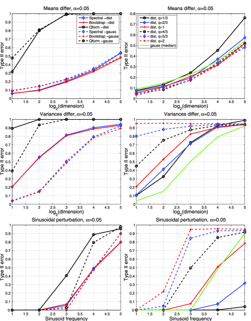
Figure 3: (Left) MMD using Gaussian and distance kernels for various tests; (right) Spectral MMD using distance kernels with various exponents.

=200pt mean var sine Spec 4.66 4.72 5.10 Boot 5.02 5.16 5.20 Qform 0.02 0.05 0.98

Table 1: Type I error (in %) for two-sample tests with distance-induced kernels

We also compare the performance to that of the Gaussian kernel, commonly used in machine learning, with the bandwidth set to the median distance between points in the aggregation of samples. We see that when the means differ, both tests perform similarly. When the variances differ, it is clear that the Gaussian kernel has a major advantage over the distance-induced kernel, although this advantage decreases with increasing dimension (where both perform poorly). In the case of a sinusoidal perturbation, the performance is again very similar.

In addition, following Example 15, we investigate performance of kernels obtained using the semimetric $\rho(z,z^{\prime})=\|z-z^{\prime}\|^{q}$ for $0<q\leq 2$. Results are presented in the right-hand plots of Figure 3. In the case of sinusoidal perturbation, we observe a dramatic improvement compared with the $q=1$ case and the Gaussian kernel: values $q=1/3$ (and smaller) offer virtually error-free performance even at high frequencies [note that $q=1$ yields the energy distance described in Székely and Rizzo (2004, 2005)]. Small improvements over a wider $q$ range are also observed in the cases of differing mean and variance.

We observe from the simulation results that distance-induced kernels with higher exponents are advantageous in cases where distributions differ in mean value along a single dimension (with noise in the remainder), whereas distance kernels with smaller exponents are more sensitive to differences in distributions at finer lengthscales (i.e., where the characteristic functions of the distributions differ at higher frequencies).

8.2 Independence experiments

To assess independence tests, we used an artificial benchmark proposed by Gretton et al. (2008): we generated univariate random variables from the Independent Component Analysis (ICA) benchmark densities of Bach and Jordan (2002); rotated them in the product space by an angle between $0$ and $\pi/4$ to introduce dependence; filled additional dimensions with independent Gaussian noise; and, finally, passed the resulting multivariate data through random and independent orthogonal transformations. The resulting random variables $X$ and $Y$ were dependent but uncorrelated. The case $m=128$ (sample size) and $d=2$ (dimension) is plotted in Figure 4 (left). As observed by Gretton, Fukumizu and Sriperumbudur (2009), the Gaussian kernel using the median inter-point distance as bandwidth does better than the distance-induced kernel with $q=1$. By varying $q$, however, we are able to obtain a wide performance range: in particular, the values $q=1/3$ (and smaller) have an advantage over the Gaussian kernel on this dataset. As for the two-sample case, bootstrap and spectral tests have indistinguishable performance, and are significantly more sensitive than the quadratic form-based test, which failed to detect any dependence on this dataset.

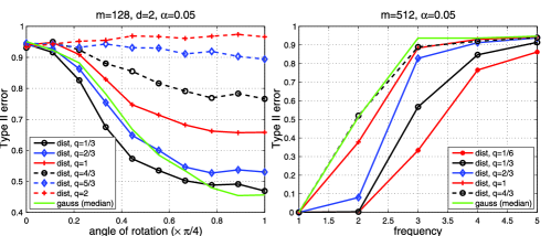
Figure 4: HSIC using distance kernels with various exponents and a Gaussian kernel as a function of (left) the angle of rotation for the dependence induced by rotation; (right) frequency $\ell$ in the sinusoidal dependence example.

In addition, we assess the performance on sinusoidally dependent data. The sample of the random variable pair $X,Y$ was drawn from $P_{XY}\propto 1+\sin(\ell x)\times\sin(\ell y)$ for integer $\ell$, on the support $\mathcal{X}\times\mathcal{Y}$, where $\mathcal{X}:=[-\pi,\pi]$ and $\mathcal{Y}:=[-\pi,\pi]$. In this way, increasing $\ell$ causes the departure from a uniform (independent) distribution to occur at increasing frequencies, making this departure harder to detect given a small sample size. Results are in Figure 4 (right). The distance covariance outperforms the Gaussian kernel (median bandwidth) on this example, and smaller exponents result in better performance (lower Type II error when the departure from independence occurs at higher frequencies). Finally, we note that the setting $q=1$, as described by Székely, Rizzo and Bakirov (2007), Székely and Rizzo (2009), is a reasonable heuristic in practice, but does not yield the most powerful tests on either dataset. Informally, the exponent in the distance-induced kernel plays a similar role as the bandwidth of the Gaussian kernel, and smaller exponents are able to detect dependencies at smaller lengthscales. Poor performance of the Gaussian kernel with median bandwidth in this example is a consequence of the mismatch between the overall lengthscale of the marginal distributions (captured by the median inter-point distances) and the lengthscales at which dependencies are present.

9 Conclusion

We have established an equivalence between the generalized notions of energy distance and distance covariance, computed with respect to semimetrics of negative type, and distances between embeddings of probability measures into certain reproducing kernel Hilbert spaces. As a consequence, we can view energy distance and distance covariance as members of a much larger class of discrepancy/dependence measures, and we can choose among this larger class to design more powerful tests. For instance, Gretton et al. (2012b) recently proposed a strategy of selecting from a candidate kernels so as to asymptotically optimize the relative efficiency of a two-sample test. Moreover, kernel-based tests can be performed on the data that do not lie in a Euclidean space. This opens the door to new and powerful tools for exploratory data analysis whenever an appropriate domain-specific notion of distance (negative type semimetric) or similarity (kernel) can be defined. Finally, the family of kernels that arises from the energy distance/distance covariance can be employed in many additional kernel-based applications in statistics and machine learning, such as conditional dependence testing and estimating the chi-squared distance [Fukumizu et al. (2008)], Bayesian inference [Fukumizu, Song and Gretton (2011)] and mixture density estimation [Sriperumbudur (2011)].

Appendix A Distance correlation

As described by Székely, Rizzo and Bakirov (2007), the notion of distance covariance extends naturally to that of distance variance $\mathcal{V}^{2}(X)=\mathcal{V}^{2}(X,X)$ and of distance correlation (by analogy with the Pearson product-moment correlation coefficient),

$$\mathcal{R}^{2}(X,Y)=\cases{\displaystyle\frac{\mathcal{V}^{2}(X,Y)}{\mathcal{V}(X)\mathcal{V}(Y)},&\quad$\mathcal{V}(X)\mathcal{V}(Y)>0,$\vspace*{2pt}\cr 0,&\quad$\mathcal{V}(X)\mathcal{V}(Y)=0.$}$$

Distance correlation also has a straightforward interpretation in terms of kernels,

$$\mathcal{R}^{2}(X,Y) = \frac{\mathcal{V}^{2}(X,Y)}{\mathcal{V}(X)\mathcal{V}(Y)}$$

$$= \frac{\gamma_{k}^{2}(P_{XY},P_{X}P_{Y})}{\gamma_{k}(P_{XX},P_{X}P_{X})\gamma_{k}(P_{YY},P_{Y}P_{Y})}$$

$$= \frac{\|\Sigma_{XY}\|_{\mathrm{HS}}^{2}}{\|\Sigma_{XX}\|_{\mathrm{HS}}\|\Sigma_{YY}\|_{\mathrm{HS}}},$$

where covariance operator $\Sigma_{XY}\dvtx\mathcal{H}_{k_{\mathcal{X}}}\to\mathcal{H}_{k_{\mathcal{Y}}}$ is a linear operator for which $\langle\Sigma_{XY}f,g\rangle_{\mathcal{H}_{k_{\mathcal{Y}}}}=\mathbb{E}_{XY}[f(X)g(Y)]-\mathbb{E}_{X}f(X)\mathbb{E}_{Y}g(Y)$ for all $f\in\mathcal{H}_{k_{\mathcal{X}}}$ and $g\in\mathcal{H}_{k_{\mathcal{Y}}}$, and $\|\cdot\|_{\mathrm{HS}}$ denotes the Hilbert–Schmidt norm [Gretton et al. (2005)]. It is clear that $\mathcal{R}$ is invariant to scaling $(X,Y)\mapsto(\varepsilon X,\varepsilon Y)$, $\varepsilon>0$, whenever the corresponding semimetrics are homogeneous, that is, whenever $\rho_{\mathcal{X}}(\varepsilon x,\varepsilon x^{\prime})=\varepsilon\rho_{\mathcal{X}}(x,x^{\prime})$, and similarly for $\rho_{\mathcal{Y}}$. Moreover, $\mathcal{R}$ is invariant to translations, $(X,Y)\mapsto(X+x^{\prime},Y+y^{\prime})$, $x^{\prime}\in\mathcal{X}$, $y^{\prime}\in\mathcal{Y}$, whenever $\rho_{\mathcal{X}}$ and $\rho_{\mathcal{Y}}$ are translation invariant. Therefore, by varying the choice of kernels $k_{\mathcal{X}}$ and $k_{\mathcal{Y}}$, we obtain in (A) a very broad class of dependence measures that generalize the distance correlation of Székely, Rizzo and Bakirov (2007) and can be used in exploratory data analysis as a measure of dependence between pairs of random variables that take values in multivariate or structured/non-Euclidean domains.

Appendix B Link with universal kernels

We briefly remark on how our results on equivalent kernels relate to the notion of universal kernels on compact metric spaces in the sense of Steinwart and Christmann (2008), Definition 4.52:

Definition 34.

A continuous kernel $k$ on a compact metric space $\mathcal{Z}$ is said to be universal if its RKHS $\mathcal{H}_{k}$ is dense in the space $C(\mathcal{Z})$ of continuous functions on $\mathcal{Z}$, endowed with the uniform norm.

The family of universal kernels includes the most popular choices in machine learning literature, including the Gaussian and the Laplacian kernel. The following characterization of universal kernels is due to Sriperumbudur, Fukumizu and Lanckriet (2011):

Proposition 35.

Let $k$ be a continuous kernel on a compact metric space $\mathcal{Z}$. Then, $k$ is universal if and only if $\mu_{k}\dvtx\mathcal{M}(\mathcal{Z})\to\mathcal{H}_{k}$ is a vector space monomorphism, that is,

$$\bigl{\|}\mu_{k}(\nu)\bigr{\|}_{\mathcal{H}_{k}}^{2}=\int\int k\bigl{(}z,z^{\prime}\bigr{)}\,d\nu(z)\,d\nu\bigl{(}z^{\prime}\bigr{)}>0\qquad\forall\nu\in\mathcal{M}(\mathcal{Z})\setminus\{0\}.$$

As a direct consequence, every universal kernel $k$ is also characteristic, as $\mu_{k}$ is, in particular, injective on the space of probability measures. Now, consider a kernel $\tilde{k}_{f}$ centered at $f=\mu_{k}(\nu)$ for some $\nu\in\mathcal{M}(\mathcal{Z})$, such that $\nu(\mathcal{Z})=1$. Then $\tilde{k}_{f}$ is no longer universal, since

$$\bigl{\|}\mu_{\tilde{k}_{f}}(\nu)\bigr{\|}_{\mathcal{H}_{\tilde{k}_{f}}}^{2}$$

$$\qquad=\int\tilde{k}_{f}\bigl{(}z,z^{\prime}\bigr{)}\,d\nu(z)\,d\nu\bigl{(}z^{\prime}\bigr{)}$$

$$\qquad=\int\int\biggl{[}k\bigl{(}z,z^{\prime}\bigr{)}-\int k(w,z)\,d\nu(w)-\int k\bigl{(}w,z^{\prime}\bigr{)}\,d\nu(w)$$

$$\qquad\hskip 108.0pt{}+\int\int k\bigl{(}w,w^{\prime}\bigr{)}\,d\nu(w)\,d\nu\bigl{(}w^{\prime}\bigr{)}\biggr{]}\,d\nu(z)\,d\nu\bigl{(}z^{\prime}\bigr{)}$$

$$\qquad=\bigl{(}1-\nu(\mathcal{Z})\bigr{)}^{2}\bigl{\|}\mu_{k}(\nu)\bigr{\|}_{\mathcal{H}_{k}}^{2}$$

$$\qquad=0.$$

However, $\tilde{k}_{f}$ is still characteristic, as it is equivalent to $k$. This means that all kernels of the form (19), including the distance kernels, are examples of nonuniversal characteristic kernels, provided that they generate a semimetric $\rho$ of strong negative type. In particular, the kernel in (17) on a compact $\mathcal{Z}\subset\mathbb{R}^{d}$ is a characteristic nonuniversal kernel for $q<2$. This result is of some interest to the machine learning community, as such kernels have typically been difficult to construct. For example, the two notions are known to be equivalent on the family of translation invariant kernels on $\mathbb{R}^{d}$ [Sriperumbudur, Fukumizu and Lanckriet (2011)].

References

- Alba Fernández, Jiménez Gamero and Muñoz García (2008) {barticle}[mr] \bauthor\bsnmAlba Fernández, \bfnmV.\binitsV., \bauthor\bsnmJiménez Gamero, \bfnmM. D.\binitsM. D. and \bauthor\bsnmMuñoz García, \bfnmJ.\binitsJ. (\byear2008). \btitleA test for the two-sample problem based on empirical characteristic functions. \bjournalComput. Statist. Data Anal. \bvolume52 \bpages3730–3748. \biddoi=10.1016/j.csda.2007.12.013, issn=0167-9473, mr=2427377 \bptokimsref \endbibitem
- Anderson, Hall and Titterington (1994) {barticle}[mr] \bauthor\bsnmAnderson, \bfnmNiall H.\binitsN. H., \bauthor\bsnmHall, \bfnmPeter\binitsP. and \bauthor\bsnmTitterington, \bfnmD. M.\binitsD. M. (\byear1994). \btitleTwo-sample test statistics for measuring discrepancies between two multivariate probability density functions using kernel-based density estimates. \bjournalJ. Multivariate Anal. \bvolume50 \bpages41–54. \biddoi=10.1006/jmva.1994.1033, issn=0047-259X, mr=1292607 \bptokimsref \endbibitem
- Arcones and Giné (1992) {barticle}[mr] \bauthor\bsnmArcones, \bfnmMiguel A.\binitsM. A. and \bauthor\bsnmGiné, \bfnmEvarist\binitsE. (\byear1992). \btitleOn the bootstrap of and statistics. \bjournalAnn. Statist. \bvolume20 \bpages655–674. \biddoi=10.1214/aos/1176348650, issn=0090-5364, mr=1165586 \bptokimsref \endbibitem
- Bach and Jordan (2002) {barticle}[mr] \bauthor\bsnmBach, \bfnmFrancis R.\binitsF. R. and \bauthor\bsnmJordan, \bfnmMichael I.\binitsM. I. (\byear2002). \btitleKernel independent component analysis. \bjournalJ. Mach. Learn. Res. \bvolume3 \bpages1–48. \biddoi=10.1162/153244303768966085, issn=1532-4435, mr=1966051 \bptnotecheck year\bptokimsref \endbibitem
- Baringhaus and Franz (2004) {barticle}[mr] \bauthor\bsnmBaringhaus, \bfnmL.\binitsL. and \bauthor\bsnmFranz, \bfnmC.\binitsC. (\byear2004). \btitleOn a new multivariate two-sample test. \bjournalJ. Multivariate Anal. \bvolume88 \bpages190–206. \biddoi=10.1016/S0047-259X(03)00079-4, issn=0047-259X, mr=2021870 \bptokimsref \endbibitem
- Berg, Christensen and Ressel (1984) {bbook}[mr] \bauthor\bsnmBerg, \bfnmChristian\binitsC., \bauthor\bsnmChristensen, \bfnmJens Peter Reus\binitsJ. P. R. and \bauthor\bsnmRessel, \bfnmPaul\binitsP. (\byear1984). \btitleHarmonic Analysis on Semigroups: Theory of Positive Definite and Related Functions. \bseriesGraduate Texts in Mathematics \bvolume100. \bpublisherSpringer, \blocationNew York. \biddoi=10.1007/978-1-4612-1128-0, mr=0747302 \bptokimsref \endbibitem
- Berlinet and Thomas-Agnan (2004) {bbook}[author] \bauthor\bsnmBerlinet, \bfnmA.\binitsA. and \bauthor\bsnmThomas-Agnan, \bfnmC.\binitsC. (\byear2004). \btitleReproducing Kernel Hilbert Spaces in Probability and Statistics. \bpublisherKluwer, \blocationLondon. \bptokimsref \endbibitem
- Fukumizu, Song and Gretton (2011) {bincollection}[author] \bauthor\bsnmFukumizu, \bfnmKenji\binitsK., \bauthor\bsnmSong, \bfnmLe\binitsL. and \bauthor\bsnmGretton, \bfnmArthur\binitsA. (\byear2011). \btitleKernel Bayes’ rule. In \bbooktitleAdvances in Neural Information Processing Systems (\beditor\bfnmJ.\binitsJ. \bsnmShawe-Taylor, \beditor\bfnmR. S.\binitsR. S. \bsnmZemel, \beditor\bfnmP.\binitsP. \bsnmBartlett, \beditor\bfnmF. C. N.\binitsF. C. N. \bsnmPereira and \beditor\bfnmK. Q.\binitsK. Q. \bsnmWeinberger, eds.) \bvolume24 \bpages1737–1745. \bpublisherCurran Associates, \blocationRed Hook, NY. \bptokimsref \endbibitem
- Fukumizu et al. (2008) {binproceedings}[author] \bauthor\bsnmFukumizu, \bfnmK.\binitsK., \bauthor\bsnmGretton, \bfnmA.\binitsA., \bauthor\bsnmSun, \bfnmX.\binitsX. and \bauthor\bsnmSchölkopf, \bfnmB.\binitsB. (\byear2008). \btitleKernel measures of conditional dependence. In \bbooktitleAdvances in Neural Information Processing Systems \bvolume20 \bpages489–496. \bpublisherMIT Press, \blocationCambridge, MA. \bptokimsref \endbibitem
- Fukumizu et al. (2009) {binproceedings}[author] \bauthor\bsnmFukumizu, \bfnmK.\binitsK., \bauthor\bsnmSriperumbudur, \bfnmB.\binitsB., \bauthor\bsnmGretton, \bfnmA.\binitsA. and \bauthor\bsnmSchoelkopf, \bfnmB.\binitsB. (\byear2009). \btitleCharacteristic kernels on groups and semigroups. In \bbooktitleAdvances in Neural Information Processing Systems \bvolume21 \bpages473–480. \bpublisherCurran Associates, \blocationRed Hook, NY. \bptokimsref \endbibitem
- Gretton, Fukumizu and Sriperumbudur (2009) {barticle}[mr] \bauthor\bsnmGretton, \bfnmArthur\binitsA., \bauthor\bsnmFukumizu, \bfnmKenji\binitsK. and \bauthor\bsnmSriperumbudur, \bfnmBharath K.\binitsB. K. (\byear2009). \btitleDiscussion of: Brownian distance covariance. \bjournalAnn. Appl. Stat. \bvolume3 \bpages1285–1294. \biddoi=10.1214/09-AOAS312E, issn=1932-6157, mr=2752132 \bptokimsref \endbibitem
- Gretton and Györfi (2010) {barticle}[mr] \bauthor\bsnmGretton, \bfnmArthur\binitsA. and \bauthor\bsnmGyörfi, \bfnmLászló\binitsL. (\byear2010). \btitleConsistent nonparametric tests of independence. \bjournalJ. Mach. Learn. Res. \bvolume11 \bpages1391–1423. \bidissn=1532-4435, mr=2645456 \bptokimsref \endbibitem
- Gretton et al. (2005) {bincollection}[mr] \bauthor\bsnmGretton, \bfnmArthur\binitsA., \bauthor\bsnmBousquet, \bfnmOlivier\binitsO., \bauthor\bsnmSmola, \bfnmAlex\binitsA. and \bauthor\bsnmSchölkopf, \bfnmBernhard\binitsB. (\byear2005). \btitleMeasuring statistical dependence with Hilbert–Schmidt norms. In \bbooktitleAlgorithmic Learning Theory (\beditor\bfnmS.\binitsS. \bsnmJain, \beditor\bfnmH. U.\binitsH. U. \bsnmSimon and \beditor\bfnmE.\binitsE. \bsnmTomita, eds.). \bseriesLecture Notes in Computer Science \bvolume3734 \bpages63–77. \bpublisherSpringer, \blocationBerlin. \biddoi=10.1007/11564089_7, mr=2255909 \bptokimsref \endbibitem
- Gretton et al. (2007) {binproceedings}[author] \bauthor\bsnmGretton, \bfnmA.\binitsA., \bauthor\bsnmBorgwardt, \bfnmK.\binitsK., \bauthor\bsnmRasch, \bfnmM.\binitsM., \bauthor\bsnmSchölkopf, \bfnmB.\binitsB. and \bauthor\bsnmSmola, \bfnmA.\binitsA. (\byear2007). \btitleA kernel method for the two-sample problem. In \bbooktitleNIPS \bpages513–520. \bpublisherMIT Press, \blocationCambridge, MA. \bptokimsref \endbibitem
- Gretton et al. (2008) {binproceedings}[author] \bauthor\bsnmGretton, \bfnmA.\binitsA., \bauthor\bsnmFukumizu, \bfnmK.\binitsK., \bauthor\bsnmTeo, \bfnmC. H.\binitsC. H., \bauthor\bsnmSong, \bfnmL.\binitsL., \bauthor\bsnmSchölkopf, \bfnmB.\binitsB. and \bauthor\bsnmSmola, \bfnmA.\binitsA. (\byear2008). \btitleA kernel statistical test of independence. In \bbooktitleAdvances in Neural Information Processing Systems \bvolume20 \bpages585–592. \bpublisherMIT Press, \blocationCambridge, MA. \bptokimsref \endbibitem
- Gretton et al. (2009) {binproceedings}[author] \bauthor\bsnmGretton, \bfnmA.\binitsA., \bauthor\bsnmFukumizu, \bfnmK.\binitsK., \bauthor\bsnmHarchaoui, \bfnmZ.\binitsZ. and \bauthor\bsnmSriperumbudur, \bfnmB.\binitsB. (\byear2009). \btitleA fast, consistent kernel two-sample test. In \bbooktitleAdvances in Neural Information Processing Systems 22. \bpublisherCurran Associates, \blocationRed Hook, NY. \bptokimsref \endbibitem
- Gretton et al. (2012a) {barticle}[mr] \bauthor\bsnmGretton, \bfnmArthur\binitsA., \bauthor\bsnmBorgwardt, \bfnmKarsten M.\binitsK. M., \bauthor\bsnmRasch, \bfnmMalte J.\binitsM. J., \bauthor\bsnmSchölkopf, \bfnmBernhard\binitsB. and \bauthor\bsnmSmola, \bfnmAlexander\binitsA. (\byear2012a). \btitleA kernel two-sample test. \bjournalJ. Mach. Learn. Res. \bvolume13 \bpages723–773. \bidissn=1532-4435, mr=2913716 \bptokimsref \endbibitem
- Gretton et al. (2012b) {binproceedings}[author] \bauthor\bsnmGretton, \bfnmA.\binitsA., \bauthor\bsnmSriperumbudur, \bfnmB.\binitsB., \bauthor\bsnmSejdinovic, \bfnmD.\binitsD., \bauthor\bsnmStrathmann, \bfnmH.\binitsH., \bauthor\bsnmBalakrishnan, \bfnmS.\binitsS., \bauthor\bsnmPontil, \bfnmM.\binitsM. and \bauthor\bsnmFukumizu, \bfnmK.\binitsK. (\byear2012b). \btitleOptimal kernel choice for large-scale two-sample tests. In \bbooktitleAdvances in Neural Information Processing Systems 25 \bpages1214–1222. \bpublisherCurran Associates, \blocationRed Hook, NY. \bptokimsref \endbibitem
- Lyons (2013) {barticle}[author] \bauthor\bsnmLyons, \bfnmR.\binitsR. (\byear2013). \btitleDistance covariance in metric spaces. \bjournalAnn. Probab. \bvolume41 \bpages3284–3305. \bptokimsref \endbibitem
- Müller (1997) {barticle}[mr] \bauthor\bsnmMüller, \bfnmAlfred\binitsA. (\byear1997). \btitleIntegral probability metrics and their generating classes of functions. \bjournalAdv. in Appl. Probab. \bvolume29 \bpages429–443. \biddoi=10.2307/1428011, issn=0001-8678, mr=1450938 \bptokimsref \endbibitem
- Reed and Simon (1980) {bbook}[mr] \bauthor\bsnmReed, \bfnmMichael\binitsM. and \bauthor\bsnmSimon, \bfnmBarry\binitsB. (\byear1980). \btitleMethods of Modern Mathematical Physics. I: Functional Analysis, \bedition2nd ed. \bpublisherAcademic Press, \blocationSan Diego. \bidmr=0751959 \bptokimsref \endbibitem
- Schölkopf, Smola and Müller (1997) {binproceedings}[author] \bauthor\bsnmSchölkopf, \bfnmB.\binitsB., \bauthor\bsnmSmola, \bfnmA. J.\binitsA. J. and \bauthor\bsnmMüller, \bfnmK. R.\binitsK. R. (\byear1997). \btitleKernel principal component analysis. In \bbooktitleICANN (\beditor\bfnmW.\binitsW. \bsnmGerstner, \beditor\bfnmA.\binitsA. \bsnmGermond, \beditor\bfnmM.\binitsM. \bsnmHasler and \beditor\bfnmJ. D.\binitsJ. D. \bsnmNicoud, eds.). \bseriesLecture Notes in Computer Science \bvolume1327 \bpages583–588. \bpublisherSpringer, \blocationBerlin. \bptokimsref \endbibitem
- Sejdinovic et al. (2012) {binproceedings}[author] \bauthor\bsnmSejdinovic, \bfnmD.\binitsD., \bauthor\bsnmGretton, \bfnmA.\binitsA., \bauthor\bsnmSriperumbudur, \bfnmB.\binitsB. and \bauthor\bsnmFukumizu, \bfnmK.\binitsK. (\byear2012). \btitleHypothesis testing using pairwise distances and associated kernels. In \bbooktitleProceedings of the International Conference on Machine Learning (ICML) \bpages1111–1118. \bpublisherOmnipress, \blocationNew York. \bptokimsref \endbibitem
- Smola et al. (2007) {binproceedings}[author] \bauthor\bsnmSmola, \bfnmA. J.\binitsA. J., \bauthor\bsnmGretton, \bfnmA.\binitsA., \bauthor\bsnmSong, \bfnmL.\binitsL. and \bauthor\bsnmSchölkopf, \bfnmB.\binitsB. (\byear2007). \btitleA Hilbert space embedding for distributions. In \bbooktitleProceedings of the Conference on Algorithmic Learning Theory (ALT) \bvolume4754 \bpages13–31. \bpublisherSpringer, \blocationBerlin. \bptokimsref \endbibitem
- Sriperumbudur (2011) {binproceedings}[author] \bauthor\bsnmSriperumbudur, \bfnmB.\binitsB. (\byear2011). \btitleMixture density estimation via Hilbert space embedding of measures. In \bbooktitleProceedings of the International Symposium on Information Theory \bpages1027–1030. \bpublisherIEEE, \blocationPiscataway, NJ. \bptokimsref \endbibitem
- Sriperumbudur, Fukumizu and Lanckriet (2011) {barticle}[mr] \bauthor\bsnmSriperumbudur, \bfnmBharath K.\binitsB. K., \bauthor\bsnmFukumizu, \bfnmKenji\binitsK. and \bauthor\bsnmLanckriet, \bfnmGert R. G.\binitsG. R. G. (\byear2011). \btitleUniversality, characteristic kernels and RKHS embedding of measures. \bjournalJ. Mach. Learn. Res. \bvolume12 \bpages2389–2410. \bidissn=1532-4435, mr=2825431 \bptokimsref \endbibitem
- Sriperumbudur et al. (2008) {binproceedings}[author] \bauthor\bsnmSriperumbudur, \bfnmB.\binitsB., \bauthor\bsnmGretton, \bfnmA.\binitsA., \bauthor\bsnmFukumizu, \bfnmK.\binitsK., \bauthor\bsnmLanckriet, \bfnmG.\binitsG. and \bauthor\bsnmSchölkopf, \bfnmB.\binitsB. (\byear2008). \btitleInjective Hilbert space embeddings of probability measures. In \bbooktitleProceedings of the Conference on Learning Theory (COLT) \bpages111–122. \bpublisherOmnipress, \blocationNew York. \bptokimsref \endbibitem
- Sriperumbudur et al. (2009) {binproceedings}[author] \bauthor\bsnmSriperumbudur, \bfnmB.\binitsB., \bauthor\bsnmFukumizu, \bfnmK.\binitsK., \bauthor\bsnmGretton, \bfnmA.\binitsA., \bauthor\bsnmLanckriet, \bfnmG.\binitsG. and \bauthor\bsnmSchoelkopf, \bfnmB.\binitsB. (\byear2009). \btitleKernel choice and classifiability for RKHS embeddings of probability distributions. In \bbooktitleAdvances in Neural Information Processing Systems 22. \bpublisherCurran Associates, \blocationRed Hook, NY. \bptokimsref \endbibitem
- Sriperumbudur et al. (2010) {barticle}[mr] \bauthor\bsnmSriperumbudur, \bfnmBharath K.\binitsB. K., \bauthor\bsnmGretton, \bfnmArthur\binitsA., \bauthor\bsnmFukumizu, \bfnmKenji\binitsK., \bauthor\bsnmSchölkopf, \bfnmBernhard\binitsB. and \bauthor\bsnmLanckriet, \bfnmGert R. G.\binitsG. R. G. (\byear2010). \btitleHilbert space embeddings and metrics on probability measures. \bjournalJ. Mach. Learn. Res. \bvolume11 \bpages1517–1561. \bidissn=1532-4435, mr=2645460 \bptokimsref \endbibitem
- Sriperumbudur et al. (2012) {barticle}[mr] \bauthor\bsnmSriperumbudur, \bfnmBharath K.\binitsB. K., \bauthor\bsnmFukumizu, \bfnmKenji\binitsK., \bauthor\bsnmGretton, \bfnmArthur\binitsA., \bauthor\bsnmSchölkopf, \bfnmBernhard\binitsB. and \bauthor\bsnmLanckriet, \bfnmGert R. G.\binitsG. R. G. (\byear2012). \btitleOn the empirical estimation of integral probability metrics. \bjournalElectron. J. Stat. \bvolume6 \bpages1550–1599. \biddoi=10.1214/12-EJS722, issn=1935-7524, mr=2988458 \bptokimsref \endbibitem
- Steinwart and Christmann (2008) {bbook}[mr] \bauthor\bsnmSteinwart, \bfnmIngo\binitsI. and \bauthor\bsnmChristmann, \bfnmAndreas\binitsA. (\byear2008). \btitleSupport Vector Machines. \bpublisherSpringer, \blocationNew York. \bidmr=2450103 \bptokimsref \endbibitem
- Székely and Rizzo (2004) {barticle}[author] \bauthor\bsnmSzékely, \bfnmG.\binitsG. and \bauthor\bsnmRizzo, \bfnmM.\binitsM. (\byear2004). \btitleTesting for equal distributions in high dimension. \bjournalInterStat \bvolume5. \bptokimsref \endbibitem
- Székely and Rizzo (2005) {barticle}[mr] \bauthor\bsnmSzékely, \bfnmGábor J.\binitsG. J. and \bauthor\bsnmRizzo, \bfnmMaria L.\binitsM. L. (\byear2005). \btitleA new test for multivariate normality. \bjournalJ. Multivariate Anal. \bvolume93 \bpages58–80. \biddoi=10.1016/j.jmva.2003.12.002, issn=0047-259X, mr=2119764 \bptokimsref \endbibitem
- Székely, Rizzo and Bakirov (2007) {barticle}[mr] \bauthor\bsnmSzékely, \bfnmGábor J.\binitsG. J., \bauthor\bsnmRizzo, \bfnmMaria L.\binitsM. L. and \bauthor\bsnmBakirov, \bfnmNail K.\binitsN. K. (\byear2007). \btitleMeasuring and testing dependence by correlation of distances. \bjournalAnn. Statist. \bvolume35 \bpages2769–2794. \biddoi=10.1214/009053607000000505, issn=0090-5364, mr=2382665 \bptokimsref \endbibitem
- Székely and Rizzo (2009) {barticle}[mr] \bauthor\bsnmSzékely, \bfnmGábor J.\binitsG. J. and \bauthor\bsnmRizzo, \bfnmMaria L.\binitsM. L. (\byear2009). \btitleBrownian distance covariance. \bjournalAnn. Appl. Stat. \bvolume3 \bpages1236–1265. \biddoi=10.1214/09-AOAS312, issn=1932-6157, mr=2752127 \bptokimsref \endbibitem
- Zhang et al. (2011) {binproceedings}[author] \bauthor\bsnmZhang, \bfnmK.\binitsK., \bauthor\bsnmPeters, \bfnmJ.\binitsJ., \bauthor\bsnmJanzing, \bfnmD.\binitsD. and \bauthor\bsnmSchoelkopf, \bfnmB.\binitsB. (\byear2011). \btitleKernel-based conditional independence test and application in causal discovery. In \bbooktitleProceedings of the Conference on Uncertainty in Artificial Intelligence (UAI) \bpages804–813. \bpublisherAUAI Press, \blocationCorvallis, Oregon. \bptokimsref \endbibitem