Stochastic mechano-chemical kinetics of molecular motors:
a multidisciplinary enterprise from a physicist’s perspective
Abstract
A molecular motor is made of either a single macromolecule or a
macromolecular complex. Just like their macroscopic counterparts,
molecular motors “transduce” input energy into mechanical work.
All the nano-motors considered here operate under isothermal
conditions far from equilibrium. Moreover, one of the possible
mechanisms of energy transduction, called Brownian ratchet, does
not even have any macroscopic counterpart. But, molecular motor
is not synonymous with Brownian ratchet; a large number of molecular
motors execute a noisy power stroke, rather than operating as
Brownian ratchet.
We review not only the structural design and stochastic kinetics
of individual single motors, but also their coordination, cooperation
and competition as well as the assembly of multi-module motors in
various intracellular kinetic processes. Although all the motors
considered here execute mechanical movements, efficiency and power
output are not necessarily good measures of performance of some
motors. Among the intracellular nano-motors, we consider the porters,
sliders and rowers, pistons and hooks, exporters, importers, packers
and movers as well as those that also synthesize, manipulate and
degrade “macromolecules of life”. We review mostly the quantitative
models for the kinetics of these motors. We also describe several of
those motor-driven intracellular stochastic processes for which quantitative
models are yet to be developed. In part I, we discuss mainly the methodology
and the generic models of various important classes of molecular motors.
In part II, we review many specific examples emphasizing the
unity of the basic mechanisms as well as diversity of operations
arising from the differences in their detailed structure and kinetics.
Multi-disciplinary research is presented here from the perspective of
physicists.
Keywords:
Motor protein, enzyme, ATP, ion-motive force, myosin, kinesin, dynein,
microtubule, F-actin, helicase, translocase, polymerase, ribosome,
ATP synthase, bacterial flagellar motor.
This is an author-created, un-copyedited final version of the article
published in Physics Reports (©Elsevier).
Submitted to arXiv with the permission of the publisher (Elsevier).
Elsevier is not responsible for any errors or omissions in this version of the manuscript or any version derived from it.
1. Introduction
2. Why should physicists study molecular motors?
Part I: General concepts, essential techniques, generic models and results
3. Motoring on a "landscape": conformation and structure
4. Molecular motors and fuels: classification, catalogue and
some basic concepts
4.1. Classification of molecular machines
4.1.1. Cytoskeletal motors and filaments
4.1.2. Machines for synthesis, manipulation and degradation of
macromolecules of life
4.1.3. Rotary motors
4.2. Fuels for molecular motors
4.2.1. Chemical fuel generates generalized chemical force
4.2.2. Electro-chemical gradient of ions generates ion-motive force
4.2.3. Some uncommon energy sources for powering mechanical work
4.2.4. Manufacturing energy currency from external energy supply
4.3. Some basic concepts
4.3.1. Directionality, processivity and duty ratio
4.3.2. Forcevelocity relation and stall force
4.3.3. Mechano-chemical coupling: slippage and futile cycles
5.Experimental methods for molecular motors:
ensemble-averaged and single-molecule techniques
6. Chemical physics of enzymatic activities of molecular motors:
concepts and techniques
6.1. Enzymatic reaction in a cell:
special features and levels of theoretical description
6.2. Enzyme as a chemo-chemical cyclic machine:
free energy transduction
6.3. Enzymatic activities of molecular motors
6.3.1. Average rate of enzymatic reaction: MichaelisMenten equation
6.3.2. Specificity amplification by energy dissipation:
kinetic proofreading
6.3.3. Effect of external force on enzymatic reactions
catalyzed by motors
6.3.4. Effects of multiple ligand-binding sites:
spatial cooperativity and allosterism in molecular motors
6.3.5. ATPase rate and velocity of motors: evidence for tight coupling?
6.4. Sources of fluctuations in enzymatic reactions and their effects
6.4.1. Fluctuations caused by low-concentration of reactants
6.4.2. Fluctuations caused by conformational kinetics of the enzyme:
dynamicdisorder
6.5. Substrate specificity and specificity amplification
6.5.1. Role of conformational kinetics in selecting specific substrate
6.5.2. Temporal cooperativity in enzymes: hysteretic, mnemonic enzymes
and energy relay
7. Thermodynamics of energy transduction: equilibrium and beyond
7.1. Phenomenological linear response theory for molecular motors:
modes of operation
8. Modeling stochastic chemo-mechanical kinetics:
continuous landscapes vs. discrete networks
8.1. Fully atomistic model, limitations of MD and normal mode analysis
8.2. Coarse-grained model, elastic networks and normal mode analysis
8.3. Stochastic mechano-chemical model: wandering on landscapes
8.3.1. Motor kinetics as wandering in a time-independent
mechano-chemical free-energy landscape
8.3.2. Motor kinetics as wandering in the time-dependent mechanical
(real-space)free-energy landscape
8.4. Markov model: motor kinetics as a jump process in a network of
fully discrete mechano-chemical states
9. Solving the forward problem by stochastic process modeling:
from model to data
9.1. Average speed and loadvelocity relation
9.2. Beyond average: dwell time distribution (DTD)
9.2.1. A matrix-based formalism for the DTD
9.2.2. Extracting kinetic information from DTD
10. Solving the inverse problem by probabilistic reverse engineering:
from data to model
10.1. Frequentist versus Bayesian approach
10.1.1. Maximum-likelihood estimate
10.1.2. Bayesian estimate
10.2. Hidden Markov models
10.2.1. HMM: formulation for a generic model of molecular motor
11. Motoring along filamentous tracks: generic models of porters
11.1. Phenomenological linear response theory and modes of operation
11.2. A generic model of a motor: kinetics on a discrete
mechano-chemical network
11.3. 2-headed motor: generic models of hand-over-hand and inchworm
stepping patterns
12. Sliders and rowers: generic models of filament alignment, bundling
and contractility
13. Nano-pistons, nano-hooks and nano-springs: generic models
13.1. Push of polymerization: generic model of a nano-piston
13.1.1. Phenomenological linear response theory for chemo-mechanical
nano-piston: modes of operation
13.1.2. Stochastic kinetics of chemo-mechanical nano-piston
13.2. Pull of de-polymerization: generic model of a nano-hook
14. Exporters and importers of macromolecules: generic models
15. Motoring along templates: generic models of template-directed
polymerization
15.1. Common features of template-directed polymerization
15.2. A generic minimal model of the kinetics of elongation by
a single machine
15.3. A generic minimal model of simultaneous polymerization by
many machines
16. Rotary motors: generic models
Part II: Kinetic models of specific motors
17. Cargo transport by cytoskeletal motors: specific examples of porters
17.1. Processivei dimeric myosins
17.1.1. Myosin-V: a plus-end directed processive dimeric motor
17.1.2. Myosin-VI: a minus-end directed processive dimeric motor
17.1.3. Myosin-XI: the fastest plus-end directed myosin
17.2. Processive dimeric kinesin
17.2.1. Plus-end directed homo-dimeric porters:
members of kinesin-1 family
17.2.2. Plus-end directed hetero-trimeric porters:
members of kinesin-2 family
17.3. Single-headed myosins and kinesin
17.3.1. Single-headed kinesin-3 family
17.3.2. Single-headed myosin-IX family
17.4. Processive dimeric dynein
17.5. Collective transport by porters
17.5.1. Collective transport of a hard cargo:
load-sharing, tug-of-war and bidirectional movements
17.5.2. Many cargoes on a single track: molecular motor traffic jam
17.5.3. Trip to the tip: intracellular transport in eukaryotic cells
with long tips
17.5.4. Fluid membrane-enclosed soft cargo pulled by many motors:
extraction of nanotubes
17.6. Collective transport of filaments by motors:
non-processivity and bistability
17.7. Section summary
18. Filament depolymerization by cytoskeletal motors:
specific examples of chippers
18.1. Section summary
19. Filament crossbridging by cytoskeletal motors:
specific examples of sliders and rowers
19.1. Acto-myosin crossbridge and muscle contraction
19.2. Sliding of acto-myosin bundle in non-muscle cells: stress fibers
19.3. Sliding MTs by axonemal dynein and beating of flagellai
19.4. Sliding MTs by dynein and platelet production
19.5. Sliding MTs by kinesin-5
19.6. Section summary
20. Push/pull by polymerizing/depolymerizing cytoskeletal filaments:
specific examples of nano-pistons and nano-hooks
20.1.Force generated by polymerizing microtubules in eukaryotes
20.2. Force generated by polymerizing actin: dynamic cell protrusions
and motility
20.2.1. Force generation and cell protrusion by actin polymerization
20.3. Cell polarization: roles of cytoskeletal filaments and motors
20.4. Section summary
21. Mitotic spindle: a self-organized machinery for eukaryotic chromosome
segregation
21.1.Mitotic spindle: inventory of force generators and list of stages
21.1.1. Mitotic spindle: key components and force generators
21.1.2. Mitosis: successive stages of chromosomal ballet
21.2. Spindle morphogenesis
21.2.1. Centrosome-directed astral pathway: search-and-capture
as a first-passage time problem
21.2.2. Chromosome-directed anastral pathways via sliding and sorting
of MTs
21.2.3. Amphitelic attachments: a determinant of fidelity of segregation
21.2.4. Chromosomal congression driven by poleward and anti-poleward
forces
21.2.5. Positioning and orienting spindle: role of MT-cortex coupling
21.3. Pull to the poles
21.3.1. Kinetochore pulling by MT filaments: Brownian ratchet or
power stroke?
21.3.2. Chromosome oscillation
21.3.3. Forceexit time relation: a first passage problem
21.3.4. Chromosome segregation in the anaphase: separated sisters
transported to opposite poles
21.4. Section summary
22. Macromolecule translocation through nano-pore by membrane-associated
motors: specific exporters, importers and packers
22.1. Properties of macromolecule, membrane and medium that affect
translocation
22.2. Export and import of proteins
22.2.1. Bacterial protein secretion machineries
22.2.2. Machines for protein translocation across membranes of
organelles in eukaryotic cells
22.3. Export and import of macromolecules across eukaryotic nuclear envelope
22.4. Export/import of DNA and RNA across membranes
22.4.1. Export/import of DNA across bacterial cell membranes
22.4.2. Machines for injection of viral DNA into host: phage DNA
transduction as example
22.5. Machine-driven packaging of viral genome
22.5.1. Energetics of packaged genome in capsids
22.5.2. Structure and mechanism of viral genome packaging motor
22.6. ATP-binding cassette (ABC) transporters: two-cylinder ATP-driven
engines of cellular cleaning pumps
22.7. ection summary
23. Motoring into nano-cage for degradation: specific examples of nano-scale
mincers of macromolecules
23.1. Exosome: a RNA degrading machine
23.2. Proteasome: a protein degrading machine
23.3. Section summary
24. Polymerases motoring along DNA and RNA templates: template-directed
polymerization of DNA and RNA
24.1. Transcription by RNAP: a DdRP
24.1.1. Effects of RNAPRNAP collision and RNAP traffic congestion
24.1.2. Primae: a unique DdRP
24.2. Replication by DNAP: a DdDP
24.2.1. Coordination of elongation and error correction by a
single DdDP: speed and fidelity
24.2.2. Replisome: coordination of machines within a machine
24.2.3. Coordination of two replisomes at a single fork
24.2.4. Traffic rules for replication forks and TECs: DNAPDNAP and
DNAPRNAP collisions
24.2.5. Initiation and termination of replication: where, which, how
and when?
24.2.6. Genome-wide replication: analogy with nucleation, growth and
coalescence
25. Ribosome motor translating mRNA track: template-directed polymerization
of proteins
25.1. Composition and structure of a single ribosome and accessory devices
25.1.1. Molecular composition and structural design of a ribosome
25.2. Polypeptide elongation by a single ribosome: speed versus fidelity
25.2.1. Selection of amino-acid: two steps and kinetic proofreading
25.2.2. Peptide bond formation: peptidyl transfer
25.2.3. Translocation: two steps of a Brownian ratchet?
25.2.4. Dwell time distribution and average speed of ribosome
25.3. Initiation and termination of translation: ribosome recycling
25.4. Translational error from sources other than wrong selection
25.5. Polysome: traffic-like collective phenomena
25.5.1. Experimental studies: polysome profile and ribosome profile
25.5.2. Modeling polysome: spatio-temporal organization of ribosomes
25.5.3. Effects of sequence inhomogeneity: codon bias
25.6. Summary of sections on machines and mechanisms for template-directed
polymerization
26. Helicase motors: unzipping of DNA and RNA
26.1. Non-hexameric helicases: monomeric and dimeric
26.2. Hexameric helicases
26.3. Section summary
27. Rotary motors I: ATP synthase (F0F1-motor) and similar motors
27.1.Rotary motor F0F1-ATPase
27.1.1. F0 motor: Brownian ratchet mechanism of energy transduction
from PMF during ATP synthesis
27.1.2. F1 motor: power stroke mechanism in reverse mode powered by
ATP hydrolysis
27.1.3. F0 F1 coupling
27.2. Rotary motors similar to F0F1-ATPase
27.2.1. Rotary motor V0 V1 -ATPase: a gear mechanism?
27.2.2. Rotary motor A0A1-ATPase
28.Rotary motors II: flagellar motor of bacteria
28.1. Summary of the sections on rotary motors
29. Some other motors
30. Summary and outlook
Acknowledgments
Appendix A. Eukaryotic and prokaryotic cells: differences in the
internal organization of the micro-factories
A.1. Model eukaryotes and prokaryotes
Appendix B. Molecules of a cell: motor components and raw materials
B.1. Natural DNA, RNA, and proteins
Appendix C. Information transfer in biology: replication, gene expression
and central dogma
Appendix D. Cytoplasmic and internal membranes of a cell
Appendix E. Internal compartments of a cell
Appendix F. Viruses, bacteriophages and plasmids: hijackers or
poor parasites?
F.1. Baltimore classification of viruses according to their genome
Appendix G. Organization of packaged genome: from virus and prokaryotes
to eukaryotes
Appendix H. Experimental methods: introduction to the working principles
H.1. FRET: tool for monitoring conformational kinetics
H.2. Optical microscopy: diffraction-limited and beyond
H.2.1. Diffraction-limited microscopy
H.2.2. Sub-diffraction microscopy (or, super-resolution nanoscopy)
H.3. Single-molecule imaging and single-molecule manipulation
H.4. Determination of structure: X-ray crystallography and
electron microscopy
Appendix I. Modeling of chemical reactions
I.1. Deterministic non-spatial models of chemical reactions:
rate equations for bulk systems
I.1.1. Thermodynamic equilibrium, transient kinetics and
non-equilibrium steady states
I.2. Stochastic non-spatial models of reaction kinetics
I.2.1. Chemical master equation
I.2.2. Chemical Langevin and FokkerPlanck equations
I.3. Enzymatic reactions: regulation by physical and chemical means
Appendix J. Elastic stiffness of polymers
J.1. Freely jointed chain model and entropic elasticity
J.2. Worm-like chain and its relation with freely jointed chain:
persistence length
Appendix K. Cytoskeleton: beams, struts and cables
K.1. Cytoskeleton of eukaryotic cells
Appendix L. Kinetics of nucleation, polymerization and depolymerization
of polar filaments: treadmilling and dynamic instability
References
1 Introduction
All living systems are made of cells. A single cell itself can be an uni-cellular organism whereas multi-cellular organisms consist of different types of cells that communicate and interact with each other, and perform specialized functions. Cells are not only basic structural units but also basic functional units of life [1, 2].
Cell is an “open system”: homeostasis of the “milieux interieur”
The typical size of a cell can very between approximately 1 micron to 10 microns. As the name suggests, a cell is a small compartment that is bounded by a membrane and is filled with an inhomogeneous concentrated aqueous medium containing wide varieties of chemicals. However, a cell is not a bag of “passive” mixture of chemicals. It is an open system that not only exchanges materials with its external environment, but also continues the opposite activities of breaking down and synthesis of its own molecular constituents [3]. In spite of the non-vanishing flux of matter and energy, the internal environment maintains homeostasis (i.e., non-equilibrium stationary state or dynamic equilibrium), a concept which originated in the works of Claude Bernard and William B. Cannon [4, 5].
Molecular motors: “nano-machines” in a “micro-factory”
In this review, we view a cell as a “micro-factory” [7] where operation of the participating nano-machines are well coordinated in space and time. An intracellular nano-machine is either a single macromolecule or a macromolecular complex [7, 8, 9, 10, 11, 12, 13, 14, 15, 16, 17, 18] Just like their macroscopic counterparts, molecular machines have an “engine”, an input and an output.
All the great thinkers from Aristotle to Descartes and Leibnitz compared the whole organism with a machine, the organs being the coordinated parts of that machine. Cell was unknown; even micro-organisms became visible only after the invention of the optical microscope in the seventeenth century. Marcelo Malpighi, father of microscopic anatomy, speculated in the 17th century about the existence molecular machines in living systems. He wrote (as quoted in english by Marco Piccolino [6]) that the organized bodies of animals and plants been constructed with “ very large number of machines”. He went on to characterize these as “extremely minute parts so shaped and situated, such as to form a marvelous organ”. Unfortunately, the molecular machines were invisible not only to the naked eye, but even under the optical microscopes available in his time. In fact, individual molecular machines could be “caught in the act” only in the last quarter of the 20th century. A strong impact across disciplinary boundaries was made by the influential paper of Bruce Alberts [7], then the president of the National Academy of Sciences (USA). He wrote that “the entire cell can be viewed as a factory that contains an elaborate network of interlocking assembly lines, each of which is composed of a set of large protein machines” [7].
If the output of the machine involves mechanical movement, the machine is usually referred to as a motor [19, 20, 21, 22, 23, 24, 25, 26, 27, 28, 29, 30, 31, 32].
However, we’ll use the terms machine and motor interchangeably in this review.
The processes driven by molecular motors include not only intracellular motor transport (as the name might suggest), but also manipulation, polymerization and degradation of the bio-molecules [12, 13, 14]. Molecular motors also drive complex processes like cell motility, mitosis (cell division) and morphogenesis (development of an entire organism). In this review we study the roles of molecular motors in several “vectorial” processes [33] where molecules move, on the average, in a “directed” manner [34, 35, 36, 37].
Beyond inventory; structure, energetics and kinetics
To gain insight into the functions of the molecular motors, it is not enough to prepare just an inventory of their parts or a catalogue of their structural design [38]. In between two successive mechanical steps, a motor transits through a number of chemical states; typical chemical transitions being attachment to and detachment from the track, binding to a fuel molecule, breakdown of the fuel molecule and releasing the resulting product molecules, etc. Besides, a single motor can be capable of performing several different functions. Therefore, to understand the mechanisms of molecular motors one has to study their dynamics during various physico-chemical processes in which they are involved [39]. A comprehensive overview of the operational mechanisms of molecular motors would ultimately emerge from a thorough study of the correlation between their structural design, energetics and stochastic kinetics. However, the major emphasis of this review, which is written from the perspective of statistical physicists, are the energetics and stochastic kinetics of molecular motors. Nevertheless, the prototypical structural designs of motors are sketched at the beginning of our discussion of different types of motors.
Top-down, bottom-up, proximate, ultimate causation: design optimization by tinkering:
To describe the operation of a motor, we may need to use objects at different levels of biological organization, starting from a single molecule to giant supra-molecular aggregates to the entire cell. Therefore, explanation of the operational mechanism of a motor may raise questions of “top-down” and “bottom-up” causation [40]. However, in this review, we’ll not address such philosophical questions.
Explaining the operational mechanism of a motor requires finding the causes of the observed phenomena associated with its operation. Cause and effect can be correlated in biology at different temporal scales [41, 42, 43] Explaining the observed motor-driven “vectorial processes” in terms of the present-day structure and kinetics of the corresponding motor(s) exposes what Ernst Mayr [41] would identify as the “proximate” cause of these phenomena. However, explaining the present-day structure and kinetics of the motors in terms of the evolutionary tinkerings in its design over millions of years reveals what, in Ernst Mayr’s terminology, would qualify as the “ultimate” cause [41]. I believe that the response of a motor to input and its assembly-disassembly can provide us clues as the “proximate” cause of the vectorial processes driven by these motors. In contrast, the evolutionary tinkering of their design thereby, possibly, leading to the adaptive alteration of their function fall in the category of “ultimate” cause of the observed features of vectorial processes that they drive [44, 45].
Unlike man-made macroscopic motors, molecular motors are products of Nature’s evolutionary design over billions of years by tinkering [46]. “Nothing in biology makes sense except in the light of evolution” [47]. In fact, cell has been compared to an “archeological excavation site” [191], the oldest modules of functional devices are the analogs of the most ancient layer of the exposed site of excavation. Does evolution tend to optimize the design of the molecular motors [49]? However, in this review we’ll restrict our discussions mostly to proximate cause at the level of single molecule and supra-molecular assemblies. Occasionally, we’ll mention the names of the evolutionary ancestors of some of the motors.
Wet lab and dry lab: complementary approaches of experiment, theory and computer simulation
Laboratory experiment, theoretical analysis and computer simulations are the three complementary approaches of investigation in physical sciences.
Theory
Laboratory experiment Computer simulations
In biological sciences the divide between the “wet labs” (where experiments are performed) and “dry labs” (where theoretical or computational biologists work) is gradually falling apart and the two communities are meeting at a “moist” zone [50].
Although both theory and experiment are needed to make progress, in this article we critically review mainly the theoretical understanding of the mechanisms of molecular motors. Theory provides understanding and insight. These allow us to formulate hypotheses, systematically organize and interpret the empirical observations, recognize the importance of the various ingredients. Theory also makes it possible to generalize from observations and to create a framework for addressing the next level of question and to make predictions which can be tested by carrying out new experiments. However, as far as possible, we have tried to strike a balance between theory, experiments and computer simulations.
Modeling: deterministic and stochastic, forward and inverse, top-down and bottom-up
Theorization requires a model of the system. A theoretical model is an abstract representation of the real system which helps in understanding the real system [51, 52, 53, 54, 55, 56, 57, 58]. This representation can be pictorial (for example, in terms of cartoons or graphs) or symbolical (e.g., a mathematical model). Qualitative predictions may be adequate for understanding some complex phenomena or for ruling out some plausible scenarios. But, a desirable feature of any theoretical model is that it should make quantitative predictions [56, 59, 54, 55, 60, 61]. Models can be formulated at several levels of biological organization [62, 236, 64, 65], but it should be possible to derive a higher level model by integrating details of a lower level model. Results for a given model can be obtained analytically by mathematical manipulations. But, most often even approximate analytical treatment of realistic models becomes extremely difficult. Results are then obtained by numerical computation [66, 67]. The model can be individual-based or population-based. It can be deterministic or stochastic [68, 69, 70, 71, 72, 73, 74, 75, 76, 77, 78, 79]
The “forward problem” of process modeling [80] starts with a
model that is formulated on the basis of apriori hypotheses which
are, essentially, educated guess as to the mechano-chemical kinetics of
the motor. Standard theoretical treatments of the model yields data on
various aspects on the modeled motor; this approach is expressed below
schematically.
Theoretical model Experimental data
Consistency between theoretical prediction and experimental data validates the model. However, any inconsistency between the two indicates a need to modify the model.
The “inverse problem” of inferring the model from empirical data
has to be based on the theory of probability. Such “statistical
inference” [81] can be drawn by
following methods developed by statisticians over the last one century.
This inverse problem is expressed below schematically.
Theoretical model Experimental data
Inferring the complete network of mechano-chemical states and kinetic scheme of a molecular motor from its observed properties is reminiscent of inferring the operational mechanism of a given functioning macroscopic motor by “reverse engineering” [82, 83]. It would be desirable to follow Platt’s [84] principle of “strong inference” [85] which is an extension of Chamberlin’s [86] “method of multiple working hypothesis” [55]. The relative scores of the competing models (and the corresponding underlying hypotheses) would be a true reflection of their merits. Both the directions of investigations, i.e. the forward problem and the inverse problem are equally important and complementary to each other [87].
Although, because of the usual perspective of statistical physicists, most of the theories reviewed here are based on modeling the kinetic processes, we also explain and review statistical modeling of the experimental data on molecular motors. In the concluding section, we shall summarize our assessment of the achievements and limitations of both these approaches to theoretical studies of molecular motors.
From motor molecules to functional modules: systems biology of molecular motors?
In a living cell, several motors cooperate or coordinate with each other thereby forming “functional modules” [88]. Some functional modules consist of a single assembly whereas the components of other functional modules are dispersed spatially [89]. Thus, each module may be viewed as a “network” of motors and the physiology of an organism may be regarded as a network of networks [90, 91]. Modularity can also increase the robustness of motor [94, 92]. The nature of the forward-inverse problems and the bottom-up, top-down modeling strategies needed for integrating motors at different levels have some similarities, at least in spirit, with those followed in systems biology [94, 95, 96, 97, 98] and in the more ambitious physisome project [99]. However, we’ll consider only a couple of modules, formed by the integration of motors [93], in the part II of this review.
A multidisciplinary enterprise from a physicist’s perspective
(Something there is that doesn’t love a wall, That wants it down. - Robert Frost, in:Mending Wall.)
As a system of scientific investigation, molecular motors are of current interest in several disciplines, e.g., biophysics, biochemistry, molecular cell biology, nanotechnology, etc. Therefore, many papers cited in this review appeared in journals that are not part of the usual list of core journals in physics. Bold and adventurous readers who do not mind browsing journals of other disciplines may find a treasure house of phenomena related to molecular motors that are begging for modeling and explanation.
Organization of this review: parts I and II, appendices
I am fully aware of the challenges of reviewing a multi-disciplinary research topic like molecular motors [100]. As far as possible, I have tried to “provide fresh scientific insight” by carrying out a “novel synthesis” of the results scattered in the primary literature of several different disciplines. However, the presentation has been made from the perspective of a statistical physicist. The review is divided into two parts. In part I we develop the general conceptual foundation and the essential technical framework that are essential for understanding the basic physical principles which govern the operation of molecular motors. In this part the applications of the formalism are restricted to only simple generic models of molecular motors. However, the motivation for these models can be appreciated by browsing the catalogue of the real molecular motors that we present in the beginning of the part I in the form of tables and a brief description.
“The world of life can be studied from two points of view- that of its unity and that of its diversity” [101]. Therefore, in part II we review more detailed models of specific motors and the corresponding kinetic processes. From the catalogues provided in part I, readers may pick and choose motors of their interest and find the corresponding details in the part II. The results summarized in module I emphasize the generic features of molecular motors while the distinct features of different types of motors are presented in module II.
Not all the readers of this review are expected to be familiar with the biological pre-requisites. Therefore, very brief summary of some of the biological facts that are essential for appreciating molecular motors and their functions are presented in the appendices.
2 Why should physicists study molecular motors?
Biomolecular motors operate in a domain where the appropriate units of length, time, force and energy are, nano-meter, milli-second, pico-Newton and , respectively ( being the Boltzmann constant and is the absolute temperature). Aren’t the operational mechanism of molecular motors similar to their macroscopic counterparts except, perhaps, the difference of scale? NO. In spite of the striking similarities, it is the differences between molecular motors and their macroscopic counterparts that makes the studies of these systems so interesting from the perspective of physicists.
Nature of the dominant forces: viscous drag and Brownian force
Force is one of the most fundamental quantities in physics. The forces which dominate the dynamics of molecular motors have negligible effect on macroscopic motors. Consider a solid object of linear size moving through a fluid of density at a speed . The Reynolds number is a dimensionless number that measures the ratio of the inertial and viscous forces acting on the object. On the basis of elementary arguments one can derive [104]
| (1) |
where is the viscosity and is the kinematic viscosity of the fluid. At room temperature, for water . Therefore for a fish [103, 104] of length m moving at a speed of 1 m/s, . In sharp contrast, for a globular protein [19] of radius moving at the same speed of m/s in the same medium, ; it would be even smaller at slower speeds. For a human swimmer, a Reynold’s number of would arise if (s)he tried to swim, for example, in honey! Thus, the dynamics of molecular motors is expected to be dominated by hydrodynamics at low Reynold’s number [105, 106].
The dominant forces acting on a typical Brownian particle are listed
below.
Forces on a Brownian particle
Conservative Dissipative Random
electrostatic force viscous drag thermal force
Already in the first half of the twentieth century D’Arcy Thompson, a pioneer in bio-mechanics, realized the importance of viscous drag and Brownian forces in this domain. He pointed out that in the microscopic world of cells, “gravitation is forgotten” [107] (i.e., inertia is negligible), and “the viscosity of the liquid” and the “molecular shocks of the Brownian movement” as well as the “electric charges of the ionized medium”, have the strongest influence. Thus, the kinetics of molecular motors are dominated by fluctuations and irreversibilities; besides, these exhibit some counter-intuitive phenomena which are characteristics of hydrodynamics at low Reynold’s number.
Energy transduction: isothermal engine far from equilibrium
Molecular motors are made of soft matter whereas macroscopic motors are normally made of hard matter to withstand wear and tear. Nature seems to exploit the high deformability of the “active” soft material [108], of which a molecular motor is made, for its biological function. The special characteristics which make the energy transduction by molecular motors interesting from the perspective of physics are as follows [109]: (i) these motors are isothermal, in contrast to the heat engines of the macroscopic motors [110], (ii) the cycle times of these cyclic motors are finite and the power output is non-zero; the formalisms of neither equilibrium thermodynamics nor endo-reversible thermodynamics [111] are applicable for reasons that we’ll explain later. (iii) Molecular motors operate, in general, under conditions far from thermodynamic equilibrium and, therefore, the formalism of non-equilibrium thermodynamics [112] for coupled mechano-chemical processes is also not applicable. (iv) The energy released by the a single “fuel” molecule is about . Interestingly, the mean thermal energy associated with a molecule at a temperature of the order of , is also . Moreover, equating this thermal energy with the work done by the thermal force in causing a displacement of we get . This is comparable to the elastic force experienced by a typical motor protein when stretched by nm. Thus, a motor protein that gets bombarded from all sides by random thermal forces is similar to a tiny creature getting bombarded randomly from all sides by hailstones! Therefore, the position of its center of mass as well as the positions of its atomic constituents with respect to its center of mass fluctuate. Furthermore, because of the low concentrations of the other molecular species involved in its operation, fluctuations of the cycle time is also another unavoidable intrinsic features of the kinetics of molecular motors. Consequently, in contrast to the deterministic dynamics of the macroscopic motors, the dynamics of molecular motors is stochastic (i.e., probabilistic). Therefore, one has to use the more sophisticated toolbox of stochastic processes and non-equilibrium statistical mechanics for theoretical treatment of molecular motors.
Noise [113] need not be a nuisance for a motor [114]; instead, a motor can move forward by gainfully exploiting this noise. A noise-driven mechanism of molecular motor transport, which does not have any counterpart in the macroscopic world of man-made motors, is closely related to fundamental questions on the foundations of statistical physics.
Spatial symmetry breaking: polar track, directed motility, asymmetric cells
Molecular motors and their respective filamentous tracks not only exhibit intrinsic spatial asymmetries in their key properties, but are also responsible for the spatial organization, including the spatial asymmetries of the emergent patterns, that are observed at the subcellular as well as cellular levels of organization [115].
The cause and effects of broken symmetry of molecular motors can be examined in the broader context of the fundamental principles of symmetry breaking in physics and biology (see the articles in the special “Perspectives on Symmetry Breaking in Biology” [116]). For macroscopic systems in thermodynamic equilibrium, symmetry breaking is explained in terms of the form of the free energy. However, since living cells are far from thermodynamic equilibrium, the theory of symmetry breaking in those systems cannot be based on thermodynamic free energy. As we’ll see repeatedly, kinetics cannot be ignored in the study of symmetry breaking in living systems.
Directed motility of a single motor on a polar track
Energy is a scalar quantity whereas velocity is a vector. How does consumption of energy give rise to a non-zero average velocity of a molecular motor? Moreover, a directed movement that a motor exhibits on the average, requires breaking the forward-backward symmetry on its track. What are the possible cause and effects of this broken symmetry at the molecular level?
As far as the cause of this asymmetry is concerned, the asymmetry of the tracks alone cannot explain the “directed” movement of the motors, because on the same track members of different families of motors can, on the average, move in opposite directions. Obviously, the structural design of the motors and their interactions with the respective tracks also play crucial roles in determining their direction of motion along a track.
Coordination, cooperation and competition of motors: intra-cellular self-organization
Collective dynamics of molecular motors can be viewed at several different levels [117]: (i) coordination of the different subunits of a single motor; (ii) cooperation and competition of a few motors in moving either a single cargo (if they walk on a immobilized filamentous track) or a single filament (if the motors are immobilized and the filament can move); (iii) traffic of a large population of motors on a fibrous network of many filaments; (iv) integration of different types of motors [118] and other energy-transducing force generators within a single modular machinery that performs a specific function.
The size, shape, location and number of intracellular compartments [119, 120, 121, 122, 123] as well as modular intracellular machineries are self-organized [124, 125, 126, 127, 128, 129], rather than self-assembled. Dissipation takes place in “self-organization” and distinguishes it from “self-assembly” [130, 131]; the latter corresponds to the minimum of thermodynamic free energy whereas self-organized system does not attain thermodynamic equilibrium. The coordination, cooperation and/or competition of the “directed” movements of the individual motors on their respective tracks and the push / pull of the other force generators are necessary for the intracellular self-organization process [124, 125].
Cell motility, morphogenesis and development: pattern formation
The broken symmetry at the molecular level, e.g., asymmetric growth kinetics of the polar filaments and the “directed” movement of molecular motors, generate forces required for the motility of a cell as a whole. Moreover, the interplay of the kinetics of motors and the filaments play crucially important roles in cell morphogenesis as well as in the development of an organism, both of which are essentially pattern formation phenomena.
Part I:
General concepts, essential techniques,
generic models and results
“Science is nothing without generalisations. Detached and ill-assorted facts are only raw material, and in the absence of a theoretical solvent, have but little nutritive value. ”- Lord Rayleigh, Presidential address (1884), British Association for the Advancement of Science.
3 Motoring on a “landscape”: conformation and structure
The terms “conformation” and “structure” are used extensively to describe the kinetics of molecular motors. The main aim of this section is to clarify the subtle differences between these two concepts.
The energy landscape of a chemical reaction is a graphical way of showing how the energy of the reacting system depends on the degrees of freedom of the system which include the positions (and orientations) of all the atoms of the reactant and product molecules. For any single event of the occurrence of the reaction, the trajectory in this landscape does not necessarily proceed along the bottom of the valley, but occasionally also makes excursions up the walls of the valley. However, when averaged over large number of such trajectories, the reaction process can be described as an effective route in this landscape that corresponds to the lowest energy from the entrance to the exit over a saddle point. This average route in the multidimensional energy landscape is called the reaction coordinate which we’ll denote by the symbol . Moving along this pathway alters the coordinates of all the atoms involved in the reaction; therefore, this reaction coordinate is actually a composite coordinate. The magnitude of this reaction coordinate expresses how far the reaction has progressed. Often the energy of the system is plotted against the reaction coordinate; the reactants and the products correspond to two local minima separated by a maximum which corresponds to the saddle point on the multi-dimensional energy landscape. The state of maximum energy along the reaction coordinate, is called the transition state. The energy landscape can be surveyed by a detailed quantum chemical calculation [132].
The abundant materials available to nature for designing and manufacturing molecular motors in living cells were proteins and nucleic acids both of which are linear polymers. The individual monomeric residues that form proteins and nucleic acids are amino acids and nucleotides, respectively. Although the monomeric subunits are covalently bonded along the linear chain, the secondary and tertiary structures (and, therefore, the three-dimensional shape) of proteins are determined by much weaker non-covalent bonds (e.g., hydrogen bonds, Van der Waals interactions, etc.) between these chains. Since the strengths of these non-covalent bonds are comparable to the thermal energy , the high-order structures exhibit significant thermal fluctuations even when such “soft” materials are neither subjected to any external force nor participate in any chemical reaction. Thus, proteins are dynamic intrinsically [133].
According to our convention, a conformational state (or, simply, conformation) of a protein is given by the coordinates of all the constituent atoms. In thermodynamic equilibrium, a protein persistently goes through a large number of conformational states which are typically within of the conformation that has the lowest free-energy. If the fluctuations in the positions of the atoms are not too large, we can regard the different conformations as small deviations about a state which is the time-average of these conformations. Such a time-averaged conformational state is called a structural state.
We now explain the relations between conformations and structure more quantitatively [19]. Suppose a protein can exist in any of the different conformational states each with the corresponding potential energy (). Since the conformations are assumed to be canonically distributed in thermodynamic equilibrium, the probability of finding the protein in the -th conformation is
| (2) |
where the partition function is given by
| (3) |
For simplicity, suppose the conformational states segregate into two ensembles where the first is associated with the structural state while the second ensemble is associated with the structural state . For example, and may correspond to the “pre-stroke” and “post-stroke” states of a motor protein. Suppose the first ensemble consists of the conformational states with energies while the remaining conformational states with energies belong the second ensemble. Then, the probability of finding the protein in the structural state is given by
| (4) |
where
| (5) |
is the restricted partition function. Similarly, the probability of finding the protein in the structural state is given by
| (6) |
where
| (7) |
Thus, . But, , where and are the free energies of the structures and , respectively. Hence,
| (8) |
where
| (9) |
Thus, the probability of finding a protein in a conformational state with energy is proportional to whereas that of finding the protein in a structural state with free energy is proportional to . Most of the biological processes, in which molecular motors participate, take place at constant temperature and constant pressure. Therefore, the most appropriate thermodynamic potential (i.e., free energy) is the Gibbs free energy . Therefore, any change of the Gibbs free energy can be expressed as the sum of the contributions from the changes in the enthalpy and entropy : .
For reactions involving two small molecules, for example, the dimension and complexity of the energy landscape are still small enough and the description of the dynamics in this landscape is useful. However, for reactions catalyzed by enzymes (i.e., proteins), manyfold increase in the dimension and complexity of the landscape makes its use cumbersome, if not impractical. However, even for such reactions, a simpler landscape can be constructed by averaging over the fast degrees of freedom which are not important for describing the mechanism of the reaction that takes place on much longer time scales [132, 134, 135]. Such an averaging over a subset of the degrees of freedom yields a “free energy” that still depends on the remaining degrees of freedom; such a “free energy” landscape may be viewed as a projection of the energy landscape onto a much lower-dimensional space. Usually the reaction coordinate is one of the coordinates which span the low-dimensional “free energy landscape”. The cross-section of the free energy landscape along the reaction coordinate is usually plotted as shown in Fig.1 where the deeper of the two local minima corresponds to the products while the other local minimum corresponds to the reactants. The landscape picture and reaction coordinate diagrams are used also to describe the thermodynamics and kinetics of molecular motors [136, 137].

4 Molecular motors and fuels: classification, catalogue and some basic concepts
4.1 Classification of molecular machines
Molecular machines can be classified in many different ways depending on
the characteristic property used for classification.
From the perspective of (mechanical-) engineers, the biomolecular machines
can be classified according to their similarities with their macroscopic
counterparts. Cyclic machines operate in repetitive cycles and are
very similar to the cyclic engines which run our cars. In contrast, some
other molecular machines are one-shot machines that exhaust an
internal source of free energy in a single round.
The most common type of cyclic machines that we’ll consider here
are motors
[19, 22, 23, 24, 25, 26, 27, 28, 29, 32]
and pumps.
In this review we focus exclusively on motors.
So far as the intracellular transport system system is
concerned, its components are as follows:
Intracellular motor transport system = motor + fuel + external regulation & control
motor = engine + transmission system (gear, clutch,etc.)
Therefore, for understanding the intracellular motor transport system, it is not enough to understand the individual motors in isolation. One also needs to pay attention to the regulation of motor transport [138]. However, a detailed discussion of the mechanisms of regulation of molecular motors is beyond the scope of this review.
During its life time, a cell goes through a sequence of different phases before it gets divided into two daughter cells thereby completing one cell cycle. In this review we discuss the energetics and kinetics of molecular motors and motor assemblies which drive key processes during the successive phases of cell cycle.
4.1.1 Cytoskeletal motors and filaments
The cytoskeleton of a cell is the analogue of the human skeleton [19]. However, it not only provides mechanical strength to the cell, but its filamentous proteins also form the networks of “highways” (or, “tracks”) on which cytoskeletal motor proteins [19, 22] can move. Filamentous actin (F-actin) and microtubules (MT) which serve as tracks are “polar” in the sense that the structure and kinetics of the two ends of each filament are dissimilar.
| Motor superfamily | Filamentous track | Minimum step size | Appendix, Section |
|---|---|---|---|
| Myosin | F-actin | 36 nm | K, 17 |
| Kinesin | Microtubule | 8 nm | K,17 |
| Dynein | Microtubule | 8 nm | K,17 |
The superfamilies of cytoskeletal motors and the corresponding filamentous tracks are listed in table 1. These are linear molecular motors because they move along special filamentous linear tracks, performing mechanical work, while consuming some form of (free-) energy input. These are analogs of trains which move on railway tracks. Every superfamily can be further divided into families. Members of every family move always in a particular direction on its track; for example, kinesin-1 and cytoplasmic dynein move towards + and - end of MT, respectively. Similarly, myosin-V and myosin-VI move towards the + and - ends of F-actin, respectively.
For their operation, each motor must have a track-binding site and another site that binds and “burns” a “fuel” molecule (usually hydrolyzes a molecule of Adenosine triphosphate, abbreviated ATP). Both these sites are located, for example, in the head domain of myosins and kinesins. The motor-binding sites on the tracks are equispaced; the actual step size of a motor can be, in principle, an integral multiple of the minimum step size which is the separation between two neighboring motor-binding sites on the corresponding track.
Porters: intracellular cargo transport
Some linear motors are cargo transporters. Such a motor “walks” ‘ for a significant distance on its track carrying the cargo. For obvious reasons, such motors are referred to as porters [139]. The distinct possible stepping patterns of the motor proteins will be discussed in section 11.
Depolymerases: chipping of filamentous tracks
A MT depolymerase is a kinesin motor that chips away its own track from one end [140]. Members of the kinesin-13 family can reach either end of the MT diffusively (without ATP hydrolysis) and, then, start chipping the track from the end where it reaches. In contrast, members of the kinesin-8 family walk towards the plus end of the MT track hydrolyzing ATP and after reaching that end starts chipping it from there. Chipping by both families of depolymerase kinesins are energized by ATP hydrolysis.
Sliders and rowers: motor-filament crossbridge in motility and contractility
| Motor | Sliding filaments | Function (example) | Section |
|---|---|---|---|
| Myosin | “Thin filaments” of muscle fibers | Muscle contraction | 19.1 |
| Myosin | “Stress fibers” of non-muscle cells | Cell contraction | 19.2 |
| Myosin | Cytokinetic “contractile ring” in eukaryotes | Cell division | 29 |
| Kinesin | Interpolar microtubules in mitotic spindle | Mitosis | 21.1 |
| Dynein | Microtubules of axoneme | Beating of eukaryotic flagella | 19.3 |
| Dynein | Microtubules of megakaryocytes | Blood platelet formation | 19.4 |
Some motors are capable of sliding two different filaments with respect to each other by stepping simultaneously on these two filaments [141]. Some sliders work in groups and each detaches from the filament after every single stroke; these are often referred to as rowers because of the analogy with rowing with oars [139, 142]. The oars of rowers come in contact with water for a very brief period, giving a stroke and then comes out of water, completing one cycle. Similarly, “rower” molecular motors also remain attached to their track for a small fraction of their ATPase cycle, i.e., the duty ratio of these nonprocessive motors is usually small. However, the collective stroke of a very large number of such tiny motor molecules can generate forces large enough to slide filaments over a significant distance. Contractility, rather than motility, at the subcellular and cellular level are driven by the sliders and rowers. Some examples of this category are listed in the table 2.
| Polymer | mode of force generation | Function (example) | Section |
|---|---|---|---|
| MT | polymerization | organizing cell interior | 20 |
| F-actin | polymerization | cell motility | 20 |
| FtsZ | polymerization | bacterial cytokinesis | 20 |
| MSP | polymerization | motility of nematode sperm cells | 20 |
| Type-IV pili | polymerization | bacterial motility | 20 |
| MT | de-polymerization | Eukaryotic chromosome segregation | 20 |
| spasmin | spring-like | vorticellid spasmoneme | |
| Coiled actin | spring-like | egg fertilization by sperm cells |
Cytoskeletal polymerizing/depolymerizing filaments: pistons, hooks and springs
Motor proteins are not the only force generators in a cell. In fact, no homolog of motpr proteins have been found so far in prokaryotic cells. Dynamic filamentous proteins also generate forces. Elongation of a filamentous biopolymer that presses against a light object (e.g., a membrane) can result in a “push” [143]. Similarly, a depolymerizing tubular filament can “pull” a light ring-like object by inserting its hook-like outwardly curled depolymerizing tip into the ring [144]. The interplay of the pushing and pulling forces dominate the dynamic organization of the cell interior [145]. A flexible filament, upon compression by input energy, can store energy that can perform mechanical work when the filament springs back to its original relaxed shape [146]. Some typical examples are given in table 3.
The architecture of the diverse MT-based intracellular superstructures are determined by a combined operation of the MT-based motor proteins and other non-motor MT-associated proteins (MAPs) [147, 148, 149, 150, 151, 152, 153, 154]. Similarly, actin-based motor proteins and the non-motor actin-related proteins (ARPs) [155, 156, 157, 158, 159, 160, 161, 162, 163, 164, 165, 166, 167] determine the overall architecture of the actin-based intracellular superstructures. Some of the superstructures self-organized in an in-vitro motor-filament system, in the absence of MAPs and ARPs, will be mentioned in section 21. Microtubule plus-end tracking proteins (+TIPs) [168, 169, 170, 171, 172] are special MAPs that accumulate at the plus end of microtubules; depolymerase motors proteins that target the plus-end of MT filaments are also +TIPs.
4.1.2 Machines for synthesis, manipulation and degradation of macromolecules of life
Membrane-associated motors for translocation of macromolecules across membranes
In many situations, the motor remains immobile and pulls a macromolecule; the latter are often called translocase. Some translocases export (or, import) either a protein [173] or a nucleic acid strand [174, 175] across the plasma membrane of the cell or, in case of eukaryotes, across internal membranes. A list is provided in table 4.
The genome of many viruses are packaged into a pre-fabricated empty container, called viral capsid, by a powerful motor attached to the entrance of the capsid [176].
| Membrane | Polymer | Section |
|---|---|---|
| Nuclear envelope | RNA/Protein | 22 |
| Membrane of endoplasmic reticulum | Protein | 22 |
| Membranes of mitochondria/chloroplasts | Protein | 22 |
| Membrane of peroxisome | Protein | 22 |
Machines for degrading macromolecules of life
Restriction-modification (RM) enzyme defend bacterial hosts against bacteriophage infection by cleaving the phage genome while the DNA of the host bacteria are not cleaved [177]. Exosome and proteasome are nano-cages into which RNA and proteins are translocated and shredded into smaller fragments [178]. Similarly, there are machines for degrading polysachharides, e.g., cellulosome (a cellulose degrading machine) [179], starch degrading enzymes [180], chitinase (chitin degrading enzyme) [181], etc. These machines are listed in table 5.
| Polymer | Examples of Machines | Section/reference |
|---|---|---|
| DNA (polynucleotide) | RM enzyme | [177] |
| RNA (polynucleotide) | Exosome | 23 |
| Protein (polypeptide) | Proteasome | 23 |
| Cellulose (polysachharide) | Cellulosome | [179] |
| Starch (polysachharide) | Starch degrad. enzyme | [180] |
| Chitin (polysachharide) | Chitinase | [181] |
Machines for template-dictated polymerization
Two classes of biopolymers, namely, polynucleotides and polypeptides perform wide range of important functions in a living cell. DNA and RNA are examples of polynucleotides while proteins are polypeptides. Both polynucleotides and polypeptides are made from a limited number of different species of monomeric building blocks, namely, nucleotides and amino acids,respectively. The sequence of the monomeric subunits to be used for synthesis of each of these are dictated by that of the corresponding template. These polymers are elongated, step-by-step, during their birth by successive addition of monomers, one at a time. The template itself also serves as the track for the polymerizer machine that takes chemical energy as input to polymerize the biopolymer as well as for its own forward movement. Therefore, these machines are also referred to as motors.
Depending on the nature of the template and product nucleic acid strands, polymerases can be classified as DNA-dependent DNA polymerase (DdDP), DNA-dependent RNA polymerase (DdRP), etc. as listed in the table 6.
| Machine | Template | Product | Function | Section |
|---|---|---|---|---|
| DdRP | DNA | RNA | Transcription | 24 |
| DdDP | DNA | DNA | DNA replication | 24 |
| RdRP | RNA | RNA | RNA replication | 24 |
| RdDP | RNA | DNA | Reverse transcription | 24 |
| Ribosome | mRNA | Protein | Translation | 25 |
Unwrappers, unzippers and untanglers of DNA: chromatin remodellers, Helicases and topoiomerases
In an eukaryotic cell DNA is packaged in a hierarchical structure called chromatin. In order to use a single strand of the DNA as a template for transcription or replication, it has to be unpackaged either locally or globally. ATP-dependent chromatin remodelers [182] are motors that perform this unpackaging. However, only one of the strands of the unpackaged duplex DNA serves as a template; the duplex DNA is unzipped by a DNA helicase motor [183]. Similarly, a RNA helicase motor unwinds a RNA secondary structure. During DNA replication, a helicase moves ahead of the polymerase, like a mine sweeper, unzipping the duplex DNA and dislodging other DNA-bound proteins. However, the transcriptional and translational machineries do not need assistance of any helicase because these are capable of unzipping DNA and unwinding RNA, respectively, on their own.
In order to control and modulate the DNA topology, a cell uses a class of machines designed specifically for this purpose. These machines, called topoisomerase, can untangle DNA by passing one DNA through a transient cut in another [185].
Quality control: a delicate balance in an unreliable factory
The molecular machines that synthesize the macromolecules in a cell
are far from perfect. Therefore, template-directed polymerization
is an error-prone process. Any defective protein is likely to misfold
and, therefore, would be unsuitable for its biological function.
Misincorporation of a nucleotide during the polymerization of a mRNA
would produce an erroneous template for protein synthesis. Error in
DNA replication would produce defective genome for the daughter cells.
In order to maintain macromolecular integrity, each cell has a
“quality-control system” [184]. In the context of molecular
machines for synthesis and degradation of macromolecular machines, the
following questions are of fundamental interest: (i) does the quality
control system detect the perfect product or the defective product?
(ii) Does this detection take place during the ongoing polymerization
process (e.g, immediately after committing an error) or after the
product molecule is released by the machinery at the end of synthesis
of the complete product?
(iii) Is the detection mechanism based on the principles of equilibrium
thermodynamics or kinetics?
(iv) Once an error is detected, is the error corrected or is the
defective product degraded?
(v) What are the possible short-term and long-term consequences of
an error if the error escapes detection or/and correction/degradation
process of the quality control system?
Although in this review we focus exclusively on the machines and
mechanisms that ensure high quality of the macromolecular products,
the quality-control system of a normal eukaryotic cell acts on
multiple levels- molecular, organellar as well as cellular levels
[184].
4.1.3 Rotary motors
Rotary molecular motors [186] (see table 7) are, at least superficially, very similar to the motor of a hair dryer. Two rotary motors have been studied most extensively. (i) A rotary motor embedded in the membrane of bacteria drive the bacterial flagella which, the bacteria use for their swimming in aqueous media. (ii) A rotary motor, called ATP synthase is embedded on the membrane of mitochondria, the powerhouses of a cell. A synthase drives a chemical reaction, typically the synthesis of some product; the ATP synthase produces ATP, the “energy currency” of the cell, from ADP.
4.2 Fuels for molecular motors
Energy sources available not only explain the differences in the “lifestyles” of prokaryotes and eukaryotes [187] but also provides an alternative perspective on the fundamental question of the origin of life [188]. It is thermodynamics and kinetics which ultimately decided the allowed processes that led to the emergence of life from inanimate matter. Throughout the subsequent evolution of life, energy has fuelled the machineries in living systems [189]. Therefore, this aspect of the investigations on molecular machines is intimately related to the subject of bioenergetics [190, 191, 192].
Several polymerase motors are capable of extracting the required input energy directly from the substrates that they use for polymerizing a macromolecule. On the other hand, some motors that degrade nucleic acids are powered by the free energy released by the degrading nucleic acid strand. However, motors that use filamentous polymers as track use a separate fuel molecule; in most cases the fuel molecule is adenosine tri-phosphate (ATP). Contributions to the input energy for a motor come from (a) the binding of ATP, (b) hydrolysis of the bound ATP molecule, as well as (c) release of the products of hydrolysis.
4.2.1 Chemical fuel generates generalized chemical force
Before considering any specific chemical reaction that provides the input chemical energy for a specific motor, let us keep the discussion as general as possible. We consider the reaction
| (10) |
where higher energy compound gets converted to the lower energy compound spontaneously. The forward and reverse fluxes are given by and , respectively. In thermodynamic equilibrium of this system,
| (11) |
i.e.,
| (12) |
where , and hence . What happens if the concentrations of and deviate slightly from the equilibrium concentrations? The populations of the two molecular species keep changing by conversion from one species to the other till the new concentrations again satisfy the equilibrium condition (11). What drives the system towards equilibrium and which way does this proceed- forward or reverse?
In order to address the question posed at the end of the last paragraph, suppose, there are molecules of (each of free energy ) and molecules of (each of free energy ). The corresponding free energy of the entire system is given by
| (13) |
If one molecule of now gets converted to one molecule of by the reaction (10), the new free energy of the system can be obtained from (13) by replacing and by and , respectively. Let us denote the corresponding change in the free energy of the entire system by . When and are sufficiently large, it is straightforward to show that
| (14) |
Comparing eqn.(14) with eqn.(12), we find that vanishes in equilibrium. Moreover, indicates merely the direction of spontaneous conversion of a molecule with high free energy into a molecule of low free energy. But, when the concentrations of the molecules deviate from equilibrium, it is that drives the chemical system towards equilibrium. Furthermore, change in the free energy caused by the conversion of one molecule is identical to the change in the chemical potential . Therefore, we define as the “generalized chemical force” .
Example 1: ATP hydrolysis vs. ATP synthesis
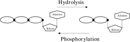
The most common way of supplying energy to a natural nano-motor is to utilize the chemical energy (or, more appropriately, free energy) released by a chemical reaction. Most of the motors use the so-called “high-energy compounds”- particularly, nucleoside triphosphates (NTPs)- as an energy source to generate the mechanical energy required for their directed movement. However, the term “high-energy compound”, although widely used colloquially, is confusing. Here “high-energy” or “energy-rich” merely means that the free energy change associated with the chemical reaction, that the compound undergoes to supply input (free-)energy for the motor, is strongly negative [194]. The most common chemical reaction is the hydrolysis of ATP to ADP (see fig.2). ATP analogoues [195] are very useful substitutes for normal ATP for exploring the role of ATP in the operational mechanism of a molecular motor.
Some other high-energy compounds can also supply input energy; one typical example being the hydrolysis of Guanosine Triphosphate (GTP) to Guanosine Diphosphate (GDP). Inorganic pyrophosphate (PPi), which forms naturally during the hydrolysis of ATP into Adenosine mono-phosphate (AMP) by the reaction ATP AMP + PPi, is also used as fuel in some living systems [196, 197]. Interestingly, PPi is a member of the family of inorganic polyphosphates [198, 199] which are believed to be an ancient energy source in living systems.
A curiosity in the choice of phosphates as the energy currency of the cell: why did Nature choose phosphates? This question can be answered only by examining its relative stability and its enhanced rate of hydrolysis by the enzymes as compared to alternative compounds which might have been available to Nature during the course of evolution. It has been argued [200] that phosphates were the best choice for Nature but, perhaps, not for the present-day organic chemists.
If a cyclic machine runs on a specific chemical fuel then the spent fuel must be removed as waste products and fresh fuel must be supplied to the machine. Fortunately, normal cells have machineries for recycling waste products to manufacture fresh fuel, e.g., synthesizing ATP from ADP. This raises an important question: since ATP is a higher-energy compound than ADP, how are the ATP-synthesizing machines driven to perform this energetically “uphill” task? Fortunately, chemical fuel is not the only means by which input energy can be supplied to intracellular molecular machines; ATP synthesis is driven by ion-motive force (IMF) that we discuss in the next subsubsection.
4.2.2 Electro-chemical gradient of ions generates ion-motive force
During Darwinian evolution, cells seem to have selected only two atomic species of ions for the electro-chemical gradient- hydrogen ion (which is is essentially a single proton) and sodium ion . The evolutionary advantages of these two ionic species over all other possible candidates and the sequence in which these might have been selected in the course of evolution are still debated but will not be discussed here [201, 202, 203, 204, 205, 206, 207].
An electro-chemical gradient of protons across the membrane of a cell or that of an organelles of an eukaryotic cell generates the proton-motive force (PMF). The strength of the PMF is generally expressed in terms of the free energy required to create it. Suppose denotes the electric potential and is the concentration of the protons (hydrogen ions). Traditionally, in the literature on active transport across membranes [192, 193] is expressed as
| (17) |
where the subscripts and refers to inside and outside of the membrane-bound compartment, is the Faraday constant and is the gas constant ( where is the Avogadro number). The first and second terms on the right hand side of (17) correspond to the concentration (chemical) gradient and electrical potential gradient, respectively. Since and since equation (17) can also be recast in terms of the pH values on the two sides of the membrane. A similar expression describes the sodium-motive force (SMF) generated by the electro-chemical gradient of sodium ions [208].
4.2.3 Some uncommon energy sources for powering mechanical work
The spring-like action of spasmoneme is powered neither by any NTP nor by any IMF. Instead, binding of Ca2+ ions causes contraction of the spring thereby storing elastic energy that is later released when the spring rapidly extends to its full length because of the unbinding of the calcium ions [146]. Similarly, the switching of a forisome from a spindle-like elongated shape to a balloon-like swollen plug is energized also by the binding of calcium ions [209, 210, 211, 212]. In living plants movements can be caused by the variation of internal pressure (also called turgor) of cells that arise from uptake or loss of water [213]. However, we’ll not discuss these mechanisms of force generation in this review.
For designing artificial nanomotors, light is often the preferred choice as the input energy. The advantages of using light, instead of chemical reaction, as the input energy for a molecular motor are as follows: (i) light can be switched on and off easily and rapidly, (ii) usually, no waste product, which would require disposal or recycling, is generated.
4.2.4 Manufacturing energy currency from external energy supply
A cell gets its energy from external sources. It has special machines to convert the input energy into some “energy currency”. For example, chemical energy supplied by the food we consume is converted into an electro-chemical potential that not only can be used to synthesize ATP, but can also directly run some other machines. In plants similar proton-motive forces are generated by machines which are driven by the input sunlight.
Thus, study of molecular machines deals with two complementary aspects of bioenergetics: (a) conversion of energy input from the external sources into the energy currency of the cell, and (b) utilization of the energy currency to drive various other active processes [194].
ATP was discovered by Lohmann and, independently, by Fiske and Subbarow [214, 215, 216]. As we will discuss in section 27, synthesis of ATP from ADP is driven by a PMF (or, SMF). But, the mechanism of generating the PMF (and, SMF) from metabolic energy was discovered by Peter Mitchell [217, 218, 219, 220, 221, 222]. For the history of the discoveries of the reaction chains that convert other forms of input energy into the standard energy currencies of the cell, see ref.[223, 224]).
4.3 Some basic concepts
4.3.1 Directionality, processivity and duty ratio
All the members of a distinct family of motor protein moves in a specific direction on its track which is a polar filament, i.e, whose two ends are not equivalent. One of the key features of the kinetics of molecular motors is their ability to attach to and detach from the corresponding track. A motor is said to be attached to a track if at least one of its domains remains bound to the corresponding track.
One can define processivity in three different ways:
(i) Average number of chemical cycles in between attachment and
the next detachment from the filament;
(ii) attachment lifetime, i.e., the average time in between an
attachment and the next detachment of the motor from the filament;
(iii) mean distance spanned by the motor on the filament in
a single run.
The first definition is intrinsic to the process arising from the
mechano-chemical coupling. But, it is extremely difficult to
measure experimentally. The other two quantities, on the other
hand, are accessible to experimental measurements.
Leibler and Huse [139] presented a unified scenario for the
function of the cytoskeletal motor proteins and argued that the different
processivities of the motors arise from the different rate limiting
processes in their mechano-chemical cycle. The details of their
arguments will be examined in part II.
To translocate processively, a motor may utilize one of the three
following strategies:
Strategy I: the motor may have more than one track-binding domain
(oligomeric structure can give rise to such a possibility quite
naturally). Most of the cytoskeletal motors, like conventional two-headed
kinesin, use such a strategy. One of the track-binding sites remains
bound to the track while the other searches for its next binding site.
Strategy II: A motor may possess non-motor extra domains or some
accessory protein(s) bound to it which can bind to the track even when
none of the motor domains of the motor is directly attached to the track.
Strategy III: it can use a “clamp-like” device to remain attached
to the track; opening of the clamp will be required before the motor
detaches from the track. Many motors utilize this strategy for moving
along the corresponding nucleic acid tracks.
During one cycle, suppose a motor spends an average time bound (attached) to the filament, and the remaining time unbound (detached) from the filament. Clearly, the period during which it exerts its working stroke is and its recovery stroke takes time . The duty ratio, , is defined as the fraction of the time that each head spends in its attached phase, i.e.,
| (18) |
4.3.2 Force-velocity relation and stall force
An external force that opposes the natural directed movement of a motor is called a load force. As the strength of the load force is increased, the average velocity of the motor decreases. The force-velocity relation is one of the most important characteristics of a molecular motor; its status in the studies of molecular motors is comparable to that of the I-V characteristics of a device in the studies of semiconductors. The minimum load force which just stalls the motor is called the stall force and it is the true measure of the maximum force that a motor can generate.
The force-velocity relation can have the general form [225]
| (19) |
where is the average velocity of the motor in the presence of a load force and is the stall force. Both the unloaded velocity and the stall force are important measurable characteristics of a motor. The magnitude of determines the curvature of the plot. For example, corresponds to a linear force-velocity relation. In contrast, sub-linear and super-linear force-velocity relations, which arise for and , respectively, appear convex-up and concave-up when plotted graphically.
What happens to the motor if it is subjected to a load force that is
stronger than the stall force? Clearly, there are three possibilities:
(a) the motor may simply detach from the track;
(b) the motor may walk backward (i.e., in a direction that is opposite
to its natural direction of motion in the absence of any load force),
but this motion is driven by the load force alone because the motor
no longer hydrolyzes any “fuel” molecule;
(c) the motor walks backward, but is hydrolyzes “fuel” molecules
exactly the same way as it does while moving forward for load forces
. Can a motor synthesize, instead of hydrolyzing, ATP
while walking under the action of load force opposite to
its natural direction of motion? We shall see in part II that, different
families of motors exercise different options among (a), (b) and (c) above.
The load force need not be directed exactly parallel to the filament.
Consequences of vectorial loading of molecular motors have also been
investigated [226, 639]
4.3.3 Mechano-chemical Coupling: slippage and futile cycles
A molecular motor has to coordinate its three cycles: (a) enzymatic cycle in which it hydrolyzes one molecule of the “fuel” (ATP or GTP); (ii) cycle of attachment to- and detachment from the track; and (iii) stepping cycle in which it moves forward or backward on the track by one mechanical step.
In this context, some of the fundamental questions on the nature and
strength of the mechano-chemical coupling are as follows:
(i) how many cycles of hydrolysis of ATP (or GTP) occurs during a
single cycle of mechanical stepping of the motor?
(ii) Is “slippage” between the chemical cycle of ATP (or GTP)
hydrolysis and the mechanical cycle of stepping possible? In other
words, is it possible that hydrolysis of fuel turns out to be “futile”
in the sense that it does not lead to any stepping of the motor?
For such motors, the output is loosely coupled to the input; the output
work extracted from the same amount of input energy (e.g., hydrolysis
of a single ATP molecule) fluctuates from one cycle to another
[228].
This is in sharp contrast the output of macroscopic motors are usually tightly coupled to the corresponding input; the chemical energy is converted into mechanical work via a strictly scheduled sequence of stages where in each stage there is one-to-one correspondence between the movements of the parts of the motor and the work done. We define the strength of the coupling by
| (20) |
where is the step size. Note that is the probability that the motor takes a mechanical step in space per chemical reaction. Tight coupling corresponds to whereas all if the coupling is loose. Moreover, if the motor can take more than one mechanical step per cycle of chemical reaction.
5 Experimental methods for molecular motors: ensemble-averaged and single-molecule techniques
Most of the traditional experimental techniques of biophysics and biochemistry relied on collection of data for a large collection of molecules and thereby getting their ensemble-averaged properties. The amplification of the signals caused by the presence of large number of such molecules makes it easier to detect and collect the data. However, there are practical limitations of the bulk measurements in the specific context of understanding the operational mechanisms of cyclic molecular machines because it is practically impossible to synchronize their cycles. That’s why single-molecule techniques are required. The single molecule of interest also acts like a reporter of the local “nano-environment” because its own properties are influenced by those of the molecules in its immediate surroundings [229].
Thus, experimental techniques for probing the operational mechanisms of molecular motors can be divided broadly into two groups [230]:
Experimental techniques
Ensemble-averaged Single-molecule
The advantages of single-molecule techniques are as follows: (a) Single molecule imaging exposes the inhomogeneity and disorder in a sample even when the dynamic inhomogeneities average out over longer period of time, (b) enable the observer to monitor a molecule as it moves in a complex fluid medium, (c) probe the kinetics of the molecule and reveal even the rare pathways which would not be detected in the ensemble-averaged measurements over bulk systems, while the single-molecule techniques of manipulation, in addition, yield (d) quantitative measures of forces, distances and velocities. The basic principles of some of the most useful techniques are summarized in appendix H.
6 Chemical physics of enzymatic activities of molecular motors: concepts and techniques
The input (free-) energy of chemo-mechanical molecular motors is derived from chemical reactions. Therefore, in order to understand the mechanisms of bio-molecular motors, it is necessary to understand not only how these move in response to the mechanical forces but also how these are affected by generalized “chemical forces”. Enzymes and ribozymes constitute two classes of biological catalysts; enzymes are proteins whereas ribozymes are RNA molecules. As we’ll illustrate in parts II, most of the molecular motors considered here are either enzymes or consist of ribozymes. Therefore, it is desirable to have some background knowledge in the theory of enzymatic reactions before embarking on a study of bio-molecular motors.
For any motor that doesn’t step backwards, the position of its center of mass advances in the forward direction by one step at a time. Similarly, if a single enzyme molecule catalyzes a chemical reaction that is practically irreversible, the population of the product molecules increases by one in each enzymatic cycle. In recent years this formal analogy between mechanical stepping and enzymatic reaction has enriched the fields of biophysics and chemical biology by exchange of novel ideas. Molecular motors have the unique distinction of involving both these phenomena in its core mechanism of operation. The main aim of this section is to provide a brief summary of the essential concepts and techniques for studying enzymatic reactions, particularly in the context of molecular motors.

Two classes of enzymes that are most relevant in the context of molecular motors are the (i) ATPases (which hydrolyze ATP), and (ii) GTPases (which hydrolyze GTP) [231]. For obvious reasons, proposals have been made to include these NTPases in one single class and to name the class an “energases” [232] although this proposal has been criticised [232].
Even for a given single motor domain, a large number of chemical states are involved in each enzymatic cycle. In principle, there are, many pathways for the hydrolysis of ATP, i.e., there are several different sequences of states that defines a complete hydrolysis cycle. Although, all these pathways are allowed, some paths are more likely than others. The most likely path is identified as the hydrolysis cycle. Let us consider an ATPase, an enzyme that hydrolyzes ATP (see Fig.3). Under normal conditions, the spontaneous rate of hydrolysis of ATP extremely low. However, ATPases are enzymes which specifically speed up this reaction.
6.1 Enzymatic reaction in a cell: special features and levels of theoretical description
All chemical reactions are intrinsically reversible and have the general form Reactants Products. However, if the rate of the reverse reaction is very small compared to that of the forward reaction, or if the products are continuously removed from the reaction chamber as soon as thes are formed, the reaction becomes, effectively, irreversible and takes the form Reactants Products. Chemical kinetics is a framework for studying how fast the amounts of reactants and products change with time.
Special features of enzymatic reactions in-vivo
How do chemical reactions within cells differ from those occuring in-vitro? (i) First, because of the dense crowd of molecules in a solution, the reactions take place in the presence of a “background” that occupies a large fraction of the cell itself. Consequently, even if this background does not participate actively in the reaction, it can (a) shift the equilibrium concentrations of the reactants and the products, and (b) change the reaction rates [233, 234, 235]. For example, the reactant and/or product molecules may be adsorbed reversibly and non-specifically on a nearby fiber or membrane that is a constituent of this “background”; such adsorption can influence the course of the reaction. A concrete example is that of a molecular motor that hydrolyzes ATP; the rate of ATP hydrolysis depends on whether or not the motor is interacting with a filamentous track. (ii) Second, interior of a cell is so inhomogeneous that the rate of the same biochemical reaction may vary significantly depending on the location of the reaction. (iii) Third, for many reactions inside a cell, the population of the reactants can be so low that rate of the reaction may fluctuate strongly from one instant to another, even at the same spatial location. For example, the duration of the ATPase cycle of a molecular motor is a fluctuating quantity.
Levels of description in theories of chemical reactions
Rate equations: deterministic ODEs; no spatial fluctuation- well-stirred approximation
Reaction-diffusion equations: deterministic PDEs; spatial variations captured
Chemical master- or chemical Fokker-Planck/Langevin equations: stochastic description
Quantum-mechanical theories (quantum chemistry)
Modelling the electronic processes through which chemical bonds are made and broken would require a quantum mechanical formalism. However, our interest in this article is restricted to phenomena which occur on length scales longer than the spatial extent of the molecules and on time scales longer than those of electron dynamics. The effects of the electronic degrees of freedom get averaged out on the length and time scales of our interest. Therefore, we do not present here the quantum mechanical formalisms of chemical reaction kinetics.
Theory of chemical reactions can be developed at several different levels depending on the purpose of the investigation [236, 75, 237]. Moreover, at a given level, the equations can be formulated at least in two different ways: (i) equations which govern the time evolution of the populations of the molecular species involved in the reaction, (ii) equations which describe the motion of individual molecules [238]. Furthermore, equations for chemical kinetics are often developed ignoring the possibility of spatial variations. However, spatial variations in the populations of the reactants and products can be taken into account, for example, by replacing the ordinary differential equations by partial differential equations. Finally, depending on the physical situation and the level of description, the equations of chemical kinetics can be either deterministic or stochastic. (A brief technical summary of these alternative formulations of chemical reaction kinetics is presented in appendix I).
6.2 Enzyme as a chemo-chemical cyclic machine: free energy transduction
A general cyclic reaction can be written as
| (21) |
In this section we show how cyclic chemical reaction can be exploited to design a chemo-chemical machine for which both input and output are chemical energies [239, 240]. Such machines are chemical analogues of simple mechano-mechanical machines like a simple lever.
In order to motivate the design of a chemo-chemical machine, consider a reaction
| (22) |
which is strongly favored as the corresponding change of free energy . On the other hand, the reaction
| (23) |
is weakly unfavored as the corresponding . So, given an opportunity, molecules will spontaneously transform to whereas molecules will spontaneously transform into . Is it possible to utilize the large change of free energy of the first reaction (22) to drive the second reaction (23)? If this is possible, this would be an example of “free energy transduction” and system would operate as a chemo-chemical machine. Some of the free energy released in the reaction (22) is, then, used to pay the free energy cost required to drive the unfavorable reaction (23).
On many occasions it is hard to see how the two reaction would couple together to transduce the free energy on their own. On the other hand, free energy transduction is quite common in living cells; in these processes, usually, a large protein molecule or a macromolecular complex plays the role of a “broker” or a “middleman”. In fact, most of the molecular motors we consider here fall in this category of “brokers”.
Example of a chemo-chemical machine

To illustrate the mechanism let us consider a hypothetical (but, in principle, possible) model shown in fig.4 where is the enzyme. Note that exists in this model in two different conformational states, denoted by and , which are interconvertible. There is one binding site for and another for on the same conformation of the enzyme. On the other hand, in the conformational state of the enzyme, these binding sites are accessible only to the molecules and . Therefore, once and bind to their respective binding sites on , the enzyme makes a transition to the state forcing and to make the corresponding transitions to and , respectively.

Thus, in this model, the enzyme exists in six states numbered by the sequence of integers shown in fig.4. If one enzyme completes one cycle in the clockwise (CW) diretion, the net effect is to convert one molecule and one molecule into one molecule and one molecule; the enzyme itself is not altered by the complete cycle.
With the use of only one cycle, as shown in fig.4, there is tight coupling between the two reactions (22) and (23), i.e., the stoichiometry is exactly one-to-one: each complete cycle coverts exactly one and one into exactly one and one molecule.
Fig.5 is a generalization of the model where possible transitions between and are now also included. This small extension has non-trivial consequences as we shall explain below. Note that now there are three possible cycles as shown in the figure 6. The possible directions are chosen arbitrarily in the CW direction in all three cycles. As explained above, cycle (a) transduces free energy. The cycle (b) runs spontaneously; but, from the point of view of free energy transduction, this cycle does not contribute and it simply dissipates some of the free energy of . The cycle (c), which runs opposite to the direction of spontaneous progress of the reaction, is an wasteful cycle from the perspective of free energetics. Only the cycle (a) transduces free energy. However, if all the cycles (a), (b) and (c) occur, the cycles (b) and (c) spoil the exact stoichiometry thereby reducing the overall efficiency of the free energy transduction. More precisely, if the transitions between and occur, the tight coupling of the model is lost because of the “slippage” caused by the cycles (b) and (c) converting the model into a “weak-coupling” model. Thus, for free energy transduction, the kinetic diagram must have at least one cycle that involves both free energy supply and free-energy demanding transitions.
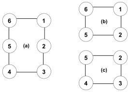
An appropriate measure of the efficiency of the free energy transduction in any chemo-chemical machine is given by
| (24) |
For the abstract chemo-chemical machine designed above,
| (25) |
6.3 Enzymatic activities of molecular motors
Although, for appreciating the mechanisms of molecular motors, one has to be familiar with the enzymatic activities of only the motors, we present the basic principles from a much broader perspective [241, 242, 243]. Implications of the rate of the enzymatic activities of a motor for its mechanical movements will be examined repeatedly in this review for the generic models as well as for the models of specific motors.
6.3.1 Average rate of enzymatic reaction: Michaelis-Menten equation
It has been felt for a long time that the scenario depicted in fig.1 is an oversimplified description of chemical reactions, particularly those which are catalyzed by enzymes. A specific reactant molecule, after diffusing in the medium, comes sufficiently close to the enzyme to bind reversibly forming an enzyme-reactant complex . Then, converts to the enzyme-product complex catalytically and thereafter dissociates whereby the product is released; the free enzyme is available again for the next cycle. This scheme can be represented as follows:
For such a simple scheme, the counterpart of the fig.1 would be as shown in fig.7 which exhibits more maxima and minima than those in Fig.1.
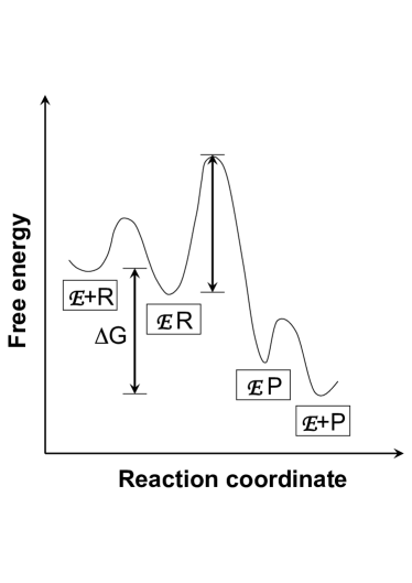
In a more general situation, the conformation of the enzyme immediately after releasing the bound ligands may not be identical to its original relaxed ligand-free conformation . Such situations can be captured by generalizing the scheme (LABEL:eq-MMscheme0) to
| (27) |
If the rate of conversion is sufficiently rapid, can be approximated by and the scheme (27) would reduce to the form (LABEL:eq-MMscheme0). Often a simpler reaction scheme of the type [244]
| (28) |
is adeqate where the symbol represents an intermediate molecular complex and it is assumed to yield and irreversibly. For the sake of simplicity, we have assumed only a single intermediate state , the treatment can be easily extended if more than one intermediate states are involved in the reaction, for example,
| (29) |
A derivation of MM equation under steady-state assumption
For the enzymatic reaction
| (30) |
which does not distinguish between and , the rate equations are
| (31) |
| (32) |
| (33) |
Moreover, as the total amount of enzyme is, by definition, conserved, we must have
| (34) |
We now make two simplifying assumptions.
Assumption 1: , i.e., the second step is
practically irreversible; this condition can be implemented by
removing the products from the reaction chamber as soon as these
are released by the enzyme in each enzymatic cycle.
Then, the equation (33) simplifies to
| (35) |
Eliminating from (32) and (34) we get
| (36) |
Assumption 2: (steady-state approximation) for the intermediate complex , i.e., . This situation arises if, for example, , i.e., the reactants are in large excess, compared to the total initial amount of enzyme. We can now envisage a situation where, during a very brief initial period, the intermediate complex is formed and soon its concentration attains a steady (i.e., time-independent) value. For all successive times, the rate of conversion of into the product and free enzyme can exactly balance the rate of formation of thereby maintaining the steady concentration of
| (37) |
Moreover, assuming to be practically constant (because there is so much excess of R), , indeed, reaches the above mentioned steady state with a relaxation time
| (38) |
starting from .
Under these assumptions, the speed of the reaction is
| (39) |
which is conventionally expressed in the form
| (40) |
where the so-called Michaelis constant
| (41) |
is the ratio of the total rates of reactions out of and that into .
We’ll now explore the physical meaning and significance of the Michaelis constant . Writing , we find that as , where is the maximum possible reaction rate. Therefore, the equation (40) can be recast as
| (42) |
From (42) we see that for , , i.e., is the reactant concentration at which the reaction rate is half of its maximum possible value.
A derivation of MM equation under quasi-equilibrium approximation
In order to get further insight into the MM equation, let us make a “quasi-equilibrium” (i.e., near equilibrium) approximation where the first step
is assumed to attain equilibrium whereas the rate of the second step
is assumed to be very small (infinitesimal). Then, for the first step (note that from the consideration of free energetics, is the reactant and and are the products),
| (43) |
No product formation is possible if this equilibrium is strictly maintained. However, suppose the deviation from equilibrium is extremely small so that the equation (43) still holds approximately. Then the rate of product formation is given by
| (44) |
which, formally, appears similar to (40) except that replaces ; the difference between the two can be made as small as one wishes by reducing accordingly.
Analysis of experimental data and testing validity of MM scheme
Two important parameters which characterize the MM equation are
and . Several different methods of curve plotting
has been followed in the literature to extract these two parameters
from the experimental data.
(i) According to the equation (42), which is also called
Lineweaver-Burk equation, plotting experimentally measured values
of against , one should get a straight line with slope
and intercept from which both and
can be extracted.
(ii) Alternatively, equation (42) can be recast as
| (45) |
Therefore, plotting against , one can get and
using the slope and intercept of the straight line.
(iii) A third alternative is to use the form
| (46) |
of the same equation (42) to extract and from the slope and intercept of the straight line obtained by plotting against . Critical analysis of the available experimental data indicate that the rates of a large class of enzymatic reactions do not follow the MM equation [245]. For a critical evaluation of the assumptions made in deriving the MM equation and the reliability of the methods of estimating and from the experimental data using the above scenario, see ref.[246, 78]. The validity of the steady-state assumption and the possibility of extending the domain of its validity have been examined critically over the last few decades (see, for example, ref.[247, 248, 249, 250, 251, 252, 253]).
6.3.2 Specificity amplification by energy dissipation: kinetic proofreading
Enzymes are specific in the sense that every reaction is catalyzed by a specific enzyme. Machines for template-directed polymerization, that also qualify as molecular motors (reviewed in sections 15, 24, 25), select monomeric subunits of the growing polymer at every step as directed by the corresponding template. The fidelity of the polymerization process depends, at least in part, on the accuracy of this selection of the substrate that is then enzymatically bonded to the growing polymer. In this section we discuss a particular mechanism of specificity amplification, called kinetic proofreading [254, 255], that enhances accuracy beyond what would be normally allowed from purely thermodynamic considerations.
Suppose an enzyme E catalyzes specifically both the reactions and . Now consider a situation where, is the desired product of the reaction catalyzed by E because is needed for some specific biological function. However, both and are present so that the enzyme molecules can catalyze both the reactions thereby producing both the correct product and the wrong product . The lowest free energy of the enzyme-reactant complex along the reaction pathway is expected to be lower than that of the complex by an amount . Therefore, the smallest ratio of the populations of the wrong and correct products is expected to be . If the two reactants are very similar, may not be sufficiently large to keep below a certain pre-determined tolerance level of error.
Kinetic proofreading is a kinetic mechanism designed for specificity amplification, e.g., for decreasing the fraction of population of the erroneous product to (or, in general, to with ). Let us assume that the catalytic reactions with both the correct and incorrect substrates follow the Michaelis-Menten scheme 27. For simplicity, we also assume that all the rate constants, except , are identical for both the substrate species, i.e., the substrate discrimination arises only from the differences between and . For simplicity, we also present the arguments under the quasi-equilibrium approximation although the general conclusions are valid also for the more realistic steady-state approximation. Then, the average rates of the corresponding reactions, in the quasi-equilibrium approximation, are
| (47) |
where and . We define to be the ratio of the rates of formation of the wrong and correct products. For the same initial concentrations of the two substrates, i.e., , we get . So, with pure MM-scheme of the enzymatic reaction the substrate discrimination is limited by the free energy different between the two.
Next, let us consider the kinetic scheme shown below
| (48) |
which is an extension of the MM scheme; in this extended version an extra intermediate state and a branched path from have been added. This scheme is one of the simplest possible implementations of kinetic proofreading [254, 255]. In this assuming that the rate of the transition to be extremely small compared to that for the transition along the branched pathway , one gets where is the ratio of the rates of formation of wrong and correct products according to the scheme (48).
Kinetic proofreading amplifies substrate specificity beyond what
is allowed purely on the basis of equilibrium thermodynamics.
The two features are essential for kinetic proofreading are
as follows [256, 257, 258]:
(i) a strongly forward driven step that results in a high-energy
intermediate complex, and
(ii) one or more branched pathways along which dissociation of
the enzyme-reactant complex, and rejection of the reactant, can
take place before the complex gets an opportunity to make the final
transition to yield the product.
Many other mechanisms of specificity amplification have been proposed. One of these, based on “energy relay” will be discussed later in this section. Another kinetic proofreading scheme [259] is based on “inter-molecular frustration”.
6.3.3 Effect of external force on enzymatic reactions catalyzed by motors
External force affect not only mechanical movements over significant distances, but also alter the rates of chemical reactions in each cycle of a molecular motor. The effects of force on enzymatic reactions catalyzed by motor proteins have been investigated extensively [260, 261], particularly after single-molecule techniques were developed [262, 263, 264, 265].
The free energy landscape is altered by an external force; it affects not only the equilibrium populations of the various structural states, but also the rates of transitions among these states. [260, 261, 262, 264, 265] For the purpose of explaining these phenomena, let us again consider the reaction (287). Suppose an external force is applied on the protein and the force is directed from to . Then
| (49) |
where is the free energy difference between and in the absence of the external force . Obviously, in equilibrium,
| (50) |
i.e., the structural state is more probable than the state .
The equation (50) implies that we can write the individual rate constants for the forward and reverse transitions as [260, 261, 262, 264]
| (51) |
and
| (52) |
where is a fraction of the distance and determines
how the external load is shared by the forward and reverse transitions.
The forms of
-dependence assumed in (51) and (52) is
used routinely for molecular motors while deriving their force-velocity
relations which are among the fundamental characteristics of each
family of motors.
6.3.4 Effects of multiple ligand-binding sites: spatial cooperativity and allosterism in molecular motors
The term “cooperativity” is used to describe wide variety of biochemical phenomena. Cooperative interactions involving proteins can take place at various levels of organization [266]: (a) intra-molecular interaction between different regions of the same protein (e.g., in a monomeric enzyme), (b) inter-molecular interaction between the different protein molecules of an oligomeric single enzyme, (c) inter-enzyme interactions in a multi-enzyme complex, etc.
In the context of enzymes and motors, the term “cooperativity” refers to a process in which one event affects another event of similar type (e.g., binding of a ligand) by means of intra-molecular (in a single protein) or inter-molecular (in a multi-protein macromolecular complex) communication. For example, several types of motors have more than one binding sites for ATP. Almost all motors have multiple binding sites also for other ligands. Linear motors must also have a binding site for attaching to the track. The emergent properties of such motors are results of the “cooperative” effects.
Cooperativity in enzymatic kinetics has been studied extensively over several decades [267, 268, 269, 270, 271, 272, 273]. Quantitative measure of cooperativity can be defined both in terms of thermodynamic equilibrium and kinetics. The increase (or decrease) of binding of one ligand following that of another can be quantified in terms of free energies of binding. If the binding of the first ligand helps (inhibits) the binds of the second, the cooperativity is called positive (negative) If the two ligands are of the same type, the cooperativity is homotropic whereas heterotropic cooperativity involves two different types of ligands. Both homotropic and heterotropic cooperativity can be either positive or negative.
In the context of enzymatic reaction kinetics, usually non-Michaelis-Menten behavior of an enzyme is identified as the signature of cooperativity. However, more objective quantitative measures of the extent of cooperativity have been used in the literature [271]. What is the reason for identifying MM kinetics as a non-cooperative phenomenon? Note that for independent trials of a biased coin, for which head and tail occur with probabilities and , respectively, the expected number of heads is . Comparing this form with the average rate of MM reaction, we conclude that the form (40) is a signature of non-cooperativity.
When plotted graphically, the crucial difference between the MM-type equation and the Hill-type equation is that the curvature of the former is negative for all whereas, for all that of the latter changes sign from positive to negative with gradual increase of . A Hill-type form would be an indicator of cooperativity; and indicate positive and negative cooperativities, respectively (see fig.8).

The interaction between the ligands is not direct. Instead, conformational changes in the enzyme following the binding of one ligand influences the binding of another ligand to the same enzyme. Past history of occupation of a ligand-binding site can propagate temporally, and affect the binding of ligands to the same enzyme in future, if conformation of the enzyme does not relax to the original conformation of free enzyme before the next round of ligand-binding [269, 270, 271]. We’ll consider temporal cooperativity in the context of molecular motors later in this section. Alternatively, information on the occupational status of one binding site can be transmitted spatially to the other binding site(s).
For an enzyme with at least two binding sites the phenomenon of spatial cooperativity leads to the interesting cooperative phenomenon of allosterism [274]. Allostery is a mechanism for regulation of the structure, dynamics and function of an enzyme by the binding of another molecule, called effector, which can be a small molecule (a ligand) or another macromolecule [275, 276, 277, 278, 279, 280, 281, 282]. The three defining characteristics of allostery are [283]: (i) the effector is chemically distinct from the substrate, (ii) the binding site for the effector is spatially well separated from that of the substrate, and (iii) binding of an effector molecule affects at least one of the functional properties of the enzyme; the functional property could be either (a) the binding affinity for its specific substrate or (b) the rate of the reaction it catalyzes.
The models of allosteric control were originally analyzed within the framework of equilibrium thermodynamics [275, 276]. Over the last decade, a more general mathematical formulation of this phenomenon has been reported [284, 285, 286, 287]. Unlike deterministic picture of the thermodynamic formulation, this statistical mechanical theory allows spontaneous fluctuations and introduces the concept of conformational spread (CS). The CS model postulates that each subunit of the enzyme can be in either an active or an inactive conformation and can make rapid transitions between these states. In this model, an individual subunit can also bind a ligand present in the surrounding solution. The probability of a subunit being active or inactive depends on (i) whether or not it is bound to a ligand, and (ii) the conformational state of its neighbors. This model may be regarded as an extension of the Ising model which is one one of the simplest models in equilibrium statistical mechanics [288]. The properties of this CS model have been derived using the formal techniques which are widely used for analyzing the Ising model. The CS model reduces to the two pioneering models [275, 276] of allosteric control in two different special limits.
Allosterism is not restricted only to proteins; allosteric ribozymes are also receiving attention in recent years [289]. A motor protein has separate sites for binding the fuel molecule and the track. Therefore, the mechano-chemical cycle of a motor can be analyzed from the perspective of allosterism [290, 286, 291]. The cycles of molecular motors can be represented as a sequence of allosteric transitions which are caused by the binding or release of fuel molecules (e.g., ATP) and the spent fuel (e.g., ADP and ) as well as attachment and detachment of the filamentous track. Typical generic cycles in the absence and in the presence of the corresponding track are shown in fig.9. Presence of track has very significant effects on the ATP binding and hydrolysis. There are some common features of the enzymatic cycle of cytoskeletal motors, in spite of some crucial differences [292].

6.3.5 ATPase rate and velocity of motors: evidence for tight coupling?
If ATP hydrolysis fuels the mechanical movement of a molecular motor, is there a direct relation between this ATPase rate and the average velocity of the motor on its track? For example, is the ATP-dependence of the average velocity governed by a MM-like equation when the average rate of ATP hydrolysis, by the same motor, follows MM-equation? If so, does this MM-like form survive even when the motor is subjected to a load force ? If it does, then the MM-like form of the force-dependent average velocity of a motor would be [608, 293, 294]
| (53) |
where is the strength of mechano-chemical coupling (defined by eqn.(20)) and is the step size of the motor. The -dependence of both the characteristic parameters and are mentioned explicitly in (53). Since, apriori, the mechano-chemical coupling of molecular motors is expected to be weak, one curiosity is to find out whether any motor displays tight-coupling (i.e., ). All these fundamental questions have been addressed in the last decades by many careful experiments and sophisticated analysis of the data; in part II we’ll find answers to these questions in the context of specific molecular motors.
6.4 Sources of fluctuations in enzymatic reactions and their effects
Apart from drawing input energy from enzymatic reactions, some motors also catalyze other types of chemical reactions. For example, a DdDP, whose main function is template directed polymerization of a DNA molecule, also catalyzes DNA cleavage for error correction. Therefore, understanding the causes and consequences of the fluctuations in enzymatic reactions is required for getting a broader picture of the performance of some motors.
To my knowledge, a stochastic treatment of the MM scheme of enzymatic reactions was published already in 1962 by Bartholamay [2197]. In this pioneering work, he made clear distinction between “two types of irreproducibilities”: those arising from experimental noise and those caused by intrinsic fluctuations. He also emphasized that “even in the total absence of experimental irregularities a concentration time course has an independent existence as a statistical entity” [2197]. With remarkable clarity, Bartholomay [2197] identified the sources of these fluctuations to be the “Brownian-like motions of the reactant molecules”, the “random intermolecular collisions”, and the accompanying intramolecular (i.e., conformational) transitions.
Sources of fluctuations in enzymatic reactions
Let us now summarize the sources of fluctuations in enzymatic reactions.
There are at least three different sources which might contribute
to the fluctuations in the turnover times [295]:
(i) intrinsic stochasticity arising from the reservoir that provides
the thermal energy required for barrier crossing;
(ii) low concentration of the reactants makes the arrival of the
substrate molecules to the enzyme stochastic; and
(iii) Conformational fluctuations of the enzyme can introduce novel
features which are absent when the catalyst is a rigid molecule.
6.4.1 Fluctuations caused by low-concentration of reactants
Micro-macro correspondence: MM equation in thermodynamic limit
Let us consider an enzymatic reaction which is given by the scheme
| (54) |
Suppose there is a single enzyme molecule and substrate molecules in a reaction volume. If can be maintained strictly constant at all times by inserting a substrate molecule whenever one gets converted to product, the MM equation describes the average rate of the reaction. But, if the substrate concentration is allowed to fluctuate around a constant mean, i.e., =constant, deviation of the average rate of the reaction from the corresponding MM equation is found [296]. Not surprisingly, the average rate of the reaction approaches the MM equation in the “thermodynamic limit” (see fig.10).
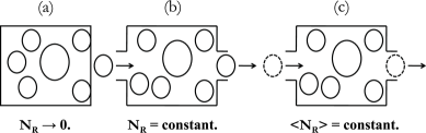
Single-molecule enzymology: turnover time and average rate
Single-molecule enzymology [297] is relevant also for understanding single-motor mechanism. The time needed to complete one catalytic cycle of an enzyme is called its turnover time. The inverse of the mean turnover time gives the average rate of the reaction. Each turnover consists of the following stages:
Substrate selectionproduct formationrelease of product & enzyme relaxation
Therefore, the turnover time should be the sum of the times taken for each of these stages.
Let us compare and contrast various types of assays that can be used for enzymology [298, 299]. Suppose the numbers of enzymes and reactant molecules are denoted by and , respectively. In biochemical experiments on enzymatic reactions using bulk samples, usually, ; for example reactants can be in micro-molar range while the enzyme may be in nano-molar range. This scenario can be described as “multiple enzyme, multiple turnover” because each of the enzyme molecule goes through multiple rounds of enzymatic cycle. In general, the cycles of different enzyme molecules are not synchronized and the population of the product molecules increases smoothly, and linearly, with time.
However, if , and if the reaction is not too fast, each enzyme molecule will catalyze the reaction only once; this scenario may be described as “multiple enzyme, single turnover”. In this case, the population of the product molecules increases smoothly within a period of time and, then, saturates as all the reactants are exhausted and fully converted to the product.
In contrast, if , the enzyme goes through many rounds of enzymatic cycle in this “single enzyme, multiple turnover” scenario. The population of the product molecules increases by unity in each cycle of the enzyme and the turnover time fluctuates randomly.
We now show that, in spite of the fluctuations of the turnover times [300] the average rate may still satisfy MM equation [301, 302, 305, 303, 304, 306]. Consider the MM reaction scheme [301]
| (55) |
where is the reactant and is the product of the reaction catalyzed by while is the same enzyme in an excited state. In the limit the reaction scheme (55) reduces to the original reaction scheme (27) for which we derived the MM equation (42) using reaction rate equation approach.
| (56) |
| (57) |
| (58) |
where
| (59) |
We assume that is independent of time ; this is a good approximation because the reaction is driven by one single enzyme molecule whereas the initial amount of the reactant is sufficiently large. Note that probability that one reaction has been completed in the time interval between and probability that the enzyme molecule was not in the state upto time and is in the state between and probability that at time the enzyme molecule was in state and made a transition to in the next time interval . Thus,
| (60) |
Moreover, as the total amount of enzyme is, by definition, conserved, we must have
| (61) |
We solve the equations (56)-(58), with the constraint (61), using the initial conditions
| (62) |
Hence,
| (63) |
where
| (64) |
| (65) |
Distribution of turnover times: generic features of first and second moments
Substituting (63) into the definition
| (66) |
of the mean turnover time and relating it with the average rate of the reaction by , we recover the MM equation (42) for .
Next, let us begin with the oversimplified linear enzymatic reaction scheme, with distinct kinetic states, where all the transitions (i) are completely irreversible, and (ii) take place with the same rate . For this scheme the distribution of the turnover times is the Gamma-distribution
| (67) |
where is the gamma function. Interestingly, for the Gamma-distribution, the randomness parameter [307] (also called the Fano factor [308])
| (68) |
is exactly given by . Therefore,
| (69) |
provides a strict lower bound on the number of kinetic states [310].
For a very general class of kinetic schemes, which can be interpreted either as that of an enzymatic reaction or as that of a molecular motor, Moffitt et al.[310] derived a very general expression for that has a status similar to the MM-expression for . Their derivation was based on the assumptions that (i) the scheme is a linear chain without branching or parallel pathways, (ii) the last step of the transitions is irreversible, and (iii) obeys the MM equation. Under these assumptions, they derived [310]
| (70) |
which involves, in addition to the Michaelis constant , three dimensionless parameters , and . In spite of the difference in the details of the kinetic schemes, all of which satisfy the assumptions made in the derivation of eqn.(70), the corresponding can be expressed in terms of and exactly as in (70). However, the actual functional dependence of these parameters on the rate constants depends on the details of the kinetic scheme. Note that and . Moreover, occurrence of a maximum or minimum in at some intermediate concentration of the substrate depends on the magnitude of as compared to those of and .
6.4.2 Fluctuations caused by conformational kinetics of the enzyme: “dynamic disorder”
While dealing with fluctuations of enzymatic reactions, so far we have not paid any attention to the conformational kinetics of the enzymes. In general, the conformational dynamics of proteins [133] span a wide range of length and time scales- from a fraction of nanometer to tens of nanometers and from femtoseconds to seconds, or even longer [314]. What makes the study of this dynamics so challenging is the coupling between the motions that occur on a hierarchy of time scales which, in turn, is a consequence of a hierarchy of energy barriers. Conformational fluctuations of a enzyme gives rise to temporal fluctuations in the reaction rates of an enzyme molecule; this randomness is called “dynamic disorder” [315, 316].
Irreversible decay as an example:
In order to get an intuitive analytical understanding of the effects of interconversion of motor (or, enzyme) conformations, one can begin, alternatively, with a discrete formulation of the reaction [317]
where and are two distinct conformations of the same motor (or, enzyme). The reaction considered here could be, for example, the decay of the fluorescent state to a non-fluorescent state. The rate of the decay, however, is assumed to depend on the conformation of the fluorescent state, i.e., in general . Initially, the protein can be either in or in with the probabilities and , respectively. Let and denote the probabilities of finding the protein in the conformations and , respectively, at any arbitrary time .
First consider the special case where no interconversion of the conformations and is allowed on the time scale of the decay. Solving the corresponding master equations
| (72) |
under the initial conditions and , we get and . Hence, the survival probability
| (73) |
Now let us allow reversible interconversion of the conformations and with the same rates for the forward and backward transitions, as shown in eqn(LABEL:eq-xie) [317, 318]. The equations (72) are modified to
| (74) |
In this case is still a sum of two terms each of which decays exponentially with but, in contrast to the decay rates and in (73), the decay rates of the two exponentials are . In the limit and , and .
In this and the next few subsections, we explore the roles of the
conformational kinetics of enzymes [319]
(i) on the turnover times;
(ii) in generating temporal correlations, if any, between
the times taken for its catalytic cycles in a multiple turnover
and enzymatic hysteresis,
(iii) in the selection of specific substrates and specificity
amplification.
Conformational kinetics of enzymes have been studied following two
alternative mathematical approaches. One of these visualizes the
kinetics as wandering in an energy landscape whereas the other
represents kinetics in terms of jumps on a discrete network of states.
This classification of the approaches is summarized below emphasizing
that the two are related to each other.
Mathematical formalisms for conformational kinetics of enzymatic reactions
Wandering in an energy landscape jumping around on a discrete network
Conformational dynamics as wandering in an energy landscape
Let us portray the reaction on a two-dimensional landscape where the two axes quantify the “reaction coordinate” and “conformational coordinate” while the height at each point is a measure of the corresponding free energy [320, 321] (see fig.11) This free energy diagram resembles a model of a mountain range and is obtained by averaging over all the other degrees of freedom which correspond to faster dynamics. Each local minimum in the two-dimensional free energy landscape corresponds to a distinct conformational state. Fluctuations of length scales much shorter than inter-minima separation and on time scales much shorter than the time required for hopping from one local minimum to a neighboring one manifest as vibrations around the corresponding local minimum [322]. Usually, the barriers separating the successive minima along the conformational coordinate are relatively low and, therefore, can be overcome by thermal activation on relatively short time scales. In contrast, the barriers to be crossed along the reaction coordinate are usually much higher and, therefore, the reaction proceeds at a slower rate.
As discussed earlier, in the older picture, a catalytic cycle consists of a sequence of intermediate enzyme-substrate or enzyme-product complexes along the reaction coordinate. In the current scenario, the free enzyme, as well as these intermediate complexes, exist as an ensemble of conformations along the conformational coordinate [319]. Thus, what appears as an effectively unique transition state in fig.1 turns out to be the “transition state ensemble” [323] on this two-dimensional landscape. This ensemble of transition states forms a plane, which resembles a stretch of high “mountain peaks” and runs perpendicular to the reaction coordinate, bisects the diagram. Reactants (and the enzyme-reactant complexes) are on one side of this plane while the products (and enzyme-product complexes) are on the other side [320, 324].
If the conformational dynamics are much faster than the reaction, then for a given value of the reaction coordinate, an ensemble-average over the conformational coordinate yields projection of the free-energy landscape onto the reaction coordinate. However, for many enzymatic reactions, barriers in both the directions are of comparable height. For such reactions, multiple pathways on this two-dimensional landscape are available for the reaction to occur.
Let us first consider two extreme limiting cases. (a) First consider the scenario where the “mountain peak range” running perpendicular to the reaction coordinate are much higher than small “hills” on the two sides of this range. In this limit, because of the fast conformational transitions, the enzyme-reactant complex explores all possible conformations before its conversion to enzyme-product complex. Consequently, the one-dimensional free energy profile obtained by the projection of the two-dimensional free energy landscape onto the reaction coordinate provides an adequate description of the reaction. Classical treatment of enzymatic reactions in terms of the MM scheme (or similar scenarios) is sufficient for quantitative estimation of the average rate of the reaction. (b) In the opposite limit, where conformational transitions are much slower than the rates of interconversion of the intermediate complexes, each complex remains essentially “frozen” in a particular conformation, before its conversion to the next complex along the reaction coordinate. Different enzymes may remain frozen in different conformations during individual enzymatic cycle. In such a situation, the molecule-to-molecule random variation of the reaction rate in a population of the same species of molecules is called “static disorder”.
More interesting phenomena are expected in the intermediate situations where the rates of transitions along the conformational coordinate are comparable to those along the reaction coordinate. In this case, the random temporal fluctuations in the reaction rates of an enzyme molecule is called “dynamic disorder” [315].
Figure NOT displayed for copyright reasons.
Conformational dynamics as a jump process on discrete network
Let us consider the reaction
| (75) |
catalyzed by the enzyme in a bulk biochemical reactor. The distinct intermediate complexes can form on the pathway leading to the product , starting from the reactant . However, because of conformational fluctuations, each complex may exist in different conformations. For the sake of simplicity and for the convenience of sketching this intuitive picture, we assume that the number of conformational states corresponding to all the intermediate complexes is the same. We use the symbol to denote the -th conformation of the -th intermediate complex as shown in eqn.LABEL:map-catnetwork [301, 325]. Thus, the conformational states form of a “catalytic network” [326, 320, 324, 327, 328] (see fig.11). From the perspective biochemical reaction networks, each horizontal row can be interpreted as a reaction channel whereas different channels interconvert because of the conformational dynamics. Depending on the rates of the individual transitions on a specific realization of the catalytic network, some pathways may dominate over others.
Enzymatic reactions with dynamic disorder: GLE-based approach
Information on the structure of the landscape or the topology of the network, which are required for the above mentioned approaches to the conformational kinetics of the enzymes, are usually not available. Therefore, there is a need for an alternative approach.
Kramers modelled the reaction as the Brownian motion of a fictitious particle- the rate at which the particle permanently escaped a metastable potential minimum was identified with the average rate of the corresponding reaction [329]. The motion of this fictitious Brownian particle is described in terms of a Langevin (or, equivalent Fokker-Planck) equation. In order to capture the memory effects arising from dynamic disorder, an extended version of Kramers theory, based on the generalized Langevin equation (GLE) with a power-law memory kernel, has been adopted [330, 331, 332, 333, 334].
In the overdamped limit, the GLE for the particle subjected to an external is given by
| (77) |
where is a measure of dissipation and is a random force. The memory kernel is related to the noise through the fluctuation- dissipation relation . The success of this approach depends on the appropriate choice of the form of the kernel . A power-law kernel can account for the experimental observations [332]. It can be argued [330, 331] that a more general form for the memory kernel would be where () is a measure of the degree of temporal correlation in the noise.
What is the physical original of the power-law kernel? In the original treatment of reaction rate, Kramers assumed a clear separation of the times scales: the short time scales of fluctuations in the bath and much longer time scale of the reaction that requires hopping over barrier assisted by these fluctuations. This scenario may be valid for reactions involving small molecules. But, for enzymatic reactions such a clear separation of the time scales is not possible. Even if Kramers’ assumption of infinitely fast relaxation of bath (i.e., white noise) is replaced by colored noise with finite relaxation time, the corresponding GLE [335] cannot account for the memory effects that arise from the dynamic disorder in enzymatic reactions. The power-law kernel, which corresponds to fractional Gaussian noise [330, 334], is as essential as the GLE to account for the observed memory effects.
Enzymatic reactions with dynamic disorder: FP-based approach
Let us assume that the number of conformations is so large that these can be described by a continuous variable . The kinetics of the conformations along the coordinate includes a diffusion term and a drift term as well as a term that represents a simple reaction which could be, for example, the decay of the fluorescent state of the protein to a non-fluorescent state. The Smoluchowski equation can be written as [336]
| (78) |
where the probability flux is given by
| (79) |
If no reaction takes place, i.e., , this Smoluchowski equation provides an equilibrium solution where is the partition function. In the opposite special situation where no diffusion takes place, i.e., , the probability decays exponentially with time as
| (80) |
purely because of the reaction at a fixed . But, if and , one can show that [336]
| (81) |
where . Thus, in both the extreme cases and , decays with a single exponential.
The main difficulty with this formulation of the problem is that the general case can be solved only numerically if has a nontrivial -dependence. Since any numerical solution requires discretization in any case, it is more convenient to reformulate the problem as a discrete jump process along coordinate from one potential minimum to a neighboring one and describe it in terms of a master equation:
| (82) |
where the integer index labels the successive discrete positions along the coordinate . As a simple illustrative example, one can consider a two-state system, i.e., a system which has only two conformational states, labelled by along coordinate. In this case, for the initial condition , the “survival probability” is given by [336]
| (83) |
The forms of in equation (83) obtained in the two special cases and are identical to the survival probabilities calculated earlier earlier for the model (LABEL:eq-xie) in the special limits and .

A generalization of the MM scheme was proposed many years ago [337] to capture the effects of conformational variations. In this model (see Fig.12) the enzyme can exist in two discrete forms: “free” and “bound”. The conformations are described by a continuous variable and its range is . The value represents the “inactive” conformation in which it can bind reversibly with the reactant but cannot catalyze the reaction; the reactant can unbind. represents the “active” form which can catalyze the reaction. Suppose and denote the probabilities of finding the enzyme in the free and bound states, respectively. Assuming that the variations of the conformations is purely unbiased diffusive motion along the coordinate ,
| (84) |
where the corresponding diffusion constants and are measures of the rapidity of conformational dynamics. Moreover, assumption of steady state along yields the equations
| (85) |
while the assumption of steady state along the reaction coordinate provides the boundary conditions
| (86) |
and
| (87) |
The rate of the reaction, under the steady-state conditions, is given by [337]
| (88) |
where
| (89) |
In the special limit and , in which the effects of fast conformational dynamics gets averaged out, we recover the original MM expression (40) for the average rate of the reaction, along with the form (41) of the Michaelis constant .
Note that in the Agmon model [337] the two kinetic steps of the MM reaction scheme are incorporated as boundary conditions of the diffusion equation that describes conformational dynamics in a direction perpendicular to the reaction coordinate.
A more realistic description of the conformational transitions as “diffusive” motion along the coordinate should incorporate the fact that the potential energy exhibits many “wells” separated by small barriers. In principle, one should formulate a FP-like equation for the probability density in the two-dimensional space spanned by the conformational coordinate and the reaction coordinate [338]. In the special situations where the chemical reaction proceeds slowly and conformational transitions are faster, can be simplified to the form where the discrete index labels the distinct chemical states along [306]. One can then develop a hybrid equation where a FP-like part describe diffusive motion along continuous coordinate and a master equation-like part accounts for the discrete jumps along the discretized reaction coordinate. Those transitions which involve simultaneous change of and the reaction coordinate cannot be captured by this model [339]. But, such mixed transitions which couple reaction with conformational transition(s), have important implications [340, 341].
The MM-like form holds under all the following three conditions [303]:
(i) quasi-static condition when the conformational fluctuations
of the free enzyme as well as the enzyme bound to reactant or product
are much slower than the other steps, e.g., the substrate-binding,
catalytic step of the reaction, and release of the product.
(ii) quasi-equilibrium condition when the reactant dissociation
is much faster than all the other steps, e.g., catalytic conversion
of the reactant(s) to product(s), irrespective of the amplitude or
the time scales of the conformational fluctuations.
(iii) conformational equilibrium condition when the rate constants
for the steps of the reaction depend on the same way on the conformational
coordinate , i.e., independent of .
Enzymatic reactions with dynamic disorder: master equation-based approach
Example 1: a model with 2 conformational states
In order to get an indication of the possible complexities arising from such dynamic disorder let us consider the MM reaction (55) in the special limiting situation so that the both the steps of the two-step reactionare irreversible, i.e.,
| (90) |
Now suppose is given by the Arrhenius equation where is the activation barrier. Dynamic disorder is incorporated in this model in the following way [342]: for each round of the reaction catalyzed by the same individual single enzyme, the magnitude of the barrier is obtained by drawing a normally distributed random variable. The width of the distribution of is, thus, determined by that of . In order to make both the steps rate limiting, the mean was kept fixed at a value that is identical to the numerical value of which is non-random. From numerical simulation of this model [342], it was observed that as the width of the distribution increases, not only becomes wider, but also approaches a single exponential. Moreover also approaches unity with the increase of the width of . Although both these observations are mutually consistent, these contradict the expectation that and should be a sum of two exponentials because this reaction involves two equally rate-limiting steps. This simple example demonstrates that, because of dynamic disorder, a multi-step reaction with intermediate steps may appear to involve fewer steps.
Example 2: general model with n conformational states: a catalytic network
Some of the experimental observations in single-molecule enzymology cannot be explained by the simple stochastic formulation of the kinetics of the MM reaction without incorporating the effects of dynamic disorder. Extension of that stochastic model into a stochastic reaction network model [301, 325] can account for the experimental observations.
Thus, the apparent memory reflected in the correlation function does not result from any intrinsic memory of the enzyme- it does not remember its past. The apparent memory effect is caused by the inability of the experimental set up to detect individual conformational states of the enzyme and enzyme-substrate complexes. A single-enzyme experiment does not observe the conformational states directly. Instead, it goes through a relatively “dark” period interrupted by a fluorescence pulse followed by another “dark” period.
Why was these memory effects not picked up in bulk measurements? The answer is that such slow turnovers were not tracked in bulk measurements. A unified description of fluctuating enzyme kinetics has been presented by Min et al.[343]. The phase diagram of this model depicts distinct behaviors of the enzymatic kinetics (i.e., distinct kinetic phases) in different parameter regimes.
6.5 Substrate specificity and specificity amplification
Although we have already discussed one of the mechanisms of specificity amplification, namely kinetic proofreading, so far we have not explained the mechanism of substrate specificity itself. In this section, we summarize the current understanding of how specificity arises. We also discuss an alternative mechanism of specificity amplification, called energy relay, that is closely related to the phenomenon of temporal cooperativity.
6.5.1 Role of conformational kinetics in selecting specific substrate
Investigations on the role of protein fluctuations in enzyme kinetics has a long history [344].
Substrate specificity: from lock-and-key to induced fit
Substrate specificity is a concrete example of a general phenomenon, called “molecular recognition”, which plays important roles not only in catalysis, but also, for example, in (a) immune response [345, 346], (b) signal transduction [347], etc.
According to the oldest hypothesis of “lock-and-key” mechanism, originally proposed by Emil Fischer, the specificity arises from the complementarity of the shape of the substrate and that of the catalytic pocket of the enzyme. However, this picture cannot explain why the same enzyme does not catalyze all those smaller substrates which would fit into the active site that is specifically complimentary to a much larger substrate. It also fails to account for the observed fact that some enzymes are highly selective whereas others can catalyze several substrates of quite different shapes.
Later the rigid lock-and-key picture was replaced by the “induced-fit mechanism” [348, 349] according to which the substrate, upon binding to the enzyme, induces conformational changes so as to fit it. In other words, lock-and-key fitting is like fitting the pieces of a jigsaw puzzle whereas the induced fit is like the fitting of a hand in a glove.
substrate specificity: induced fit versus conformation selection

In more recent times, an alternative scenario has been proposed. In this “conformation selection” scenario, [350, 351, 352, 353, 354, 356, 355, 357, 358, 359, 360, 361] populations of the enzyme pre-exist in different conformations because of thermal fluctuations; a substrate merely “selects” the one that fits it best. The difference between the induced-fit mechanism and the conformation selection mechanism can be elucidated in terms of (i) a dynamic landscape [350, 351, 354, 355] and (ii) kinetic pathways through discrete states [356, 357] (see fig.13).
Mechanism of substrate specificity of an enzyme can be viewed as a process of “conformational proofreading” [362]. Specificity is a manifestation of an enzyme’s ability to discrminate between competing substrates. In spite of the similarities, there are also important differences between the concepts of conformational proofreading and kinetic proofreading. For example, a coupling of an enzymatic reaction to ATP hydrolysis inserts a temporal delay in the main pathway. The couterpart of this in conformational proofreading is a spatial mismatch [362]. Moreover, recall that kinetic proofreading drives the reaction away from equilibrium by the coupling to the energy-consuming reaction (e.g., ATP hydrolysis). In contrast, conformational proofreading requires only a quasi-equilibrium scenario.
6.5.2 Temporal cooperativity in enzymes: hysteretic, mnemonic enzymes and energy relay
Temporal cooperativity can occur even in those enzymes which are monomeric and has only a single binding site which is the catalytic site of the enzyme. Cooperativity in such enzymes arise from slow conformational dynamics. Concepts of hysteretic and mnemonic enzymes as well as the related concept of enzyme memory, which also arise from slow conformational dynamics, were formalized in the nineteen sixties and seventies [267, 363, 364, 365, 366, 367] to account for some kinetic phenomena in biochemical experiments. In the recent years these concepts are again at the focus of attention because of the feasibility of single-enzyme experiments.

Consider an enzyme which can exist in two different conformations and in the ligand-free state. As emphasized by the symmetrical figure 14, if the interconversions and are extremely slow compared to the other transitions, the enzymatic reaction will proceed either through the pathway or through the pathway ; the actual pathway followed by a given enzyme would depend on whether it was in or initially.
However, if interconversions are possible the kinetics can be quite complex. Suppose, is thermodynamically more stable than . Therefore, let it be initially in the conformation . Then, following the binding of a reactant to , a complex is formed. This complex can lead to the formation of the product either by direct transition to or indirectly by getting converted to the complex which, in turn, produces following the step . Releasing the product, the free enzyme is recovered in the conformation and in these alternative pathways. The possibilities of the interconversion and the transition add further complexities to the kinetics.
For simplicity, let us assume ; in this special case, multiple turnovers by is possible only if both and are nonzero. In addition, let us make the following assumptions: (i) among the sequence of steps starting with the combination of and the rate limiting (i.e., the slowest) step is . Therefore, in the pathway i.e., . (ii) , so that the conversion is highly unlikely. (iii) Note that . Therefore, if the numerical values of and are such that for small and at sufficiently large , then direct conversion is almost certain at low and practically impossible at high . (iv) Suppose, so that the reactant is more likely to bind than [267, 368].
How does cooperativity arise in such a system? Note that the conformation is a byproduct of the first turnover of the enzyme that was initially in . Subsequently, can convert substrate molecules into products bypassing the slow step (corresponding to ) in the reaction that starts with the enzyme in conformation . At low substrate concentration, the free enzyme gets enough time to relax from the conformation to before the encounter with a substrate molecule. Thus, at sufficiently low concentrations, the substrate molecules are converted to product by the route whereas at sufficiently high concentration, the more frequent route is ; a crossover from the first (slower) to the second (faster) route takes place at some intermediate concentration of substrates.
The effective -shape of the resultant curve also explains the Hill-like, rather than MM-like, behavior of the kinetics observed in such systems. Hopfield [369, 368] proposed a formal scheme for specificity amplification based on the concept of “energy relay” that exploits temporal cooperativity of enzymes.
7 Thermodynamics of energy transduction: equilibrium and beyond
Defining efficiency: from Carnot to Stokes
The performance of macroscopic motors are characterized by a combination of its efficiency, power output, maximum force or torque that it can generate. Just like the performance of their macroscopic counterparts with finite cycle time, that of molecular motors [370] have also been characterized in terms of efficiency at maximum power, rather than maximum efficiency. However, the efficiency of molecular motors can be defined in several different ways [371].
The efficiency of a motor, with finite cycle time, is generally defined by
| (91) |
where and are the input and output powers, respectively. The usual definition of thermodynamic efficiency is based on the assumption that, like its macroscopic counterpart, a molecular motor has an output power [372]
| (92) |
where is the externally applied opposing (load) force. Although this definition is unambiguous, it is unsatisfactory for practical use in characterizing the performance of molecular motors. As explained earlier, a molecular motor has to work against the omnipresent viscous drag in the intra-celluar medium even when no other force opposes its movement (i.e., even if ).
A generalized efficiency is also represented by the same expression (91) where, instead of (92), the output power is assumed to be [373]
| (93) |
where the viscous drag force has been assumed to have the usual form . This definition treats the load force and viscous drag on equal footing.
In contrast, the “Stokes efficiency” for a molecular motor driven by a chemical reaction is defined as [374]
| (94) |
where is the average rate of the chemical reaction and is the chemical free energy consumed in each reaction cycle. This efficiency is named after Stokes because the viscous drag is calculated from Stokes law.
Power output is one of the standard measures of performance of a motor. Power output itself gets contributions from both force and velocity, the two key features of the motors whose output is mechanical work. However, higher output of larger motors may arise from a trivial dependence on its volume (or weight); in such cases larger power output may merely reflect contributions of larger number of force generators. Therefore, the specific power output, i.e., maximum power output per unit volume (or, weight) of the engine, is an intrinsic characteristic that should be used to compare the performance of motors irrespective of the difference in their volume (or, weight) [375].
7.1 Phenomenological linear response theory for molecular motors: modes of operation
As we explained earlier with the example of a chemo-chemical machine, energy transduction by a molecular machine involves a direct coupling between a process favored by free energetics (i.e., a spontaneous process) and a unfavored process [376]. In this subsection we present a general treatment of the phenomenological linear response theory for such coupled processes within the framework of thermodynamics of irreversible processes [112, 377]. For introducing the key concepts of of this formalism, we follow mostly the classic papers [378, 379, 380, 381] and a few recent works [382].
For simplicity, as well as for the realistic situation of most motors, we consider only two coupled processes. The generalized currents () are assumed to be related to the two generalized forces () by
| (99) |
is the well known Onsager reciprocity relation.
Inverting the equations (99), the linear response relations can also be expressed as
| (104) |
where . Thus, the elements of the matrix are related to those of the matrix by
| (105) |
The rate of (internal) entropy production is which, in the case of two coupled processes of the type (99) takes the simple form
| (106) |
From the second law of thermodynamics, in any irreversible process. Consequently, if one of the two terms on the right hand side of (106) is negative, the other term has to more than compensate it so as to make the sum positive. Suppose and while . In this case the process 2 is a “natural” (or, spontaneous) process. In contrast, the process 1 “unnatural” for which the flux flows against the corresponding generalized force . In this case, the “natural” process 2 plays the role of an energy source that drives the “unnatural” process 1 by coupling with it.
Substituting the expressions (99) for and into the equation (106) we get
| (107) |
Since either or can be switched off, and we must still have , , . Moreover, the positive definite property of the quadratic form on the right hand side of (107) is guaranteed if and only if the determinant of the matrix is non-negative, i.e., which, in turn, implies
| (108) |
because of the Onsager reciprocity relation. Using the relations between the elements of the matrix and , it is straightforward to verify that , and .
It is often convenient [378] to define the force-ratio and flux-ratio by
| (109) |
For later convenience, we introduce the notation
| (110) |
where the “phenomenological stoichiometry” is defined by
| (111) |
Note that is not to be confused with stoichiometry of chemical reactions.
The degree of coupling between the two processes is defined as . Note that (more precisely, ). The linear response relations (99) can be recast as a single equation in terms of the dimensionless force and dimensionless flux , using the dimensionless parameter as follows [378]:
| (112) |
In the special limit , and , i.e., , . In the opposite limit and , i.e., , . In the special limit where the two processes 1 and 2 become uncoupled from each other, . In the opposite limit , i.e., complete coupling of the two processes, , irrespective of the value of . In fact, in the limit , the determinant of the matrix vanishes; consequently, in this limit the two equations (99) are not independent of each other.
The efficiency of transduction is defined by
| (113) |
Within the linear response formalism the efficiency can be expressed in terms of and as
| (114) |
and in terms of and as
| (115) |
For a given , the maximum of efficiency is attained at and the corresponding value of the efficiency is
The output power is defined as . In terms of , . The efficiency at maximum power output is given by . Thus, in the limit , both and vanish. But, in the opposite limit , , whereas .
Modes of operation of a nano-motor
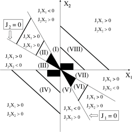
Let us identify the different modes of operation of the molecular motors on the diagram. The lines and are given by and , respectively. The slope of the line is higher than that of the line , i.e., because of the general condition that . The line divides the plane into two halves in one of which is positive while in the other is negative. Similarly also changes sign on crossing the line . In the regions II, IV, VI and VIII both the processes 1 and 2 are spontaneous and, consequently, energy is merely dissipated. In contrast, in the regions labelled by I, III, V and VII energy transduction take place; in I and V, the motor the process 2 drives the process 1 whereas in III and VII the process 1 drives the process 2.
8 Modeling stochastic chemo-mechanical kinetics: continuous landscapes vs. discrete networks
In general for modeling molecular motors four key choices need to be made [383]: (i) choice of the degrees of freedom, or dynamical variables, consistent with the intended level of spatio-temporal resolution, (ii) choice of the form of the interactions between the variables, (iii) choice of the dynamical equations depending on the nature of the dynamical variables, and (iv) choice of the methods of solution suitable for calculating the quantities of interest under the given initial and/or boundary conditions.
The hierarchy of the different levels of description used so far in modeling mechanics of molecular motors is shown in table 8 (MD molecular dynamics, NMA normal mode analysis).
Markov model: master equation for jump processes on “network” of states
Mechano-chemical model: Langevin/FP equation for BD on a “landscape”
Coarse-grained model: NMA for elastic “bead-spring networks”
Atomistic model: Classical MD; NMA of collective dynamics
In the following subsections, we mention a few alternative formalisms that model molecular motors at different levels of spatio-temporal resolution. We also explore the possible relations between them. Moreover, whereever possible, we mention a few alternative formalisms at the same level of spatio-temporal resolution and explain their relative advantages and disadvantages. In most of the approaches that we particularly emphasize below, we combine the fundamental principles of (stochastic) chemical kinetics with those of structural (Brownian) dynamics to formulate the general theoretical framework of mechano-chemistry or chemo-mechanics. The generic models of molecular motors as well as those for specific examples, which we review in the subsequent sections, are based on these formalisms.
8.1 Fully atomistic model, limitations of MD and normal mode analysis
Since we are interested neither in the making or breaking of covalent bonds nor in the very fast processes governed by quantum dynamics, solving time-dependent Schrödinger equation is not required. Therefore, in principle, classical molecular dynamins would be ideally suited to model the mechano-chemical dynamics of molecular motors. Unfortunately, in practice, the relevant time scales for the kinetics of molecular motors are too long to be accessed by MD simulation of fully atomistic models with the currently available computational resources. But, conceptually dividing these processes into shorter sub-processes, it has been possible to study the sub-processes independently by carrying out MD simulations of the corresponding atomistic models [384, 385].
However, some insight into the conformational dynamics of the motor can be gained by carying out the standard normal mode analysis (NMA) [386] of a fully atomistic model. The key idea behind NMA is the diagonalization of the Hessian matrix whose elements are the second derivatives of the potential energy in the harmonic appoximation. Obviously, starting with the fully atomistic force fields, the minimum energy configuration has to be found before studying the collective dynamics about such a configuration. The spectrum of the normal modes of these collective dynamics can be obtained numerically provided the Hessian matrix can be diagonalized using an efficient algorithm where is the number of atoms. In practice, huge computational resources are required for the energy minimization and the Hessian diagonalization for such fully atomistic models because is quite large for all molecular motors.
Because of the technical difficulties in structural measurements based on X-ray crystallography, high-resolution atomic structures of many motors are yet to be determined. Instead, structural information at lower resolution are often available from other probes, e.g., cryo-electron microscopy. Therefore, it is desirable to follow modeling strategy for which the low-resolution strutural information and limited computational resources are adequate to study the key dynamical processes theoretically. We discuss such modeling strategies in the next few subsections.
8.2 Coarse-grained model, elastic networks and normal mode analysis
If one is interested in developing a “structural” model that captures the intra-motor movements and conformational changes of the motor in each cycle, then the most convenient approximation would be a coarse-grained description [387, 388, 389, 390, 391]. Usually, a group of atoms is clustered together to be represented as a “site”, or “point particle”, of the coarse-grained model [391]. These “sites” are assumed to interact through an appropriate effective potentials. Such a coarse-grained model can be formulated, for example, by assigning a “point mass” (a bead) to each amino acid and postulating that these beads are connected by harmonic springs [392]. A more detailed model can be developed by assigning more than one bead per amino acid [388].
Insight into the actual kinetics of the motor can be gained by carrying normal mode analysis (NMA) which yields the spectrum of collective modes of the elastic network [393, 394, 395, 396, 397, 398, 399, 400]. A class of arbitrary deviations of the network from equilibrium, caused by small displacement of the individual bead positions, can be expressed as a linear combination of the normal modes [400].
The advantages and the limitations of this approach has been reviewed [401, 402]. From a theorists perspective, one of the limitations of the coarse-grained models is that even the minimal version is too complex to be treated analytically; only numerical results can be obtained. Even with the numerical techniques, in the absence of additional experimental information, it is very difficult to identify unambiguously which of the normal modes is functionally relevant for the given motor. Moreover, NMA considers small excursions from equilibrium whereas the deviations are quite large in many biological processes [400]. Nonlinear elastic effects, which are important for situations far from equilibrium, can be treated within the general framework of conformational relaxation of an elastic network [404]. Obviously, NMA is not a suitable technique for studying those dynamical features of the system that involve low degree of collectivity [403].
Coarse-grained approach cannot resolve chemical details, e.g., ATP-binding and hydrolysis. The effect of ATP binding is mimicked by establishment of new elastic links between the ATP-binding region of the motor and the coarse-grained domain where the ATP-binding site is located. Release of ADP and Pi is captured by the breaking of these elastic links. The free energy change caused by the hydrolysis is implicitly incorporated by the relaxation of the elastic strain following elastic link formation and breaking. Clearly, such descriptions of ATP binding and hydrolysis are not suitable for elucidating how the ATPase activity of a motor is coupled to its mechanical movement.
8.3 Stochastic mechano-chemical model: wandering on landscapes
The collective oscillations are expected to be strongly damped by the surrounding aqueous medium. Interactions of the motor with this aqueous medium, including the effects of thermal fluctuations, can be captured within the framework of coarse-grained models discussed in the preceeding subsection provided appropriate effective interactions between the elastic network and a coarse-grained representation of the aqueous medium can be prescribed [405]. In this subsection, we discuss an alternative approach that captures the effects of the aqueous medium indirectly in way that is standard practice in non-equilibrium statistical mechanics. Moreover, the coarse-grained models of this type involve far fewer dynamical variables and are capable to capturing non-collective dynamical features.
8.3.1 Motor kinetics as wandering in a time-independent mechano-chemical free-energy landscape
This formulation is useful for an intuitive physical explanation of the coupled mechano-chemical kinetics of molecular motors [406].
Being a protein or a macromolecular complex, a motor has a large number of degrees of freedom. At the microscopic level, a conformation of a motor is described by specifying the positions of all the constituent atoms in the 3-dimensional space. In the coarse-grained description that we discuss in this subsubsection, we retain only a few variables that are required for describing the most important dynamical processes of the motor on the relatively long relevant time scales. The remaining degrees of freedom are assumed to equilibrate so rapidly that they are treated as part of the reservoir that also includes the degrees of freedom associated with the surrounding aqueous medium.
Suppose is the full potential that depends on all the microscopic degrees of freedom. Based on the assumption mentioned above, the free energy of the motor (also called the potential of mean force) in the reduced -dimensional state space spanned by is obtained from
| (116) |
The potential gets contribution from (i) intra-motor interactions and interaction of the motor with its track, (ii) interaction of the motor with the fuel molecule, and (iii) interactions of the motor, track and fuel molecules with the molecules of the surrounding aqueous medium [407, 409].
Let us now divide the dynamical variables into two clases: “mechanical” variables and “chemical” variables , where . At least one of the variables must be “mechanical” variable that gives the position of the motor. For a porter on a linear track, the position is its actual location on the track. In case of a rotary motor, the position variable is actually an angle. Thus the “mechanical velocity” in this case would be either the linear or the angular velocity of the motor in real space. Additional mechanical variables may be used to denote, for example, the angle between two subunits of the motor, angles made by each of the subunits with the track, etc. Similarly, at least one of the variables must be a “chemical” variable that accounts for the progress of the chemical reaction which supplies the chemical input energy of the motor. In this case, the “chemical velocity” corresponds to the rate of the chemical reaction. For a motor driven by an electro-chemical gradient the chemical variable, in principle, can be redefined accordingly.
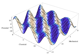
(a)
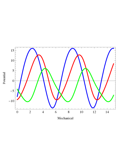
(b)
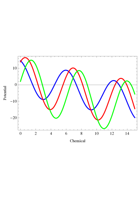
For the minimal case with a single mechanical variable and a single chemical variable the state space is essentially a 2-dimensional “land”, as shown schematically in fig16. Suppose and denote the mechanical and chemical variables, respectively. Then, the potential can be represented by the “height” at each point on the “land”. Since a track has equi-spaced binding sites for the motor, a cross-section of this landscape parallel to (i.e., for =constant) is periodic (see fig.17); all the local minima are equally deep and coincide with the location of the motor-binding sites on the track. On the other hand, as shown in fig.17, a cross-section of this landscape parallel to (i.e., for =constant) looks like a typical free energy diagram for a chemical reaction plotted against the reaction coordinate- two local minima, that correspond to the reactants and products, are separated by a free energy barrier. Since a molecular motor is a cyclic machine, the local minima parallel to also exhibit periodicity, except that the profile is tilted forward along the chemical direction, i.e.,
| (117) |
where is a constant and is the periodicity along . Because of the forward tilt of the profile along the bottom of the successive minima are deeper by which accounts for the lowering of free energy caused, for example, by ATP hydrolysis.
Using this scenario, Magnasco [408] argued how a coupling between the mechanical and chemical cycles in this space would give rise a chemically-driven mechanical motor. This would be the chemo-mechanical analog of the chemo-chemical machine of the kind that we discussed in section 6.
It is well known that for a classical system coupled to a reservoir, the deterministic time evolution of the system as well as the constituents of the reservoir is governed by a set of coupled Newton’s equations which exhibit the time-reversal symmetry. However, when the degrees of freedom associated with the reservoir are projected out, the dynamics of the system appears stochastic and irreversible; such time evolution of the system is described by a Langevin equation [410]. Therefore, in the minimal case of a 2-dimensional free-energy landscape, the Langevin equations are of the form
| (118) |
where and are the phenomenological damping coefficients for the mechanical and chemical variables, respectively; and are the corresponding external generalized forces, and being the corresponding generalized Brownian (noise) forces. Although the degrees of freedom associated with the reservoir do not appear as dynamical variables, their effects on the system enter the Langevin equation through the viscous damping term and random force term. Most often, for simplicity, the random generalized forces are assumed to be Gaussian white noise. The inertial terms have been neglected; this assumption is well justified for nano-motors whose motions are, in general, overdamped on the time scales relevant for motor movements.
An alternative, but equivalent, formulation is based on the Fokker-Planck equation [411] which, in the general case of -dimensional mechano-chemical state space, has the form
| (119) |
where is the probability that the motor protein is in the state at time . The two terms on the right hand side of eq.(119) account for the diffusion and drift of the motor in the free-energy landscape.
8.3.2 Motor kinetics as wandering in the time-dependent mechanical (real-space) free-energy landscape
In this subsection we consider those special situations where the chemical states of the motor are long lived and change in fast discrete jumps. Consequently, the mechanical variables of the motor can continue to change without alteration in its chemical states, except during chemical transitions when the mechanical variables remains frozen and at least one of the chemical variables changes abruptly. Because of this clear separation of the time scales of variation of the mechanical and chemical variables, no mixed mechano-chemical transition is allowed in this scenario.
In this formulation we assume that each of the mechanical variables is continuous whereas all the chemical variables are discrete. We now use the symbols and to denote the mechanical and chemical variables. As before, the free energy of the system is given by . Although, in principle, can be derived from the microscopic potential using eq.(116), in practice, its explicit form is most often postulated based on physical arguments.
The minimal model in this case also requires where the continuous variable denotes the position of the motor while the discrete variable () labels the chemical states. For example, if , the four distinct values of may correspond to the following chemical states of the motor: (a) ligand-free state, (b) ATP-bound state, (c) ADP-Pi-bound state, and (d) ADP-bound state. The free energy is plotted as a function of for a given discrete value of ; in general, different profiles correspond to different values of . A sequence of transitions of the chemical state is accompanied by the corresponding sequential change of the profile.
For the simplicity of explanation of this modeling strategy, let us consider the minimal case . In this case, the actual -dimensional potential landscape can be replaced by a sequence of one-dimensional potentials where is the number of discrete values allowed for the chemical state variable .
Because of the discrete nature of the chemical state variables, the eq.(119) is replaced by the equation
where is the transition probability per unit time for the transition from to while the mechanical variables remain frozen at the current instantaneous values; the symbol denotes values of all the chemical variables except the -th chemical variable. The condition of detailed balance imposes restrictions on the choice of these transition probabilities. Note that there is no term in this equation which would correspond to a mixed mechano-chemical transition.
Brownian ratchet
Let us assume the special values . Moreover, suppose , i.e., the chemical variable is allowed to take one of the only two allowed values so that only two different profiles of the free-energy landscape are possible. Let one of these be the flat form for all whereas the other be the sawtooth form shown in fig.18. Note the two key features of the sawtooth: (i) it is periodic, (ii) within each period, it has a spatial asymmetry.
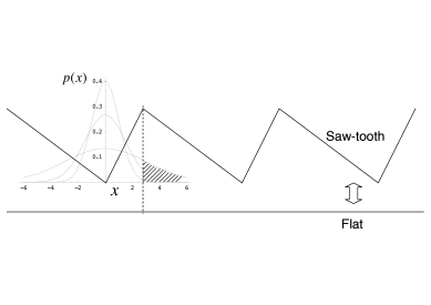
Suppose, initially the potential has the sawtooth shape and the motor is located at a point that corresponds to a minimum of the potential. As long as the potential remains unchanged, in spite of its spatial asymmetry, the average force on the motor (averaged over a single spatial period) because and . Thus, even if the motor position initially does not coincide with a minimum of the potential, given enough time, it will settle to the location of the nearest minimum of the free energy because of the energy dissipation by viscous drag against it. From then onwards, its position will exhibit only small amplitude thermal fluctuations around the potential minimum provided the thermal energy is much smaller compared to the height of the walls separating the successive wells of the potential profile. In addition, it will execute thermally-assisted occasional jumps to the neighboring wells symmetrically in both the forward and backward directions that, in the absence of any other processes, would result in only diffusion.
Let the chemical state of the motor make a transition to its other allowed state so that the potential profile makes a transition from its sawtooth form to its flat form. Immediately, the free particle begins to execute a Brownian motion and the corresponding Gaussian profile of the probability distribution begins to spread with the passage of time. If the potential is again switched on before the Gaussian profile gets enough time for spreading beyond the original well, the particle will return to its original initial position. But, if the period during which the potential remains off is sufficiently long, so that the Gaussian probability distribution has a non-vanishing tail overlapping with the neighboring well on the right side of the original well, then there is a small non-vanishing probability that the particle will move forward towards right by one period when the potential is switched on. Furthermore, the Gaussian profile may have a non-vanishing overlap with the well to the left of the original well that gives rise to the possibility of also moving backward in a cycle. But, because of the asymmetric shape of each period of the sawtooth, the overlap with the well on the right is larger than that with the well on the left; consequently, on the average, the particle would move to the right.
Thus, stochastic switching of the chemical variable back and forth between its two allowed discrete values can give rise to a “directed” movement of the motor, on the average, because of the asymmetric shape of each of the periods of the periodic sawtooth shaped potential profile. The resulting probability current is given by [414, 415]
| (121) |
with
| (122) |
where is the error function, the parameter is a measure of the spatial asymmetry of the sawtooth potential (symmetric sawtooth corresponds to ) and is the rate of flipping of the time-dependent potential.
Note that in this mechanism, the particle moves forward not because of any force imposed on it but because of its Brownian motion. The system is, however, not in equilibrium because energy is pumped into it during every period in switching the potential between the two forms. In other words, the system works as a rectifier where the Brownian motion, in principle, could have given rise to both forward and backward movements of the particle in the multiples of , but the backward motion of the particle is suppressed by a combination of (a) the time dependence and (b) spatial asymmetry of the potential. In fact, the direction of motion of the particle can be reversed by reversing the asymmetry in each period of the potential. The mechanism of directional movement discussed above is called a Brownian ratchet [418, 419, 420, 421, 422, 423, 424] The concept of Brownian ratchet was popularized by Feynman through his lectures [425] although, historically, it was introduced by Smoluchowski.
For a class of porters, for example, the switching of the chemical state is caused by ATP hydrolysis. The asymmetric periodic potential (whose shape is, at least qualitatively, somewhat similar to the sawtooth form) arises from the effect of the polarity of the filament on the motor-track interaction [412, 413]
The rectification of the noise required for Brownian ratchet mechanism can also be achieved by, for example, the binding of a ligand that stabilizes conformations in the “forward” direction [416]. This process has strong similarity with the conformational selection mechanism for substrate specificity of enzymes that we have discussed in section 6. The main difference between this mechanism of Brownian ratchet and the power stroke has been explained by Howard (see fig.1 of ref. [416]) with a simple illustration.
Efficiency of Brownian motors
Suppose, is the work done against a load force . The input energy for a Brownian motor can be calculated from
| (123) |
assuming a specific - and -dependence of the potential , where the angular bracket denotes average over many ratchet cycles. Hence the efficiency of a Brownian motor can be obtained from the definition
| (124) |
The directional movement of Brownian motors arises from the rectification of random thermal noise. For such motors, an alternative measure of performance is the rectification efficiency [426].
8.4 Markov model: motor kinetics as a jump process in a network of fully discrete mechano-chemical states
In this subsection we simplify the continuum landscape-based scenario developed in the preceeding subsection to formulate a fully discrete scheme making well-motivated approximations [406, 417]. With each local minimum of the free-energy landscape we associate a discrete state. The probability of finding the system in the -th discrete state is given by [406]
| (125) |
where -th zone is the immediate surrounding of the -th local minimum of the free energy landscape. Thus, the continuum of states is replaced by set of discrete states identified by the above procedure. Moreover, instead of the probability densities defined on the free energy landscape we now deal with the probabilities .
The local minima in the free-energy landscape are separated by low-energy passes so that thermal fluctuations occasionally cause the system to leave the neighbourhood of one local minimum and arrive at that of a neighboring one; such wanderings on the free energy landscape are identified as transitions from one discrete state to another in the fully discrete formulation. The corresponding rate constants (i.e., the probabilities of transition per unit time) can also be obtained from an analysis of the probability fluxes on the continuous landscape [406, 417]. Obviously, the rate constants depend on the shape of the free energy landscape; the dependence of the rate constants on the external force arise from that of the landscape shape on the external force.
The discrete state space of this formulation can be regarded as a network [427, 428, 429, 430]. Just like the continuum formulation, the minimal model must have one mechanical variable and a chemical variable both of which are discrete. Let be the probability of finding the motor at the discrete position labelled by and in the “chemical” state at time . Then, the master equation for is given by
| (126) | |||||
where the terms enclosed by the three different brackets correspond to the purely mechanical, purely chemical and mechano-chemical transitions, respectively. For obvious reasons, these equations are sometimes referred to as the stochastic rate equations.
As a concrete example, which will be used also for on several other occasions later in this review, consider a 2-state motor that, at any site , can exist in one of the only two possible chemical states labelled by the symbols and . We assume the mechano-chemical cycle of this motor to be
| (127) |
where the rates of the allowed transitions are shown explicitly above or below the corresponding arrow. Note that the transition is purely chemical whereas the transition is a mixed mechano-chemical transition. The corresponding master equations are given by
We’ll see some implications of these equations in several specific contexts later in this article.
Microscopic reversibility and balance conditions for mechano-chemical kinetics: cycles, and flux
The principle of microscopic reversibility [431] has important implications in the free energy transduction by molecular motors [432].
On a discrete mechano-chemical state space, each state is denoted by a vertex and the direct transition from one state (denoted by, say, the vertex ) to another (denoted by, say, the vertex ) is represented by a directed edge . The opposite transition from to is denoted by the directed edge . A transition flux can be defined along any edge of this diagram. The forward transition flux from the vertex to the vertex is given by while the reverse flux, i.e., transition flux from to is given by . Therefore, the net transition flux in the direction from the vertex to the vertex is given by .
A cycle in the kinetic diagram consists of at least three vertices. Each cycle can be decomposed into two directed cycles (or, dicycles) [433] where corresponds the clockwise and counter-clockwise cycles. The net cycle flux in the cycle , in the CW direction, is given by .
For each arbitrary dicycle , let us define the dicycle ratio
| (129) |
where the superscript on the product sign denote a product evaluated over the directed edges of the cycle. So, by definition, .
It has been proved rigorously [435] that, for detailed balance to hold, the necessary and sufficient condition to be satisfied by the transition probabilities is
| (130) |
For a non-equilibrium steady state (NESS), one can define [433] the dicycle frequency which is the number of dicycles completed per unit time in the NESS of the system. Then,
| (131) |
Clearly, , in general, for any NESS. There are close relations between this network formalism of energy transduction by molecular motors and a master equation based general network theory for microscopic dynamics [434] which is the microscopic counterpart of Kirchoff’s macroscopic theory of electrical networks.
Detailed balance is believed to be a property of systems in equilibrium whereas the conditions under which molecular motors operate are far from equilibrium. Does it imply that detailed balance breaks down for molecular motors? The correct answer this subtle question needs a careful analysis [436, 437, 438].
If one naively assumes that the entire system returns to its original initial state at the end of each cycle one would get the erroneous result that the detailed balance breaks down. But, strictly speaking, the free energy of the full system gets lowered by (e.g., because of the hydrolysis of ATP) in each cycle although the cyclic machine itself comes back to the same state. When the latter fact is incorporated correctly in the analysis [436, 437, 438], one finds that detailed balance is not violated by molecular motors. This should not sound surprising- the transition rates “do not know” whether or not the system has been driven out of equilibrium by pumping energy into it.
9 Solving forward problem by stochastic process modeling: from model to data
(a)

(b)

(c)

9.1 Average speed and load-velocity relation
For simplicity, let us consider the kinetic scheme shown in fig. (19(a)). In terms of the Fourier transform
| (132) |
of , the master equations can be written as a matrix equation
| (133) |
where is a column vector of components () and is the transition matrix in the -space (i.e., Fourier space). Other than the rate constants, also involves the -dependent factors
| (134) |
Summing over the hidden chemical states, we get the position probability density
| (135) |
Taking derivatives of both sides of (135) with respect to we get [440, 441]
where . Evaluating , in principle, the stationary drift velocity (i.e., asymptotic mean velocity) and the corresponsding diffusion constant can be obtained from
It may be tempting to attempt a direct utilization of the general form
| (138) |
where the coefficients are fixed by the initial conditions and are the eigenvalues of . However, for the practical implementation of this method analytically the main hurdle would be to get all the eigenvalues of . Fortunately, only the smallest eigenvalue , which dominates in the limit , is required for evaluating and [440, 441]:
| (139) |
Even the forms (139) are not convenient for evaluating and . Most convenient approach is based on the characteristic polynomial associated with the matrix , i.e., . Therefore, is a root of the polynomial , i.e., solution of the equation
| (140) |
| (141) |
where .
For a postulated kinetic scheme, is given. Then the expressions (141) are adequate for analytical derivation of and for the given model. However, in order to calculate the distributions of the dwell times of the motors, it is more convenient to work with the Fourier-Laplace transform, rather than the Fourier transform, of the probability densities. Therefore, we now derive alternative expressions for and in terms of the full Fourier-Laplace transform of the probability density.
Taking Laplace transform of (132) with respect to time
| (142) |
and inverting the matrix form of the master equation leads to the solution
| (143) |
where
| (144) |
and is the column vector of initial probability densities.
Applying the defnition of inverse of a matrix to the matrix R expressed in eqn.(144), the eqn.(143) takes the form
| (145) |
where are the cofactors of the R(k,s).
Now the determinant of , i.e., the characteristic polynomial has the general form which can be expressed as [439]
| (146) |
where, for reasons that will be clear as we proceed, the coefficients for only the three lowest order terms will be relevant for calculating the quantities of our interest.
9.2 Beyond average: dwell time distribution (DTD)
Two motors with identical average velocities may exhibits widely different types of fluctuations. Suppose the successive mechanical steps are taken by the motor at times . Then, the time of dwell before the -th step is defined by . In between successive steps, the motor may visit several “chemical” states and each state may be visited more than once. But, the purely chemical transitions would not be visible in a mechanical experimental set up that records only its position. The number of visits to a given state and the duration of stay in a state in a given visit are random quantities.
In order to appreciate the origin of the fluctuations in the dwell times, let us consider the simple -step kinetics:
| (148) |
Suppose is the duration of stay of the motor in the -th state during its -th visit to this state. If is the dwell time, then
| (149) |
where is the number of visits to the -th state. It is straightforward to check that
where is the average number of visits to the -th state and is the average time of dwell in the -th state is a single visit to it. More interestingly [309],
The first and second terms on the right hand side of (LABEL:eq-correl) capture, respectively, the fluctuations in the lifetimes of the individual states and that in the number of visits to a kinetic state. Note that the number of visits to a particular state depends on the number of visits to the neighboring states on the kinetic diagram; this interstate correlation is captured by the third term on the right hand side of (LABEL:eq-correl).
Several different analytical and numerical techniques have been developed for calculation of the dwell time distribution [442, 443, 444, 439]. Since the dwell time is essentially a first passage time [445], an absorbing boundary method [443] has been used.
An example: DTD for an irreversible motor with linear chain of ststes
As an example, we consider again the simple scheme (127). In this case, the DTD is
| (152) |
where
| (153) |
In the special case , and and, hence,
| (154) |
Similar sum of exponentials for DTD have been derived also for machines with more complex mechano-chemical kinetics (see, for example, refs.[446, 447, 448]).
9.2.1 A matrix-based formalism for the DTD
The matrix-based formalism that we have discussed above [439], for the calculation of and , has been extended to formulate general prescriptions for calculating the dwell time distribution . Let the Laplace transform of the DTD be denoted by . The general strategy, developed by Chemla et al.[439], for the calculation of is based three main steps: (i) obtaining by solving the master equation for in the Fourier-Laplace space; (ii) deriving a relation between and and using it, together with the solution obtained in step (i), to get ; and (iii) obtaining either from by inverse Laplace transform or, extracting at least the first few moments of from .
DTD for a motor that never steps backward
We now illustrate the method with the simple example
| (155) |
where the integer subscripts and label the discrete positions and of the motor on its track. The total number of “chemical” states of a motor at each position is . Note that the “chemical” transitions are reversible, but the “mechanical step” is irreversible; the latter rules out any possibility of backward stepping of the motor.
Suppose the initial condition is , i.e., the motor is certainly in the chemical state 1 at . For the kinetic scheme (155) under this initial condition, eqn.(145) becomes
| (156) |
Moreover, in this case, the relation between and is [439]
| (157) |
Equating the right hand sides of the eqns.(156) and (157), we get
| (158) |
DTD for a motor that steps both forward and backward
If and are the numbers of forward and backward steps, respectively, then for large , the corresponding step splitting probabilities are and . The dwell times before a forward step and before a backward step can be measured separately. Hence, the prior dwell times and can be obtained by restricting the summations in
| (159) |
to just forward (+) or just backward (-) steps, respectively. In terms of splitting probabilities and prior dwell times, the mean dwell time can be expressed as
| (160) |
Compared to the prior dwell times, more detailed information on the stepping statistics is contained in the four conditional dwell times, which are defined as follows:
It is helpful to introduce pairwise step probabilities . Note that , and . Neglecting finite time corrections,
Hence
| (163) |
Defining the post dwell times in a fashion similar to that used for defining the prior dwell times, we get
| (164) |
and
| (165) |
For motors which can step both forward and backward, more relevant information on the kinetics of a motor are contained in the conditional dwell time distributions [449, 439]. We illustrate the concepts and the matrix-based formalisms for such motors with the simple linear chain of states where all the transitions, including the mechanical transition, are reversible.
| (166) |
We define the conditional branching probabilities as the probability of taking a forward (+) or backward (-) step, given the previous step being forward (+) or bakward (-). Similarly, instead of one single DTD , we now have four conditional dwell time distributions (cDTD) . For convenience of calculation, we define the matrix
| (167) |
the diagonal matrix
| (168) |
and the column vector
| (169) |
In this case the relation between and the cDTDs is [439]
| (170) |
where is the vector of initial conditions. For example, corresponds to the given condition that the motor has taken the initial step in the forward (+) direction.
Extracting the cDTDs exploiting the relation (170) and the solution for is more complicated than the procedure we followed in the case of a single DTD. Let us begin with the case (i.e., given initial forward stepping) and the initial condition . For this case [439]
| (171) |
Equation (171) can be re expressed as
| (172) |
where
| (173) |
Hence,
| (174) |
and
| (175) |
Next we need to obtain directly from (145) and, by comparing it with eqn.(172), find out the expressions for and ; substituting these expressions for and into equations (174) and (175) we get and , respectively.
Similarly, for the case (i.e., given initial backward stepping) and the initial condition , one can derive the relation between and and . Obtaining the solution directly from (145) and, by utilizing its relation with and we can get the cDTDs in the Laplace space.
9.2.2 Extracting kinetic information from DTD
It is possible to establish on general grounds that, for a motor with mechano-chemical kinetic states like (148), the DTD is a sum of exponentials of the form [309]
| (176) |
where of the coefficients () are independent of each other because of the constraint imposed by the normalization condition for the distribution . Also note that the prefactors can be both positive or negative while for all .
Recall that for the Gamma distribution, the randomness parameter . Can the experimentally measured DTD be used to determine the number of states ? Unfortunately, for real motors, (i) not each step of a cycle is fully irreversible, (ii) the rate constants for different steps are not necessarily identical, (iii) branched pathways are quite common. Consequently, may provide just a bound on the rough estimate of .
Can one use the general form (176) of DTD to extract all the rate constants for the kinetic model by fitting it with the experimentally measured DTD? The answer is: NO. First, even if a good estimate of is available, the number of parameters that can be extracted by fitting the experimental DTD data to (176) is ( values of and values of ). On the other hand, the number of possible rate constants may be much higher [309]. For example, if transitions from every kinetic state to every other kinetic state is allowed, the total number of rate constants would be . In other words, in general, the kinetic rate constants are underspecified by the DTD. Second, as the expression (152) for the DTD of the example (127) shows explicitly, the ’s that appear in the exponentials may be combinations of the rate constants for the distinct transitions in the kinetic model. It is practically impossible to extract the individual rate constants from the estimated ’s unless any explicit relation like (153) between the estimated ’s and actual rate constants is apriori available.
The systematic method for extracting all the kinetic informations from experimental data are described in the next section where the utility of the DTD will be shown again.
10 Solving inverse problem by probabilistic reverse engineering: from data to model
A discrete kinetic model of a molecular motor can be regarded as a network where each node represents a distinct mechano-chemical state. The directed links denote the allowed transitions. Therefore, such a model is unambiguously specified in terms of the following parameters: (i) the total number of the nodes, (ii) the matrix whose elements are the rates of the transitions among these states; a vanishing rate indicates a forbidden direct transition.
In the preceding sections we handled the “forward problem” by starting with a model assuming the structure of the network and the transition rates. In this section we discuss the inverse problem for molecular motors after introducing the methodology. In most real situations the numerical values of the rate constants of the kinetic model are not known apriori. In principle, these can be extracted by analyzing the experimental data in the light of the model.
10.1 Frequentist versus Bayesian approach
Suppose, be a column vector whose components are the parameters of the model, i.e., the transpose of is Let the data obtained in observations of this model are represented by the -component column vector whose transpose is . Our “inverse problem” is to infer information on from the observed . The philosophy underlying the frequentist approach, i.e., approaches based on maximum-likelihood (ML) estimation and the Bayesian approach for extracting these information are different in spirit, as we explain in the next two subsubsections [450].
For simplicity, let us assume that a device has only two possible distinct states denoted by and .
| (177) |
Let us imagine that we are given the actual sequence of the states, over the time interval , generated by the Markovian kinetics of the device. But, the magnitudes of the rate constants and are not supplied. We’ll now formulate a method, based on ML analysis [451] to extract the numerical values of the parameters and .
Suppose and denote the time interval of the -th residence of the device in states and , respectively. Moreover, suppose that the device makes and visits to the states and , respectively, and is the total number of states in the sequence. Therefore, total time of dwell in the two states are and where .
Since the dwell times are exponentially distributed for a Poisson process, the likelihood of any state trajectory is the conditional probability density
| (178) | |||||
10.1.1 Maximum-likelihood estimate
ML approach [452] is based on finding the estimates of the set of model parameters that corresponds to the maximum of the likelihood for a fixed set of data . For the kinetic scheme shown in equation (177), the the ML estimates of and are obtained by using (178) in . It is straightforward to see [451] that these estimates are and .
10.1.2 Bayesian estimate
For drawing statistical inference regarding a kinetic model, the Bayesian approach has gained increasing popularity in recent years [453, 454, 455, 456, 457, 458]. The areas of research where this has been applied successfully include various biological processes in, for example, genetics [459, 460], biochemistry [461], cognitive sciences [462], ecology [463], etc.
In the Bayesian method there is no logical distinction between the model parameters and the experimental data; in fact, both are regarded as random. The only distinction between these two types of random variables is that the data are observed variables whereas the model parameters are unobserved. The problem is to estimate the probability distribution of the model parameters from the distributions of the observed data.
The Bayes theorem states that
| (179) |
where can be expressed as
| (180) |
The likelihood is the conditional probability for the observed data, given a set of particular values of the model parameters, that is predicted by the kinetic model. However, implementation of this scheme also requires as input. In Bayesian terminology is called the prior because this probability is assumed apriori by the analyzer before the outcomes of the experiments have been analyzed. In contrast, the left hand side of equation (179) gives the posterior probability, i.e., after analyzing the data.
Thus, an experimenter learns from the Bayesian analysis of the data. Such a learning begins with an input in the form of a prior probability; the choice of the prior can be based on physical intuition, or general arguments based, for example, on symmetries. Prior choice can become simple if some experience have been gained from previous measurements. Often an uniform distribution of the model parameter(s) is assumed over its allowed range if no additional information is available to bias its choice. To summarize, Bayesian analysis needs not just the likelihood but also the prior .
For the kinetic scheme shown in equation (177), the Bayes’ theorem (179) takes the form
| (181) | |||||
We now assume a uniform prior, i.e., constant for positive and , but zero otherwise. Then, is proportional to the likelihood function (within a normalization factor). Normalizing, we get
| (182) |
The mean of obtained from the posterior distribution is whereas the corresponding ML estimate is . Similarly, the mean obtained from the posterior distribution and the ML estimate of are obtained by replacing the subscripts by subscripts . Moreover, the variance of and calculated from the posterior distribution are and , respectively.
10.2 Hidden Markov Models
The actual sequence of states of the motor, generated by the underlying Markovian kinetics, is not directly visible. For example, a sequence of states that differ “chemically” but not mechanically do not appear as distinct on the recording of the position of the motor in a single motor experiment. This problem is similar to an older problem in cell biology: ion-channel kinetics [464, 465]. Current passes through the channel only when it is in the “open” state. However, if the channel has more than one distinct closed states, the recordings of the current reveals neither the actual closed state in which the channel was nor the transitions between those closed states when no current was recorded.
Hidden Markov Model (HMM) [466, 467, 468, 469, 470] has been applied to analyze FRET trajectories [471, 472], stepping recordings of molecular motors [473, 474], and actomyosin contractile system [475] to extract kinetic information.
For a pedagogical presentation of the main ideas behind HMM, we start with the kinetic scheme shown in (179) and a simple, albeit unrealistic, situation and then by gradually adding more and more realistic features, explain the main concepts in a transparent manner [451]. First, suppose that the actual sequence of states (trajectory) itself is visible; this case can be analyzed either by the ML-analysis of by Bayesian approach both of which we have presented above. We now relax the strong assumption about the trajectory and proceed as below.
If state trajectory is hidden and visible trajectory is noise-free
The sequence of states of the device is, as before, generated by a Markov processes which is hidden. Suppose the device emits photons from time to time that are detected by appropriate photo-detectors. For simplicity, we assume just two detection channels labelled by and . For the time being, we also assume a perfect one-to-one correspondence between the state of the light emitting device and the channel that detects the photon. If the channel () clicks then the light emitting device was in the state () at the time of emission. The interval between the arrival of the -th and -th photons () is random.
Thus, from the photo-detectors we get a visible sequence of the channel index (a sequence made of a binary alphabet) which we call “noiseless photon trajectory” [451]. The sequence of states in the noiseless photo trajectory is also another Markov chain that is conventionally referred to as the “random telegraph process”. Note that the photon detected by channel 1 (or, channel 2) can take place at any instant during the dwell of the device in state 1 (or, state 2). Therefore, the sequence of states in the noiseless photon trajectory does not reveal the actual instants of transition from one state of the device to another.
Since the noiseless phton trajectory corresponds to a random telegraph process, the transition probabilities for this process are
where is the conditional probability that state of the device is given that it was in the state at a time earlier.
The likelihood of the visible data sequence is now given by
| (184) |
where the first factor on the right hand side is the initial probability (usually assumed to be the equilibrium probability). The transition probabilities on the right hand side of equation (184) are the conditional probabilities given in equation (LABEL:eq-condprob). Unlike the previous simpler case, where the state sequence itself was visible, no analytical closed-form solution is possible in this case. Nevertheless, analysis can be carried out numerically.
If state trajectory is hidden and visible trajectory is noisy
In the preceeding case of a noise-free photon trajectory, we assumed that from the channel index we could get perfect knowledge of the state of the emitting device. More precisely, the conditional probabilities were
| (185) | |||||
However, in reality, background noise is unavoidable. Therefore, if a photon is detected by the channel , it could have been emitted by the device in its state (i.e., it is, indeed, a signal photon) or it could have come from the background (i.e., it is a noise photon). Suppose is the probability that the detected photon is really a signal that has come from the emitting device. Suppose is the probability of arrival of a background photon in the channel 1. The probability that a background photon arrives in channel 2 is . Then [451],
Thus, in this case, the relation between the states of the hidden and visible states is not one-to-one, but one-to-many.Therefore, given a hidden state of the device, a set of “emission probabilities” determine the probability of each possible observable state; these are listed in equations (LABEL:eq-emissionprob2) for the device (177).
10.2.1 HMM: formulation for a generic model of molecular motor
On the basis of the simple example of a 2-state system presented above,
we conclude that, for data analysis based on a HMM four key ingredients
have to be specified:
(i) the alphabet of the “visible” sequence (),
i.e., possible distinct visible states;
(ii) the alphabet of the “hidden” Markov sequence
(), i.e., allowed distinct hidden states,
(iii) the hidden-to-hidden transition probabilities , and
(iv) hidden-to-visible emission probabilities .
In addition to the transition probabilities and emission probabilities,
which are the parameters of the model, the HMM also needs the initial
state of the hidden variable(s) as input parameters.
Visible: V0 V1 … Vt VT
Hidden: H0 H1 … Ht HT
Suppose denotes the probability that an HMM with parameters generates a visible sequence . Then,
| (187) |
where is the conditional probability that the HMM generates a hidden sequence for the given parameters and is the conditional probability that, given the hidden sequence (for parameters ) the visible sequence would be obtained.
Once is computed, the parameter set are varied to maximize (for the convenience of numerical computation, often ln is maximized. The total number of possible hidden sequences of length is . In order to carry out the summation in equation (187) one has to enumerate all possible hidden sequences and the corresponding probabilities of occurrences. A successful implementation of the HMM requires use of an efficient numerical algorithm; the Viterbi algorithm [476, 477] is one such candidate.
In case of a molecular motor, the “chemical states” are not visible in a single molecule experiment. Moreover, even its mechanical state that is “visible” in the recordings may not be its true position because of (a) measurement noise, and (b) steps missed by the detector. Let us denote the “visible” sequence by the recorded positions whereas the hidden sequence is the composite mechano-chemical states where and denote the true position and chemical state, respectively. The transition probabilities are denoted by One possible choice for the emission probabilities is [473]
| (188) |
In this case,
| (189) |
where
| (190) |
and
| (191) |
The usual strategy [471, 473] consists of the following steps: Step I: Initialization of the parameter values for iteration. Step II: Iterative re-estimation of parameters for maximum likelihood: the parameters , and are re-estimated iteratively till saturates to a maximum.
Step III: Construction of “idealized” trace: using the final estimation of the model parameters, the position of the motor as a function of time is reconstructed; naturally, this trace is noise-free.
Step IV: Extraction of the distributions of step sizes and dwell times: the distributions of the steps sizes and dwell times are obtained by constructing the distributions of the vertical and horizontal segments, respectively, of the idealized trace. These distributions can be compared with the corresponding theoretical predictions.
The strategy developed above turns out to be very successful in extracting the parameters for a well-defined model. However, in the case of specific molecular motors, not only the rate constants but also the number of states and the overall architecture of the mechano-chemical network as well as the kinetic scheme postulated by the model may be uncertain. In that case, the experimental data should be utilized to “select” the most appropriate model from among the plausible ones. In fact, more than one model, based on different hypotheses, may appear to be consistent with the same set of experimental data within a level of accuracy. The experimental data can be exploited at least to “rank” the models in the order of their success in accounting for the same data set. Unfortunately, as we’ll summarize later in this review, very little effort has been made so far in this direction for inferring and ranking models of molecular motors based on empirical data.
11 Motoring along filamentous tracks: generic models of porters
So far as intracellular transport is concerned, the two basic mechanisms are: (i) passive diffusion, and (ii) active transport driven by molecular motors. Stochastic models of these two processes have been reviewed very recently from the perspective of applied mathematicians [478]. Here we focus on the molecular motors and motor-driven active processes from the perspective of statistical physicists. The generic models ignore the details of the composition and structure of the track as well as those of the architectural design of the motors.
11.1 Phenomenological linear response theory and modes of operation
We identify the external load force opposing the movement of the motor and the chemical potential difference as the two generalized forces and . The corresponding generalized fluxes and are, respectively, the average spatial velocity of the motor and the average rate of ATP hydrolysis, measured in terms of the average number of ATP molecules hydrolyzed per unit time [372]. The modes of operation on the plane is identical to the generic ones sketched on the plane in fig.15.

Figure NOT displayed for copyright reasons.
The above scenario is deterministic and holds only in the linear response regime. In order to go beyond [479, 480], let us consider the concrete case of cytoskeletal motors. A motor can step forward () or backward () both by hydrolyzing one molecule of ATP (see fig.20). The corresponding reverse processes ( and ) synthesize one molecule of ATP. The process and the corresponding reverse process are purely mechanical processes which do not change the number of ATP molecules. Similarly, and are purely chemical processes which do not change the position of the motor. Let the instantaneous state of the system at any arbitrary instant of time be denoted by the position of the motor and the number of ATP molecules (see fig.20). The symbols denote the probabilities of the respective processes defined above. These probabilities must satisfy the relations [479, 480]
| (192) |
where is the step size of the motor. If is the time of a cycle, the velocity of the motor is then given by
| (193) |
Hence, rearragning the terms, and using (192), we get [480]
| (194) |
Similarly, the reaction rate is given by [480]
| (195) |
Using the equations (194) and (195), instead of linear response relations between and , the modes of operation of the molecular motor in this scenario can be analyzed. The resulting modes and the corresponding sectors on the space are shown in fig.21. A similar analysis was reported also by Liepelt and Lipowsky [481].
However, it has been argued [433] that, for motors at a fixed temperature and driven by ATP hydrolysis, the 2-dimensional space spanned by the load force and the chemical potential diference is only a sub-space of the full 4-dimensional space spanned by , , and .
Thermal reservoir () Work reservoir ()
Molecular motor
ATP reservoir () ADP reservoir () P reservoir ()
11.2 A generic model of a motor: kinetics on a discrete mechano-chemical network
To my knowledge, a generic 3-state stochastic model, with unbranched cyclic kinetics, was proposed first by Qian [482, 483] for the mechano-chemistry of molecular motors. As an illustrative example, let us consider the unbranched mechano-chemical cycle [26] with , as shown in fig.23. This special value of is motivated by the typical example of a kinesin motor for which the four essential steps in each cycle are as follows: (i) a substrate-binding step (e.g., binding of an ATP molecule), (ii) a chemical reaction step (e.g., hydrolysis of ATP), (iii) a product-release step (e.g., release of ADP), and (iv) a mechanical step (e.g., power stroke).

Suppose, The forward transitions take place at rates whereas the backward transitions occur with the rates . The average velocity of the motor is given by [26]
| (196) |
where
| (197) |
with
| (198) |
while is given by
| (199) |
where
| (200) |
and
| (201) |
while,
| (202) |
For various extensions of this scheme see ref.[26].
In the simpler case shown in (127), where , and the second step is purely irreversible, using the step size explicitly (to make the dimensions of the expressions explicitly clear), we get
| (203) |
Note that if, in addition, vanishes, i.e., if both the steps are fully irreversible, then , i.e., the average time taken to move forward by one site is the sum of the mean residence time in the two steps of the cycle.
11.3 2-headed motor: generic models of hand-over-hand and inchworm stepping patterns
The stepping pattern of a 2-headed motor can be either “hand-over-hand” or “inchworm” (see figs.24 and 25). In the HoH stepping pattern, each head alternates between leading and lagging position as the motor steps forward. In contrast, in the inchworm pattern, the leading head always leads while the lagging head always lags.
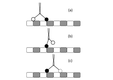
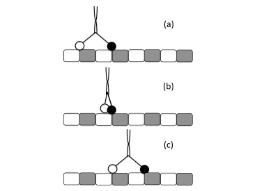
One of the approaches for modeling 2-headed motors is based on Brownian ratchets. In this approach one begins with two identical heads each of which, at least for part of each cycle, is subjected to a periodic potential which represents its interaction with the periodic track. Then the two heads are coupled by an elastic spring to construct a 2-headed motor. One writes Langevin equations for each head which are coupled because of the spring. In some models (see, for example, Dan et al.[484]) the potential seen by each head is time-dependent so that each head is effectively a flashing ratchet, e.g., potential switching alternately between a sawtooth () and a flat form (). The potential felt by the two heads are out of phase so that when one feels , the other feels and vice-versa (see ref.[485] for a slightly different formulation in terms of two sawtooth potentials that are shifted with respect to each other by half the spatial period). In an alternative formulation Derenyi and Vicsek [486] assumed the potential to be time-independent whereas the relaxed length of the spring was assumed to alternate between 0 and 8 nm in each cycle. Mogilner et al.[487] modelled a generic 2-headed motor where the conformational changes induced by ATP binding and/or hydrolysis gives rise to asymmetric internal velocity fluctuations. They showed that (noisy) directed motion of the motor is a consequence of the rectification of these velocity fluctuations by “protein friction” [488].
Kumar et al.[489] modeled the inchworm stepping of 2-headed motors by a generic Brownian “active elastic dimer”. In this model the two heads, whose positions are given by the coordinates are and , are coupled by a elastic spring. The damping coefficient of the heads are assumed to depend on the relative coordinate , i.e., on the elastic strain. The Langevin equation for the individual monomers include not only a strain-dependent damping, but also two noise terms one of which is thermal noise while the other is a non-equilibrium (or, active) noise. The model displays a counterintuitive reversal of the velocity of the center of mass with the variation of characteristics of damping. The key ingredient is the strain-dependent damping. As argued by the authors [489], the stretch-dependent damping in this model is “encoded” in the fact that the ATP-bound (free) first head encounters a higher (lower) barrier against motion than that faced by the second head.
Next we study a generic model for the hand-over-hand stepping pattern of a 2-headed motor. As before, the track is represented by a linear chain with equispaced binding sites that are labelled by the integer index ().
We first sketch the strategy adopted by Kolomeisky and Phillips [490] who extended the Fisher-Kolomeisky model [608, 26] described above. There are discrete biochemical states on the pathway in between two successive sites and . The separation between the successive binding sites is . In the HoH stepping pattern, the two heads are assumed to move alternately: the trailing head, labelled as , goes through transitions among the intermediate states while the other head, labelled as , remains anchored to its own position; in this process the head becomes the leading head and the head becomes the trailing head. Next, head remains static while head executes its transitions among its own intermediate states to regain its leading position ahead of head . Thus, in a single cycle each head moves ahead by a distance and, the center of mass moves forward by . Consequently, for the purpose of quantitative calculations, the overall translocation of the motor can be represented as a motion of two particles on two parallel periodic lattices; the distance between two neighboring sites on each lattice is . In this case, the average velocity and the diffusion constant are given by the expressions (203).
An alternative approach was developed earlier by Peskin and Oster [491]. The two heads of the motor are connected at a hinge. The angle made by the two heads at the hinge can increase up to a maximum that corresponds to the separation between the two heads. For simplicity, we assume that each head of the 2-headed motor can exist in one of the two allowed states which are designated as “strongly” attached state (labelled by index 1) and “weakly” attached (labelled by index 0) [491]. The transition corresponds to detachment of the head from the track whereas the next transition corresponds to its re-attachment.
When both the heads are attached to the track, the rates of detachment of the front head and that of the back head are denoted by the symbols and , respectively. If only one head is attached to the track, is the rate of reattachment of the unattached head. The unattached head attaches in front of the already attached head with probability (the unattached head attaches behind the already attached head with probability ). Since we are interested in the average velocity of the motors during a single run, both the heads can be detached only before, and after, each run. We now make the following assumptions [491]: (I) , and (II) .
The state of the motor, as a whole, is specified by specifying the corresponding states of the two heads. In principle, there are three state, namely (1,1), (1,0), (0,1) because, for reasons explained above, the state (0,0) is not allowed. We simply the description even further by noting that the states (1,0) and (0,1) describe the same state. Thus, the motor has two states, namely, (1,1) in which both the heads are attached and (1,0)=(0,1) in which only one head is attached while the other is detached. According our convention, the motor position is obtained by the following rule: if both the heads are attached then coincides with the mid-point which is also the position of the hinge. However, if only one head is attached, then is identified as the position of the bound head. Thus, can change by . Denoting the positions of the states (1,1) by integer index and those of the states (1,0)=(0,1) by half-integer indices , we can represent the hand-over-hand stepping pattern of the motor by the Markov chain shown in the fig.26.
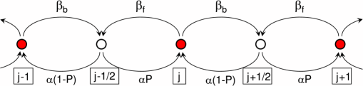
The probabilities that the motor position is and are denotes by and , respectively. The corresponding master equations are
| (204) |
We define the -th moments and . It follows from (204), in the steady state,
| (205) |
and the average velocity
| (206) |
where and . Note that the asymmetries of both detachment and reattachment inherent in the assumptions (I) and (II) give rise to the two positive terms within the square bracket of eqn.(206). This generic model of 2-headed motor assumes these asymmetries; we’ll explain the physical origin of such asymmetries of real two-headed motors when we study specific examples in part II of this review.
Traffic-like collective movement of motors: totally asymmetric simple exclusion process
So far we have discussed mostly a single isolated porter walking on its track. Now we present a generic model of traffic-like collective movements of many porters simultaneously on the same filamentous track. The model developed by Aghababaie et al.[492] for this purpose is based on an abstract formulation of Brownian ratchet. However, most of the subsequent works have been based on the asymmetric simple exclusion process (ASEP) [493].
An ASEP is a simple particle-hopping model where “particles” can hop, with some probability per unit time, from one lattice site to a neighboring site if, and only if, the target site is not already occupied by another “particle”. Thus, simultaneous occupation of any site by more than one particle is ruled out in this model; this fact is expressed by the term “simple exclusion”. The terms “asymmetric” expresses the fact that the particles have a preferred direction of motion. If the particles move only in one direction, and never in the opposite direction, the model is further specialized to totally asymmetric simple exclusion process (TASEP). In the general case, a particle hops forward with a rate if the target site is empty. So far as the kinetics is concerned, random sequential updating of the states of the system is implemented in discrete time steps. The number of particles passing through a given site per unit time is defined as the flux; in the steady state, because of the equation of continuity, the flux is independent of the lattice site.
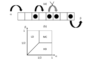
For a finite lattice boundary conditions have to be imposed. Although periodic boundary conditions are imposed often for the simplicity of calculation or as an intermediate step, the open boundary conditions capture the molecular motor traffic more realistically. In the latter case, particles enter from one end at a rate and exit from the opposite end at the rate . At any instant of time, the number density of the particles is defined by where is the total number of particles distributed over the lattice that consists of a total of sites. Obviously, under the periodic boundary conditions, is independent of time and the steady-state flux depends on and . The plot of against is called the fundamental diagram. As expected, at sufficiently low number density of the particles, the flux increases with , although the rate of increase decreases with increasing because of the stronger hindrance effects. After attaining a maximum at a certain density , the flux keeps decreasing with further increase of , eventually vanishing at . In contrast, under open boundary conditions, the number density fluctuates. This version of TASEP serves as the prototype for the non-equilibrium systems that exhibit boundary-induced phase transitions [494]. On a plane spanned by the parameters and , the system exhibits an interesting phase diagram [493]. The three phases are identified as (see fig.27) the (i) low-density (LD) phase, (ii) high-density (HD) phase, and (iii) maximal current (MC) phase; the rate limiting process for the three phases correspond to the rate constants , and respectively.
TASEP and its various extensions have been used extensively for modeling vehicular traffic and many similar systems [495, 496, 497]. In the context of molecular motors, the “particle” represents a motor while the lattice represents its track, the lattice sites being the binding sites for the motor. A one-dimensional TASEP is adequate for generic models of molecular motor traffic [498]. In the generic models of molecular motor traffic, one should also include the possibility of attachment of a motor at any vacant binding site and detachment from any occupied site of the lattice. Almost all the models of molecular motor traffic reported in the physics literature [499, 500, 501, 502, 503, 504, 505, 506, 507, 508, 509] are essentially extensions of TASEP that incorporates, in addition, a Langmuir-like kinetics of adsorption and desorption of the particles. Analyzing their model, Parmeggiani et al.[506] demonstrated a novel phase of the system in which the low- and high-desity regions, separated by a domain wall, co-exist [507, 508]. This spatial organization can be interpreted as a traffic jam of molecular motors.
12 Sliders and rowers: generic models of filament alignment, bundling and contractility
Flexible parallel filaments are known to form bundles in the presence of passive cross-linking molecules with two adhesive end groups [510]. Effects of cross-linking by active cross-linkers can be more dramatic. For example, molecular motors can align two filaments that are initially not parallel to each other; such “zipping” of two polar filaments is a cooperative effect of multiple motors [511, 512]. Alignment of more than two such filaments by the collective effort of multiple motors can lead to the formation of filament bundles. Suppose denotes the angle between the two polar filaments. Then, in the kinetic model of motor-induced alignments of these two filaments [512], the time-evolution of is described by a torque balance equation. Alignment of the two filaments involves not only rotation about the point of intersection of the two filaments, but also movement of the intersection point itself. Moreover, these two aspects of the dynamics are driven collectively by cross-linking molecular motors. Therefore, in addition to the equation for , a separate equation accounts for the movement of the point of intersection (crossing point) of the two filaments. Furthermore, these two equations are coupled to the appropriate equations for the stepping kinetics of the motors that describe their diffusion, drift as well as their attachment to and detachment from the filaments. The mean time needed for such motor-driven alignment of two polar filaments is at least an order of magnitude faster than that required for alignment by passive cross-linkers.
Continuum models for the generic situation of relative sliding of active filaments by active linkers were developed by Kruse, Jülicher and collaborators [513, 514, 515, 516]. Suppose and denote the number densities (i.e., number per unit length) of the filaments whose plus ends are oriented in the and directions, respectively. The total number density and the polarization density of the filaments are given by and , respectively. If all the filaments are oriented in the same direction, . The dynamics of the system is described by the two equations of continuity, with the respective source terms, and [516]
| (207) |
where the currents and arise from the change of relative positions and orientations of the filaments induced by the active cross linkers. These currents include, in addition to drift, also diffusion currents caused by the fluctuations in and . In the absence of polymerization and depolymerization of the filaments, . This model has been extended by Peter et al.[517] incorporating effects of its coupling to a visco-elastic network.
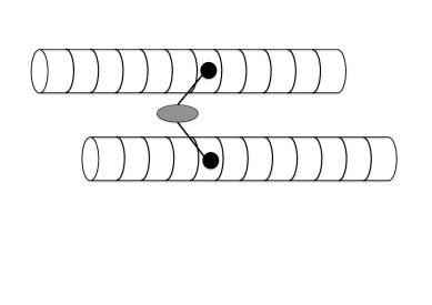
Kruse and Sekimoto [514] proposed a discrete model for motor-induced relative sliding of two filamentary motor tracks (see Fig.28). Each of the two-headed motors is assumed to consist of two particles that are connected to a common neck and are capable of binding with two filaments provided the two corresponding binding sites are closest neighbours. Each particle can move forward following a TASEP-like rule and every step of this type causes sliding of the two filaments by one single unit. The average relative velocity of the filaments was found to be a non-monotonic function of the concentration of the motors [514].
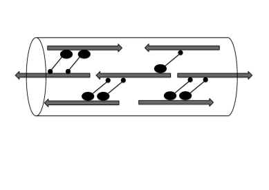
Zemel and Mogilner [141] studied a generic discrete model of motor-driven sliding and bundling of filaments by computer simulations (see fig.29). In this model the equation of motion of the -th filament is assumed to have the form (), where the actual form of the force depends on the force-velocity relations postulated for the filament-sliding motors. Suppose is the total number of potential crossbridges between pairs of filaments in the bundle. Then, is the fraction of active overlaps in the bundle if is the actual number of crossbridged formed by the sliding motors. and the number density of the motors (i.e., number of motors per unit length) bound to the filaments are the two important model parameters that, in turn, depend on the concentration of the motors. The model can simulate wide varieties of situations. For example, in general, a fraction of the filaments can have left-polarity while the remaining fraction has right-polarity. Both unipolar and bipolar sliding motors were modeled. Unipolar motors, which have motor domain at one end and the cargo-binding domain at the other, mimic kinesin-1 or cytoplasmic dynein. In contrast, bipolar motors have motor domains at both ends and mimic, for example, kinesin-5. Moreover, the results depend on the choice of the boundary conditions; both period and open boundary conditions were imposed in different sets of simulations. Although, for simplicity, it was formulated as a one-dimensional model, its simulation provided interesting insight into physics of filament sorting and pattern formation [141].
The Brownian ratchet mechanism of free energy transduction by molecular motors for sliding of filaments have been discussed in the literature for many years [518, 519, 520]. A Brownian ratchet model for the kinetics of “cross-bridge” of a single motor and a filament was developed by Cordova et al. [521]. It can also account for () cross-bridges formed by multiple motors simultaneously with the same filament. Physically motivated forms of the probabilities of attachment and detachment of the motors (i.e., probabilities for the formation and break-up of cross-bridges) were postulated. The sliding of the filament by the intact cross-bridges is taken into account by equating the velocity of the fiber with the collective velocity of the cross-bridges. The overdamped Langevin equation describing the one-dimensional dynamics of the filament includes not only the viscous drag and random Brownian force, but also the elastic restoring force of the stretched cross-bridge and the external load force. The force-velocity relation for this model can be obtained by solving this equation numerically.
13 Nano-pistons, nano-hooks and nano-springs: generic models
So far the cytoskeletal filaments have played a secondary role as tracks for the respective motors whose mechanisms of energy transduction and force generation were of primary interest to us. In this section we review the generic mechanisms of force generation by polymerizing and depolymerizing filaments which work, effectively, as nano-pistons and nano-hooks, respectively. Since the elastic stiffness of these filaments are crucial for force generation, a brief introduction to their elastic properties, particularly their stretching and bending stiffnesses, is given in the appendix J.
Operation as nano-piston and nano-hook are not the only possible modes of motor-independent force generation by filamentous polymers. Spring-like actions of filamentous structures are known to drive fast motility of some biological systems [146]. One well known example of such biological spring is the vorticellid spasmoneme whose major protein component is spasmin [522, 523]. The sperm cell of the horse-shoe crab Limulus polyphemus also utilizes the spring-like action of a coiled bundle, which consists mainly of actin filaments, to penetrate into an egg for its fertilization [524, 525]. The cytoskeleton of the red blood cell has also been proposed to be a form of active nano-spring [526]. However, in this review we’ll neither review these mechanisms nor the mechanisms of force generation by a jet of oozing gel through a nozzle [527, 528, 529, 530, 531, 532, 533] and that by shrinking gels resulting from crosslinking and bundling of filaments [534]. The effects of the distinct structural and kinetic features of the different types of polymerizing filaments on the force generation will be discussed in section 20.
13.1 Push of polymerization: generic model of a nano-piston
13.1.1 Phenomenological linear response theory for chemo-mechanical nano-piston: modes of operation
Suppose denotes the concentration of the monomeric subunits of the filamentous polymer in solution and denotes the load force. Then, and can be treated as the two relevant “generalized forces” for a phenomenological linear response theory for nano-pistons [535]. The possible modes of operation of the nano-piston and the corresponding parameters regimes on the 2d plane spanned by these two generalized forces [535] are shown schematically in fig.30.
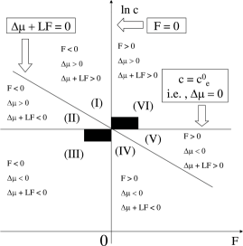
13.1.2 Stochastic kinetics of chemo-mechanical nano-piston
Suppose the rates of attachment (on-rate) and detachment (off-rate) of the tubulin dimers to the MT are denoted by and , respectively, in the absence of load force. Let be the free energy difference between the on and off states. Obviously, . However, in the presence of a load force opposing the filament growth, we get
| (208) |
based on purely thermodynamic arguments (see, for example, ref.[536]) where is the monomer length. Hence, the force-velocity relation for the nano-piston is given by
| (209) |
where the parameter accounts for the load distribution [540]. Therefore, the corresponding stall force is [538]
| (210) |
This final result is not surprising because the entire chemical free energy input is spent in stalling the nano-piston.
A statistical mechanical treatment that takes into account fluctuations, was formulated by Peskin et al.[538] in terms of a Fokker-Planck equation. Let us put the origin of the coordinate system on the tip of the polymerizing filament. We represent the position of the membrane by a “particle”; thus, the position of the particle () is also the gap between the tip of the MT and the membrane. We define the density such that is the number of filaments (in an ensemble) that has value lying between and at time . The FP equations for are [538]
where the concentration of dimers in the solution, and is the Heaviside step function. In the steady-state the force-velocity relation is obtained from
| (212) |
13.2 Pull of de-polymerization: generic model of a nano-hook
The force generated by a depolymerizing filament was originally developed in the context of chromosome segregation. Therefore, we defer a detailed discussion to the section 21. In this subsection we study force generation by depolymerizing filaments in a similar in-vitro experiment [539]. In this experiment a micron-size bead diffuses on a filament that is simultaneously depolymerizing.
The filament is represented by a one-dimensional lattice of lattice constant . The right end of the lattice corresponds to the depolymerizing tip. Therefore, the lattice shortens, from the right to left, by a length , at the rate per unit time. Unless located on the tip of the filament, the bead hops towards right and left with rates and , respectively, per unit time. When the bead is located exactly on the tip of the filament and hops to the left, it has a probability of “peeling off” the terminal subunit from the filament. Solving the kinetic equations in the steady-state, one gets the force-velocity relation [491]
| (213) |
where and .
14 Exporters and importers of macromolecules: generic models
The cell membrane separates the interior of the cell from its surroundings. It is essential for maintaining the integrity of the cell. At the same time, the cell cannot survive without exchange of matter and energy with its surroundings. Therefore, the cell membrane must be capable of performing a remarkable task: on the one hand, it must allow export/import of molecules across itself that are necessary for sustaining the life of the cell and, on the other, it should prevent all those transport processes which can threaten the survival of the cell. The same properties are also shared by internal membranes of eukaryotic cells which maintain the integrity of various compartments that perform specialized functions.
Macromolecules to be translocated across the pore may be hydrophobic or may be electrically charged. Therefore, it is not surprising if it encounters an energy barrier while trying to translocate across the pore. However, what makes macromolecule translocation even more interesting from statistical physics perspective is that the macromolecule also encounters an entropic barrier [541]. The number of allowed conformations of the macromolecular chain, and hence its entropy, is drastically reduced when it translocates across a narrow pore. Therefore, in general, the barrier encountered by the translocating macromolecular chain is a free energy barrier. Naturally, in order to overcome the free energy barrier against its passage across a membrane a macromolecule, in general, requires energy supply which is provided, most often, by the action of the corresponding translocation motor [542, 543].
In this section we review the generic models of “translocators” [544], i.e., motors that translocate linear polymers across a narrow passage on a surface. The process of macromolecule translocation can be divided into two steps. Step I: The tip of the macromolecule just enters the pore; step II: the entire length of the chain crosses the pore. The first process is analogous to putting the tip of a thread through the hole of a needle whereas the second is the analogue of pulling a length of that thread through the same hole after successful insertion of the tip. We focus exclusively on the latter aspect of the phenomenon.
For simplicity, let us model the translocating linear polymer as a rigid rod on which there are equispaced binding sites for a class of large molecules called chaperonins [545]. The separation between the successive chaperonin binding sites is . We model the membrane as a flat thin rigid wall with a “pore” in it. Initially, the entire length of the polymer is on one side of the wall and is oriented perpendicular to the surface of the wall with one of its tips located just on the “pore”. The size of the pore is just enough for the rod to pass through it. We designate this side of the wall as the initial side and the opposite side as the target side of the wall.
The model can be formulated as a one dimensional diffusion of the rod along an axis, passing through the pore, that is perpendicular to the wall. As soon as a binding site crosses the wall and enters the target side, a chaperonin binds with this site irreversibly. Since the chaperonin cannot pass through the pore, the rod essentially works as a Brownian ratchet. It is then straightforward to see that the average velocity of translocation of the rod would be where is the diffusion constant. Note that in the absence of chaperonin binding a rigid rod of total length would take a mean time to cross the pore by pure diffusive motion. When the chaperonin binding takes place irreversibly, it takes an average time where is the total number of chaperonin-binding sites.
Next, let us consider a slightly more general scenario. Suppose a binding site does not get occupied by a chaperonin as soon as it enters the target side of the wall and that the chaperonin binding is not totally irreversible. Instead both binding and unbinding of chaperonins continue at the rates and , respectively. In this case the average velocity of translocation is [545, 538]
| (214) |
Thus, in this case, the average speed of translocation depends on the ratio of the rates of binding and unbinding of the chaperonins. Note that if the eqn.(214) reduces to , the result quoted above in case of irreversible binding of the chaperonins. A load force can be taken into account and the stall force turns out to be [538]
| (215) |
The treatment summarized above captures the rectification of thermal fluctuations by the chaperonins on the translocating polymer. However, this did not take into account the details of the allowed configurations of the chaperonins. By incorporating these details into an extended model, Zandi et al.[546] showed the existence of an entropic force, also called “Langmuir force”, which speeds up translocation beyond the value implied by equation (214).
Ambjornsson and Metzler [547] carried out a detailed systematic analysis to clarify different possible regimes of chain translocation in the presence of chaperonins. These regimes can be distinguished by the relative magnitudes of three different time scales in the problem. is the time required for the chain to diffuse a distance whereas and are the durations for which a binding site remains occupied and unoccupied, respectively. In deriving this analytical expression, Simon et al.[545] assumed that the binding-unbinding kinetics is very fast compared to the diffusion of the rod, so that the bound cheparonins achieved equilibrium practically instantaneously as soon as a new cheperonin-binding site entered te target side of the wall. This approximation, however, need not be valid in many real situations [548]. The original model of Simon et al.[545] was extended by Sung and Park [549] by incorporating the effects of the flexibility of the polymer chain. The native conformations of the translocating polymers get altered significantly thereby losing entropy and erecting a free energy barrier against translocation.
We shall see in section 22 how the generic models summarized above are extended to capture the distinct characteristic features of the different specific cases.
15 Motoring along templates: generic models of template-directed polymerization
Biological information is chemically encoded in the sequence of the species of the monomeric subunits of a class of linear polymers that play crucial roles in sustaining and propagating “life”. Nature also designed wonderful machineries for polymerizing such macromolecules, step by step adding one monomer at each step, using another existing biopolymer as the corresponding template. Compared to the enzymatic activities of other enzymes, that of the machines of template-directed polymerization is quite unique. Since the sequence on the template is, in general, heterogeneous, the substrate selected for incorporation as monomers to the nascent polymers belong to different molecular species (i.e., 4 possible NTPs in case of polynucleotide polymerase or 20 possible amino acids in case of ribosome). Yet, the same machine catalyzes the incorporation of these different at the respective positions on its template. Obviously, the template plays a more active role than merely specifying the nature of the substrate; it must also cooperate with the machine to perform its catalytic function with such diverse species of substrates.
In this section we summarize the recent progress in understanding the common generic features of the structural design of these machines and stochastic kinetics of the polymerization processes. Later, in sections 24, and 25, we consider specific examples of such machines and the unique distinct features of their structural and kinetic properties.
15.1 Common features of template-directed polymerization
In spite of the differences between their constituent monomers as well
as in their primary, secondary and tertiary structures, nucleic acids
and proteins share some common features in the birth and maturation:
(i) Both nucleic acids and proteins are made from a limited number of
different species of monomeric building blocks.
(ii) The sequence of the monomeric subunits to be used for synthesis
are directed by the corresponding template.
(iii) These polymers are elongated, step-by-step, during their birth by
successive addition of monomers, one at a time.
(iv) Synthesis of each chain (polynucleotide and polypeptide) begins
and ends when the machine encounters well-defined start and stop signals
on the template strand.
(v) The free energy released by each event of the phosphate ester hydrolysis,
that elongates the polynucleotide by one subunit, serves as the input
energy for driving the mechanical movements of the corresponding
polymerase by one step on its track. Moreover, as we’ll discuss in
detail later, GTP molecules are hydrolyzed during the process of
polymerization of polypeptides. Therefore, the machines for template-
directed polymerization are also regarded as molecular motors; these
use the template itself also as the track for their translocation.
(vi) The main stages in the process of template-directed polymerization
are common:
(a) initiation: The start signal is chemically encoded on the
template. This stage is completed when the machinery gets stabilized
against dissociation from the template.
(b) elongation: During this stage, the nascent product polymer
gets elongated by the addition of monomers.
(c) termination: Normally, the process of synthesis is terminated,
and the newly polymerized full length product molecule is released,
when the machine encounters the terminator (or, stop) sequence
on the template. Throughout our discussion we’ll focus mostly on the
process of elongation.
(vii) The primary product of the synthesis, namely, polynucleotide or
polypeptide, often requires “processing” whereby the modified
product matures into functional nucleic acid or protein, respectively.
Fidelity of template-directed polymerization: proofreading and editing
For template-directed polymerization, the selection of the correct molecular species of subunit requires a mechanism of “molecular recognition”. However, if this mechanism is not perfect, errors can occur. The typical proability of the errors in the final product is [550] about (i) in polymerized amino acids, in case of protein synthesis, (ii) in polymerized nucleotides in case of mRNA syntheis and (iii) in polymerized nucleotides in case of replication of DNA. Purely thermodynamic discrimination of different species of nucleotide monomers cannot account for such high fidelity of polymerization. Therefore, a normal living cell has mechanisms of “proofreading” and “editing” so as to correct errors.
A polymerase is a “tape-copying” Turing machine
Polymerization of a nucleic acid strand by a polymerase can be analyzed from the perspective of information processing [551]. From this perspective, a polymerase displays many similarities with the Turing machine, an idealized computing device that was introduced by Alan Turing in 1936 [552]. A Turing machine reads input information from a digital tape and produces an output by using its rules that are based on digital logic. A polymerase also reads the input information from the template and the output of its “computation” is another digital tape. Therefore, a polymerase is analogous to a “tape-copying Turing machine” that would polymeize its output tape, instead of writing its output on a pre-syntesized tape [553]. However, in contrast to the digital logic of a Turing machine, logical decisions of a polymerase are based on equilibria of various conformations and competing rates of transitions among these conformations. These “decisions” of a polymerase are regulated by intrinsic as well as extrinsic input informations [551]. Dissipationless computation by a Turing machine would correspond to an error-free polymerization by a polymerase which is possible only at a vanishingly small speed, i.e., in the reversible limit [554].
15.2 A generic minimal model of the kinetics of elongation by a single machine
A minimal model of the mechano-chemical kinetics during the template-directed polymerization must incorporate at least two facts: (i) substrate selection as well as the possibility of substrate rejection, and (ii) mechanical stepping of the machine on the template should accompany elongation of the nascent polymer. To keep the model as simple as possible, we represent the template as a one-dimensional lattice of total length where the sites are labelled by the integer index (). We also assume sequence-homogeneity of the template and, therefore, the rate constants of the kinetic processes are independent of the index of the lattice site.
At an arbitrary instant of time during the elongation, the nascent polymer of length is denoted by the symbol . The machine is denoted by the symbol . A minimal generic kinetic scheme would be as follows:
| (216) |
The scheme (216) consists of three sub-steps. The forward stepping of the machine can take place either in the first substep, i.e., with the arrival of the substrate, or in the third step, i.e., with the completion of elongation of the nascent polymer by one monomer. In the special situations where the branched pathway is traversed rarely, the average speed of the motor would be identical to the average speed of the corresponding elongation reaction which would obey the MM equation. We do not need to elaborate these calculation further here.
15.3 A generic minimal model of simultaneous polymerization by many machines
In a living cell most often the machines for template-directed polymerization do not work in isolation. A template serves as the track simultaneously for several machines. Therefore, discovering the “traffic-rules” for these machines is essential for understanding the collective effects. In this section, however, we consider only a special type of collective phenomena which addresses the following question: when many machines move on the same track in the same direction, (as shown schematically in fig.31) can a traffic-jam like situation arise? What are the causes and consequences of such traffic jams?
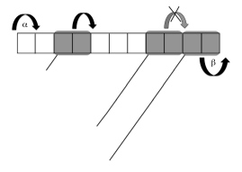
In order to take into account the steric hindrance of one machine against another, we represent each by a rigid rod of length in the unit of the lattice constant. Therefore, each machine can cover lattice sites simultaneously, but moves forward by one lattice site at a time. No lattice site can be covered by more than one machine at a time. The individual mechano-chemistry of each machine gives rise to an effective rate of “hopping” forward. But, a given machine can step forward if, and only if, the target site is not already covered by another machine. For convenience, the lattice is assumed to have length of which only the first sites constitute the template. Moreover, a new machine can initiate polymerization by occupying the first sites of the lattice, with a rate , provide all these sites are not covered by any other machine. Similarly, if the last sites are occupied by a machine, it terminates the polymerization by “hopping out” of the system with a rate . Thus, the traffic-like collective movement of many machines simultaneously on a single template is a TASEP of hard rods [555]. Indeed, to my knowledge, this was the first application of TASEP to a biological system [556, 557].
16 Rotary motors: generic models
Some of the most important rotary motors in a living cell are driven by ion-motive force (IMF). The motor is embedded, at least partly, in a membrane. The concentrations of the relevant ion (normally, either hydrogen ion H+, i.e., a proton, or sodium ion Na+) that drives this rotary motor, is higher on one side of the membrane than on the opposite side. A phenomenological theory, along the same lines as the linear response theory developed earlier for linear motors [372], has been attempted [558]. However, the choice of the generalized forces and the conjugate generalized currents is more subtle in this case because of the full vectorial character of the non-chemical variables.
Berry and Berg [559] developed the simplest kinetic model for IMF-driven rotary motors. It does not involve any explicit structural consideration. The three kinetic states are labelled by the letters E, A and B. In the kinetic scheme shown below
| (217) |
the forward transitions and indicate, respectively, entry of an ion from the high-concentration side and its exit to the low-concentration side of the membrane. All the other events, including rotation of the motor, which take place during the transit of the ion inside the motor are incorporated in the single transition . Although the dominant pathway would be , several other possibilities also arise because of the reversibility of each of the transitions. The rate constants are assumed to satisfy the detailed balance conditions appropriately and depend on both the IMF and the work done against the load torque. The three master equations satisfied by the probabilities for the states E, A, B, respectively, can be solved in the steady state and the angular velocity of the motor can be obtained from where is the step size, i.e., angle by which the motor rotates in one cycle.
In order to explain the mechanism of energy transduction some essential
structural features, which are shared by wide varieties of rotary motors,
should be incorporated in the model without sacrificing its generic
character. At least two different classes of such generic models for
the IMF-driven rotary motors can be conceived [560].
Stator-rotor “cross-bridge” models:
As emphasized by the schematic depiction in fig.32,
these models have similarities
with “motor-filament” crossbridge system that we have discussed in section
12. In these generic models the ions are the
analogs of ATP, while the stator and the rotor are the analogs of a motor
and the filament, respectively. In such a generic scenario, the binding and
release of the ions to the “flexible” stator not only alter its affinity
for the rotor (and hence stator-rotor binding), but also trigger
conformational changes (power stroke) that generate the torque needed
for the angular displacement of the rotor.
Non-contact stator-rotor interaction models: These models
involve neither stator-rotor binding nor significant conformational
changes of the stator. Instead, rotation is caused by the combined effects
of (i) the constraints imposed by the hydrophobicity of the membrane,
in which the motor is embedded, and (ii) electrostatic interactions of
the various charged components of the motor with the ions transiting
through it. In some of the models, each ion hops from the stator onto
the rotor and gets a ride for a part of its journey through the motor
before being offloaded. But, in the other models an ion remains confined
within the stator region throughout its transit. Since some concrete
examples of this mechanism will be discussed later in this review in
sections 27 and 28, we
do not discuss it further here.
Part II:
Kinetic models
of
specific motors
“The beauty of Nature lies in detail: the message, in generality. Optimal appreciation demands both”- Stephen J. Gould, in ref. [102].
17 Cargo transport by cytoskeletal motors: specific examples of porters
In the generic models of porters that we discussed in section 11, the track was assumed to provide only equidistant binding sites for the motor. However, in reality, a MT plays a much more subtle role which have started emerging from the X-ray studies of the motor-MT complexes [561]. Moreover, the generic models neither take into account the fact that MT consists of 13 protofilaments and F-actin is effectively a double helix (see appendix K); while “lane changing” on the former cannot be ruled out [562], tilting and twirling on the latter seems possible [563]. Motors, particularly kinesins, also play key roles as regulators of the dynamics and organization of the MT filaments [564]. Furthermore, most of the motors normally consist of more than one domain or subunit whose coordination is essential for the motility and other specific operations of the motor [565]. Besides, the motor molecules are not always in the transport competent “active” state; the mechanisms of autoinhibition and activation by binding to cargo and MT tracks shed light on their regulation and control [566]. Although head-to-tail interaction is one way of such regulation [566], tail-independent mechanism has also been reported [567]. Modeling the determinants of the directionality and processivity of the different families of the same superfamily [568] cannot be done satisfactorily without incorporating the specific distinct features of the different families of motors.
In this section we focus on the operational mechanism of a single motor taking into account its architectural design, the energetics of its interaction with the track and that with the fuel molecule, its mechano-chemical kinetic pathways as well as the mechanisms of their regulation and control [19, 569, 570, 571, 20, 572, 573, 574, 575, 576, 577, 578, 579, 580]. Intracellular motor-driven transport [581] is a crucially important process not only for the maintenance of the cell, but also for its morphogenesis. In fact, porters supply the raw materials needed for the formation of long tips of many specialized cells, e.g., neurons in animal cells, cilia in algae, fungal hyphae, etc. In this section, and a few following sections, we review not only the distinct features of single molecules of specific families of molecular motors but also coordination, cooperation and competition of motors of the same family and different families in intracellular transport.
Common features of architectural designs and mechano-chemical kinetics
All the porters share common functional features- these generate force and walk along a filamentous track. Interestingly, their functional commonality is related to some common features of their structural design and mechano-chemical kinetics.
All the cytoskeletal motor proteins have a head domain (or, motor domain) that contains a site for ATP binding (and hydrolysis); the ATPase site serves, effectively, as the “engine” of the motor where the chemical fuel is “burnt”. The track-binding sites of myosin and kinesin are also located on the head domain, but are distinct from the ATP-binding site. In contrast, the track-binding sites of dynein are located on the “antennae”-like extensions of the head domains. The identity of the ligand bound to the ATPase site (i.e., whether ATP of products of its hydrolysis) regulates the affinity of the motor for its track. The porters walk on their “heads” carrying cargo that are bound to their tail domains located at the distal end of the stalk.
The head domain of the kinesins is the smallest (about 350 amino acids), that of myosins is of intermediate size (about 800 amino acids) whereas the head of dyneins is very large (more than 4000 amino acids) [582]. The “identity card” for members of a superfamily is the sequence of amino acids in the motor domain. The members of a given superfamily exhibit a very high level of “sequence homology” in their motor domain. But, the amino acid sequence as well as the size, etc. of the other domains differ widely from one member to another of the same superfamily. The tail domain exhibits much more diversity than the head domain because of the necessity that the same motor should be able to recognize (and pick up) wide varieties of cargoes.
According to the widely accepted nomenclature, myosins [583, 584] are classified into families bearing numerical (roman) suffixes (I, II, …, etc.) [585]. According to the latest standardized nomenclature of kinesins [586] the name of each family begins with the word “kinesin” followed by an arabic number (, , etc.) [587]. Moreover, large subfamilies are assigned an additional letter (, , etc.) appended to the familty name. For example, kinesin-14A and kinesin-14B refer to two distinct subfamilies both of which belong to the family kinesin-14. Myosins and kinesins have a common ancestor called G protein [588, 589]. Dyneins can be broadly divided into two major classes: (i) cytoplasmic dynein, and (ii) axonemal dynein.
In an automobile, the site that processes the chemical fuel must be linked through “intermediate components” to the site that ultimately generates the motion. In the automobile, the breakdown of the chemical fuel in the engine is coupled to the stroking of a piston, which in turn is linked through the crankshaft and transmission to the turning of the wheels. Similarly, a motor molecule has to “sense” a nucleotide-dependent small conformational change resulting from ATP hydrolysis and amplify it to generate the power stroke. The actual moving element of a myosin and kinesin is a lever-like component. In case of myosin, this component is called a lever arm whereas the neck-linker of a kinesin serves essentially a similar role.
The typical duty ratios of kinesins and cytoplasmic dynein are at least whereas that of conventional myosin can be as small as . Unlike conventional myosin-II, which has a very low duty ratio (), unconventional myosin-V and myosins-VI have quite high () duty ratios. Myosin-X has moderate duty ratio.
In-vitro Motility assays
There are two geometries used for in-vitro motility assays [590]: (i) the gliding assay and (ii) the bead assay. In the gliding assay, the motors themselves are fixed to a substrate and the filaments are observed (under an optical microscope) as they glide along the motor-coated surface. In the bead assay, the filaments are fixed to a substrate. Small plastic or glass beads, whose diameters are typically of the order of , are coated with the motors. These motors move along the fixed filaments carrying the bead as their cargo. The movements of the beads are recorded optically.
17.1 Processive dimeric myosins
For the historic reason that the first myosin discovered (muscle myosin that belongs to the family myosin-II) turned out to be non-processive, those discovered later [646] were called “unconventional” [647, 648, 649, 650]. In this subsection, we highlight the main distinct features of two families of unconventional myosin motors that are both processive and serve as intracellular porters.
17.1.1 Myosin-V: a plus-end directed processive dimeric motor
Myosin-V is a dimeric “unconventional” myosin that moves processively towards the plus end of the actin track [651, 652, 653, 654, 655, 656, 657, 658]. Some of the key features of the mechano-chemical kinetics of myosin-V are as follows [659]: (i) ATP-binding triggers fast detachment of the head from the F-actin track, (ii) hydrolysis of ATP takes place quite rapidly, (iii) phosphate release is also fast, (iv) the ADP-bound head has high affinity for the F-actin track. It is desirable that a minimal model of myosin-V should account for all these facts.
Quantitative theoretical models of myosin-V has been developed by several groups from different perspectives and at different levels (see refs.[651, 660] for reviews). Kolomeisky and Fisher [661] adapted their generic model, which we sketched in section 11, for explaining several aspects of the experimental data on the kinetics of myosin-V. The kinetics of the motor was described by an unbranched pathway. Skau et al.[662] introduced a more elaborated 7-state kinetic model that allows the possibility of branching of the pathway thereby giving rise to a futile cycle in addition to the main productive cycle of myosin-V. This kinetic scheme is closely related a qualitative model, developed earlier by Rief et al. [659], except that two additional features have been incorporated: (i) futile cycle, and (ii) detachment from the track. The mechanical stepping was assumed to take place in two sub-steps: a working stroke of size nm and a diffusive excursion through nm. Both the average velocity and the run length were calculated as functions of ATP concentration and load force.
In the discrete kinetic model studied by Wu et al. [663], the
rear head can exist, at a time, in one of the following 4-distinct
states:
: the ligand-binding site is empty and the head is attached to the
F-actin track;
: the ligand-binding site is occupied by ADP and the head is attached
to the F-actin track;
: the ligand-binding site is occupied by ATP and the head is attached
to the F-actin track;
: the ligand-binding site is occupied by ATP and the head is detached
from the F-actin track.
On the other hand, the leading (front) head is assumed to be in one of
the only two states, namely,
and in which the head is occupied by ADP and is bound to
the F-actin track strongly and weakly, respectively.
Thus, in this model, the homo-dimeric motor has 8 distinct kinetic states;
a 2-letter code is used to describe these states where the letters on the
left and right represents the states of the rear and front heads,
respectively. It is also assumed that a power stroke is exerted
when the leading head is in the state and that when the trailing
head overtakes the leading head and re-attaches with the F-actin track
it must be in the state . Moreover, at the end of the power
stroke, when the erstwhile leading head becomes the trailing head, the
superscript is dropped from the label symbolizing it
because the ADP-bound state of the trailing head is unique.
Thus, both the transitions and
correspond to power strokes, albeit of different sizes (see ref.
[663] for further details of the differences).
The three kinetic pathways in this model are [663]
Wu et al.’s model [663] is an extension of an earlier model proposed by Uemura et al. [665]. It is also related to another kinetic model suggested independently by Baker et al. [666]. One of the main quantities of interest calculated by Wu et al. [663] is the steady-state average velocity
| (218) |
where we have chosen the ATP-dependent transitions for writing the expression.
Another interesting feature of this model is that termination of the walk can take place from the states and . Since the overall rate of termination is
| (219) |
the average run length is obtained from
| (220) |
Wu et al.[663] examined the trends of variation of and with the concentrations of ATP and ADP.
Figure NOT displayed for copyright reasons.
For modeling the mechano-chemical kinetics of myosin-V, Bierbaum and Lipowsky [664] adapted the Lipowsky-Liepelt model [614, 615, 481], which was developed earlier in terms of a network of mechano-chemical states, and applied successfully to dimeric kinesin. In this model each head can be in one of the three distinct states: ATP-bound (T), ADP-bound (D) and empty (E). Thus, in principle, the 2-headed myosin-V should have 9 distinct states (see fig.33). However, identifying the dominant pathways, Bierbaum and Lipowsky [664] reduced the number of distinct states to 6, namely, EE, ET, ED, DD, DT, TD. Moreover, the only 6 chemical transitions and 2 mechanical transitions (which swap the two motor heads) were allowed in this reduced description (see fig.34).
Figure NOT displayed for copyright reasons.
Denoting the six distinct states at position by the integer indices 1-6 and the corresponding states at by the primed indices 1’-6’, the mechanical transitions were represented by and (see fig.34). The average velocity of the motor was calculated from , where nm is the step size. Moreover, assuming that detachment of the motor is most likely from the state (labelled by the index 1), and with rate , the average run length was calculated from . Force-velocity relation was also computed by incorporating the force-dependence of the rate constants through the usual exponential factor.
Purely kinetic models of the type discussed above assume, rather than
explain, the processive hand-over-hand stepping pattern of myosin-V.
Lan and Sun [667, 668] developed a coarse-grained model of
myosin-V which captures the essential features of its structural
design and energetics. The state of each motor domain is described
[668] in terms of two mechanical variables
and a chemical variable (). The mechanical variables
and are the angles shown in the
fig35. Moreover, each motor domain can exist in one of the
distinct chemical states, i.e., () can take one of the
distinct allowed values.
Figure NOT displayed for copyright reasons.
In this model the dynamics of the mechanical variables can be formulated in terms of the Langevin equation, or equivalent Fokker-Planck equation, in the overdamped limit. Assuming a physically motivated form of the energy , the corresponding torques were obtained by evaluating the appropriate derivatives. For example, is the torque in the -direction. These torques were then used in the stochastic equation of motion (e.g., Fokker-Planck equation) for the mechanical variables. A master equation is ideally suited to describe the stochastic kinetics of the discrete chemical states.
Lan and Sun [668] split the elastic energy of the homo-dimeric myosin as
| (221) |
where is the separation between the two heads of the myosin and is the externally applied load force. For the elastic energy of the single myosin head labelled by (), they assumed the explicit form where is a -dependent preferred angle and the -dependent constant accounts for the differences in the free energies of different chemical states even when . The term is the elastic energy of the chain domain that links the two motor domains. Note that is independent of and because this elastic energy is independent of the chemical states of the motor domains. When both the motors are bound to the actin filament, depends on , the separation between the binding sites. A physically motivated form of the interaction energy was also assumed.
Models developed by Vilfan [669] and Xie et al.[670] are similar, in spirit, to those developed by Lan and Sun [668]. However, the details are not identical. Besides the trajectories and step size distributions, the force-velocity relation was the main quantity of interest. Following an approach similar to that followed by Lan and Sun [668] and by Vilfan [669], Craig and Linke [671] have formulated a model that provides further insight into the role of strain-induced gating in coordinating its two heads that is essential for its processivity. Few specific steps in the mechano-chemical kinetics of myosin-V have been elucidated by carrying out normal mode analysis of structural models [672, 673, 674]. Some of these structures are based on proteins data bank while others are coarse-grained elastic networks.
17.1.2 Myosin-VI: a minus-end directed processive dimeric motor
An unloaded myosin-VI walks towards the pointed end (i.e., minus end) of an actin filament whereas an unloaded myosin-V walks towards the barbed end (i.e., the plus end). For several years, the step size (36 nm) of myosin-VI was believed to be much larger than what would be expected on the basis of the prevalent interpretation of its structure at that time. In recent years this puzzle has been solved in terms of a swing of the lever arm by 1800 and special structural features of its tail domain [675, 676]. To our knowledge, only the Lan-Sun model for myosin-VI [668], which was adapted from their earlier model for myosin-V, incorporates some structural features of this motor. However, in view of the new interpretations of the structures of the lever arms and tail domains [675, 676], the theoretical model needs refinements.
17.1.3 Myosin-XI: the fastest plus-end directed myosin
Myosin-XI is, perhaps, the fastest among the myosins [677]. Just like myosin-V, it is a plus-end directed motor. But, its processivity and duty ratio are much lower than those of myosin-V motors [678]. Although the relevant thermodynamic and kinetic parameters that characterize myosin-XI have already been extracted from experimental data [677, 678], no Markov model for this kinetics have been reported so far. It would also be interesting to develop a coarse-grained model or, at least, a mechano-chemical model model of myosin-XI that would correlate its fast kinetics with the dynamics of its structural components.
17.2 Processive dimeric kinesin
The structures and mechanisms of all the kinesin families have been summarized in several reviews [591, 592, 593, 586].
17.2.1 Plus-end directed homo-dimeric porters: members of kinesin-1 family
Key structural features of kinesin-1
If the walk of a kinesin-1 is dominated by power stroke, then a mechanism for translating chemical changes (ATP hydrolysis) into mechanical movements must exist in kinesin just like that in myosin.
As we explain below, a nucleotide-dependent small conformational change of kinesin is “amplified” to generate its power stroke [20, 21, 594]. A “sensor-element” in kinesin senses the main enzymatic transitions and then relays this information to the track-binding interface and the “mechanical element” which is responsible for the mechanical movement. This pathway operates in reverse as well, because track-binding or strain on the “mechanical element” can affect rates of enzymatic reaction.
The nucleotide-binding site:
In order to change conformations between ATP- and ADP-bound states, motor proteins must sense the presence or absence of a single phosphate group. From the structural studies the “-phosphate sensor” was identified by comparing structures with and without bound ATP analogs. The sensor consists of two loops called switch I and switch II. Very similar switch loops also operate in myosin as well as in G-proteins indicating that switch loops are, from evolutionary point of view, ancient and existed even before the appearance of molecular motors.
Piston-like motion of a helix: a relay element
Small movement of the “-phosphate sensor” are transmitted to distant regions of the motor protein using a long helix that is connected to the switch-II loop at one terminus. Since the helix is long, but practically incompressible, it works like a piston. This helix is a key structural element in the communication pathway linking the catalytic site, the track-binding site and the mechanical element; the mechanical element for a kinesin is the “neck-linker” which we describe below.
Neck-linker: the mechanical element
The neck-linker (NL) of a kinesin is a region adjacent to its “catalytic core”. The NL consists of about 15 amino acids. Since it is connected to a “coiled-coil” dimerization domain its motion in one head of kinesin gets conveyed to the other head by a mechanism mechanism that we’ll discuss below.
The mechanism of the coordination of the two heads has been at the focus of intense experimental investigation over the last decade [595, 596, 597, 598, 599, 600, 601, 602, 603]. This coordination is now viewed as a “gating” phenomenon. The main idea behind “gating” is that one of the two heads has to wait till the other head opens a “gate” that allows the waiting head to resume the steps of its own mechano-chemical cycle. In principle, the gate can be operated in at least two different ways [603]: (i) polymer gate: by the attachment or detachment of the gate operator head to the MT track, or (ii) nucleotide gate: by the binding or hydrolysis of ATP or unbinding of ADP (and/or Pi) from the gate operator head. Moreover, there are two possible choices for the gated head [604, 602]: it could be the front head or the rear head. Although several plausible mechanisms of gating have been postulated [604, 602, 603, 605], the range of their validity remain controversial.
The forward bias for re-attachment of the unattached head seems to arise from the free energetics and conformational kinetics of the NL. The key feature of the neck linker is that it can “dock” on a head, i.e., it can bind to the head aligning itself towards the forward direction of motion. ATP-binding with the forward head triggers “zippering” and “docking” of the NL on it. This docking, in turn, drives the detachment of the rear head from the track and powering its forward swing towards the next binding site on the track ahead of the bound head. Thus, the NL is believed to be involved in both “gating” and forward “biasing”. The effects of length, charge and structure of the NL on the speed and processivity of kinesin-1 have been investigated experimentally by Shastry and Hancock [606]. Subsequently, they have also studied the effects of NL length on the processivities of some other families of kinesins [607] that we discuss later in this review.
Detailed kinetic model of kinesin-1
Fisher and Kolomeisky [608] adapted their generic model, which we discussed in section 11, for explaining several aspects of the experimental data on the kinetics of kinesin-1.
The generic models of 2-headed motors that we discussed earlier either directly or indirectly assumed a processive hand-over-hand stepping pattern rather than explaining how this pattern emerges from underlying molecular interactions and kinetic processes. More specifically, the Peskin-Oster model [491] assumed (i) a “gating” mechanism, whereby the front head waits in its MT-attached state while the rear head detaches from the MT and searches for a nearby binding site for its re-attachment; and (ii) a “biasing” mechanism whereby re-attachment of unattached head in front of the attached head is more probable than that of the unattached head behind the attached head. For any model developed specifically for 2-headed kinesin, it would be desirable to incorporate the molecular mechanisms of “gating” and “biasing” explicitly within its kinetic scheme.
In contrast to the models that assume tight coordination between the two heads in a hand-over-hand stepping pattern, Xie et al.[611] proposed a model in which the two heads are partially coordinated. Because of such partial coordination both backward stepping and futile ATP hydrolysis are possible in this model. Based on their recent experiments, Clancy et al.[612] have proposed a 5-state kinetic model (see fig.36) that incorporates not only both forward and backward steppings, but also futile cycles.
Figure NOT displayed for copyright reasons.
Following the steps prescribed by Chemla et al. [439], which we have discussed in section 9, Clancy et al. [612] also calculated the average velocity and randomness parameter analytically for this 5-state kinetic model. A model for the hand-over-hand stepping pattern of dimeric kinesin was developed by Shao and Gao [613] by formulating the equations of motion of the two heads in terms of Langevin equations. A network model for the same motor has been developed by Liepelt and Lipowsky [614, 615, 433] in which the kinetics is formulated in terms of master equations.
In some simplified models the NL is not incorporated explicitly, only its effect is captured in a simplified manner. For example, Mogilner et al. [609] extended the Peskin-Oster model [491] by assigning 3 possible states to each motor head, namely, the zippered state, unzippered state and the strained state. Wilson [610] models the effect of NL through a “switch”; activation of the switch mimics the zippering of the NL whereas unzippering of the NL is indicated by the deactivation of the switch. (See also ref.[619, 620]).
Derenyi and coworkers [621, 622] have developed a theoretical framework that incorporates the effects of the docking and undocking of the NL in terms of a freely-jointed-chain (FJC) model for the NL. Each head is assumed to have 6 possible states: in addition to the detached state, there are five possible attached states, namely, ATP-containing NL-undocked state (T), ATP-containing NL-docked state (T∗), ADP-containing NL-undocked state (D), ADP-containing NL-docked state (D∗), nucleotide-free NL-undocked state (0). The distinct states of the dimeric kinesin were plotted on a two-dimensional state space each axis of which depicts all the mechano-chemical states of one of the two heads. The rate constants for the transitions among the states in this state-space of the dimeric kinesin were derived from (i) the force-free rate constants for a monomeric kinesin head, and (ii) properties of the FJC model of the NL. Imposing some criteria for extraction of the parameters in an optimization procedure, Czovek et al.[622] observed that over a narrow range of the parameters, the model could account for observed data. FJC model is not the only way in which the effects of the NL can be incorporated. Alternative formulations that treat the NL either as an elastic spring or as a worm-like chain have also been developed [616].
Most of the models that incorporate NL are quantified in terms of either master equation or equivalent Brownian dynamics. However, a clearer picture may emerge if an model with structural details could be simulated. Data obtained from simulations of some structural models, performed under restricted conditions [617] indicate the important regulatory roles of the elastic strain in the NL. Recent Brownian dynamics simulations incorporating electrical charges of the amino acids indicate enhancement of the forward bias of kinesin motors by their electrostatic interactions with the MT track [618].
The free energy difference between the docked and undocked conformations of the NL is about 5 pN nm [623]. One of the controversial issues is how such a small free energy can drive a forward stepping of the motor by 8 nm against a load force as large as 5 pN [624, 625, 626]. Carrying out a Brownian dynamics simulation of a coarse-grained model with hydrodynamics interactions, Zhang and Thirumalai [627] demonstrated that, in this model, the distance of 16 nm covered by the trailing head of a kinesin-1 in a single step involves three major stages. In the first stage, the NL docks driving translocation of the trailing head by about 5-6 nm. In the second stage, the trailing head moves ahead by another 6-8 nm by anisotropic translational diffusion. Finally, in the third stage, an optimal interaction of the trailing head with the MT and its eventual binding completes its forward movement by 16 nm in a single step. The importance of (biased) Brownian motion resulting in part of the stepping of kinesin-1 has been known for many years [628]. However, interpreting the entire stepping process in terms of a pure Brownian ratchet-and-pawl device [629, 630, 631] is an interesting, but controversial, idea.
On those occasions when a cargo-carrying kinesin-1 has only one of its heads attached to the track, thermal fluctuation can lead to its detachment from the track rapidly followed by a re-attachment. However, the re-attachment need not take place at its original location because of its possible displacement during the detached state resulting from relaxation of its elastic strain. Such a process of detachment and rapid re-attachment would manifest as “hopping” of the motor [632]. The effects of hopping on the processivity and force-velocity relation has been examined theoretically using a 4-state kinetic model [632].
Limping gait of dimeric kinesin
The fact that the steps of a heterodimeric kinesin can alternate between a fast and a slow one [633] may not sound very surprising. However, what is even more surprising is that a similar stepping pattern was observed even for a homo-dimeric kinesin with genetically shortened stalk [634]. The alternating short and long dwell times is such that, for sufficiently short stalks, the longer dwell time could be about an order of magnitude longer than the shorter one. In analogy with limping gait of macroscopic bipeds, the pattern of alternating fast and slow steps of the artificially constructed kinesins were also called “limping” [602]. By performing a series of careful experiments Fehr et al.[635] ruled out several mechanisms speculated earlier for explaining limping of kinesin. The experimental observations were found to be consistent with a kinetic model proposed by Xie et al.[636]. In this model the differences in the two successive steps arise from the different vertical forces acting on the kinesin head in the two steps. Structural origin of the limping has been established by FRET measurements implicating the direct interaction of the neck linker with the MT track for the asymmetry [637].
The possible consequences of vectorial loading of a motor were analyzed by Fisher and Kim [638, 639] from theoretical considerations assuming, however, perfect symmetry between the successive steps. This analysis was subsequently extended by Zhang and Fisher [640] in the light of the insights gained from experimental investigations of limping [635]. Zhang and Fisher [640] introduced the concept of limping factor, a quantitative measure of the limping. Suppose, is the dwell time at the -th step. Then,
| (222) |
are the total dwell times at the odd and even steps, respectively. Zhang and Fisher [640] defined the limping factor by
| (223) |
The intrinsic limping factor is defined by the limiting value
| (224) |
where the angular brackets denote average over many runs (i.e., many independent sequences of 2 steps). This quantity was calculated analytically for a stochastic kinetic model of kinesin that captures the asymmetry of the stepping rates. A more detailed mechano-chemical model was developed, and treated numerically, by Shao and Gao [641].
17.2.2 Plus-end directed hetero-trimeric porters: members of kinesin-2 family
Trimeric members of the kinesin-2 family consists of two different motors and a non-motor subunit. These are plus-end directed processive motors. KIF3A and KIF3B, together with kinesin-associated protein 3 (KAP3), form a hetero-trimeric complex [642]. Another example is KLP11/KLP20 which makes a hetero-trimer by associating wih the kinesin-associated protein 1 (KAP1) [643] These motors can be collectively represented as where and are the two different types of motors. A more elaborate notation would be where and denote the head and stalk-tail domains of each motor separately. Two artificial homo-dimeric constructs and as well as a doubly-heterogeneous construct have been used in experiments [644] for a comparative study to understand the distinct roles of the different head and tails domains in the speed, processivity and force-generation of the wild-type motors [642, 643, 644]. The effects of the length of the NL on the processivity of kinesin-2 motors have been reported by shastry and Hancock [606].
Das and Kolomeisky [645] extended the generic model developed by Fisher-Kolomeisky to incorporate the distinct features of the two motors. Corresponding to a 2-state model for homo-dimeric motor and another distinct 2-state model for the homo-dimeric motor , each with step size nm, they formulated a 4-state model, with an effective step size nm, for the hetero-dimeric motor .
17.3 Single-headed myosins and kinesin
17.3.1 Single-headed kinesin-3 family
In the initial investigations, kinesin KIF1A, a member of kinesin-3 family, was an enigma. It was found to be practically as processive as a kinesin-1. But, it is a single-headed motor. Therefore, its processivity cannot be explained by any mechanism similar to the coordinated hand-over-hand stepping pattern of the 2-headed motors. Another puzzling feature of KIF1A is its step-size distribution. It can step both forward and backward although forward steps are taken more often that backward steps. Moreover, in both the directions, its step size is not restricted to only 8 nm; steps size up to 32 nm, in the integral multiples of 8 nm, have also been observed.
In the mutants of KIF1A constructed by Hirokawa, Okada and collaborators the number of charged amino acid residues in the so-called K-loop of the motor was varied systematically to investigate the effects on its processivity. Moreover, the effect of removing the charged E-hook of the tubulins was also explored. On the basis of these experiments and other complementary structural studies, it was established (see ref.[679] for a review) that The processivity of KIF1A arises from the electrostatic attraction between the oppositely charged K-loop of KIF1A and E-hook of the tubulins. Experimental data indicated that the mechano-chemical cycle of a KIF1A can be divided roughly into two different parts: in one of these the motor is strongly attached to the MT track whereas in the other it is weakly tethered to the MT while executing an, effectively, one-dimensional Brownian motion. The overall mechanism of energy transduction by KIF1A is a physical realization of the abstract Brownian ratchet mechanism that we discussed in section 6. This mechanism is captured by the 2-state stochastic kinetic model of KIF1A developed by Nishinari et al. [680, 681, 682, 683] (from now onwards, referred to as the NOSC model). All the kinetic parameters of the NOSC model were extracted from the data collected from single molecule experiments. The dwell time distribution of the single-headed KIF1A has been calculated by Garai and Chowdhury [683] using this NOSC model. Furthermore, the model can account also for the effects of steric interactions between the motors at higher concentrations when traffic congestion takes place on the MT track. The phase diagram of the NOSC model was plotted in a space spanned by experimentally accessible parameters [680, 681]. In principle, a single-headed motor like KIF1A in-vitro can change its “lane” by shifting to a neighboring protofilament on the same MT at the end of a single mechano-chemical cycle. The consequences of such “lane changing” on the KIF1A traffic has been explored theoretically [682].
Xie and collaborators [684] have extended the generic Brownian ratchet type models of molecular motors to develop a stochastic kinetic model specifically for KIF1A. The kinetics is formulated in terms of the Langevin equations that needs the shape of the potential(s) as input. In the spirit of Brownian ratchet models discussed in section 8.3.2, Xie et al.[684] assumed sawtooth and its variants at different stages of the cycle depending on the nature of the bound ligand.
17.3.2 Single-headed myosin-IX family
Myosin-IX is a plus-end-directed motor [685]. Just like KIF1A, myosin-IX family members also appear to move processively along actin filaments in spite of being single-headed motor. The mechano-chemical kinetic model proposed by Xie [686] for this single-headed motor is very similar to the model he developed earlier for single-headed kinesins [684]
17.4 Processive dimeric dynein
In this section we consider only cytoplasmic dynein [687, 688, 689, 690] because it functions as a porter in a cell (see Gibbons [691] for a history of the discovery of dynein). Dynein is a minus-end directed porter. Surprisingly, the cytoplasmic dynein alone is capable of minus-end directed cargo transportation whereas for the plus-end directed transportation several different families of kinesin participate. The dynein can transport diverse cargoes because of its regulation by many different molecular adaptors [692, 693].
Each dynein operates as a homo-dimer. The nomenclature for dynein has been standardized [694]. Its large head consists of 6 domains arranged in the form a ring that is a typical characteristics of the members of the AAA+ superfamily of ATPases [695, 696, 697, 698, 699, 700, 701, 702]. However, compared to the other members of the AAA+ superfamily, the ring-like head of a dynein has an unusual structure and enzymatic function [696]. First, four of the six modules contain sites capable of binding ATP whereas the remaining 2 modules are believed to play only regulatory roles (see fig.37).
Figure NOT displayed for copyright reasons.
Secondly, from this ring-shaped head a stalk and a tail protrude. Unlike kinesin and myosin, the head of a dynein does not bind directly to its MT track. Instead, the small globular tip of a 12- to 15-nm long stalk, that projects approximately radially outward from the ring-shaped head, binds with the MT. Since the distance between an ATPase site and the corresponding MT-binding site of a dynein is much longer than those of myosin and kinesin, the mechanism of communication between the ring-like head and the globular tip of the stalk remains controversial [703]. In fact, questions on the intra-molecular communication in dynein can be posed in three categories: [704, 703, 705]: (i) communication between the modules of the ring-like head, (ii) communication between the ring and the linker, (iii) communication between the ring and stalk.
The head is connected to the cargo-binding tail by a linker that is believed to functions as a mechanical lever in the force generation process [706, 707]. An alternative mechanism, in which the ring works like a winch, has also been suggested [708, 707]. Dynein seems to have a “gear” that controls its step size in response to load force [709]. In the absence of any load force the step size is predominantly where nm. When subjected to a sufficiently low load force, the most probable step size first decreases to and, on further increase of the load, it decreases to . Finally, it attains the smallest step size at even higher load. The stepping pattern of dynein is also quite unusual and appears very different from the standard hand-over-hand pattern followed by processive dimeric kinesins and myosins [710].
Dynactin [711] is a multisubunit protein complex that can bind to dynein. Dynein alone is not as processive as kinesin-1. However, dynactin [712, 713, 714]. is believed to enhance the processivity of dynein by acting like a tether. A cargo may be hauled by a mixture of active motors and passive tethers. In the simplest situation where one motor and one tether transport a cargo, the passive tether can either supress the rate of detachment of the active motor from the track or increase the rate of its re-attachment to the track thereby enhancing the effective processivity of the motor [741].
Singh et al. [716] carried out a Monte Carlo (MC) simulation of a model of a single head of a dynein motor. The different AAA domains are labelled by integer indices 1-6 (see fig.38). The label C marks a non-AAA domain. ATP hydrolysis occurs primarily at domain 1. The direction of the power stroke, caused by the response of ADP from domain 1 is indicated by the thick curved arrow. The domains 2, 3, and 4 are assumed to play only regulatory roles.
Figure NOT displayed for copyright reasons.
The main assumptions are as follows:
Assumption 1: Four distinct step sizes: Singh et al.[716]
proposed that if no ATPs are bound at the secondary sites, the motor
attempts to take a 32-nm step; if one ATP is bound at a secondary site,
dynein tries to take a 24-nm step; if two ATPs are bound at secondary
sites the motor attempts a 16-nm step; and if all secondary sites are
occupied the attempted step size is 8-nm. However, because of thermal
noise, the actual step size could exhibit a distribution that has peaks
at each of the four step sizes listed.
Assumption 2: ATP-binding affinities: in the absence of any load
force, the binding affinities were assumed to be ordered as follows:
. This assumption was
implemented in the MC simulation by assigning numerical values for the
on- and off-rates that satisfy the conditions
and ,
where the superscript refers to the number of bound ATP molecules.
If ATP molecules are already bound to the head, then the
probability of binding the nth ATP to a secondary site is
, and the probability of the nth ATP
unbinding from a secondary site is
where the choice for the elementary time step was
s.
Assumption 3: Load-dependence of on/off rates at secondary sites:
It was assumed that
where is the number of bound ATP molecules and is an
adjustable length. The off-rates were treated as effectively
load-independent parameters.
Assumption 4: Load-dependence of hydrolysis rate: The rate of ATP
hydrolysis by the domain 1 was assumed to decrease exponentially with
increasing load force .
Assumption 5: Regulators’ effect of ATP hydrolysis: The rate of ATP
hydrolysis was assumed to be enhanced by a multiplicative factor if at least
one of the secondary sites is occupied by ATP.
Assumption 6: The hydrolysis of ATP was assumed to be reversible
before the actual release of ADP and Pi.
From the simulation data, Singh et al.[716] obtained the
step-size distribution. They also computed the force-velocity relation
and studied the ATP-dependence of (a) the stall force, (b) average velocity.
An alternative approach was followed by Gao [717] to account for the same phenomena (including the load-dependent step size) that Singh et al.[716] tried to explain with their model. Gao introduced two coordinates: a physical coordinate and a chemical coordinate . The coordinate denotes the position of the motor along the MT track. In contrast, represents the “conformational changes” that control the chemical processes like ATP binding and hydrolysis as well as the release of ADP and Pi. Since both and were assumed to vary continuously, two separate overdamped Langevin equations were written for the time evolution of these two variables. The forces entering into these two equations were derived from a potential profile (a landscape) which depends on the chemical state (i.e., whether bound to ATP or ADP) at that instant of time. The actual forms of the rates of chemical transition depend on and . Using this model, Gao [717] studied the ATP-dependence of step sizes and stall force as well as the variation of average velocity and rate of ATP hydrolysis on the load force and ATP concentration. The experimentally observed gear-like function of dynein [709] is explained in this model to be a consequence of the loose chemo-mechanical coupling [717].
Figure NOT displayed for copyright reasons.
Tsygankov et al.[718] combined the kinetic model that they developed earlier for dynein’s ATP hydrolysis cycle [719] with a coarse-grained structural model to formulate a full mechanochemical model for a hand-over-hand stepping model of a homodimeric dynein. Based on the assumption that a dynein does not step sideways to any other protofilament, the model model describes its mechanical dynamics in a two-dimensional space (see fig.39). The AAA+ ring of each head is modeled as a circle of a fixed radius. Moreover, both the stalk and the tail are assumed to bendable, but inextensible. Furthermore, the tail is assumed to emerge tangentially from the AAA+ ring whereas the stalk is assumed to emerge perpendicularly from the same ring. Thus, the structure of each head is described by 6 variables. () are the cartesian coordinates of the center of the ring and several angular variables. The angle describes the rotation of the ring around its center. The angles and , which characterize the curvature of the stalk and tail, respectively. The angle , which is a quantitative measure of the relative position of the stalk and the tail, takes two distinct mean values in the pre-stroke and post-stroke configurations. The angle between the stalk and the MT track is denoted by whereas the relative orientations of the heads at the point of tail junction is denoted by . The variables describing the structural features evolved following Langevin equations. The 6 discrete biochemical states of each head were denoted by where T and D correspond to ATP-bound and ADP-bound states, DP describes the state bound to both ADP and Pi while indicates empty site. The asterisk indicates post-stroke state conformations. These biochemical states were updated according to the corresponding master equations. A multi-scale modeling approach was followed by Serohijos et al. [720] for studying dynein at different levels of spatio-temporal resolution. Zheng [721] carried out a normal mode analysis of a coarse-grained elastic network model of dynein establishing the key role of a closed AAA3-AAA4 interface in the mechano-chemical coupling in dynein.
17.5 Collective transport by porters
In living cells, common cargoes are vesicles, organelles, etc. However, a dielectric bead is often used as a cargo while performing experiments in-vitro. At least some motors are known to associate with other accessory proteins and/or macromolecular complexes that serve effectively as adaptors which can alter the intrinsic properties of the motors. The molecular link between the cargo and the cargo-binding domain of the motor is normally elastic. In most of the theoretical treatments [722, 723, 724] this link is modelled as a harmonic spring. In principle, the cargo would be free to move in three dimensions although the motor transporting it would walk on a linear filamentous track. However, for simplicity of modeling, the cargo may also be restricted to move only in one dimension that is parallel to the track of the motor. However, the position of the center of mass of the cargo is a continuous variable while the motor moves forward only in discrete steps.
One of the common features of these cargoes is that these are much bigger than the individual motors that haul them. Therefore, the cargo can mediate interaction between the motors giving rise to collective effects. In this subsection we review the progress in understanding some of the effects of cooperation and competition among the porters involved in intracellular transport [725, 726]. The type of the collective phenomenon depends on the nature of the cargo, viz., whether the cargo if “hard” or “soft”; we define the “hardness” and “softness” in the appropriate contexts below. In principle, the collective properties of the motors [727] are likely to depend on the following single-motor properties: (i) the processivity of individual motors, and the force-dependence of the detachment (and, attachment) rates, (ii) single-motor velocity and, more generally, the force-velocity relation, (iii) rule for load-sharing by the motors.
17.5.1 Collective transport of a “hard” cargo: load-sharing, tug-of-war and bidirectional movements
When a single “hard” cargo is hauled by more than one motor of the same type (i.e., either all kinesin or all dynein) along a single MT, it does not deform in shape. In contrast, a “soft” cargo would get elongated when pulled by the motors. A real intracellular cargo is never rigid, but the softness may vary from one cargo to another. The motility and shape change of the cargo by the collective effect of the teams of porters is a relatively new area of investigation [728, 729].
Co-directional motors: load-sharing and cooperation
How do the average velocity and the run length of such a cargo scale with the number of motors? Note that the total number of motors engaged in pulling the motor is not constant, but keeps fluctuating with time because of the detachment and reattachment of the individual motors. Suppose is the maximal number of motors that can engage simultaneously with a single hard cargo. If a load force is applied against the cargo, how does the collective force-velocity relation vary with the variation of the parameter ? This issue remains controversial in spite of many experimental investigations over the last decade. Moreover, the dependence of multi-motor cargo transport on the single-motor velocity has just begun to receive attention [730].
A kinetic model for this phenomenon was developed by Klumpp and Lipowsky [731]. In the model the load on the cargo is assumed to be shared equally by the motors (mean field approximation). A master equation is written for , the probability that the cargo is bound to the filamentous track by () motors. This theory predicted an increase in the run length of the cargo with increasing maximal number of motors . Assuming a linear force-velocity relation for each single motor, this theory also predicted a nonlinear force-velocity relation for all , where the stall force is an increasing function of . Experimental data have been analyzed within the framework of this theory [732, 733]. The effect of cargo-mediated effective assisting or resisting force on the motors was treated in a transparent intuitive manner by Wang and Li [734]. The Klumpp-Lipowsky model [731] was extended by Korn et al. [735] by allowing unequal sharing of the load by the motors. Stochastic sharing of the load by the bound motors take place in the computational model studied by Kunwar et al. [736]. In this model the motors were treated as special floppy linkages/springs. Later studies of collective transport by Kunwar and Mogilner [225] using a combination of the nonlinear force-velocity relation and the stochasticity gives rise a collective force-velocity curve that is almost linear provided at least three motors carry the load. Kunwar and Mogilner’s computational model [225] was also used by McKenney et al.[737] to investigate collective transport by dynein motors. The dependence of the collective force-velocity relation on the nature of the force-velocity relation of the individual single motors deserves further systematic thorough investigation. Kunwar and Mogilner’s [225] has been extended by Bouzat and Falo [738].
Most of the theoretical works in the early stage of investigations were based on essentially one-dimensional models. However, more recently, some of the effects of the organization of the motors on the surface of a real three-dimensional cargo has been studied by computer simulations [739].
What happens when a mixed population of co-directional fast-moving and slow-moving motors share the same track simultaneously [740]? One possibility is that the queues of motors may form behind the slow-moving ones, a well known phenomenon in vehicular traffic [495, 497]. An alternative possibility is that the faster-moving motors can increase the rate of dissociation of the slow-moving motors from the track. Indeed, as the relative fraction of the fast-moving motors is increased, a sharp transition from slow cooperative transport to fast cooperative transport is observed [740]. In a mixed population of proteins, one species may be an active motor while the other may serve as a passive tether [741]. In this case, the enhanced processivity of the cargo arises from either the suppression of the detachment or enhancement of re-attachment of the active motors [741].
Opposing motors: tug-of-war and bidirectional movements
It is well known that some motors reverse the direction of motion by switching over from one track to another which are oriented in anti-parallel fashion. In contrast to these types of reversal of direction of motion, we consider in this section those reversals where the cargo executes a bidirectional motion on the same MT track because of a “tug-of-war” between kinesins and dyneins [743, 742, 744, 745, 746]. Tug-of-war is not restricted only to kinesins and dyneins that move along MT tracks. Similar phenomena have been observed also during cargo transport by myosin V and myosin VI both of which walk along filamentous actin [747].
At least three possible mechanisms of bidirectional transport have been postulated. (i) One possibility is that either only + end directed motors or only - end directed motors are attached to the cargo at any given instant of time. Reversal of the direction of movement of the cargo is observed when the attached motors are replaced by motors of opposite polarity. (ii) The second possible mechanism is the closest to the real life “tug-of-war”; the competition between the motors of opposite polarity, which are simultaneously attached to the same cargo and tend to walk on the same filament, generates a net displacement in a direction that is decided by the stronger side. (iii) The third mechanism is based on the concept of regulation; although motors of opposite polarity are simultaneously attached to the cargo, only one type of motors are activated at a time for walking on the track. In this mechanism, the reversal of the cargo movement is caused by the regulator when it disengages one type of motor and engages motors of the opposite polarity. For experimentalists, it is a challenge not only to identify the regulator, if such a regulator exists, but also to identify the mechanism used by the regulator to act as a switch for causing the reversal of cargo movement.
Carrying measurements in live cells, Soppina et al.[748] demonstrated a tug-of-war between a single kinesin and 4 to 8 dyneins. They also speculated on how the cells might exploit the competition between a “strong and tenacious” kinesin against 4 to 8 “weak and detachment-prone” dyneins.
Muller et al.[749] extended the formalism developed by Klumpp and Lipowsky [731] for one type of motors by incorporating two oppositely moving motors. The stochastic kinetics of the system is now described by the master equation for , the probability that at time the cargo is attached with the track by plus-end directed and minus-end directed motors, respectively. Two linear force-velocity relations, with different sets of parameters, were assumed for the single motors of the two types of motors. A mathematical analysis of the steady-states of this model has been carried out by Zhang [750] in a special limit in which the numbers of motors of both species are infinite; this limit is not realistic.
The current status of the models seem to be far from satisfactory. For example, a simple stochastic model of load sharing would predict more pauses of the cargo when more motors are involved; However, this is not supported by the experimental observations [751]. It is possible that some regulatory mechanisms, which are not incorporated in the current models, have significant influence on the collective bidirectional transport of a cargo.
Force-dissociation kinetics in collective motor transport
Force-dissociation kinetics determines how fast individual motors would detach from the track under load. This kinetics plays an important role in the collective transport of a single hard cargo by many motors. In most of the theoretical works on collective motor transport the dissociation rate was assumed to be an exponentially increasing function of the applied load force. However, recent experimental results indicate that this assumption is not always valid [751].
Multi-motor hauling of single cargo across MT-MT, AF-AF and MT-AF crossings
What happens to a cargo hauled by multiple motors at a crossing of two filamentous tracks? Several possible situations can be conceived and some of these have already been investigated by experiments in-vitro [752, 753]; we list a few of these below in table 9.
| Intersection | motors |
|---|---|
| MT-MT | all kinesins |
| MT-MT | all dyneins |
| MT-MT | kinesins and dyneins |
| AF-AF | all myosin-V |
| AF-AF | all myosin-VI |
| AF-AF | myosin-V and myosin-VI |
| MT-AF | kinesins/dyneins and myosin-V/myosin-VI |
17.5.2 Many cargoes on a single track: Molecular motor traffic jam
As the cargoes are always much bigger than the motors (in-vitro as well as in-vivo), direct steric interactions of the cargoes become significant when several cargoes are carried by sufficiently dense population of motors along the same track. Such situations are reminiscent of vehicular traffic where mutual hindrance of the vehicles cause traffic jam at sufficiently high densities. In analogy with vehicular traffic, we shall refer to the collective movement of molecular motors along a filamentary track as “molecular motor traffic”; we shall explore the possibility of molecular motor traffic jam and its possible functional implications.
Most of the minimal theoretical models of interacting molecular motors utilize the similarities between molecular motor traffic on MT and vehicular traffic on highways both of which can be modeled by appropriate extensions of the totally asymmetric simple exclusion process. In such models the motor is represented by a “self-propelled” particle and its dynamics is formulated as an appropriate extension of the dynamics of the totally asymmetric simple exclusion process. In such models, in addition to forward “hopping” from one binding site to the next, the motor particle is also allowed to detach from the track. Moreover, attachment of a motor particle to an empty site is also allowed.
In reality, a molecular motor is an enzyme that hydrolyses ATP and its mechanical movement is coupled to its enzymatic cycle. In some recent works on cytoskeletal motor traffic, the essential features of the enzymatic cycle of the individual motors have been captured. Ciandrini et al.[754] developed a model where the extent of details incorporated falls in between TASEP-type model (which do not incorporate any mechano-chemistry) and those that incorporate lot of those details. Nishinari et al. [680, 681] extended the TASEP by incorporating the minimal details of the mechano-chemical cycles of individual KIF1A motors to predict their collective spatio-temporal organization, specifically jamming of motors.
17.5.3 Trip to the tip: Intracellular transport in eukaryotic cells with long tips
Motor transport in fungal hyphae
Fungal hyphae already attracted the attention of Marcello Malpighi in the seventeenth century (as evident from the graphical illustration reproduced from Malpighi’s original in ref.[755]). Most of the works on the growth of fungal hyphae focussed mainly on the biomechanics of the cell wall to predict the shape of the growing tip [756, 757]. Microtubules and cytoskeletal motors are known to play several important roles in hyphal growth in filamentous fungi [758, 759, 760]. One of the unique feature of the growth of fungal hyphae is the existence of “spitzenkörper” which is believed to play a distinct role as a vesicle supply center. Complementary investigations on the transport of materials required for this growth by the cytoskeletal motors began in more recent years [761, 762]. These models are extensions of the TASEP that incorporate the elongation of hyphae by allowing the lattice to elongate according to an appropriate dynamic rule. This extended model is called the dynamically extending exclusion process (DEEP) [762]. This model has been extended further to model bacterial flagellar growth [763]. Interesting regulatory roles of dynein has been discovered in the bidirectional transport of cargoes along fungal hyphae and quantified mathematically in terms of first passage time [764]. The queueing of the motors near the tip of a microtubule in a fungal hyphae has also been modeled by an extended version of TASEP [765].
Motor transport in plant root hair and pollen tube
Pollen tube and root hair are long extensions in plants. The transport of organelles here is dominated by acto-myosin system [766, 767]. A consequence of this organelles movements is that it gives rise to cytoplasmic streaming [768, 769]. The role of this streaming in mixing up the interior of the cell is similar to that of the molecular motors in many other situations [770].
Intraflagellar transport in algae
Flagella and cilia are important organelles in many eukaryotic cells. Eukaryotic flagella and cilia, e.g., those of green algae Chlamydomonas reinhardtii, and long extensions of some apical cells in brown algae, e.g., those of Sphacelariales are cell appendages that are shaped as a long “tip”. The history of research on these cell appendages over the last 150 years have been explored recently by Bloodgood [771]. In this subsubsection we review only intraflagellar transport (IFT) [772, 773, 774, 775, 776, 777, 778, 779, 780], a phenomenon that is driven by molecular motors, that has a much shorter history [781]. The machines and mechanisms of the undulatory motion of cilia and flagella are reviewed in section 19.3. A theoretical model of IFT has been developed by Bressloff [782]. In this model “particles” reach the tip of the cilium by hopping and elongate it by one unit.
One of the special features of cilia is that although a cilium is not an organelle in the strictest sense it is also not a continuous extension of the cytoplasm. The ciliary compartment is separated from the cytoplasmic compartment by a “diffusion barrier” [783, 784]. Very recent experiments [785] have established a close relation between the molecular components of this barrier and those on the nuclear pore complex [786] which we’ll discuss later in this review. Based on this similarity, Kee et al. [785] have proposed the existence of “ciliary pore complex”. The kinetics of crossing this barrier diffusively has not been included in any theoretical model of IFT explicitly.
Axonal transport
In a human body, the axon can be as long as a meter whereas the corresponding cell body is only about 10 microns in length. Almost all the proteins needed to maintain the synapses are synthesized in the cell body. How are these proteins transported to the synapse along the long axon [787, 788]? The problem is even more challenging in animals like elephant and giraffe which have even longer axons. A bundle of parallel MTs usually run along the axons and dendrites of a neuron, (see appendix for a brief description of the cytoskeleton of a neuron). These MTs form the track for the motorized transport of intracellular cargoes, e.g., vesicles, organelles, etc., along axons and dendrites [789, 790]. Movement of the cargo in a direction away from the cell body is called anterograde whereas that in the reverse direction is called retrograde; therefore, both kinesins and dyneins are involved [792, 793, 794] (see Fig.40).
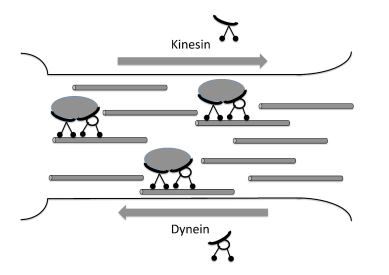
Every cargo in an axon spends a fraction of its journey time actually moving and even during those periods its movements are bidirectional. Two distinct patterns of cargo movement in axonal transport have been named “fast” and “slow” transport [795, 796]. Fast transport occurs at an average velocity of several microns per second, i.e., equivalently, several hundreds of millimeters per day. In contrast, the slow axonal transport takes place at the rate of a maximum of tens of nanometers per second, i.e., about few millimeters per day [795]. This difference may be caused by the differences in the fraction of time they spend moving although the underlying mechanism of motor transport may be the same [797]. For historical accounts of research on fast axonal transport, see ref.[798].
To our knowledge, the earliest quantitative model of axonal transport was developed by Blum and Reed [799] at a time when the nature of the key components was not clear. Subsequently, Brown [800, 797] proposed his hypothesis of “stop-and-go” traffic in axon. In order to test the basic idea of this hypothesis a quantitative model was developed by Brown et al.[801]. In this model it was assumed that (i) neurofilaments are cargo which can switch between two “relatively persistent directional states”, namely anterograde and retrograde, and (ii) in either state the neurofilaments can move or pause. Although the movements in both directions can be rapid, the overall transport is slow because the filament dwells most of the time in paused states. A slightly different dynamical model was studied by Cracium et al. [802]. In this 5-state model, the neurofilament can also be bound to a anterograde or retrograde motor that pauses while off-track. This model can be extended to a 6-state version by distinguishing between the two off-track (paused) states: neurofilament attached to an anterograde motor and neurofilament attached to a retrograde motor [803]. Possible effects of cooperativity of the motors on axonal transport have been explored [804, 805] by extending the model developed by Cracium et al.[802]. When looked at from a broader perspective, axonal transport is essentially a concrete physical realization of cooperation and competition of a group of kinesins and dyneins where the anterograde and retrograde transport observed in a specific case in an emergent phenomenon.
Effects of defect and disorder on cytoskeletal transport
We have already come across the possibility of randomness of one kind in motor traffic: the different properties of different types of motors in a mixture can be captured by randomizing the motor properties. In other words, the randomness of the motor properties have already been considered. But, so far we have implicitly regarded the track for the cytoskeletal motors to be a perfectly periodic array of motor-binding sites. However, in reality, a motor can encounter defects or disorder on its path.
17.5.4 Fluid membrane-enclosed soft cargo pulled by many motors: extraction of nanotubes
In many eukaryotic cells ER tubules are pulled out of membrane reservoirs by molecular motors that walk collectively on MT tracks [806]. Molecular motors can extract membrane tubes also from vesicles [807]. Because of the liquid-like nature of the membranes of the vesicles, the motors bound to the vesicle surface do not experience any resistance from the membrane except at the leading edge. Consequently, all the motors, except those at the leading edge, move freely along the membrane surface walking along a filamentous track. In contrast, the motors at the leading edge, because of the load force exerted by the membrane move at a slower rate. The queueing up of the faster motors behind the slower ones is analogous to queueing of vehicles in traffic [808, 809]. Thus, the assumption of equal sharing of external load, that is often used for theoretical calculations on multi-motor hauling of hard cargo, does not hold in this case. Moreover, the motors pulling the same membrane tube are not strongly coupled to each other.
The motors fail to extract a nanotube if their number density is smaller than a critical value; at densities above this critical value, motors cooperatively pull a long thin tube out of the vesicle and the tube elongates at a steady average velocity [810]. Using the formalisms of ASEP, Campas et al.[811] derived an analytical expression for the velocity of a cluster of motors denoting the forward and backward hopping rates by and , respectively:
| (225) |
where is a dimensionless parameter characterizing the position of the energy barrier between two neighboring lattice sites. Once tubulation takes place, TASEP-type models predict that the motors can exhibit varieties of dynamical phenomena [812], e.g., shocks and inverse shocks, re-entrant phase transitions, etc. The phenomenon of membrane pulling by multiple motors has been formulated mathematically also in terms of Brownian ratchets whose kinetics are governed by appropriate Langevin equations [813].
It has been argued that, even collectively, motors cannot generate strong enough force to extract membrane nanotubes if all of them move along a single protofilament; motors must be using several protofilaments simultaneously when they successfully extend a membrane tube [814]. The nature of the dynamics of the tube, however, depends on the extent of processivity of the motors [815]. For example, Ncd is a nonprocessive motor. Ncd can extract nanotubes from vesicles, but exhibits a bidirectional switching; the tube alternates between forward and backward movements with variable speeds [815]. Such richer dynamical behavior of tube extraction by nonprocessive motors is in sharp contrast with the monotonic tube growth observed when pulled by processive motors. In fact, this bidirectional motion for collective pulling by nonprocessive motors resembles the bidirectional motion of a filamentous backbone rigidly connected to multiple nonprocessive motors (which we’ll discuss in section 17.6).
17.6 Collective transport of filaments by motors: non-processivity and bistability
Consider a group of identical motors bound to an elastic backbone [816, 817, 818, 819, 820, 821, 822, 823]. Two classes of such coupled motors (motors coupled to a single backbone) have been considered. In the first, the individual motors are modeled as Brownian ratchets whereas in the second the individual motors exert a power stroke. In the first case, it has been demonstrated that even if each individual motor is non-processive, such a system of elastically coupled motors can exhibit bidirectional processive motion. In this mode of movement, the motors move collectively on a filamentary track in a processive manner in one direction for a period of time and, then, spontaneously reverse its direction of motion. Such spontaneous oscillations can account for the dynamics of axonemes, which are core constituents of eukaryotic cilia, as well as oscillatory motions of flight muscles of many insects. In the second case, several different forms of strain-dependent rates of detachment of the motors from the track have been considered.
The works cited above establish that bidirectional motion does not necessarily require pulling a cargo or a filament by antagonistic motors. A group of identical motors, each of which lacks directionality of its average motion, can give rise to a bidirectional movement of the polar filament [818]. More recent investigations have revealed that a group of identically directed motors can give rise to bidirectional movement of a bundle that consist of filaments with alternating polarities (and, therefore, apolar, on the average) [824, 825, 826, 827].
17.7 Section summary
In this section we have reviewed the kinetics of the members of several different specific families of porters as well as processes driven by single and multiple porters. Over the last couple of decades many research groups have investigated the effects of the following: (i) structural designs of the motors and the corresponding tracks, (ii) the conformational dynamics of the motor in each cycle and the (de-)polymerization kinetics of the track, (iii) the nature of the cargo and motor-cargo coupling, (iv) manner in which the load is shared by multiple motors, and regulation of oppositely-directed motors, engaged with the same cargo, and (vi) motor-traffic on the same track.
In section 2 we listed several different levels at which collective dynamics of molecular motors can be viewed. In the specific context of porters, models have been developed to study the coordination between (a) subunits of a single motor, (b) members of the same family of porters, (c) members of different families of the myosin superfamily that move in opposite directions on the same F-actin track, (c) members of kinesin and dynein superfamilies that move in opposite directions on the same MT track. We have also presented a brief review of intracellular transport in eukaryotic cells, particularly some of those with long tips.
However, the understanding of the intracellular transport in-vivo cannot be complete without integrating the MT-based transport system with the F-actin-based transport system. Although some in-vitro experiments have provided initial insights, to my knowledge, no quantitative kinetic model of this integrated transport system has been reported so far.
18 Filament depolymerization by cytoskeletal motors: specific examples of chippers
Depolymerases [140], which chip way from the tips of MT tracks, form two families of kinesins [828, 829], namely kinesin-8 and kinesin-13. Kip3p and MCAK are the two extensively studied members of these two families [830, 831]. The depolymerase activity of MCAK has received most of the attention so far [830]. Very little attention has been paid to its role as force generator [832].
Klein et al.[833] theoretically investigated the depolymerization of MT by MCAK using a one-dimensional model. The origin of the coordinate system () is permanently located at the depolymerizing tip of the MT, i.e., the description is based on a frame of reference that moves with respect to lab-fixed system. Denoting the concentration of MCAK in the bulk solution by , their MT-binding rate was assumed to be where is the maximal density of MCAK for which binding sites on the MT saturate. is the rate of detachment of the MCAK motors from the MT. The density profile of the MCAK along the MT satisfies the equation of continuity
| (226) |
where the two terms on the right hand side are the source- and sink- terms, respectively. The current density is given by the sum of diffusion and drift current, i.e.,
| (227) |
where is is the diffusion coefficient of the MCAK motors along the MT and is the sum of the average velocity of the motor with respect to the filament and is the velocity of MT depolymerization. For MCAK can be neglected. Moreover, if dimeric subunits have length and are removed from the MT at a rate , then, where is the total number of protofilaments of a MT. is expected to depend on the density of the MCAK at the depolymerizing tip of the MT; a phenomenological form of is assumed. So far as the boundary conditions are concerned, as where
| (228) |
is the equilibrium density (Langmuir formula) for motors with attachment- detachment kinetics. Similarly, another physically motivated boundary condition is specified for the boundary at . Klein et al.[833] showed that, depending on the values of the set of model parameters, MCAK motors can either accumulate at the depolymerizing end of the MT or their population there gets depleted. The dynamical accumulation of the MCAK, caused by the capturing of the motors bound along the MT filament by the retracting MT end, is a collective phenomenon. Occurrence of this phenomenon requires sufficiently high processivity of the MCAK, i.e., high probability that the depolymerizer MCAK remains attached to the MT carrying our several rounds of subunit removal before, ultimately detaching from the MT.
In the corresponding discrete stochastic model, motors are represented by particles and the MT is represented by a one-dimensional chain of equispaced discrete binding sites. No more than one particle can occupy a site simultaneously; the occupation variable can take only one of the two allowed values (empty) and (occupied). From the later equation for the occupational probabilities, one gets the rate equation for the average occupation numbers :
| (229) | |||||
where the last term essentially relabels the binding sites if the subunit at the at the MT tip is lost by depolymerization. A mean-field treatment of this model confirms the dynamic accumulation of MCAK at the depolymerizing tip of the MT provided when and the processivility is sufficiently high.
Since Klein et al.[833] considered a semi-infinite MT, their model could not be used for studying the effects of MCAK on the distribution of he lengths of the MTs. These effects of depolymerases were calculated by Govindan et al.[834]. One of the key points is that the typical “residence time” of a single depolymerase after its adsorption on the MT is on a sufficiently long MT before desorbing. Therefore, only those MCAK motors which bind to the MT within a “trapping zone” of length from the depolymerizing tip of the MT get adsorbed at the tip. Those MCAK motors which bind to the MT at a distance larger than from the MT tip get detached before getting trapped by the MT tip. Once trapped, a MCAK can escape from the MT tip only during its depolymerization activity by accompanying a subunit chipped from the MT tip.
One of the limitations of the model developed by Govindan et al. [834] is that it does not take into account the steric exclusion of the motors on the MT track, even at high concentrations of the motors. This model was extended by Hough et al.[835] incorporating the effects of steric exclusion by a prescription that was used earlier by Parmeggiani et al.[506] for modeling molecular motor traffic. Very recently jamming of MCAK motors on the MT track has been observed experimentally [836].
18.1 Section summary
In my opinion, the consequences of MT depolymerization by the depolymerase motors have been the main focus of attention of theoretical models so far. The causes of the filament depolymerization induced by these depolymerase motors has received very little attention. The difference in the modes of translocation of the members of kinesin-8 and kinesin-13 families also needs a clear explanation in terms of the differences in their structure and conformational dynamics.
19 Filament crossbridging by cytoskeletal motors: specific examples of sliders and rowers
In this section we discuss a few specific examples of sliders and rowers that are responsible for the contractility and shape changes of many cells and subcellular structures. As generators of contractile forces, acto-myosin is ubiquitous in living systems. Various modes of actomyosin contraction and the corresponding spatial and temporal patterns of force generation have been reviewed [837, 838] in the context of cell division, cell motility and morphognesis.
19.1 Acto-myosin crossbridge and muscle contraction
There are some chemical differences between the muscles of vertebrates and invertebrates (e.g, flight muscles of insects). Muscle cells of vertebrates can be broadly classified into “striated” and smooth (“non-striated”) types. Vertebrate striated muscle cells can be further divided into two categories- skeletal and cardiac. Although skeletal muscles of vertebrates (e.g., those of frog and rabbit) were used in most of the early investigations on the mechanism of muscle contraction, the cardiac muscle has been getting attention in recent years because of its implications in cardiac disease control.
Each muscle fiber is actually an enormous multinucleated cell produced by the fusion of many mononucleated precursor cells during development whose nuclei are retained in the adult muscle cell. The diameter of muscle cells is typically m and the length can range from less than a millimeter to a centimeter. Each of these cells is enclosed by a plasma membrane. The nuclei are squeezed to the peripheral region just beneath the plasma membrane.
About percent of the cytoplasm of a skeletal muscle fiber (i.e., muscle cell) is occupied by cylindrical rods of protein and are known as myofibrils. Many myofibrils, each about m in diameter, are contained within the cross section of a single muscle cell. The muscle cells also contain mitochondria sandwiched between the myofibrils.
Myofibrils are the structures that are responsible for muscle contraction. The most distinctive feature of myofibrils is their banded appearance; the dark bands correspond to higher density of protein. The spatial periodicity of the alternating light and dark bands is 2.3-2.6 m in the resting state of a muscle; the entire repeating structure, from one -disc to the next, is known as sarcomere.
The banded appearance of the sarcomere is produced by hundreds of
protein filaments bundled together in a highly ordered fashion.
The two main types of filament are:
(i) thick filaments, about 15 in diameter, are made mostly
of myosin;
(ii) thin filaments, about 7 in diameter, consist mostly of
actin.
Both these types of filaments contain also other types of proteins
which help to hold them in correct steric arrangement and regulate
the process of contraction.
Arrays of thin and thick filaments overlap in the sarcomere in a manner similar to that of two stiff bristle brushes. Myosin molecules are arranged in such a way on the thick filament that their heads point away from the mid-zone towards either end of the filament. The thick filaments come within about 13 nm of the adjacent thin filament which is close enough for the formation of cross-bridges between the myosin heads belonging to the thick filament and actin molecules constituting the thin filaments.
Research on molecular machines was focussed almost exclusively on the mechanism of muscle contraction during the first half of the 20th century and it was dominated by Archibald Hill and Otto Meyerhof [846, 847] who shared the Nobel prize in Physiology (or medicine) in 1922. We’ll not pursue the historical developments in muscle research; interestedreaders are referred to refs. [847, 848, 849, 850, 851, 852, 853, 854, 855, 856, 857, 858, 859, 860, 861, 862].
In two landmark papers published in 1954, A.F. Huxley and Niedergerke [863] and, independently, H. E. Huxley and Hanson [864] proposed the sliding filament hypothesis of muscle contraction [839]. According to this hypothesis, it is the sliding of the thick and thin filaments past each other, rather than folding of individual proteins, that leads to the contraction of the muscle. This theory was formulated clearly and quantitatively in another classic paper of A.F. Huxley in 1957. The essential assumptions of this model are as follows [865] (see fig.41):
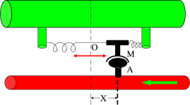
(i) Each myosin has a binding site for the actin filament of the same
cross-bridge. While unbound, the myosin executes a one-dimensional
Brownian motion parallel to the actin filament and can bind to the
filament with a rate constant where is the extension of
its elastic element.
(ii) A myosin head bound to the actin filament can detach from the
actin filament with a rate .
(iii) is moderate within a certain range of provided
; however, for . In contrast, for all
, whereas is a large constant for all
.
Let be the probability that a motor at position (i.e., with strain ) is attached to the corresponding binding site on the actin filament. Then,
| (230) |
If a steady state exists then and we have a simpler equation
| (231) |
The average force generated can be computed from
| (232) |
where is the total number of myosin motors. In principle, the force-velocity relation can be obtained by first evaluating the steady-state probability .
Does this scheme correspond to a power stroke or a Brownian ratchet? Although non-power stroke mechanism for muscle contraction has appeared in the literature in many apparently different versions (see, for example, refs.[867]), only a few interpreted the energy transduction mechanism in Andrew Huxley’s theory as a Brownian ratchet [518, 521]. The functional forms of the strain-dependent rates of attachment and detachment of the myosin motors to the actin filaments that Huxley assumed [866] is responsible for the Brownian ratchet-like mechanism. In several later papers other authors assumed more complicated functional forms of these rates (see, for example, ref.[868]) to overcome some of the limitations of the original formulation.
In the original version of the sliding filament model, developed in the nineteen fifties, it was generally assumed that the cross bridges moved back and forth along the backbone of the thick filaments remaining firmly attached to it laterally. However, later X-ray studies demonstrated that the filament separation could vary without apparently interfering with the actin-myosin interactions. On the basis of this observation, in 1969, H.E. Huxley proposed the myosin “lever arm” hypothesis [869]. This model was developed further and formulated quantitatively by A.F. Huxley and Simmons [870] in 1971 (to appreciate the status of the theory at that time see Huxley’s review of 1974 [871]).
Many subsequent extensions of the Huxley-Simmons model either incorporate larger number of chemical states of larger number of pathways. For example, a 4-state mechano-chemical kinetic model for muscle contraction, developed by Eisenberg and Hill [872], was essentially an extension of the Huxley-Simmons model [870]. In the extended version [872] that Eisenberg et al. also compared with experimental data [873], the energetics of the elastic strain and the changes in the chemical states are coupled (see ref.[874] for furher details of this approach). The importance of more than one pathways in the mechano-chemical cycle of muscle myosins was emphasized by Piazzesi et al.[875]. In recent years many powerful experimental techniques have provided deeper insight into the acto-myosin dynamics[876, 877, 878].
One of the relatively recent theoretical works on muscle contraction incorporates the cooperativity of the rowers through strain-dependent chemical kinetic processes [879, 880, 25]. The collective force-velocity relation of the rowers depends on the fraction of the bound heads . If is small, the load-free sliding velocity s large because of the successive members of a “relay teams” cooperate with each other. However, the force generated is small because only a few motors form cross-bridges at a time. In contrast, in the opposite limit of large , larger number of cross-bridges gives rise to stronger force; however, hindrance caused by the crowding of cross-bridges leads to low velocity of sliding. Many numerical as well as a few analytical treatments of the theories of various aspects of muscle contraction have been reported over the last decade [881, 882, 883, 884]
19.2 Sliding of acto-myosin bunldle in non-muscle cells: stress fibers
In non-muscle cells actomyosin bundles form stress fibers where filament sliding driven by myosin motors has strong similarity with actomyosin system in muscle cells [885, 886]. These actin bundles are involved in cell adhesion, contractility as well as in motility [887]. The stress fibers are essential components also in machineries involved in mechano-transduction. The structure and mechanism of operation of stress fibers in motile cells are different from those in non-motile (but contractile) cells [888].
The roles of chemical signaling in the alignment of stress fibers during cell adhesion has been modeled mathematically by Scholey et al. [889]. However, this model does not deal with the actomyosin crossbridges explicitly. A continuum model for the kinetics of cell contractility was developed by Deshpande et al. [890] and implemented computationally using the finite element method. This model includes (i) a simple form of time-dependence of an activation signal that triggers formation of stress fibers, (ii) an equation for the kinetics of the stress fibers where the signal-dependent recruitment of actin and myosin competes against their tension-dependent dissociation; and (iii) phenomenological equations that relate the bundle contraction (or extension) rate to the tension thereby accounting for the acto-myosin crossbridge dynamics. This model and its numerical implementation are based on fairly standard strategies of modeling and simulation in engineering for elastic continua.
Most of the models mentioned above did not incorporate the details of the signaling pathways. An attempt to capture at least some of these details was made by Besser and Schwarz [892]. They modelled stress fiber contraction by combining somewhat detailed biochemical signaling processes with the mechanics of the contractile fibers. Each sarcomeric unit of the stress fiber has been modelled by extending the Kelvin-Voigt model for a viscoelastic material. A Kelvin-Voigt unit consists of a spring and a dashpot joined in parallel. The effects of the the myosins, which slide the actin fibers, is captured by adding, also in parallel, a “contractile module” that generates a contraction force . For simplicity, a linear force-velocity relation was assumed for the motor-generated contractile force. The one-dimensional model of the stress fiber is a chain of coupled series of sarcomeric units. In the continuum limit of this chain the equation for the displacement variable satisfies a partial differential equation in which mixed derivatives of also appear [892]:
| (233) |
where the spring constant need not necessarily depend on , but the spatially-varying effective viscosity is enhanced by the motor activity. The effective stall force is assumed to depend linearly on the active fraction of the myosin heads so that attains its maximum value only if all the myosins within the cross-section at are active. The myosins get activated by a biochemical signaling pathway. The fraction is determined by solving the corresponding system of reaction-diffusion equations that describes the biochemical siganling events. One of the main predictions of this theoretical model is a heterogeneous contraction of the stress fibers; this result is consistent with experiments [892].
The models mentioned above address mostly the questions on collective behavior of the stress fibers. A model has been developed by Stachowiak and O’Shaughnessy [891] to describe the kinetics of individual stress fibers that explicitly accounts for the actomyosin crossbridges (see fig.42).
Figure NOT displayed for copyright reasons.
In this one dimensional model regions containing myosin motors alternate with regions containing -actinin. Each end of the stress fiber is connected to a transmembrane protein complex, called focal adhesion, that is anchored to the extracellular matrix. Actin and myosin (and titin) form a sarcomeric structure that resembles the sarcomere of muscles cells. Suppose denotes the length of the sarcomere. Let be the extent of overlap of the actin filaments at their pointed ends (see fig.42). The rates of polymerization of the actin filaments at the barbed ends and that of their depolymerization at the pointed end are denoted by and , respectively. It is assumed that is constant whereas increasing overlap of the pointed ends of the actin filaments increases the depolymerization rate .
Assuming, as usual, the validity of overdamped approximation, the force balance equation leads to the following equation for the sarcomere length variation with time:
| (234) |
where is the phenomenological drag coefficient. Moreover, the equation
| (235) |
imposes the length constraint, where is a characteristic force. Study of the kinetics of relaxation gets simplified by a separation of two different relevant times scales; usually, actin overlap and polymerization relax in seconds whereas the sarcomere length relaxation requires minutes [891]. The dimensionless parameter is good measure of the actin turnover rate. The experimental data analyzed by Stachowiak and O’Shaughnessy for real stress fibers correspond to . In this limit, they [891] predict that the relaxation time for the sarcomere length is .
Contact of salmonella bacteria with a host cell can activate the formation of a contractile acto-myosin machinery that resembles stress fibers. [893]. Contraction of this machinery generates sufficiently strong force that pulls the bacterium inward thereby driving the invagination of the host cell. The sarcomeric organization is not essential for the contractility of actomyosin crossbrige. Contractile actomyosin bundles, without sarcomeric organization, can arise from buckling of actin filaments [894, 895].
19.3 Sliding MTs by axonemal dynein and beating of flagella
The molecular composition, structure and dynamics of eukaryotic flagella are totally different from those of bacterial flagella. Moreover, structurally, eukaryotic flagella and cilia are qualitatively similar cell appendages; their quantitative differences lie in their size and distribution on the cell. Therefore, in the past suggestions have been made(see, for example, ref.[896]) that eukaryotic flagella and cilia should be called “undulopodia” because of their common undulatory movements.
In section 17.5.3 we have already reviewed intraflagellar transport (IFT). In this subsubsection we consider only the physical processes driven by the cytoskeletal filaments and the motors which lead to the beating of the flagella. How the various patterns of these beatings in a fluid medium propels the eukaryotic cell is a problem of fluid dynamics and will not be discussed in this article. Fir historical developments in the research on the machinery causing the beating of cilia and flagella, see for example, refs. [897, 898, 899, 900, 901].
A cilium (or eukaryotic flagellum) has a very special organization of MTs and axonemal dyneins. [908, 909, 910] The core of the machinery that drive ciliary beating is the axoneme. It consists of parallel doublet of MTs. Normally 9 such “outer doublets” are arranged so as to form the outer surface of a cylinder. Inside this cylinder, usually a pair of “singlet” microtubules runs along the axis and there are spokes that radially extend towards each outer doublet. Let us label the doublets by integer (j=1,…,N) where increases in the clockwise direction when viewed from the basal end of the axoneme. Rows of axonemal dynein form “crossbridges” between successive doublet, i.e., doublet with the doublet (j=1,…,N). Driven by ATP hydrolysis, each row of dynein slide the two doublets and with respect to each other. This sliding gets converted to a bending of the cilium because of their anchoring at the basal body and other linkages. In spite of these general features, wide variations have also been observed in the structures of cilia and flagella [911].
Many investigators have made important contributions in the theoretical modeling of flagellar and ciliary beating [909] There are some superficial similarities between muscle contraction and flagellar beating- both are driven by sliding of filaments by molecular motors [912]. A sliding filament model for flagellar beating was suggested by Brokaw [913].
Beating requires a “switching” phenomenon. Two different types of switching can be envisaged: (i) switching at temporal “switch points”, and (ii) switching at spatial “switch points” [914]. In order to complete the model, the mechanism of the switching has to be incorporated. Brokaw [913, 912] proposed a curvature control model based on the hypothesis that when the flagellum bends up to a critical curvature, it triggers the inactivation (switching OFF) of one set of dyneins and activation (switching ON) of the opposing set of dyneins.
Lindemann [915, 916, 917, 918, 919] suggested a geometric clutch hypothesis that, at first sight, may appear an alternative mechanism of switching. In this scenario, in the intact straight axoneme the dyneins are far enough from their respective binding sites so that practically no crossbridge is found. In contrast, when a flagellum bends the stretching of the nexin links, that hold the outer doubles in a ring-like geometry, generates a force transverse to the bend (t-force). This t-force squeezes some MT doublets close enough that dyneins can now form crossbridges between them. However, the dyneins now generate a torque that pushes the doublets apart thereby disengaging the active dyneins (inactivation of the crossbridges that they formed) and engaging their opposing set of dyneins (activation of another set of crossbridges). Because of their obvious analogy with clutches, this switching mechanism is called geometric clutch hypothesis.
Alternative hypotheses for switching are based on either control exerted through the central-pair spoke [920, 921], or coordinated with the dynein crossbridge cycle [922]. The role of the central pair of MTs is not fully understood, particularly because some cilia do not possess these central MTs [923].
The special 9+2 or 9+0 design of the axoneme and dynein-driven sliding of the axonemal MTs cause the beating of cilia and flagella. However, for similar beating of a bundle of MTs much fewer molecular components and simpler design seems to be adequate [924]. In their in-vitro studies, Sanchez et al. [924], used only the following main components: (i) a cluster of biotin-labelled kinesin motors by binding with multimeric streptavidin, (ii) taxol-stabilized MTs, and (iii) polythylene glycol (PEG). The bundling of MTs is induced by PEG and relative sliding of the MTs in a bundle are driven by the artificially constructed multimeric kinesin. The active MT bundles are attached to a fixed boundary that serves as the counterpart of the basal body to which the axonemes are attached in real eukaryotic cilia and flagella. In spite of several crucial differences in the components and design, the beat patterns of the active MT bundles are very similar to those of cilia and flagella [924]. The generic beating of the active filamentous bundles has been predicted theoretically [925, 926] (see also ref.[927, 928]).
19.4 Sliding MTs by dynein and platelet production
Megakaryocytes are precursor cells that reside primarily in the bone marrow. Remodeling of each megakaryocyte through a complex series of processes leads to the formation of thousands of platelets that are released into the bloodstream [929, 930, 931, 932]. The sequence of these processes begins with the formation of a long protrusion of the megakaryocyte that serves as the site of organization of a proplatelet, the precursor of a platelet. These protrusions elongate, become thinner, and branch out to form tubular projections. Alignment of many microtubules within the proplatelet leads to the formation of a bundle just under the cell cortex. These bundles loop around forming buds at the tips of the proplatelets.
Although the MT bundle keeps growing in length by ongoing MT polymerization, the proplatelet enlargement is not driven by piston-like action of the polymerizing MTs. In fact, the plus ends of the MTs are dispersed throughout the cortex of the proplatelet and not all the MTs are oriented parallelly in the bundle [930, 931, 932]. It is the sliding of the MTs relative to each other by dynein motors that is believed to be responsible for the growth of the proplatelets. Thus, platelet formation can be divided roughly into three phases: (i) emergence of the protrusion of a megakaryocyte thereby initiating the formation of a proplatelet, (ii) elongation, thinning and branching of the proplatelet, and (iii) release of the platelets from the tips of the proplatelets. The general principles of cell protrusions driven by cytoskeletal filaments and associated motors will be discussed in the next section.
In this section we briefly mention the key ingredients of a computational model that has been developed very recently [933] for primarily the stage (ii) of the process, namely the emergence of the shape of the proplatelet. This model is based on the assumption that the shape of the proplatelet is determined by a balance of the forces acting on the MT bundle that runs along its periphery. The MT bundle is modeled as node-spring loop where each node interacts with two adjacent neighbors on its two sides. Both stretching and bending result in restoring forces. The extension of the MT bundle is implemented by gradual elongation of the rest lengths of all the springs in the loop; the plausible microscopic physical origins of these elongations (e.g., MT sliding and polymerization) are, however, not incorporated explicitly. Bundling proteins, that “zipper” the MT bundles on the opposite sides of a narrow corridor of the barbell-shaped proplatelet, are mimicked by transient elastic bonds. The compressive force exerted by the cell cortex is captured by an effective pressure . Using this model, Thon et al. [933] demonstrated the effects of the initial perimeter of the proplatelet and the number of MTs in the bundle on the transition from spherical to barbell shaped proplatelet.
19.5 Sliding MTs by kinesin-5
Kinesin-5 is homotetrameric in the sense that it has four identical motor domains with a pair of motor domains at each end of a rod-like stalk. Most of the in-vitro experiments on kinesin-5 have been performed with Eg5, a member of this family. It is a plus-end directed motor. Each kinesin-5 motor can crosslink a pair of MTs such that the two pairs of its heads, located at the two ends of the stalk, walk on the two different MTs that are crosslinked by it [934].
From in-vitro experiments with polarity-labelled MTs, Kapitein et al. [935] established that parallel MTs crosslinked by Eg5 remain practically static whereas an Eg5 crosslinker slides two mutually antiparallel MTs. In the latter case the sliding velocity of the crosslinked antiparallel MTs arises from the fact that one pair of its heads walk on one of the crosslinked MTs with a velocity while the other pair of heads walk with a velocity on the oppositely oriented MT. Eg5 gets activated and its directional motility gets triggered only when it crosslinks two MTs [936]. This is very similar to the activation of kinesin-1 by cargo binding [566]; one of the two MTS cross-linked by the kinesin-5 can be viewed as the cargo for kinesin-5 while the other is regarded as a track [936].
The structural transitions and chemical steps in the ATPase cycle of individual Eg5 motors have been monitored simultaneously [937]. Monitoring the domain movements of Eg5, using FRET as the probe, Rosenfeld et al. [938] proposed a kinetic scheme for the ATPase cycle of individual heads (motor domains) of Eg5.
So far as the mechanism of force generation and stepping pattern is concerned, a comparison of the members of kinesin-5 and kinesin-1 families has been reported [939]. For example, at a given ATP concentration, Eg5 is much slower than kinesin-1 although the ATP-dependence of both follow the same Michaelis-Menten equation [939]. In order to understand the mechanisms of Eg5 and compare it with conventional dimeric kinesin-1, dimeric Eg5 (essentially, a truncated ‘half Eg5”) have been constructed genetically. At first sight, the mechano-chemical kinetics of such a dimeric Eg5 might be expected to be similar to that of a kinesin-1. But, biochemical experiments as well as single-molecule manipulations have revealed that the dimeric Eg5 is (i) slower, (ii) less processive, and (iii) less sensitive to load force than dimeric kinesin-1 [940, 941, 942, 943, 944] These differences may be consequences of the differences in the stiffness and docking/undocking of their neck linkers [938]. These structural differences may be the results of their evolutionary adaptation for distinct functional roles- full length tetrameric Eg5 motors usually work as MT sliders in small groups whereas dimeric kinesin-1 work as lonely porters [942]. A 5-state kinetic model has been proposed for the stepping of dimeric Eg5 during a processive run [944].
In order to understand the relevance of the coordination of the two heads of dimeric Eg5 constructs, Kaseda et al. [945] engineered an even further truncated Eg5 construct that has only a single head. Based on their experimental observations on this single-headed Eg5, they claimed that MT sliding driven by full tetrameric Eg5 is very similar to sliding of actin filaments by myosin-II in muscles. For any Eg5, they claim, only one of the two heads interacting with a MT generates force while the other is redundant; coordinated hand-over-hand processive walking of the two heads of Eg5 are rare events [945]. These claims are not consistent with the results obtained from single molecule experiments on dimeric Eg5. Plausible reasons for these discrepancies have been listed by Kaseda et al.[934].
19.6 Section summary
In this section we have reviewed several different motor-filament crossbridge system that display striking similarities of motor-induced sliding of cytoskeletal filaments.
Interestingly, specific power output of muscles and eukaryotic flagella are comparable. For both, large number of motors collectively slide cytoskeletal filaments although the force producers are quite different. In contrast, the specific power output of the cytokinetic furrow is few orders of magnitude lower than that of muscle in spite of the fact that both are acto-myosin systems. This difference may be a consequence of the widely different density of the myosin motors in the two systems.
20 Push / pull by polymerizing / depolymerizing cytoskeletal filaments: specific examples of nano-pistons and nano-hooks
Earlier in section 13, we have discussed only a few generic models that account for the pushing and pulling forces generated by nano-pistons and nano-hooks, respectively. In this section we discuss more explicit models for the force generation by cytoskeletal filaments in eukaryotes as well as that by their prokaryotic homologs by taking into account some of the key specific features of their structure and dynamics. The polymerizing filaments “polarize” cells, form dynamic cell “protrusions” and drive the engines of motility of single cells as well as collective migration of a group of cells.
Unicellular microorganisms have developed diverse molecular mechanisms of locomotion. The actual mechanism used by a specific type of organism depends on the nature of the environment in the natural habitat of the organisms. If a micro-organism lives in a bulk fluid, it’s natural mode of motility is swimming. In contrast, if a micro-organism lives in a thin fluid film close to a solid surface (i.e., in a wet surface), gliding should be its mechanism of movement [946, 947, 948, 949, 950]. Of course, some micro-organisms may be capable of utilizing both these modes of motility.
Unicellular eukaryotes, like free-living protozoa, move primarily for food. In multicellular prokaryotes, cell locomotion is essential in development. Moreover, leukocytes move to offer immune response. Furthermore, fibroblasts, which are normally stationary, move during wound healing. Swimming, gliding and crawling are some of the most common modes of motility of eukaryotic cells.
One of the fundamental questions on cell motility is the molecular mechanisms involved in the generation of required forces. Broadly speaking, three different mechanisms have been postulated and their possibility in specific contexts have been explored: (i) Force generated by polymerization of cytoskeletal protein filaments (actin and microtubules), (ii) Force generated by cytoskeletal motors by their interactions with filamentous tracks, and (iii) forces of osmotic of hydrostatic origin.
Since our aim here is limited to a discussion of the mechanisms of force generation by the cytoskeletal filaments and their prokaryotic analogs, and since a detailed discussion of cell motility is beyond the scope of this review, we’ll explain these phenomena only briefly and provide relevant references to the literature in the appropriate contexts.
20.1 Force generated by polymerizing microtubules in eukaryotes
Pushing force generation by polymerizing MTs has been investigated experimentally for the last one and half decades (for reviews, see ref. [951, 952, 953, 954, 955, 956, 957, 958, 959, 960]). A normal MT consists of 13 protofilaments. If the tips of all the protofilaments always touched the same obstacle, one could replace the MT by a single rigid rod. However, in reality, only a fraction of these protofilament may touch the obstacle at a time and this fraction may fluctuate because of the stochastic kinetics of the polymerization process. Thus, the load force is shared by only those protofilaments that touch the membrane. At any instant, those load-bearing protofilaments are too close to the obstacle to polymerize because the gap in between the obstacle and their tips are not wide enough to accomodate a tubulin dimer. However, by supporting a larger share of the load, these protofilaments “subsidize” the growth of those neighboring filaments whose tip is farther from the obstacle. The Brownian ratchet model [538] of force generation by filament polymerization, which we sketched in section 13, was appropriately modified by Mogilner and Oster to incorporate this “subsidy effect” [954].
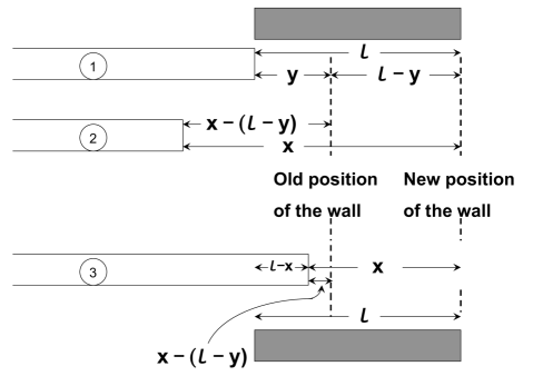
Mogilner and Oster [954] assumed that the longest protofilament can support the MT against the membrane. In this one-dimensional model the origin of the coordinate system is placed at the tip of the longest protofilament (see fig.43). Suppose, represents the number of protofilament tips at a distance from the tip of the leading protofilament at time , where , with labelling the protofilaments and nm is the length of a tubulin dimer. The protofilaments within a distance from the membrane are identified as the “working protofilaments” [954]. If the tip of a protofilament is at a distance from the tip of the leading protofilament just before a tubulin dimer assembles on its tip, then the leading tip is advance by a distance (see fig.43).
In order to get the continuum limit is scaled to the density with the constraint arising from the conservation of the total number of tips. and denote the rates of attachment and detachment of tubulin dimers at a MT tip far from the wall. In the presence of a load force , the rate of growth is altered from to . The rate equations for are [954]
(as depicted by the protofilament 2 in fig.43), and
(as depicted by the protofilament 3 in fig.43). The average velocity of the membrane protrusion can be calculated from
| (238) |
Mogilner and Oster [954] obtained not only the force-velocity relation (relation between the average velocity of MT growth as a function of the load force), but also the steady-state distribution of the tips of the protofilaments for a few distinct strengths of the load force. Predictions of both the Brownian ratchet theory of pushing force generated by polymerizing MTs, both with and without proper accounting of subsidy effect have been the subjects of many experimental studies [955, 951].
20.2 Force generated by polymerizing actin: dynamic cell protrusions and motility
Proper biological function of a cell requires appropriate spatio-temporal organization. For spatial organization within the cell, the number, size, shape and the internal environment of the organelles need to self-organize.
20.2.1 Force generation and cell protrusion by actin polymerization
Actin filaments are much more flexible than MT filaments. Moreover, these not only have a double-helical structure but also form a branched network. The Brownian ratchet model [538] was extended to the “elastic Brownian ratchet” [1029] by incorporating the interplay of bending elasticity and thermal fluctuations in the model. The space in between the obstacle and the filament can be created by the thermally induced fluctuations of the actin filaments rather than that of the obstacle. In many real situations, a subpopulation of the actin filaments remain attached to the obstacle while the remaining population are detached from it. The tethered filaments hold the obstacle while the free filaments can push it by polymerization. By capturing these two distinct populations separately in the model, the elastic ratchet model was extended by Mogilner and Oster to the “tethered ratchet model” [1031].
One distinct feature of the actin filaments is that new branches can nucleate on existing filaments thereby creating a branched network. Such branching has been modeled by Carlsson [1032, 1033]. A mesoscopic model for force generation by actin polymerization was developed by Gerbal et al.[1034]. In this model, the polymerized network of the actin filaments is described as a gel [1035] and treated as a continuous elastic medium that is anchored to the surface of the obstacle. Growth of the actin filaments is captured as addition of new layers on the gel causing compression of the previously formed layers. The release of the stored elastic energy relaxes the gel and pushes the barrier. Thus, the free energy of polymerization does not directly push the barrier; it is first stored as elastic energy which, in turn, performs the mechanical work.
Forces generated by actin polymerization [1046] not only gives rise to dynamic cell protrusions at the leading edge of a cell (see table 10) but also plays the central role in actin-based cell motility [1006, 1007, 1008, 1009, 1010, 1011, 1012, 1013, 1014, 1015, 1016, 1017, 1018, 1019, 1020, 1021, 1022, 1023, 1024]. as well as in the collective migration of a group of cells [1047, 1048, 1049, 1050, 1051, 1052]. Actin-based cell protrusions also play important roles in growth and morphogenesis of non-motile organisms like filamentous fungi [1053]. Crawling of animal cell results from a coordinated cycle of three key processes: (i) formation of cell protrusions in the forward direction, (ii) adhesion of the cell to a solid substrate, and (iii) retraction from the rear. However, in this review, we restrict our discussions only to the role of force generators in creating cell protrusions.
The actin-based protrusions of eukaryotic cells [1006, 1007, 1008, 1009, 1010, 1011, 1012, 1013, 1014, 1015, 1016, 1017, 1018, 1019, 1020, 1021, 1022]. can be broadly divided into two categories based on the nature of the actin networks: (i) branched arrays, and (ii) actin bundles [1025]. The actin networks of lamellipodia of crawling cells and the invadopodia of cancer cells are common examples of branched arrays. In contrast, the crosslinked parallel filaments in filopodia, microvili and sterocilia are examples of actin bundles. Filopodia protruding from a lamellipodium is not uncommon. Other protrusions of the eukaryotic cell include pseudopodia, ruffles, microvilli, invadopodia, etc. Although the key role in the formation of these protrusions is played by actin, the myosin motors also participate in the process, particularly in maintaining the polarity [1025].
| Protrusion | Width | Duration |
|---|---|---|
| Lamellipodium | 0.1-0.2 m | Minutes |
| Filopodium | 0.1-0.3 m | Minutes |
| Podosome | 0.5-2.0 m | Minutes |
| Invadopodia | 0.5-2.0 m | Hours |
Two different models for the formation of the actin-bundles of filopodia have been proposed. In the “convergent elongation model”, the filopodial actin filaments are assumed to originate from the lamellipodial actin network. But, in the “de novo filament nucleation model”, the filopodial actin filaments are assumed to nucleate separately in the filopodia.
A common feature of the actin networks in lamellipodia and filopodia is that the fast growing (barbed) ends of the actin filaments are oriented towards the membrane which gets pushed by the piston-like action of the polymerizing actin filaments. This piston-like pushing by polymerizing actin is very similar to piston-like action of polymerizing microtubules, which we discussed earlier, except that actin can form branched structures whereas microtubules do not. Moreover, actin-capping proteins [1026] can block the barbed ends of the actin filaments thereby increasing the concentration of monomeric actin which can be channelled towards the faster growth of non-capped actin filaments [1027]. But, processive cappers like formin protect the barbed ends from capping proteins thereby enabling the formation of long actin filaments [164]. The role of the elastic energy of the formin-capped barbed end in the diversity of the actin polymerization rates have been studied theoretically [1028]. From the perspective of transport, long-distance movement of a processive capping protein at the tip of a polymerizing actin filament can be viewed as a molecular motor powered by actin polymerization [164]. Theoretical models developed for the dynamic cell protrusions have been reviewed extensively [1029, 1030, 1031, 1045, 1032, 1036, 1037, 1038, 1039, 1040, 1041, 1042, 1043, 1044, 1018].
Force generated by depolymerizing MSP in nematodes
The uterus of a nematode female is normally packed densely with eggs. Therefore, it would be extremely difficult for a nematode sperm to swim under these conditions. Perhaps, that is the reason why, instead of swimming like in other eukaryotes, the sperm cell of nematodes crawl [961]. However, a more interesting feature of nematode sperm motility is the fact that it does not possess actin! Instead, a protein, called major sperm protein (MSP), acts like actin [962, 963] forming dynamic filaments which drive the motility of the cell [964]. However, in contrast to actin filaments, the individual filaments of MSP have no polarity. Therefore, these cannot serve as tracks for any motor proteins (or their analogs).
There are patches on the individual filaments of MSP which cross-link filaments into “bundles”. Ideas similar to “tethered ratchet”, developed originally for actin filaments, could be adapted to explain the mechanism of cell protrusion by MSP filament bundles in the leading edge of the nematode sperm [965, 966, 967, 968]. However, in the absence of myosin and analogous motor proteins, an altogether different mechanism had to be invoked for the observed retraction of the rear of the nematode sperm [969]. This mechanism of force generation by depolymerizing MSP bundles is a physical realization of the generic mechanism outlined [534] in section 13. A pH gradient was postulated to regulate MSP assembly at the leading edge and disassembly at the rear. More recently, biochemical kinetics that regulates the biophysical processes of force generation has been incorporated in a model [970]. Besides, an alternative plausible scenario of MSP assembly has been proposed [971] to explain the motility of nematode sperm cells.
Force generation by depolymerization of type-IV pili in bacteria
Myxobacteria have two different types of engines at their two poles. One of these assembles type IV pili, a class of dynamic appendages, whose retraction propels the cell forward and the corresponding mode of motility is called twitching [972, 973, 974, 975, 976, 977]. A typical type IV pilus is 6 nm thick and can extend up to about 5 m from the surface of the cell. In rod-shaped bacteria, these appendages are normally located at the cell poles. A pilus is a polymeric helical filament consisting of pilin subunits. [972, 973, 978, 979, 980, 981, 532, 982]
Suppose, polymerization of a pilus is energy-consuming whereas the depolymerization is a spontaneous process. PilT, an ATPase, could catalyze the removal of a stabilizing cap at the base of the pilus thereby triggering its depolymerization from the base. This process of retraction of the pilus exerts pulling force on the surface to which its distal tip is tethered. Alternatively, suppose the polymerization of a pilus is spontaneous. Then, PilT can peel off subunits from its base in an ATP-dependent manner causing its retraction. In both these alternative scenario, the energy consumed does not directly pull the pilus towards the membrane. Instead, energy input assures its depolymerization at the base. Therefore, these have been called Brownian ratchet mechanism and facilitated ratchet mechanism, respectively [973]. In the power stroke mechanism, PilT walks like a ATP-fuelled motor towards the distal end of the pilus and its stepping forces the pilus directly towards its base [973].
Force generation by actin comets for motility of bacterial pathogens
A classic example of actin-based cell motility is that of the intracellular bacterial pathogens, like Listeria monocyteogenes, that are propelled by “actin comets” [983, 984, 985, 986, 987, 988, 989, 990, 991, 992] (for an historical account of its discovery, see ref[993]). In this case a comet-like tail of polymerizing actin filaments push the pathogen in the host cell. Unlike, cell crawling, which is also driven by actin-polymerization, neither adhesion to a solid substrate nor retraction of the rear of the cell is required.
20.3 Cell polarization: roles of cytoskeletal filaments and motors
Most of the living cells get “polarized” [994]. Polarization of a cell is defined as a “redistribution of multiple proteins and lipids in the cell” [1000]. Two essential properties of cell polarity are [1003]: (i) asymmetric distribution of mobile molecular species between two opposite poles of the cell; and (ii) the oriented organization of intrinsically polar cytoskeletal filaments (e.g., microtubules and actin filaments) along the axis of polarity. Polarization leads to the formation of cell protrusions which are used by a wide variety of cells for their motility. The “universal” features of polarized cells (i.e., features shared by most of the polarized cells) have been listed recently [1000]. Establishment, as well as the subsequent maintenance, of cell polarity depend, at least partly, on the dynamic assembly of the cytoskeletal filaments and the motor-driven transport that they support [1002, 1003, 1004, 1005].
Establishment of polarization of a cell may be viewed as a symmetry breaking phenomenon [995]. In biology, symmetry breaking can take place at several different levels of organization; at each level, the asymmetry can be attributed to underlying asymmetries at a lower level of organization. For example, the polarity of the polar cytoskeletal filaments arise from the asymmetry in the structure of their subunits and in the kinetics of their polymerization. Similarly, the polarity of the cytoskeletal filaments plays key roles in generating polarity of the cell which, in turn, leads to the asymmetries at the levels of tissue and the organism [995].
The process of establishing polarity of a cell can get assisted by either internal processes or by its interaction with the external environment or by a combination of the two. In the absence of any external cause, symmetry of a cell can be broken by amplification of the spontaneous internal fluctuations [995, 997]. Alternatively, a mechanical stress generated by the extracellular matrix or a bio-chemical signal sent by the surrounding aqueous medium (or a combination of chemo-mechanical interactions of the cell with its environment) can polarize it [996]. Whether a cell can polarize spontaneously or only in response to an external asymmetric signal may depend crucially on the geometry of the organization of the cytoseletal filaments [998]. The cell membrane is likely to play am important role in this process. For example, phase segregation of membrane proteins can give rise to cell protrusions if these proteins assist force generation by promoting actin polymerization [1054, 1055, 1056, 1057]. Different alternative approaches to mathematical modeling of cell polarization have been reviewed and compared in recent years [999, 1000, 1001].
Once a cell becomes polarized, how long does the polarity persist? The answer to this question depends on the type of the cell. Some cells utilize this polarity for their motility either to chase their enemies or to search for a mate. For such cells, ability to respond to temporal variations in external stimuli and corresponding adaptation requires changes in the polarization pattern. Transient cell protrusions can lead to the formation of a nano-tubes [1058, 1059, 1060, 1061] connecting two cells for their communications [1062]. In contrast, for some cells, like neuron, polarity needs to be maintained stably throughout the life time of the cell. Therefore, establishment of the polarized structure of the cell is a part of its morphogenesis. Interestingly, a single cell exhibits all the hallmarks of development of an entire multicellular organism, viz., anterior-posterior asymmetry, dorsal-ventral asymmetry as well as the formation of the overall pattern [122].
20.4 Section summary
In this section we have reviewed force generation by polymerizing and depolymerizing cytoskeletal filaments. A single MT is a stiff linear nano-tube; its polymerization involves an interesting cooperativity in the load-sharing by the leading protofilaments. In contrast, actin can form either bundles or branched network of filaments; cooperativity of the polymerization-depolymerization kinetics of these filaments dominate the emerging morphology and motility of a cell.
21 Mitotic spindle: a self-organized machinery for eukaryotic chromosome segregation
The asters and vortices observed in in-vitro mixtures of tubulins and motors, [1063, 1064, 1065, 1066, 1067, 1068, 125, 1069, 1070] have been theoretically demonstrated to be the emergent patterns [1071, 1072, 1073, 1074, 1075, 1076, 1077]. Such patterns are generic [1078, 1079] and the corresponding acto-myosin system forms not only asters, but also rings, and various typesof networks [1080, 1081]. In this section we review a self-organized machine called mitotic spindle; it may be regarded as a system of two interacting asters, and it generates forces that drive chromosome segregation in eukaryotic cells.
In eukaryotic cells chromosome segregation is preceded by the replication and condensation of chromosomes which lead to the formation of sister chromatids. The complex process whereby the sister chromatids in eukaryotic cells are finally segregated is called mitosis [1082, 1083, 1084, 1085, 1086, 1087, 1088, 1089, 1090] and is carried out by the mitotic spindle [1091, 1092, 1093, 1094, 1095, 1096, 1097, 1098, 1099, 1100, 1101, 1102, 1103]. A similar machinery, called the meiotic spindle, runs the related process of meiosis. The evolution of the main ideas on the mitotic machinery over almost one and a quarter century are well documented [1104, 1105]. An excellent review [1090] of mitosis has appeared very recently.
21.1 Mitotic spindle: inventory of force generators and list of stages
21.1.1 Mitotic spindle: key components and force generators
The spindle shape in all eukaryotic cells share some common features irrespective of the pathway that leads to its assembly. When the spindle assembly is completed, it takes its characteristic fusiform shape. It looks like an ellipsoid made of fibers which are actually bundles of MT filaments. The minus ends of the MTs are focussed into the two “poles” located at the opposite ends while the plus ends of the MTs extend towards the spindle “equator”.
Just before chromosome segregation begins, the sister chromatids remain attached with each other, mostly in a typical “X”-shaped structure. The region where the two sister chromatids are closest to each other (the intersection of the two arms of “X”-shaped structure) is called centromere. At the centromere region of each sister chromatid a protein complex of a specialized composition and architectural design is located; this complex, called kinetochore [1106, 1107], plays a crucial role in mitosis. We’ll describe its structure and function in further detail later in this section.
MTs in the spindle can be classified into two main categories on the basis of the interacting partners of their plus ends- (i) kinetochore MTs (kMT), and (ii) non-kinetochore MTs. The plus end of the kMTs attach with the kinetochores; the MT-kinetochore coupling is essential for chromosome segregation. Non-kinetochore MTs can be further subdivided into two major classes- (a) astral MT (aMT), and (b) interpolar MT (ipMT). There is another set of MTs that interacts with the chromosome arms. The aMTs radiate from the poles towards the cell cortex; they are believed to play important roles in the positioning of the spindle as a whole and in marking the plane for subsequent assembly of the cleavage furrow during cytokinesis. Two sets of ipMTs, roughly equal in number, originate from the opposite poles; these antiparallel MTs overlap and interact (possibly crosslinked by MAPs or MT-based motors) at the equatorial plane thereby linking the two halves of the spindle mechanically.
The key force generators of a mitotic spindle are [1108] (i) cytoskeletal filaments, and (ii) cytoskeletal molecular motors [1109, 1110, 1111, 1112, 1113, 1114]. The major kinetic processes involved in the force generation are (a) polymerization and depolymerization of the cytoskeletal filaments, caused by dynamics instability, predominantly of the MTs, that result in pushing and pulling forces (b) depolymerization of MTs by depolymerizers (the “shredders”), generating pulling forces [1115]; (c) relative sliding of the filaments by crosslinking “rower” and “slider” molecular motors [1116, 1117, 1118], (d) transport of molecular cargoes by “porter” motors, (e) stretching of the chromosomes or bending of cytoskeletal filaments that generate spring-like elastic forces. Although MT, MT-based motors and MAPS are the main structural and functional components of mitotic spindle and mitosis [1119], actin and myosin are also suspected to play some roles [1120]. We have reviewed the kinetic models of all these processes separately in the preceding sections. It is the integration of so many processes in cell division that poses the main conceptual challenge to theoretical modelers.
Recall that a single molecular motor generates a force that is of the order of pico-Newtons and leads to mechanical movements over a maximum of tens of nanometers. In contrast, during cell division coordination of a large number of force generators takes place thereby exerting forces as large as a few nano-Newtons and causing movements over microns to tens of microns. A satisfactory theoretical model must show how such large forces and long distance movements emerge from the cooperation and/or competition between the molecular components of the machinery of cell division.
21.1.2 Mitosis: successive stages of chromosomal ballet
The mitotic phase of cell cycle is collectively designated as the M phase. The M phase is subdivided into a sequence of several phases of shorter duration. Assembly of the mitotic spindle and its coupling with the chromosomes begins in the prometaphase and the appropriate positioning of the chromosomes in the equatorial plane gets completed in the metaphase. Chromosome segregation takes places in two stages of anaphase. During the first part of anaphase, called anaphase A, the sister chromatids are pulled apart towards the poles of the spindle while the pole-pole separation remains practically unchanged. However, in the second part of anaphase, called anaphase B, pole-pole separation keeps increasing simultaneously with the poleward movement of the chromosomes. In the next phase, called telophase, the spindle is disassembled while two separate nuclei of the two daughter cells form around the segregated chromatin. We’ll review the kinetics of the mitotic machinery mainly during the period that covers approximately the prometaphase, metaphase and anaphase.
21.2 Spindle morphogenesis
Spindle morphogenesis [1102] involves at least three positioning tasks: (i) positioning of the spindle as a whole in the parent cell, (ii) positioning of the chromosomes within the spindle in the equatorial plane, and (iii) positioning of the poles within the spindle at a certain distance from the chromosomes. Such positioning requires a subtle interplay of several force generators that are parts of the complex machinery. Positioning of poles is, however, different from the other two in one respect; it establishes a spatial scale, namely, the pole-to-pole separation which need not be determined by the cell size alone [119, 121, 122]. Studying the pole-to-pole separation in terms of the forces generated by the various force-generating components of the mitotic machinery has received attention of both experimentalists and theorists.
Spindle morphogenesis also involves correct orientations: (a) correct orientation of the major axis of ellipsoidal symmetry which decides the directions in which the two sister chromatids are pulled apart in the anaphase; (b) orientation of the sister chromatids with respect to the MT filaments.
There are more than one pathways for spindle formation, the major pathways being (i) centrosome-directed astral pathway and (ii) chromosome-directed anastral pathway; each pathway consists of many steps [1121]. Computer simulations [1122] indicate that nature may use a combination of these two pathways to speed up spindle self-organization. In this subsection we review the roles of the various components, particularly the force-generators, in the kinetics of spindle morphogenesis.
21.2.1 Centrosome-directed astral pathway: “search-and-capture” as a first-passage time problem
In one of the common pathways, MTs nucleate at the centrosomes located at the poles and grow towards the equator by polymerization. The growing microtubules explore (or “search”) the three-dimensional nuclear/cellular space until they are captured by one of the sister kinetochores on a sister chromatid. Such a chromosome is called “monooriented” because it is attached to only a single pole of the spindle. Subsequently, when the other sister kinetochore is captured by another MT approaching from the opposite pole, the “bioriented” chromosome is said to be correctly aligned. Correct alignment of all the sister chromatids is a pre-requisite for proper segregation of the chromosomes.
The “search-and-capture” mechanism was originally proposed by Kirschner and Mitchison [1123]. A growing MT may have difficulty finding a kinetochore because of the small size of the latter and also because it may not be located in the direction of growth of the MT. However, because of dynamic instability, a futile growth of a MT in a wrong direction can be corrected. The MTs randomly explore the space and once a MT makes a chance encounter with a kinetochore the contact gets stabilized whereas those MTs that do not make a successful contact with a kinetochore would soon depolymerize.
For simplicity of an elementary calculation, based on heuristic arguments, let us ignore the possibility of rescue. Suppose is the distance of the target kinetochore from the MT nucleation site. Suppose, is the probability of a successful search. Let and be the durations of typical successful and unsuccessful searches, respectively. Then, the search time would be
| (239) |
where can be expressed as a product where is the probability of growing in the direction of the target and is the probability of reaching a distance before depolymerizing completely.
Since is proportional to the solid angle subtended by the target kinetochore, . where is the effective radius of a kinetochore. Thus, is expected to be small enough to satisfy the condition . In this limit, . So, we need to estimate and .
Suppose, and are the velocities of the MT in its growing and shrinking phases, respectively. In the simple Hill model [2270, 2271] (or, the corresponding Dogterom-Leibler continuum version [2274]), where is the average length of a MT in the steady state; and being the rates of growth and catastrophe, respectively. Moreover, , where both the growth and shrinkage rates (assumed to be approximately equal) are represented by a single symbol . So, finally, according to this approximate analysis [1124],
| (240) |
This mechanism can be efficient provided the frequencies of catastrophe
and rescue satisfy the following two conditions [1124]:
(i) the rescue frequency should not be large;
(ii) the catastrophe frequency should be such that the resulting average
length of a MT is equal to the mean separation between the centrosome
and the kinetochore.
Because of the condition (i) MTs would not waste time searching
repeatedly in a “wrong” direction. The condition (ii) ensures that
a MT neither suffers premature catastrophe while growing in the “right”
direction nor waste time continuing its growth in a “wrong” direction.
It is also obvious that the average time needed to capture one
kinetochore can be reduced by increasing the number of MTs. Similarly,
for a given number of MTs, longer time will be required to capture all
the kinetochores.
A more systematic, and somewhat more general, calculation of the search time was reported by Wollman et al.[1125]. Then, for a system consisting of a total of MTs and kinetochores, the average time needed for an “unbiased” search-and-capture is [1125]
| (241) |
where the expression
| (242) |
differs slightly from the heuristically derived expression (240). Thus, the search time is inversely proportional to the total number of MTs and proportional to the logarithm of the total number of kinetochores. Wollman et al.[1125] argued that this simple model of “unbiased” search-and-capture can be made at least times faster by biasing the search process.
The model used above [1125] suffers from three limitations: (i) By assuming that the entire spindle space is available for search by the MTs it overestimates the search efficiency because, in reality, the chromosome arms occupy a significant region of this space and hinder search; (ii) It is based on the astral pathway for spindle assembly and fails if anastral pathway dominates; (iii) It’s main aim is to investigate the speed of the search-and-capture process without paying attention to the accuracy of the resulting assembly.
The average time needed for capture is a mean first-passage time. A systematic calculation, that is more rigorous than the previous works, was carried out only for the special case for by Gopalakrishnan and Govindan [1126]. A search cone for a MT nucleation site is defined by the corresponding solid angle . If a target kinetochore at a distance from the nucleation site falls within this cone and has a cross sectional area , then the probability that nucleation takes place in the “correct” direction is . For simplicity, they assumed that within a search cone the cell boundary is at the same distance from the center. Let denote the conditional first passage time density (CFPD) for a freshly nucleated microtubule to reach a target at a distance , for the first time, without ever shrinking to vanishing length in between. is the CFPD for shrinking to vanishing length after a life time without ever reaching a distance from the nucleation site in between. Similarly, is the CFPD for a freshly nucleated MT to disappear after a time interval , following its encounter with the cell boundary at least once in between. Let the symbols and denote that mean time spent in searching in the correct and wrong directions, respectively. Moreover, suppose, is the nucleation rate and is the time in between successive nucleations, i.e., the mean time between the disappearance of a MT and re-nucleation of the next MT at the same site. According to this analysis [1126],
| (243) |
where is the mean number of unsuccessful search events before each successful event, , , , are written in terms of the Laplace transforms and and whose exact expressions were obtained explicitly. The results reported by Gopalakrishnan et al. [1126] has been re-derived by Mulder [1127] following an alternative mathematical approach.
From asters to spindle
There are some general principles of spindle formation that are shared by both the astral and anastral pathways [1128]; these are (a) nucleation and growth of MTs, (b) formation of well defined poles and equator, (c) attachment of the chromosomes to MTs of the spindle. What makes the two pathways different is the sequence of these events. In the astral pathway, nucleation and growth of the MTs from the poles first forms two asters which then interact with each other as well as with the chromosomes to position the sister chromatids on a plane that forms the spindle equator. To explain the role of molecular motors in this pathway, Nedelec [1129] (see also ref.[1130]) developed an in-silico model in which two asters exist initially in the presence of a both plus-end directed and minus-end directed motors. Computer simulations of this model demonstrated the formation of a spindle pattern by motor-driven fusion of the two asters. Computer simulation of a model that includes static MT-end crosslinking (or, MT-bundling) proteins and molecular motors to explore the focussing of the minus ends of the MTs into spindle poles [1131, 1132].
21.2.2 Chromosome-directed anastral pathways via sliding and sorting of MTs
There exists another pathway for spindle formation in which the MTs nucleate around chromosomes, instead of nucleating at centrosomes [1133, 1134, 1135]. If each of the chromosomes could organize their respective MTs into separate mini spindles, a human cell could assemble 46 mini spindles simultaneously [1136]. But, instead, a cell deploys an elaborate team of motors which sort the microtubules into an antiparallel array to generate one single bipolar spindle where all the sister chromatids are aligned correctly at the equatorial plane. A spindle assembled by this anastral pathway appears very similar to astral spindles except that no centrosome exists at the spindle poles. Thus, the sequence of the main events along this pathway differ from those along the astral pathway although the basic processes are the same, i.e., both involve (i) nucleation and growth of MTs, (ii) formation of well defined poles and equator, and (iii) attachment of the chromosomes to the MTs.
Interestingly, motor-driven sliding and sorting of MTs nucleated on just chromatin-coated beads can lead to the formation of spindle patterns in-vitro in spite of the absence of both centrosomes and kinetochores [1092, 1137]. This has also been supported by the corresponding theoretical model developed by Schaffner and Jose [1138, 1137].
In the “slide-and-cluster” model [1139] the MTs, after nucleation near the chromosomes, slide and cluster. Occasionally, because of the dynamic instability, MTs can be lost if it is not rescued after a catastrophe. Under suitable conditions, which we explain below, a spindle may emerge from such a slide-and-cluster kinetics. For simplicity, let us assume that the motion of the MTs, nucleated near the chromosomes, are controlled by only two types of motors: sliding motors (e.g., Eg5) and clustering motors (e.g., dynein) (see ref.[1140] for another slide-and-cluster model that differs in some respect from the slide-and-cluster model of Burbank et al. [1139]).
A sliding motor that crosslinks two antiparallel MTs walks towards the plus end of each thereby pushing the minus ends of the two MTs away from each other. On the other hand, a sliding motor resists the relative sliding of two parallel MTs. In contrast, a clustering motor moves towards the minus ends of the two MTs that it links; upon reaching the minus end of one of the two MTs it stops moving on that MT while it continues moving on the other. When such a clustering motor crosslinks two parallel MTs it moves their minus ends close together; the minus ends of a group of parallel MTs are thus clustered by clustering motors. Thus, on the average, half of the MTs get their minus ends focussed at a point in one half of the spindle while those of the remaining MTs get focussed in the other half of the spindle thereby forming the two opposite poles. Near the chromosomes, the two species of motors cooperate because both pull the MTs outward. But, they compete in the regions away from the chromosomes. The pole-to-pole separation stabilizes to a steady value when the opposing velocities imparted by the two species balance each other.
As a concrete example, let us quantify these intuitive ideas to develop a one-dimensional mathematical model for anastral spindle morphogenesis . Suppose, and represent the stall forces of the sliding and clustering motors, respectively. The average number of sliding motors per unit length of MT is denoted by . Similarly, the average number of clustering motors per minus-end crosslink is denoted by . Suppose, and are the zero-load velocities for single head of a sliding motor and a clustering motor, respectively.
Making the simplifying assumption that the viscous drag and the random thermal force on a MT are negligibly small [1139], the net force on a MT which has its minus end at is given by [1139]
| (244) |
where the first and second terms on the right hand side of the equation (244) are the forces arising from its sliding against parallel and an antiparallel MTs, respectively whereas the third term represents the force experienced by it because of motors clustering it with other parallel MTs.
Suppose, and are the number densities of the minus ends of right moving and left moving MTs, respectively. A sliding motor that crosslinks two parallel MTs is assumed to exert a “drag” force that is proportional to their relative velocity. For simplicity, it is also assumed that all the MTs have the same length [1139]. If the minus ends of the two crosslinked parallel MTs are at and (and ), then,
| (245) |
Similarly, assuming that a sliding motor crosslinking two antiparallel MTs pushes them apart with a force that vanishes when the relative velocity is , one gets [1139]
| (246) |
which exploits the fact that antiparallel MTs with minus ends at and will overlap if . Note that force experienced by a MT because of its crosslinking with another parallel MT by a clustering motor depends on which of the two is farther to the right and, hence [1139]
| (247) |
We need separate equations for and . For simplicity, the following assumptions are made [1139]: (i) that the MTs nucleate only at the center of the spindle (corresponding to ) at the rate , and (ii) that the MTs have an average lifetime . Then, the conservation of the number of MTs is described by the equation of continuity [1139]
| (248) |
where the “source” and “sink” terms are written on the right hand side of the equation. In the steady state, , (force balance) and, by symmetry, , . Then, the steady-state profiles and are determined by the conservation law (248) and the force balance equation (244). Analytical calculation is possible in the limiting condition when the MT length is much longer than the region over which most of the minus ends are distributed. This condition, in turn, implies almost complete overlap between the parallel MTs and small overlap between antiparallel MTs. Consequently, the steady-state distribution of the minus ends of the MTs is determined completely by a single dimensionless parameter [1139]
| (249) |
which captures the fractional contribution of the clustering motors in the combined effects of the two types of motors. There exists a critical value , such that the clustering forces dominate for . For all , spindles do not have sharply defined poles. On the other hand, for , sharp poles form. Moreover, the pole-pole separation increases with increasing beyond . In the large limit almost all the minus ends are clustered at the poles and the pole-pole separation saturates.
21.2.3 Amphitelic attachments: a determinant of fidelity of segregation
Because of the intrinsic randomness of the search-and-capture mechanism of the astral pathway, only rarely both the sister kinetochores attach with MTs simultaneously. Therefore, after MTs from one of the poles capture a kinetochore, the sister kinetochore remains in an unattached state for a further period of time. In other words, most of the chromosomes remain in a “monooriented” state for some time before the unattached sister kinetochore is finally captured by MTs growing from the opposite pole of the spindle thereby making the pair “bioriented” [1141].
The major source of mitotic error is wrong attachment of the sister chromatids to the MTs. Proper segregation of the chromosomes in the anaphase can take place only if, in the earlier phases, kinetochores of the two sisters are attached to the plus ends of MTs emanating from opposite poles; such attachments are called amphitelic. In contrast, in syntelic attachment both the sister kinetochores are attached to the same pole of the spindle; in this case, segregation of the two sisters towards opposite poles cannot take place. If a single kinetochore is attached to MTs coming from both the poles, and its sister kinetochore is attached to a single pole, such an attachment is called merotelic; the chromosome would not move towards either pole even after the two sister chromatids separate. Large number of syntelic attachments result if the two spindle poles are too close to search the entire cellular space [1142]. Efforts are on to unambiguously identify the molecular “sensors” that detect, and correct, the merotelic attachments [1143].
A comparison of the mechanisms of error detection and error correction during DNA replication with those during chromosome segregation brings out the stark contrasts vividly [1144]. During replication, following error detection, the incorrect nucleotide is excised and the correct nucleotide is added by the replisome. In contrast, there is no macromolecular machine for detecting and correcting wrong attachments of sister chromatids to MTs. Interestingly, just as the MT-kinetochore attachment is the outcome of chance encounters, chance is exploited also in correcting errors that result from such a random process [1145]. Incorrect MT-kinetochore attachments are less stable than correct attachments and, therefore, more likely to break. Only the correct MT-kinetochore attachment has sufficient stability to drive the subsequent steps of chromosome segregation.
Why does a cell rely solely on chance for correcting errors of MT-kinetochore attachments, instead of deploying a machine as it does for error correction during replication? A speculative answer is based on the difference of length scales involved in the two processes [1144]. A machine as large as the replisome will have no difficulty in examining a single MT-kinetochore junction for any possible molecular defects. But, the syntelic or merotelic attachments involve MTs that are much farther apart. Detection of such wrong attachments of sister kinetochores to MTs would require machines much larger than all the known molecular machines within an eukaryotic cell. That is why, perhaps, cell has left the correction of wrong MT-kinetochore attachments to chance rather than to a machine. In fact, a Darwinian-like “selection” process has been invoked to emphasize the role of chance in this mode of error correction [1144, 1145]: the ongoing random attachment-detachment (with the kinetochore) produces “mutant” MT arrays, the most stable MT array is “selected”.
21.2.4 Chromosomal congression driven by poleward and anti-poleward forces
Bioriented chromosome undergoes some further translations and rotations so as to finally position themselves at the spindle equator completing the process of chromosome congression [1146, 1147]. Monitoring spindle formation in 3-dimensional space of the cell [1148], recently it has been discovered that, surprisingly, there is an important stage of chromosome congression that was overlooked in all the earlier works which monitored only a 2-dimensional image of the process. Lateral interaction between the MTs and kinetochores arrange the chromosomes in a toroidal region that overlaps with the equatorial ring of the spindle. Such a toroidal distribution of the chromosomes facilitates more frequent interactions with the plus ends of the spindle MTs thereby speeding up the congression.
For quite some time in the mid-twentieth century it was assumed that the chromosome congression was caused by a position-dependent force [1149]. In this scenario, it was hypothesized that chromosomes attached to two spindle poles experience forces directed to both the poles; however, the magnitude of each of these two forces is proportional to the length of the corresponding kinetochore fiber that connects it to that pole. The eventual alignment of the chromosomes at the spindle equator is the result of balancing the two opposing poleward forces on the chromosomes. However, this scenario is inconsistent with the experimental observation that mono-oriented chromosomes exhibit both poleward and away-from-the-pole movements. In the last two decades, experiments have established that the dominant effects of the polar ejection force can account for the observed shape and movements of the chromosomes leading to their congression [1146, 1147].
Chromosome arm-MT interactions: Polar ejection force
MT-kinetochore interactions are essential for segregation of chromosomes. It is not always well appreciated that interactions between the MTs and chromosome arms are equally important in the earlier stages before the segregation can begin.
It has been observed that a kinetochore often moves away from the pole to which it is coupled by kMTs even when its sister kinetochore is not attached to any MT emanating from either of the poles. In such situations it appears that the kinetochore is experiencing a pull towards the pole to which is it coupled by attached kMTs while the chromosome arms are experiencing a pushing force away from that pole. A “polar ejection force” [1150] has been postulated to explain this phenomenon. This force is generated by a class of plus-end directed kinesin motors, called chromokinesins [1151, 1152], which walk on the spindle MTs while their tails remain attached to the chromosome.
Positioning chromosomes: congression by “smart” or “dumb” kinetochore?
It has been proposed [1153] that a “dynamic, smart, tension-sensitive” kinetochore (i) would be “told” by the polar ejection force where it is located on the spindle and, in turn, (ii) would pull or push the poles in the appropriate direction thereby providing a mechanism for determining the length of the spindle. In other words, a “smart” kinetochore can “sense” its position on the spindle and can use this information to control the forces not only for its own movements but also to push and pull the poles. In this model, chromosome congression results from the coordinated movements of the sister kinetochores which act as “tensiometers”. This speculative idea gave rise to a debate on whether kinetochores are really “smart” or just appear to be “smart”; an alternative scenario based on “dumb” kinetochores has also been proposed [1154].
21.2.5 Positioning and orienting spindle: role of MT-cortex coupling
So far we have discussed the mechanisms of positioning of the chromosomes at the equatorial plane of the spindle. Now we discuss the positioning of the spindle poles with respect to the equator (i.e., the pole-to-pole separation).
We have already reviewed the kinetic mechanisms of relative sliding of MT filaments in-vitro by tetrameric kinesin-5 (e.g., Eg5) and dimeric kinesin-14 [1116, 1117, 1118]. By sliding the two antiparallel ipMTs a cross-linking kinesin-5 tends to increase the pole-to-pole separation whereas a crosslinking kinesin-14 tends to shorten the spindle [1155, 1156, 1116, 1157]. Interplay of Eg5 and dynein in crosslinking and sliding of MTs during spindle morphogenesis has also been elucidated by experiments and mathematical modeling [1158]. Inspired by the sliding filament model of muscle contraction, a sliding filament hypothesis for spindle contraction (or extension) was proposed already in the nineteen sixties [1159] although the identity of the sliders emerged much later. Utilizing the contemporary knowledge on the various force generators, Cytrinbaum et al. [1160, 1161] have developed a differential equation for the force balance in the system. Assuming physically justified distributions of the force generators, they solved the force balance equation to determine the resulting steady pole-to-pole separation.
The positioning of the spindle as a whole in the middle of the parent cell [1162, 1163] and its proper orientation [1166, 1164] may arise from a delicate balance between the (i) pushing of the cell cortex / plasma membrane by growing aMTs polymerized at (or near) the spindle poles, (ii) lateral sliding of the microtubules along the cell cortex without losing contact with the cortex, and (iii) pulling forces exerted by the aMTs that depolymerize at the plus end and are anchored on the cell cortex / plasma membrane. The anchoring of aMTs on the cell cortex may take place by a “search-and-capture” mechanism that resembles anchoring of kMTs by the kinetochores [1165].
21.3 Pull to the poles
Timing events: entry to mitosis and signaling anaphase
The mitotic spindle has a “check-point” mechanism that monitors the alignments of the chromosomes. The anaphase-promoting complex (APC) triggers chrosomosome segregation only if all the chromosomes are properly aligned. A fundamental question is: how do sister kinetochores sense misalignment and inhibit the APC till the error is corrected [1167, 1168, 1169, 1170]? Strong evidences have accumulated over decades to establish that mechanical forces are needed not only for pulling the chrosmosomes apart in the anaphase, but also to detect and correct errors; tension generated by the MT-kinetochore coupling triggers chemical signals of the checkpoint [1145, 1171, 1172]. Since signaling is not the main focus of this review, we’ll not delve deeper into the kinetics of the signaling processes underlying this checkpoint mechanism. Nevertheless, it is worth pointing out that such mechano-transduction processes, whereby mechanical force is transduced into a chemical signal, is just the opposite of the transduction of chemical energy into mechanical force by molecular motors.
21.3.1 Kinetochore pulling by MT filaments: Brownian ratchet or power stroke?
The existence of bundle of MTs, called kinetochore fiber, has been known for a long time (see ref.[1173] for a review from a historical perspective). Next, we summarize the conceptual frameworks developed to account for the kinetochore pulling by depolymerizing kMT [1174, 1175, 1176, 1177, 1178, 1179, 1180, 144, 1181] in terms of (I) a Brownian ratchet mechanism, and (II) an alternative power stroke mechanism.
MT-kinetochore coupling device: sleeve / ring, grappling hook, connecting rods
The captured MTs are stabilized at the kinetochore. But this stabilization is not achieved by preventing catastrophes. The catastrophes can take place at the captured plus ends of the MTs; nevertheless, the MTs are stabilized because they cannot detach from the kinetochore [1182, 1183]. A remarkable feature of the MT-kinetochore coupling is that the kinetochore remains attached to the MT tips even when the same MT shortens because of depolymerization. The identity of the coupler and the nature of its kinetics remain controversial [1184, 1185, 1186, 1187, 1188, 1189, 1190].
There are at least three different models which attempt to account for the MT-kinetochore coupling. First, ATP-powered molecular motors can link the tip of a MT with the kinetochore. But, by deletion or depletion of motor population the MT-kinetochore coupling is is not affected significantly. Therefore, although motors may play the role of MT-kinetochore coupler, it is not believed to be the dominant one.
Biased diffusion of a “sleeve”: Brownian ratchet mechanism
Long before the identities of the molecular components of the kinetochore and those of the MT-kinetochore coupling device were established, a mechanism for the chromosome pulling by depolymerizing MTs was proposed assuming the existence of a “sleeve” with some special properties [1174]. About 40 nm of the plus end of the MT is assumed to be surrounded by a coaxial “sleeve”. It also postulates that there are several (possibly, equispaced) binding sites for the MT on the inner surface of the sleeve. The position of the plus-end of the MT in the sleeve is labelled by the integer index (); denotes the state in which the MT is fully inserted into the sleeve whereas corresponds to the position in which the MT is almost unattached from the sleeve.
The position of the tip of the MT inside the sleeve can change because of thermal fluctuations of the sleeve at the rate . Suppose () is the free energy of interaction of a single subunit of the MT with the inner wall of the sleeve. Therefore, the insertion of each additional subunit into the sleeve lowers the free energy of the system by an amount . However, any repositioning of a MT within the sleeve involves breaking the prior interactions and reforming interactions in the new position. Therefore, a free energy barrier has to be overcome for such repositioning of a subunit. Obviously the barrier height increases with the increasing number of subunits in the sleeve. In other words, arises from the “roughness” of the interface between the outer surface of the MT and the inner surface of the sleeve whereas thermal fluctuation works effectively as a “lubricant”.
Let and denote the rates of polymerization and depolymerization of the MT and is the load force. Defining , and , the kinetic scheme can be depicted as
| (250) |
where is the load force and is the concentration of the MT subunits in the solution. Because of thermal fluctuations, the sleeve executes a one-dimensional Brownian motion along the axis of the MT. However, this Brownian motion is biased towards the MT than away from it because the larger the number of MT-sleeve bindings the lower is the total energy of the system. The poleward bias arises from the depolymerization of the MT. Since depolymerization is caused either by the loss of GTP cap or by a depolymerase motor (both of which involve hydrolysis of NTP), the biased diffusion of the sleeve is a physical realization of the Brownian ratchet mechanism. An additional bias can arise from the curling protofilaments at the plus end of the MT. Dhtylla and Keener [1191] have extended this picture by modeling the kinetochore-MT interface in terms of kinetochore binders.
The discovery of the Dam1 and DASH complexes [1192, 1193] and the Ndc80 complex [1194] in recent years have triggered renewed interest in the “sleeve” model of MT-kinetochore coupler. Note that, for generating forces strong enough to pull the chromosomes, the gap between the outer surface of the MT and the inner surface of the sleeve must be sufficiently small. Moreover, the mechanism would fail if the inner space of the sleeve is always fully occupied by the MT (i.e., if all the binding sites on the inner surface of the sleeve are always bound to the partner sites on the outer surface of MT). Very recent experiments [1195] indicate the possibility that the MT-kinetochore coupler is a hybrid of passive and active force generators.
Ring pulled by curled tip of MT: Power stroke mechanism
Based on the images of the MT-kinetochore couplers revealed by electron microscopy, it is now widely believed that curling protofilaments at the plus end of a depolymerizing MT can pull a ring or sleeve (e.g., the Dam1 ring) which is connected to the kinetochore by linking rods; the Ndc80 complex on the kinetochore is a strong candidate for the rod-like structures. Different versions of this power stroke mechanism have been named “conformational wave” mechanism [1196], “forced walk” mechanism, etc.
The longitudinal interaction between the subunits (each subunit being hetero-dimer) of a protofilament can be described by a bending potential energy where the spontaneous bending angle depends on whether the subunit is bound with GTP or GDP [1178, 1179]. Moreover, the transverse interactions between two neighboring protofilaments is described by another potential energy function that depends on the distance between the points of interaction on the corresponding adjacent subunits [1178, 1179]. The net potential energy is a sum of and . The mean force acting on the ring, as the MT is shortened by one subunit, is obtained from where and are the potentials at the initial and final positions and , respectively [1178, 1179].
If the inner surface of the sleeve is so close to the MT surface that it does not allow the curling protofilaments to bend sufficiently, the force generated will be much less than the maximum possible value achievable by unconstrained bending of the protofilaments. Therefore, for optimal design of the device for power stroke the inner radius of the sleeve must be at least 1-2 nm larger than that of the outer radius of the MT [1178, 1179].
The original power stroke model (“conformational wave model”) [1196] did not assume any interaction between the inner surface of the sleeve and the outer surface of MT; leaning of the curling protofilaments against the edge of the sleeve is adequate for poleward pulling of the sleeve. Therefore, in this version of the power stroke model, the length of the sleeve is irrelevant. However, some later versions [1180, 1197] explored effects of (i) electrostatic interactions of the charged ring with the oppositely charged subunits of MT, or (ii) contact interactions of rigid or flexible linkers of the ring with the MT surface. One of the questions that needs attention is: if several MTs are attached to the same kinetochore, why and how do all these kMTs synchronize their kinetics so as to depolymerize simultaneously [1182]?
21.3.2 Chromosome oscillation
Mono-oriented chromosomes in the pro-metaphase as well as bi-oriented chromosomes in the metaphase are known to exhibit an oscillatory movement; periodic switching between poleward movement and movement away from the pole takes place for durations as long as tens of minutes. Joglekar and Hunt [1175] extended the Hill-sleeve model [1174] to explain this phenomenon as a “directional instability” arising from a competition between the “poleward” force exerted on the kinetochores and the “polar ejection” forces on the chromosome arms. They postulated an inverse-square law for the polar ejection force; the force is maximum at the poles (symmetrically) and vanishes at the equator.
Campas and Sens [1198] developed a model from an alternative perspective that treats the force at the kinetochore phenomenologically while the role of the chromokinesin motors [1151, 1152] in generating the polar ejection was described explicitly. Suppose, is the total number of chromokinesins attached permanently to the chromosome arms. However, because of the possibility of attachment to and detachment from the MTs, the actual instantaneous number of chromokinesins attached to the MTs keeps fluctuating with time . A kinetic equation accounts for the time-dependence of arising from this process; the rates of attachment and detachment being and , respectively. These motors exert polar ejection force. Campas and Sens [1198] assumed that (a) the motors contribute equally to the polar ejection force, and (b) the force-velocity relation for the individual chromokinesins is linear. Starting from a force balance equation for poleward force, polar ejection force and viscous drag, and then identifying the chromosome velocity with the chromokinesin velocity on the MTs, they obtained the second dynamical equation. Unlike the Joglekar-Hunt model [1175], no spatial-dependence of the polar ejection force is assumed directly; the spatial information enters dynamics only through the postulated form of whose -dependence arises from its proportionality to the MT density . A stable fixed point of the coupled nonlinear dynamics of the two variables and indicates that the chromosome would stall at a fixed distance from the pole. On the other hand, an unstable fixed point corresponds to the periodic oscillation observed in the experiments.
21.3.3 Force-exit time relation: a first passage problem
As we have seen repeatedly in this article, for a single molecular motor the force-velocity relation is one of its most fundamental characteristic properties. However, for the kMT-kinetochore coupling device, a more appropriate counterpart of the force-velocity relation has emerged from most recent experiments. In the context of mitotic spindle, ever since the pioneering experiments performed by Nicklas [1097], force measurement has become quite routine work. However, to my knowledge, none of the works reported till recently applied load force on a single kinetochore. Therefore, none of those experiments could be regarded as the counterpart of a single-motor experiment where the motor molecule is subjected to a load force exerted, for example, by an optical tweezer.
Recently, for the first time, Akiyoshi et al.[1199] have achieved this goal. By subjecting a single kinetochore to a load force , they have measured the mean life time of the kMT-kinetochore coupler. The plot characterizes the physical strength of this coupling. Contrary to expectations based on physical intuition and theoretical modeling [1197], they observed a nonmonotonic variation of with and interpreted their observation in terms of a mechanism based on the concept of catch bond [1200, 1201, 1202].
21.3.4 Chromosome segregation in the anaphase: separated sisters transported to opposite poles
Once the proteins holding the two sister chromatids in a tight embrace falls apart, the final journey of the two sister chromatids towards the two opposite poles of the spindle begins. This phase of mitosis involves a few key kinetic processes which we have not discussed explicitly so far in this section.
(I) Poleward flux: MT flux towards stationary centrosome
Poleward flux [1203, 1204, 1205, 1206] can be visualized in optical fluorescence microscopy by putting an appropriate fiduciary mark on the MTs. For example, [1206] marking all the MTs along a diameter in the equatorial plane of the spindle one gets a single initial rectangle-like narrow band which, with the passage of time, splits into two bands that move towards the two opposite poles.
One of the models of poleward flux is based on the assumption of depolymerization of spindle MTs from their minus ends at the spindle poles. In this scenario, poleward flux has been defined as follows, irrespective of the mitotic stage [1205]: poleward flux is the poleward movement of the dimeric subunits of a MT, along the contour of the filament, that is coupled to the depolymerization of the minus end of the same MT at the spindle pole. Depolymerases, which are members of the kinesin superfamily (and which have been discussed earlier), are believed to drive the depolymerization process at the spindle poles.
(II) Pacman mechanism and chromosomeward MT flux
This mechanism, named after “Pacman” in the famous video game, can account for the poleward journey of the sister chromatids. Just like the Pacman of the video game, a chromatid can “chew” its way poleward by actively depolymerizing kMTs from their plus ends [1207]. This mechanism is, in a sense, “mirror image” of the poleward flux process. Recall that poleward flux is actually MT flux towards a stationary centrosome. Similarly, in the frame of reference of a chromatid, Pacman mechanism is essentially MT flux towards a stationary chromosome.
Anaphase A
The recent reviews of the mechanisms of chromosome movements in the anaphase [1208, 1209] are quite comprehensive. Therefore, we’ll present here only some of the theoretical aspects which are not available in these reviews but are interesting from the perspective of physicists.
A quantitative theory of anaphase A was developed by Scholey et al. [1210] using force-balance equations. Both the Pacman mechanism and the poleward flux are believed to contribute towards the journey of the sister chromatids towards their respective spindle poles in the anaphase A. Combining these two processes, a unified mechanism (named “Pacman-flux” [1207, 1209]), has been proposed.
Most of the models of anaphase describe only the motion of the kinetochore, ignoring that of the chromosome arising from its flexibility. An extended model that describes the coupled motion of the kinetochore and the chromosome has been developed by Raj and Peskin [1211]. This model is based on a postulate of an “imperfect” Brownian ratchet, captured through a tilted saw-tooth-like potential. Moreover, energies of both elastic stretching and bending of the chromosome were incorporated. One of the main results [1211] is that the velocity of the chromosome becomes independent of its length in the limit of high flexibility (small stiffness) whereas in the opposite limit the longer the chromosome the slower it moves.
Anaphase B
We summarize a mathematical model of anaphase-B [1212, 1213] based on a variant of force-balance relations. Suppose is the pole-to-pole separation at time and is the length of the region of overlap between ipMTs at time . We also define and as the average rates of depolymerization of the plus and minus ends of the ipMTs, respectively. Moreover, is the average rate of sliding of ipMTs at time . Let us begin with the simplified picture with identical overlap region for all pairs of ipMTs. For this simple situation, we have the kinematic equation
| (251) |
If is a time-independent constant, then pre-anaphase B situation results from the condition . However, at the onset of anaphase B, and, hence, would increase linearly with time. But, constant is oversimplification of reality. To be more realistic [1212] the equation (251) must be coupled with the kinematic equation
| (252) |
and the dynamic equation
| (253) |
where is the effective drag coefficient, is the average number of motors per unit length of overlap, is the total number of crosslinked ipMT pairs and is the force produced by each motor. Assuming linear relation
| (254) |
where is the stall force and is the maximal unloaded motor velocity, one gets the complete set of equations for computing and as functions of time. In a real mitotic spindle different pairs of ipMTs have different extents of overlap and not all the pairs are necessarily antiparallel. However, the simple arguments presented above can be easily extended to capture the more general scenarios [1212].
One of the important results [1212], which is consistent with experimental observations, is that increases practically monotonically whereas shows hardly any change with time. This implies that the two opposite poles of the bipolar spindle move away from each other while the overlap of the antiparallel ipMTs at the equator is maintained by continuous polymerization of the MTs at their plus ends.
21.4 Section summary
In contrast to the earlier sections where we studied force generation by either specific motors or filaments, in this section we have reviewed the kinetics of a system that consists of not only molecular motors of different types (porters, sliders, chippers, etc.), but also cytoskeletal filaments that generate force by their polymerization and depolymerization. We have considered most of the main stages of mitosis and the kinetics of the key processes as well as the roles of the force generators in those stages.
Not all motors are primarily force generators. For many motors, like polymerases, ribosome and mitotic spindle, accuracy of the assigned task is more important than power output. Just like muscle and eukaryotic flagella, the mitotic spindle is another complex machine where motors slide filaments relative to each other. However, its specific power output is about six orders of magnitude lower than that of the acto-myosin system. The structural and kinetic design of the spindle must have been tuned by nature so that the genetic blueprint of a cell are segregated accurately and passed onto the next generation; the speed of segregation or the force driving the segregation are less important than the accuracy of segregation.
The stability of the MT-kinetochore coupling and the strength of the force generated depend on the structure and kinetics of the coupler. Although significant progress has been made in the last few years, one of the fundamental open questions that needs serious attention is the following: in those cells where a bundle of MTs, rather than a single MT, is attached to a single kinetochore, how are the depolymerization of the MTs coordinated and how is the load on the kinetochore fiber shared by the individual MTs?
22 Macromolecule translocation through nano-pore by membrane-associated motors: specific exporters, importers and packers
In section 14 we have discussed some generic models of export and import of a linear chain through a narrow pore in a thin surface. However, several complexities of the macromolecules and the nature of the membranes were ignored in section 14. For example, a linear chain is too simple to capture some of the distinct structural and conformational features of DNA, RNA and proteins which may have important implications for their translocation across a membrane. Similarly, instead of being a passive barrier, a membrane may actively participate in the export/import process exploiting some specific structural features that cannot be captured by a thin structureless surface. Furthermore, the molecular composition of the aqueous media on the two sides of the membrane, which were almost completely ignored in section 14, often have nontrivial effects on export/import of macromolecules across the membrane. In this section we review specific examples of the membrane-associated translocation motors and mechanisms of their operation. We also discuss the mechanisms of motor-driven import, and packaging, of viral genomes into pre-fabricated empty capsids.
22.1 Properties of macromolecule, membrane and medium that affect translocation
In general, the speed of translocation is expected to depend on the (i) properties of the macromolecule, (ii) those of the membrane, (iii) the nature of the macromolecule-membrane (and macromolecule-pore) interactions, and (iv) nature of the aqueous media on the cis and trans sides of the membrane. We list some of the relevant properties in this subsection.
The properties of a typical macromolecule that can affect the speed of its translocation across a membrane are its (a) length, (b) elastic stiffness, (c) electric charge, (c) existence of binding sites on it where other molecules can bind and, if such sites exist, their distribution along the chain, (i.e., on its primary structure), and (d) its higher order structures (i.e., secondary and tertiary structures).
Normally a membrane is a bilayer of lipids which also contains many proteins and other types of molecules. (for more details see appendix D). Some organelles, e.g., mitochondria, have two membranes, called inner membrane (IM) and outer membrane (OM). Gram-positive bacteria have an outer cell wall in addition to the inner membrane. Therefore, the unique features of a membrane can have distinct effects on the passage of macromolecules across it. In this context, some of the relevant properties of a membrane are its (a) thickness (b) spontaneous curvature and (c) bending elastic stiffness, (d) variation of its composition within the plane and across its thickness, (e) the nature of interaction of the macromolecules with the surfaces of the membrane as well as with the pore in the membrane, etc.
The macromolecule may adsorb preferentially on one side (cis or trans) of the membrane which, in turn, may influence its translocation across it through a pore. The size, shape and composition of the pore as well as the nature of its interaction with the macromolecule translocating through it affect the speed of translocation. At least one of the pores that we’ll consider is large enough to allow unhindered passage of small molecules (and ions) whereas permits passage of macromolecules only if “chaperoned” by a specific type of molecules which consume free energy for their operation. In contrast, most of the other pores are much narrower and only unfolded macromolecules can pass through such pores. The walls of the pore may form a hydrophilic conduit, thereby screening out the hydrophobic region of the membrane, making it easier for the passage of the macromolecule. Electrostatic charge on the macromolecule may give rise to additional interactions with the charged amino acid residues of the proteins which form the wall of the pore.
Properties of the aqueous media that affect translocation of macromolecules are the (a) concentration, and (b) charge of the small ions. Concentration and binding affinity of ligands that can bind to the translocating macromolecule also influence the rate of translocation.
22.2 Export and import of proteins
Export and import of proteins by cells and intracellular organelles of eukaryotes are ubiquitous (see Mindell [1221] for a nice biblical analogy). These processes are carried out by protein translocation motors (also called translocases and translocons) [1222, 1223, 1224, 1225, 1226] which use input energy to drive their operation [1227].
The protein translocase motors have to meet some essential requirements [1228]: (i) it must be able to distinguish between its correct substrate (i.e, the specific protein to be translocated) from incorrect substrates, (ii) it must be capable of discriminating between the proteins to be exported (or, imported) and those to be integrated into the membrane, and act accordingly, (iii) it should perform its function without compromising the integrity of the membrane and without allowing undesirable passage of small ions during protein translocation.
The general principles of protein translocation [1229, 1230, 1231] are as follows: (i) Normally, because of size constraints, a folded protein cannot be translocated across a membrane; it has to be unfolded before its translocation can begin and, usually, gets refolded after crossing the barrier. (ii) Protein translocation can take place (a) during synthesis (co-translation, e.g., in ER), or (b) after completion of synthesis (post-translation, e.g., in mitochondria) [1232, 1233, 1234].
22.2.1 Bacterial protein secretion machineries
Bacteria resort to three principal acts to mount a successful infection of an eukaryotic host [1235, 1236]: (i) they stick to the surface of the target host cell using specialized adhesion proteins or more sophisticated appendages called pili; (ii) they secret toxins in the extracellular environment of the target host to neutralize the attack of the host immune system by keeping the immune cells at bay (like laying “mine fields” in warfare), and (iii) secret proteins that get injected into the target host cell; some are shot into the host from a distance (like an “intelligent missile” in a high-tech war) whereas others are injected in large numbers through a conduit formed specifically for this purpose (like “close combatants”); In this section we focus almost exclusively on (iii), namely protein secretion [1237, 1238, 1239, 1240].
The bacterial secretion systems have been divided broadly into two classes depending on the number of stages involved [1241]: (i) one-stage and (ii) two-stage systems. In the one-stage secretion systems of Gram-negative bacteria the protein is picked up for secretion from the cytoplasmic side and released directly in the extracellular milieu crossing both the IM and OM without being released in the periplasm. On the other hand, in a two-stage secretion system of a Gram-negative bacteria the protein is released in the periplasm after it is translocated across the IM in the first stage of its journey; then it is again captured by another transporter which translocates it across the OM into the extracellular space in the second stage of its journey.
In contrast, Gram-positive bacteria have only one membrane and has a cell wall. The mechanism of protein secretion across the cell wall of Gram-positive bacteria is not well understood [1242, 1243]. The protein exporters operating in the membrane of Gram-positive bacteria are essentially identical to those operating in the IM of Gram-negative bacteria. Therefore, it is not surprising that in some of the pathways, the secretion across the inner membranes of both Gram-positive and Gram-negative bacteria take place following identical routes-either the general secretion (Sec) pathway or the twin-arginine translocation (Tat) pathway [1244, 1228, 1245, 1246, 1247, 1248, 1249, 1250, 1251, 1252, 1253, 1254, 1255]. But, once the protein crosses the inner membrane along such a two-stage route, the second stage for the ultimate secretion in Gram-negative bacteria can be very different from those in crossing the cell wall of Gram-positive bacteria.
Moreover, Gram-negative bacteria also have few other secretory one-stage pathways that integrate the machineries of IM and OM without co-opting the machines of the Sec-dependent pathway. In this pathway the protein is not released freely in the periplasm, but transported sequentially across the IM, the periplasmic space and the OM by a single machine that consists of several subunits (or modules) that perform distinct functions. Some of these integrated machines can even translocate the protein directly into a host cell by docking onto the host cell surface. In Gram-negative bacteria, at least six functionally independent pathways for protein secretion have been discovered; according to the latest convention, these are labelled as type-I, type-II,…,typeVI [1256, 1257, 1258, 1259, 1260, 1261, 1262, 1263, 1264, 1265, 1266, 1267, 1268, 1269, 1270, 1271, 1272, 1273, 1274, 1275, 1276, 1277, 1278, 1279, 1280, 1281, 1282, 1283]. These pathways utilize different types of cell surface structures for protein secretion [1284]. For example, type-III system uses a tube to deliver protein effectors into host cells. Type-IV system uses a pilus of the type that we have discussed in section 20. Type-VI system deploys a device that injects effector proteins by puncturing the host cell membrane. Some of these machines are also either similar or evolutionarily related to other bacterial machines, e.g., type-IV pili or bacterial flagella, etc.
So far as the energetics of the bacterial protein translocation is concerned, translocating motors powered by ATP hydrolysis and IMF have been discovered [1285, 1286]. For example, the nano-motor SecA, a key component of the SecA system, is fulled by ATP hydrolysis. In contrast, the Tat system is powered by protom-motive force (PMF). Moreover, Sec translocates unfolded proteins whereas Tat translocates folded proteins. Therefore, Tat requires a wider channel than what is adequate for Sec system. The conformational changes of Tat must be flexible so that the opening of the channel can adapt according to the size of the folded protein. At the same time, it must prevent the unwanted passage of smaller proteins and small molecules (or small ions). Thus, the task of the Tat system seems to be more challenging than that of the Sec system.
To my knowledge, no quantitative kinetic model has been developed so far for any type of bacterial protein secretion system by integrating all parts of the corresponding machineries. However, only the basic process of for Sec- and Tat-pathways for translocation have been modeled. We’ll discuss the Tat later in the next subsubsection in the context of protein translocation across organellar membranes in eukaryotic cells. Here we mention only the models reported for Sec-dependent pathway.
So far four different mechanisms have been suggested for SecA-mediated protein translocation (see ref.[1285, 1286] for reviews); these are based on (i) power stroke, (ii) Brownian ratchet, (iii) peristalsis, and (iv) subunit recruitment. The peristalsis model is actually a combination of a power stroke and Brownian ratchet. The subunit recruitment model is analogous to “active rolling” of dimeric helicase motors, that we discuss in section 26. A reciprocating piston model has been proposed as an attempt to have a unified model for protein translocation by SecA [1285].
22.2.2 Machines for protein translocation across membranes of organelles in eukaryotic cells
The organelles are not static objects; their dynamic shapes emerge from the interplay of several physical phenomena [1287, 1288]. There are two distinct major pathways of protein transport in eukaryotic cells: (i) the vesicular pathway, and (ii) non-vesiular pathway. We focus here on the non-vesicular pathway where proteins are translocated across membranes of organelles by protein-translocating machines.
Machines for importing proteins by endoplasmic reticulum
ER is a very dynamic organelle (see appendix E). One special feature of ER is that many ribosomes are located on its membrane. Therefore, co-translational translocation is a dominant pathway for protein import into ER in which the ribosome partners with the translocation machinery. Nevertheless, post-translation translocation of protein across ER membrane also takes place [1289].
Sec protein complex, which we have mentioned earlier in the context of bacterial protein secretion, also plays a key role in protein translocation across ER membrane in eukaryotic cells. However, depending on the source and type of the cell used, this translocation process can be explained by either power stroke or Brownian ratchet [1290, 1291, 1292, 1293, 1294]. Simon et al.’s Brownian ratchet mechanism of protein translocation [545, 538] has been applied to the concrete example of post-translational translocation across the ER membrane [1295]. Without assuming steady-state condition, Liebermeister et al.[1295] could account for the experimental data where a protein BiP plays the role of chaperonins. In their model the translocation of the protein was described in terms of discrete steps each occurring with a transition probability per unit time. In contrast, in a model developed almost simultaneously by Elston [1296], the translocating protein was modeled as a one-dimensional continuous object which diffuses with an effective diffusion constant . Elston [1296] also made a detailed comparison of the two models and the corresponding results. One of Elston’s conclusions was that the theoretical analysis could not decisively and unambiguously establish whether the observed translocation is driven by a power stroke or caused by a Brownian ratchet.
Machines for importing proteins by mitochondria and chloroplats
Ancestors of the two organelles mitochondria and chloroplasts are bacteria (see appendix E for a summary on these organelles). However, because of evolutionary changes, now mitochondria and chloroplasts have only small genomes of their own. Most of their proteins are encoded by nuclear DNA and are synthesized in the cytosol. These proteins are then imported by mitochondria and chloroplasts by elaborate mechanisms of post-translational translocation. Some of the protein import machineries of mitochondria and chloroplasts are adapted from the import/export machineries that they inherited from their bacterial ancestor. However, some totally new machines were also added to their toolbox thereby opening novel pathways for import [1297].
Mitochondria have a translocase of the outer membrane (called TOM) and a translocase of the inner membrane (called TIM). Similarly, the corresponding translocases of chloroplasts are names as TOC and TIC, respectively. Do the proteins cross the space between the two membranes of a mitochondrion without active assistance of the translocation machinery? If not, how do the TOM and TIM (and, similarly, TOC and TIC) cooperate to import proteins [1298, 1299, 1300, 1301, 1302, 1303]? Moreover, how are the proteins translocated across the thylakoid membrane after entering a chloroplast?
The inventory of the components of the translocase complexes of mitochondria and chloroplasts have been prepared by extensive experimental investigations of several research groups over many years [1304, 1305, 1306, 1307, 1308]. In spite of many similarities between the protein import machines and mechanisms of these two organelles, there are also some crucial differences [1309].
Protein import into mitochondria has been analyzed separately using power stroke and Brownian ratchet mechanisms [1310]. Initially, Neupert et al.[1311] hypothesized that a Brownian ratchet mechanism which was quantified by Simon et al.[545]. However, a re-examination of the phenomenon revealed [1312] that a power stroke mechanism is more plausible than a Brownian ratchet. A hybrid mechanism based on a combination of power stroke and Brownian ratchet cannot be ruled out [1310].
Two alternative pathways for translocation across thylakoid membrane exist; one is based on ATPase Sec-dependent whereas the other is dependent on twin-arginine translocation (Tat) which uses the IMF across the thylakoid membrane as the fuel [1307, 1313]. The Tat-pathway of the thylakoid membrane of chloroplasts and their prokaryotic counterparts share some common features.
Machines for protein import by peroxisome
The main difference between the translocation of proteins across peroxisome and that across the membranes of other organelles is that fully folded proteins can be imported into peroxisome without unfolding for this purpose [1314]. Maintaining such a large pore permanently may not be desirable for the peroxisome. The possibility of assembling the machinery at a transient pore for protein import has been explored [1315]. The process certainly needs energy input from ATP hydrolysis. But, the existence and use of IMF across the peroxisomal membrane is, at present, uncertain.
According to the currently accepted “receptor recycling model” special molecular receptors bind the protein cargo on the cytosolic side of the membrane forming a complex. These receptors “guide” the protein cargo to the peroxisomal protein translocation machinery on the peroxisomal membrane. Once the complex enters the channel on the peroxisomal membrane, the folded protein continues its onward journey on its own while its guide receptors return to the cytosol for being recycled or degraded [1314, 1316, 1317]. The removal of the receptor is driven by ATP hydrolysis whereas the actual translocation of the protein does not require any energy expenditure. Since the export of the receptor drives the import of the cargo, this “piggyback ride” of proteins across peroxisomal membrane is sometimes referred to as “export-driven import” [1318, 1319].
22.3 Export and import of macromolecules across eukaryotic nuclear envelope
In an eukaryotic cell, pre-mRNA is synthesized in the nucleus and has to be exported to the cytoplasm where an mRNA can serve as a template for protein synthesis [1320, 1321, 1322, 1323, 1324, 1325, 1326, 1327, 175, 1328, 1329, 1330, 1331, 1333]. Similarly, proteins, including polymerases and accessory proteins involved in the synthesis of RNA, have to be imported into the nucleus after these are synthesized in the cytoplasm [1334, 1335, 1336, 1337, 1338, 1339, 1340, 1341]. Foreign DNA that enter a cell either during viral infection or during gene therapy [1342] also enter the nucleus from the cytoplasm by crossing the nuclear envelope.
Nuclear pore allows small and medium-size molecules to pass through it by passive diffusion, but erects a free energy barrier against the passage of macromolecules. But, unlike the molecular motors that drive protein translocation across membranes of the other eukaryotic compartments, no ATP-driven translocator directly pulls or pushes macromolecules through nuclear pore. For the export and import of macromolecules through the nuclear pore complex (NPC) [1343, 1344], every eukaryotic cell has an elaborate mechanism that requires expenditure of energy [1334, 1335, 1336, 1337, 1338, 1339, 1340, 1341, 1327, 175, 1320, 1321, 1322, 1323, 1324, 1325, 1326, 1328, 1329, 1330, 1331, 1332]. The cargo protein or mRNA crosses the barrier in association with a “carrier molecule” (e.g., importins and in one pathway).
Translocation of proteins and mRNA through the NPC involves essentially the following four steps [1341]: (i) formation of a cargo-carrier complex in the donor compartment, (ii) translocation of the carrier-cargo complex from the donor to the acceptor compartment by diffusion through the NPC, (iii) release of the cargo in the acceptor compartment by a energy-driven disassembly of the cargo-carried complex, and (iv) recycling of the carriers by their transfer from the acceptor compartment to the donor compartment and recharging for the next round of cargo transport. When the carrier dissociates from the cargo and binds with its new partner RanGTP after reaching the acceptor compartment, the cargo gets trapped there and cannot return to the donor compartment. The energy required for the step (iv) is supplied from hydrolysis of GTP by Ran GTPase. This scenario fits into the generic Brownian ratchet model of macromolecule translocation [545] that we have already reviewed in section 14. Computer simulations of a model [1345] based on the structural elements of the NPC has provided insight into the molecular level details of the Brownian ratchet mechanism of macromolecular transport through NPC. A Brownian ratchet mechanism has been proposed also for translocation of mRNA through NPC. The basic mechanism is very similar to that for translocation of protein through NPC except that the energy supplying GTP hydrolysis is replaced by ATP hydrolysis [1327].
The Brownian ratchet model is based on the assumption of passive diffusion of the cargo-carried complex in step (ii) of the four-steps listed above. In this context one of the key questions in the following: how does the cargo-carrier complex pass through the pore by passive diffusion whereas the cargo alone cannot do that? To answer this question a theoretical model has to incorporate some of the main molecular components of the NPC and their interactions with the carrier and cargo. Several theoretical models of this type have been introduced in the last ten years to understand the molecular origin of the “virtual gate” and the mechanisms of the diffusive transport of the cargo-carrier complex through NPC [1346, 1347, 1348, 1349, 1350, 1351, 1352, 1353, 1354, 1355, 1356, 1357, 1358, 1359, 1360, 1361]
How does the cell coordinate bidirectional traffic through a NPC? This question has been addressed by Kapon et al.[1362] by analyzing a theoretical model inspired by asymmetric exclusion process. This model exhibits two distinct modes of transport depending on the concentration of the cargoes and the rates of dissociation of the carrier-cargo complex. At low cargo concentration and high rate of carrier-cargo dissociation transport in the two directions can proceed uninterruptedly. In the other mode, which occurs at high cargo concentration and slow dissociation of carrier-cargo complex, traffic continues in one direction for some time before switching to the other direction. The latter mode resembles controlled passage of oppositely moving traffic along a narrow passage by alternately allowing traffic from each direction (while the opposite traffic waits).
22.4 Export/import of DNA and RNA across membranes
22.4.1 Export/import of DNA across bacterial cell membranes
Three basic mechanisms of intercellular DNA transfer in bacteria are
[1363, 1364, 174, 1365]:
(i) Transformation, i.e., uptake of naked DNA (DNA which is
not associated with proteins or other cells) from extracellular
environment;
(iii) Transduction, i.e., indirect transfer of bacterial DNA
into a new cell by a bacteriophage that has the ability to “inject”
their genomic DNA directly into bacterial cells
[1366]
(ii) Conjugation, i.e., direct transfer of DNA between two
bacteria which are in physical contact with each other, e.g.,
through a nanotube connecting the two cells [1367].
Since bacteria are not capable of sexual reproduction, conjugation
may be regarded as a primitive substitutes [1368, 1369].
TrwB [1370, 1371],
one of the major machines for bacterial conjugation, has strong
similarity of architectural design with a more famous rotary motor
called F1-ATPase which we discuss in detail in section
27.
DNA translocation across a pore connecting two cells also take place
for chromosome segregation during cell division and sporulation.
However, this mechanism and the corresponding machines will be
discussed later in the section 29.
DNA transfer across bacterial cell membranes
Free DNA is abundantly available in the extracellular environment, the main source being the dead organisms. Bacteria take up free DNA from this pool for at least three purposes [1372]: (i) to acquire genetic diversity, and thereby, resistance to antibiotics; (ii) to utilize DNA originated from a closely related bacteria to repair its own damaged DNA; (iii) to use the chemical components of the incoming DNA simply as raw material for its own maintenance. Once inside the host bacterial cell, the fate of the incoming DNA depends, at least partly, on its own sequence. It can be assimilated into the genome of the bacterial host in a number of different ways [1373, 1374].
The natural process of genetic transformation in bacteria [1375, 1372, 1376, 1377] by DNA uptake from extracellular environment is driven by a machinery whose main component is pseudopilus, which has several structural similarities with type IV pili that we have mentioned earlier in the section 20. After the external dsDNA binds on the surface of the bacterial cell, a segment of it is cleaved by a nuclease and one of the strands of the resulting duplex is degraded. The remaining ssDNA segment binds with the pseudopilus and the latter begins to disassemble thereby pulling the ssDNA into the bacterial cell. The main components of the machinery and the mechanism of transfer are more or less same for both gram positive and gram negative bacteria except that the latter has some extra components that facilitates the crossing of the outer membrane by the incoming DNA [174].
22.4.2 Machines for injection of viral DNA into host: phage DNA transduction as example
There are two distinct major pathways of viral entry into eukaryotic cells [1378, 1379, 1380]: (i) the vesicular pathway, and (ii) non-vesicular pathway. In the vesicular pathways the entire capsid may be encapsulated in a coated vesicle and internalized by endocytosis; most of the animal viruses follow this pathway. However, once internalized, depending on the nature of the virus and the physiological conditions inside the host cell, the uncoating of the virion can take place at different locations, e.g., in the cytosol or at the nuclear membrane or inside the nucleus [1380].
Plant viruses have limited or mostly indirect way of infecting new plant cells [1380]. Viruses of fungi lack machinery to penetrate the strong barriers of these eukaryotic cells [1380]. Instead they persist in fungal cells; they infect new fungal cells when they get transferred from one cell to another during their mating through a pathway that may be called non-vesicular.
The membrane (and cell wall) of bacteria are not permeable to the capsids of the bacteriophages. Therefore, the strategy adopted by most of the bacteriphages for invading host bacterial cell is to inject only the viral genome, leaving the empty capsid outside the invaded host [1380].
The physics of viral genome is intimately related to the physics of packaging of DNA into the viral capsid. Therefore, in the next subsection we’ll discuss the energetics and kinetics of packaging of viral genome.
To my knowledge, the one of the earliest kinetic theories of injection of phage DNA [1381], based on Brownian motion of the DNA, was developed four years after the classic experiment reported by Hershey and Chase [1388, 1382, 1383]. However, purely diffusive entry into the host is ruled out by the fact that it would be too slow to account for the observed speed of translocation. An alternative speculative idea, which was quite appealing at that time, is that the high internal pressure of the capsid drives the ejection of the DNA. In case of tailed bacteriophages the contractile tail was believed to work like a hypodermic syringe following the “uncorcking” of the capsid [1384]. Although the contractile tail has a definite role to play in the injection process [1385, 1386], the syringe-like pressure-based injection mechanism remains controversial [1387, 1388]. Nevertheless, even if the high pressure of the capsid is not the sole driving force for this process, it can assist the operation of specialized translocation motors at least during the initial stages of translocation. An altogether different mechanism was postulated by Grinius [1389]. According to this mechanism the IMF across the host cytoplasmic membrane should be able to drive phage DNA across it. Although it might appear plausible, because of the highly charged nature of DNA, it fails to account for the data from many experiments [1390]. One of the earliest systematic papers on the DNA ejection in virues was based on reptation [1391]. Finally, a mechanism based on a chemo-mechanical molecular can generate the required push or pull for translocation of the DNA from the viral capsid to the host cell. Does it exert a power stroke or is it a Brownian ratchet? A comparative study of all possible alternative scenarios [1392] clarified their limitations, in spite of partial success of some of these mechanisms.
Suppose is the probability of finding a length of the phage DNA ejected at time . Inamdar et al.[1393] wrote down a Fokker-Planck equation for which incorporates both a diffusion and a drift term. The potential is is the free energy calculated in theories of phage DNA packaging (which we’ll discuss in the next section). The potential gets contribution from the self-repulsion of the charged DNA, its bending and confinement, etc. The key point is that this potential as well as its slope (i.e., the ejection force) decreases with increasing . The average time taken for injection of the entire DNA of length into the host cell is the corresponding mean first-passage time.
Can this internal pressure, which continues to decrease with increasing , sustain the injection of the phage DNA against the osmotic pressure of the host cell? Inamdar et al.[1393] extended the Brownian ratchet model for polymer translocation, developed earlier by Simon et al.[545] (and discussed in section 20) to argue that the late stages of phage DNA injection is dominated by the effective inward pull generated by the DNA-binding “particles” of the host cell.
22.5 Machine-driven packaging of viral genome
In the last part of the preceding section we have mentioned briefly about the high internal pressure generated by the packaging of the DNA in a viral capsid. In this section we review (a) the energetics of the packaged viral genome, and (b) the mechanism by which the nano-motor at the entrance of the capsid pushes the nucleic acid strand into the capsid during packaging [1394, 1395, 1396, 1397, 1398, 1399, 1400, 1401, 1402, 2099]. The crucial constraint of “confinement” within the small volume of the capsid makes the viral genome packaging more challenging than most of the polymer translocation processes that we have discussed in the preceding section [1403].
Two different strategies for packaging of genome has been discovered in viruses [1404]: (i) the capsid can self-assemble around the viral genome, or (ii) the viral nucleic acid can be injected into a pre-synthesized empty viral capsid by a packaging motor. The first strategy is adopted mostly by the viruses with ssDNA or ssRNA genomes. However, in this section we discuss only the second strategy which is adopted by viruses with dsDNA and dsRNA genomes [176].
One of the model systems, which has been very popular among the researchers for studying motor-driven packaging of genome, is the bacteriophage [1405, 1401]; its genome consists of a double-stranded DNA. Other dsDNA viruses which have also served as model systems for this purpose are the T-odd (e.g., T3, T7) bacteriophages [1406], T-even (e.g., T4) bacteriophage [1407], the bacteriophage [1408], and bacteriophage P22 [1409]. virus, which has also received attention for genome packaging [1410], has a dsRNA as its genome. For understanding the mechanism of packaging double-stranded RNA into the viral capsids, the bacteriophage has been used as model system.
About 2 bp are translocated per ATP molecule hydrolyzed by the packaging motor. The rate of packaging could be as high as about 2000 bp/s. But the translocation gradually slows down as internal pressure builds up with the progress of packaging. These motors are also highly processive although these are not very efficient. The highest pressure generated inside the capsid of the is about times the normal atmospheric pressure (i.e., about times the pressure in a typical champagne bottle!) and the corresponding force applied by the packaging motor is about pN. Thus, genome packaging motors of viral capsids are among the strongest discovered so far. What is the mechanism used by these motors to generate such a relatively large force (large compared to the forces generated by most of the other motors)?
22.5.1 Energetics of packaged genome in capsids
As stated earlier, the viral genomes may consist of DNA or RNA. There are two alternative mechanisms for packaging of the genome. In case of some viruses, the genome is encapsulated by molecules that self-assemble around it. In contrast, the genome of other viruses are packaged into a pre-fabricated empty container, called viral capsid, by a powerful motor. As the capsid gets filled, The pressure inside the capsid increases which opposes further filling. The effective force, which opposes packaging, gets major contributions from three sources [1411, 1412, 1413, 1414, 1415, 1416, 1417, 1418]: (a) bending of stiff DNA molecule inside the capsid; (b) strong electrostatic repulsion between the negatively charged strands of the DNA; (c) loss of entropy caused by the packaging.
22.5.2 Structure and mechanism of viral genome packaging motor
Are the nucleic acids “pulled” or “pushed” into the capsid head by the motor? Is the packaging motor linear or rotary? Single-molecule studies of viral genome packaging motors [1419] have provided deep insight into the force generated and the mechanism of packaging. The process of packaging can be divided into different stages [1420]: initiation, packaging and termination. The packaging motor is a transient multi-component, multi-subunit complex that is assembled at the entrance of the capsid just before packaging begins. Initiation also requires recognition of the correct substrate (i.e., the nucleic acid). Once packaging is complete, the packaging motor is disassembled and portal system is “sealed” to prevent leakage of the viral genome [1421].
The three common structural units [1399] of the packaging motor are as follows (see fig.44): (i) a “portal ring”, made of proteins, that connects the capsid head to the phage tail, (ii) a ring of RNA molecules, called “prohead RNA” (pRNS) that is located at the narrow end of the connector, and (iii) an ATPase ring, which is known as the enzyme “terminase”.

A minimal kinetic model of the viral DNA packaging machine has been suggested by Yang and Catalano [1422]. More detailed models, that capture structural features of the motor, have been broadly divided into two basic types [1423]: (I) rotary motors, and (II) linear motors. Rotary motors have also been termed as “portal centric” while the linear motors are “terminase-centric” [1419].
(I) Rotary motor models:
(1) “Nut-and-bolt” model [1424]: In this model the portal ring rotates like a “nut” causing the linear entry of the “bolt-like” DNA into the capsid head. The rotation of the portal ring is driven by the cyclic change in the conformation of the ATPase during its enzymatic cycle.
(2) Compression-relaxation model [1425]: In this case, driven by ATP hydrolysis, the ATPase causes lengthwise expansion and contraction of the portal which, in turn is converted into a rotation of the portal that ultimately results in the linear translocation of the DNA into the capsid head. For this rotary motor, the portal is the rotor while the pRNA and the ATPase, together with the capsid, serve as the stator.
(3) DNA griping model [1426]: In this rotary model, the packaging motor, as a whole, serves as the rotor while the capsid is the stator. The grip of the portal on the negatively charged phosphate backbone of DNA arises from the positively charged lysines on the portal. The ATPase rotates the portal thereby weakening its grip on the DNA and causing linear push of the DNA by about 2 nm before re-establishing the electrostatic grip with the next set of backbone phophates of the DNA.
(4) Mexican wave model [1427]: There are several protein loops, each of which about 15 amino acid long, project into the portal channel. Moreover, each loop can take two different conformations. Therefore, in the molecular lever model the loops are postulated to behave as levers that can tightly grip the phage DNA. ATPase driven portal rotation gives rise to the conformational changes of the levers in a sequential manner that results in the translocation of the DNA into the capsid head. The sequential conformational changes of the loops has been described as a Mexican wave.
(5) Push-and-roll model [1428]: In contrast to the models based on the rotation of the portal ring, this model postulates rotation of the DNA induced by a push from levers. These levers grip the DNA electrostatically and the release of the inorganic phosphate (Pi) is accompanied by the power stroke. In each power stroke, a lever from a single subunit of the motor pushes the DNA in such a way that in each complete cycle the DNA moves both into the capsid head as well as in a plane perpendicular to it. Upon release of the lever at the end of the power stroke the DNA rolls sequentially to the next subunit of the ring-shaped motor.
(II) Linear motor models:
(i) Inchworm model [1429, 1430]: Inspired by structural
similarities with helicases, terminase has been assumed to
translocate DNA by an inchworm-like mechanism that successfully
accounted for DNA translocation by monomeric helicase motors.
In this speculative model, the opening and closing of the ATP-binding
cleft drives the movement of the terminase domains which, in turn,
is coupled to the translocation of the DNA. A plausible scenario is
as follows [1423]: ATP-binding closes the cleft between the
terminase domains and increases its affinity for the DNA; subsequent
hydrolysis of ATP generates the force that not only opens the cleft
and releases the products of hydrolysis but also translocates the DNA
thereby completing one enzymatic cycle.
(ii) Supercoiling model [1431]: This model is based on the assumption that upon entering the capsid the leading end of the DNA gets fixed onto the portal or the prohead in such a way that the terminase can introduce supercoils. This ATP-dependent supercoiling driven by the terminase is similar to the primary function of the ATP-dependent DNA gyrase. Supercoil of the DNA serves as a transient storage of part of the energy released by ATP hydrolysis. Subsequent relaxation of the supercoil triggers DNA propulsion into the capsid.
22.6 ATP-binding cassette (ABC) transporters: two-cylinder ATP-driven engines of cellular cleaning pumps
An ATP-binding cassette (ABC) transporter is a membrane-bound machine. These machines are found in all cells from bacteria to humans. In prokaryotic cells, ABC transporters are located in the plasma membrane. In eukaryotes, ABC transporters have been found in the internal membranes of organelles like mitochondria, peroxisomes, golgi and endoplasmic reticulum. These translocate ions, nutrients like sugars and amino acids, drug molecules, bile acids, steroids, phospholipids, small peptides as well as full length proteins.
In spite of wide variations in their functions and substrates translocated by them, they share some common features of structure and dynamics [1435, 1436, 1437, 1438, 1439]. Each ABC transporter consists of four core domains. Out of this four, two transmembrane domains (TMDs) are needed for binding the ligands which are to be transported while the two nucleotide-binding domains (NBDs) bind, and hydrolyze, ATP. Many ABC transporters are single four-domain proteins. In contrast, “half-size” ABC transporters consist of one TMD and one NBD; many ABC transporters are actually homo-dimers or hetero-dimers of “half-size” transporters.
Some of the fundamental questions specifically related to the mechanisms of ABC transporters are as follows: (i) why do these machines need two ATP-binding domains although it consumes only one molecule of ATP for transporting one ligand? (ii) Do the two NBDs act in alternating fashion, like a two-cylinder engine where the cycles of the two cylinders are coupled to each other? Or, do the two NBDs together form a single ATP-switch [1436]?
22.7 Section summary
In this section we have extensively reviewed machines and mechanisms of translocation of macromolecules of life, namely, nucleic acids and proteins, across the cell boundary and, in case of eukaryotic cells, membranes of organelles. While an importer or exporter translocates a macromolecule across a membrane the membrane must maintain barrier against the passage of small molecules and ions. This formidable task is performed by plug domains in the protein conducting channels that have been discovered, for example, in the Sec pathway. The role of the conformational kinetics of the plug domain in protein translocation has been elucidated by careful experiments. There is a need for inclusion of this conformational kinetics in the quantitative theoretical models of protein translocation.
Packaging of the viral genome into a pre-fabricated empty capsid by the portal motor involves not only translocation of the nucleic acid strand through the narrow entrance but also its compact spatial organization inside the capsid. The large number of theoretical models for packaging motors that we have listed in this section indicates that their operational mechanism remains a hotly debated topic with many challenging open questions.
23 Motoring into nano-cage for degradation: specific examples of nano-scale mincers of macromolecules
In this section we’ll review the current status of understanding of the mechanism of operation of some machines which degrade nucleic acids and proteins. We’ll also point out the structural and dynamic similarities between two machines one of which degrades RNA whereas the other degrades proteins.
Nucleases are enzymes which function as “scissors” by cleaving the phosphodiester bonds on nucleic acid molecules. Endonucleases cleave the phosphodiester bond within the nucleic acid thereby cutting it into two strands whereas exonucleases remove the terminal nucleotide either at the 3’ end or at the 5’ end. Ribonucleases (whose commonly used abbreviation is RNase) are also nucleases and function as “scissors” that cleave the phosphodiester bonds on RNA molecules. Like all other nucleases, RNases are also broadly classified into endoribonucleases and exoribonucleases. Proteases are enzymes which perform functions that are analogous to nucleases. Just as nucleases cleave the phosphodiester bonds on nucleic acids (i.e., polynucleotides), proteases cleave peptide bonds on polypeptides and, hence, sometimes also called peptidase.
23.1 Exosome: a RNA deagrading machine
In eukaryotes, a barrel-shaped multi-protein complex, called exosome, [1440, 1441, 1442, 1443, 1444, 1445] degrades RNA molecules. The bacterial counterpart of exosome is usually referred to as the RNA degradosome. The fundamental questions on the operational mechanism of these machines are of two types: (i) how is the RNA forced into the execution chamber of exosome; and (ii) what is the size distribution of the RNA segments that are released by the exosome after shredding it into pieces?
23.2 Proteasome: a protein deagrading machine
Earlier in the context of protein synthesis by ribosome, we have discussed the mechanisms of quality control that enhance the translational fidelity far beyond what would be achievable by discrimination among the aminoacyl tRNA molecules based purely on equilibrium thermodynamics. However, not all the polypeptides thus synthesized are competent to function properly because of, for example, misfolding. There are additional quality control mechanisms that monitor the nascent proteins during various stages of their maturation [1446]. Defective products are detected and degraded by the cell. Proteasome is a large and ATP-dependent complex machine for protein degradation [1447, 1448, 1449, 1450, 1451, 1452, 1453, 1454, 1455, 1456, 1457, 1458, 1459, 1460, 1461, 1462, 1463, 1465, 1466] This barrel-shaped machine has structural and functional similarities with exosome; what exosome does for RNA, proteasome does for proteins [178]. Obviously, the fundamental questions to be addressed are very similar to those in the case of exosomes.
The 26S proteasome consists of the 20S core proteasome and the 19S regulator which operates as an ATP-dependent chaperone. It has been claimed that the translocation of polypeptides into the proteasome and cleavage may be coordinated in such a way that the machine is a physical realization of the Brownian ratchet mechanism [1463]. Several possible modes of such coordination have been listed as plausible candidates [1463]. In addition to facilitating the biased diffusion of the protein substrate, ATP plays several other roles in the operation of a proteasome [1464].
Mathematical models have been developed for modeling the two above functions of proteasome [1467, 1471, 1472, 1473, 1474, 1468, 1469, 1470]. Zaikin and Pöschel [1468] developed a Brownian ratchet mechanism for the translocation of a polypeptide into the proteasome and demonstrated a size-dependent rate of transport without explicitly incorporating cleavage. In more general versions of this model [1469, 1470], a polypeptide that enters the channel of the proteasome encounters two cleavage centers. Goldobin and Zaikin [1470] also suggested how the translocation rate and cleavage strength functions can be reconstructed from the experimental data. Because of probabilistic cleavage, a polypeptide may either undergo cleavage or can escape cleave and continue getting translocated along the channel. The fragments generated by the cleavage also continue translocation along the channel till they leave the channel through the exit. Since smaller fragments move faster than the parent polypeptide, further cleavage of these segments before their exit from the chamber would be rare.
Holzhutter and collaborators [1471, 1472] developed a kinetic model in terms of master equations for the probabilities of observing fragments of different sizes resulting from cleavage. Separate equations were written for fragments inside and outside the proteasome at time . Illustration of these ideas with simpler situations was presented by Hadeler et al.[1473]. Luciani et al.[1474] wrote down kinetic equations for and which denote the concentrations of fragments of length outside and inside the proteolytic chambers of the proteasomes. The general form of the equations are [1474]
The proteolytic action of the proteasome machine is captured by the form of the “cleavage terms”. There are at least two possible choices for selecting the cleavage site: (a) a pre-defined cleavage site that depends on the amino acid sequence, or (b) a pre-determined approximate length of the fragments so that the most probable cleavage site is at a distance of, say, 9 amino acids from one end of the polypeptide, irrespective of the actual sequence. The latter choice was made by Luciani et al. [1474].
23.3 Section summary
Proteasomes can not only cleave but also splice polypeptides; after cleaving it can catalyze a peptide bond between two distal fragments [1475, 1476, 1477]. How does a proteasome decide whether to splice or merely degrade a protein that enters into its cage? At present fairly reliable algorithms are available that predict potential proteasomal cleavage sites [1472]. However, to our knowledge, no reliable model-based prediction of proteolytic fragments, which are generated by two interrelated cleavages, is possible at present. In other words, the rules that govern the processing machinery inside the proteasome remain unclear.
24 Polymerases motoring along DNA and RNA templates: template-directed polymerization of DNA and RNA
Earlier, in section 15, we have discussed some generic aspects of template-directed polymerization. In this section, we discuss the distinct features of a few specific machines and their effects on the kinetics of the corresponding polymerization process. Readers who are not familiar with the facts on template-directed polymerization can find a brief elementary introduction in the appendices. The tools for single molecule studies of these phenomena and typical applications have been reviewed recently [1478]. Some aspects of template-directed polymerization that are covered in ref.[550] will not be repeated here.
Transcription, whereby a RNA is polymerized using a DNA template, is carried out by a machine called RNA polymerase (RNAP). DNA is also replicated just before cell division so that genetic blueprint can be inherited by both the daughter cells. The molecular machine that polymerizes a DNA molecule using another DNA molecule as its template, is called a DNA polymerase (DNAP). However, in view of other type of polymerizing machines discovered in viruses, it is more appropriate to classify the polymerizing machines according to the nature of the template and product polymers, as presented in the table 6.
There are several common architectural features of all polynucleotide polymerases. The shape of the polymerase has some resemblance with the “cupped right hand” of a normal human being; the three major domains of it are identified with “fingers”, “palm” and “thumb”. There are, of course, some crucial differences in the details of the architectural designs of these machines which are essential for their specific functions.
Comparison between polynucleotide polymerases and cytoskeletal motors
Let us compare these polymerase motors with the cytoskeletal motors. (i) Polymerase motors generate forces which are about 3 to 6 times stronger than that generated by cytoskeletal motors. (ii) But, the step size of a polymerase is about 0.34 nm whereas that of a kinesin is about 8 nm. (iii) Moreover, the polymerase motors are slower than the cytoskeletal motors by two orders of magnitude. (iv) Furthermore, natural nucleic acid tracks are intrinsically inhomogeneous because of the inhomogeneity of nucleotide sequences [1479, 1480, 1481] whereas, in the absence of MAPs and ARPs (see appendix K for brief introduction to MAP and ARP), the cytoskeletal tracks are homogeneous and exhibit perfect periodic order.
24.1 Transcription by RNAP: a DdRP
RNAP is a molecular motor [1482, 1483] that exhibits some distinct phenomena which are not exhibited by the other polymerases. We highlight particularly the kinetics of those phenomena. Single subunit DdRP have been found in bacteriophages; one of the extensively studied examples being the T7 RNA polymerase. Single subunit RNA polymerases have been found also in mitochondria of eukaryotic cells [1619, 1621, 1622]. However, all the other DdRP in all kingdoms of life are multi-subunit enzymes. The eukaryotic DdRP machines are not only larger in size than their bacterial counterparts, but also consist of larger number of subunits. There are three different types of DdRP in eukaryotic cells, namely, RNAP-I, RNAP-II and RNAP-III. The mRNA, which serves as the template for protein synthesis, is polymerized by RNAP-II whereas rRNA and tRNA are synthesized by RNAP-I and RNAP-III, respectively.
Ever since the formulation of the central dogma and the discovery of RNA polymerase [1484, 1485], many leading groups have put enormous efforts in determining the structure of these machines [1486]. For the success of the team led by Roger Kornberg, in determining a high-resolution structure of RNAP-II and for elucidating the mechanism of transcription, Kornberg was awarded the Nobel prize in chemistry in 2006 [1487, 1488, 1489]. Single-molecule studies have provided insight into the mechanism of transcription [1490, 1491].
RNAP itself exhibits helicase activity and, unlike DNAP, does not require assistance of any separate helicase for unwinding dsDNA to expose its template. Moreover, unlike DNAP, it also does not require a separate clamp for its processivity and utilizes a segment of itself effectively as a clamp. However, if a RNAP somehow dissociates from its template, it does not have the capability to to re-associate and resume transcription to complete the interrupted process. In contrast, for DNAP dissociation and re-association is a routine part of its operation. The RNAP, the dsDNA and the RNA transcript together form what is called a “transciption-elongation complex” (TEC).
Transcription initiation: role of scrunching
Initiation of transcription needs binding of the RNAP to the appropriate sites on its template. Although, in general, it would be expected to be a non-equilibrium phenomenon, it may be approximated as a process of binding in thermodynamic equilibrium under several realistic circumstances. Therefore, RNAP binding has been treated within the framework of equilibrium statistical mechanics [1492, 1493]. In the initiation stage, a RNAP can scrunch (see fig.45 for an explanation of scrunching) [1494, 1495, 1496, 1497, 1498, 1499]. Some recent theoretical models of the kinetics of transcription initiation [1500]. incorporate the scrunching-based pathways.
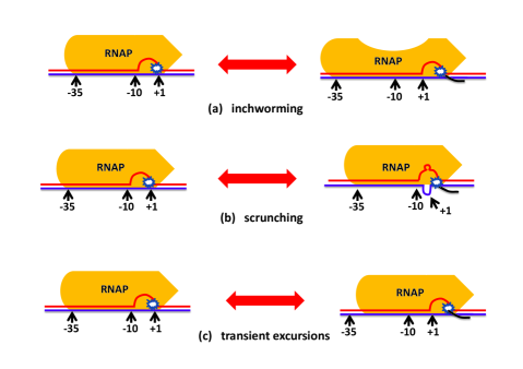
Transcription termination: role of antitermination
Termination of transcription is also a complex phenomenon and it can be regulated by intrinsic or extrinsic signals [1501, 1502]. Assisted by anti-termination factors, a RNAP may ignore a stop signal and may continue transcribing beyond the stop signal sequence.
Elongation: Brownian ratchet or power stroke?
Theoretical modelers have paid most of the attention so far on the elongation phase. Each mechao-chemical cycle in the elongation stage involves two main sub-stages: polymerization and translocation. Polymerization elongates the RNA transcript by 1 nucleotide. During translocation, the RNAP moves forward by 1 nucleotide on the dsDNA which requires unzipping the downstream DNA by 1 nucleotide and simultaneous re-annealing of the upstream DNA by 1 nucleotide. Moreover, at the same time, the RNA-DNA hybrid also moves by 1 nucleotide so that the 3’end of the RNA vacates the active site of the RNAP and the RNA-DNA hybrid opens by 1 nucleotide at the 5’-end of the RNA.
To our knowledge, one of the earliest attempts was the model developed by Jülicher and Bruinsma [1503]. One special feature of the model is that is assumes an “internal flexibility” of the RNAP itself and captures this flexibility by an elastic element that allows compression of the separation between the catalytic site and front of the RNAP. Thus, the kinetics of transcription is described in terms of two stochastic variables: the position of the catalytic site along the DNA template and the internal deformation of the polymerase. Almost simultaneously Wang et al.[1504] developed a stochastic model of transcription that included the detailed enzymatic cycle of the RNAP. It is essentially based on the Brownian ratchet mechanism of energy transduction where the binding of the NTP monomeric subunits rectify diffusion of the RNAP.
In a Brownian ratchet model of RNAP [1482, 1505, 1506, 1507] the polymerase is assumed to fluctuate back and forth between the “pre-translocated” and the “post-translocated” positions. In the absence of NTP, this motion is essentially an unbiased Brownian motion. However, when NTP binds, it rectifies fluctuations thereby biasing forward movement of the RNAP. Thus NTP would serve as a “pawl”. High quality single-molecule data [1508] as well as high-resolution structures obtained from X-ray crystallography [1509] are consistent with this Brownian ratchet mechanism and inconsistent with the power stroke mechanism. The predictive power of the Brownian ratchet mechanism has been tested more stringently [1510]. Using the parameters extracted under chemical perturbation,predictions were made, and tested, for responses to mechanical perturbations. Chemical perturbation was achieved by varying the composition of the sequence-inhomogeneous template and the concentration of the NTPs. Transcription was perturbed mechanically by applying mechanical force. Because of the sequence inhomogeneity, the rates of transitions from the pre-translocated to the post-translocated states were also sequence dependent. These rates of transitions were computed from thermodynamic considerations quantifying [1511] earlier ideas formulated qualitatively by von Hippel and collaborators [1512]. An even more elaborate Brownian ratchet mechanism has been proposed and quantified by Bar-Nahum et al. [1513]; it involves a static pawl with a asymmetric ratchet and a dynamic (reciprocating) asymmetric pawl with a symmetric ratchet. But, perhaps, not all RNAPs follow Brownian ratchet mechanism. Structural evidences have been presented in support of a power stroke mechanism for a class of RNAPs [1514]. In order to reconcile these two apparently contradictory observations and settle the controversy on the mechanism, Yu and Oster [1515] have developed a model that allow two parallel paths- one of these is based essentially on a Brownian ratchet mechanism whereas the other utilizes a power stroke. The seven states and the kinetic pathways are shown in fig.46. Approximate analytical expressions for the rates of elongation in the steady states of the process were derived separately for single-subunit RNAPs and multi-subunit RNAPs (see the supporting information of ref.[1515] for the details).
Figure NOT displayed for copyright reasons.
An alternative formulation [1516], based on the Fokker-Planck equation, also allows the possibilities of both the power stroke and Brownian rachet mechanisms by the appropriate shape of the free energy landscape. Not all kinetic models explicitly assume either the power stroke or the Brownian ratchet mechanism. Some purely kinetic models [1517, 1518, 1519] can be interpreted in either way because these assume movements of the RNAP without explicitly explaining how these movements are caused by the energy transduction mechanism. One of these is the “look-ahead” model [1518, 1519], which assumes the existence of a “look-ahead” window ahead of the catalytic site within the transcription bubble at which NTP can bind reversibly before they are covalently linked to the RNA transcript.
Pause and backtracking of RNAP: kinetics and error correction
So far in the context of elongation stage, we have discussed, only the pathway that consists of the sub-stages of polymerization and translocation. However, at each position on its template, multiple pathways are available to a real TEC. The pathways alternative to elongation include termination, pause and arrest (in backtracked positions), editing, etc. [1512]. The relative probabilities of entering into any of the available pathways depends not only on the sequence-specific interactions of the RNAP with its template DNA, but also on its interactions with the nascent RNA transcript as well as that with regulatory transcription factors.
On the basis of the duration, pauses have been divided in two classes: Of all the pauses, about 95% do not last longer than a few seconds and, therefore called “short” pause. The duration of the remaining 5% of the pauses can be in the range 20 s - 30 min and these are called “long pauses”.
The pauses can be broadly divided into two categories also on the basis of their relation with backtracking [1520]: (i) pausing without backtracking, in which only nucleotide addition is blocked, (ii) paused state following backtracking in which RNAP reverse translocates on its template by a few steps. Backtracking has been investigated by single-molecule techniques [1521, 1522, 1523] as well as in structural studies [1524, 1525]
The mechanism of pausing and backtracking as well as the effects of force on these phenomena remain controversial [1522, 1526, 1523, 1511, 1527, 1528]. According to some schools of thought, all pauses, irrespective of the duration, arise from backtracking. In contrast, adherents of alternative scenarios believe that the cause of short and long pauses are quite distinct; long pauses are associated with backtracking whereas short pauses do not necessarily need any backtracking. Stochastic models have been developed for the kinetics of backtracking [1529, 1530, 1531, 1532, 1533].
Experimentally observed transcriptional fidelity is a consequence of two-stage selection of the nucleotide dictated by the template.
Some of these models explicitly incorporate steps for proofreading by either an isolated single RNAP [1534] or by individual RNAP motors in a traffic of RNAPs [1535]. In the first stage, the complementarity of shape and Watson-Crick base pairing helps in the selection of the correct nucleotide. In spite of this selectivity, misincorporations occasionally do occur. If a misincorporation takes place, disruption of the catalytic site conformation slows down transcription thereby allowing sufficient time for activation of the exonuclease activity of the RNAP. Once the misincorporated nucleotide is cleaved a new elongation cycle begins to select the correct nucleotide. This mechanism for ensuring high transcriptional fidelity has been established by structural techniques [1536] as well as single-molecule experiments.
Suppose () denotes the position of the last transcribed nucleotide on the template. In other words, is also the length of the nascent transcript. Let () denote the position of the TEC (more specifically, the position of the catalytic site of the RNAP) relative to . In this notation, indicates that the TEC is an active state whereas backtracked states correspond to . The transcription process starts at and terminates at . Voliotis et al.[1534] defined (and ) as the probabilities for reaching the termination site , having incorporated the correct (and an incorrect) nucleotide at the position . They obtained a site-wise detailed measure of the transcriptional error by calculating where .
For a fixed , is the probability of finding the TEC at at time , having started at at time . Defining a column vector whose elements are the probabilities (), the master equations for these probabilities can be expressed in a compact notation
| (256) |
in which is the tridiagonal transition matrix. The superscript indicates that the matrix depends on the sequence of nucleotides along the nascent transcript. Note that is a binary variable: for correct transcription whereas for incorrect transcription. Thus, for a transcript of length , is a string of length , each element of which can be either 0 or 1 depending on correct or incorrect incorporation at the respective positions on the RNA transcript. However, the matrix depends only on the elements of , namely, on .
In this formulation, there are “absorbing boundaries” through which the TEC can make an exit from the template position . The absorbing boundary at corresponds to polymerization so that the catalytic site moves from to . In contrast, the absorbing boundaries at correspond to cleavage of the transcript that causes the catalytic site to move from to because of the cleavage occuring at the backtracked state . Applying a technique based on Laplace transforms, Voliotis et al.[1534, 1537] calculated , the probability of hitting the absorbing boundary at , and the corresponding mean exit time . On time scales much longer than those for elongation and cleavage of the transcript, the kinetics can be described on a coarse-grained temporal resolution in which the elongation and cleavage are captured only through the rates and , respectively. Suppose denotes the probability of finding a transcript of length , irrespective of the sequence . Voliotis et al. [1534] wrote down the master equation for where the expressions for probability flux involve and that were calculated for fixed . From this master equation, they obtained estimates of by analytical treatment.
24.1.1 Effects of RNAP-RNAP collision and RNAP traffic congestion
Two RNAPs can collide while transcribing either (i) the same gene, or (ii) two different genes. In the former case only co-directional collision is possible whereas in the latter case both co-directional and head-on collisions can take place depending on the relative position of the two genes.
Two RNAPs transcribing the same gene
While transcribing the same gene simultaneously, the two RNAPs would move on the same DNA template strand and are co-directional. This situation is analogous to that of two vehicles in the same lane of a highway where both the vehicles are supposed to enter and exit the traffic at the same entry and exit points on this highway. In such a co-directional collision, does the trailing polymerase get obstructed by the leading polymerase or does the leading polymerase get pushed from behind?
The leading RNAP may stall either because of backtracking or because of “roadblocks” created by other DNA-binding proteins. In both these situations, the co-directional trailing RNAP can rescue the stalled leading RNAP by “pushing” it forward from behind [1538, 1539, 1540]. Two distinct underlying mechanisms can manifest as “pushing” by the trailing RNAP [1541]- in the first, the push exerted by the trailing RNAP on the leading stalled RNAP is a “power stroke”; in the second, the leading stalled RNAP resumes transcription by thermal fluctuation just when the trailing one reaches it from behind thereby rectifying the backward movement of the leading RNAP by a “Brownian ratchet” mechanism. The elasticity of the TECs may give rise to other possible outcomes of RNAP-RNAP collisions. For example, if the leading RNAP is “obstructed” by a sufficiently strong barrier, the trailing RNAP can backtrack after suffering collision with it [1542]. Moreover, the stalled leading TEC must be at least 20 bp away from the promoter so that the trailing TEC can get stabilized before encountering the stalled TEC in front of it and restart transcription by the leading TEC [1543].
Two RNAPs transcribing two different genes
Next we consider the more complex situation where the two interacting RNAPs transcribe two different genes. Their interaction can cause transcriptional interference (TI). TI is defined as [1544, 1545, 1546, 1547, 1548] the “suppressive influence of one transcriptional process, directly and in cis on a second transcriptional process”. TI can occur when both the genes are on the same DNA strand so that both the RNAPs move from the 3’ to 5’ end of the template DNA strand. Anti-sense RNA transcripts are synthesized by RNAPs that translocate from the 3’ to the 5’ end of the (+)DNA strand (i.e., codingDNA strand).
Figure NOT displayed for copyright reasons.
The RNAP transcribing one gene can interfere with the initiation,
or elongation, or termination of transcription of another
neighbouring gene. The possibility of a transcriptional interference
between two neighboring genes and the relative direction of
approach of the two RNAPs is decided by the arrangement of the
interfering promoters. The three alternative arrangements
(see fig.47) are named as follows
[1544, 1545, 1549, 1550]:
(i) Convergent promoters (fig.47(b)):
the RNAPs collide “head-on”.
(ii) Tandem promoters (fig.47(a)):
the RNAPs are co-directional; the collision takes place between the
front edge of the trailing RNAP and the rear end of the leading RNAP.
(iii) Divergent (overlapping) promoters (fig.47(c)):
Except for the initial mutual hindrance in starting their journey on
their respective tracks, the RNAPs do not interact once they depart
from the sites of initiation and start elongating their own transcripts.
Based on the stage of transcription, one can envisage four
different types of interference and the corresponding possible outcomes:
(I) Promoter competition: Occupation of one promoter by a RNAP
hinders the occupation of the promoter by the other RNAP if the
promoters are overlapping (divergent). Thus, initiation of
one transcription interferes with the initiation of the other.
Unless influenced by other regulatory molecules, only one of the
two RNAPs succeeds in initiating transcription at a time. The
winner of the competition could be decided randomly if their binding
affinities are comparable. The overall effect is either systematic or
random suppression of the expression of one or both of the genes.
(II) Occlution: A RNAP cannot even initiate transcription,
if the promoter is occluded, at least temporarily, because of the
occupation of the site by another RNAP that is already elongating
its transcript. This phenomenon can occur for both tandem and
convergent promoters. If the occupying RNAP transcribes at a normal
rate, the occlution effect is marginal because it vacates the
promoter site of the other RNAP within seconds. However, if the
occupying RNAP is in a stalled state because of backtracking, it can
delay initiation of transcription of the other gene for a long time
[1551].
But, no real collision of two RNAPs takes place in this case.
(III) Sitting duck mechanism: If one of the two RNAPs in
still in the stage of transcription initiation (and yet to begin
transcript elongation), it is regarded as a “sitting duck” that
can get “hit” by another RNAP that is already in the stage of
elongation of its transcript. This mechanism of TI is significant
when the two promoters are sufficiently close but do not overlap.
The most likely outcome is that the sitting duck is dislodged from
the DNA template.
(IV) Traffic collision: If both the RNAPs are engaged in the
elongation of their respective transcripts, a “head-on” collision
between their TECs is possible if the promoters are convergent.
Alternatively, a co-directional collision of the two RNAPs is
also possible for tandem promoters if the trailing RNAP transcribes at
a faster rate than that of the leading RNAP. Strong TI can be caused
by such collision if the distance between the two promoters is
sufficiently large so that both the RNAPs are engaged in elongating
their respective transcripts when they collide. If one of the
RNAPs bind strongly to its template while the other binds weakly,
the strongly bound RNAP acts as a “roadblock” for the weakly
bound RNAP. The outcome of the collision could be any of the
following depending on the specific organism and the particular
gene:
(i) Either or both of the RNAPs can stall and/or backtrack.
(ii) Either or both of the RNAPs can get dislodged from the template
causing premature abortive termination of the corresponding
transcriptions.
(iii) In case of “head-on” collision, the two RNAPs can simply pass
each other just like two cars on two adjoining central lanes meant for
oppositely moving vehicular traffic [1552].
(iv) In case of “co-directional” collision, the stalled leading RNAP
can restart transcription by the push of the trailing RNAP.
Based on the existing mathematical model [1553], the
following predictions have been made:
(i) Occlusion is strong and dominating when the interfering promoter
is very strong.
(ii) Collision dominates TI if the interfering promoter is
strong or if the convergent promoters are sufficiently far apart
(typically bp).
(iii) If the interfering promoter is not strong enough or if the
convergent promoters are not far enough from each other, the
sitting duck mechanism is expected to dominate TI.
Many RNAPs transcribing the same gene: traffic congestion
Traffic-like collective movement of many RNAPs during transcription of a gene and the effects of traffic congestion on the rate of transcription has been studied theoretically [1517, 1554, 1555, 1556]. The effects of RNAP traffic congestions on the pausing and backtracking of RNAPs and the consequent implications for transcriptional proofreading have also been investigated theoretically by Sahoo and Klumpp [1535]. The theoretical framework of this work has many similarities with that formulated by Voliotis et al.[1534] for the special case of nucleolytic proofreading by a single isolated RNAP via backtracking.
24.1.2 Primase: a unique DdRP
DdDP cannot begin polymerization of a polynucleotide from scratch. First, a DNA primase [1557, 1558, 1559, 1560, 1561] polymerizes a short RNA primer using the DNA template. Just like a RNAP, a primase identifies its binding site on the template DNA by a particular sequence. This initiation is followed by the elongation of the RNA primer. Thus, a primase in a special type of DdRP. One of the challenging questions is: what determines the length of the primer that the primase must polymerize? Once the primer reaches that length, the primase disengages and the DNAP takes over adding nucleotides to the primer thereby continuing DNA replication. On one of two template strands exposed by the unzipping of the dsDNA by a helicase, the priming event occurs only once in the beginning of DNA replication. But, on the other template strand priming occurs repeatedly because on this template DNA replication takes place in discontinuous segments each of which requires separate priming. The mechanism of the coordination between the primase and DNAPs on the two template strands will be discussed in the next subsection.
24.2 Replication by DNAP: a DdDP
In this section we study the kinetics of DNAP, a DdDP, during replication of DNA [1562]. The chromosome replication cycle can be broadly divided into a few distinct stages [1563] that are more complex than the stages of transcription. Therefore, we present the kinetic processes in the order of increasing complexity, rather than the actual sequence of the stages of replication of the whole genome.
24.2.1 Coordination of elongation and error correction by a single DdDP: speed and fidelity
In their pioneering work on DNAP, Wuite et al.[1564] a ssDNA molecule, that served as the template, was subjected to tension by holding it with a micro pipette at one end and an optical trap on the other. Almost simultaneously, Maier et al.[1565] carried out a similar experiment on a different DNAP where a magnetic trap was used, instead of an optical trap. In both these experiments, the DNAP converted the ssDNA into a dsDNA by polymerizing a strand that is complementary to the template. An interesting feature of the data is the nonmonotonic variation of the average rate of replication with the tension ; exhibits a maximum [1564, 1565].
The experimental data were interpreted quantitatively in terms of a phenomenological model [1564, 1565] based on a thermally activated rate-limiting step. The rate constants and , in the presence and absence, respectively, of the tension were assumed to be related by , where is the force-induced change in the free energy barrier . The barrier was assumed to have the form
| (257) |
where the first term on the right hand side is the enthalpic contribution while the second term is the entropic contribution to . and are the measured (in different experiments) extensions per base of the ssDNA and dsDNA strands, respectively, at force . Wuite et al.[1564] evaluated the from
| (258) |
A comparison of the force-extension curves of ssdNA and dsDNA explains the observed trend of variation of . For forces , dsDNA contour length is longer than that of ssDNA whereas for the ssDNA is longer; the magnitude of the crossover length is about 5 pN. DNAP induces this change in length as it converts a ssDNA into a dsDNA. Therefore, for the DNAP is assisted by the external tension whereas for its operation is opposed by the applied tension .
Note that and are the contributions per base to the end-to-end net extension of the entire ssDNA and dsDNA chains, respectively. Each of these chains, typically, consists of thousands of nucleotides. Thus, this phenomenological model [1564, 1565] implicitly assumes that the global force-extension behavior of “bare” long ssDNA and dsDNA chains, rather than their local interactions with the DNAP, is the dominant cause of the observed -dependence of the rate of DNA replication. Therefore, this model was later named as the “global” model. The effect of the DNAP enters into the results of this model only through the parameter , which denotes the number of ssDNA bases that get converted to dsDNA in each polymerization reaction catalyzed by the DNAP. It also ignores the fact that at the active site of DNAP the ss and ds segments of the DNA are far from collinear. The resulting torque generated by the tension has important energetic implications which the global model ignored.
As an alternative to these “global” models, a “local” model was developed by Goel et al. [1566, 1567] to calculate for a quantitative interpretation of the same experimental observations. This model focusses only on the nucleotides in the immediate vicinity of the active site of the DNAP.
Both the global and local models described above assume that although the rate of the rate-limiting step is altered by the tension , none of the non-rate-limiting steps become rate-limiting in this process. An atomistic model, that does not need to make any of these assumptions, was developed later by Andricioaei et al. [1568] to calculate the force-dependent barrier. This “restricted-cone local model” [1568] correctly excludes many of the orientations of the DNA because of steric constraints imposed by the DNAP. All the models described above can account for the qualitative features, particularly the nonmonotonicity, of the variation of the rate of replication with increasing tension applied on the template DNA.
In an alternative approach, the force-dependence of the replication rate was interpreted by Venkataramani and Radhakrishnan [1569] from a different dynamical perspective in terms of a subtle interplay of fast motions of the catalytic site and the slow delocalized modes of the DNA-DNAP complex. However, their analysis breaks down because of anharmonic effects at strong forces. Therefore, they could present results for applied tensions upto a maximum of pN.
Application of external tension on the template DNA strand is just one of the many possible ways to control the rate of DNA replication. Secondary structures of the template, DNA-bound ligands and sequence inhomogeneities can also have significant effect on replication speed. Since replication is interrupted by pauses caused by the heterogeneous sequence of the template, the average replication rate extracted from ensemble measurements does not reflect the intrinsic “speed limit” of the DNAP motor. In a single-molecule study [1570], that had sufficient spatial and temporal resolutions, the paused and burst phases of replication were separated to measure the true intrinsic “speed limit” of a DNAP.
A DdDP is a dual-purpose enzyme that plays two opposite roles in two different circumstances during DNA replication. It plays its normal role as a polymerase catalyzing the elongation of a new DNA molecule. However, it can switch its role to that of a exonuclease catalyzing the shortening of the nascent DNA by excision of the nucleotide at the growing tip of the elongating DNA [1571, 1572, 1573, 1574]. The two distinct sites where, respectively, polymerization (pol) and exonuclease (exo) reactions are catalyzed, are separated by 3-4 nm on the DNAP [1575, 1576]. Once a misincorporation of a nucleotide takes place, the DNA is transferred from the pol-site to the exo-site. After excision of the wrong nucleotide from its growing tip, the trimmed DNA is returned to pol-site for resuming its elongation. The elongation and cleavage reactions are thus coupled by the forward and reverse transfers of the DNA between the pol- and exo-sites of the DNAP. “Exo-deficient” mutants and “transfer-deficient” mutants have been used in single-molecule experiments to understand the interplay of exonuclease and strand transfer processes on the platform of a single DdDP [1576, 1577]. By varying the tension applied on the template strand, the kinetics of the pol-exo transfer has been probed.
Very recently Sharma and Chowdhury [1578] have extended the earlier kinetic models to develop a more detailed Markov model of DNA replication that captures, in addition to the pol and exo activities, also the palm closing and palm opening conformational transitions. This model accounts for the observed nonmonotonic variation of the average rate of replication with increasing tension on the template strand. Going beyond the earlier theoretical treatments of DNA replication, Sharma and Chowdhury [1578] have also defined, and calculated, 9 distinct conditional dwell times of the DNAP motor.
24.2.2 Replisome: coordination of machines within a machine
Unlike RNAP, the DNAP is not capable of helicase activity. Therefore, ahead of the DNAP, a helicase progressively unzips the dsDNA thereby exposing the two single strands of DNA which serve as the templates for DNA replication. For the processive translocation of a DNAP on its template, it needs to be clamped with a ring-like “DNA clamp”, which is assembled by a “clamp loader” in a ATP-dependent manner [1579, 1580, 1581, 1582, 1583, 1584]. DNAP cannot initiate replication on its own and requires priming by another enzyme called primase, which we have already described above. Thus, DdDPs alone cannot replicate the genome; together with DNA clamp and clamp loader, DNA helicase and primase, it forms a large multi-component complex machinery which is often referred to as the replisome [1585, 1586, 1587, 1588, 1589, 1590, 1591, 1592, 1593, 1594, 1595, 1596, 1597, 1598, 1599, 1600, 1601]. How does the DNAP coordinate its motion with that of the helicase? How does a primase and a DNAP coordinate their operation so that when primase stops further elongation of the RNA primer and disengages itself, the DNAP takes charge and begins polymerization of a DNA strand? The spatio-temporal coordination of the operation of the different components of the replisome during DNA replication is the most interesting aspect of its operational mechanism.
24.2.3 Coordination of two replisomes at a single fork
Two DdDPs have to replicate two complementary strands of DNA. However,
each DdDP is capable of translocating only unidirectionally()
for elongating the product strand. As a result, one of the strands
(called the “leading strand”) is synthesized processively, whereas
the “lagging strand” is replicated discontinuously
(see fig.48); the “Okazaki
fragments” synthesized by this discontinuous process are then joined
together (ligated) by an enzyme called DNA ligase.
Processing of the Okazaki fragments into a continuous DNA strand
takes place in three steps catalyzed by three enzymes which are
not part of the replisome: (a) removal of the RNA primer by a
separate 5’3’ exonuclease (which is distinct from the 3’5’
exonuclease domain of the DNAP that is used for proofreading and
editing during elongation); (b) filling the gap, which is left
open by the removal of RNA primer, by a DNA polymerase; (c) sealing
the nick by a DNA ligase.
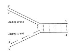
How are the replications of the leading and lagging strands maintain tight coordination as the replication fork moves forward? Do the DNAPs on the two strands polymerize at the same average rate? If so, does the DNAP on the leading strand pause at the replication fork till the DNAP on the lagging-strand catches up again? In such a scenario, can any component of the replisome, e.g., the primase, or helicase, operate effectively as a “brake” preventing the leading-strand synthesis from outpacing the lagging-strand synthesis of DNA [1600]? Alternatively, does the DNAP on the lagging strand polymerize at a faster rate than that on the leading strand so as to make up for the time lost in the priming and in re-starting DNA elongation thereby enabling it to catch up the DNAP on the leading strand [1601]?
24.2.4 Traffic rules for replication forks and TECs: DNAP-DNAP and DNAP-RNAP collisions
In the preceding subsubsection we have studied the coordination of the two DNAPs at a single replication fork. Now we review coordination of multiple forks during genome-wide replication. Moreover, we review some of the common causes for a temporary pause or permanent stall of a replication fork by either damage of the track or by the present of “blockage” on its way [1602].
Coordination of replication and transcription: DNAP-RNAP collision
Once replication of the genome begins, the replication forks may encounter TECs on the way. Therefore, for an orderly execution of replication and transcription, either (a) their progress must be coordinated in such a way as to avoid possibilities of collision, or (b) there must be a mechanism for resolving such collisions [1603, 1604, 1605, 1606, 1607, 1608]. One could imagine that, in addition to the direct physical contact between a DNAP and a RNAP in a collision, topological changes in the track induced by one polymerase can affect the movement of the other. Moreover, a RNAP may find itself stalled in a backtracked state while a DNAP approaches it either from front or from behind. The outcome of the collision in such a situation need not be the same as in cases where the RNAP is actively transcribing a gene. Furthermore, if a gene is being transcribed by several RNAPs simultaneously while a replication fork approaches that segment of DNA, the replication fork may have to deal with multiple RNAPs sequentially.
Let us begin with the DNAP-RNAP encounter during their co-directional translocation. Suppose the DNAP, the faster of the two, approaches the RNAP from behind. The three alternative outcomes of such a collision are as follows: (a) the DNAP dislodges the RNAP from the template, thereby aborting transcription, and goes ahead with replication; (b) the DNAP slows down so as to avert collision; in this case the maximum rate of replication can equal that of transcription until RNAP detaches from the termination site after completing transcription; (c) the DNAP passes (or bypasses) the RNAP without dislodging it so that both the polymerases can come out of the encounter unscathed and continue their respective tasks.
Since both DNAP and RNAP move from 3’-to-5’ direction on the template DNA, they must move on the complementary strands while moving in the opposite directions on the same duplex DNA. Therefore, at first sight, a head-on collision between a DNAP and a RNAP, while approaching each other on the same duplex DNA, may seem unlikely. However, each DNAP on the leading strand is accompanied by the other members of the replisome and another DNAP on the lagging strand. Thus, although the DNAP on the leading strand would not collide with the RNAP approaching it from its front, the other proteins at the replication fork would certainly suffer a head-on collision with the RNAP.
To our knowledge, the first systematic survey of the literature on the traffic rules of DNAP and RNAP motors was carried out by Brewer [1603]. However, it was the experiments performed, a few years later, by Alberts and collaborators, both on co-directional [1609, 1610] and head-on collisions [1611] between DNAP and RNAP that opened up a new frontier of research. The general concensus now is that the head-on collisions affect replication more adversely than co-directional collision. Replication fork stalling [1612, 1613], which can arise also from the interactions of the fork with non-RNAP proteins, can have severe consequences, e.g., genomic instability. However, several other proteins may play roles of regulators that either reduce the chances of fork stalling or restart stalled fork [1614, 1605, 1615]. To my knowledge, no serious effort has been made till now to develop kinetic models of heterogeneous traffic of DNAPs and RNAPs, incorporating possibilities of both co-directional and head-on collisions described above.
24.2.5 Initiation and termination of replication: where, which, how and when?
The mechanism of initiation [1616] and termination [1617] of replication are quite different from those of transcription. In bacteria, there is a single location, called the origin of replication (and denoted by OriC), from where replication fork propagates bidirectionally (i.e., in both the clockwise and counter-clockwise directions on the circular dsDNA) [1562, 1618]. The replication is completed when the two forks meet head-on. Naively, one might think that in eukaryotes the replication of the mitochondrial DNA (mtDNA) and that of the chloroplast DNA (cpDNA) might be similar to that of bacterial DNA. However, the mechanism of replication of mtDNA remains controversial [1619, 1620, 1621, 1622, 1623, 1624] and that of cpDNA remain shrouded in mystery [1625]. The most striking feature of replication of mammalian mtDNA is that the leading and lagging strands are replicated from separate origins designated as (for the heavy, or leading strand) and (for the light, or lagging strand). Moreover, the replication initiation of the two strands are also asynchronous; the synthesis of the lagging strand begins much later than that of the leading strand. The polymerase , the DdDP that drives replication of mtDNA, is assisted by a mitochondrial hexameric helicase called TWINKLE [1626].
In comparison with DNA replication in bacteria, that in eukaryotes seem to be much more complex [1627, 1628, 1629, 1630, 1631, 1632, 1633, 1634, 1635, 1636, 1637]. First, the length of the DNA in a eukaryotic cell is so long that if it had a single origin of replication, a few years (typically, 5 years for a human cell) would be needed to complete replication once. To circumvent this problem, most of the eukaryotic cells initiate replication at many sites (typically, thousands of sites in a human cell) so that replication can be completed in minutes (in embryos) to hours (in somatic cells). So, the fundamental questions are (i) where are these potential origins of replication located, (ii) which of these potential origins actually get activated to begin replication (i.e., “fire”), (iii) how, i.e., by what kind of molecular signaling or interaction, does this “firing” take place, and (iv) when, i.e., in which type of temporal sequence, do the origins “fire”? How does the spatio-temporal organization of replication initiation and progress ensure that no segment is left unreplicated at the end and no segment is replicated more than once? These fundamental questions have been addressed by studying the spatio-temporal pattern of firing of origins and the fork propagation with several ingeneous experimental techniques [1638, 1639].
“License” to “fire”
The mechanism of genome wide DNA replication ensures that no segment is replicated more than once in a cell cycle. In other words, the replication origins get “licence” to “fire” once, and only once, in a cell cycle [1640, 1641, 1642, 1643].
Where are the potential origins located: marked or unmarked?
The first fundamental questions is: where are the potential origins of replication located? Are these potential origins equispaced or distributed randomly along the DNA? Are these chemically marked on the DNA by any specific sequence? Barring a few exceptions, most eukaryotic cells randomly select many sites, irrespective of the sequence, as the potential origins of replication [1635]. A pre-replication complex (pre-RC) of macromolecules, that includes the origin recognition complex (ORC), is assembled at each selected site.
The next obvious question is: how are these potential replication sites selected, i.e., spontaneously or guided by any signal molecule(s)?
Which of the potential origins “fire” and how?
To begin with, not all the selected potential origins need to get activated (i.e., “fire”). Drawing analogy with the biblical statement of St. Mathew, this principle has been articulated in the literature [1627] as the statement “many are called but few are chosen”. So, which of the selected origins fire- are they all equally likely to fire or some are more likely than others to fire? It is now generally believed that a random fraction of the pre-RC get activated for initiation of replication.
How do the origins fire: molecular communication and interactions?
The major component of ORC is a helicase. A pre-RC is activated to a pre-initiation complex (pre-IC) by a special class of enzymes (kinase). Then, recruitment and loading of other components of the replisome, including DNAP, and the formation of the two replication forks are followed by priming.
When do the origins fire: simultaneously, in ordered sequence or randomly?
What is the temporal sequence in which the origins get activated, (i.e., they “fire”)- simultaneously, or in any ordered sequence, or random sequence [1644]? There are strong evidences from experiments that not all the selected potential origins fire simultaneously. Instead, they fire in a random sequence; however, each origin that fires can fire once, and only once, in a cell cycle.
But this random firing could give rise to another problem [1635, 1631, 1632]: there is non-zero probability that a pair of activated sites may be separated by a very large gap which would take enormously long time to get replicated. To speed up the process, eukaryotic cells have a smart strategy. The rate of firing itself keeps increasing with the passage of time. Consequently, the longer a large gap persists the higher is the probability that some other pre-RC located in this gap would fire.
It is obvious that not all the selected potential origins would get an opportunity to fire in the cell cycle in which they were selected. Why does an eukaryotic cell opt for such a redundancy? Perhaps, the cell has its back-up plans- in case any running fork hits an unexpected barrier and stalls, its pending job can be completed by one (or more) of the back-up origins that fire later in the sequence.
Thus, during a specific cell cycle the potential origins of replication may have two alternative fates: (a) to “fire” and get replicated (called “active” replication), or (b) not to “fire” and get replicated when a fork initiated at some other origin passes through it (called “passive” replication). By monitoring this process over sufficiently large number of cell cycles, one can measure the “firing efficiency” of a specific origin [1645]. In general, the firing efficiency is not expected to be uniform across all origins.
24.2.6 Genome-wide replication: analogy with nucleation, growth and coalescence
In order to develop a theoretical description of genome-wide replication, let us recall a classic problem in non-equilibrium statistical mechanics: nucleation of ordered crystalline solid in a metastable supercooled liquid, followed by growth of the crystallites and their coalescence. “Crystals” nucleate by thermally activated process. However, only those crystalline domains whose initial size is larger than a critical size grow, others simply shrink and disappear. If two (or more) growing crystalline domains impinge on one another, they coalesce to form a single crystal that can, then, continue to grow further. For nucleation, growth and coalescence of ordered crystalline domains, the Kolmogorov-Johnson-Mehl-Avrami (1D-KJMA) model provides many analytical results in one-dimension.
Stochastic models for the genome-wide DNA replication has been developed by several research groups (see, for example, ref.[1646]). A formal mapping of the whole genome replication and the 1D-KJMA was identified a few years ago and fully utilized for quantitative analysis [1647, 1648, 1649, 1650, 1651, 1652, 1653] (see table 11).
| 1D-KJMA | Genome duplication |
|---|---|
| Crystalling solid | Replicated region |
| Metastable liquid | Unreplicated region |
| Nucleation | Firing |
| Crystal growth | Replication progress |
| Coalescence of growing crystals | Meeting of replicated regions |
The increasing rate of firing would correspond to a increasing rate of nucleation in the KJMA-type models [1654, 1655]. However, the original 1D-KJMA model assumed a stationary (i.e., time-independent) rate of nucleation . Therefore, to adapt the nucleation-type theories for describing firing of the potential origins of replication, the 1D-KJMA theory had to be extended by allowing the rate to increase with time [1647, 1648, 1649, 1650, 1651, 1652, 1653].
The rate at which the total fraction of the replicated genome increases with time quantifies the rapidity of the genome duplication process. However, the evolving spatial pattern is characterized in more detail by the distributions of (a) the sizes of the replicated segments, (b) the spatial gap between the replicated segments, (c) the distance between the centers of two neighboring replicated segments, etc. The effects of defects on the kinetics has also been investigated within the framework of this formalism [1656].
The main quantity calculated in the KJMA-based theory is the local initiation rate . On the other hand, experimental data on genome-wide replication provides information on the unreplicated fraction . In most of the early attempts in testing the predictions of the KJMA-based theory, curve-fitting strategies were used to estimate from the genome-wide replication timing data. In a recent work Baker et al. [1657] have analytically inverted the KJMA-based model deriving the expression
| (259) |
where is the d’Alembertial operator. The equation (259) can be used to extract from the experimental data.
25 Ribosome motor translating mRNA track: template-directed polymerization of proteins
Ribosome, one of the largest and most sophisticated macromolecular machines within the cell, polymerizes polypeptides using a mRNA as the corresponding template [16, 1658, 1659, 1660, 1661, 1662, 1663, 1664, 1665]. Although it works effectively as a polymerase, it differs from the polynucleotide polymerases in two important respects: (i) it is a ribonucleoprotein whereas polynucleotide polymerases are proteins, (ii) the track is a mRNA strand, rather than DNA, and the step size is 3 nucleotides, instead of a single-nuceotide step-size of polymerases, and (iiii) it “translates”, instead of replicating or transcribing, the genetic message.
A critical analysis of the free energy cost of protein synthesis was initiated, to my knowledge, by Chetverin and Spirin [1784]. In each successfully completed mechano-chemical cycle of a ribosome two molecules of guanosine triphosphate (GTP) are hydrolyzed into guanosine diphosphate (GDP). Moreover, one of the steps of this cycle needs the assistance of specifically prepared accessory molecular assembly (aa-tRNA) whose prior preparation also involves hydrolysis of a molecule of ATP. Because of these energy-consuming steps involved in the operation of a ribosome, it is regarded as a molecular motor [1673]. It has been argued [1660] that the the energy of the chemical bond between the amino acid and tRNA is later used by the ribosome for forming a peptide bond between this amino acid and the nascent polypeptide. Just like RNAP (and unlike DNAP), ribosome is capable of helicase activity. There are strong indications [1666] that it uses two active mechanisms for unwinding mRNA during translation.
A ribosome is not merely a “protein-making motor protein” [1672] but it serves as a “mobile workshop” which provides a platform where a coordinated action of many tools take place for the selection of the appropriate subunits and for linking them to synthesize each of the proteins. As this mobile workshop moves along the “assembly line” (mRNA), new subunits (amino-acids) are brought to it by the “workers” (tRNA molecules).
25.1 Composition and structure of a single ribosome and accessory devices
The mechanisms of ribosomes in bacteria as well as those of the cytoplasmic and organellar ribosomes [1667, 1668, 1669, 1670, 1671] in eukaryotes have lot of similarities, in spite of differences in the details of their composition and kinetics. Numerical values of some of the parameters that characterize the physical properties of a typical ribosome have been listed by Moore (see table 2 of ref.[1665]).
Even in the simplest organisms like single-cell bacteria, a ribosome is composed of few rRNA molecules as well as several varieties of protein molecules. The reason for the complexity of its composition and structure can be understood by studying its possible origin and evolution over billions of years [1674].
The structure of both bacterial and eukaryotic ribosomes have been revealed by extensive detailed investigation over several years by a combination of X-ray diffraction, cryo-electron microscopy, etc. [1675, 1676, 1677, 1678, 1679, 1680, 1681, 1682, 1683, 1684, 1685, 1686, 1687, 1688, 1689, 1690]. For this achievement, V. Ramakrishnan, T.A. Steitz and A. Yonath shared the Nobel prize in chemistry in 2009 [1684, 1678, 1681]. For many years the mechano-chemical kinetics of ribosomes have been investigated by studying bulk samples with biochemical analysis as well as the structural probes mentioned above. Only in the last few years, it has been possible to observe translation by single isolated ribosome in-vitro [1691, 1692, 1693, 1694, 1695, 1696, 1697, 1698, 1699, 1700, 1701, 1702, 1703, 1704, 1705]. Very recently Sanbonmatsu [1706] has presented an excellent review of the theoretical and computational studies of ribosome.
25.1.1 Molecular composition and structural design of a ribosome
Ribosomes found in nature can be broadly divided into two classes: (i) prokaryotic S ribosomes, and (ii) eukaryotic S ribosomes; the numbers and refer to their sedimentation rates in the Svedberg (S) units. There are separate channels in the ribosome for the passage of the template mRNA and the nascent polypeptide. In the earliest electron microscopy the prokaryotic and eukaryotic ribosomes appeared to be approximately spherical particles of typical diameters in the ranges nm and nm, respectively.
Large and small subunits of a ribosome
In the earliest electron micrographs of ribosome a visible groove was found to divide each ribosome into two unequal parts; the larger and the smaller parts are called, for obvious reasons, large and small subunit, respectively. The sizes of the large and small subunits of the S ribosome are S and S respectively, whereas those of the S ribosome are S and S, respectively. The two subunits of a ribosome interact directly via “intersubunit bridges” [1707].
The small subunit assists in the decoding of the genetic message by mediating the base-pairing interaction between the tRNA and the template mRNA. But, the actual polymerization of the polypeptide takes place at a site, called peptidyl transferase center, that is located in the large subunit. These operations of the two subunits are coordinated by a L-shaped adapter molecule called tRNA.
tRNA and amino-acyl tRNA synthetase
The tRNA molecules are sufficiently long so that their two ends can interact with the two subunits simultaneously. The intersubunit space is large enough to accomodate just three tRNA molecules which can bind, at a time, with the three binding sites designated as E, P and A. Moreover, the shape of the intersubunit space is such that it allows easy passage of the L-shaped tRNA molecules. The end which carries the amino acid interacts with the large subunit while the other end, where the anticodon is located, interacts with the codon on the mRNA located on the small subunit. If the mismatch between the codon and anticodon is limited to just one codon, the tRNA is called near cognate whereas mismatch of larger number of codon-anticodon pairs occurs if the tRNA is non-cognate. Aminoacyl tRNA synthetase (aa-tRNAsynth) “charges” a tRNA molecule with an amino acid. [1708, 1709, 1722, 1710].
Elongation factors, initiation factors, release factors and NTP hydrolysis
Elongation factors (EF), which are themselves proteins, play important roles in the control of the major steps in each elongation cycle of a ribosome. Both EF-Tu and EF-G are GTPase. EF-Tu is a key player in the selection of cognate tRNA. Similarly, elongation factor G (EF-G) coordinates the orchestrated movements of the tRNA molecules within the ribosome with that of the ribosome along its mRNA track. As the name suggests, initiation factors (IF) are proteins that facilitate the steps involves in translation initiation [1716]. The ribosome recycling factor [791] plays an important role in the dissociation of the large and small subunits of a ribosome [792].
25.2 Polypeptide elongation by a single ribosome: speed versus fidelity
A ribosome covers about 30 nucleotides on the mRNA track. But, it is neither a hard sphere not a hard rod. It undergoes several functionally important conformational changes during each cycle [1717, 1687, 1718, 1719] which can be described quantitatively as the conformational kinetics of the ribosome in an energy landscape [1720].
During the elongation stage, while translating a codon on the mRNA template, the three major steps in the mechano-chemical cycle of a ribosome are as follows [1721]: In the first, based on matching the codon with the anticodon on the incoming aa-tRNA, the ribosome selects the correct amino acid monomer that, according to the genetic code, corresponds to this codon [1722]. Next, it catalyzes the chemical reaction responsible for the formation of the peptide bond between the nascent polypeptide and the newly recruited amino acid resulting in the elongation of the polypeptide. Final step of the cycle is translocation at the end of which the ribosome finds itself at the next codon and is ready to begin the next cycle.
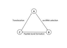
Clearly, the 3-state cycle sketched in fig.49 is an oversimplified description of the mechano-chemical kinetics of a ribosome during the elongation stage. It is inadequate to account for most of the phenomena which answer the questions listed above. We’ll see in this section that at least two of the three steps in fig.49 consist of important sub-steps. Moreover, the aa-tRNA selected (erroneously) by the ribosome may not be the correct (cognate) tRNA. Rejection of such non-cognate and near-cognate tRNAs by the process of kinetic proofreading leads to an alternative branch completion of which ends up in a futile cycle.
25.2.1 Selection of amino-acid: two steps and kinetic proofreading
Selection of the amino-acid consists of a series of steps at least two of which have major implications in optimization of translational speed and accuracy [1723, 1724, 1725, 1726, 1727, 1728, 1729]. The ternary complex consisting of aa-tRNA, EF-Tu and GTP enters the ribosome and forms a labile complex with the ribosome. In the first major step non-cognate tRNA are ejected from the ribosome because of codon-anticodon mismatch. This step exploits mainly the difference between the free-energies of binding of cognate and non-cognate tRNAs. However, this difference is inadequate to discriminate between cognate and near-cognate tRNAs. In the next major step, EF-Tu gets activated and it hydrolyzes GTP. The release of inorganic phosphate induces a change of conformation of EF-Tu because of which EF-Tu loses its affinity for the aa-tRNA. The cognate tRNA, released from the grip of EF-Tu now moves to the binding site P; alternatively, at this stage, the tRNA gets rejected by the ribosome if it is near-cognate (or non-cognate). Kinetic proofreading takes place in the second step which involves GTP hydrolysis [1731]. For a detailed discussion on the thermodynamics of the interaction between EF-Tu and aa-tRNA, see ref.[1730]. How is information on the correctness/incorrectness of the codon-anticodon matching on the small subunit transmitted to the EF-Tu and to the large subunit where the aa-tRNA contributes the amino acid to the elongating protein? Models based on alternative pathways for signal transmission have been proposed [1732, 1733, 1734, 1735]. Codon-recognition by itself may not be sufficient for stimulating the GTPase activity of EF-Tu [1733]; successful mechanical distortion of the tRNA by the ribosome seems to be necessary for sending the required signal on the codon-anticodom matching to the EF-Tu GTPase [1734]. Action of tRNA as a “molecular spring” in both decoding mRNA and translocation are well documented [1736, 1737].
25.2.2 Peptide bond formation: peptidyl transfer
The tRNA molecule that has donated the last amino acid monomer to the nascent polypeptide and to which the growing end nascent polypeptide remains bound is called the peptidyl-tRNA. Throughout the elongation stage, the ribosome retains the peptidyl-RNA in the intersubunit region. As long as the freshly arrived aa-tRNA at the A site goes through all the identity checks by the ribosome’s quality control system, the peptidyl-tRNA remains bound to the P site. Once the aa-tRNA at the A site is passed by the proofreading system, the ribosome catalyzes the peptidyl transferase reaction whereby the nascent polypeptide is transferred to the aa-tRNA by the formation of a new peptide bond between its amino-acid cargo and the nascent polypeptide.
25.2.3 Translocation: two steps of a Brownian ratchet?
In the late 1960s, Bretscher [1756] and Spirin [1757] independently proposed a concept of “locking-unlocking” [1661, 1662, 1663] of a macromolecular complex that should be applicable also to ribosomes. The complex was assumed to oscillate between locked (closed) and unlocked (open) states. In the unlocked state it accepts or releases substrates (including other ligands), moves ligands inside the complex, and releases products (and other ligands). In the locked state ligands and subatrates remain practically immobile and chemical reactions take place. The system can have more than one locked and unlocked states. The currently accepted mechano-chemical cycle of ribosomes can now be interpreted in terms of the locking-unlocking concept [1661]. The entry of the aa-tRNA and rejection of non-cognate tRNA are possible in the unlocked states whereas the peptidyl tranfer reaction requires a locked state [1758]. Completion of this reaction causes unlocking so that translocation process can begin.
Immediately after the peptidyl transferase reaction is completed, the ribosome is in the pre-translocational state in which the P site remains occupied by the deacylated tRNA while the peptidyl-tRNA is located at the A site. Before translating the next codon, the following processes must take place so that the system finds itself in the initial state of the next elongation cycle: (i) the deacylated tRNA must move from the P site to the E site while the peptidyl-tRNA moves from the A site to the P site, and (ii) the ribosome moves forward, along its mRNA track, so that the next codon is exposed to its A site. Thus, the transition to this post-translocational state from the pre-translational state involves coupled movements of two species of RNA: forward movement of the tRNA molecules through the inter-subunit space to their next binding sites, and a coordinated movement of the mRNA template along a groove in the small subunit [1748, 1749, 1750, 1751, 1661, 1752, 1753, 1754, 1755]. As we explain below, translocation needs the action of the GTPase EF-G. The dynamics of translocation has been investigated by several experimental techniques; the most important recent results have been obtained by a combination of the complementary techniques of smFRET and cryo-electron microscopy [1743, 1744, 1747].
Interestingly, the two ends of a tRNA do not translocate simultaneously. Keeping in mind that tRNA molecules interact with both the large and small subunits whereas the mRNA interacts with only the small subunit, the actual process of translocation can be split into two steps: (i) translocation of the tRNAs with respect to the large subunit and (ii) translocation of the mRNA and tRNA with respect to the small subunit.
First let us consider the movement of the two tRNA molecules with respect to the large subunit of the ribosome. The acceptor stems (i.e., the ends which can get aminoacylated) of the tRNAs located at the P and A sites translocate spontaneously to the E and P sites, respectively, on the large subunit while their opposite ends (anti-codon end) reside at the P and A sites on the small subunit thereby causing a transition from the “classical” P/P,A/A state to the “hybrid” E/P,P/A states, respectively [1738, 1739]. The spontaneous fluctuation of the two tRNA molecules between the classical and the hybrid states is accompanied by the rotational Brownian motion of the small subunit with respect to the large subunit [1740, 1741, 1742]; the angle of relative rotation of the two subunits is 60. The classical state of the tRNAs find themselves in the non-rotated state of the ribosome and this composite state, in modern terminology [1718], is often referred to as macro-state I (MS-I). In contrast, in the rotated state of the ribosome the tRNAs are in the hybrid state and, in the most recent terminology [1718], this composite state is denoted by MS-II. In the absence of EF-G, the ribosome fluctuates between MS-I and MS-II.
The rotational dynamics around an axis normal to the plane separating the two subunits is possible because of some key structural features of the inter-subunit bridges [1753, 1718]. The stronger rRNA-rRNA intersubunit bridges are concentrated near the axis that passes through the center while the weaker elastic bridges, where at least one ribosomal protein is involved, are located near the periphery. Why does the rotational Brownian motion of the ribosome begin only after peptidyl reaction is complete? Immediately after the peptidyl transfer the intersubunit interaction is reduced because of the deacylation of a tRNA which reduces resistance against the rotation.
The landscape scenario, that we presented in part I of this review to account for the interplay of conformational fluctuations and chemical reactions, has been adapted [1687] to develop a similar picture for the elongation cycle of translation. GTP-bound elongation factor EF-G biases the forward transition MS-I MS-II by altering the free energy landscape [1687]. This phenomenon (the completion of the step (i) of translocation) is one of the possible ways of physical realization of the Brownian ratchet mechanism. No relative motion between the small subunit and the mRNA template or that between small subunit and the anticodon end of tRNA takes takes place during the transition MS-I MS-II. Possibly, there are more states in between MS-I and MS-II and the existence of these states, discovered by cryo-electron microscopy [1745], need independent support also by other experimental techniques. On the basis of strong evidences from experiments it has been claimed that not only the translocation of the acceptor ends of the tRNAs with respect to the large subunit (i.e., the step (i) of translocation), but also that of the tRNA anticodons and the mRNA with respect to small subunit (i.e., the step (ii) of translocation) are governed by Brownian ratchet mechanisms [1746, 1686, 1687, 1743, 1747].
The above scenario of translocation on the free energy landscape, which was painted qualitatively on the basis of experimental data, has been quantified later by Xie [1759] in terms of a Langevin equation. One of the interesting quantities that Xie calculated using this theoretical model is the mean translocation time and predicted how would increase with the increasing magnitude of an externally applied load force.
What could be the role of EF-G and the GTP hydrolysis that it catalyzes? In principle, there are at least three different ways in which EF-G can accelerate translocation [1664]: (i) Binding of GTP-bound EF-G to the ribosome can stabilize the hybrid state thereby supporting partial forward movement of the tRNAs (movement on the large subunit). (ii) At least part of the free energy released by the hydrolysis of GTP catalyzed by EF-G can also be utilized to drive conformational changes of the ribosome itself. (iii) The conformational change of EF-G, caused by the GTP hydrolysis, can further bias the rotational diffusion of the two subunits with respect to each other towards the translocated final state.
Figure NOT displayed for copyright reasons.
25.2.4 Dwell time distribution and average speed of ribosome
By the term “dwell” we mean the duration of stay of a ribosome at a codon while actively translating that codon. As observed in single molecule experiments [1691, 1692, 1693, 1694, 1695, 1696, 1697, 1698, 1699, 1700, 1701, 1702, 1703, 1704, 1705]. the stochastic stepping of a ribosome is characterized by an alternating sequence of pause and translocation. The sum of the durations of a pause and the following translocation is defined as the time of a dwell of the ribosome at the corresponding codon. The codon-to-codon fluctuation in the dwell time of a ribosome arises from two different sources: (i) intrinsic fluctuations caused by the Brownian forces as well as the low of concentrations of the molecular species involved in the chemical reactions, and (ii) extrinsic fluctuations arising from the inhomogeneities of the sequence of nucleotides on the template mRNA [1761]. Because of the sequence inhomogeneity of the mRNA templates used by Wen et al. [1704], the dwell time distribution (DTD) measured in their single-molecule experiment reflects a combined effect of the intrinsic and extrinsic fluctuations on the dwell time.
The probability density of the dwell times of a ribosome, measured in single-molecule experiments [1704], does not fit a single exponential thereby indicating the existence of more than one rate-limiting steps in the mechano-chemical cycle of each ribosome. Best fit to the corresponding simulation data was achieved assuming five different rate-determining steps [1705].
We’ll now sketch a theoretical framework [446, 448] which provides an exact analytical expression for in terms of the rate constants for the individual transitions in the mechano-chemical kinetics of a single ribosome. This scheme also involves essentially five steps in each cycle during the elongation stage of translation. For the kinetic model shown in fig.50, the exact probability density of the dwell times is given by [448]
where , and are solution of the cubic equation
and are the solution of the quadratic equation
| (262) |
and and are the solution of the quadratic equation
| (263) |
For the sake of simplicity of analytical derivation of the exact expression for , this theory assumed the template mRNA to have a homogeneous sequence (i.e., all the codons of which are identical). Consequently, the expression for thus derived incorporates the effects of fluctuations that are strictly intrinsic. This model [448] envisages a scenario that is very similar to the protocol used in some single-ribosome experiments [1697] that use a mRNA with homogeneous coding sequence. The effects of mRNA degradation on the dwell time distribution (as well as the fluctuations in the protein copy number) has been reported [1762].
25.3 Initiation and termination of translation: ribosome recycling
Initiation of translation [1763, 1660, 1764, 1765, 1766, 1767, 1782, 1770, 1771, 1772] is a multi-step kinetic process and involves several initiation-factors [1773, 1774, 1775, 1781]. In this multi-step process, the large subunit joins the small subunit after the latter already forms a multi-macromolecular complex at the start codon after locating it. However, the detailed molecular mechanism of translation initiation in eukaryotes differ in several respects from those observed in prokaryotes [1764, 1772]. For example, in prokaryotes a specific sequence on the mRNA, called Shine-Delgarno sequence, assists in finding the start codon, [1763, 1765, 1766, 1770] whereas eukaryotes use a mRNA scanning mechanism [1768] to locate the start codon [1782, 1783].
One of the difficulties faced by the small subunit in binding the mRNA template at the ribosome-docking site (RDS) is that, for stability RNA molecules form hairpins utilizing complementary base-pairing. In the “stand-by model” [1773], one postulates that a ribosome can attach the mRNA and remains on a “stand-by” mode so that it can quickly occupy the RDS on the mRNA strand within the short time for which the hairpin can open spontaneously. Let us denote the small subunit and a folded (unfolded) hairpin by the symbols S and F (U), respectively. We also denote the complex formed by the small subunit with the folded and unfolded mRNA by SF and SU, respectively. The kinetics of the “stand-by model” [1773] is shown below
The ribosome-binding kinetics has been described [1781] in terms of three time-dependent variables, namely, number of RDS-exposed mRNAs, ribosome-bound mRNAs and free ribosomes. More detailed kinetic schemes of translation initiation, that take into account the influence of the initiation-factors explicitly, have also been developed to account for experimental data [1774, 1775].
For releasing the nascent polypeptide after its complete synthesis, release factors (RF) catalyze the hydrolysis of the bond that links it with the tRNA at the P site. Following release of the peptide, the large and small subunits disaasemble and then recycled.
25.4 Translational error from sources other than wrong selection
Translations errors are divided into two major categories: (a) nonsense error, and (b) missense error. Nonsense error occurs when a ribosome detaches from the mRNA template midway between start and stop codons thereby causing premature termination. In contrast, incorporation of a wrong (non-cognate or near-cognate) amino acid is a missense error.
We have already discussed missense error that can arise from an erroneous selection of the aa-tRNA because of the failure of the quality control mechanisms, particularly kinetic proofreading. In this subsection we discuss some of the other sources of translational error.
Potential sources of translational error keep lurking around during every stage of the process: (i) Error in “charging of tRNA by aminoacyl-tRNA synthetase: During the charging of a tRNA, if a wrong amino acid is loaded on it by the aa-tRNAsynthetase, it would lead to translational error in the elongation stage in spite of correct codon-anticodon matching. In order to ensure high fidelity of translation, the aa-tRNAsynthetase must have high specificity for its two substrates, namely, tRNA and amino acid. It has mechanism of proofreading for correction of possible errors [1708, 1709, 1722, 1710]. The error committed by by aa-tRNAsynthetase never exceeds once in enzymatic cycles. Interestingly, aminoacyl-tRNA synthetase and DNAP share some common mechanisms to ensure translational and replicational fidelities, respectively [1711].
(ii) Frameshift error: For polymerizing a specific protein, a ribosome initiates translation from a start codon and continues translation by reading successive adjacent codons. However, since there is no internal punctuation, the ribosome does not always succeed in faithfully maintaining the reading frame that recognizes adjacent triplets without any slippage of the reading frame. A slippage of the ribosome on its track by and nucleotides, where is an integer, is identified as +1 and -1 frameshifts, respectively [1712, 1713, 1714]. The consequence of frameshift can be regarded as translational “recoding” [1715] because the resulting polypeptide could be synthesized, in principle, by the translation of a recoded genetic message.
(iii) Stalled translation on aberrant mRNA and rescue of ribosome: As we mentioned earlier, ribosomes pause for long durations at rare codons. However, these “natural” pauses, arising from stochastic fluctuations, are distinct from “unnatural” stalls that are normally more stable. Because of transcriptional error, often aberrant mRNAs are synthesized. On such defective tracks, the ribosome can stall either prematurely at a codon (which may be a erroneously placed stop codon or any other codon) or at the 3’-end of the mRNA that lacks the stop codon. Such stalled translational complexes, which cannot resume operation, can have detrimental effect on the overall production of proteins [1761]. Cells have “mRNA surveillance” systems for monitoring mRNAs that are translated and degrade the troublesome ones [1776]. In order to rescue the ribosomes from stalled translational complexes, bacteria use a mechanism called trans-translation [1777, 1778, 1779, 1780]. This mechanism provides a pathway for degrading the mRNA template as well as the nascent polypeptide, and releasing the ribosome from such stalled translational complexes. The main role in this process is played by transfer-messenger RNA (tmRNA), an RNA molecule that shares the properties of both tRNA and mRNA. It enters the translational complex in the guise of a tRNA, accepts the nascent polypeptide. Then, switching role, it replaces the original mRNA by one segment of itself and the original mRNA is destined for degrading. Providing an alternative to the original mRNA, the tmRNA allows the ribosome to resumes translation whose main purpose then is to incorporate a specific amino acid that tags the incomplete polypeptide for degrading upon its release by the ribosome.
25.5 Polysome: traffic-like collective phenomena
25.5.1 Experimental studies: polysome profile and ribosome profile
Often many ribosomes move simultaneously on a single mRNA strand while each synthesizes a separate copy of the same protein. Obviously, at any instant the nascent polypeptides on different ribosomes have different lengths because the ribosomes are at different stages of their run from the start to the stop codon. Such a collective movement of the ribosomes on a single mRNA strand has superficial similarities with single-lane uni-directional vehicular traffic [495, 497] and is, therefore, sometimes referred to as ribosome traffic [498]. The ribosomes bound simultaneously to a single mRNA transcript are the members of a polyribosome (or, simply, polysome) [1785, 1786, 1787, 1788]
The polysome profiling technique [1789, 1790] provides the number of ribosomes bound to a mRNA, but not their individual positions where they remained “frozen” when translation was stopped by the experimental protocol. More detailed information on the numbers of ribosomes associated with specified segments of a particular mRNA can be obtained by using ribosome density mapping technique [1791] which is based on site-specific cleavage of the mRNA transcript. However, the ribosomes are not expected to be uniformly distributed on the mRNA template.
The detailed spatial distribution of the ribosomes on the mRNA template can be obtained by the most recent technique, called ribosome profiling [1792, 1793, 1794]. This technique effectively provides a “snapshot” of the ongoing translation by the actively engaged ribosomes on the mRNA template. There are three major steps in this method: (i) The ribosomes are first “frozen” at their instantaneous positions; (ii) the exposed parts of the mRNA transcripts (i.e., those segments not covered by any ribosome) are digested by RNase enzymes and, thereafter, the small ribosome “footprints” (segments protected by the ribosomes against the RNases) are collected separately; (iii) Finally, the ribosome-protected mRNA fragments thus collected are converted into DNA which are then sequenced. “Aligning” these footprints to the genome reveals the positions of the ribosomes at the instant when they were suddenly frozen.
25.5.2 Modeling polysome: spatio-temporal organization of ribosomes
Normally, collision between ribosomes and their queueing would reduce the overall rate of protein synthesis when translation is initiation- limited. Computer simulations of ribosome traffic have been carried out on a mRNA with a specially selected codon sequence near the start codon and allowing mRNA to decay at an optimum rate [1795]. In this case, the metabolic cost of mRNA breakdown is more than compensated by the simultaneous increase in translation efficiency because of reduced queueing of the ribosomes.
To my knowledge, all the theoretical models of ribosome traffic represent the mRNA as a one-dimensional lattice, where each site corresponds to a single codon. Since an individual ribosome is much larger than a single codon, the ribosomes are represented by hard rod that can cover successive codons () simultaneously. The inter-ribosome interactions are captured through hard-core mutual exclusion principle: none of codons can be covered simultaneously by more than one ribosome. Thus, these models of ribosome traffic are essentially TASEP for hard rods: a ribosome hops forward, by one codon, with probability per unit time, if an only if the hop does not lead to any violation of the mutual exclusion principle. All the details of the mechano-chemical cycle of a ribosome during the elongation stage is captured by a single parameter .
In most of the models the mRNA template was assumed to remain stable throughout the period of observation. Effects of the degradation of the mRNA templates on the rate of translation have been modelled within the framework of TASEP-type models [1796, 1797]. Since these models have been reviewed very recently both from the perspective of statistical physics [555] and mathematical modeling [1798], we’ll not discussed these here in detail.
25.5.3 Effects of sequence inhomogeneity: codon bias
So far we have reviewed mostly those theoretical works which ignore many subtleties of translation that arise from the intrinsic sequence ‘ inhomogeneities of real mRNA templates. First, the codons do not appear in a random sequence along the contour of the mRNA template. second, degeneracy of the genetic code gives rise to further nontrivial effects. All the distinct codons which code for the same species of amino acid are called synonymous codons. Similarly, tRNA species whose anticodon match with different but synonymous codons are charged with the same amino acid species; these distinct species of tRNA are called isoacceptor tRNA.
A change in a single nucleotide on the DNA, which is called point mutation, can alter a codon in such a way that the new codon codes for a wrong amino acid. Such a mutation causes a missense error. However, if the point mutation alters a nucleotide but the new codon is synonymous to the original codon, the mutation is called“silent” [1801, 1802] because the corresponding amino acid species remains unchanged. Synonymous mutations are now found to be not so silent and have visible consequences [1801, 1802, 1803], particular on the level of gene expression. Thus, a missense error is equivalent to a non-synonymous point mutation. On the other hand, if the new codon resulting from a point mutation happens to be a stop codon, it would give rise to a nonsense error. Moreover, a point mutation can alter a stop codon into a codon that encodes an amino acid; such a mutation, called “sense” mutation, results in a longer protein that the wild type gene.
Although naively one might expect statistically equiprobable usage of synonymous codons, real usage in living cells is far from this expectation. Unequal frequency of usage of synonymous codons is called codon bias. In this article we’ll not explore the evolutionary causes of codon bias [1799]. Instead, we review the consequences of codon bias only in the context of translation [1803]. It is generally believed that there is strong positive correlation between the codon frequency bias and the abundance of the corresponding tRNA isoacceptors. However, a higher abundance of tRNA does not necessarily imply a lower missense error [1804]. Codon bias pattern varies from one gene to another of the same organism and may vary also from one species to another. Codon choice may affect not only the efficiency but also the fidelity of translation [1809].
Protein production can be regulated by controlling the balance between the codon usage and abundance of isoacceptor tRNAs [1800]. It has also been discovered that the first 30-50 codons immediately after the start codon act as a “ramp” that slows down initiation of translation thereby reducing the possibility of queueing of the ribosomes and avoiding ribosome traffic jams [1808]. Biased codon usage has important implications also for protein export [1805]. Some synonymous codons are used very rarely and the corresponding isoacceptors tRNAs are also proportionately rare in the cell; such codons are called hungry codons because a ribosome has to wait longer at such codons for the arrival of the corresponding aatRNA from the surrounding medium. Thus, the most obvious consequence of codon usage bias is that rate of translation of codons can be controlled by regulating the bias in their usage. Kinetics models have been formulated for studying the effects of such hungry codons on the “missense error” [1806]. Effects of codon distributions along the mRNA on the rate of protein synthesis has been modelled quantitatively [1807].
25.6 Summary of sections on machines and mechanisms for template-directed polymerization
In this section we have reviewed the kinetics of several template-directed polymerization processes driven by molecular machines that utilize the respective templates as the track for their motor-like movements. We have also discussed many situations that require coordination of the operation of multiple motors either moving in the same direction or approaching one another head-on.
Very little theoretical work has been done so far to study the traffic rules for co-directional and head-on approach of a DNA polymerase and a RNA polymerase during simultaneous transcription and DNA replication. Moreover, none of the published works has considered multiple co-directional RNA polymerases approaching the DNA polymerase although, as is well known, several RNA polymerases transcribe the same gene simultaneously.
Several RNA-binding proteins are known to regulate the rate of protein synthesis at the initiation, elongation and termination stages [1810]. Incorporating these regulatory processes within a single unified kinetic model would bring us closer to a in-silico replica of in-vivo translation.
26 Helicase motors: unzipping of DNA and RNA
Helicases use the free energy of ATP hydrolysis to catalyze the unzipping (or, more precisely, unwinding) of dsDNA or RNA and translocate along one of the strands. Therefore, these are molecular motors [1811]. In this section we review models that take into account the structural and kinetic details of specific helicases motors [1812, 1813, 1814, 183, 1815, 1816, 1817] (for an historical account of the discoveries on helicases, particularly those found in plants, see ref.[1818]).
Helicases have been classified in various ways using different criteria.
(i) Several conserved amino-acid sequences have been discovered in
helicases. On the basis of these “helicase signature motifs”,
DNA helicases have been classified into superfamilies SF1, SF2, etc.
(ii) On the basis of the nature of the nucleic acid (DNA or RNA) track,
i.e., the nucleic acid which they unwind, helicases have been classified
into (a) DNA-helicases, (b) RNA-helicases and (c) hybrid helicases.
Some helicases are, however, hybrid in the sense that these can
unwind both DNA and RNA.
(iii) Some helicases move from 3’ to 5’ end of a ssDNA whereas others
move in the opposite direction. On the basis of directionality,
helicases have been classified into two groups: 3’ to 5’ helicases
and 5’ to 3’ helicases.
(iv) Helicases have also been grouped according to the the source of
these proteins, i.e., humans, plants, bacteria, viruses, etc.
(v) On the basis of the number of ATPase domains, helicases have been
classified into monomeric and multimeric types; dimeric and hexameric
being the most common multimeric helicases (see fig.51).
In the next two subsections, we study the mechanisms of helicases
separately for hexameric [1830, 1831]
and non-hexameric helicases [1819, 1820].
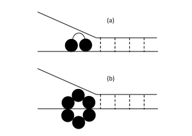
The concept of step size has been quite confusing in the helicase literature and sometimes gave rise to unnecessary controversies. A “mechanical step-size” should be defined as [1820] the average distance moved by the center of mass of the helicase per ATP molecule hydrolyzed by it. In contrast a “kinetic step-size” is defined [1820] is the average distance covered by the helicase in between two successive occurrences of the rate-limiting step of its mechano-chemical cycle. In general, these two step-sizes are not necessarily identical. Another quantitative characteristic of a helicase is its ATP-coupling stoichiometry [1820] which is the average number of ATP molecules hydrolyzed per base pair unwound; it differs from step-size when, for example, futile hydrolysis of ATP takes place.
One of the fundamental questions is the stepping pattern of a helicase on a single-stranded nucleic acid (ssNA)- is it analogous to hand-over-hand or inchworm pattern? Moreover, for this translocation on a ssNA, what is the mechanism of energy transduction- power stroke or Brownian ratchet? Furthermore, does it unzip the nucleic acid actively or passively? In the passive mode, it exploits (a) spontaneous opening of base pairs by thermal fluctuations, and (b) its own ability for directional translocation on ssNA to move forward, and stabilize the ssNA, before the base pair can close again. In contrast, in the active mode, it directly induces local destabilization of the dsNA instead of relying solely on thermal fluctuations for base-pair opening.
26.1 Non-hexameric helicases: monomeric and dimeric
A few helicases are monomeric. Dimeric helicases are more common. Two different types of ssNA translocation patterns have been postulated for different types of non-hexameric helicase motors- (i) stepping, and (ii) Brownian ratchet. In the stepping model, the helicase much have at least two NA-binding sites on it. In the case of monomeric helicases, usually these binding sites are located on two different domains whereas each of the two monomeric constituents of a dimeric helicase can have a NA-binding site on it. Inchworm is the most common stepping pattern although sometimes the experimental observations are also consistent with a “rolling” pattern which is the analog of the hand-over-hand stepping pattern of cytoskeletal motors.
The Brownian ratchet mechanism of non-hexameric helicase translocation on ssNA does not require more than one NA-binding site on the helicase. However, ATP-hydrolysis can cause a transition between two different conformational states in one of which the helicase has strong affinity for the NA whereas in the other it as weak affinity. Analog of the hand-over-hand mechanisms of the cytoskeletal motors is called the “rolling” model. However, most of the dimeric helicases are believed to follow the inchworm mechanism.
An oversimplified model for helicase motors was developed by Chen [1821]. A stochastic model for non-hexameric helicases was developed by Betterton and Jülicher [1822, 1823, 1824]. This model has been extended by Garai et al.[1825] to capture the effect of the ATPase activity of the helicase on its affinity for its nucleic acid track. HCV helicase NS3 is a representative member of the non-hexameric helicases that have been studied extensively [1826, 1827]. A limiting case of the model studied by Garai et al.[1825] corresponds to a Brownian ratchet mechanism for the NS3 helicase of HCV. Coarse-grained modeling of this helicase by elastic networks and NMA of the model has provided insight into its conformational kinetics in each cycle [1828, 1829].
26.2 Hexameric helicases
A large number of helicases are hexameric and have an approximate
ring-like architecture [1831, 1832, 1833, 1834, 1835].
For hexameric helicases, at least three
alternative mechanisms of enzymatic activities have been suggested;
these include, activities of all the ATP-binding domains in
(i) parallel, (ii) random, (iii) sequential manner.
(i) Parallel: In this mechanism all the subunits hydrolyze dTTP and
exert power stroke simultaneously.
(ii) Random: there are at least two possible different scenarios:
(a) random in time, where power stroke of each subunits starts and
finishes at random times independent of other units;
(b) random in space, where power strokes are sequential in time (i.e.,
each subunit can begin only after another finishes), but the order of
power strokes around the ring is random.
(iii) Sequential: there are at least two different sequences in which
the subunits can exert power stroke:
(a) paired sequential, i.e., sequentially around the ring, but with
diametrically opposite subunits in the same state;
(b) ordered sequential, i.e., sequential in the strict order 1,2,…6
around the ring.
Doering et al.[1833] developed a “flashing-field model” for DNA unwinding by hexameric ring-like helicases. This quantitative model is based on the following main assumption: ATP binding and hydrolysis induces conformational changes in the helicase that expose a pair of oppositely charged regions near the inner surface of the central channel of the ring. The negatively charged phosphates on the backbone of the DNA interact sequentially with this charge pair. The “flashing” charge pair gives a pulse of electrostatic push to the DNA before switching off in each cycle. Thus, in this model, the helicase is assumed to operate as a mechano-electrical transducer that transduces mechanical strains created by the conformational changes induced by ATP hydrolysis into an electrostatic force. It is this electrostatic force that, in turn, pushes charged DNA through the central channel of the helicase. It is not a Brownian ratchet; the Brownian force acts only as a “lubricant” reducing the stickiness caused by local minima in the free energy landscape.
In the mathematical formulation of the model, Doering et al. [1833] placed the coordinate system on the DNA so that the helicase motor executes a helical motion on this DNA track. Using a cylindrical coordinate system, the motion of the helicase is described by the two coordinates, namely, the azimuthal angle and the axial coordinate . The corresponding Langevin equations are [1833]
| (265) |
The configuration of dipoles switches from one configuration to another; in the -th configuration the full potential is given by [1833]
| (266) |
where is the total number of configurations. The potential has the form
| (267) |
with
| (268) |
where is the coordinate along the DNA charges, is the inverse screening length, and is the off-axis distance of the charges on the DNA backbone.
26.3 Section summary
In this section we have reviewed the few models of helicase motors that have been reported so far in the literature. The mechanisms of coordination of the multiple ATPase domains in both hexameric and non-hexameric helicases are not well understood at this stage. There is a need for distinct theoretical models based on different plausible mechanisms of coordination of the ATPase domains of a single helicase motor. The predicted collective behaviour of these competing models can be compared with experimental data to rule out some of the speculated mechanims.
27 Rotary motors I: ATP synthase (F0F1-motor) and similar motors
In section 16 we have discussed generic models of rotary motors to highlight the common features of their operational mechanism. Now, in this and the next sections, we review the kinetics of two most important rotary motors in living cells [1845, 1846, 1847], namely, ATP synthase and the bacterial flagellar motor, respectively, pointing out their main differences.
The models of specific rotary motors are usually based on the construction of a structural model of the stator and rotor at an appropriate level of details. For modeling its stochastic kinetics one assumes (i) the trajectories of the ions through the model structure, and (ii) the nature of the interactions among the (a) stator, (b) rotor, (c) the mobile ions, and (d) the hydrophobic environment of the membrane in which the motor is embedded. These dynamic interactions give rise to the coupling between ionic movements and the directed (on the average) rotation of the rotor. Significant progress have been made in understanding the mechanism of operation of these motors by a combination of structural studies and single-molecule experiments [186]. We have already seen that Na+ can substitute for H+ as the coupling ion in secondary transporters. H+ is not essential also for the operation of ATP synthases and in some ATP synthases Na+ is used instead of H+.
In this section we review the kinetics of ATP sythase (also called F-ATPase, for reasons explained in the next subsection) as well as those of two other similar rotary motors, namely V-ATPase and A-ATPase. (which we describe in detail in the corresponding subsections) [1847]. These rotary motors in living cells are wonderful achievements of nature’s evolutionary design. These can rotate at speeds exceeding even 100 revolutions per minute, generate torques as large as about 50 pN.nm and transduce energy at efficiencies that are vey close to . There are also some interesting architectural similarities between the ATP synthase and the TrwB DNA translocase.
27.1 Rotary motor F0F1-ATPase
ATP synthase is the smallest rotary motor and is embedded in membranes. In bacteria it is located on the cytoplasmic membrane whereas in eukaryotes it is embedded in the membrane of specialized organalles called mitochondria (in animal cells) and chloroplasts (in plant cells) [1848, 1849, 1850, 1851, 1852, 1853, 1854, 1855, 1856, 1857, 1858, 1859, 1861] (see appendix E for a brief introduction to these organelles and ref.[1862, 1863] for the history of the discovery of ATP synthase and its mechanism from the personal perspective of some of leading contributors).
Figure NOT displayed for copyright reasons.
The free energy input for ATP-synthase is IMF and the final output is freshly synthesized ATP. Each ATP synthase consists of two coupled parts which are called F0 and F1. ATP synthase is also referred to as F0F1-ATPase. Individually, both F0 and F1 are rotary motors. ATP synthase motor is reversible [1864, 1865] (see fig.52). In the ATP-synthesis mode, for F0 motor, an IMF across the membrane is the input and the rotation of F0, caused by the torque generated by the free energy transduction, is the corresponding mechanical output. Rotating F0, drives the shaft that, in turn, rotates F1 where ATP is synthesized from ADP and inorganic phosphate. In the reverse mode, free energy input from ATP hydrolysis is transduced by F1 to power the rotation of the shaft in the reverse direction thereby rotating F0 also in reverse while the latter operates effectively as a proton pump.
The F1 subunit has a threefold symmetry so that in a complete rotation by it synthesizes 3 molecules of ATP. However, the number of protons powering the corresponding rotation of the F0 subunit depends on the organism; for some organisms it is 10 whereas for some others it is 15 although even 12 and 13 are also quite common. Therefore, the ion-to-ATP ratio (the “stoichiometry”) can vary between 3.3 to 5. Since flow of protons across a PMF of would be utilized to synthesize a single molecule of ATP, one would expect . Perhaps, the organisms have optimized the “stoichiometry” and the IMF by adapting to the environment of their habitat [1866, 1867]. Therefore, understanding the operation of the ATP synthase motor requires addressing questions on the mechanisms of the rotary motors F0 and F1 separately and, then, their integration [1868].
The subunits of an ATP-synthase can also be clustered into two groups- those forming the parts of the “rotor” rotate with respect to a “stator” that consists of several other subunits. Interesting comparison of the rotation of F0 and F1, with the stepping of linear motors has been presented by Kinosita et al. [1869] and Junge [1870].
27.1.1 F0 motor: Brownian ratchet mechanism of energy transduction from PMF during ATP synthesis
The two main components of F0 motor are the stator and the cylindrical rotor which are separated by a narrow gap in between. Normally, the rotor consists of 12 identical segments each of which has a special negatively charged site on its surface that can be neutralized by adsorbing a single proton (protonation). Out of these twelve rotor subunits, two lie at the stator-rotor interface (see fig.53). There are two proton “half-channels” that are offset with respect to each other. Protons get access to one of the two rotor sites through the half channel that leads from the high-proton concentration side (acidic side) of the membrane to one of the two sites in front of the stator. Proton on the second site in front of stator can escape to the low-proton concentration site (basic side) of the membrane through the other half channel. This asymmetry of the two half-channels plays a crucial role in the rotational motion of the rotor (see figs.53 and 54). Moreover, there is a positively charged site midway between the two proton channels. As we discuss below, the Coulomb repulsion between this proton and those on the rotor sites enhances the efficiency of the rotary motor F0.
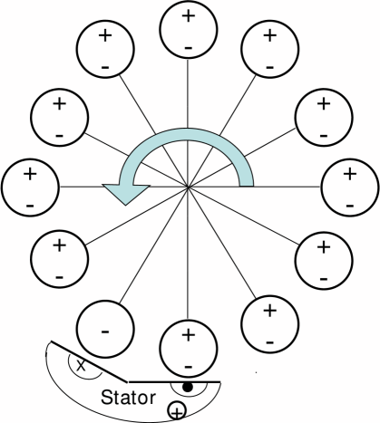
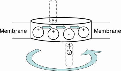
The operational mechanism of F0 motor was proposed in the mid-1990s by several groups (see, for example, [1871, 1872, 1873, 1874, 1875]). But, all these provided mostly qualitative pictures rather than quantitative predictions. To our knowledge, the first mathematical model of F0 motor was developed by Elston et al.[1876] (see also reviews in ref.[1877, 1878, 1879]). The original version of this model [1876] was formulated for PMF. Later similar treatments for SMF were also published [1880, 1881] although the details differ. The mechanical state of the F0 motor can be described by its angle of rotation around the central axis of the cylindrical rotor. The chemical state of the motor is denoted by the state of protonation of the two sites in front of the stator. The four possible chemical states are denoted by (both sites empty), (right site protonated), (fully, i.e., both sites protonated), and (left site protonated). Elston et al. [1876] assumed that direct hopping of protons from one site to another is not possible. Therefore, transitions between the states and involved at least 2 steps. A direct transition between and indicates a mechanical rotation rather than a chemical transition.
| (278) | |||
| (279) |
The Langevin equation describing the rotational motion is essentially a torque-balance equation:
| (280) |
where is the viscous drag coefficient and the different sources of torque shown on the right hand side, in general, depend on the chemical state . Alternatively, equations (279) and (280) can be combined into a single hybrid equation which is a combination of Fokker-Planck and master equations [1876].
The effect of the membrane potential, which was not incorporated in the kinetic equations by Elston et al.[1876], was taken into account in the corresponding equations for the Na+-ion-driven F0 motor formulated later by Dimroth et al.[1880]. In this equation ‘
| (281) |
labels the 16 distinct chemical states.
Most of the results for these models of F0 motor were obtained by solving the FP equations numerically. Bauer and Nadler [1882] developed a simpler model for the F0 motor that could be treated analytically. Instead of considering a pair of sites protected by the stator, this model focusses attention on a single site (more appropriately, a single “protomer”). The movement of a protomer by one protomer is described asa cyclic process. A cyclic spatial variable denotes its spatial location while the subscripts and indicate the states of its protonation (i.e., deprotonated or protonated). Let and be the probability densities for a protomer unit of the F0 motor to be located at and in the deprotonated and protonated states, respectively, at time . The FP equations governing the time evolution of the system are [1882]
| (282) | |||
| (283) |
where accounts for the “chemical” transitions
| (284) |
In general, the diffusion constants depend not only on , but also on the “chemical” state (i.e., the state of protonation). The force and account for the interactions of the rotor with its surroundings; it can be derived from an appropriate local potential.
A model of F0-type motors was developed by Smirnov et al.[1883] using the theoretical formalisms that are usefully applied in condensed matter physics. The Coulomb interaction between the stator and rotor charges was shown to be dominant contributor to the torque that rotates the F0 motor.
All the models of F0 discussed so far in this review are essentially one-dimensional in the sense that the only mechanical movement allowed is the pure rotation (described by ) of the rotor unit that is effectively treated as a rigid body. A more detailed description of the possible mechanical movements of the stator-rotor combination emerged from MD simulation of an atomistic structural model [1884] of the system up to nanoseconds. Incorporating several of such different degrees of freedom in a coarse-grained model, a stochastic kinetic model of F0 was developed by Aksimentiev et al. [1860]. Although this kinetic model also assumes a Brownian ratchet mechanism, this extended version is often referred to as a “protein-roller bearing mechanism” [1861]. Its numerical simulation over millisecond time scales provided a deeper insight into the underlying mechano-chemistry than that obtained from the older model of Elston et al.[1876].
27.1.2 F1 motor: power stroke mechanism in reverse mode powered by ATP hydrolysis
The F1 motor consists of a hexameric complex that looks somewhat like a skinned orange and is composed of alternating and subunits; this structural organization is often denoted symbolically as . The ATP-binding site is located on the subunits in the cleft between and . ATP hydrolysis drives a central “shaft”, called -subunit, by executing a power stroke.
Binding-change, cooperativity and rotational catalysis
The three main ingredients in the mechanism of operation of F1 are
as follows [1890, 1891, 1892, 1893, 1894, 1895]:
(i) binding-change: the input energy is used not to form the ATP
molecule, but to drive the release of an already formed molecule of ATP
from the binding site.
(ii) catalytic cooperativity: each of the three catalytic sites of
F1 goes through three kinetic states in a cycle, but the cycles of
the three are staggered. A catalytic site can be in one of the three states
labelled by E (empty), T (tightly bound to substrate/product) and
L (loosely bound to substrate/product). The three catalytic sites in F1
operate cooperatively in such a way that ATP cannot be released from
one site unless ADP and Pi bind to another site while the third site
is empty.
(iii) rotational catalysis [1896, 1897]: the ion transport
in the F0 subunit is coupled to the ATP synthesis in the F1 subunit
through rotation of the hexamer.
Binding-zipper model
In the binding-zipper model [1878], in the reverse mode of operation of the F0F1 motor, ATP binding to a catalytic site on F1 takes place in a progressive manner by the sequential formation of bonds between the ATP molecule and the catalytic site. Conversely, in the ATP synthesizing mode, the binds bonds holding the freshly synthesized ATP molecule are broken (unzipped) sequentially. Thus, the binding-zipper model has been interpreted as an extension of the induced fit model of enzyme specificity (which we discussed in section 6); the single-step substrate-binding is replaced in this extended model by a multi-step binding process where bonds are formed between the substrate and the catalytic site sequentially [1878]. Supporting evidences for the binding-zipper model have emerged from computer simulations of the unbinding and binding of ATP to and from the F1 motor, respectively [1898, 1899].
Figure NOT displayed for copyright reasons.
The model for the ATP synthase operating in the “ATP hydrolysis mode”, i.e., in the mode in which F1 hydrolyzes ATP to function as a chemically-powered rotary motor, has been developed by Oster and coworkers [1886, 1888]. The corresponding model for the ATP synthase running in the “ATP synthesis mode”, also developed by Oster’s group [1887], utilizes essentially the same underlying structural features of the motor. In the ATP synthesis mode, rotary motion of the eccentric -shaft is converted into the “hinge-bending” motion of the -subunits by a mechanism that is analogous to the vertical movement of automobile jack by turning the crank (see fig.55). Conversely, in the ATP hydrolysis mode the hinge-bending motion of the -subunits are converted into the rotation of the -shaft [1889]. The physical reasons for the surprisingly high mechanical efficiency of the F1-ATPase have been explained by Oster and Wang in terms of underlying molecular mechanisms [1885].
Gaspard and Gerritsma [1900] developed a mechano-chemical kinetic model. In this model the 6 chemical states are assumed to be adequate while for the mechanical state only a single angular variable is introduced.The dynamics of the system is formulated in terms of a hybrid set of equation that describes the changes in by the FP-like terms and changes in the chemical states by master-equation-like terms for discrete jump processes. The results are consistent with a tight mechano-chemical coupling for the F1 motor. In a subsequent work, Gerritsma and Gaspard [1901] replaced the continuous angle by a discrete 2-state model whose kinetics is governed by a set of master equations. Exact analytical expressions could be derived for the average angular speed of the -shaft and to show that it obeys a Michaelis-Menten-like equation with respect to the ATP concentration [1901]. For sufficiently low external torque, the results are consistent with a tight mechano-chemical coupling of the F1 motor.
27.1.3 F0-F1 coupling
In the two preceding subsubsections we have separately discussed the kinetics of the operations of the individual F0 and F1 subunits of the F0F1- ATPase. Now we briefly review the theoretical models of coupling the two subunits for the overall operation of the F0F1 motor.
For a long time, elastic power-transmission has been a serious candidate for explaining the mechanism of coupling between F0 and F1 [1902]. Cherepanov et al.[1903] developed a stochastic kinetic model of ATP synthase assuming an elastic coupling between F0 and F1. The 4 kinetic states are essentially same as the states E, L, F and R in the model developed by Elston et al.[1876]. Suppose the elastic coupler is in a relaxed at an instant of time when the angular position of the rotor is . In the kinetic scheme formulated by Cherepanov et al.[1903], the four transition increase the strain in the elastic coupler in a stepwise manner. Then the release of the elastic strain triggers the release of the ATP molecule synthesized in the F1 subunit without causing any angular displacement of the rotor during this release of ATP. Using this kinetic model for the analysis of the channel conductance data it has been claimed that the F0 is not voltage-gated [1904].
A mesoscopic model of elastic coupling, developed by Czub et al. [1905] treats the F0-F1 coupling device as eight segments that are stacked layers each of which is harmonically coupled to its neighboring segments. This model may be viewed as an extension of the model developed earlier by Cherepanov et al. [1903].
27.2 Rotary motors similar to F0F1-ATPase
In this subsection we briefly describe two rotary motors that share many of the characteristic features of the structure and dynamics of F0F1-ATPase.
27.2.1 Rotary motor V0V1-ATPase: a “gear” mechanism?
Vacuolar ATPases were initially identified in plant and fungal vacuoles and hence the name. Later these were found also in plasma membrane and organelle membranes of mammalian cells and plants. Therefore, it is more appropriate to link the letter “V” in V-ATPase with “various” (various membranes) rather than “vacuoles”. V-ATPases operate in-vivo as ATP-dependent proton pumps that regulate the pH (acidify) intracellular compartments in eukaryotic cells [1906, 1907, 1908, 1909, 1910, 1911, 1912, 1913, 1914, 1915, 1916, 1917, 1918, 1919] (for a historical account, from the personal perspective of one of the leading contributors, see ref.[1920]).
Just like F0F1 motors, V-ATPases also consists of V0 and V1 domains [1921]. The V0 domain is located on the cytoplasmic side of the membrane whereas V0 is embedded in the membrane. V1 hydrolyzes ATP to drive the proton pump V0 whereby protons are translocated from the cytoplasm to the other side of the membrane. Unlike F0F1, V0V1 does not synthesize ATP from ADP. One key structural difference, which has functional implications, is that F0 normally has 12 proton carriers whereas V0 has only 6.
A mechano-chemical model of the V0ion pump was developed by Grabe et al.[1922] along the same line as followed by Elston et al. [1876] for formulating their model for the F0 ion pump. However, unlike the two-channel (more appropriately, two half-channels) model of the F0 ion pump, both two-channel and one-channel models are possible for V0 [1922]. The two-channel model of V0 is very similar to the two-channel model of F0. In contrast, in the one-channel model the proton-binding sites on the rotor are assumed to be just outside the level of the membrane and in equilibrium with the cytoplasm. Therefore, no channel is required for protonation of the proton-binding sites. Rotation bring a protonated site to the entrance to the channel where the stator charge forces its release from the binding site and passage through the channel to the other side of the membrane. The binding site that gets unprotonated in this process can continue its further rotation provided a narrow polar strip creates a corridor for it to make an exit to the cytoplasm where it again gets protonated.
An interesting prediction of the model of Grabe et al.[1922, 1923] is the possibility of a “gear” mechanism. Suppose three of the six rotor sites of the V0 pump withdraw from proton pumping. Then, the pumping rate would be slower but would be able to account for a much higher PMF. This is the analog of a gear changing that would generate larger force but smaller speed. Grabe and Oster [1922] have developed a detailed quantitative kinetic theory of the regulation of organelle acidity incorporating the pumping of protons by V-ATPase.
27.2.2 Rotary motor A0A1-ATPase
A-ATPases can function as either ATP synthase mode or in the ion-pump mode. Detailed comparison of the structures and functions of A-ATPases and V-ATPases have been reported [1924, 1925, 1926]. The number of ion-binding sites on A0 can vary from 6 to 13 giving rise wide variability of the stoichiometry [1927].
The mechanisms of torque generation by the ATP synthase (or, F0F1-ATPase) in both the ATP-synthesizing and ATP-hydrolyzing modes have been investigated in great detail. The mechanism of the coupling of the two components, namely F0 and F1 is also fairly well understood.
28 Rotary motors II: Flagellar motor of bacteria
The flagellum is one of the most important prokaryotic motility structures [1928, 1929]. The diameter of the bacterial flagellar motor (BFM) is approximately 50 nm and its angular speed can be as high as rpm. Any satisfactory model of BFM [1930, 1931, 1932, 1933, 1934, 1935] has to be reversible because bacteria are known to switch the motor from CW to cCW and vice-versa.
A bacterial flagellum has three major parts: a rigid helical filament, a flexible hook and a basal body. The hook joins the filament with the basal body. The motor of the bacterial flagellum is located in the basal body which consists of a set of concentric rings mounted on a rod that passes through the central axis. The rings have been named according to their layer of the cell envelope in which they are located: L-ring (named after lipopolysaccharide), P-ring (named after peptidoglycan), S-ring, M-ring, etc. For our purpose here, we’ll refer to these rings collectively as simply the “ring”. Each BFM has several independent stators. The structure of the bacterial flagellum has been analyzed from an evolutionary perspective, i.e., how the flagellar structure in the living bacteria today might have resulted in the course of Darwinian evolution from its more primitive ancestors [1936].
The wealth of experimental data collected over the decades have imposed constraints on models of the BFM [1937]. Until about 40 years ago, it was commonly believed that each flagellum propagates a helical wave. But, Berg and Anderson [1938] emphatically argued that the experimental evidences indicate rotation of each of the flagella. Taking hint from the existing experimental results, they assumed that the flagellum is rigidly coupled to the “M-ring” which is free to rotate within the cytoplasmic membrane. However, they also imagined that the periphery of the M-ring would be linked to the cell wall by actomyosin-like “cross-bridges”, whose real identity was unknown, that would exert the torque to rotate the M-ring. Thus, this scenario is based on a Brownian ratchet mechanism of free energy transduction. This idea was expanded and quantified by Khan and Berg [1939, 1940]. Several variants of this model as well as many other models [1941, 1942, 1943, 1944, 1945, 1946, 1947, 1948] developed during the first twenty years of activity following Berg and Anderson’s work [1938] have been reviewed [1940, 1949, 1950, 1930, 1931, 1933, 1934, 1935]
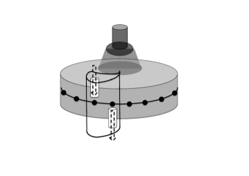
In the “turnstile” model [1942, 1845, 1933], (see fig.56) ions entering the bacterial cell from its external surroundings take a ride on the rotor. The rotor itself moves either because of electrostatic interactions among various charges on the rotor and stator or because of its own rotational Brownian motion. Each of the hitch-hiking ions disembark from the rotor after getting transported up to a certain distance by the rotor. Once the ion leaves, the rotor remains “locked” in its current position thereby completing one step of its rotational movement and waits for the arrival of the next ion. The key features of this mechanism are very similar to those of the F0 motor that we discussed earlier in this section.
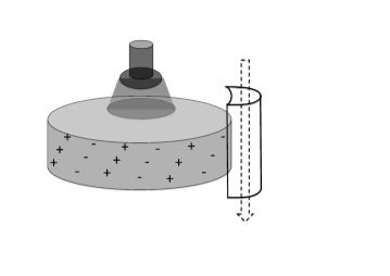
Among the earliest models of BFM that remain relevant even today, to my knowledge, the first one was proposed by Läuger [1943] and is based on the so-called “turbine” mechanism (see fig.57). In this model both the rotor and stator are assumed to be decorated with rows of chemical groups, called “half-sites”. The special feature of these sites is that that individually each is incapable of binding to a proton, but become competent to bind a proton when paired up with another “half-site”. The rows of the half-sites on the rotor are tilted with respect to the vertical row of half-sites on the stator. Therefore, at any arbitrary instant of time, the row on a given stator intersects a row on the rotor at a single point which forms the only proton-binding site at that instant of time. With the turning of the rotor, the point of intersection of the stator row and rotor row move across the vertical surface of the rotor. Therefore, if protons are constrained to move vertically hopping from one binding site to the next, along their concentration gradient, vertical proton flow would drive the rotation of the rotor in the horizontal plane. Moreover, a conformational change that reverses the title angle of the rows of half-sites on the rotor would account for the switching of the direction of rotation.
The original version [1943] of the “turbine” model of BFM was improved in its subsequent amendments [1944, 1945]. The essential feature of the “turbine” models is the rows charges that are tilted with respect to the ion channels in the stator. The tilted rows on the rotor need not be “half-sites”, as assumed originally by Läuger [1943]. An alternative possibility of alternating rows of positive and negative charges has also been explored [1951, 1952]. In these “ion turbine” models, the positively charged ion moves exclusively along an ion channel in the stator and never moves onto the rotor. As the positively charged ion moves along the channel, it tends to keep a row of negative charges on the rotor close to it. Consequently, the rotor rotates as the positively charged ion transits through the channel. This situation is analogous to hydro-electric turbines; the positively charged translocating ions are the analogs of water while the tilted rows of charges are the analogs of the turbine blades. Just as the water flowing through the turbine exerts torque on the rotor unit, the translocating ion in the BFM exerts torque on the corresponding rotor [1951]. Because of this analogy, this class of models are referred to as “turbine” [1951, 1952]. The CW-cCW switching can be explained by the change in the proton affinity of the proton-binding sites of the channel. When the proton-affinity is high the ionic current is carried by protons (+ve charge) into the cell whereas in the opposite case of low proton-affinity the effective ionic current is that of -vely charged “holes” flowing outward from the cell. The flipping of the sign of the effective carriers of ionic current leads to the CW-cCW switching.
Let us assume that there are just 2 sites available in each proton channel for their protonation. The 4 possible states of the channel are then [1952] denoted by the symbols E (both sites empty), T (top site occupied by a proton), B (bottom site occupied by a proton), and F (both sites full). The probabilities for the occurrence of these four states are the components of the column vector where denotes the angular position of the of the rotor at time . The kinetic equation for can be expressed as [1952]
| (285) |
where is the Fokker-Planck operator describing the mechanical rotation whereas is the master operator that accounts for the changes in the occupation of channel sites by protons. The operator incorporates not only rotational diffusion term but also rotational drift caused by electrostatic potentials where the angular profile of the potential, in general, depends on the state of occupation of the designated sites by the protons [1952]. In this model the protons modulate the interactions of the negatively charged proton-binding sites with rotor charges by screening (or neutralizing) these negative charges. In the subsequent work of Walz and Caplan [1953] the protons are directly responsible for the torque generation.
Kojima and Blair [1954] proposed a power stroke mechanism in which a conformational change of the stator, caused by the inflow of a proton (or sodium ion) into the embedded channel, drives the rotation of the rotor. Schmitt [1955] proposed a different mechanism of electrostatic transmission of force from the stator to the rotor. In this model the passage of proton or sodium ion induces a reversible rotation of the stator that, in turn, rotates the rotor because of their electrostatic interaction at the stator-rotor interface. These ideas were extended even further, with minimum number of assumptions regarding the generic principles, by Xing et al. [1956] and Bai et al.[1957, 1958]. It was pointed out that there are two time scales in the system, namely, (a) the time scale of ion hopping on and off (the intrinsic dynamics), and (b) the time scale of relaxation of the load spring (an extrinsic dynamics). This time scale separation gives rise to a plateau in the force-velocity plot [1956]. The fact that the stators move approximately independent of each other allows a mean-field type approximation. Exploiting this simplification, Bai et al.[1958] have developed a unified theory that explains the coupling between the torque generation and the dynamics of switching between CW and CCW rotation.
28.1 Summary of the sections on rotary motors
In this section and the preceeding section we have reviewed the models of two major classes of rotary molecular motors. Let us now draw analogy between the swimming of a single bacterium by multiple flagella, each of which is driven by a distinct rotary motor, and the transport of a single vesicular cargo by multiple cytoskeletal motors. In the latter case, as we have discussed in the subsection 17.5, significant progress has been made in recent years on the multi-motor cooperativity. However, in contrast to cytoskeletal motors, each BFM is a reversible rotary motor. Therefore, a kinetic model of the collective operation of the BFMs of a single bacterium should not only explain the mechanism of their cooperative rotation, but also their coordinated switching.
29 Some other motors
Myosin-I: membrane-cytoskeleton active crosslinker
Among the unconventional myosins, myosin-V and myosin-VI have been discussed in detail in section 17.1. Here we briefly describe the special features of the members of another family of unconventional myosins, namely myosin-I.
Myosin-I can bind simultaneously to actin filaments and cell membranes thereby crosslinking the two. However, unlike other passive crosslining proteins, myosin-I crosslinks actively in the sense that it can bend, deform and move membrane by coupling these operations with ATP hydrolysis that it catalyzes. These operations of myosin-I are part of many biological functions that include, for example, exocytosis, endocytosis, vesicle shedding, blebbing and gating of ion channels [1959]. All these biological processes have been modelled theoretically. But, to my knowledge, the mechanism of force generation by a single myosin-I motor in terms of its structure and mechano-chemical kinetics remains a challenging open problem.
Chromatin remodellers and unwrapping of nucleic acids
If nucleosomes were static, segments of DNA buried in nucleosomes would not be accessible for various functions involving the corresponding genes. In order to get access to the relevant segments of DNA for various processes in DNA metabolism, eukaryotic cells use ATP-dependent chromatin-remodeling enzymes (CRE) which alter the structure and/or position of the nucleosomes [182, 1960, 1961, 1962, 1963, 1964, 1965, 1966, 1967]. In principle, there are at least four different ways in which a CRE can affect the nucleosomes [1967]: (i) sliding the histone octamer, i.e., repositioning of the entire histone spool, on the dsDNA; (ii) exchange of one or more of the histone subunits of the spool with those in the surrounding solution (also called replacement of histones) (iii) removal of one or more of the histone subunits of the spool, leaving the remaining subunits intact, and (iv) complete ejection of the whole histone octamer without replacement.
Spontaneous thermal fluctuations can cause a transient unwrapping and rewrapping of the nucleosomal DNA from one end of the nucleosome spool. On the nucleosomal DNA, the farther is a site from the entry and exit points, the longer one has to wait to access it by the rarer spontaneous fluctuation of sufficiently large size [1968, 1969, 1970, 1971].
Can a nucleosome slide spontaneously by thermal fluctuations thereby exposing the nucleosomal DNA? If the DNA were to move unidirectionally along its own superhelical contour on the surface of the histone, at every step it would have to first transiently detach simultaneously from all the binding sites and then reattach at the same sites after its contour gets shifted by bp (or multiples of bp). But, the energy cost of the simultaneous detachment of the DNA from all the binding sites is prohibitively large [1972, 1973, 1974].
But, why can’t the cylindrical spool simply roll on the wrapped nucleosomal DNA thereby repositioning itself? If the nucleosome rolls by detaching DNA from one end of the spool, cannot it compensate this loss of binding energy by simultaneous attachment with a binding at the other end? This rolling mechanism would successfully lead to spontaneous sliding of the nucleosome only if the histone spool were infinite with an infinite sequence of binding sites for DNA on its surface; however, on a finite-size histone spool this would not be feasible [1972].
An alternative possibility is to form a flap that can diffuse. In the process of normal “breathing”, most often the spontaneously unwrapped flap rewraps exactly to its original position on the histone surface. However, if the rewrapping of a unwrapped flap takes place at a slightly displaced location on the histone spool a small bulge (or loop) of DNA forms on the surface of the histones. Since the successive binding sites are separated by bp, the length of the loop is quantized in the multiples of bp [1975]. Such a spontaneously created DNA loop, can diffuse in an unbiased manner on the surface of the histone spool. In the beginning of each step DNA from one end of the loop detaches from the histone spool, but the consequent energy loss is made up by the attachment of DNA at the other end of the loop to the histone spool before the step is completed. Consequently, by this diffusive dynamics, the DNA loop can traverse the entire length of the binding sites on the histone spool of a nucleosome which will manifest as sliding of the nucleosome by a length that is exactly equal to the length of DNA in the loop. The diffusing DNA bulge can be formed by a “twist”, rather than bending, of DNA [1976, 1977, 1978]. Spontaneous sliding of a nucleosome, however, is too slow to support intranuclear processes which need access to nucleosomal DNA. That is why ATP-dependent CRE is needed for active remodeling of the nucleosome.
Various aspects of chromatin dynamics has received some attention of theoretical modelers, including physicists, over the last few years [1979, 1975, 1973, 1974, 1980, 1981, 1972, 1982, 1983, 1984, 1985, 1986, 1987, 1988, 1989].
FtsK and SpoIIIE: Chromosome segregation motors in E-coli and Bacillus subtilis
So far there are no convincing direct evidence for the existence of any mitotic spindle-like machinery in bacteria for post-replication segregation of chromosomes before cell division. However, there are more primitive motors which carry out chromosome segregation in bacteria. For example, in E-coli FtsK segregate chromosome in an ATP-dependent manner by translocates dsDNA during cell division [1990, 1991, 1992, 1993, 1994, 1995, 1996].
Normally Bacillus subtilis, a rod shaped bacterium, divides to two similar daughter cells. However, under some special circumstances, which leads to spore formation, a Bacillus subtilis divides asymmetrically into a small prespore and a larger mother cell. The translocation of the chromosome into the small prespore compartment is carried out by the motor protein SpoIIIE.
Most of the fundamental questions on the operational mechanism of FtsK and SpoIIIE are similar to those generic ones for helicases and translocases (including packaging motors for viral capsids). For example, how does SpoIIIE, which anchors itself at the septum between the two compartments, translocate the DNA in the desired direction, namely, from the larger to the smaller compartment?
G-proteins
G-proteins, which are believed to be the common evolutionary ancestors of myosins and kinesins [588], also generate forces by hydrolyzing GTP. The force thus generated are comparable to that generated by myosin and kinesin both of which are powered by ATP hydrolysis [1997].
Topoisomerases and untangling of DNA
As we mentioned in subsection 4.1.2, topoisomerases can untangle DNA by passing one DNA through a transient cut in another. Topoisomerases are broadly divided into two classes, namely type I and type II, which cleave one or two strands of DNA, respectively [1998, 1999, 2000, 2001, 2002, 2003, 2004, 185]. In principle, mere strand pasage reaction catalyzed by a topoisomerase does not require input energy- the chemical energy of the cleaved phosphodiester bond (or bonds, in case of type-II topoiomerase) is stored within the DNA-enzyme complex and, therefore, can be utilized for the restoration of the bond(s) after the strand passage. Indeed, type-I topoisomerases perform the task of strand passage without the consumption of external energy. Then, why do type-II topoisomerases hydrolyze ATP for the same task?
Classic experiment of Rybenkov et al.[2005] established that the type-II topoisomerase are capable of suppresing the probability of self-entanglement (i.e., knots) and mutual entanglements (i.e., links) far below the levels expected from equilibrium statitical mechanics. In other words, type-II topoisomerases not marely catalyze the strand pasage reaction, but also control the overall entanglement of the DNA molecule. In its latter role, it essentially acts as a Maxwell’s demon [2006, 2007] and does not violate the second law of thermodynamics becaue of the consumption of input energy supplied by ATP hydrolysis. The lower-than-equilibrium entanglement achieved by the type-II topoisomerases has been explained by a kinetic proofreading mechanim [2008] that, in spirit, is similar to the kinetic proofreading mechanism for lower-than-equilibrium error committed by a ribosome during translation.
For many years, it was not clear how a small machine like a topoisomerase can sense the DNA topology, which is a global property, through local DNA-protein interaction. In recent years, few alternative possible scenario have been proposed to explain this phenomenon [2009]; however, a detailed discussion of these models is beyond the scope of this review.
Chaperones and folding of proteins
Protein folding in-vivo is most often assisted by a group of molecular machines called chaperones [2010, 2011, 2012]. Members of many chaperone families are also known as heat shock proteins (HSP) and these families are classified according to their molecular weights, e.g., HSP60, HP70, HSP90, etc.[2013, 2014]. The operations of these machines are fuelled by ATP. Among the chaperones, the chaperonin proteins [2015, 2016, 2017] (GroEL in bacteria) have been characterized, both structurally and functionally, in great detail [2018, 2019, 2020]. The heptameric ring-like structure of GroEL resembles a cage where a lid is formed by GroES. Encapulation of a protein within the cage protects it against aggregation or misfolding. ATP binding and hydrolysis modulates the affinities of the GroES caps for the GroEL ring thereby regulating the release of protein (partially-) folded inside the cage. The concept of allosterism, that we explained in section 6.3.4, plays an important role in the kinetics of GroEL-GroES machinery. The positive cooperativity arising from the intra-ring interactions and the negative cooperativity caused by inter-ring interactions have been elucidated by molecular dynamic simulation [2021]. Tehver and Thirumalai [2022] developed a kinetic model that couples the allosteric transitions of the GroEL with the distinct stages of folding (or misfolding) of the protein substrate. The efficiency of the folding machinery is found to depend on the chaperonin concentration and the rate of binding of the protein substrate [2022].
Synthetic molecular motors: biomimetics and nano-technology
Initially, technology was synonymous with macro-technology. The first tools applied by primitive humans were, perhaps, wooden sticks and stone blades. Later, as early civilizations started using levers, pulleys and wheels for erecting enormous structures like pyramids. Until nineteenth century, watch makers were, perhaps, the only people working with small machines. Using magnifying glasses, they worked with machines as small as . Micro-technology, dealing with machines at the length scale of micrometers, was driven, in the second half of the twentieth century, largely by the computer miniaturization.
In 1959, Richard Feynman delivered a talk [2033] at a meeting of the American Physical Society. In this talk, entitled “There’s Plenty of Room at the Bottom”, Feynman drew attention of the scientific community to the unlimited possibilities of manipulating and controlling things on the scale of nano-meters. This famous talk is now regarded by the majority of physicists as the defining moment of nano-technology [2034]. In the same talk, in his characteristic style, Feynman noted that ”many of the cells are very tiny, but they are very active, they manufacture various substances, they walk around, they wiggle, and they do all kinds of wonderful things- all on a very small scale”.
From the perspective of applied research, the natural molecular machines opened up a new frontier of nano-technology [2035, 2036, 2037, 2038, 2039, 2040, 2041, 2042]. Even nano-robotics may no longer be a distant dream [2043, 2044]. A conventional 2-headed kinesin has strong resemblance, at least at a superficial level, with two-legged mobile robots (see ref.[2045] for a historical account of the development of legged robots, particularly the “bipeds”). The miniaturization of components for the fabrication of useful devices, which are essential for modern technology, is currently being pursued by engineers following mostly a top-down (from larger to smaller) approach. On the other hand, an alternative approach, pursued mostly by chemists, is a bottom-up (from smaller to larger) approach. The bottom-up approach is also likely to enrich synthetic biology [2046, 2047, 2048, 2049, 2050, 2051, 2052, 2053]. The term biomimetics has already become a popular buzzword [2039, 2040]; this field deals with the design of artificial systems utilizing the principles of natural biological systems. We can benefit from Nature’s billion year experience in nano-technology.
Importance of molecular motors in biomedical research- control and cure of disease
Just as occasional disruption of work in any department of a factory can bring entire operation factory to a standstill, defective molecular machines can cause diseases. Moreover, viruses are known to hijack the motors to travel from the cell periphery to the cell nucleus. If we understand how molecular machines work, we might be able to devise ways to selectively either arrest those sub-cellular processes that cause diseases like cancer or slow down metabolism of invading organisms. The molecular motor transport system can be utilized even for targeted drug delivery where molecular motors can be used as vehicles for the drug. Thus, fundamental understanding of the mechanism of biomolecular machines will help us to fix them when they malfunction and, perhaps, to manipulate them to improve human health and fitness.
30 Summary and outlook
In this article we have critically reviewed the stochastic kinetics
of molecular motors and that of the processes that they drive.
In part I, we have considered the fundamental principles, some essential
background concepts and generic models for several different types of
motors. Some of the common “chemical” proceses involved in their operation
are listed below:
(i) chemical reactions are catalyzed either by the motor itself or by
an accessory device;
(ii) The motor forms non-covalent bonds with substrates and other
ligands;
(iii) many conformations of the motor are possible and the motor
fluctuates between these conformations because the strengths of the
non-covalent bonds are comparable to the thermal energy ;
(iv) binding or unbinding of a ligand can alter the relative stability
of conformations thereby inducing transition from one to another.
Moreover, there are further formal similarities between the “mechanical”
stepping of a single motor and chemical reaction catalyzed by a
single enzyme molecule. Therefore, several aspects of the kinetics of
chemical reactions, particularly those catalyzed by enzymes, have been
discussed in significant detail in part I of this review. The strategies
of modeling stochastic mechano-chemical kinetics at different levels of
spatio-temporal resolution have also been explained before reviewing the
generic models.
In part II we have presented applications of these basic concepts and techniques of chemical physics as well as those of nonequilibrium statistical mechanics to study the stochastic kinetics of specific molecular motors using theoretical models. Some of the key structural details or important features of the kinetics of the motors, which were ignored in part I in the context of generic models, have been incorporated in the specific models of these motors in part II of this review. All the motor-driven movements reviewed here can be classified into four categories [12]: (i) rotation about an axis, (ii) translation along an axis, (iii) translation perpendicular to an axis, and (iv) lateral separation of two axes.
While summarizing each section, we have already listed some open questions in the context of specific motors. Next I list a few general open questions that can be raised for all the motors. Barring the exception of great visionaries, for anyone it is risky to speculate on the future directions of research on molecular motors. Neverthless, I point out some limitations of the current models so that the future course of action for theorists can be anticipated.
The atomistic structure of many motors are not known at present at sufficiently high-resolution (resolution of a few angtroms). Only when such high-resolution structures become available, fully atomistic in-silico modeling of the motor would be possible. However, even when such detailed structures are available, only coarse-grained models may be useful if the direct MD simulation of the atomistic models over the relevant time scales cannot be performed with the computational resources available.
For modeling at the coarser Brownian level, based on Langevin or Fokker-Planck equations, the potential landscape is needed. However, for most of the motors, these potential landscapes are postulated, rather than derived from more microscopic considerations. For example, there are compelling evidences that electrostatic interactions play important roles in the operation of the individual members of many families of molecular motors. However, so far very little effort has been made to derive the effective interactions (and potential landscapes) from more microscopic considerations where the electric charges and their coulomb interactions would be treated explicitly.
For solving the forward problem with process modeling, we expect significant progress over the next decade in two opposite directions: (a) in-silico modeling of single individual motors with ever increasing structural and dynamical details of its coordinating parts in an aqueous medium; (b) integration of nano-motors and motor-assemblies into a micro-factory- the living cell.
Finally, let me emphasize the need of statistical inference drawn from analysis of empirical data for reverse-engineering of molecular motors. In a rare example of model selection for a specific molecular motor, Bronson et al. [2286] extracted the best model by optimizing the maximum evidence, rather than maximum likelihood, that treats, for example, the number of discrete states of the system as a variational parameter. This is a step in the right direction. However, I am not aware of any work that ranks alternative models of any molecular motor according to relative scores computed on the basis of the principle of strong inference [86, 84].
The picture of the motor-driven intracellular processes in a living cell can be dramatized as follows [2287]: the cell is like an under water “metro city” which is, however, only about m long in each direction! In this city, there are “highways” and “railroad” tracks on which motorized “vehicles” transport cargo to various destinations. However, the highways and railroads are very dynamic- these are constructed when needed and often dismantled when not in use. It has a library for an efficienct storage of the chemically encoded blueprint of the construction and maintenance of the city. It has a system of machinery that provides rapid access to specific regions of this packaged blueprint. It has specialized machines that, utilizing the chemically encoded template stored in this library, synthesize materials that, then, form the components of various machine tools in this city. It has special “waste-disposal plants” which degrade waste into products that are recycled as raw materials for fresh synthesis. This eco-friendly city re-charges spent “chemical fuel” in uniquely designed “power plants”. This city also uses a few “alternative energy” sources, including “electrical” energy, directly in some operations.
A complete understanding of the running of this fully automated “under water metro city” in terms of the coordinated operation of the machineries would be the ultimate aim of scientific investigation on intracellular molecular motors. However, “such triumphant victories come very rarely, and they are separated by the slow, plodding attack on a wide front” [2288].
Appendix A Eukaryotic and prokaryotic cells: differences in the internal organization of the micro-factories
From the evolutionary point of view, cells have been, traditionally, divided into two categories, viz., prokaryotes and eukaryotes. Most of the common bacteria like, for example, Escherichia Coli (E-coli) and Salmonella, are prokaryotes. Animals, plants and fungi are collectively called eukaryotes. Major difference between prokaryotic and eukaryotic cells lies in their internal architectures; the main distinct feature of eukaryotic cells is the cell nucleus where the genetic materials are stored. The prokaryotes are mainly uni-cellular organisms. The eukaryotes which emerged first through Darwinian evolution of prokaryotes were also uni-cellular; multi-cellular eukaryotes appeared much later. The plausible evolutionary routes leading to the birth of the first eukaryotic cell from its prokaryotic ancestor(s) and its subsequent evolution is an active area of scientific exploration [2054, 2055, 2056],
Moreover, the traditional division into prokaryotes and eukaryotes has been questioned and an alternative three-domain system, that classifies organisms into bacteria, archaea and eukaryota, has been proposed [2084, 2085, 2086]. We’ll not get involved in the debate on the scheme for classification of organisms; for the purpose of this review, which is addressed mainly to physicists, we’ll use both the schemes hoping that the context will make the usage unambiguous.
Some of the molecular machines found in eukaryotes have been discovered also in the other domains in the kingdom of life. But, some other machines seem to be present only in eukaryotes. So far as the archaea are concerned, it is interesting to compare their machinery with those of bacteria and eukaryota. We’ll consider concrete examples in the appropriate contexts.
A.1 Model eukaryotes and prokaryotes
In biology, often the simplest among a family of objects is called a model system for the purpose of experimental investigations [2103]. A short list of the model systems commonly used in molecular cell biology, particularly those found useful for studying functions of molecular machines, is now provided.
The most popular model animals for biological studies are as follows: (i) the fruit fly Drosophila melanogaster, a model insect, (ii) Caenorhabditis elegans (C-elegans), a transparent worm, (iii) the zebra fish danio rerio, a model vertebrate; (iv) the mouse, however, is more important for practical use of cell biology in medical sciences.
Arabidopsis thaliana is the most popular model plant while Chlamydomonas reinhardtii is a model of green algae. Saccharomyces cerevisiae (Baker’s yeast) and Schizosaccharomyces pombe (Fission yeast) are most widely used models for fungi. However, for studying filamentous fungi, Neospora crassa is used most often as a model system.
Bacteria are divided into two separate groups on the basis of their response to a staining test invented by Hans Christian Gram. Those which respond positively are called Gram-positive bacteria whereas those whose response is negative are called Gram-negative. One of the main differences between these two groups of bacteria is the nature of the cell wall which we’ll mention in an another appendix below.
The commonly used models for Gram-positive bacteria are Bacillus
subtilis, Listeria monocytogenes, etc. The bacterium Escherichia coli (E-coli), which is normally found in the colon of
humans and other mammals, and the bacterium Salmonella are the
most extensively used model for Gram-negative bacteria. Another prominent
member of the group of Gram-negative bacteria is Proteus mirabilis.
Appendix B Molecules of a cell: motor components and raw materials
Water is a major abundant molecular species in a living cell. A molecular machine is either a macromolecular assembly or consists of a single macromolecule. Moreover, these cross barriers created by medium-size (meso-molecules?) and are regulated by signals that are often carried by small molecules and ions. Therefore, for the convenience of the non-biologist readers, we list a few examples of these molecules (see table 12). Somewhat longer introduction, intended for non-biologists, is available in ref.[2023].
| Molecule type | Group name | Examples |
|---|---|---|
| Macromolecule | Polynucleotide | DNA, RNA |
| Macromolecule | Polypeptide | Protein |
| Macromolecule | Polysaccharide | Starch, cellulose |
| Medium-size molecule | Lipid | Phospholipid, sphingolipid |
| Small molecule & ions | Na+,K+, etc. |
B.1 Natural DNA, RNA, proteins
The three main categories of macromolecules in a living cell are nucleic acids [2024], proteins [2025] and polysaccharides [2026]. The individual monomeric residues that form nucleic acids and proteins are nucleotides and amino acids, respectively. Both these types of macromolecules are unbranched polymers. The complete covalent structure is called the primary structure of the macromolecule. It would be extremely time- (and space-) consuming to write a chemical formula for the entire primary structure. Therefore, it is customary to express primary structures in terms of abbreviation using an alphabetic code. The most common convention uses one-letter code for each nucleotide and three-letter code for each amino acid.
For proper biological function, these macromolecules form appropriate secondary and tertiary structures. The term conformation is synonymous with tertiary structure [2027] Different types of standard schemes followed for visual presentation of the conformations of macromolecules [2028, 2029, 2030] emphasize different aspects of the conformations. So far as the molecular motors are concerned, artificially synthesized motors need not be composed on natural polymers. Instead, “foldamers” [2031, 2032], a class of artificially synthesized polymers that can fold into a desirable conformation, may provide unlimited opportunities for wide range of applications.
Appendix C Information transfer in biology: replication, gene expression and central dogma
Like most of the literature in biology, we also make extensive use of the terms (genetic-) code, message, transcription, translation, proof-reading, editing, etc. However, most of these terms were originally coined in the context of information storage and transmission- at many levels starting from digital to linguistic. The [2285]
DNA is replicated just before cell division so that exact copies of the genetic material of a cell can be inherited by both the daughter cells. Gene expression, on the other hand, is a process that consists of several steps, the main steps being transcription and translation. Initially, for many years, the “central dogma” [2057, 2058, 2059], of molecular biology was interpreted loosely to imply the allowed pathway
for synthesizing a protein following the “instructions” encoded on the corresponding stretch of a DNA molecule.
However, it was re-emphasized by Crick [2058] in 1970 that the central dogma is a negative statement- information transfer from protein (i.e., from protein to nucleic acids and proteins to proteins) does not take place. As we describe in the next subsection, genomes of a large class of viruses consist of RNA, rather than DNA. However, the possibility of information transfer from RNA to RNA and that from RNA to DNA do not contradict the central dogma. Moreover, the possibility of information transfer directly from DNA to protein is not ruled out although such a process has never been observed in nature so far. Thus, the current status of the central dogma is represented schematically in fig.58.
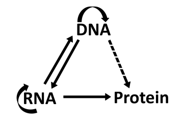
The expanding world of RNA and its implications
Among the macromolecules of life, RNA has a unique distinction- on the one hand, just like DNA, it can serve as genetic material and, on the other, like proteins, it can serve as a catalyst. mRNA, rRNA and tRNA together form the group of “core” RNAs. However, many other types of non-coding RNA (ncRNA) molecules have been discovered and these may be just the “tip of the iceberg” [2060, 2061, 2062, 2063, 2064, 2065, 2066]. Although some of their regulatory functions have been discovered, at present, our understanding of the mechanisms of these processes is far from clear.
Post-transcriptional processing of mRNA
In bacteria freshly polymerized mRNA transcripts can be directly translated into the corresponding proteins. But, in a eukaryotic cell transcription takes place in the nucleus. The mRNA transcript undergoes various types of post-transcriptional “processing” both inside nucleus as well as in the cytoplasm after it is transported out of the nucleus [2067]. One of the distinct features of eukaryotic DNA is the existence of introns, patches of sequences which do not encode for proteins and which, therefore, are removed during splicing of the pre-mRNA. Why did evolution favor insertion of such apparently “useless” introns into the DNA? Several plausible regulatory functions of introns have been hypothesized.
Appendix D Cytoplasmic and internal membranes of a cell
Major molecular component of membranes are lipids. These amphiphilic molecules consist of a hydrophilic head and two hydrophobic tails. For energetic reasons, in aqueous medium, these molecules form bilayers where two oppositely oriented monolayers of lipids stick together with the heads outside and the tails inside the bilayer [2068]. In animal cells, cholesterol is another important component of the cell membrane. From the perspective of molecular transport across the membrane, the membrane proteins are crucially important [2069]. The four-decade old fluid mosaic model [2070, 2071, 2072] is the best representation of the cytoplasmic membrane of animal cells; the molecular details of the membrane is not fairly well understood [2073, 2074].
Gram-positive bacteria have a single plasma membrane that consists of a inner membrane (IM) and a thick outer layer, called cell wall. In contrast, Gram-negative bacteria are enclosed by two membranes where the inner membrane (IM) and the outer membranes (OM) are separated by the periplasmic space that also contains a peptidoglycan layer [2075, 2076]. Based on experimental investigations, it is now generally believed that the first ancestor of all eukaryotes on earth appeared more than 1.5 billion years ago when a bacterial invader cell became captive of the host and became the precursor of present-day mitochondria [2077]. Therefore, it is not surprising that mitochondrial membrane shares many features of Gram-negative bacteria; the inner and outer membranes of each mitochondrion is separated by an intermembrane space [2078]. Because of its important biological functions, which include protein translocation across mitochondrial membranes, it remained an indispensable feature of mitochondria in spite of many other evolutionary changes in the evolution of mitochondria from its bacterial ancestor.
Nuclear envelope and nuclear pore complex (NPC)
The nuclear pore complex (NPC) [2079, 2080, 2081] is a large assembly of more than two dozens of different types of proteins that are collectively called nucleoporins and denoted by the abbreviation Nups. Its shape resembles the upper half of an hourglass. The rim of the channel is sandwiched between the cytoplasmic ring and the nuclear ring. This assembly has a eight-fold symmetry about an axis normal to the plane of the membrane. On the cytoplasmic side of the membrane, eight fibrils extend from the eight lobes which are arranged in the form of a ring. On the nucleoplasmic side of the membrane these eight fibers join to form a basket-like structure. The diameter of the channel is about 60-70 nm at its widest point and about 25-45 nm at its narrowest point. The outer radius of the ring can be as large as 125 nm and the total length of the NPC in the direction perpendicular to the nuclear membrane can vary between 150-200 nm. In addition to the main central channel, the pore can also support some minor peripheral channels.
Appendix E Internal compartments of a cell
| Compartment | Special functional role |
|---|---|
| Nucleus | Repository of genetic material |
| Mitochondria & Chloroplast | Power plant |
| Endoplasmic reticulum | Packaging center |
| Golgi apparatus | Post office |
| Peroxisome | |
| hline |
Diatoms, an unicellular eukaryote, is an example of a special class of organisms that possess both mitochondria and chloroplasts [2082]. In recent years, organelle-like compartments have been discovered also in prokaryotic cells [2083]. However, no counterpart of nucleus has been found so far in prokaryotic cells (see table 13 for internal compartments of eukaryotic cells).
Appendix F Viruses, bacteriophages and plasmids: hijackers or poor parasites?
The concept of virus (including bacteriophages) has an interesting history and its proper definition was a matter of debate even half a century ago [2087, 2088]. A virus is composed of a genome encapsulated within a capsid that is made of proteins [2089]. Different types of viruses differ in size, shape, structure of the capsid and the spatial organization of the genome within it [2090]. Some have an envelope made of lipids whereas others and not enveloped. In contrast to living cells, where the genome is exclusively DNA, viruses can also have RNA as their genetic material. In fact, their genome can be either single-stranded or double-stranded RNA or DNA. Majority of the viruses are, in fact, RNA viruses. Among the RNA viruses, there is a special class with single-stranded RNA genome that are called retrovirus [2091].
The retroviruses not only exploit the machineries of their hosts, but also integrate dsDNA, polymerized from their RNA genome templates, into the genome of the host [2093]. Such DNA sequences integrated into the host genome gets passed onto the daughter cells during division of the virus-infected host. It may become “endogenous viral sequence” [2094, 2095, 2096] in the future generations of the host. The entire life cycle of a virus [2097], including the mechanism of packaging, and the spatial organization of the packaged genome also varies depending on the nature of the genetic material [2098]. Normally, the viral genome encodes the “structural” proteins which are constituents of its capsid. Moreover, it also encodes for some “non-structural” proteins which are essential for the replication of its genome. However, a virus cannot replicate using only the machines at materials at its disposal. Besides, unlike eukaryotic and prokaryotic cells, a virus does not “divide” into “daughter viruses”. Instead, a virus enters a living host cell not only to replicate its genome but also to assemble many copies of itself by exploiting the machineries of the host cell [2099]. The capsid not only protects the viral genome [2100] but also participates in the process whereby the genome infects the host cell. Contrary to the naive expectation, not all viruses are harmful; some viruses develop a symbiosis with their host and are “good” virus for the host [2101].
Plasmids are extrachromosomal DNA in bacterial cells [2102]. These can be replicated just like chromosomal DNA and can be passed to the daughter cells during cell division.
All the eukaryotes, namely, animals, plants (and algae) as well as fungi can be invaded by their respective viruses. Human immunodeficiency virus (HIV), which causes the disease acquired immunodeficiency syndrome (AIDS) [2092], is a retrovirus and is the most dreaded among the viruses that can infect homo sapiens (humans). Among the viruses which can infect plants, an well studied example is the Tobacco mosaic virus .
Bacteriophages are also viruses, but these infect prokaryotes. T-odd (e.g., T7) and T-even (e.g., T4) bacteriophages, phage , , etc. are some of the extensively used model bacteriophages. Not all phages are “tailed” [2104]; filamentous bacteriophages are also widespread [2105, 2106]. Viruses which infect archaea [2107] are called archeovirus [2108].
F.1 Baltimore classification of viruses according to their genome
The viruses have been divided into six different classes each of which has a characteristic distinct method of expressing its genetic information [2109]. An mRNA strand that can be translated directly into a protein is called a (+)mRNA strand. A ssDNA that has the same polarity as the (+)mRNA is called (+)DNA.But, a (+)DNA cannot be transcribed directly into a (+)mRNA. Instead, a complementary DNA strand, called (-)DNA, is directly transcribed into a (+)mRNA. Similarly, on direct replication, a (+)RNA produces a complementary strand that is called a (-)RNA.
Appendix G Organization of packaged genome: from virus and prokaryotes to eukaryotes
The diverse ways in which the genome is organized in different systems [2112] shows the extraordinary richness of life. In every cell the genetic information is encoded in the sequence of the nucleotides. Thus, at some stage of biological evolution, Nature chose an effectively linear device (namely, a NA strand) and a quaternary code (i.e., four symbols, namely, A, T, C, G) for storing genetic information. This was not the most efficient choice! The fewer is the number of letters of the alphabet the longer is the string of letters required to express a given message. Why does nature use exact 4 letters to write the genetic message on nucleic acids? Why does nature use 20 amino acids for making proteins? Are these numbers results of Darwinian evolution which initially could have been different?
One serious consequence of nature’s choice of the memory device and coding system is that even for the most primitive organisms like an E.coli bacterium, the total length of the DNA molecule is orders of magnitude longer than the organism itself! The problem is more acute in case of eukaryotic cells where an even longer DNA has to be accomodated within a tiny nucleus! Moreover, random packaging of the DNA into the nucleus would not be desirable because, for wide variety of biological processes involving DNA, specific segments of the DNA molecules must be “unpacked” and made accessible to the corresponding cellular machineries. Furthermore, at the end of the operation, the DNA must be re-packed. Even in bacteria and viral capsids, the genome has to be packaged in a manner which allows efficient access during various processes of DNA and RNA metabolism.
For detailed accounts of chromosome organization and function see, for example, refs.[2113, 2114, 2115]. A brief summary, appropriate as an introductory reading for uninitiated physicists is available in ref.[2112]
As stated earlier, the viral genomes may consist of DNA or RNA. There are two alternative mechanisms for packaging of the genome. In case of some viruses, the genome is encapsulated by molecules that self-assemble around it. In contrast, the genome of other viruses are packaged into a pre-fabricated empty container, called viral capsid, by a powerful motor.
Nature has solved the problem of packaging genetic materials in the nucleus of eukaryotic cells by organizing the DNA strands in a hierarchical manner and the final packaged product is usually referred to as the chromatin [2116, 2117] The primary repeating unit of chromatin at the lowest level of the hierarchical structure is a nucleosome [2118]. The cylindrically shaped core of each nucleosome consists of an octamer of histone proteins around which 146 base pairs (i.e., nm) of the the double stranded DNA is wrapped about two turns (more precisely, 1.7 helical turns); the arrangement is reminiscent of wrapping of a thread around a spool. There are equispaced sites, at intervals of base pairs (bp), on the surface of the cylindrical spool. Electrostatic attraction between these binding sites on the histone spool and the oppositely charged DNA seems to dominate the histone-DNA interactions which stabilize the nucleosomes. The helical curve formed by the histone-DNA overlap is often referred to as the “footprint” of the DNA.
Appendix H Experimental methods: introduction to the working principles
Experiments play the most important roles in all natural sciences. Throughout this review we use the term ”in-vitro” to mean processes occuring outside living cells whereas the term “in-vivo” is used exclusively for processes occuring inside living cells. Naturally, more controlled experiments are possible in-vitro than in-vivo. In analogy with in-vitro and in-vivo experiments, computer simulation is often referred to as in-silico experiments.
H.1 FRET: tool for monitoring conformational kinetics
Fluorescence is the phenomenon in which a molecule gets excited when illuminated with light of a specific wavelength and, then de-excites by emitting light whose wavelength is usually longer than that of the exciting light. A molecule that is capable of exhibiting the phenomenon of fluorescence is called a fluorophore. Since the wavelength of the emitted light is somewhat longer than that of the light absorbed, the background can be darkened by rejecting the exciting light using appropriate filters. In reality, both the excitation and emission spectra of a molecule have characteristic shapes with a peak and a non-zero width. Therefore, the positions of the peaks of the absorption and emission spectra are identified as the corresponding characteristic frequencies; the larger the difference in these two frequencies the easier it is to record the emission from a fluorophore by filtering out the exciting light.
In general, the desirable properties of fluorophores are as follows:
(i) it should be bright,
(ii) it should, preferably, emit light in the visible region of the spectrum,
(iii) fluctuations in its emission intensity, during the experiment, should be
as small as possible;
(iv) is should be sufficiently small and its interaction with the molecule
under investigation should be weak so that it does not perturb the molecule
under investigation,
(v) it should be available in a form which is suitable for “attachment”
with the molecule under investigation.
Extrinsic fluorescence reporters are usually organic dyes or quantum dots. Intrinsic reporters are genetically engineered in the cell so that a fluorescent molecule forms a part of the protein under investigation; the green fluorescent protein (GFP) and its related cousins with other colors are now used routinely [2119].
FRET (Fluorescence / Förster Resonance Energy Transfer) [2120] is a technique based on a quantum-mechanical phenomenon. It requires two different species of fluorophores called a donor and an acceptor. The donor absorbs laser light at a frequency higher than that of the acceptor. Because of the electromagnetic interactions between the two, non-radiative transfer of energy can take place from the donor to the acceptor if the acceptor is sufficiently close to the donor. Since the efficiency of the process falls with the sixth power of the separation between the two fluorophores, it is significant only when the separation is of the order of O(nm). Such a resonant transfer of excitation energy of the acceptor to the donor excites fluorescence of the acceptor, resulting in a decrease in the fluorescence of the donor. This is a powerful technique for probing the separation between either two different molecules or two different domains of a single macromolecule; the two molecules or the two domains of interest are labelled by the two fluorophores for this investigation (see fig.59).
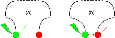
H.2 Optical microscopy: diffraction-limited and beyond
In the fluorescence-based techniques discussed above the kinetics of the molecules are inferred from the pattern of temporal variation of the intensity of the fluorescence. However, seeing is believing. Telescopes opened up the celestial world in front of our eyes. Microscopes aid our vision to “see” the microscopic world of both living and nonliving systems. Naturally, the most direct approach to “see” the molecular machines in its natural environment is to use laser based optical microscopy [2121]. Spectacular progress in optical microscopy over the last two decades [2122] has been possible because of important contributions from several different disciplines; these include, for example, physics (principles of optics), chemistry (synthesis of dyes), genetics (tagging molecules with markers) and engineering (instrumentation and signal processing). However, it is worth uttering a word of caution here: one has to be very careful so as to avoid potential pitfalls in this apparently straightforward approach [2123].
Optical microscopy
Diffraction-limited techniques Sub-diffraction techniques
H.2.1 Diffraction-limited microscopy
The contrast between an object and its background can be enhanced by exploiting the variations in the refractive indices induced, for example, by appropriate staining; these techniques include the phase-contrast microscopy. Fluorescence provides an even better means of enhancing the contrast between the object and its background [2124, 2125, 2126, 2127]. Although fluorescence microscopy is now done routinely, a beginner should be aware of the potential pitfalls [2128].
Magnification makes the observed object bigger, but does not improve spatial resolution which, for conventional optical microscope is limited by a natural constraint. Because of diffraction of light, which is a consequence of its wave nature, image of a point source of light is not a point, but a volume. The corresponding plot of the intensity profile in the image plane is called the point spread function (PSF). Because of the rotational symmetry in the image plane perpendicular to the optic axis, the area in the image plane illuminated by a point source is a circular pattern. The bright circular central patch, called the “Airy disc”, is surrounded concentrically by increasingly darker circles.
According to Abbe’s theory, the spatial resolution of a microscope is half the radius of the first dark circular fringe. Hence, (NA) where the numerical aperture (NA) depends on the refractive index of the medium and the half angular aperture : NA = n sin . The largest value of NA for a good quality microscope and, therefore, using nm, we get .
If the point objects are sufficiently far apart from one another, each forms its own distinct PSF without any overlap with that of another. One can locate the center of the PSF by fitting, e.g., a Gaussian. This center is expected to coincide with the position of the point object that creates this PSF.
Interestingly, Abbe himself speculated in 1876 that “future generations will perhaps find other ways to circumvent the limits imposed by light microscopy, which we consider unsurmountable, by making still unknown processes and forces serve this purpose” [2126].
Recall that one of the assumptions made in the derivation of the Abbe limit is that the two point sources emit light of identical spectral characteristics. But, if the two sources emit lights of different colors, they could be easily resolved by using appropriate filters to reject light from one while localizing the other [2129]. However, success of this route to super-resolution hinges on the ability to label different objects with different types of fluorophores which would emit lights of different colors. For most real problems this is an impractical approach.
H.2.2 Sub-difraction microscopy (or, super-resolution nanoscopy)
The invention of the optical microscopes in the seventeenth century made it possible to have a glimpse of the world of micro-organisms (bacteria, etc.) [2130]. But these microbes are typically micron-size objects. For directly seeing nano-machines, it would be ideal if we could have “nanoscopes” whose resolution surpasses the Abbe limit; however, such “nanoscopes” were not available until recent times [2131, 2132]!
How do the sub-diffraction techniques developed in the last two decades achieve “super-resolution” (i.e., spatial resolution higher than the Abbe limit) [2133, 2129, 2134, 2135, 2136]? We answer this question below by explaining the principles.
Recall that the derivation of the Abbe limit assumed that the two objects emitted light simultaneously leading to the overlap of the two PSFs. But, if only one of these two were fluorescent at a time, each could be localized separately and the full image of the pair could be constructed by superimposing their individual images recorded separately at two different instants of time.
Both the objects can be imaged separately if these are labelled by fluorophores that are photo-switchable, i.e., switched ON (fluorescent) and OFF (non-fluorescent) with appropriately selected laser beams in a sequential manner [2129]. Most of the nanoscopes achieve super-resolution exploiting essentially this simple idea although the details of implementation vary from one technique to another. Stimulated emission depletion (STED) microscopy is based targeted switching whereas stochastic switching is exploited in single-molecule localization microscopy (SMLM) [2137], photo-activated localization microscopy (PALM), stochastic optical reconstruction microscopy (STORM), etc.
H.3 Single-molecule imaging and single-molecule manipulation
Broadly speaking, the single-molecule techniques [2138, 2139, 2140, 2141, 2142] can be classified into two groups: (i) methods of imaging, and (ii) methods of manipulation.
Single-molecule techniques
Single-molecule imaging Single-molecule manipulation
However, combining techniques of manipulation with those of imaging makes it possible to achieve both simultaneously [2143, 2144, 2145].
Fluorescence, which we have already introduced above, has been exploited extensively in imaging single molecules. [2146, 229, 2147, 2148, 2149, 2150, 2151, 2152]. In addition to passive observation under a microscope, spectroscopic analysis of the amplitude, frequency, polarization of the light emitted by the single molecule and their variations in space and time provide useful informations.
For observing effects of chemical manipulations of molecular machines, imaging may be adequate. Several techniques have been developed for for mechanical manipulations of the nanomachines of life [2153, 2154, 2155, 2156, 2157, 2158, 2159].
Mechanical manipulation of a single biomolecule
Mechanical transducers Field-based transducers
SFM Micro-needle EM-field Flow-field
Electric field Magnetic field
The existence of the “gradient” force, which is exploited in setting up an optical trap, was discovered accidentally [2160, 2161]. Consider a dielectric bead exposed to a laser light beam whose intensity is spatially inhomogeneous. The physical origin of the gradient force can be understood easily within the framework of geometrical optics provided ; however, the existence of the gradient force however, does not depend on the validity of this condition.
Mathematical expression for the gradient force has been derived [2162, 2163]. For a guide to the scientific literature on optical tweezer (up to 2003) see ref.[2164]. Several elementary introductions to the basic principles of optical tweezers and their design are available; we mention here only a few of those which are presented in the context of molecular machines [2165, 2166, 2167, 2168, 2169, 2170, 2171].
In magnetic tweezers [2172, 2173], the macromolecule is attached between a surface and a superparamagnetic bead. Stretching force can be applied on the macromolecule by controlled alterations of the external magnetic field. A major advantage of the magnetic tweezer is that the same set up can be used also to apply torque on the molecule by merely rotating the magnetic field.
H.4 Determination of structure: X-ray crystallography and electrom microscopy
X-ray diffraction [2174] and electron microscopy [2175] are two of the most powerful techniques of determination of the structures of molecular machines. Both these techniques provide ensemble-averaged results. Each sample of the molecular machine, when analyzed with X-ray diffraction or electron microscopy, provides essentially a “static” picture. But, informations on time evolutions of structures can also be obtained from X-ray and electron microscopic studies by appropriate protocols for sample preparation and repetitions of the experiments.
X-ray crystallography
The basic principle of X-ray scattering for the determination of the structure of macromolecules is as follows [2176]: an atomic constituent of the macromolecule absorbs some energy of the X-ray incident on it and then re-radiates the same in all directions. A protein crystal has a periodic array of identical atoms. The X-rays re-radiated by these atoms interfere constructively in some directions whereas they interfere destructively in all the other directions. Therefore, the detectors record a “pattern” in the intensity of X-ray scattered by the protein crystal sample. But, such a “diffraction pattern” provides an indirect, and static, image of a molecular machine. X-ray diffraction requires Fourier transform from momentum space to get the structure in real space.
Electron microscopy
Electron microscopy is a powerful alternative for the determination of structures of those macromolecules whose crystals are not available [2175]. The deBroglie wavelength associated with a material particle is given by where is the momentum of the particle. Therefore, a desired short deBroglie wavelength can be attained by accelerating a charged particle to the corresponding required momentum by applying an external electric field. Electrons are ideal for this purpose because an electron beam can also be easily bent and focussed using a suitable magnetic field configuration. But, the generation and control of the electro-magnetic fields makes the electron microscope costly. Moreover, image obtained from an electron microscope requires special expertise to interpret. Often, better results are obtained by a combination of X-ray crystallography and electron microscopy [2177].
Unlike optical microscopes, elaborate preparation of a sample is required before observing under an electron microscope. Keeping the sample hydrated (i.e., “wet”) was a challenge which could be overcome by a technical breakthrough. In this approach, the aqueous sample is cooled very rapidly by plunging it into an appropriate liquid maintained at a sufficiently low temperature. Because of the high rate of cooling, the water surrounding the specimen does not get any opportunity to form ice crystal and, instead, gets “vitrified” (i.e., amorphous). Moreover, because of the low temperature of the vitrified water, nucleation of ice crystals in this metastable medium is highly improbable. Because of the low-temperature techniques used in sample preparation, this technique is called cryo-electron microscopy (cryo-EM) [2178]. The process of reconstruction of the full 3D structure of an object by appropriately combining a series of 2D images recorded from different angles is called cryo-EM tomography. Modern electron microscopy has already provided deep insight into the structure and function of many molecular machines [2179, 2180, 2181, 2182, 2183, 2184, 2185].
Appendix I Modeling of chemical reactions
I.1 Deterministic non-spatial models of chemical reactions: rate equations for bulk systems
At this level, the problem of chemical kinetics can be formulated as follows: suppose a macroscopically uniform mixture of chemical species is confined in a fixed volume and can interact through reaction channels. The main assumption of the rate equation approach is that the population dynamics, formulated in terms of the concentrations of the reactant and product species, is a continuous and deterministic process. For a well stirred chemically reacting bulk system, this is a reasonably good approximation. If the concentrations of all the species are given at some initial instant of time, what will be the corresponding concentrations at any later arbitrary instant of time ? The traditional approach is based on ordinary differential equations, called chemical reaction rate equations, for the concentrations of the molecular species.
In chemical kinetics, the concentration of the -th molecular species is given by the molarity , measured in the number of moles per liter, where is the number of moles of the s-th molecular species. Another related quantity is the molar fraction . Thus, if of all the components in the solution are known, can be obtained. Conversely, if the are known, can be obtained from .
Let us assume that the concentration of the -th molecular species is denoted by a continuous, single-valued function of time . Then, the corresponding chemical rate equations can be expressed as [2186, 2187, 2188]
The specific forms of the functions are determined by the actual nature of the reactions. For example, for the simple first order irreversible reaction
| (287) |
the ordinary differential equations governing the populations of the two molecular species and are
| (288) |
which are usually referred to as the rate equations and the square brackets indicate the respective concentrations. For the first order reversible reaction
| (289) |
the corresponding reaction rate equations are
The coefficients and depend, in general, on the temperature and pressure , etc., but are independent of the concentrations of the reactants and the products. At the level of the chemical rate equations, the rate constants are phenomenological parameters whose numerical values are to be supplied from empirical data. Rate constants usually depend strongly on temperature. An overwhelmingly large number of rate constants are found to vary with temperature according to the Arrhenius equation:
| (291) |
where is called the activation energy (barrier height).
Note that the rate equations (LABEL:eq-rate12) are linear. On the other hand, for the second order reaction
| (292) |
the rate equations
| (293) |
are nonlinear.
I.1.1 Thermodynamic equilibrium, transient kinetics and non-equilibrium steady states
With two examples of very simple reactions we introduce the concepts of transient and equilibrium behavior in the context of chemical reactions. We also demonstrate how transient kinetics can be utilized to estimate the rate constants [2189]. Let us begin with the reaction (287). The concentration of varies with time exponentially:
| (294) |
The slope of the plot of versus yields the rate constant .
Equilibrium constant
Next consider the reaction (289). Any arbitrary initial concentrations and eventually reach the corresponding equilibrium values
| (295) |
In the equilibrium state, the equilibrium constant , defined as
| (296) |
Note that
| (297) |
Thus, the equilibrium constant is a thermodynamic parameter that characterizes the equilibrium state of the reacting system. For a given reaction, the equilibrium constant can be obtained by measuring the concentrations of the reactants and products in equilibrium. The assay need not measure the concentrations chemically; a common alternative is an optical assay where the fluorescence intensities must be proportional to the respective concentrations. In fact, any property, that is proportional to the concentration, can be measured for estimating . In order to avoid possible pitfalls, one has to design the careful experiment and use appropriate protocols [2190].
Transient kinetics
Note that the fact in (LABEL:eq-rate12) reflects the conservation law:
| (298) |
where the total concentration remains constant. From equations (LABEL:eq-rate12) we get
| (299) |
with . Thus, any fluctuation in the populations of the two species decays exponentially with time with an effective time constant to reach the thermodynamic equilibrium values (295). For a reacting system which can attain a state of thermodynamic equilibrium, small deviations from such the equilibrium state are merely transients. However, kinetics of the decay of such transient states can be utilized to measure the rate constants for both the forward and reverse transitions. In this approach, one simply changes the condition of equilibrium of the system and, then, monitors the time-dependent concentrations during the process of re-equilibration. The slope of the plot of yields the sum . Moreover, the can be obtained from (296) provided the equilibrium concentrations and are known.
Non-equilibrium steady-states of chemically reacting systems
The chemical system where the reaction (289) takes place exhibits transient behavior, described by the equation (299), till the system reaches the equilibrium state where the concentrations attain the corresponding time-independent values (295). Thus, in the equilibrium state the concentrations of the reactants and products remain steady (or, stationary). But, not every chemical steady states is an equilibrium state of the system; equilibrium happens to be just a special steady-state. Nonequilibrium steady states (NESS) can exist only in open systems where the system exchanges matter with its environment and consumes energy dissipating part of it as heat [239, 2191, 2192, 2193, 2194]. Biochemical reactions within a living cell are typical examples where such NESS can occur.
As an example, consider the reaction
| (300) |
with a balanced input and output . In this case the equations (LABEL:eq-rate12) are modified to
| (301) |
so that the system reaches a non-equilibrium steady state where
| (302) |
Moreover, defining the forward and reverse fluxes and by the relations
| (303) |
in the non-equilibrium steady state of the system whereas thermodynamic equilibrium demands that , i.e., .
Stoichiometry and reaction rates
Next, let us consider more general complex reactions of the type
| (304) |
where A and B are the reactants while C and D are the products. The stoichiometry of this reaction is such that the rate of formation of one molecule of C (and that of four molecules of D) is equal to the rate of consumption of two molecules of A (or, that of 3 molecules of B). In general, for a reaction like (304) the stoichiometric coefficients if -th species is a product (reactant). Thus for the reaction (304), the stoichiometric coefficients of A,B,C,D are the integers , respectively.
Often a more general notation is used for expressing the rate equations. Suppose denotes is a column vector whose three elements are the concentrations of , and at time for the reaction (292). Then, the rate equations can be recast as
| (305) |
where , and the functions and for the forward and reverse reactions are given by
| (306) |
We define the extent of the reaction as follows: when the chemical reaction advances by , the corresponding changes in the amounts of the reactants and the products in the above mentioned reaction are given by
| (307) |
i.e.,
| (308) |
Any possible ambiguity in the definition of the rate of the reaction is avoided by defining the reaction rate to be , so that, in general, .
If the reaction (304) takes place in the opposite direction, i.e., all the stoichiometric coefficients also reverse their sign and, therefore, flips its sign. Thus, the sign of indicates whether the reaction is proceeding in the forward or the reverse direction; for the forward reaction whereas for the reverse reaction.
The actual extent of a reaction depends on the amount of substance used in the reaction. A better definition of the rate of reaction is where is the volume of the reaction chamber. This definition allows one to associate a single rate with the entire equation corresponding to a reaction. All practical problems of chemical kinetics can be reduced to finding how changes with time . From one can calculate the time evolution of the concentrations of each chemical species involved in the reaction [2186].
I.2 Stochastic non-spatial models of reaction kinetics
The rate equations conceal a great deal of detailed physical processes involved in the reaction. In reality, the time evolution of the populations cannot be continuous because the number of molecules can change only by discrete integers. Moreover, the evolution is not deterministic because it is impossible to predict the exact molecular populations at an arbitrary time unless the positions and velocities of all the molecules in the system, including those in the solvent (i.e., reservoir or bath) are taken into account. Furthermore, the smaller is the population of a reacting species, the stronger are the fluctuations that makes a stochastic description unavoidable. We now develop a theoretical formalism for stochastic chemical kinetics that describes the population dynamics of the reacting species as a discrete, stochastic process that is assumed to evolve in a continuous time.
To our knowledge, one of the earliest studies of stochastic fluctuations in chemical reactions was carried out by Max Delbrück [2195]. The literature on stochastic modeling of (bio-)chemical reactions, including enzyme kinetics, is too vast to be covered in this appendix; only some representative original works of the successive decades [2196, 2197, 2198, 2199, 2200, 2201]. and a few useful reviews [68, 69, 70, 71, 72, 73, 74, 77, 79] are listed in the references. Authors of most of these works were fully aware of the fact that their results on the fluctuations in chemical kinetics would be very relevant in the limit of extremely low concentration of at least one of the reactants. However, their ideas were far ahead of their time! It took a few decades to develop the single molecule techniques with which, for example, single-enzyme experiments are now carried out routinely. Some of the old results can now be tested experimentally while some of the subtle issues raised earlier may get resolved from a modern perspective.
I.2.1 Chemical master equation
Consider chemical species , interacting through reaction channels. Let Number of molecules of the s-th species at time . Our goal is to obtain the state vector , given the state vector , at time .
The stoichiometric coefficients form a matrix whose elements is the stoichiometric coefficient for the s-th species in the r-th reaction. So, if the r-th reaction takes place, the state vector changes to where . We also define the propensity function (transition probabilities per unit time) so that is the probability that the r-th reaction takes place in time interval between and thereby leading to a change of the molecular population . Thus, a given reaction channel is characterized mathematically by two quantities, namely, (i) the state change vector , and (ii) The propensity function .
Let us assume that is so small that no more than one reaction of any kind can take place in the interval between and . Then, we can write the “chemical” master equation [2200, 71, 72, 70]
| (309) |
for the probability .
Gillespie algorithm
Except for a few special reactions
[2202],
in general, it is very difficult
(practically impossible) to solve the CME either analytically or
numerically. Therefore, it is often investigated following an approach
which is essentially equivalent to Monte Carlo simulation of the
reaction. Gillespie algorithm [2200, 71, 72]
is the most popular technique for simulating the CME. There are
essentially three substeps in each step of this algorithm:
(i) it generates the time step till the next reaction;
(ii) it randomly picks up one of the reactions for its execution;
(iii) it implements the execution of the reaction by advancing the
time by and by updating the number of molecules to reflect
the occurrence of the reaction. Several different variants of this
algorithm and its extensions have been developed in the last three
decades.
Deterministic limit: chemical rate equation from CME
The steps in the systematic derivation of the deterministic chemical reaction rate equations from the corresponding stochastic CME have been clearly stated and the approximating assumptions have been clarified [2203, 2204]. The rate equations for a chemically reacting system can be derived from the corresponding master equations. Let us define the average population by
| (310) |
It is straightforward to derive the rate equation
| (311) |
satisfied by .
I.2.2 Chemical Langevin and Fokker-Planck equations
Suppose the -th component of the -component column vector denote the number of molecules of species at time . Then, the chemical Langevin equation (CLE) [2205, 2206] is given by [236, 75]
| (312) |
The first term directly corresponds to the right hand side of the rate equation except for the fact that denotes the numbers of molecules whereas is the concentration of the molecules of -th species. The second term on the right hand side of (312) adds Gaussian noise of vanishing mean and unit variance.
The CLE is formulated as the kinetics of an individual based model. Just as in the case of Brownian mechanics, an alternative, but equivalent, approach was developed in terms of the chemical Fokker-Planck equation (CFPE) which described the kinetics in terms of populations [75]. However, since this is hardly ever used in the context of molecular motors we’ll not discuss it here.
I.3 Enzymatic reactions: regulation by physical and chemical means
Enzymes are proteins and function as biological catalysts [244]. These are specific in the sense that a specific catalyst speeds up a specific reaction by a factor of to . In spite of common essential features, there are also important differences between non-biological catalysts and enzymes; the most important differences arise from the macromolecular character of the proteins [2207]. The evolution of the structural designs of enzymes from the primitive (presumably inorganic) catalysts and optimization of their performance during various stages of biological evolution are interesting subjects of investigation [2208, 2209] which, however, will not be discussed here.
Enzymatic reactions, which are of major interest here in the context of molecular motors, can be regulated (i) by physical means, or (ii) by chemical means. Physical means include temperature, force, etc. while chemical means depend on interaction of the enzyme with other molecules.
Chemical regulation of an enzyme can be carried out following two different approaches: (a) by regulating the quantity of the enzyme through control on its production, or degradation (or, permanent inactivation by irreversible covalent modification), and (b) controlling the enzymatic activity (of a given amount of enzyme) by its binding and dissociation with small molecules. Any small molecule which can bind an enzyme reversibly is called a ligand. A ligand can be an activator or inhibitor of the enzymatic activity [2207]. Many enzymes need a cofactor for enzymatic activity, the cofactor can be a metal ion or an organic molecule.
Appendix J Elastic stiffness of polymers
DNA, RNA and proteins are linear polymers. These polymers not only introduced a new length scale (characterized by its size) and a time scale (associated with its dynamics) but also brought in its “flexibility” which is not possible with only small molecules. This flexible nature of macromolecules also gives rise to the importance of conformational entropy. In fact, many biological processes are driven by entropic elasticity. Apriori, it is not at all obvious that the phenomenological concepts of classical theory of elasticity, which were developed for macroscopic objects, should be applicable even for single molecules of DNA, RNA, etc. Technological advances over the last two decades made it possible to stretch, bend and twist a single macromolecule and the corresponding moduli of elasticity have been measured [2210, 2211, 2212, 2213, 2214, 2215, 2216, 2217, 2218, 2219, 2220].
The elasticity of nucleic acids is of particular significance because most often genome (DNA or RNA) are stored in bent conformation [2221]. For example, in eukaryotic cells, DNA is bent and wrapped around histones [2222]. Similarly, in viral capsids, nucleic acids are strongly bent for efficient packaging. Furthermore, temporary bending of macromolecules take place in many biological processes driven by molecular motors. Stiff polymers can also play the role of a nano-piston. Therefore, the elasticity of the macromolecules of life is also interesting in the study of molecular machines which polymerize, manipulate and degrade these molecules.
J.0.1 Freely jointed chain model and entropic elasticity
Let us model a linear polymer of monomers, each of length . Freely jointed chain (FJC) model is based on the assumption that the relative orientation between the successive monomers is completely random and does not involve any energy change. Thus, the FJC model is essentially equivalent to a random walk. Therefore, for one-dimensional FJC with a given and end-to-end distance , the entropy is given by
| (313) |
For sufficiently large and , using Stirling approximation, the force exerted by the FJC is found to be where the effective spring constant is
| (314) |
This spring-like behevior of the FJC is of entropic origin.
J.0.2 Worm-like chain and its relation with freely jointed chain: persistence length
The polymer is represented by a flexible chain where an energy cost has to be paid for its bending. Suppose is the unit tangent to the chain at . It turns out that the tangent-tangent correlation function decays exponentially, i.e,
| (315) |
with the arc length . The persistence length of the polymer increases with the increasing bending stiffness whereas it decreases with increasing temperature.
Appendix K Cytoskeleton: beams, struts and cables
The mechanical properties of the cell depends on its cytoskeleton The cytoskeleton of an eukaryotic cell maintains its architecture [2223, 2224, 2126, 2225]. The cytoskeleton is a complex dynamic network that can change in response to external or internal signals. The cytoskeleton is also responsible for intra-cellular transport of packaged molecular cargoes as well as for the motility of the cell as a whole. The cytoskeleton plays crucially important role also in cell division and development of organisms. The cytoskeleton of not only animals, but also those of plants and algae [2226, 2227, 2228, 2229, 2230] as well as those of fungi [2231, 2232, 2233] have been investigated widely (see Table 14). Counterparts of some molecular components of the eukaryotic cytoskeleton have been discovered recently also in prokaryotic cells [2234, 2235, 2236, 2237, 2238, 2239, 2240, 2241, 2242, 2243, 2244, 2245, 2246].
K.1 Cytoskeleton of eukaryotic cells
The protein constituents of the cytoskeleton of eukaryotic cells can be broadly divided into the following three categories: (i) Filamentous proteins, (ii) accessory proteins, and (iii) motor proteins. The three classes of filamentous proteins, which form the main scaffolding of the cytoskeleton, are: (a) actin, (b) microtubule, and (c) intermediate filaments.
The three superfamilies of motor proteins are:
(i) myosin superfamily,
(ii) kinesin superfamily, and
(iii) dynein superfamily.
Both kinesins and dyneins move on microtubules; in contrast, myosins
either move on actin tracks or pull the actin filaments.
| Category | Member |
|---|---|
| Filamentous protein | Actin |
| Filamentous protein | Microtubule |
| Filamentous protein | Intermediate filaments |
| Accessory protein | Filament polymerization regulators |
| Accessory protein | Filament-filament linkers |
| Accessory protein | Filament-plasma membrane linkers |
| Motor protein | Myosin |
| Motor protein | Kinesin |
| Motor protein | Dynein |
On the basis of functions, accessory proteins can be categorized as follows: (i) regulators of filament polymerization, (ii) filament-filament linkers, (iii) filament-plasma membrane linkers. Among the regulators of filament polymerization, some promote nucleation of a filament, while some other species cap a filament thereby terminating its growth. Some regulators enhance the rate of filament growth whereas some others are involved in the depolymerization and severing of filaments. Filament-filament cross-linkers organize higher-order assemblies and networks of the filaments.
Microtubules are cylindrical hollow tubes whose diameter is approximately 20 nm. The basic constituent of microtubules are globular proteins called tubulin. Hetero-dimers, formed by and tubulins, assemble sequentially to form a protofilament. 13 such protofilaments form a microtubule. The length of each dimer is about 8 nm. Since there is only one binding site for a motor on each dimeric subunit of MT, the minimum step size for kinesins and dyneins is 8 nm.
Although the protofilaments are parallel to each other, there is a small offset of about 0.92 nm between the dimers of the neighboring protofilaments. Thus, total offset accumulated over a single looping of the 13 protofilaments is which is equal to the length of three dimers joined sequentially. Therefore, the cylindrical shell of a microtubule can be viewed as three helices of monomers. Moreover, the asymmetry of the hetero-dimeric building block and their parallel head-to-tail organization in all the protofilaments gives rise to the polar nature of the microtubules. The polarity of a microtubule is such an tubulin is located at its - end and a tubulin is located at its + end.
Filamentous actin are polymers of globular actin monomers. Each actin filament can be viewed as a double-stranded, right handed helix where each strand is a single protofilament consisting of globular actin. The two constituent strands are half staggered with respect to each other such that the repeat period is 72 nm.
Appendix L Kinetics of nucleation, polymerization and depolymerization of polar filaments: treadmilling and dynamic instability
Polymerizing and depolymerizing polar filaments generate force by mechanisms that we discuss in detail in several sections of this review. The role of -tubulin in the nucleation of MT filaments has been known for quite some time [2247, 2248, 2249]. Theoretical models have been developed for the kinetics of MT nucleation [2250, 2251, 2252, 2253]. Two classes of actin nucleating proteins are: (i) formin protein family; and (ii) Arp2/3 complex [2254, 2255, 2256].
The dynamics of polymerization and depolymerization of microtubules is quite different from those of most of the common proteins. Dynamic instability [2257, 2258, 2259, 2260] is now accepted as the dominant mechanism governing the dynamics of microtubule polymerization. Each polymerizing microtubule persistently grows for a prolonged duration and, then makes a sudden transition to a depolymerizing phase; this phenomenon is known as “catastrophe”. However, the rapid shrinking of a depolymerizing microtubule can get arrested when it makes a sudden reverse transition, called “rescue”, to a polymerizing phase.
There are strong experimental evidences that the dynamic instability of a MT is triggered by the loss of its guanosine triphoshate (GTP) cap because of the hydrolysis of GTP into guanosine diphosphate (GDP). Although the detailed mechanism, i.e., how the chemical process of cap loss induces mechanical instability, remains far from clear, kinetic models have been developed based on plausible mechanisms [2261, 2262, 2263, 2264, 2265].
Some small molecules can suppress the dynamic instability and infuence the rates of growth and/or shrinkage of the microbules when bound to the tubulins. These molecules are potential anti-cancer drugs because of the corresponding implications of the dynamic instability in cell division [2266, 2267, 2268]. Quantitative effects of such drug molecules on the kinetics of MT polymerization /depolymerization and the distribution of the microtubule lengths have been investigated [2269].
Pioneering theoretical model of MT polymerization [2270, 2271, 2272, 2273] and many of their more recent extensions [2274, 2275, 2276, 2277, 2278, 2269, 2263] treated each MT as an essentially one-dimensional object and and without assuming any explicit scenario that causes catastrophe and rescue. An one-dimensional model for the polymerization / depolymerization kinetics of MT, incorporating catastrophe and rescue, was developed by Hill [2270]. In this original version the kinetics is formulated in terms of, effectively, infinite number of coupled ordinary differential equations for , the probability of finding a filament consisting of subunits ( being discrete) at time in the growing (+) and shrinking (-) phases. In a later work, Dogterom and Leibler [2274] described the kinetics in terms of two coupled partial differential equations for where , the length of a MT, is assumed to be a continuous variable. However, more recent works on the kinetics of dynamic instability capture the fact that a MT is a tubular object consisting of 13 protofilaments.
Instead of dynamic instability, it is the treadmilling [2279] that dominates the kinetics of polymerization / depolymerization of actin. Kinetic models of actin polymerization should model it as double-stranded, and capture the effects of ATP hydrolysis [2280, 2281, 2282, 2283]. For a deeper insight into the contrasting features of the polymerization kinetics of MT and F-actin, see [2284].
Acknowledgements:
It is my great pleasure to thank all my students and collaborators for enjoyable collaborations on molecular motors. I sincerely thank John Bechhoefer, Zvonimir Dogic, Arnold Driessen, Pierre Gaspard, Manoj Gopalakrishnan, Steven P. Gross, Hermann-Georg Holzhütter, Mandar Inamdar, Ambarish Kunwar, Charles Lindemann, Roop Mallik, Amit Mitra, Alex Mogilner, Raja Paul, Hong Qian, Andreas Schadschneider, Sean Sun, Andrej Vilfan, Jianhua Xing, Alexey Zaikin and an anonymous referee for their comments and suggestions on various sections of the manuscript. I am indebted to Joachim Frank for many enlightening correspondences and discussions as well as for his patient critical reading of an earlier preliminary shorter version of this manuscript. I thank Ashok Garai, Jeffrey Moffitt and Ajeet Sharma for their comments on earlier shorter drafts of this review and Ajeet Sharma for technical help in producing two figures. Over the last few years, I have also benefitted from many discussions and/or correspondences with Veronika Bierbaum, Stephan Grill, Joe Howard, Frank Jülicher, Stefan Klumpp, Reinhard Lipowsky, Sriram Ramaswamy and Ajay Sood. This work has been supported at IIT Kanpur by the Dr. Jag Mohan Garg Chair professorship and by Department of Biotechnology, government of India. Work on this review was in progress over the last five years during which I have enjoyed the hospitality of several research institutions. Parts of the literature survey for this review were carried out at those institutions, particularly, the Max-Planck Institute for the Physics of Complex Systems (MPI-PKS), Dresden, Germany, University of Cologne, Germany, and the Mathematical Biosciences Institute (MBI) at the Ohio State University, Columbus, USA. These visits have been supported by the Visitors Program of the MPI-PKS (in Dresden), Alexander von Humboldt Foundation (in Cologne) and by MBI and the National Science Foundation under grant DMS 0931642 (in Columbus).
References
- [1] B. Alberts et al.Molecular Biology of the Cell, 5th edition, Garland(2007).
- [2] H. Lodish et al. Molecular Cell Biology, 7th edition, Freeman, (2012).
- [3] L. von Bertalanffy, The theory of open systems in physics and biology, Science 111, 23-29 (1950).
- [4] W. B. Cannon, The wisdom of the body, (Norton, 1932).
- [5] G. Recordati and T.G. Bellini, A definition of internal constancy and homeostasis in the context of non-equilibrium thermodynamics, Exp. Physiol. 89, 27-38 (2004).
- [6] M. Piccolino, Biological machines: from mills to molecules, Nature Rev. Mol. Cell Biol. 1, 149-153 (2000).
- [7] B. Alberts, The cell as a collection of protein machines: preparing the next generation of molecular biologists, Cell 92(3), 291-294 (1998).
- [8] T.D. Pollard, Proteins as machines, Nature 355, 17-18 (1992).
- [9] C. Mavroidis, A. Dubey and M.L. Yarmush, Molecular Machines, in: Annual Rev. Biomed. Engg., 6, 363-395 (2004).
- [10] A. Baumgaertner, Biomolecular machines, in: Handbook of Theor. and Comp. Nanotechnol., ed. M. Rieth and W. Schommers, 1, 1-89 (2005).
- [11] D.S. Goodsell, The machinery of life, 2nd edn. (Springer, 2009).
- [12] N. Cozzarelli, G.J. Cost, M. Nöllmann, T. Viard and J.E. Stray, Giant proteins that move DNA: bullies of the genomic playground, Nat. Rev. Mol. Cell Biol. 7, 580-588 (2006).
- [13] L. Rittie and B. Perbal, Enzymes used in molecular biology: a useful guide, J. Cell Commun. Signal. 2, 25-45 (2008).
- [14] W.M. Stark, B.F. Luisi and R.P. Bowater, Machines on genes: enzymes that make, break and move DNA and RNA, Biochem. Soc. Trans. 38, 381-383 (2010).
- [15] M.F. Carlier, E. Helfer, R. Wade and F. Haraux, Living nanomachines, in: Nanoscience, eds. P. Boisseau et al. (Springer, 2010).
- [16] J. Frank, (ed.) Molecular machines in biology: workshop of the cell (Cambridge University Press, 2011).
- [17] B. Roux, (ed.) Molecular machines, (World Scientific, 2011).
- [18] M.G. Rossmann and V.B. Rao, (eds.) Viral molecular machines, eds. M.G. Rossmann and V.B. Rao (Vol.726 of Adv. Expt. Med. and Biol.), (Springer, 2012).
- [19] J. Howard, Mechanics of motor proteins and the cytoskeleton, (Sinauer Associates, Sunderland, 2001).
- [20] R.D. Vale, Millennial musings on molecular motors, Trends in Cell Biol. 9, Trends in Biochem. Sci. 24, and Trends in Genet. 15 (1999).
- [21] R.D. Vale and R.A. Milligan, The way things move: looking under the hood of molecular motor proteins, Science 288, 88-95 (2000).
- [22] M. Schliwa, (ed.) Molecular Motors, (Wiley-VCH, 2003).
- [23] D. D. Hackney and F. Tanamoi, The Enzymes, vol.XXIII Energy Coupling and Molecular Motors (Elsevier, 2004).
- [24] J.M. Squire and D.A.D. Parry, Fibrous proteins: muscle and molecular motors, (Elsevier 2005).
- [25] T. Duke, Modelling motor protein systems, in: Physics of bio-molecules and cells, eds. H. Flyvbjerg, F. Jülicher, P. Ormos and F. David, 95-144 (Springer, 2002).
- [26] A.B. Kolomeisky and M.E. Fisher, Molecular motors: a theorist’s perspective, Annu. Rev. Phys. Chem. 58, 675-695 (2007).
- [27] H. Wang, Several issues in modeling molecular motors, J. Comp. and Theor. Nanosci. 5, 1-35 (2008).
- [28] A. Goel and V. Vogel, Harnessing biological motors to engineer systems for nanoscale transport and assembly, Nat. nanotechnol. 3, 465-475 (2008).
- [29] J. Howard, Molecular mechanics of cells and tissues, Cellular and Molecular Bioengineering 1, 24-32 (2008).
- [30] D. Chowdhury, Resource Letter PBM-1: Physics of biomolecular machines, Amer. J. Phys. 77, 583-594 (2009).
- [31] W. Hwang and M.J. Lang, mechanical design of translocating motor proteins, Cell Biochem. Biophys. 54, 11-22 (2009).
- [32] C. Veigel and C.F. Schmidt, Moving into the cell: single-molecular studies of molecular motors in complex environments, Nat. Rev. Mol. Cell Biol. 12, 163-176 (2011).
- [33] Q. Cui, Theoretical and computational studies of vectorial processes in biomolecular systems, Theor. Chem. Acc. 116, 51-59 (2006).
- [34] W. P. Jencks, The utilization of binding energy in coupled vectorial processes, in: Adv. Enzymology and Related Areas of Molecular Biology, ed. A. Meister, 51, 75-106 (John Wiley, 1980).
- [35] R. M. Krupka, Channelling free energy into work in biological processes, Exp. Physiology 83, 243-251 (1998).
- [36] P. Mitchell, Foundations of vectorial metabolism and osmochemistry, Bioscience Rep. 11, 297-346 (1991).
- [37] F. M. Harold, Molecules into cells: specifying spatial architecture, Microbiol. Mol. Biol. Rev. 69, 544-564 (2005).
- [38] J.D. Aitchison and T. Galitski, Inventories to insights, J. Cell Biol. 161, 465-469 (2003).
- [39] J. Shrager, The fiction of function, Bioinformatics 19, 1934-1936 (2003).
- [40] G.F.R. Ellis, D. Noble and T. O’Connor, Top-down causation: an integrating theme within and across the sciences, Interface Focus 2, 1-3 (2012); see also other articles in this theme issue on top-down causation.
- [41] E. Mayr, Cause and effect in biology: kinds of causes, predictability, and teleology are viewed by a practicing biologist, Science 134, 1501-1506 (1961).
- [42] K.N. Laland, K. Sterelny, J. Odling-Smee, W. Hoppitt and T. Uller, Cause and effect in biology revisited: Is Mayr’s proximate-ultimate dichotomy still useful?, Science 334, 1512-1516 (2011).
- [43] F. Mazzocchi, Complementarity in biology, EMBO Rep. 11, 339-344 (2010).
- [44] N. Tinbergen, On aims of ethology, Zeits. Tierpsychologie 20, 410-433 (1963).
- [45] A.D. Purushotham and R. Sullivan, Darwin, medicine and cancer, Annals of Oncology 21, 199-203 (2010).
- [46] F. Jacob, Evolution and tinkering, Science 196, 1161-1166 (1977).
- [47] T. Dobzhansky, Nothing in biology makes sense except on the light of evolution, The Amer. Biol. Teacher 35, 125-129 (1973).
- [48] A. Szent-Gyorgyi, The development of bioenergetics, Bioenergetics 3, 1-4 (1972).
- [49] G.A. Parker and J.M. Smith, Optimality theory in evolutionary biology, Nature 348, 27-33 (1990).
- [50] B. Penders, K. Horstman and R. Vos, Walking the line between lab and computation: the “moist” zone, Bioscience 58, 747-755 (2008).
- [51] D. J. Barnes and D. Chu, Introduction to modeling for biosciences, (Springer, 2010), particularly chapters 1, 6 and 7.
- [52] J. M. Epstein, Why model?, Bastille Day Keynote address, Second World Congress on Social Simulation, George Mason University, (2008).
- [53] A. D. Lander, The edges of understanding, BMC Biology 8, 40 (2010).
- [54] J.E. Bailey, Mathematical modeling and analysis in biochemical engineering: past accomplishments and future opportunities, Biotechnol. Prog. 14, 8-20 (1998).
- [55] D.A. Beard, J. B. Bassingthwaighte and A.S. Greene, Computational modeling of physiological systems, Physiol. Genomics 23, 1-3 (2005).
- [56] A. Mogilner, R. Wollman and W.F. Marshall, Quantitative modeling in cell biology: what is it good for?, Developmental Cell 11, 279-287 (2006).
- [57] M.D. Laubichler and G.B. Müller, Models in theoretical biology, in: Modelling Biology: structures, behavior, evolution, eds. M.D. Laubichler and G.B. Müller (MIT Press, 2007).
- [58] D.C. Krakauer, J.P. Collins, D. Erwin, J.C. Flack, W. Fontana, M.D. Laubichler, S.P. Prohaska, G.B. West and P.F. Stadler, The challenges and scope of theoretical biology, J. Theor. Biol. 276, 269-276 (2011).
- [59] A.C. Oates, N. Gorfinkiel, M. Gonzalea-Gaitan and C.P. Heisenberg, Quantitative approaches in developmental biology, Nat Rev. Genetics 10, 517-530 (2009).
- [60] J. E. Cohen, Mathematics is biology’s next microscope, only better; biology is mathematics’ next physics, only better, PLoS Biol. 2, e439 (2004).
- [61] Y. Lazebnik, Can a biologist fix a radio?- or, what I learned while studying apoptosis, Cancel Cell 2, 179-182 (2002).
- [62] P. Hunter and P. Nielsen, A strategy for integrative computational physiology, Physiology 20, 316-325 (2005).
- [63] S.S. Andrews and A.P. Arkin, Simulating cell biology, Curr. Biol. 16, R523-R527 (2006).
- [64] S. Schnell, R. Grima and P.K. Maini, Multiscale modeling in biology, Amer. Scientist 95, 134-142 (2007).
- [65] S. N. Yaliraki and M. Barahone, Chemistry across scales: from molecules to cells, Phil. Trans. Roy. Soc. A 365, 2921-2934 (2007).
- [66] D. Noble, The rise of computational biology, Nat. Rev. Mol. Cell Biol. 3, 460-463 (2002).
- [67] J. Fisher and T.A. Henzinger, Executable cell biolgy, Nat. Biotechnol. 25, 1239-1249 (2007).
- [68] D.A. McQuarrie, Stochastic approach to chemical kinetics, J. Appl. Prob. 4, 413-478 (1967).
- [69] P. Erdi and J. Toth, Mathematical models of chemical reactions: Theory and applications of deterministic and stochastic models, (Princeton university press and Manchester unversity press, 1989).
- [70] T.E. Turner, S. Schnell and K. Burrage, Stochastic approaches for modelling in vivo reactions, Comp. Biol. and Chem. 28, 165-178 (2004).
- [71] D.T. Gillespie, Stochastic chemical kinetics, in: Handbook of materials modeling, ed. S. Yip (Springer, 2005).
- [72] D.T. Gillespie, Stochastic simulation of chemical kinetics, Annu. Rev. Phys. Chem. 58, 35-55 (2007).
- [73] C. Gadgil, Stochastic modeling of biological reactions, J. Ind. Inst. Sci. 88, 45-55 (2008).
- [74] S.X. Sun, G. Lan and E. Atilgan, Stochastic modeling methods in cell biology, Methods in Cell Biol. 89, 601-621 (2008).
- [75] S.S. Andrews, T. Dinh and A.P. Arkin, Stochastic models of biological processes, in:Encyclopedia of complexity and system science, ed. R. Meyers, 9, 8730-8749 (2009).
- [76] D.J. Wilkinson, Stochastic modelling for quantitative description of heterogeneous biological systems, Nat. Rev. Genet. 10, 122-133 (2009).
- [77] M. Ullah and O. Wolkenhauer, Stochastic approaches in systems biology, Wiley Interdisciplinary Reviews on Systems Biology and Medicine 2, 385-397 (2010).
- [78] W.W. Chen, M. Niepel and P.K. Sorger, Classic and contemporary approaches to modeling biochemical reactions, Genes Dev. 24, 1861-1875 (2010).
- [79] H. Qian, Cooperativity in cellular biochemical processes: noise-enhanced sensitivity, fluctuating enzyme, bistability with nonlinear feedback, and other mechanisms for sigmoidal responses, Annu. Rev. Biophys. 41, 179-204 (2012).
- [80] E.O. Voit, Models-of-data and models-of-processes in the post-genomic era, Math. Biosci. 180, 263-274 (2002).
- [81] D. Balding, Inference in complex systems, JRS Interface Focus 1, 805-806 (2011); see also the other articles in the same special issue of JRS Interface Focus on statistical inference.
- [82] E.J. Chikofsky, J.H.Cross II, Reverse engineering and design recovery: a taxonomy, IEEE Software 7(1), 13-17 (1990).
- [83] M.E. Cseste and J.C. Doyle, Reverse engineering of biological complexity, Science 295, 1664-1669 (2002).
- [84] J.R. Platt, Strong inference, Science 146, 347-353 (1964).
- [85] D.A. Beard and M.J. Kushmerick, Strong inference for systems biology, PLoS Comp. Biol. 5, e1000459 (2009).
- [86] T.C. Chamberlin, The method of multiple working hypotheses, Science 15, 92-96 (1890); reprinted in Science 148, 754-759 (1965).
- [87] D.B. kell and S.G. Oliver, Here is the evidence, now what is the hypothesis? The complementary roles of inductive and hypothesis-driven science in the post-genomic era, Bioessays 26, 99-105 (2003).
- [88] L.H. Hartwell, J.J. Hopfield, S. Leibler and A.W. Murray, From molecular to modular cell biology, Nature 402, C47-C52 (1999).
- [89] J.A. Bolker, Modularity in development and why it matters to evo-devo, Amer. Zool. 40, 770-776 (2000).
- [90] J.D.J. Han, Understanding biological functions through molecular networks, Cell Res. 18, 224-237 (2008).
- [91] A.L. Barabasi and Z.N. Oltavi, Network biology: understanding the cell’s functional organization, Nat. Rev. Genet. 5, 101-113 (2004).
- [92] H. Kitano, Biological robustness, Nat. Rev. Genet. 5, 826-837 (2004).
- [93] K.P. Hofmann, C.M.T. Spahn, R. Heinrich and U. Heinemann, Building functional modules from molecular interactions, Trends in Biochem. Sci. 31, 497-508 (2006).
- [94] H. Kitano, Computational systems biology, Nature 420, 206-210 (2002).
- [95] N. Wingren and D. Botstein, Back to the future: education for system-level biologists, Nat. Rev. Mol. Cell Biol. 7, 829-832 (2006).
- [96] F.J. Bruggeman and H.V. Westerhoff, The nature of systems biology, Trends Microbiol. 15, 45-50 (2006).
- [97] D. Noble, Biophysics and systems biology, Phil. Trans. Roy. Soc. A 368, 1125-1139 (2010).
- [98] M.A. O’Malley and O.S. Soyer, The roles of integration in molecular systems biology, Stud. Hist. Phil. Biol. Biomed. Sci. 43, 58-68 (2012).
- [99] P.J. Hunter and T.K. Borg, Integration from proteins to organs, Nat. Rev. Mol. Cell Biol. 4, 237-243 (2003).
- [100] Editorial in Nature Immunology 12 (10) 915 (2011).
- [101] T. Dobzhansky, Biology, molecular and organismic, Amer. Zoologist 4, 443-452 (1964).
- [102] S. J. Gould, Wonderful life: the burgess shale and the nature of history, (W.W. Norton, 1989).
- [103] H.C. Berg, Random walks in biology, (Princeton University Press, 1993).
- [104] R. Phillips, J. Kondev and J. Theriot, Physical Biology of the Cell, (Garland Science, 2009).
- [105] E.M. Purcell, Life at low Reynolds number, Am. J. Phys. 45, 3-11 (1977).
- [106] J.P. Brody, P. Yager, R.E. Goldstein and R.H. Austin, Biotechnology at low Reynolds numbers, Biophys. J. 71, 3430-3441 (1996).
- [107] D’Arcy Thompson, On Growth and Form, vol.I reprinted 2nd edition (Cambridge University Press, 1963).
- [108] F.C. Mackintosh and C.F. Schmidt, Active cellular materials, Curr. Opin. Cell Biol. 22, 29-35 (2010).
- [109] U. Seifert, Stochastic thermodynamics, fluctuation theorems, and molecular machines, Rep. Prog. Phys. 75, 126001 (2012).
- [110] F. Jülicher, Statistical physics of active processes in cells, Physica A 369, 185-200 (2006).
- [111] R.S. Berry, V.A. Kazanov, S. Sieniutycz, Z. Szwast and A.M. Tsirlin, Thermodynamic optimization of finite-time processes, (Wiley, 2000).
- [112] A. Katchalsky and P.F. Curran, Nonequilibrium thermodynamics in biophysics, (Harvard university press, 1967).
- [113] W. Bialek, Noise isn’t negligible (unpublished).
- [114] M.S Samoilov, G. Price and A. P. Arkin, From fluctuations to phenotypes: the physiology of noise, Science STKE 366, re17 (2006).
- [115] E. Paluch, J. van der Gucht and C. Sykes, Cracking up: symmetry breaking in cellular systems, J. Cell Biol. 175, 687-692 (2006).
- [116] special “Perspectives on Symmetry Breaking in Biology”, Cold Spring Harb. Perspect. Biol. (2010).
- [117] K.C. Vermeulen, G.J.M. Stienen and C.F. Schmidt, Cooperative behavior of molecular motors, J. Muscle Res. and Cell Mot. 23, 71-79 (2002).
- [118] R. Mallik and S.P. Gross, Molecular motors: strategies to get along, Curr. Biol. 14 R971-R982 (2004).
- [119] W. F. Marshall, Cellular length control systems, Annu. Rev. Cell Dev. Biol. 20, 677-693 (2004).
- [120] W.F. Marshall, Engineering design principles for organelle size control systems, Sem. Cell dev. Biol. 19, 520-524 (2008).
- [121] Y.M.Chan and W.F. Marshall, Scaling properties of cell and organelle size, Organogenesis 6, 88-96 (2010).
- [122] W.F. Marshall, Origins of cellular geometry, BMC Biol. 9, 57 (2011).
- [123] Y.M. Chan and W.F. Marshall, How cells know the size of their organelles, Science 337, 1186-1189 (2012).
- [124] M. Kirschner, J. Gerhart and T. Mitchison, Molecular vitalism, Cell 100, 79-88 (2000).
- [125] E. Karsenti, Self-organization in cell biology: a brief history, Nat. Rev. Mol. Cell Biol. 9, 255-262 (2008).
- [126] E. F. Keller, Organisms, machines, and thunderstorms: a history of self-organization, part one, Hist. Stud. Natural sci. 38, 45-75 (2008).
- [127] E. F. Keller, Organisms, machines, and thunderstorms: a history of self-organization, part two, Hist. Stud. Natural sci. 39, 1-31 (2009).
- [128] A. Kurakin, Scale-free flow of life: on the biology, economics, and physics of the cell, Theor. Biol. and Med. Modelling, 6, 6 (2009).
- [129] A. Kurakin, Order without design, Theor. Biol. and Med. Modelling 7: 12 (2010).
- [130] T. Misteli, The concept of self-organization in cellular architecture, J. Cell Biol. 155, 181-185 (2001).
- [131] J.D. Halley and D.A. Winkler, Consistent concepts of self-organization and self-assembly, Complexity 14, 10-17 (2008).
- [132] D.J. Wales, Energy landscapes, (Cambridge University Press, 2003).
- [133] K. Henzler-Wildman and D. Kern, Dynamic personalities of proteins, Nature 450, 964-972 (2007).
- [134] D.J. Wales and T.V. Bogdan, Potential energy and free energy landscapes, J. Phys. Chem. B 110, 20765-20776 (2006).
- [135] D.J. Wales, Energy landscapes: calculating pathways and rates, International rev. Phys. Chem. 25, 237-282 (2006).
- [136] P.C. Whitford, K.Y. Sanbonmatsu and J.N. Onuchic, Biomolecular dynamics: order-disorder transitions and energy landscapes, Rep. Prog. Phys. 75, 076601 (2012).
- [137] J.M. Scholey, Compare and contrast the reaction coordinate diagrams for chemical reactions and cytoskeletal force generators, Mol. Biol. Cell 24 433-439 (2013).
- [138] O. Wolkenhauer, M. Ullah, P. Wellstead and K.H. Cho, The dynamic systems approach to control and regulation of intracellular networks, FEBS Lett. 579, 1846-1853 (2005).
- [139] S. Leibler and D.A. Huse, Porters versus rowers: a unified stochastic model of motor proteins, J. Cell Biol. 121, 1357-1368 (1993).
- [140] J. Howard and A.A. Hyman, Microtubule polymerases and depolymerases, Curr. Opin. Cell Biol. 19, 31-35 (2007).
- [141] A. Zemel and A, Mogilner, Motor-induced sliding of microtubule and actin bundles, Phys. Chem. Chem. Phys. 11, 4821-4833 (2009).
- [142] Y. Lecarpentier, D. Chemla, J.C. Pourny, F.X. Blanc and C. Coirault, Myosin cross bridges in skeletal muscles: “rower” molecular motors”, J. Appl. Physiol. 91, 2479-2486 (2001).
- [143] A. Mogilner and G. Oster, Polymer motors: pushing out the front and pulling up the back, Curr. Biol. 13, R721-R733 (2003).
- [144] J.R. McIntosh, V. Volkov, F.I. Ataullakhanov and E.L. Grischuk, Tubulin depolymerization may be an ancient biological motor, J. Cell Sci. 123, 3425-3434 (2010).
- [145] I.M. Tolic-Norrelykke, Push-me-pull-you: how microtubules organize the cell interior, Eur. Biophys. J. 37, 1271-1278 (2008).
- [146] L. Mahadevan and P. Matsudaira, Motility powered by supramolecular springs and ratchets, Science 288, 95-99 (2000).
- [147] E. Mandelkow and E.M. Mandelkow, Microtubules and microtubule-associated proteins, Curr. Op. in Cell Biol. 7, 72-81 (1995).
- [148] L.A. Amos and D. Schlieper, Microtubules and MAPs, Adv. Protein Chem. 71, 257-298 (2005).
- [149] H. Maiato, P. Sampario and C.E. Sunkel, Microtubule-associated proteins and their essential roles during mitosis, Int. Rev. Cytology, 241, 53-153 (2004).
- [150] J.C. Sedbrook, MAPs in plant cells: delineating microtubule growth dynamics and organization, Curr. Op. in Plant Biol. 7, 632-640 (2004).
- [151] T. Hamada, Microtubule-associated proteins in higher plants, J. Plant Res. 120, 79-98 (2007).
- [152] E.E. Morrison, Action and interactions at the microtubule ends, Cell. Mol. Life Sci. 64, 307-317 (2007).
- [153] R.H. Wade, On and around microtubules: an overview, Mol. Biotechnol. 43, 177-191 (2009).
- [154] R. Subramanian and T.M. Kapoor, Building complexity: insights into self-organized assembly of microtubule-based architectures, Dev. Cell 23, 874-885 (2012).
- [155] C.G. Dos Remedios, D. Chhabra, M. Kekic, I.V. Dedova, M. Tsubakihara, D.A. Berry and N.J. Nosworthy, Actin binding proteins: regulation of cytoskeleta microfilaments, Physiol. Rev. 83, 433-473 (2003).
- [156] M. Muthugapatti, K. Kandasamy, R.B. Deal, E.C. McKinney and R.B. Meagher, Plant actin-related proteins, Trends in Plant Sci. 9, 196-202 (2004).
- [157] E.D. Goley and M.D. Welch, The Arp2/3 complex: an actin nucleator comes of age, Nat. Rev. Mol. Cell Biol. 7, 713-726 (2006).
- [158] M.F. Carlier, Control of actin dynamics, Curr. Op. in Cell Biol. 10, 45-51 (1998).
- [159] J.A. Cooper and D. A. Schaefer, Control of actin assembly and disassembly at filament ends, Curr. Op. in Cell Biol. 12, 97-103 (2000).
- [160] C.J. Steiger and L. Blanchoin, Actin dynamics: old friends with new stories, Curr. Op. in Plant Biol. 9, 554-562 (2006).
- [161] T.D. Pollard, Regulation of actin filament by Arp2/3 complex and formins, Annu. Rev. Biophys. & Biomol. Str. 36, 451-477 (2007).
- [162] M. Evangelista, S. Zigmond and C. Boone, Formins: signaling effectors for assembly and polarization of actin filaments, J. Cell Sci. 116, 2603-2611 (2003).
- [163] S.H. Zigmond, Formin-induced nucleation of actin filaments, Curr. Op. in Cell Biol. 16, 99-105 (2004).
- [164] N. Watanabe and C. Higashida, Formins: processive cappers of growing actin filaments, Experimental Cell Research 301, 16-22 (2004).
- [165] B. Baum and P. Kunda, Actin nucleation: Spire- actin nucleator in a class of its own, Curr. Biol. 15, R305-R308 (2005).
- [166] E. Kerkhoff, Cellular functions of the Spir actin-nucleation factors, Trends in Cell Biol. 16, 477-483 (2006).
- [167] , I.M. Anton, G.E. Jones, F. Wandosell, R. Geha and N. Ramesh, WASP-interacting protein (WIP): working in polymerisation and much more, Trends in Cell Biol. 17, 555-562 (2007).
- [168] A. Akhmanova and M.O. Steinmetz, Tracking the ends: a dynamic protein network controls the fate of microtubules, Nat. Rev. Mol. Cell Biol. 9, 309-322 (2008).
- [169] X. Xiang, A +TIP for a smooth trip, J. Cell Biol. 172, 651-654 (2006).
- [170] X. Wu, X. Xiang and J.A. Hammer 3rd, Motor proteins at the microtubule plus-end, Trends Cell Biol. 16, 135-143 (2006).
- [171] P. Carvalho, J.S. Tirnauer and D. Pellman, Surfing on microtubule ends, Trends Cell Biol. 13, 229-237 (2003).
- [172] S.C. Schuyler and D. Pellman, Microtubule “plus-end-tracking proteins”: the end is just the beginning, Cell 105, 421-424 (2001).
- [173] G. Schatz and B. Dobberstein, Common principles of protein translocation across membranes, Science 271, 1519-1526 (1996).
- [174] B. Burton and D. Dubnau, Membrane-associated DNA transport machines, Cold Spring Harb. Perspect. Biol. 2, a000406 (2010).
- [175] M. Stewart, Nuclear export of mRNA, Trends in Biochem. Sci. 35, 609-617 (2010).
- [176] P. Guo and T. J. Lee, Viral nanomotors for packaging of dsDNA and dsRNA, Molec. Microbiol. 64, 886-903 (2007).
- [177] A. Pingoud, M. Fuxreiter, V. Pingoud and W. Wende, Type II restriction endonucleases: structure and mechanism, Cell. Mol. Life Sci. 62, 685-707 (2005).
- [178] E. Lorentzen and E. Conti, The exosome and the proteasome: nano-compartments for degradation, Cell 125, 651-654 (2006).
- [179] E.A. Bayer, J.P. Belaich, Y. Shoham and R. Lamed, The cellulosomes: multienzyme machines for degradation of plant cell wall polysaccharides, Annu. Rev. Microbiol. 58, 521-554 (2004).
- [180] A.M. Smith, S.C. Zeeman and S.M. Smith, Starch degradation, Annu. Rev. Plant Biol. 56, 73-98 (2005).
- [181] L. Duo-Chuan, Review of fungal chitinases, Mycopathologia 161, 345-360 (2006).
- [182] C.R. Clapier and B.R. Cairns, The biology of chromatin remodeling complexes, Annu. Rev. Biochem. 78, 273-304 (2009).
- [183] A.M. Pyle, Translocation and unwinding mechanisms of RNA and DNA helicases, Annu. Rev. Biophys. 37, 317-336 (2008).
- [184] P. Rorth, Quality control in an unreliable world, EMBO J. 27, 303-305 (2008).
- [185] S.M. Vos, E.M. Tretter, B.H. Schmidt and J.M. Berger, All tangled up: how cells direct, manage and exploit topoisomerase function, Nat. Rev. Mol. Cell Biol. 12, 827-841 (2011).
- [186] T. Pilizota, Y. Sowa and R.M. Berry, Single-molecule studies of rotary molecular motors, in:Handbook of single-molecule biophysics, eds. P. Hinterdorfer and A. van Oijen (Springer, 2009).
- [187] N. Lane, Energetics and genetics across the prokaryote-eukaryote divide, Biol. Direct 6, 35:1-35:31 (2011).
- [188] D.W. Deamer, The first living systems: a bioenergetic perspective, Microbiol. Mol. Biol. Rev. 61, 239-261 (1997).
- [189] D.C. Wallace, Bioenergetics, the origins of complexity, and the ascent of man, PNAS 107, 8947-8953 (2010).
- [190] A. Szent-Gyorgyi, Bioenergetics (Academic Press, 1957).
- [191] A. Szent-Gyorgyi, The development of bioenergetics, Bioenergetics 3, 1-4 (1972).
- [192] P. Bligh, Teaching molecular bioenergetics, Biochem. Education 15, 136-140 (1987).
- [193] G. Inesi, Teaching active transport at the turn of the twenty-first century: recent discoveries and conceptual changes, Biophys. J. 66, 554-560 (1994).
- [194] G.A. Peschek, M. Bernroitner, S. Sari, M. Pairer and C. Obinger, Life implies work: a holistic account of our microbial biosphere focussing on the bioenergetic processes of cyanobacteria, the ecologically most successful organisms on our earth, in: Bioenergetic processes in cyanobacteria, eds. G.A. Peschek et al. (Springer, 2011).
- [195] C.R. Bagshaw, ATP analogues at a glance, J. Cell Sci. 114, 459-460 (2001).
- [196] A. Serrano, J.R. Perez-Castineira, M. Baltscheffsky and H. Baltscheffsky, H+-PPases: yesterday, today and tomorrow, IUBMB Life 59, 76-83 (2007).
- [197] P.A. Rea and R.J. Poole, Vacuolar H+-translocating pyrophosphatase, Annu. Rev. Plat Physiol. Plant Mol. Biol. 44, 157-180 (1993).
- [198] A. Kornberg, N.N. Rao and D. Ault-Riche, Inorganic polyphosphate: a molecule of many functions, Annu. Rev. Biochem. 68, 89-125 (1999).
- [199] L. Achbergerova and J. Nahalka, Polyphosphate- an ancient energy source and active metabolic regulator, Microbial Cell Factories 10, 63 (2011).
- [200] F.H. westheimer, Why nature chose phosphates, Science 235, 1173-1178 (1987).
- [201] V.P. Skulachev, Membrane bioenergetics, (Springer, 1988).
- [202] V.P. Skulachev, The laws of cell energetics, Eur. J. Biochem. 208, 203-209 (1992).
- [203] W.N. Konings, B. Poolman and H. W. Veen, Solute transport and energy transduction in bacteria, Antonie Van Leeuwenhoek 65, 369-380 (1994).
- [204] W.N. Konings, Microbial transport: adaptations to natural environments, Antonie van Leeuwenhoek, 90, 325-342 (2006).
- [205] G. Speelmans, B. Poolman and W.N. Konings, Na+ as coupling ion in energy transduction in extremophilic bacteria and archaea, World J. Microbiol. Biotechnol. 11, 58-70 (1995).
- [206] A.Y. Mulkidjanian, P. Dibrov and M.Y. Galperin, The past and present of sodium energetics: may the sodium-motive force be with you, Biochim. Biophys. Acta 1777, 985-992 (2008).
- [207] A.Y. Mulkidjanian, M.Y. Galperin and E.V. Koonin, Co-evolution of primordial membranes and membrane proteins, Trendsin Biochem. Sci. 34, 206-215 (2009).
- [208] P. Dimroth, Primary sodium ion translocating enzymes, Biochim. Biophys. Acta 1318, 11-51 (1997).
- [209] M. Knoblauch and W.S. Peters, Forisome, a novel type of Ca2+-dependent contractile protein motor, Cell Mot. and the Cytoskel. 58, 137-142 (2004).
- [210] W.F. Pickard, M. Knoblauch, W.S. Peters and A.Q. Shen, Prospective energy densities in the forisome, a new smart material, Mat. Sci. and Engg. C 26, 104-112 (2006).
- [211] N. Tuteja, P. Umate and A.J.E. van Bel, Forisomes: calcium-powered protein complexes with potential as ‘smart’ biomaterials, Trends in Biotechnol. 28, 102-110 (2010).
- [212] N. Tuteja, P. Umate and R. Tuteja, Forisome as calcium-energized protein complex: a historical perspective, Plant Signaling & Behavior 5, 497-500 (2010).
- [213] P.T. Martone, M. Boller, I. Burgert, J. Dumais, J. Edwards, K. mach, N. Roew, M. Rueggeberg, R. Seidel and T. Speck, Mechanics without muscle: biomechanical inspiration from the plant world, Integrative and Comparative Biol. 50, 888-907 (2010).
- [214] K. Maruyama, The discovery of Adenosine Triphosphate and the establishment of its structure, J. Hist. Biol. 24, 145-154 (1991).
- [215] R.D. Simoni, R.L. Hill and M. Vaughan, The determination of phosphorous and the discovery of phosphocreatine and ATP: the work of Fiske and Subbarow, J. Biol. Chem. 277, e21 (2002).
- [216] P. Langen and F. Hucho, Karl Lohmann and the discovery of ATP, Angwe. Chem. Int. Ed. 47, 1824-1827 (2008).
- [217] L. E. Orgel, Are you serious, Dr. Mitchell?, Nature 402, 17 (1999).
- [218] C.A. Pasternak, A glance back over 30 years, Biosci. Rep. 13, 183-190 (1993).
- [219] J.N. Prebble, The philosophical origins of Mitchell’s chemiosmotic concepts: the personal factor in scientific theory formulation, J. Hist. Biol. 34, 433-460 (2001).
- [220] J. Prebble, Peter Mitchell and the ox phos wars, Trends in Biochem. Sci. 27, 209-212 (2002).
- [221] J. Prebble, Bioenergetics and Peter Mitchell: response from Prebble, Trends in Biochem. Sci. 27, 394-395 (2002).
- [222] B.H. Weber and J.N. Prebble, An issue of originality and priority: the correspondence and theories of oxidative phosphorylation of Peter Mitchell and Robert J. P. Williams, 1961-1980, J. Hist. Biol. 39, 125-163 (2006).
- [223] J.T. Edsall, History of bioenergetics, Mol. Cell. Biochem. 5, 5-8 (1974).
- [224] H. Gest, Landmark discoveries in the trail from chemistry to cellular biochemistry, with particular reference to mileposts in research on bioenergetics, Biochem. Mol. Biol. Edu. 30, 9-13, (2002).
- [225] A. Kunwar and A. Mogilner, Robust transport by multiple motors with nonlinear force-velocity relations and stochastic load sharing, Phys. Biol. 7, 016012 (2010).
- [226] M.E. Fisher and Y.C. Kim, Kinesin crouches to sprint but resists pushing, PNAS 102, 16209-16214 (2005).
- [227] Y.C. Kim and M.E. Fisher, Vectorial loading of processive motor proteins: implementing a landscape picture, J. Phys. Condens. Matt. 17, S3821-S3838 (2005).
- [228] F. Oosawa, The loose coupling mechanism in molecular machines of living cells, Genes to Cells 5, 9-16 (2000).
- [229] W.E. Moerner and D.P. Fromm, Methods of single-molecule fluorescence spectroscopy and microscopy, Rev. Sci. Instr. 74, 3597-3619 (2003).
- [230] I. Tinoco Jr. and R.L. Gonzalez Jr. Biological mechanisms, one molecule at a time, Genes & Dev. 25, 1205-1231 (2011).
- [231] H.R. Bourne, GTPases: a family of molecular switches and clocks, Phil. Trans. Roy. Soc. Lond. B 349, 283-289 (1995).
- [232] D. L. Purich, Enzyme catalysis: a new definition accounting for noncovalent substrate- and product-like states, Trends in Biochem. Sci. 26, 417-421 (2001).
- [233] A. P. Minton, How can biochemical reactions within cells differ from those in test tubes?, J. Cell Sci. 119, 2863-2869 (2006).
- [234] H.X. Zhou, G. Rivas and A.P. Minton, Macromolecular crowding and confinement: biochemical, biophysical, and potential physiological consequences, Annu. Rev. Biophys. 37, 375-397 (2008).
- [235] S. Schnell and T.E. Turner, Reaction kinetics in intracellular environments with macromolecular crowding: simulations and rate laws, Prog. Biophys. & Mol. Biol. 85, 235-260 (2004).
- [236] S.S. Andrews and A.P. Arkin, Simulating cell biology, Curr. Biol. 16, R523-R527 (2006).
- [237] R. Grima and S. Schnell, Modelling reaction kinetics inside cells, Essays Biochem. 45, 41-56 (2008).
- [238] D.P. Tolle and N.L. Novere, Particle-based stochastic simulation in systems biology, Current Bioinformatics 1, 315-320 (2006).
- [239] T.L. Hill, Free energy transduction and biochemical cycle kinetics, (Dover, 2005).
- [240] F. Kamp, R.D. Astumian and H.V. Westerhof, Coupling of vectorial proton flow to a biohemical reaction by local electric interactions, PNAS 85, 3792-3796 (1988).
- [241] W.P. Jencks, Binding energy, specificity, and enzymatic catalysis: the circe effect, Adv. Enzymol. and Related Areas of Mol. Biol. 43, 219-410 (1975).
- [242] D.S. Kraut, K.S. Carroll and D. Herschlag, Challenges in enzyme mechanism and energetics, Annu. Rev. Biochem, 72, 517-571 (2003).
- [243] S.C.L. Kamerlin and A. Warshel, At the dawn of the 21st century: is dynamics the missing link for understanding enzyme catalyis.
- [244] M. Dixon and E.C. Webb, Enzymes (Academic Press, 1979).
- [245] C.M. Hill, R.D. Waight and W.G. Bardsley, Does any enzyme follow the Michaelis-Menten equation?, Mol. Cell. Biochem. 15, 173-178 (1977).
- [246] S. Schnell and P.K. Maini, A century of enzyme kinetics: reliability of the and estimates, Comments on Theor. Biol. 8, 169-187 (2003).
- [247] L. A. Segel, On the validity of the steady state assumption of enzyme kinetics, Bull. Math. Biol. 50, 579-593 (1988).
- [248] J.A.M. Borghans, R.J. de Boer and L.A. Segel, Extending the quasi-steady state approximation by changing variables, Bull. Math. Biol. 58, 43-63 (1996).
- [249] A.R. Tzafriri, Michaelis-Menten kinetics at high enzyme concentrations, Bull. Math. Biol. 65, 1111-1129 (2003).
- [250] A. R. Tzafriri, E.R. Edelman, On the validity of the quasi-steady state approximation of bimolecular reaction in solution, J. Theor. Biol. 233, 343-350 (2005).
- [251] A.R. Tzafriri and E.R. Edelman, Quasi-steady-state kinetics at enzyme and substrate concentrations in excess of the Michaels-Menten constant, J. Theor. Biol. 245, 737-748 (2007).
- [252] M.G. Pedersen, A.M. Bersani and E. Bersani, The total quasi-steady-state approximation for fully competitive enzyme reactions, Bull. Math. Biol. 69, 433-457 (2007).
- [253] J. Gunawardena, Some lessons about models from Michaelis and Menten, Mol. Biol. Cell 23, 517-519 (2012).
- [254] J.J. Hopfield, Kinetic proofreading: a new mechanism for reducing errors in biosynthesis process requiring high specificity, PNAS 71, 4135-4139 (1974).
- [255] J. Ninio, Kinetic amplification of enzyme discrimination, Biochimie 57, 587-595 (1975).
- [256] M. Yarus, Proofreading, NTPases and translation: constraints on accurate biochemistry, Trends in Biochem. Sci. 17, 130-133 (1992).
- [257] M. Yarus, Proofreading, NTPases and translation: successful increase in specificity, Trends in Biochem. Sci. 17, 171-174 (1992).
- [258] S.M. Burgess and C. Guthrie, Beat the clock: paradigms for NTPases in the maintenance of biological fidelity, Trends in Biochem. Sci. 18, 381-384 (1993).
- [259] A.M. Lindo, B.F. Faria and F. V. de Abreu, Tunable kinetic proofreading in a model with molecular frustration, Theory Biosci. 131, 77-84 (2011).
- [260] S. Khan and M.P. Sheetz, Force effects on biochemical kinetics, Annu Rev. Biochem. 66, 785-805 (1997).
- [261] C. Bustamante, Y.R. Chemla, N.R. Forde and D. Izhaky, Mechanical processes in biochemistry, Annu. Rev. Biochem. 73, 705-748 (2004).
- [262] I. Tinoco Jr. and C. Bustamante, The effect of force on thermodynamics and kinetics of single molecule reactions, Biophys. Chem. 101-102, 513-533 (2002).
- [263] I. Tinoco Jr., Force as a useful variable in reactions: unfolding RNA, Annu. Rev. Biophys. Biomol. Struct. 33, 363-385 (2004).
- [264] I. Tinoco Jr., P.T.X. Li and C. Bustamante, Determination of thermodynamics and kinetics of RNA reactions by force, Quart. Rev. Biophys. 39, 325-360 (2006).
- [265] J. A. Cebollada, R. P. Jimenez, Single-molecule force spectroscopy approach to enzyme catalysis, J. Biol. Chem. 285, 18961-18966 (2010).
- [266] A. Whitty, Cooperativity and biological complexity, Nat. Chem. Biol. 4, 435-439 (2008).
- [267] B.R. Rabin, Co-operative effects in enzyme catalysis: a possible kinetic model based on substrate-induced conformation isomerization, Biochem. J. 102, 22C-23C (1967).
- [268] C. Frieden, P͡rotein-protein interaction and enzyme activity, Annu. Rev. Biophys. 40, 653-696 (1971).
- [269] K. E. Neet, Cooperativity in enzyme function: equilibrium and kinetic aspects, in: Methods in Enzymology, vol.64, 139-192, Enzyme kinetics and mechanism- Part B: isotopic probes and complex enzyme systems, ed. D.L. Purich (Academic Press, 1980).
- [270] K. E. Neet and G.R. Ainslie Jr., Hysteretic enzymes, in: Methods in Enzymology, vol.64, 192-226 Enzyme kinetics and mechanism- Part B: isotopic probes and complex enzyme systems, ed. D.L. Purich (Academic Press, 1980).
- [271] K. E. Neet, Cooperativity in enzyme function: equilibrium and kinetic aspects, in: Methods in Enzymology, vol.249, 519-567 (1995).
- [272] J. Ricard and A. Cornish-Bowden, Cooperative and allosteric enzymes: 20 years on, Eur. J. Biochem. 166, 255-272 (1987).
- [273] L. Acerenza and E. Mizaraji, Cooperativity: a unified view, Biochim. et Biophys. Acta 1339, 155-166 (1997).
- [274] Q. Cui and M. Karplus, Allostery and cooperativity revisited, Protein Sci. 17, 1295-1307 (2008).
- [275] J. Monod, J. Wyman and J.P. Changeux, On the nature of allosteric transitions: a plausible model, J. Mol. Biol. 12, 88-118 (1965).
- [276] D.E. Koshland Jr., G. Nemethy and D. Filmer, Comparison of experimental binding data and theoretical models in proteins containing subunits, Biochemistry 5, 365-385 (1966).
- [277] J.P. Changeux and S.J. Edelstein, Allosteric receptors after 30 years, Neuron 21, 959-980 (1998).
- [278] J.P. Changeux and S.J. Edelstein, Allosteric mechanisms of signal transduction, Science 308, 1424-1428 (2005).
- [279] J.P. Changeux, Allosteric receptors: from electric organ to cognition, Annu. Rev. Pharmacol. Toxicol. 50, 1-38 (2010).
- [280] J.P. Changeux, Allostery and the Monod-Wyman-Changeux model after 50 years, Annu. Rev. Biophys. 41, 103-133 (2012).
- [281] V.J. Hilser, J.O. Wrabl and H.N. Motlagh, Structural and energetic basis of alostery, Annu. Rev. Biophys. 41, 585-609 (2012).
- [282] D.E. Koshland, Jr. and K. hamadani, Proteomics and models for enzyme cooperativity, J. Biol. Chem. 277, 46841-46844 (2002).
- [283] A.W. Fenton, Allostery: an illustrated definition of the ‘second secret of life’, Trends in Biochem. Sci. 33, 420-425 (2008).
- [284] T.A.J. Duke and D. Bray, Heightened sensitivity of a lattice of membrane receptors, Proc. Natl. Acad. Sci. USA 96, 10104-10108 (1999).
- [285] T.A.J. Duke, N. le Novere and D. Bray, Conformational spread in a ring of proteins: a stochastic approach to allostery, J. Mol. Biol. 308, 541-553 (2001).
- [286] D. Bray and T. Duke, Conformational spread: the propagation of allosteric states in large multiprotein complexes, Annu. Rev. Biophys. and Biomol. Str. 33, 53-73 (2004).
- [287] S.G. Mochrie, A.H. Mack and L. Regan, Allosteric conformational spread: exact results using a simple transfer matrix method, Phys. Rev. E 82, 031913 (2010).
- [288] D. Chowdhury and D. Stauffer, Principles of equilibrium statistical mechanics (Wiley-VCH, 2000).
- [289] J. Fastrez, Engineering allosteric regulation into biological catalysts, ChemBioChem 10, 2824-2835 (2009).
- [290] E. Goldsmith, Allosteric enzymes as models for chemomechanical energy transducing assemblies, FASEB J. 10, 702-708 (1996).
- [291] A. Vologodskii, Energy transformation in biological molecular motors, Phys. of Life Rev. 3, 119-132 (2006).
- [292] D.D. Hackney, The kinetic cycles of myosin, kinesin, and dynein, Annu. Rev. Physiol. 58, 731-750 (1996).
- [293] G. Lattanzi and A. Maritan, Force dependence of the Michaelis constant in a two-state ratchet model for molecular motors, Phys. Rev. Lett. 86, 1134-1137 (2001).
- [294] Y. Zhang, Phenomenological analysis of ATP dependence of motor proteins, PLoS One 7, e32717 (2012).
- [295] N. Dan, Understanding dynamic disorder fluctuations in single-molecule enzymatic reactions, Curr. Opin. Colloids & Interfaces 12, 314-321 (2007).
- [296] M. O. Stefanini, A.J. McKane and T.J. Newman, Single enzyme pathways and substrate fluctuations, Nonlinearity 18, 1575-1595 (2005).
- [297] V.I. Claessen, H. Engelkamp, P.C.M. Chritianen, J.C. Mann, R.J.M. Nolte, K. Blank and A.E. Rowan, Single-biomolecule kinetics: the art of studying a single enzyme, Annu. Rev. Anal. Chem. 3, 319-340 (2010).
- [298] C. R. Bagshaw, Single-molecule enzymology, The Biochemist 25, 24-27 (2003).a
- [299] C.R. Bagshaw and D. Cherny, Blinking fluorophores: what do they tell us about protein dynamics?, Biochem. Soc. Transactions 34, 979-982 (2006).
- [300] S. Yang, J. Cao, R.J. Silbey and J. Sung, Quantitative interpretation of the randomness in single enzyme turnover times, Biophys. J. ]bf 101, 519-524 (2011).
- [301] S.C. kou, B.J. Cherayil, B.P. English and X.S. Xie, Single-molecule Michaelis-Menten equations, J. Phys. Chem. B 109, 19068-19081 (2005).
- [302] W. Min, B.P. English, G. Luo, B.J. Cherail, S.C. Kou and X.S. Xie, Fluctuating enzymes: lessons from single-molecule studies, Acc. Chem. Res. 38, 923-931 (2005).
- [303] W. Min, I.V. Gopich, B.P. English, S.C. Kou, X.S. Xie and A. Szabo, When does the Michaelis-Menten equation hold for fluctuating enzymes?, J. Phys. Chem. B (Lett.) 110, 20093-20097 (2006).
- [304] H. Qian and E.L. Elson, Single-molecule enzymology: stochastic Michaelis-Menten kinetics, Biophys. Chem. 101-102, 565-576 (2002).
- [305] B. P. English, W. Min, A.M. van Oijen, K. T. Lee, G. Luo, H. Sun, B.J. Cherayil, S.C. Kou and X. S. Xie, Ever-fluctuating single enzyme molecules: Michaelis-Menten equation revisited, Nat. Chem. Biol. 2, 87-94 (2006).
- [306] X. Xue, F. Liu and Ou-Yang Zhou-can, Single molecule Michaelis-Menten equation beyond quasistatic disorder, Phys. Rev. E 74, 030902(R) (2006).
- [307] M.J. Schnitzer and S.M. Block, Statistical kinetics of processive enzymes, Cold Spring Harbor Symp. Quantitative Biol. LX, 793-802 (1995).
- [308] U. Fano, Ionization yield of radiations.II: the fluctuations of the number of ions, Phys. Rev. 72, 26-29 (1947).
- [309] J. R. Moffitt, Y.R. Chemla and C. Bustamante, Methods in statistical kinetics, Methods in Enzymology 475, 221-257 (2010).
- [310] J.R. Moffitt, Y.R.Chemla and C. Bustamante, Mehanistic constraints from the substrate concentration dependence of enzymatic fluctuations, PNAS 107, 15739-15744 (2010).
- [311] W.H. de Ronde, B.C. Daniels, A. Mugler, N.A. Sinitsyn and I. Nemenman, Mesoscopic statistical properties of multistep enzyme-mediated reactions, IET Syst. Biol. 3, 429-437 (2009).
- [312] G. Bel, B. Munsky and I Nemenman, The simplicity of completion time distributions for common complex biochemical processes, Phys. Biol. 7, 016003 (2010).
- [313] B. Munsky, I. Nemenman and G. Bel, Specificity and completion time distributions of biochemical processes, J. Chem. Phys. 131, 235103 (2009).
- [314] M. Karplus, Aspects of protein reaction dynamics: deviations from simple behavior, J. Phys. Chem. B 104, 11-27 (2000).
- [315] R. Zwanzig, Rate processes with dynamical disorder, Acc. Chem. Res. 23, 148-152 (1990).
- [316] D.R. Reichman, On stochastic models of dynamic disorder, J. Phys. Chem. 110, 19061-19065 (2006).
- [317] X. S. Xie, Single-molecule approach to dispersed kinetics and dynamic disorder: probing conformational fluctuation and enzymatic dynamics, J. Chem. Phys. 117, 11024-11032 (2002).
- [318] I.V. Gopich and A. Szabo, Theory of the statistics of kinetic transitions with application to single-molecule enzyme catalysis, J. Chem. Phys. 124, 154712 (2006).
- [319] N.M. Goodey and S.J. Benkovic, Allosteric regulation and catalysis emerge via a common route, Nat. Chem. Biol. 4, 474-482 (2008).
- [320] L. Swint-Kruse and H.F. Fisher, Enzymatic reaction sequence as coupled multiple traces on a multidimensional landscape, Trends in Biochem. sci. 33, 104-112 (2007).
- [321] W.M. Atkins and H. Qian, Stochastic ensembles, conformationally adaptive teamwork, and enzymatic detoxification, Biochem. 50, 3866-3872 (2011).
- [322] B. Cartling, A stochastic model of protein conformational dynamics and electronic-conformational coupling in biological energy transduction, J. Chem. Phys. 83, 5231-5241 (1985).
- [323] B. Ma, S. Kumar, C.J. Tsai, Z. Hu and R. Nussinov, Transition-state ensemble in enzyme catalysis: possibility, Transients and cooperativity: a slow transition model for relating transients and cooperative kinetics of enzymes, J. Biol. Chem. 247, 7088-7096 (1972).
- [324] S.J. Benkovic, G.G. Hammes and S. Hammes-Schiffer, Free-energy landscape of enzyme catalysis, Biochemistry 47, 3317-3321 (2008).
- [325] S. C. Kou, Stochastic networks in nanoscale biophysics: modeling enzymatic reaction of a single protein, J. Amer. Stat. Assoc. 103, 961-975 (2008).
- [326] J.M. Yon, D. Perahia and C. Ghelis, Conformational dynamics and enzyme activity, Biochimie 80, 33-42 (1998).
- [327] G. G. Hammes, Multiple conformational changes in enzyme catalysis, Biochemistry 41, 8221-8228 (2002).
- [328] B. Ma and R. Nussinov, Enzyme dynamics point to stepwise conformational selection in catalysis, Curr. Opin. Chem. Biol. 14, 1-8 (2010).
- [329] P. Hänggi, P. Talkner and M. Borkovec, Reaction-rate theory: fifty years after Kramers, rev.Mod. Phys. 62, 251-341 (1990).
- [330] S.C. ou and X.S. Xie, Generalized Langevin equation with fractional Gaussian noise: subdiffusion within a single protein molecule, Phys. Rev. Lett. 93, 180603 (2004).
- [331] W. Min, G. Luo, B.J. Cherayil, S.C. Kou and X.S. Xie, Observation of a power-law memory kernel for fluctuations within a single protein molecule, Phys. Rev. Lett. 94, 198302 (2005).
- [332] W. Min and X.S. Xie, Kramers model with a power-law friction kernel: dispersed kinetics and dynamic disorder of biochemical reactions, Phys. Rev. E 73, 010902 (R) (2006).
- [333] S. Chaudhury and B. J. Cherayil, Complex chemical kinetics in single enzyme molecules: Kramers’ model with fractional Gaussian noise, J. Chem. Phys. 125, 024904 (2006).
- [334] S. Chaudhury and B.J. Cherayil, Approximate first passage time distribution for barrier crossing in a double well under fractional Gaussian noise, J. Chem. Phys. 125, 114106 (2006).
- [335] R.F. Grote and J.T. Hynes, The stable states picture of chemical reactions. II: rate constants for condensed and gas phase reactions, J. Chem. Phys. 73, 2715-2732 (1980).
- [336] N. Agmon and J.J. Hopfield, Transient kinetics of chemical reactions with bounded diffusion perpendicular to the reaction coordinate: intramolecular processes with slow conformational changes, J. Chem. Phys. 78, 6947-6959 (1983).
- [337] N. Agmon, A diffusion Michaelis-Menten mechanism: continuous conformational change in enzyme kinetics, J. Theor. Biol. 113, 711-717 (1985).
- [338] J. Xing, Nonequilibrium dynamic mechanism for allosteric effect, Phys. Rev. Lett. 99, 168103 (2007).
- [339] H. Qian and P.Z. Shi, Fluctuating enzyme and its biological functions: positive cooperativity without multiple states, J. Phys. Chem. B. Lett. 113, 2225-2230 (2009).
- [340] W. Min, S.X. Xie and B. Bagchi, Two-dimensional reaction free energy surfaces of catalytic reaction: effects of protein conformational dynamics on enzyme catalysis, J. Phys. Chem. B 112, 454-466 (2009).
- [341] W. Min, X.S. Xie and B. Bagchi, Role of conformational dynamics in kinetics of enzymatic cycle in a nonequilibrium steady state, J. Chem. Phys. 131, 065104 (2009).
- [342] D.L. Floyd, S.C. Harrison and A.M. van Oijen, Analysis of kinetic intermediates in single-particle dwell-time distributions, 99, 360-366 (2010).
- [343] W. Min, L. Jiang and X.S. Xie, Complex kinetics of fluctuating enzymes: phase diagram characterization of a minimal kinetic scheme, Chem. Asian 5, 1129-1138 (2010).
- [344] G.R. Welch, B. Somogyi and S. Damjanovich, The role of protein fluctuations in enzyme action: a review, Prog. Biophys. Molec. Biol. 39, 109-146 (1982).
- [345] B. Goldstein, J.R. Faeder and W.S. Hlavacek, Mathematical and computational models of immune-receptor signalling, Nat. Rev. Immunol. 4, 445-456 (2004).
- [346] B. Goldstein, D. Coombs, J.R. Faeder and W.S. Hlavacek, Kinetic proofreading model, in: Multichain immune recognition receptor signaling: from spatiotemporal organization to human disease, ed. A.B. Sigalov (Landes Bioscience and Springer, 2008).
- [347] P.S. Swain and E.D. Siggia, The role of proofreading in signal transduction specificity, Biophys. J. 82, 2928-2933 (2002).
- [348] D.E. Koshland, Jr., The key-lock theory and the induced fit theory, Angew. Chem. Int. Ed. 33, 2375-2378 (1994).
- [349] K.A. Johnson, Role of induced fit in enzyme specificity: a molecular forward/reverse switch, J. Biol. Chem. 283, 26297-26301 (2008).
- [350] C.J. Tsai, B. Ma and R. Nussinov, Folding and binding cascades: shifts in energy landscapes, PNAS 96, 9970-9972 (1999).
- [351] S. Kumar, B. Ma, C.J. Tsai, N. Sinha and R. Nussinov, Folding and binding cascades: dynamic landscapes and population shifts, Protein Sci. 9, 10-19 (2000).
- [352] H.R. Bosshard, Molecular recognition by induced fit: how fit is the concept, News Physiol. Sci. 16, 171-173 (2001).
- [353] J. Giraldo, D. Roche, X. Rovira and J. Serra, The catalytic power of enzymes: conformational selection or transition state stabilization?, FEBS Lett. 580, 2170-2177 (2006).
- [354] D.D. Boehr, R. Nussinov and P.E. Wright, The role of dynamic conformational ensembles in biomolecular recognition, Nat. Chem. Biol. 5, 789-796 (2009).
- [355] K.I. Okazaki and S. Takada, Dynamic energy landscape view of coupled binding and protein conformational change: induced-fit versus population-shift mechanisms, PNAS 105, 11182-11187 (2008).
- [356] T.R. Weikl and C. von Deuster, Selected-fit versus induced-fit protein binding: kinetic differences and mutational analysis, Proteins 75, 104-110 (2009).
- [357] G. G. Hammes, Y.C. Chang and T.G. Oas, Conformational selection or induced fit: a flux description of reaction mechanism, PNAS 106, 13737-13741 (2009).
- [358] H. X. Zhou, from induced fit to conformational selection: a continuum of binding mechanism controlled by the timescale of conformational transitions, Biophys. J. 98, L15-L17 (2010).
- [359] P. Bernado and M. Blackledge, Proteins in dynamic equilibium, Nature 468, 1046-1048 (2010).
- [360] B.G. Vertessy and F. Orosz, From “fluctuation fit” to “conformational selection”: evolution, rediscovery, and integration of a concept, Bioessays 33, 30-34 (2010).
- [361] R. Nussinov and B. Ma, Protein dynamics and conformational selection in bidirectional signal transduction, BMC Biol. 10, 2 (2012).
- [362] Y. Savir and T. Tlusty, Conformational proofreading: the impact of conformational changes on the specificity of molecular recognition, PLoS ONE 2(5), e468 (2007).
- [363] C. Frieden, Kinetic aspects of regulation of metabolic processes: The hysteretic enzyme concept, J. Biol. Chem. 245, 5788-5799 (1970).
- [364] G.R. Ainslie Jr., J.P. Shill and K.E. Neet, Transients and cooperativity: a slow transition model for relating transients and cooperative kinetics of enzymes, J. Biol. Chem. 247, 7088-7096 (1972).
- [365] J. Ricard, J.C. Meunier and J. Buc, Regulatory behavior of monomeric enzymes 1. the mnemonical enzyme concept, Eur. J. Biochem. 49, 195-208 (1974).
- [366] J. Ricard, J. Buc and J.C. Meunier, Enzyme memory 1. a transient kinetic study of wheat-germ hexokinase LI, Eur. J. Biochem. 80, 581-592 (1977).
- [367] J. Buc, J. Ricard and J.C. Meunier, Enzyme memory 2. kinetics and thermodynamics of the slow conformation changes of wheat-germ hexokinase LI, Eur. J. Biochem. 80, 593-601 (1977).
- [368] H. Qian, Cyclic conformational modification of an enzyme: serial engagement, energy relay, hysteretic enzyme, and Fischer’s hypothesis, J. Phys. Chem. B 114, 16105-16111 (2010).
- [369] J.J. Hopfield, The energy relay: a proofreading scheme based on dynamic cooperativity and lacking all characteristic symptoms of kinetic proofreading in DNA replication and protein synthesis, PNAS 77, 5248-5252 (1980).
- [370] T. Schmiedl and U. Seifert, Efficiency at maximum power: an analytically solvable model for stochastic heat engines, EPL 81, 20003 (2008).
- [371] H. Linke, M.T. Downton and M.J. Zuckermann, Performance characteristics of Brownian motors, Chaos 15, 026111 (2005).
- [372] A. Parmeggiani, F. Jülicher, A. Ajdari and J. Prost, Energy transduction of isothermal ratchets: generic aspects and specific examples close to and far from equilibrium, Phys. Rev. E 60, 2127-2140 (1999).
- [373] I. Derenyi, M. Bier and R.D. Astumian, Generalized efficiency and its application to microscopic engines, Phys. Rev. Lett. 83, 903-906 (1999).
- [374] H. Wang and G. Oster, The Stokes efficiency for molecular motors and its applications, Europhys. Lett. 57, 134-140 (2002).
- [375] R. B. Niklas, A quantitative comparison of cellular motile systems, Cell Motility 4, 1-5 (1984).
- [376] W. R. Harvey and C.L. Slayman, Coupling as a way of life, J. Exp. Biol. 196, 1-4 (1994).
- [377] Y. Demirel and S.I. Sander, Nonequilibrium thermodynamics in engineering and science, J. Phys. Chem. B 108, 31-43 (2004).
- [378] O. Kedem and S. R. Caplan, Degree of coupling and its relation to efficiency of energy conversion, Trans. Faraday Soc. 61, 1897-1911 (1965).
- [379] A. Essig and S.R. Caplan, Energetics of active transport processes, Biophys. J. 8, 1434-1457 (1968).
- [380] J. W. Stucki, The thermodynamic-buffer enzymes, Eur. J. Biochem. 109, 257-267 (1980).
- [381] J. W. Stucki, The optimal efficiency and the economic degree of coupling of oxidative phosphorylation, Eur. J. Biochem. 109, 269-283 (1980).
- [382] L.A. Arias-Hernandez, F. Angulo-Brown and R.T. Paez-Hernandez, First-order irreversible thermodynamic approach to a simple energy converter, Phys. Rev. E 77, 011123 (2008).
- [383] M. Christen and W.F. van Gunsteren, On searching in, sampling of, and dynamically moving through conformational space of biomolecular systems: a review, J. Comput. Chem. 29, 157-166 (2008).
- [384] E.H. Lee, J. Hsin, M. Sotomayor, G. Comellas and K. Schulten, Discovery through the computational microscope, Structure 17, 1295-1306 (2009).
- [385] J. Gumbert, E. Schreiner, L.G. Trabuco, K.Y. Chan and K. Schulten, Viewing the mechanisms of translation through the computational microscope, in ref.[frank11].
- [386] Q. Cui and I. Bahar, Normal mode analysis: theory and applications to biological and chemical systems, (Chapman and Hall, 2006).
- [387] Y. Levy and J.N. Onuchic, Mechanisms of protein assembly: lessons from minimalist models, Acc Chem. Res. 39, 135-142 (2006).
- [388] S. Cranford and M.J. Buehler, Coarse-graining parametrization and multiscale simulation of hierarchical systems. Part I: Theory model formulation, in: Multiscale modeling: from atoms to devices, eds. P. Derosa and T. Cragin (Taylor and Francis, 2010).
- [389] S. Cranford and M.J. Buehler, Coarse-graining parametrization and multiscale simulation of hierarchical systems. Part II: case studies, in: Multiscale modeling: from atoms to devices, eds. P. Derosa and T. Cragin (Taylor and Francis, 2010).
- [390] V. Tozzini, Coarse-grained models for proteins, Curr. Opin. Struct. Biol. 15, 144-150 (2005).
- [391] G.A. Voth, Introduction, in: Coarse-graining of condensed phase and biomolecular systems, ed. G.A. Voth, 1-4 (CRC Press, 2008).
- [392] M.M. Tirion, Large amplitude elastic motions in proteins from a single-parameter, atomic analysis, Phys. Rev. Lett. 77, 1905-1908 (1996).
- [393] F. Tama and C.L. Brooks III, Symmetry, form, and shape: guiding principles for robustness in macromolecular machines, Annu. Rev. Biophys. Biomol. Struct. 35, 115-133 (2006) (see also chapter 4 in: J. Frank, (ed.) Molecular machines in biology: workshop of the cell (Cambridge University Press, 2011)).
- [394] S. Hayward and B.L. de Groot, Normal modes and essential dynamics, in: Meth. Mol. Biol., 443, 89-106 (Humana Press, 2008).
- [395] O. Miyashita and F. Tama, Coarse-grained normal mode analysis to explore large-scale dynamics of biological molecules, in: Coarse-graining of condensed phase and biomolecular systems, ed. G.A. Voth, 267-284 (CRC Press, 2008).
- [396] O. Miyashita, C. Gorba and F. Tama, Structure modeling from small angle X-ray scattering data with elastic network normal mode analysis, J. Struct. Biol. 173, 451-460 (2011).
- [397] I. Bahar, T.R. Lezon, L.W. Yang and E. Eyal, Global dynamics of proteins: bridging between structure and function, Annu. Rev. Biophys. 39, 23-42 (2010).
- [398] I. Bahar, T.R. Lezon, A. Bakan and I.H. Shrivastava, Normal mode analysis of biomolecular structures: functional mechanism of membrane proteins, Chem. Rev. 110, 1463-1497 (2010).
- [399] I. Bahar, On the functional significance of soft modes predicted by coarse-grained models for membrane proteins, J. Gen. Physiol. 135, 563-573 (2010).
- [400] E.C. Dykeman and O.F. Sanky, Normal mode analysis and applications in biological physics, J. Phys. Condens. Matter 22, 43202 (2010).
- [401] J. Ma, Usefulness and limitations of normal mode analysis in modeling dynamics of biomolecular complexes, Structure 13, 373-380 (2005).
- [402] Y. H. Sanejouand, Elastic Network Models: Theoretical and Empirical Foundations, in: Biomolecular simulations, eds. L. Monticelli, E. Salonen, (vol. 924 of the series Methods in Molecular Biology, (Humana Press, 2012).
- [403] L. Yang, G. Song and R.J. Jemigan, How well can we understand large-scale protein motions using normal modes of elastic network models?, Biophys. J. 93, 920-929 (2007).
- [404] Y. Togashi and A.S. Mikhailov, Nonlinear relaxation dynamics in elastic networks and design principles of molecular machines, PNAS 104, 8697-8702 (2007).
- [405] A. Cressman, Y. Togashi, A.S. Mikhailov and R. Kapral, Mesoscale modeling of molecular machines: cyclic and hydrodynamical fluctuations, Phys. Rev. E 77, 050901(R) (2008).
- [406] D. Keller and C. Bustamante, The mechanochemistry of molecular motors, Biophys. J. 78, 541-556 (2000).
- [407] C. Bustamante, D. Keller and G. Oster, The physics of molecular motors, Acc. Chem. Res. 34, 412-420 (2001).
- [408] M. O. Magnasco, Molecular combustion motors, Phys. Rev. Lett. 72, 2656-2659 (1994).
- [409] H. Wang and T.C. Elston, Mathematical and computational methods for studying energy transduction in protein motors, J. Stat. Phys. 128, 35-76 (2007).
- [410] W.T. Coffey, Yu.P. Kalmykov and J.T. Waldron, The Langevin equation: with applications to problems in physics, chemistry and electrical engineering (World Scientific , 2004).
- [411] H. Risken, The Fokker-Planck Equation: methods of solutions and applications (Springer, 1996).
- [412] R.D. Astumian and M.Bier, Mechanochemical coupling of the motion of molecular motors to ATP hydrolysis, Biophys. J. 70, 637-653 (1996).
- [413] R.D. Astumian, Ratchets, rectifiers, and demons: the constructive role of noise in free energy and signal transduction, in: Self-organized biological dynamics and nonlinear control, ed. J. Ealleczek (Cambridge University Press, 2000).
- [414] A. Ajdari and J. Prost, Drift induced by a spatially periodic potentiel of low symmetry:pulsed dielectrophoresis, C.R. Acad. Sci. Paris 315, 1635-1639 (1992).
- [415] R.D. Astumian and M. Bier, Fluctuation driven ratchets: molecular motors, Phys. Rev. Lett. 72, 1766-1769 (1994).
- [416] J. Howard, Protein power strokes, Curr. Biol. 16, R517-R519 (2006).
- [417] G. Lan and S.X. Sun, Mechanochemical models of processive molecular motors, Mol. Phys. 110, 1017-1034 (2012).
- [418] F. Jülicher, A. Ajdari and J. Prost, Modeling molecular motors, Rev. Mod. Phys. 69, 1269-1281 (1997).
- [419] R.D. Astumian, Thermodynamics and kinetics of a Brownian motor, Science 276, 917-922 (1997).
- [420] R.D. Astumian, Making molecules into motors, Sci. Am. 285, 56-64 (2001).
- [421] R.D. Astumian, Protein conformational fluctuations and free-energy transduction, Appl. Phys. A 75, 193-206 (2002).
- [422] R.D. Astumian and P. Hänggi, Brownian motors, Phys. Today 55, 33-39 (2002).
- [423] R.D. Astumian, Design principles of Brownian molecular machines: how to swim in molasses and walk in a hurricane, Phys.Chem.Phys. 7, 5067-5083 (2007).
- [424] P. Reimann, Brownian motors: noisy transport far from equilibrium, Phys. Rep. 361, 57-265 (2002).
- [425] R.P. Feynman, R.B. Leighton and M. Sands, The Feynman lectures on physics, vol.I (Basic Books, 2011).
- [426] D. Suzuki and T. Munakata, Rectification efficiency of a Brownian motor, Phys. Rev. E 68, 021906 (2003).
- [427] R. Liposky, Universal aspects of the chemomechanical coupling for molecular motors, Phys. Rev. Lett. 85, 4401-4404 (2000).
- [428] R. Lipowsky and T. Harms, Molecular motors and nonunifirm ratchets, Eur. Biophys. J. 29, 542-548 (2000).
- [429] R. Lipowsky and N. Jaster, Molecular motor cycles: from ratchets to networks, J. Stat. Phys. 110, 1141-1167 (2003).
- [430] N. Jaster, Ratchet models of molecular motors, Ph.D. thesis, University of Potsdam (2003).
- [431] D.G. Blackmond, “If pigs could fly” chemistry: a tutorial on the principle of microscopic reversibility, Angew. Chem. Int. Ed. 48, 2648-2654 (2009).
- [432] R.D. Astumian, Microscopic reversibility and free-energy transduction by molecular motors and pumps, in: Comprehensive Biophys., vol.4 (Elsevier, 2012).
- [433] R. Lipowsky and S. Liepelt, Chemomechanical coupling of molecular motors: thermodynamics, network representations, and balance conditions, J. Stat. Phys. 130, 39-67 (2008).
- [434] J. Schnackenberg, Network theory of microscopic and macroscopic behavior of master equation systems, Rev. Mod. Phys. 48, 571-585 (1976).
- [435] N. G. Van Kampen, Stochastic processes in physics and chemistry, (Elsevier, 2007).
- [436] H. Wang, Chemical and mechanical efficiencies of molecular motors and implications for motor mechanism, J. Phys. Condens. Matter 17, S3997-S4014 (2005).
- [437] R. D. Astumian, Biasing the random walk of a molecular motor, J. Phys. Condens. Matter, 17, S3753-S3766 (2005).
- [438] N. Thomas, Y. Imafuku and K. Tawada, Molcular motors: thermodynamics and the random walk, Proc. Roy. Soc. Lond. B 268, 2113-2122 (2001).
- [439] Y.R. Chemla, J.R. Moffitt and C. Bustamante, J. Phys. Chem. B 112, 6025 (2008).
- [440] Z. Koza, General technique of calculating the drift velocity and diffusion coefficient in arbitrary periodic systems, J. Phys. A 32, 7637-7651 (1999).
- [441] Z. Koza, Diffusion coefficient and drift velocity in periodic media, Physica A 285, 176-186 (2000).
- [442] J. W. Shaevitz, S. M. Block and M. J. Schnitzer, Statistical kinetics of macromolecular dynamics, Biophys. J. 89, 2277-2285 (2005).
- [443] J.C. Liao, J.A. Spudich, D. Parker, S.L. Delp, PNAS 104, 3171 (2007).
- [444] M. Linden and M. Wallin, Biophys. J. 92, 3804 (2007).
- [445] S. Redner, A guide to first-passage processes, (Cambridge University Press, 2001).
- [446] A. Garai, D. Chowdhury, D. Chowdhury and T.V. Ramakrishnan, Stochastic kinetics of ribosomes: single motor properties and collective behavior, Phys. Rev. E 80, 011908 (2009).
- [447] T. Tripathi, G.M. Schutz and D. Chowdhury, RNA polymerase motors: dwell time distribution, velocity and dynamical phases, J. Stat. Mech.: Theor. and Expt. P08018 (2009).
- [448] A.K. Sharma and D. Chowdhury, Distribution of dwell times of a ribosome: effects of infidelity, kinetic proofreading and ribosome crowding, Phys. Biol. 8, 026005 (2011).
- [449] D. Tsygankov, M. Linden, M.E. Fisher, Back-stepping, hidden substeps, and conditional dwell times in molecular motors, Phys Rev E. i75, 021909 (2007).
- [450] G. Cowan, Data analysis: frequently Bayesian, Phys. Today, 82-83 (April, 2007).
- [451] M. Andrec, R.M. Levy and D.S. Talaga, Direct determination of kinetic rates from single-molecule photon arrival trajectories using hidden Markov models, J. Phys. Chem. 107, 7454-7464 (2003).
- [452] I. J. Myung, Tutorial on maximum likelihood estimation, J. Math. Psychology, 47, 90-100 (2003).
- [453] D.E. Raeside, A physicist’s introduction to Bayesian statistics, Amer. J. Phys. 40, 688-694 (1971)
- [454] D.E. Raeside, A physicist’s introduction to Bayesian statistics. II, Amer. J. Phys. 40, 1130-1133 (1971).
- [455] T.J. Ulrych, M.D. Sacchi and A. Woddbury, A Bayes tour of inversion: a tutorial, Geophys. 66, 55-69 (2001).
- [456] J.A. Scales and L. Tenorio, Prior information and uncertainty in inverse problems, Geophys. 66, 389-397 (2001).
- [457] S. R. Eddy, What is Bayesian statistics?, Nat. Biotechnol. 22, 1177-1178 (2004).
- [458] S.C. Kou, X.S. Xie and J.S. Liu, Bayesian analysis of single-molecule experimental data, Appl. Statist. 54, 469-506 (2005).
- [459] J.S. Schoemaker, I.S. Painter and B.S. Weir, Bayesian statistics in genetics: a guide for the uninitiated, Trends in Genet. 15, 354-358 (1999).
- [460] M.A. Beaumont and B. Rannala, The Bayesian revolution in genetics, Nat. Rev. Genet. 5, 251-261 (2004).
- [461] A. Golightly and D.J. Wilkinson, Bayesian parameter inference for stochastic biochemical network models using particle Markov chain Monte Carlo, JRS Interface Focus 1, 807-820 (2011).
- [462] J.K. Kruschke, What to believe: Bayesian methods for data analysis, Trends in Cognitive Sci. 14, 293-300 (2010).
- [463] A.M. Ellison, Bayesian inference in ecology, Ecology Lett. 7, 509-520 (2004).
- [464] F.G. Ball and J.A. Rice, Stochastic models for ion channels: introduction and bibliography, Math. Biosc. 112, 189-206 (1992).
- [465] A. G. Hawkes, Stochastic modeliing of single ion channels, in: Computational neuroscience: a comprehensive approach, ed. J. Feng (Chapman & Hall, 2004).
- [466] S.R. Eddy, What is a hidden markov model?, Nat. Biotechnol. 22, 1315-1316 (2004).
- [467] L. R. Rabiner, A tutorial on hidden markov models and selected applications in speech recognition, Proc. IEEE 77, 257-286 (1989).
- [468] A. Krogh, An introduction to hidden Markov models for biological sequences, in: Computational methods in Mol. Biol., (eds.) S.L. Salzberg, D.B. Sears and S. Kasif, 45-63 (1998, Elsevier).
- [469] D.S. Talaga, Markov processes in single molecule fluorescence, Curr. Opin. Colloids and Interface Sci. 12, 285-296 (2007).
- [470] C. Vogl and A. Futschik, Hidden Markov models in biology, Chapter 14, in:Data mining techniques for the life sciences, eds. O. Carugo and F. Eisenhaber (Humana Press, 2010).
- [471] S.A. McKinney, C. Joo and T. Ha, Analysis of single-molecule FRET trajectories using hidden markov modeling, Biophys. J. 91, 1941-1951 (2006).
- [472] T. H. Lee, Extracting kinetics information from single-molecule Fluorescence Resonance Energy Transfer data using Hidden Markov Models, J. Phys. Chem. 113, 11535-11542 (2009).
- [473] F.E. Müllner, S. Syed, P.R. Selvin and F.J. Sigworth, Improved hidden markov models for molecular motors, Part 1: basic theory, Biophys. J. 99, 3684-3695 (2010).
- [474] S. Syed, F.E. Müllner, P.R. Selvin and F.J. Sigworth, Improved hidden markov models for molecular motors, Part 2: extensions and application to experimental data, Biophys. J. 99, 3684-3695 (2010).
- [475] D.A. Smith, W. Steffen, R.M. Simmons and J. Sleep, Hidden-Markov methods for the analysis of single-molecule actomyosin displament data: the variance-hidden-Markov method, Biophys. J. 81, 2795-2816 (2001).
- [476] G.D. Forney Jr., The Viterbi algorithm, Proc. IEEE 61, 268-278 (1973).
- [477] A.J. Viterbi, A personal history of the Viterbi algorithm, IEEE Signal Proc. Mag. July, 120 (2006).
- [478] P.C. Bresloff and J.M. Newby, Stochastic models of intracellular transport, Rev. Mod. Phys. 85, 135-196 (2013).
- [479] R.D. Astumian, Symmetry based mechanism for hand-over-hand molecular motors, Biosystems 93, 8-15 (2008).
- [480] R.D. Astumian, Thermodynamics and kinetics of molecular motors, Biophys. J. 98, 2401-2409 (2010).
- [481] S. Liepelt and R. Lipowsky, Operation modes of the molecular motor kinesin, Phys. Rev. E 79, 011917 (2009).
- [482] H. Qian, A simple theory of motor protein kinetics and energetics, Biophys. Chem. 67, 263-267 (1997).
- [483] H. Qian, A simple theory of motor protein kinetics and energetics. II, Biophys. Chem. 83, 35-43 (2000).
- [484] D. Dan, A.M. Jayannavar and G.I. Menon, A biologically inspired ratchet model of two coupled Brownian motors, Physica A 318, 40-47 (2003).
- [485] J. Munarriz, J.J. Mazo and F. Falo, Model for hand-over-hand motion of molecular motors, Phys. Rev. E 77, 031915 (2008).
- [486] I. Derenyi and T. Vicsek, The kinesin walk: a dynamic model with elastically coupled heads, PNAS 93, 6775-6779 (1996).
- [487] A. Mogilner, M. Mangel and R.J. Baskin, Motion of molecular motor ratcheted by internal fluctuations and protein friction, Phys. Lett. A 237, 297-306 (1998).
- [488] K. Tawada and K. Sekimoto, Protein friction exerted by motor enzymes through a weak-binding interaction, J. Theor. Biol. 150, 193-200 (1991).
- [489] K. Vijay Kumar, S. Ramaswamy and M. Rao, Active elastic dimers: self-propulsion and current reversal on a featureless track, Phys. Rev. E 77, 020102(R) (2008).
- [490] A.B. Kolomeisky and H. Phillips III, Dynamic properties of motor proteins with two subunits, J. Phys. Condens. Matter 17, S3887-S3899 (2005)
- [491] C. Peskin and G. Oster, Coordinated hydrolysis explains the mechanical behavior of kinesin, Biophys. J. 68, 202s-210s (1995).
- [492] Y. Aghababaie, G.I. Menon and M. Plischke, Phys. Rev. E 59, 2578 (1999).
- [493] G.M. Schütz: Exactly Solvable Models for Many-Body Systems, in C. Domb and J.L. Lebowitz (eds.), Phase Transitions and Critical Phenomena, Vol. 19 (Academic Press, 2001).
- [494] J. Krug, Phys. Rev. Lett. 67, 1882 (1991)
- [495] D. Chowdhury, L. Santen and A. Schadschneider, Statistical physics of vehicular traffic and some related systems Phys. Rep. 329 199-329 (2000).
- [496] R. Mahnke, J. Kaupuzs and I. Lubashevsky, Phys. Rep. 408, 1 (2005).
- [497] A. Schadschneider, D. Chowdhury and K. Nishinari, Stochastic transport in complex systems: from molecules to vehicles (Elsevier, 2011).
- [498] D. Chowdhury, A. Schadschneider and K. Nishinari, Physics of Transport and Traffic Phenomena in Biology: from molecular motors and cells to organisms, Phys. of Life Rev. 2 318-352 (2005).
- [499] R. Lipowksy, S. Klumpp, and Th. M. Nieuwenhuizen, Phys. Rev. Lett. 87, 108101 (2001).
- [500] Th. M. Nieuwenhuizen, S. Klumpp, and R. Lipowksy, Europhys. Lett. 58, 468 (2002).
- [501] S. Klumpp and R. Lipowksy, J. Stat. Phys. 113, 233 (2003).
- [502] S. Klumpp and R. Lipowksy, Europhys. Lett. 66, 90 (2004).
- [503] Th. M. Nieuwenhuizen, S. Klumpp, and R. Lipowksy, Phys. Rev. E 69, 061911 (2004).
- [504] S. Klumpp, Th. M. Nieuwenhuizen, and R. Lipowksy, Biophys. J. 88, 3118 (2005).
- [505] R. Lipowksy and S. Klumpp, Physica A 352, 53 (2005).
- [506] A. Parmeggiani, T. Franosch, and E. Frey, Phys. Rev. Lett. 90, 086601 (2003); Phys. Rev. E 70, 046101 (2004).
- [507] M.R. Evans, R. Juhasz, and L. Santen, Phys. Rev. E 68, 026117 (2003).
- [508] R. Juhasz and L. Santen, J. Phys. A 37, 3933 (2004).
- [509] V. Popkov, A. Rakos, R.D. Williams, A.B. Kolomeisky, and G.M. Schütz, Phys. Rev. E 67, 066117 (2003).
- [510] J. Kierfeld, T. Kühne and R. Lipowsky, Discontinuous unbinding transitions of filament bundles, Phys. Rev. Lett. 95, 038102 (2005).
- [511] J. Uhde, M. Keller, E. Sackmann, A. Parmeggiani and E. Frey, Internal motility in stiffening actin-myosin networks, Phys. Rev. Lett. Phys. Rev. Lett. 93, 268101 (2004).
- [512] F. Ziebert, M. Vershinin, S.P. Gross and I.S. Aranson, Collective alignment of polar filaments by molecular motors, Eur. Phys. J. E 28, 401-409 (2009).
- [513] K. Kruse, S. Cameler and F. Jülicher, Self-propagating patterns in active filament bundles, Phys. Rev. Lett. 87, 138101 (2001).
- [514] K. Kruse and K. Sekimoto, Growth of fingerlike protrusions driven by molecular motors, Phys. Rev. E 66, 031904 (2002).
- [515] K. Kruse, A. Zumdieck and F. Jülicher, Continuum theory of contractile fibres, Europhys. Lett. 64, 716-722 (2003).
- [516] K. Kruse and F. Jülicher, Self-organization and mechanical properties of active filament bundles, Phys. Rev. E 67, 051913 (2003).
- [517] R. Peter, V. Schaller, F. Ziebert and W. Zimmermann, Pattern formation in active cytoskeletal networks, New J. Phys. 10, 035002 (2008).
- [518] R.D. Vale and F. Oosawa, Protein motors and Maxwell’s demons: does mechanochemical transduction involve a thermal ratchet?, Adv. Biophys. 26, 97-134 (1990).
- [519] F. Oosawa, Sliding and ATPase, J. Biochem. 118, 863-870 (1995).
- [520] F. Oosawa, The unit event of sliding of the chemo-mechanical enzyme composed of myosin and actin with regulatory proteins, Biochem. Biophys. Res. Commun. 369, 144-148 (2008).
- [521] N.J. Cordova, B. Ermentrout and G.F. Oster, Dynamics of single-motor molecules: the thermal ratchet model, PNAS 89, 339-343 (1992).
- [522] L. mahadevan, C.S. Riera and J.H. Shin, Structural dynamics of an actin spring, Biophys. J. 100, 839-844 (2011).
- [523] G. Misra, R.B. Dickinson and A.J.C. Ladd, Mechanics of vorticella contraction, Biophys. J. 98, 2923-2932 (2010).
- [524] J.H. Shin, L. Mahadevan, G. S. Waller, K. Langsetmo amd P. Matsudaira, Stored elastic energy powers the 60-m extension of the Limulus polyphemus sperm actin bundle, J. Cell Biol. 162, 1183-1188 (2003).
- [525] J.H. Shin, B.K. Tam, R.R. Brau, M.J. Lang, L. Mahadevan and P. Matsudaira, Force of an actin spring, Biophys. J. 92, 3729-3733 (2007).
- [526] N.S. Gov, Active elastic network: cytoskeleton of the red blood cell, Phys. Rev. E 75, 011921 (2007).
- [527] C. Wolgemuth, E. Hoiczyk, D. Kaiser and G. oster, How myxobacteria glide, Curr. Biol. 12, 369-377 (2002).
- [528] C.W. Wolgemuth, Force and flexibility of flailing myxobacteria, Biophys. J. 89, 945-950 (2005).
- [529] C.W. Wolgemuth, MSP dynamics and retraction in nematode sperm, AIP Conf. Proc. 755, 145 (2005).
- [530] J. Jeon and A.V. Dobrynin, Polymer confinement and bacterial gliding motility, Eur. Phys. J. E 17, 361-372 (2005).
- [531] T. Mignot, The elusive engine in Myxococcus xanthus gliding motility, Cell. Mol. Life Sci. 64, 2733-2745 (2007).
- [532] D. Kaiser, Myxococcus- from single-cell polarity to complex multicellular patterns, Annu. Rev. Genet. 42, 109-130 (2008).
- [533] Y. Zhang, A. Ducret, J. Shaevitz and T. Mignot, From individual cell motility to collective behaviors: insights from a prokaryote, Myxococcus xanthus, FEMS Microbiol. Rev. 36, 149-164 (2012).
- [534] S.X. Sun, S. Walcott and C.W. Wolgemuth, Cytoskeletal cross-linking and bundling in motor-independent contraction, Curr. Biol. 20, R649-654 (2010).
- [535] T.L. Hill, Microfilament or microtubule assembly or disassembly against a force, PNAS 78, 5613-5617 (1981).
- [536] M. Dogterom, Polymerization forces (2002).
- [537] A.B. Kolomeisky and M.E. Fisher, Force-velocity relation for growing microtubules, Biophys. J. 80, 149-154 (2001).
- [538] C.S. Peskin, G.M. Odell and G.F. Oster, Cellular motions and thermal fluctuations: the Brownian ratchet, Biophys. J. 65, 316-324 (1993).
- [539] C.S. Peskin and G.F. Oster, Force production by depolymerizing microtubules: load-velocity curves and run-pause statistics, Biophys. J. 69, 2268-2276 (1995).
- [540] A.B. Kolomeisky and M.E. Fisher, Force-velocity relation for growing microtubules, Biophys. J. 80, 149-154 (2001).
- [541] M. Muthukumar, Mechanism of DNA transport through pores, Annu. Rev. Biophys. Biomol. Struct. 36, 435-450 (2007).
- [542] R. Palmen, A.J.M. Driessen and K.J. Hellingwerf, Bioenergetic aspects of the translocation of macromolecules across bacterial membranes, Biochim. Biophys. Acta 1183, 417-451 (1994).
- [543] R. Palmen and K.J. Hellingwerf, Uptae and processing of DNA by Acinetobacter calcoaceticus- a review, Gene 192, 179-190 (1997).
- [544] A. Baumgartner, Concepts in bionanomachines: translocators, J. Comp. and Theor. nanosci. 5, 1-39 (2008).
- [545] S.M. Simon, C.S. Peskin and G.F. Oster, What drives the translocation of proteins?, PNAS 89, 3770-3774 (1992).
- [546] R. Zandi, D. Reguera, J. Rudnick and W.M. Gelbert, What drives the translocation of stiff chains?, PNAS 100, 8649-8653 (2003).
- [547] T. Ambjornsson and R. metzler, Chaperone-assisted translocation, Phys. Biol. 1, 77-88 (2004).
- [548] T.C. Elston, Models of post-translational protein translocation, Biophys. J. 79, 2235-2251 (2000).
- [549] W. Sung and P.J. Park, Polymer translocation through a pore in a membrane, Phys. Rev. Lett. 77, 783-786 (1996).
- [550] A.K. Sharma and D. Chowdhury, Template-directed biopolymerization: tape-copying Turing machines, Biophys. Rev. Lett. 7, 1-41 (2012).
- [551] R.A. Mooney, I. Artsimovitch and R. Landick, Information processing by RNApolymerase: recognition of regulatory signals during RNA chain elongation, J. Bacteriology 180, 3265-3275 (1998).
- [552] A. Turing, On computable numbers, with an application to the entscheidungs-problem, Proc. Lond. Math. Soc. 43, 230-265 (1936).
- [553] C. H. Bennett, The thermodynamics of computation- a review, Int. J. Theor. Phys. 21, 905-940 (1982).
- [554] C. H. Bennett, Dissipation-error tradeoff in proofreading, Biosystems 11, 85-91 (1979).
- [555] T. Chou, K. Mallick and R.K.P. Zia, Non-equilibrium statistical mechanics: from a paradigmatic model to biological transport, Rep. Prog. Phys. 74, 116601 (2011).
- [556] C. MacDonald, J. Gibbs and A. Pipkin, Kinetics of biopolymerization on nucleic acid templates, Biopolymers, 6, 1-25 (1968).
- [557] C. MacDonald and J. Gibbs, Concerning the kinetics of polypeptide synthesis on polyribosomes, Biopolymers, 7, 707-725 (1969).
- [558] S. Pikin and W. Haase, Physics of the ATPase molecular motor, JETP 92, 174-178 (2001).
- [559] R.M. Berry and H.C. Berg, Torque generated by the flagellar motor of Escherichia coli while driven backward, Biophys. J. 76, 580-587 (1999).
- [560] D.F. Blair, How bacteria sense and swim, Annu. Rev. Microbiol. 49, 489-522 (1995).
- [561] M. Kikkawa, The role of microtubules in processive kinesin movement, Trends in Cell Biol. 18,128-135 (2008).
- [562] M. Brunnbauer, R. Dombi, T.H. Ho, M. Schliwa, M. Rief and Z. Ökten, Torque generation of kinesin motors is governed by the stability of the neck domain, Mol. Cell 46, 147-158 (2012).
- [563] D.M. Warshaw, Tilting and twirling as myosin V steps along actin filaments as detected by fluorescence polarization, J. Gen. Physiol. 139, 97-100 (2012).
- [564] V. Daire and C. Poüs, Kinesins and protein kinases: key players in the regulation of microtubule dynamics and organization, Arch. Biochem. Biophys. 510, 83-92 (2011).
- [565] D.S. Goodsell and A.J. Olson, Structural symmetry and protein function, Annu. Rev. Biophys. Biomol. Struct. 29, 105-153 (2000).
- [566] K.J. Verhey and J.W. Hammond, Traffic control: regulation of kinesin motors, Nat. Rev. Mol. Cell Biol. 10, 765-777 (2009).
- [567] J. Xu, B.J.N. Reddy, P. Anand, Z. Shu, S. Cermelli, M. K. Mattson, S.K. Tripathy, M.T. Hoss, N.S. James, S.J. King, L. Huang, L. Bardwell and S.P. Gross, Casein kinase 2 reverses tail-independent inactivation of kinesin-1, Nat. Commun. 3, 1760 (2012).
- [568] S.A. Endow, Determinants of molecular motor directionality, Nat. Cell Biol. 1, E163-E167 (1999).
- [569] R.A. Cross and N.J Carter, Molecular motors: a primer, Curr. Biol. 10, R177-R179 (2000).
- [570] J.A. Spudich, How molecular motors work, Nature 372, 515 (1994)
- [571] J. Howard, Molecular motors: structural adaptations to cellular functions, Nature, 389, 561 (1997).
- [572] R.D. Vale and R.A. Milligan, The way things move; looking under the hood of molecular motor proteins, Science, 88 (2000).
- [573] R.D. Vale, The molecular motor toolbox for intracellular transport, Cell, 112, 467-480 (2003).
- [574] L.S.B. Goldstein, Molecular motors: from one motor many tails to one motor many tales, Trends Cell Biol. 11, 477-482 (2001).
- [575] M. Schliwa and G. Woehlke, Molecular motors, Nature, 422, 759-765 (2003).
- [576] M.J.A. Tyreman and J.E. Molloy, Molecular motors: nature’s nanomachines, IEE Proc.- Nanobiotechnol. 150, 95-102 (2003).
- [577] R. Mallik and S.P. Gross, Molecular motors as cargo transporters in the cell- the good, the bad and the ugly, Physica A 372, 65-69 (2006).
- [578] L.A. Amos, Molecular motors: not quite like clockwork, Cell Mol. Life Sci. 65, 509-515 (2008).
- [579] A.R. Reilein, S.L. Rogers, M.C. Tuma and V.I. Gelfand, Regulation of molecular motor proteins, Int. Rev. Cytol. 204, 179-238 (2001).
- [580] D. Chowdhury, Molecular motors: design, mechanism, and control, Comp. Sci. Engg. March/April (2008).
- [581] R.A. Cross, Intracellular transport, in: Encyclopedia of Life Sciences, (John Wiley, 2001).
- [582] A. Marx, J. Müller and E. Mandelkow, The structure of microtubule motor proteins, Adv. Protein Chem. 71, 299-344 (2005).
- [583] M.A. Hartman, D. Finan, S. Sivaramakrishnan and J.A. Spudich, Principles of unconventional myosin function and targeting, Annu. Rev. Cell Dev. Biol. 27, 133-155 (2011).
- [584] M.A. Hartman and J.A. Spudich, The myosin superfamily at a glance, J. Cell Sci. 125, 1627-1632 (2012).
- [585] J.S. Berg B.C. Powell and R.E. Cheney A millennial myosin cencus, Mol. Biol. of the Cell 12, 780-794 (2001).
- [586] S.A. Endow, F.J. Kull and H. Liu, Kinesins at a glance, J. Cell Sci. 123, 3420-3424 (2010).
- [587] CJ. Lawrence, R.K. Dawe, K.R. Christie, D.W. Cleveland, S.C. Dawson, S.A. Endow, L.S.B. Golstein, H.V. Goodson, N. Hirokawa, J. Howard, R.L. Malmberg, J.R. McIntosh, H. Miki, T.J. Mitchison, Y. Okada, A.S.N. Reddy, W.M. Saxton, M. Schliwa, J.M. Scholey, R.D. Vale, C.E. Walczak and L. Wordeman, A standardized kinesin nomenclature, J. Cell Biol. 167, 19-22 (2004).
- [588] R.D. Vale, Switches, latches, and amplifiers: common themes of G proteins and molecular motors, J. Cell Biol. 135, 291-302 (1996).
- [589] F.J. Kull, R.D. Vale and R.J. Fletterick, The case for a common ancestor: kinesin and myosin motor proteins and G proteins, J. Muscle Res. Cell Motil. 19, 877-886 (1998).
- [590] J.M. Scholey, (ed.) Motility assays for motor proteins, vol.39 of Methods in Cell Biology, (Academic Press, 1993).
- [591] R.D. Vale and R.J. Fletterick, The design plan of kinesin motors, Annu. Rev. Cell Dev.Biol. 13, 745-777 (1997).
- [592] K. Ray, How kinesins walk, assemble and transport: a birds-eye-view of some unresolved questions, Physica A 372, 52-64 (2006).
- [593] N. Hirokawa, Y. Noda, Y. Tanaka and S. Niwa, Kinesin superfamily motor proteins and intracellular transport, Nat. Rev. Mol. Cell Biol. 10, 682-696 (2009).
- [594] R.D. Vale, R. Case, E. Sablin, C. Hart and R. Fletterick, Searching for kinesin’s mechanical amplifier, Phil. Trans. Ror. Soc. Lond. B 355, 449-457 (2000).
- [595] G. Woehlke and M. Schliwa, Walking on two heads: the many talents of kinesin, Nat. Rev. mol. cell biol. 1, 50-58 (2000).
- [596] E.P. Sablin and R.J. Fletterick, Coordination between motor domains in processive kinesins, J. Biol. Chem. 279, 15707-15710 (2004).
- [597] C.L. Asbury, Kinesin: world’s tiniest biped, Curr. Op. Cell Biol. 17, 89-97 (2005).
- [598] A. Yildiz and P.R. Selvin, Kinesin: walking, crawling or sliding along?, trends Cell Biol. 15, 112-120 (2005).
- [599] R.A. Cross, The kinetic mechanism of kinesin, Trends Biochem. Sci. 89, 301-309 (2004).
- [600] N.J. Carter and R.A. Cross, Kinesin’s moonwalk, Curr. Opin. Cell Biol. 18, 61-67 (2006).
- [601] N.R. Guydosh and S.M. Block, Not so lame after all: kinesin still walks with a hobbled head, J. Gen. Physiol. 130, 441-444 (2007).
- [602] S.M. Block, Kinesin motor mechanics: binding, stepping, tracking, gating, and limping, Biophys. J. 92, 2986-2995 (2007).
- [603] A. Gennerich and R.D. Vale, Walking the walk: how kinesin and dynein coordinate their steps, Curr. Opin. Cell Biol. 21, 59-67 (2009).
- [604] N.R. Guydosh and S.M. Block, Backsteps induced by nucleotide analogs suggest the front head of kinesin is gated by strain, PNAS 103, 8054-8059 (2006).
- [605] C.V. Sindelar, A seesaw model for intermolecular gating in the kinesin motor protein, Biophys. Rev. 3, 85-100 (2011).
- [606] S. Shastry and W.O. Hancock, Neck linker length determines the degree of processivity in kinesin-1 and kinesin-2 motors, Curr. Biol. 20, 939-943 (2010).
- [607] S. Shastry and W.O. Hancock, Interhead tension determines processivity across diverse N-terminal kinesins, PNAS 108, 16253-16258 (2011).
- [608] M.E. Fisher and A.B. Kolomeisky, Simple mechanochemistry describes dynamics of kinesin molecules, PNAS 98, 7748-7753 (2001).
- [609] A. Mogilner, A.J. Fisher and R.J. Baskin, Structural changes in the neck linker of kinesin explain the load dependence of the motor’s mechanical cycle, J. Theor. Biol. 211, 143-157 (2001).
- [610] R.J. Wilson, Kinesin’s walk: springy or gated head coordination, Biosystems 96, 121-126 (2009).
- [611] P. Xie, S.X. Dou and P.Y. Wang, Mechanochemical couplings of kinesin motors, Biophys. Chem. 123, 58-76 (2006).
- [612] B.E. Clancy, W.M. Behnke-Parks, J.O.L. Andreasson, S.S. Rosenfeld and S.M. Block, A universal pathway for kinesin stepping, Nat. Struct. Mol. Biol. 18, 1020-1027 (2011).
- [613] Q. Shao and Y.Q. Gao, On the hand-over-hand mechanism of kinesin, PNAS 103, 8072-8077 (2006).
- [614] S. Liepelt and R. Lipowsky, Kinesin’s network of chemochemical motor cycles, Phys. Rev. Lett. 98, 258102 (2007).
- [615] S. Liepelt and R. Lipowsky, Steady-state balance conditions for molecular motor cycles and stochastic nonequilibrium processes, EPL 77, 50002 (2007).
- [616] M.L. Kutys, J. Fricks and W.O. Hancock, Monte Carlo analysis of neck linker extension in kinesin molecular motors, PLoS Comp. Biol. 6, e1000980 (2010).
- [617] C.Hyeon and J.N. Onuchic, Internal strain regulates the nucleotide binding site of the kinesin leading head, PNAS 104, 2175-2180 (2007).
- [618] B.J. Grant, D.M. Gheorghe, W. Zheng, A. Alonso, G. Huber, M. Dlugosz, J.A. McCammon and R.A. Cross, Electrostatically biased binding of kinesin to microtubules, PLoS Biol. 9, e1001207 (2011).
- [619] N. Thomas, Y. Imafuku, T. Kamiya and K. Tawada, Kinesin: a molecular motor with a spring in its step, Proc. Roy. Soc. Lond. B 269, 2363-2371 (2002).
- [620] P. Xie, Stepping behaviour of two-headed kinesin motors, Biochim. Biophys. Acta 1777, 1195-1202 (2008).
- [621] A. Czövek, G.J. Szöllosi and I. Derenyi, The relevance of neck linker docking in the motility of kinesin, Biosystems 93, 29-33 (2008).
- [622] A. Czövek, G.J. Szöllosi and I. Derenyi, Neck-linker docking coordinates the kinetics of kinesin’s heads, Biophys. J. 100, 1729-1736 (2011).
- [623] S. Rice, Y. Cui, C. Sindelar, N. naber, R. Vale and R. Cooke, Thermodynamic properties of the kinesin neck-linker docking to the catalytic core, Biophys. J. 84, 1844-1854 (2003).
- [624] W.H. Mather and R.F. Fox, Kinesin’s biased stepping mechanism: amplification of neck linker zippering, Biophys. J. 91, 2416-2426 (2006).
- [625] W. Hwang, M.J. Lang and M. Karplus, Force generation in kinesin hinges on cover-neck bundle formation, Structure 16, 62-71 (2008).
- [626] K. Kawaguchi, Energetics of kinesin-1 stepping mechanism, FEBS Lett. 582, 3719-3722 (2008).
- [627] Z. Zhang and D. Thirumalai, Dissecting the kinematics of the kinesin step, Structure 20, 628-640 (2012).
- [628] K. Kinosita Jr., K. Shiroguchi, M.Y. Ali, K. Adachi and H. Itoh, On the walking mechanism of linear molecular motors, in: Regulatory Mechanisms of Striated Muscle Contraction, eds. Ebashi and Ohtsuki (Springer, 2007).
- [629] Z. Wang, M. Feng, W. Zheng and D. Fan, Kinesin is an evolutionarily fine-tuned molecular ratchet-and-pawl device of decisively locked direction, Biophys. J. 93, 3363-3372 (2007).
- [630] D. Fan, W. Zheng, R. Hou, F. Li and Z. Wang, Molecular motility of the kinesin dimer from molecular properties of individual monomers, Biochem. 47, 4733-4742 (2008).
- [631] W. Zheng, D. Fan, M. Feng and Z. Wang, The intrinsic load-resisting capacity of kinesin, Phys. Biol. 6, 036002 (2009).
- [632] Y. Imafuku, N. Thomas and K. Tawada, Hopping and stalling of processive molecular motors, J. Theor. Biol. 261, 43-49 (2009).
- [633] K. Kaseda, H. Higuchi and K. Hirose, Alternate fast and slow stepping of a heterodimeric kinesin molecule, Nat. Cell Biol. 5, 1079-1082 (2003).
- [634] C.L. Asbury, A.N. Fehr and S.M. Block, Kinesin moves by an asymmetric hand-over-hand mechanism, Science 302, 2130-2134 (2003).
- [635] A.N. Fehr, B.G. Medina, C.L. Asbury and S.M. Block, On the origin of kinesin limping, Biophys. J. 97, 1663-1670 (2009).
- [636] P. Xie, S.X. Dou and P.Y. Wang, Limping of homodimeric kinesin motors, J. Mol. Biol. 366, 976-985 (2007).
- [637] D.S. Martin, E. Fathi, T.J. Mitchison and J. Gelles, FRET measurements of kinesin neck orientation reveal a structural basis for processivity and asymmetry, PNAS 107, 5453-5458 (2010).
- [638] M.E. Fisher and Y.C. Kim, Kinesin crouches to sprint but resists pushing, PNAS 102, 16209-16214 (2005).
- [639] Y.C. Kim and M.E. Fisher, Vectorial loading of processive motor proteins: implementing a landscape picture, J. Phys. Condens. matter 17, S3821-S3838 (2005).
- [640] Y. Zhang and M.E. Fisher, Measuring the limping of processive motor proteins, J. Stat. Phys. 142, 1218-1251 (2011).
- [641] Q. Shao and Y.Q. Gao, Asymmetry in kinesin walking, Biochem. 46, 9098-9106 (2007).
- [642] Y. Zhang and W.O. Hancock, The two motors domains of KIF3A/B coordinate for processive motility and move at different speeds, Biophys. J. 87, 1795-1804 (2004).
- [643] M. Brunnbauer, F.M. Planitz, S. Kösem, T.H. Ho, R. Dombi, J.C.M. Gebhardt, M. Rief and Z. Ökten, Regulation of a heterodimeric kinesin-2 through an unprocessive motor domain that is turned processive by its partner, PNAS 107 10460-10465 (2010).
- [644] X. Pan, S. Acar and J.M. Scholey, Torque generation by one of the motor subunits of heterotrimeric kinesin-2, Biochem. Biophys. Res. Commun. 410 53-57 (2010).
- [645] R.K. Das and A.B. Kolomeisky, Interaction between motor domains can explain the complex dynamics of heterodimeric kinesins, Phys. Rev. E 77, 061912 (2008).
- [646] E.D. Korn, The discovery of unconventional myosins: serendipity or luck? J. Biol. Chem. 279, 8517-8525 (2004).
- [647] M.C. Kieke and M.A. Titus, The myosin superfamily: an overview, in: ref.[22].
- [648] M.S. Mooseker and B.J. Foth, The structural and functional diversity of the myosin family of actin-based molecular motors, in: Myosins: a superfamily of molecular motors, ed. L.M. Coluccio (Springer, 2008).
- [649] M. el-Mezgueldi and C.R. Bagshaw, The myosin family: biochemical and kinetic properties, in: Myosins: a superfamily of molecular motors, ed. L.M. Coluccio (Springer, 2008).
- [650] H.L. Sweeney and A. Houdusse, Structural and functional insights into the myosin motor mechanism, Annu. Rev. Biophys. 39, 539-557 (2010).
- [651] A. Mehta, Myosin learns to walk, J. Cell Sci. 114, 1981-1998 (2001).
- [652] R.D. Vale, Myosin V motor proteins: marching stepwise towards a mechanism, J. Cell Biol. 163, 445-450 (2003).
- [653] C. Veigel, F. Wang, M.L. Bartoo, J.R. Sellers and J.E. Molloy, The gated gait of the processive molecular motor, myosin V, Nat. Cell Biol. 4, 59-65 (2002).
- [654] H.L. Sweeney and A. Houdusse, The motor mechanism of myosin V: insights for muscle contraction, Phil. Trans. Roy. Soc. B 359, 1829-1841 (2004).
- [655] J.R. Sellers and L.S. Weisman, Myosin V, in: Myosins: a superfamily of molecular motors, ed. L.M. Coluccio (Springer, 2008).
- [656] K.M. Trybus, Myosin V from head to tail, Cell. Mol. Life Sci. 65, 1378-1389 (2008).
- [657] E.M. de la Cruz and A.O. Olivares, Watching the walk: observing chemo-mechanical coupling in a processive myosin motor, HFSP J. 3, 67-70 (2009).
- [658] J.A. Hammer III and J.R. Sellers, Walking to work: roles for class V myosins as cargo transporters, Nat. Rev. Mol. Cell Biol. 13, 13-26 (2012).
- [659] M. Rief, R.S. Rock, A.D. Mehta, M.S. Mooseker, R.E. Cheney and J.A. Spudich, Myosin-V stepping kinetics: a molecular model for processivity, PNAS 97, 9482-9486 (2000).
- [660] A. Vilfan, Five models for myosin V, Front. Biosci. 14, 2269-2284 (2009).
- [661] A.B. Kolomeisky and M.E. Fisher, A simple kinetic model describes processivity of myosin V, Biophys. J. 84, 1642-1650 (2003).
- [662] K.I. Skau, R.B. Hoyle and M.S. Turner, A kinetic model describing the processivity of Myosin-V, Biophys. J. 91, 2475-2489 (2006).
- [663] Y. Wu, Y.Q. Gao and M. Karplus, A kietic model of coordinated myosin V, Biochem. 46, 6318-6330 (2007).
- [664] V. Bierbaum and R. Lipowsky, Chemomechanical coupling and motor cycles of myosin V, Biophys. J. 100, 1747-1755 (2011).
- [665] S. Uemura, H. Higuchi, A.O. Olivares, E.M. de la Cruz and S. Ishiwata, Mechanochemical coupling of two substeps in a single myosin V motor, Nat. Struct. Mol. Biol. 11, 877-883 (2004).
- [666] J.E. Baker, E.B. Krementsova, G.G. Kennedy, A. Armstrong, K.M. Trybus and D.M. Warshaw, Myosin V processivity: multiple kinetic pathways for head-to-head coordination, PNAS 101, 5542-5546 (2004).
- [667] G. Lan and S.X. Sun, Dynamics of myosin-V processivity, Biophys. J. 88, 999-1008 (2005).
- [668] G. Lan and S.X. Sun, Flexible light-chain and helical structure of F-actin explain the movement and step size of myosin-VI, Biophys. J. 91, 4002-4013 (2006).
- [669] A. Vilfan, Elastic lever arm model for myosin V, Biophys. J. 88, 3792-3805 (2005).
- [670] P. Xie, S.X. Dou and P.Y. Wang, Model for kinetics of myosin-V molecular motors, Biophys. Chem. 120, 225-236 (2006).
- [671] E.M. Craig and H. Linke, Mechanochemical model for myosin V, PNAS 106, 18261-18266 (2009).
- [672] M. Cecchini, A. Houdusse and M. Karplus, Allosteric communication in myosin V: from small conformational changes to large directed movements, PLoS Comp. Biol. 4, e1000129 (2008).
- [673] W. Zheng, Multiscale modeling of structural dynamics underlying force generation and product release in actomyosin complex, Proteins 78, 638-660 (2010).
- [674] M. Düttmann, Y. Togashi, T. Yanagida and A.S. Mikhailov, Myosin-V as a mechanical sensor: an elastic network study, Biophys. J. 102, 542-551 (2012).
- [675] J.A. Spudich and S. Sivaramakrishnan, Myosin VI: an innovative motor that challenged the swinging lever arm hypothesis, Nat. Rev. Mol. Cell Biol. 11, 128-137 (2010).
- [676] H.L. Sweeney and A. Houdusse, Myosin VI rewrites the rules for myosin motors, Cell 141, 573-582 (2010).
- [677] M. Tominaga and A. Nakano, Plant-specific myosin XI, a molecular perspective, Front. Plant Sci. 3, 211 (2012).
- [678] K. Ito, M. Ikebe, T. Kashiyama, T. Mogami, T. Kon and K. Yamamoto, Kinetic mechanism of the fastest motor protein, Chara Myosin, J. Biol. Chem. 282, 19534-19545 (2007).
- [679] N. Hirokawa, R. Nitta and Y. Okada, The mechanisms of kinesin motor motility: lessons from the monomeric motor KIF1A, Nat. Rev. Mol. Cell Biol. 10, 877-884 (2009).
- [680] K. Nishinari, Y. Okada, A. Schadschneider and D. Chowdhury, Intracellular transport of single-headed molecular motors KIF1A, Phys. Rev. Lett. 95, 118101 (2005).
- [681] P. Greulich, A. Garai, K. Nishinari, A. Schadschneider and D. Chowdhury, Intracellular transport by single-headed kinesin KIF1A: effects of single-motor mechanochemistry and steric interactions, Phys. Rev. E 75, 041905 (2007).
- [682] D. Chowdhury, A. Garai and J.S. Wang, Traffic of single-headed motor proteins KIF1A: effects of lane changing, Phys. Rev. E 77, 050902 (R) (2008).
- [683] A. Garai and D. Chowdhury, Stochastic kinetics of a single-headed motor protein: dwell time distribution of KIF1A, EPL 93, 58004 (2011).
- [684] P. Xie, S.X. Dou and P.Y. Wang, Processivity of single-headed kinesin motors, Biochim. Biophys. Acta 1767, 1418-1427 (2007).
- [685] W. Liao, K. Elfrink and M. Bähler, Head of myosin IX binds calmodulin and moves processively toward the plus-end of actin filaments, J. Biol. Chem. 285, 24933-24942 (2010).
- [686] P. Xie, A model for processive movement of single-headed myosin-IX, Biophys. Chem. 151, 71-80 (2010).
- [687] S.M. King, (ed.) Dyneins: structure, biology and disease, (Elsevier, 2011).
- [688] P. Höök and R.B. Vallee, The dynein family at a glance, J. Cell Sci. 119, 4369-4371 (2006).
- [689] P. Höök, The mechanical components of the dynein motor, The Scientific World Journal 10, 857-864 (2010).
- [690] V.J. Allan, Cytoplasmic dynein, Biochem. Soc. Trans. 39, 1169-1178 (2011).
- [691] I.R. Gibbons, Discovery of dynein and its properties: a personal account, in ref.[687].
- [692] J.R. Kardon and R.D. Vale, regulators of the cytoplasmic dynein motor, Nat. Rev. Mol. Cell Biol. 10, 854-865 (2009).
- [693] R.B. Vallee, R.J. McKenny and K.M. Ori-McKenny, Multiple modes of cytoplasmic dynein regulation, Nat. Cell Biol. 14, 224-230 (2012).
- [694] K.K. Pfister, E.M.C. Fisher, I.R. Gibbons, T.S. Hays, E.L.F. Holzbaur, J.R. McIntosh, M.E. Porter, T.A. Schroer, K.T. Vaughan, G.B. Witman, S.M. King and R.B. Vallee, Cytoplasmic dynein nomenclature, J. Cell Biol. 171, 411-413 (2005).
- [695] R.D. Vale, AAA proteins: lords of the ring, J. Cell Biol. 150, F13-F19 (2000).
- [696] N. Numata, T. Kon, T. Shima, K. Imamula, T. Mogami, R. Ohkura, K. Sutoh and K. Sutoh, Molecular mechanism of force generation by dynein, a molecular motor belonging to the AAA+ family, Biochem. Soc. Trans. 36, 131-135 (2008).
- [697] T. Ogura and A.J. Wilkinson, AAA+ superfamily ATPases: common structure- diverse function Genes to Cells 6, 575-597 (2001).
- [698] P.I. Hanson and S.W. Whiteheart, AAA+ proteins: have engine, will work, Nat. Rev. Mol. Cell Biol. 6, 519-529 (2005).
- [699] J.P. Erzberger and J.M. Berger, Evolutionary relationships and structural mechanisms of AAA+ proteins, Annu. Rev. Biophys. Biomol. Struct. 35, 93-114 (2006).
- [700] S.R. White and B. Lauring, AAA+ ATPases: achieving diversity of functions with conserved machinery, Traffic 8, 1657-1667 (2007).
- [701] P.A. Tucker and L. Sallai, The AAA+ superfamily- a myriad of motions, Curr. Opin. Struct. Biol. 17, 641-652 (2007).
- [702] J. Snider and W.A. Houry, AAA+ proteins: diversity in function, similarity in structure, Biochem. Soc. Trans. 36, 72-77 (2008).
- [703] A.P. Carter and R.D. Vale, Communication between the AAA+ ring and microtubule-binding domain of dynein, Biochem. Cell Biol. 88, 15-21 (2010).
- [704] A. Houdusse and A.P. Carter, Dynein swings into action, Cell 136, 395-396 (2010).
- [705] C. Cho and R.D. Vale, The mechanism of dynein motility: insight from crystal structures of the motor domain, Biochim. Biophys. Acta 1823, 182-191 (2012).
- [706] M.P. Koonce and M. Samso, Of rings and levers: the dynein comes of age, Trends Cell Biol. 14, 612-619 (2004).
- [707] H. Sakakibara and K. Oiwa, Molecular organization and force-generating mechanism of dynein, FEBS J. 278, 2964-2979 (2011).
- [708] S.A. Burgess and P.J. Knight, Is the dynein motor a winch?, Curr. Opin. Struct. Biol. 14, 138-146 (2004).
- [709] R. Mallik, B.C. Carter, S.A. Lex, S.J. King and S.P. Gross, Cytoplasmic dynein functions as a gear in response to load, Nature 427, 649-652 (2004).
- [710] W. Qiu, N.D. Derr, B.S. Goodman, E. Villa, D. Wu, W. Shih and S. L. Reck-Peterson, Dynain achieves processive motion using both stochastic and coordinated stepping, Nat. Struct. Mol. Biol. 19, 193-200 (2012).
- [711] T.A. Schroer, Dynactin, Annu Rev. Cell Dev. Biol. 20, 759-779 (2004).
- [712] S.P. Gross, Dynactin: coordinating motors with opposite inclinations, Curr. Biol. 13, R320-R322 (2003).
- [713] K.R. Dell, Dynactin polices two-way organelles traffic, J. Cell Biol. 160, 291-293 (2003).
- [714] E.A. Holleran, S. Karki and E.L.F. Holzbaur, The role of the dynactin complex in intracellular motility, Int. Rev. Cytology 182, 69-109 (1998).
- [715] F. Posta, M.R. D’Orsogna and T. Chou, Enhancement of argo processivity by cooperating molecular motors, Phys. Chem, Chem. Phys. 11, 4851-4860 (2009).
- [716] M.P. Singh, R. Mallik, S.P. Gross and C.C. Wu, Monte Carlo modeling of single molecule cytoplasmic dynein, PNAS 102, 12059-12064 (2005).
- [717] Y. Q. Gao, A simple theoretical model explains dynein’s response to load, Biophys. J. 90, 811-821 (2006).
- [718] D. Tsygankov, A.W.R. Serohijos, N.V. Dokholyan and T.C. Elston, A physical model reveals the mechanochemistry responsible for dynein’s processive motion, Biophys. J. 101, 144-150 (2011).
- [719] D. Tsygankov, A.W.R. Serohijos, N.V. Dokholyan and T.C. Elston, Kinetic models for the coordinated stepping of cytoplasmic dynein, J. Chem. Phys. 130, 025101 (2009).
- [720] A.W.R. Serohijos, D. Tsygankov, S. Liu, T.C. Elston and N.V. Dokholyan, Multiscale approaches for studying energy transduction in dynein, Phys. Chem. Chem. Phys. 11, 4840-4850 (2009).
- [721] W. Zheng, Coarse-grained modeling of the structural states and transition underlying the powerstroke of dynein motor domain, J. Chem. Phys. 136, 155103 (2012).
- [722] T.C. Elston and C.S. Peskin, The role of protein flexibility in molecular motor function: coupled diffusion in a tilted periodic potential, SIAM J. Appl. Math. 60, 842-867 (2000).
- [723] T.C. Elston and C.S. Peskin, Protein flexibility and the correlation ratchet, SIAM J. Appl. Math. 61, 776-791 (2000).
- [724] Y.D. Chen and B. Yan, Theoretical formalism for bead movement powered by single two-headed motors in a motility assay, Biophys. Chem. 91, 79-91 (2001).
- [725] D. Chowdhury, Collective effects in intra-cellular molecular motor transport: coordination, cooperation and competition, Physica A 372, 84-95 (2006).
- [726] P.E. Constantinou and M.R. Diehl, The mechanochemistry of integrated motor protein complexes, J. Biomech. 43, 31-37 (2010).
- [727] T. Guerin, J. Prost, P. Martin and J.F. Joanny, Coordination and collective properties of molecular motors: theory, Curr. Opin. Cell Biol. 22, 14-20 (2010).
- [728] R. Lipowsky, J. Beeg, R. Dimova, S. lumpp and M.J.I. Müller, Cooperative behavior of molecular motors: cargo transport and traffic phenomena, Physica E 42, 649-661 (2010).
- [729] F. Berger, C. Keller, M.J.I. Müller, S. lumpp and R. Lipowsy, Cooperative transport by molecular motors, Biochem. Soc. Trans. 39, 1211-1215 (2011).
- [730] J. Xu, Z. Shu, S.J. King and S.P. Gross, Tuning multiple motor travel via single motor velocity, Traffic (2012).
- [731] S. Klumpp and R. Lipowsky, Cooperative cargo transport by several molecular motors, PNAS 102, 17284-17289 (2005).
- [732] J. Beeg, S. Klumpp, R. Dimova, R.S. Gracia, E. Unger and R. Lipowsky, Transport of beads by several kinesin motors, Biophys. J. 94, 532-541 (2008).
- [733] T.L. Fallesen, J.C. Macosko and G. Holzwarth, Force-velocity relationship for multiple kinesin motors pulling a magnetic bead, Eur. Biophys. J. 40, 1071-1079 (2011).
- [734] Z. Wang and M. Li, Force-velocity relations for multiple-molecular-motor transport, Phys. Rev. 80, 041923 (2009).
- [735] C.B. Korn, S. Klumpp, R. Lipowsky and U.S. Schwarz, Stochastic simulations of cargo transport by processive molecular motors, J. Chem. Phys. 131, 245107 (2009).
- [736] A. Kunwar, M. Vershinin, J. Xu and S.P. Gross, Stepping, strain gating, and an unexpected force-velocity curve for multiple-motor-based transport, Curr. Biol. 18 1173-1183 (2008).
- [737] R.J. McKenney, M. Vershinin, A. Kunwar, R.B. Vallee and S.P. Gross, LIS1 and NudE induce a persistent dynein force-producing state, Cell 141, 304-314 (2010).
- [738] S. Bouzat and F. Falo, Tug of war of molecular motors: the effects of uneven load sharing, Phys. Biol. 8, 066010 (2011).
- [739] R.P. Erickson, Z. Jia, S.P. Gross and C.C. Yu, How molecular motors are arranged on a cargo is important for vesicular transport, PLoS Comp. Biol. 7, e1002032 (2011).
- [740] A.G. Larson, E.C. Landahl and S.E. Rice, Mechanism of cooperative behavior in systems of slow and fast molecular motors, Phys. Chem. Chem. Phys. 11, 4890-4898 (2009).
- [741] F. Posta, M.R. D’Orsogna and T. Chou, Enhancement of cargo processivity by cooperating molecular motors, Phys. Chem. Chem. Phys. 11, 4851-4860 (2009).
- [742] M.A. Welte, Bidirectional transport along microtubules, Curr. Biol. 14, R525-R537 (2004).
- [743] S. P. Gross, Hither and yon: a review of bi-directional microtubule-based transport, Phys. Biol. 1, R1-R11 (2004).
- [744] M.A. Welte and S.P. Gross, Molecular motors: a traffic cop within?, HFSP J. 2, 178-182 (2008).
- [745] K.J. Verhey, N. Kaul and V. Soppina, Kinesin assembly and movement in cells, Annu. Rev. Biophys. 40, 267-288 (2011).
- [746] S.A. Bryantseva and O.N. Zhapparova, Bidirectional transport of organelles: unity and struggle of opposing motors, Cell Biol. Int. 36, 1-6 (2012).
- [747] M. Y. Ali, G.G. kennedy, D. Safer, K.M. Trybus, H.L. Sweeney and D.M. Warshaw, Myosin Va and myosin VI coordinate their steps while engaged in an in vitro tug of war during cargo transport, PNAS 108, E535-E541 (2011).
- [748] V. Soppina, A.K. Rai, A.J. Ramaiya, P. Barak and R. Mallik, Tug-of-war between dissimilar teams of microtubule motors regulates transport and fission of endosomes, PNAS 106, 19381-19386 (2009).
- [749] M.J.I. Müller, S. Klumpp and R. Lipowsky, Tug-of-war as a cooperative mechanism for bidirectional cargo transport by molecular motors, PNAS 105, 4609-4614 (2008).
- [750] Y. Zhang, Properties of tug-of-war model for cargo transport by molecular motors, Phys. Rev. E 79, 061918 (2009).
- [751] A. Kunwar, S.K. Tripathy, J. Xu, M.K. Mattson, P. Anand, R. Sigua, M. Vershinin, R.J. McKenny, C.C. Yu, A. Mogilner and S.P. Gross, Mechanical stochastic tug-of-war models cannot explain bidirectional lipid-droplet transport, PNAS 108, 18960-18965 (2011).
- [752] S.P. Gross, Molecular motors: a tale of two filaments, Curr. Biol. 17, R277-R280 (2007).
- [753] E.F. Holzbaur and Y.E. Goldman, Coordination of molecular motors: from in vitro assays to intracellular dynamics, Curr. Opin. Cell Biol. 22, 4-13 (2010).
- [754] L. Ciandrini, I. Standfield and M.C. Romano, Role of the particle’s stepping cycle in an asymmetric exclusion process: a model of mRNA translation, Phys. Rev. B 81, 051904 (2010).
- [755] N. P. Money, Insights on the mechanics of hyphal growth, Fungal Biol. Rev. 22, 71-76 (2008).
- [756] M. N. de Keijzer, A.M.C. Emons and B.M. Mulder, Modeling tip growth: pushing ahead, in: Plant Cell Monogr., (Springer, 2008).
- [757] M. Riquelme et al. Architecture and development of the Neuspora crassa hypha- a model cell for polarized growth, Fungal Biol. 115, 446-474 (2011).
- [758] G. Steinberg, Hyphal growth: a tale of motors, lipids, and the spitzenkörper, Eukaryotic Cell 6, 351-360 (2007).
- [759] G. Steinberg, On the move: endosomes in fungal growth and pathogenicity, Nat. Rev. Microbiol. 5, 309-316 (2007).
- [760] G. Steinberg, Tracks for traffic: microtubules in the plant pathogen Ustilago maydis, New Phytol. 174, 721-733 (2007).
- [761] K.E.P. Sugden, M.R. Evans, W.C.K. Poon and N.D. Read, Model of hyphal tip growth involving microtubule-based transport, Phys. Rev. E 75, 031909 (2007).
- [762] K.E.P. Sugden, Nonequilibrium statistical physics applied to biophysical cellular processes Ph.D. thesis, University of Edinburgh (2009).
- [763] M. Schmitt and H. Stark, Modelling bacterial flagellar growth, EPL 96, 28001 (2011).
- [764] M. Schuster, R. Lipowsky, M.A. Assmann, P. Lenz and G. Steinberg, Transient binding of dynein controls bidirectional long-range motility of early endosomes, PNAS 108, 3618-3623 (2011).
- [765] P. Ashwin, C. Lin and G. Steinberg, Queueing induced by bidirectional motor motion near the end of a microtubule, Phys. Rev. E 82, 051907 (2010).
- [766] G. Cai and M. Cresti, Organelle motility in the pollen tune: a tale of 20 years, J. Expt. Botany 60, 495-508 (2009).
- [767] G. Cai and M. Cresti, Microtubule motors and pollen tube growth- still an open question, Protoplasma 247, 131-143 (2010).
- [768] T. Shimmen, The sliding theory of cytoplasmic streaming: fifty years of progress, J. Plant Research 120, 31-43 (2007).
- [769] J. Verchot-Lubicz and R.E. Goldstein, Cytoplasmic streaming enables the distribution of molecules and vesicles in large plant cells, Protoplasma 240, 99-107 (2010).
- [770] C.P. Brangwynne, G.H. Koenderink, F.C. Mackintosh and D.A. Weitz, Cytoplasmic diffusion: molecular motors mix it up, J. Cell Biol. 183, 583-587 (2008).
- [771] R.A. Bloodgood, From central to rudimentary to primary: the history of an underappreciated organelles whose time has come. The primary cilium, Meth. Cell Biol. 94 (Elsevier, 2009).
- [772] L. Hao and J.M. Scholey, Intraflagellar transport at a glance, J. Cell Sci. 122, 889-892 (2009).
- [773] J.L. Rosenbaum, D.G. Cole and D.R. Diener, Intraflagellar transport: the eyes have it, J. Cell Biol. 144, 385-388 (1999).
- [774] J.L. Rosenbaum and G.B. Witman, Intraflagellar transport, Nat. Rev. Mol. Cell Biol. 3, 813-825 (2002).
- [775] D.G. Cole, The intraflagellar transport machinery of Chlamydomonas reinherdtii, Traffic 4, 435-442 (2003).
- [776] J.M. Scholey, Intraflagellar transport, Annu. Rev. Cell Dev. Biol. 19, 423-443 (2003).
- [777] J.M. Scholey, Intraflagellar transport motors in cilia: moving along the cell’s antenna, J. Cell Biol. 180, 23-29 (2008).
- [778] O.E. Blacque, S. Cevik and O.I. Kaplan, Intraflagellar transport: from molecular characterisation to mechanism, Frontiers in Biosc. 13, 2633-2652 (2008).
- [779] L.B. Pederson and J.L. Rosenbaum, Intraflagellar transport (IFT): role in ciliary assembly, resorption and signalling, Curr. Topics Dev. Biol. 85, 23-61 (2008).
- [780] B.T. Emmer, D. Maric and D.M. Engman, Molecular mechanisms of protein and lipid targeting to ciliary membranes, J. Cell Sci. 123, 529-536 (2010).
- [781] K.G. Kozminski, Intraflagellar transport- the “new motility” 20 years later, Mol. Biol. Cell 23, 751-753 (2012).
- [782] P.C. Bresloff, Stochastic model of intraflagellar transport, Phys. Rev. E 73, 061916 (2006).
- [783] M.V. Nachury, E.S. Seeley and H. Jin, Trafficking to the ciliary membrane: how to get across the periciliary diffusion barrier?, Annu. Rev. Cell Dev. Biol. 26, 59-87 (2010).
- [784] Q. Hu and W.J. Nelson, Ciliary diffusion carrier: the gatekeeper for the primary cilium compartment, Cytoskeleton 68, 313-324 (2011).
- [785] H.L. Kee, J.F. Dishinger, T.L. Blasius, C.J. Liu, B. Margolis and K.J. Verhey, A size-exclusion permeability barrier and nucleoporins characterize a ciliary pore complex that regulates transport into cilia, Nat. Cell Biol. 14, 431-437 (2012).
- [786] S.S. Obado and M.P. Rout, Ciliary and nuclear transport: different places, similar routes?, Dev. Cell 22, 693-694 (2012).
- [787] L.S.B. Goldstein and Z.H. Yang, Microtubule- based transport systems in neurons: the roles of kinesins and dyneins, Annu. Rev. Neurosci. 23, 39-71 (2000).
- [788] G.B. Stokin and L.S.B. Goldstein, Axonal transport and alzheimer’s disease, Annu. Rev. Biochem. 75, 607-627 (2006).
- [789] C. Conde and A. Caceres, Microtubule assembly, organization and dynamics in axons and dendrites, Nat. Rev. Neurosci. 10, 319-332 (2009).
- [790] P.W. Baas and S. Lin, Hooks and comets: the story of microtubule polarity orientation in the neuron, Dev. Neurobiol. 71, 403-418 (2011).
- [791] A. Weixbaumer, S. Petry, C.M. Dunham, M. Selmer, A.C. Kelley and V. Ramakrishnan, Crystal structure of the ribosome recycling factor bound to the ribosome, Nat. Sttuct. Mol. Biol. 14, 733-737 (2007).
- [792] N. Hirokawa and R. Takemura, Molecular motors and mechanisms of directional transport in neurons, Nat. Rev. Neurosc. 6, 201-214 (2005).
- [793] N. Hirokawa and Y. Noda, Intracellular transport and kinesin superfamily proteins, KIFs: structure, function and dynamics, Physiol. Rev. 88, 1089-1118 (2008).
- [794] N. Hirokawa, S. Niwa and Y. Tanaka, Molecular motors in neurons: transport mechanisms and roles in brain function, development, and disease, Neuron 68, 610-638 (2010).
- [795] A. Brown, Slow axonal transport, Encyclopedia of Neuroscience 9, 1-9 (2009).
- [796] K.E. Miller and S.R. Heidemann, What is slow axonal transport, Expt. Cell Res. 314, 1981-1990 (2008).
- [797] A. Brown, Axonal transport of membranous and nonmembranous cargoes: a unified perspective, J. Cell Biol. 160, 817-821 (2003).
- [798] A.B. Dahlstrom, Fast intra-axonal transport: beginning, development and post-genome advances, Prog. Neurobiol. 90, 119-145 (2010).
- [799] J.J. Blum and M.C. Reed, A model for slow axonal transport and its application to neurofilamentous neuropathies, Cell Mot. Cytoskel. 12, 53-65 (1989).
- [800] A. Brown, Slow axonal transport: stop and go traffic in the axon, Nat. Rev. Mol. Cell Biol. 1, 153-156 (2000).
- [801] A. Brown, L. Wang and P. Jung, Stochastic simulation of neurofilament transport in axons: the “stop-and-go” hypothesis, Mol. Biol. Cell 16, 4243-4255 (2005).
- [802] G. Cracium, A. Brown and A. Friedman, A dynamical system model of neurofilament transport in axons, J. Theor. Biol. 237, 316-322 (2005).
- [803] P. Jung and A. Brown, Modeling the slowing of neurofilament transport along the mouse sciatic nerve, Phys. Biol. 6, 046002 (2009).
- [804] C.S. Mitchell and R.H. Lee, A quantitative examination of the role of cargo-exerted forces in axonal transport, J. Theor. Biol. 257, 430-437 (2009).
- [805] C.S. Mitchell and R.H. Lee, Cargo distributions differentiate pathological axonal transport impairments, J. Theor. Biol. 300, 277-291 (2012).
- [806] J. Hu, W.A. Prinz and T.A. Rapoport, Weaving the web of ER tubules, Cell 147, 1226-1231 (2011).
- [807] C. Leduc, O. Campas, J.F. Joanny, J. Prost and P. bassereau, Mechanism of membrane nanotube formation by molecular motors, Biochim. Biophys. Acta 1798, 1418-1426 (2010).
- [808] M.R. Evans, Europhys. Lett. 36, 13 (1996).
- [809] D. Ktitarev, D. Chowdhury and D.E. Wolf, Stochastic traffic model with random deceleration probabilities: Queueing and power law gap distribution,, J. Phys. A 30, L221 (1997).
- [810] I. Derenyi, G. Oster, M.M. van Duijn, A. Czövek, M. Dogterom and J. Prost, Membrane nanotubes, in: Lec. Notes Phys., 711, 141-159 (2007).
- [811] O. Campas, Y. Kafri, K.B. Zeldovich, J. Casademunt and J.F. Joanny, Collective dynamics of interacting molecular motors, Phys. Rev. Lett. 97, 038101 (2006).
- [812] J. Tailleur, M.R. Evans and Y. Kafri, Nonequilibrium phase transitions in the extraction of membrane tubes by molecular motors, Phys. Rev. Lett. 102, 118109 (2009).
- [813] J.G. Orlandi, C.B. Mercader, J. Brugues and J. Casademunt, Cooperativity of self-organized Brownian motors on soft cargoes, Phys. Rev. E 82, 061903 (2010).
- [814] O. Campas, C. Leduc, P. Bassereau, J. Casademunt, J.F. Joanny and J. Prost, Coordination of kinesin motors pulling on fluid membranes, Biophys. J. 94, 5009-5017 (2008).
- [815] P.M. Shaklee, T. Idema, G. Koster, C. Storm, T. Schmidt and M. Dogterom, Bidirectional membrane tube dynamics driven by nonprocessive motors, PNAS 105, 7993-7997 (2008).
- [816] F. Jülicher and J. Prost, Cooperative molecular motors, Phys. Rev. Lett. 75, 2618-2621 (1995).
- [817] F. Jülicher and J. Prost, Spontaneous oscillations of collective molecular motors, Phys. Rev. Lett. 78, 4510-4513 (1997).
- [818] M. Badoual, F. Jülicher and J. Prost, Bidirectional cooperative motion of molecular motors, PNAS 99, 6696-6701 (2002).
- [819] Y. Shu and H. Shi, Cooperative effects on the kinetics of ATP hydrolysis in collective molecular motors, Phys. Rev. E 69, 021912 (2004).
- [820] K. Mouri and T. Shimokawa, The Fokker-Planck approach for the cooperative molecular motor model with finite number of motors, Biosystems 93, 58-67 (2008).
- [821] A. Vilfan, E. Frey and F. Shwabl, Elastically coupled molecular motors, Eur. Phys. J. B. 3, 535-546 (1998).
- [822] A. Vilfan, E. Frey and F. Schwabl, Force-velocity relations of a two-state crossbridge model for molecular motors, Europhys. Lett. 45, 283 (1999).
- [823] A. Vilfan, Collective dynamics of molecular motors, Ph.D. thesis (Technical University of Munich, 2000).
- [824] B. Gilboa, D. Gillo, O. Farago and A. Bernheim-Groswasser, Bidirectional cooperative motion of myosin-II motors on actin tracks with randomly alternating polarities, Soft Matt. 5, 2223-2231 (2009).
- [825] B. Gur and O. Farago, Biased transport of elastic cytoskeleton filaments with alternating polarities by molecular motors, Phys. Rev. Lett. 104, 238101 (2010).
- [826] O. Farago and A. Bernheim-Groswasser, Crosstalk between non-processive myosin motors mediated by the actin filament elasticity, Soft Matt. 7, 3066 3073 (2011).
- [827] C. Leduc, N. Pavin, F. Jülicher and S. Diez, Collective behavior of antagonistically acting kinesin-1 motors, Phys. Rev. Lett. 105, 128103 (2010).
- [828] J. Howard and A.A. Hyman, Dynamics and mechanics of microtubule plus end, Nature 422, 753-758 (2003).
- [829] L. Wordeman, Microtubule-depolymerizing kinesins, Curr. Opin. Cell Biol. 17, 82-88 (2005).
- [830] J. Helenius, G. Brouhard, Y. Kalaidzidis, S. Diez and J. Howard, The depolymerizing kinesin MCAK uses 1-dimensional diffusion to rapidly target microtubule ends, Nature 441, 115-119 (2006).
- [831] V. Varga, J. Helenius, A.A. Hyman, K. Tanaka and J. Howard, The yeast kinesin-8 Kip3p is a highly processive motor that depolymerizes microtubules in a length-dependent manner, Nat. Cell Biol. 8, 957-962 (2006).
- [832] Y. Oguchi, S. Uchimura, T. Ohki, S.V. Mikhailenko and S. Ishiwata, The bidirectional depolymerizer MCAK generates force by disassembling both microtubule ends, Nat. Cell Biol. 13, 846-852 (2011).
- [833] G. Klein, K. Kruse, G. Cuniberti and f. Jülicher, Filament depolymerization by motor molecules, Phys. Rev. Lett. 94, 108102 (2005).
- [834] B. Govindan, M. Gopalakrishnan and D. Chowdhury, Length control of microtubules by depolymerizing motor proteins, Europhys. Lett. 83, 40006 (2008).
- [835] L.E. Hough, A. Schwabe, M.A. Glaser, J.R. McIntosh and M.D. Betterton, Microtubule depolymerization by the kinesin-8 motor Kip3p: a mathematical model, Biophys. J. 96, 3050-3064 (2009).
- [836] C. Leduc, K. Padberg-Gehle, V. Varga, D. Helbing, S. Diez and J. Howard, Molecular crowding creates traffic jams of kinesin motors on microtubules, PNAS 109, 6100-6105 (2012).
- [837] A.C. Martin, Pulsation and stabilization: contractile forces that underline morphogenesis, Dev. Biol. 341, 114-125 (2010).
- [838] R. Levayer and T. Lecuit, Biomechanical regulation of contractility: spatial control and dynamics, Trends in Cell Biol. 22, 61-81 (2012).
- [839] C.R. Bagshaw, Muscle Contraction (2nd edition) (Kluwer, 1992).
- [840] K.C. Holmes, The swinging lever-arm hypothesis of muscle contraction, Curr. Biol. 7, R112-R118 (1997).
- [841] M.A. Geeves and K.C. Holmes, Structural mechanism of muscle contraction, Annu. Rev. Biochem. 68, 687-728 (1999).
- [842] K.C. Holmes and M.A. Geeves, Phil. Trans. Roy. Soc. B 355, 419-431 (2000).
- [843] M.A. Geeves and K.C. Holmes, The molecular mechanism of muscle contraction, in: Advances in Protein Chemistry, 71, 161-193 (2005).
- [844] Y.E. Goldman, Muscle contraction, in: The Enzymes, vol.XXIII: energy coupling and molecular motors, eds. D.D. Hackney and F. Tamanoi, 1-53 (Elsevier 2004).
- [845] J.M. Squire, H.A. Al-Khayat, C. Knupp and P.K. Luther, Molecular architecture in muscle contractile assemblies, in: Advances in Protein Chemistry, 71, 17-87 (2005).
- [846] A.V. Hill, Living machinery (Harcourt, Brace and Co., New York, 1927).
- [847] D.M. Needham, Machina Carnis: the biochemistry of muscular contraction in its historical development, (Cambridge University Press, 1971).
- [848] J.A. Spudich, The myosin swinging cross-bridge model, Nat. Rev. Mol. Cell Biol. 2, 387-392 (2001).
- [849] A. Szent-Gyorgyi, Muscle Research, Science 128, 699-702 (1958).
- [850] A. G. Szent-Gyorgyi, The early history of the biochemistry of muscle contraction, J. Gen. Physiol. 123, 631-641 (2004).
- [851] A. Huxley, Discovery: accident or design?, (The Florey Lecture, 1982), Proc. Roy. Soc. Lond. B 216, 253-265 (1982).
- [852] A. Huxley, Prefactory chapter: muscular contraction, Annu. Rev. Physiol. 50, 1-16 (1988).
- [853] H.E. Huxley, Sliding filaments and molecular motile systems, J. Biol. Chem. 25, 8347-8350 (1990).
- [854] A.F. Huxley, Cross-bridge action: present views, prospects and unknowns, J. Biomechanics 33, 1189-1195 (2000).
- [855] H.E. Huxley, Past, present and future experiments on muscle, Phil. Trans. Roy. Soc. Lond. B 355, 539-543 (2000).
- [856] H.E. Huxley, Fifty years of muscle and the sliding filament hypothesis, Eur. J. Biochem. 271, 1403-1415 (2004).
- [857] H.E. Huxley, memories of early work on muscle contraction and regulation in the 1950’s and 1960’s, Biochem. Biophys. Res. Commun. 369, 34-42 (2008).
- [858] A. Weber and C. Franzini-Armstrong, Hugh E. Huxley: birth of the filament sliding model of muscle contraction, Trends Cell Biol. 12, 243-245 (2002).
- [859] R. Cooke, The sliding filament model: 1972-2004, J. Gen. Physiol. 123, 643-656 (2004).
- [860] K.C. Holmes, Introduction, Phil. Trans. Roy. Soc. Lond. B 359, 1813-1818 (2004).
- [861] J.R. Sellers, Fifty years of contractility research post sliding filament hypothesis, J. Muscle Res. Cell Motility 25, 475-482 (2004).
- [862] G. Offer, Fifty years on: where have we reached?, J. Muscle Res. Cell Motility 27, 205-213 (2006).
- [863] A.F. Huxley and R. Niedergerke, Structural changes in muscle during contraction, Nature 173, 971-973 (1954).
- [864] H. Huxley and J. Hanson, Changes in the cross-striations of muscle during contraction and stretch and their structural interpretation, Nature 173, 973-976 (1954).
- [865] A.F. Huxley, Mechanics and models of the myosin motor, Phil. Trans. Roy Soc. Lond. B 355, 433-440 (2000).
- [866] A.F. Huxley, Muscle structure and theories of contraction, in: Prog. Biophys. Biophys. Chemistry, 7, eds. J.A.V. Butler and B. Katz, (Pergamon Press, 1957).
- [867] T. Mitsui and H. Ohshima, A self-induced translation model of myosin head motion in contracting muscle I. force-velocity relation and energy liberation, J. Muscle Res. and Cell Motil. 9, 248-260 (1988).
- [868] D.A. Smith and D. Sicilia, The theory of sliding filament models for muscle contraction. I. the two-state model, J. Theor. Biol. 127, 1-30 (1987).
- [869] H.E. Huxley, The mechanism of muscular contraction, Science 164, 1356-1365 (1969).
- [870] A.F. Huxley and R.M. Simmons, Proposed mechanism of force generation in striated muscle, Nature 233, 533-538 (1971).
- [871] A.F. Huxley, Muscular contraction, J. Physiol. 243, 1-43 (1974).
- [872] E. Eisenberg and T.L. Hill, A cross-bridge model of muscle contraction, Prog. Biophys. Molec. Biol. 33, 55-82 (1978).
- [873] E. Eisenberg, T.L. Hill and Y. Chen, Cross-bridge model of muscle contraction: quantitative analysis, Biophys. J. 29, 195-227 (1980).
- [874] E. Eisenberg and L.E. Greene, The relation of muscle biochemistry to muscle physiology, Annu. Rev. Physiol. 42, 293-309 (1980).
- [875] G. Piazzesi and V. Lombardi, A cross-bridge model that is able to explain mechanical and energetic properties of shortening muscle, Biophys. J. 68, 1966-1979 (1995).
- [876] L.V. Thompson, D.A. Lowe, D.A. ferrington and D.D. Thomas, Electron paramagnetic resonance: a high-resolution tool for muscle physiology, Exercise and Sport Sciences Reviews 29, 3-6 (2001).
- [877] D.D. Thomas, D. Kast and V.L. Korman, Site-directed spectroscopic probes of actomyosin structural dynamics, Annu. Rev. Biophys. 38, 347-369 (2009).
- [878] N.A. Koubassova and A.K. Tsaturyan, Molecular mechanism of actin-myosin motor in muscle, Biochem. (Moscow), 76, 1484-1506 (2011).
- [879] T.A.J. Duke, Molecular model of muscle contraction, PNAS 96, 2770-2775 (1999).
- [880] T.A.J. Duke, Cooperativity of myosin molecules through strain-dependent chemistry, Phil. Trans. Roy. Soc. Lond. B 355, 529-538 (2000).
- [881] A. Vilfan and T.A. Duke, Instabilities in the transient response of muscle, Biophys. J. 85, 818-827 (2003).
- [882] G. Lan and S.X. Sun, Dynamics of myosin-driven skeletal muscle contraction: I. steady-state force generation, Biophys. J. 88, 4107-4117 (2005).
- [883] H.J. Woo and C.L. Moss, Analytical theory of the stochastic dynamics of the power stroke in nonprocessive motor proteins, Phys. Rev. E 72, 051924 (2005).
- [884] A. Vilfan, The binding dynamics of tropomyosin on actin, Biophys. J. 81, 3146-3155 (2001).
- [885] S. Pellegrin and H. Mellor, Actin stress fibers, J. Cell Sci. 120, 3491-3499 (2007).
- [886] S. Tojkander, G. Gateva and P. Lappalainen, Actin stress fibers- assembly, dynamics and biological roles, J. Cell Sci. 125, 1855-1864 (2012).
- [887] P. Naumanen, P. Lappalainen and P. Hotulainen, Mechanisms of actin stress fibre assembly, J. Micoscopy 231, 446-454 (2008).
- [888] S. Deguchi and M. Sato, Biochemical properties of actin stress fibers of non-motile cells, Biorheology 46, 93-105 (2009).
- [889] G. C. Scholey, A. W. Orr, I. Novak, J.J. Meister, M.S. Schwartz and A. Mogilner, Model of coupled transient changes of Rac, Rho, adhesions and stress fibers alignment in endothelial cells responding to shear stress, J. Theor. Biol. 232, 569-585 (2005).
- [890] V.S. Deshpande, R.M. McMeeking and A.G. Evans, A bio-chemo-mechanical model for cell contractility, PNAS 103, 14015-14020 (2006).
- [891] M.R. Stachowiak and B. O’Shaughnessy, Kinetics of stress fibers, New J. Phys. 10, 025002 (2008).
- [892] A. Besser and U.S. Schwarz, Coupling biochemistry and mechanics in cell adhesion: a model for inhomogeneous stress fiber contraction, New J. Phys. 9, 425 (2007).
- [893] J. H\a”nisch, T.E.B. Stradal and K. Rottner, A novel contractility pathway operating in Salmonella invasion, Virulence 3, 1-6 (2012).
- [894] M. Lenz, T. Thoresen, M.L. Gardel and A.R. Dinner, Contractile units in disordered actomyosin bundles arise from F-actin buckling, Phys. Rev. Lett. 108, 238107 (2012).
- [895] M. Lenz, M.L. Gardel and A.R. Dinner, Requirements for contractility in disordered cytoskeletal bundles, New J. Phys. 14, 033037 (2012).
- [896] L. Margulis, Undulopodia, flagella and cilia, Biosystems 12, 105-108 (1980).
- [897] J. Gray, The mechanism of ciliary movement, Amer. Nat. 63, (Jan-Feb) 68-81 (1929).
- [898] M.A. Sleigh, The biology of cilia and flagella, (Pergamon Press, 1962).
- [899] I.R. Gibbons, Cilia and flagella of eukaryotes J. Cell Biol. 91, 107s-124s (1981).
- [900] R.A. Bloodgood, Sensory reception is an attribute of both primary cilia and motile cilia, J. Cell Sci. 123, 505-509 (2010).
- [901] P. Satir, Landmarks in cilia research from Leeuwenhoek to us, Cell Mot. and the cytoskeleton 32, 90-94 (1995).
- [902] P. Satir, The physiology of cilia and mucociliary interactions, Annu. Rev. Physiol. 52, 137-155 (1990).
- [903] P. Satir, The cilium as a biological nanomachine, FASEB J. 13, S235-S237 (1999).
- [904] P. Satir and S.T. Christensen, Overview of structure and function of mammalian cilia, Annu. Rev. Physiol. 69, 377-400 (2007).
- [905] P. Satir and S.T. Christensen, Structure and function of mammalian cilia, Histochem. Cell Biol. 129, 687-693 (2008).
- [906] P. Satir, L.B. Pedersen and S.T. Christensen, The primary cilium at a glance, J. Cell Sci. 123, 499-503 (2010).
- [907] P. Satir, The new biology of cilia: review and annotation of a symposium, Developmental Dynamics 241, 426-430 (2012).
- [908] M.L. Ginger, N. Portman and P.G. McKean, Swimming with protists: perception, motility and flagellum assembly, Nat. Rev. Microbiol. 6, 838-850 (2008).
- [909] C.B. Lindemann and K.A. Lesich, Flagellar and ciliary beating: the proven and the possible, J. Cell Sci. 123, 519-528 (2010).
- [910] C. Fisch and P. Dupuis-Williams, Ultrastructure of cilia and flagella- back to the future!, Biol. Cell 103, 249-270 (2011).
- [911] C. Mencarelli, P. Lupetti and R. Dallai, New insights into the cell biology of insect axonemes, Int. Rev. Cell Mol. Biol. 268, 95-145 (2008).
- [912] C.J. Brokaw, Molecular mechanism for oscillation in flagella and muscle, PNAS 72, 3102-3106 (1975).
- [913] C.J. Brokaw, Flagellar movement: a sliding filament model, Science 178, 455-462 (1972).
- [914] C.J. Brokaw, Thinking about flagellar oscillation, Cell Motility and the Cytoskeleton 66, 425-436 (2009).
- [915] C.B. Lindemann, A “geometric clutch” hypothesis to explain oscillations of the axoneme of cilia and flagella, J. Theor. Biol. 168, 175-189 (1994).
- [916] C.B. Lindemann, A model of flagellar and ciliary functioning which uses the forces transverse to the axoneme as the regulator of dynein activation, Cell Mot. Cytoskel. 29, 141-154 (1994).
- [917] C.B. Lindemann and K.S. Kanous, “Geometric clutch” hypothesis of axonemal function: key issues and testable predictions, Cell Motil. and Cytoskel. 31, 1-8 (1995).
- [918] C.B. Lindemann, Testing the geometric clutch hypothesis, Biol. of the Cell 96, 681-690 (2004).
- [919] C.B. Lindemann, The geometric clutch as a working hypothesis for future research on cilia and flagella, Ann. N.Y. Acad. Sci. 1101, 477-493 (2007).
- [920] C.K. Omoto and C. Kung, Rotation and twist of the central-pair microtubules in the cilia of Paramecium, J. Cell Biol. 87, 33-46 (1980).
- [921] C.K. Omoto, I.R. Gibbons, R. Kamiya, C. Shingyoji, K. Takahashi, G.B. Witman, Rotation of the central pair microtubules in eukaryotic flagella, Mol. Biol. Cell 10, 1-4 (1999).
- [922] I. H. Riedel-Kruse, A. Hilfinger, J. Howard and F. Jülicher, How molecular motors shape the flagellar beat, HFSP J. 1, 192-208 (2007).
- [923] D.R. Mitchell, Speculations on the evolution of 9+2 organelles and the role of central pair of microtubules, Biol. of the Cell 96, 691-696 (2004).
- [924] T. Sanchez, D. Welch, D. Nicastro and Z. Dogic, Cilia-like beating of active microtubule bundles, Science 333, 456-459 (2011).
- [925] S. Camelet, F. Jülicher and J. Prost, Self-organized beating and swimming of internally driven filaments, Phys. Rev. Lett. 82, 1590-1593 (1999).
- [926] S. Camelet and F. Jülicher, Generic aspects of axonemal beating, New J. Phys. 2, 24.1-24.23 (2000).
- [927] A. Hilfinger and F. Jülicher, The chirality of ciliary beats, Phys. Biol. 5, 016003 (2008).
- [928] A. Hilfinger, A.K. Chattopadhyay and F. Jülicher, Nonlinear dynamics of cilia and flagella, Phys. Rev. E 79, 051918 (2009).
- [929] S.R. Patel, J.H. Hartwig and J.E. Italiano Jr. The biogenesis of platelets from megakaryocyte proplatelets, J. Clinical Investigation 115, 3348-3354 (2005).
- [930] J.H. Hartwig and J.E. Italiano Jr., Cytoskeletal mechanisms for platelet production, Blood Cells, Molecules and Diseases 36, 99-103 (2006).
- [931] J.E. Italiano Jr., S. Patel-Hett and J.H. Hartwig, Mechanics of proplatelet elaboration, J. Thrombosis and Haemostasis 5 (Suppl.1), 18-23 (2007).
- [932] J.N. Thon and J.E. Italiano, Platelet formation, Semin. Hematol. 47, 220-226 (2010).
- [933] J.N. Thon, H. Macleod, A. J. Begonja, J. Zhu, K.C. Lee, A. Mogilner, J.H. Hartwig and J.E. Italiano Jr. Microtubule and cortical forces determine platelet size during vascular platelet production, Nat. Co,mmun. 3, 852 (2012).
- [934] K. Kaseda, A.D. McAinsh and R.A. Cross, Walking, hopping, diffusing and braking modes of kinesin-5, Biochem, Soc. Trans. 37, 1045-1049 (2009).
- [935] L.C. Kapitein, E.J.G. Peterman, B.H. Kwok, J.H. Kim, T.M. Kapoor and C.F. Schmidt, The bipolar mitotic kinesin Eg5 moves on both microtubules that it crosslinks, Nature 435, 114-118 (2005).
- [936] L.C. Kapitein, B.H. Kwok, J.S. Weinger, C.F. Schmidt, T.M. Kapoor and E.J.G. Peterman, Microtubule cross-linking triggers the directional motility of kinesin-5, J. Cell Biol. 182, 421-428 (2008).
- [937] B. Jun and S. Kim, Real-time structural transitions are coupled to chemical steps in ATP hydrolysis by Eg5 kinesin, J. Biol. Chem. 285, 11073-11077 (2010).
- [938] S.S. Rosenfeld, J. Xing, G.M. Jefferson and P.H. King, Docking and rolling, a model of how the mitotic motor Eg5 works, J. Biol. Chem. 280, 35684-35695 (2005).
- [939] M.T. Valentine, P.M. Fordyce and S.M. Block, Eg5 steps it up!, Cell Division 1:31 (2006).
- [940] T.C. Krzysiak and S.P. Gilbert, Dimeric Eg5 maintains processivity through alternating-site catalysis with rate-limiting ATP hydrolysis, J. Biol. Chem. 281, 39444-39454 (2006).
- [941] T.C. Krzysiak, M. Grabe and S.P. Gilbert, Getting in sync with dimeric Eg5, J. Biol. Chem. 283, 2078-2087 (2008).
- [942] M.T. Valentine, P.M. Fordyce, T.C. Krzysiak, S.P. Gilbert and S.M. Block, Individual dimers of the mitotic kinesin motor Eg5 step processively and support substantial loads in vitro, Nat. Cell Biol. 8, 470-476 (2006).
- [943] M.T. Valentine and S.P. Gilbert, To step or not to step? How biochemistry and mechanics influence processivity in kinesin and Eg5, Curr. Opin. Cell Biol. 19, 75-81 (2007).
- [944] M.T. Valentine and S.M. Block, Force and premature binding of ADP can regulate the processivity of individual Eg5 dimers, Biophys. J. 97, 1671-1677 (2009).
- [945] K. Kaseda, I. Crevel, K. Hirose and R.A. Cross, Single-headed mode of kinesin-5, EMBO Rep. (2008).
- [946] A.M. Spormann, Gliding motility in bacteria: insights from studies of myxococcus xanthus, Microbiol. Mol. Biol. Rev. 63, 621-641 (1999).
- [947] M.B. Heintzelman, Cellular and molecular mechanisms of gliding locomotion in eukaryotes, Int. Rev. Cytol. 251, 79-129 (2006).
- [948] E.M.F. Mauriello, T. Mignot, Z. Yang and D.R. Zusman, Gliding motility revisited: how do the myxobacteria move without flagella, Microbiol. Mol. Biol. Rev. 74, 229-249 (2010).
- [949] M.J. McBride, Bacterial gliding motility: multiple mechanisms for cell movement over surfaces, Annu. Rev. Microbiol. 55, 49-75 (2001).
- [950] B. Nan and D.R. Zusman, Uncovering the mystery of gliding motility in the myxobacteria, Annu. Rev. Genet. 45, 21-39 (2011).
- [951] S.M. Kalisch, L. Laan and M. Dogterom, Force generation by dynamic microtubules in vitro, in: Microtubule dynamics: Methods and Protocols, Methods in Molecular Biol. 777, 147-165 (2011).
- [952] G. Oster and A. Mogilner, Force generation by cellular polymers, in: Supramoleculr polymers, (ed.) A. Ciferri (Dekker, 2004).
- [953] J. A. Theriot, The polymerization motor, Traffic 1, 19-28 (2000).
- [954] A. Mogilner and G. Oster, The polymerization ratchet model explains the force-velocity relation for growing microtubules, Eur. Biophys. J. 28, 235-242 (1999).
- [955] M. Dogterom, J. Husson, L. Laan, L. Munteanu and C. Tischer, Microtubule forces and organization, in: Cell motility, ed. P. Lenz, 93-115 (Springer, 2007).
- [956] L. Laan and M. Dogterom, In-vitro assays to study force generation at dynamic microtubule ends, in: Methods in Cell Biol. 95, 617-639 (Elsevier, 2010)
- [957] M.F. Carlier (ed.), Actin-based motility: cellular, molecular and physical aspects, (Springer, 2010).
- [958] H.P. Erickson, D.E. Anderson and M. Osawa, FtsZ in bacterial cytokinesis: cytoskeleton and force generator all in one, Microbiol. Mol. Biol. Rev. 74, 504-528 (2010).
- [959] E. Nudleman and D. Kaiser, Pulling together with type IV pili, J. Mol. Microbiol. and Biotechnol. 7, 52-62 (2004).
- [960] Y.C. Tao and C.S. Peskin, Simulating the role of microtubules in depolymerization-driven transport: a monte carlo approach, Biophys. J. 75, 1529-1540 (1998).
- [961] G. Singaravelu and A. Singson, New insights into the mechanism of fertilization in nematodes, Int. Rev. Cytol. 289, 211-238 (2011).
- [962] J.A. Theriot, Worm sperm and advances in cell locomotion, Cell 84, 1-4 (1996).
- [963] T.M. Roberts and M. Stewart, Acting like actin: the dynamics of the nematode major sperm protein (MSP) cytoskeleton indicate a push-pull mechanism for amoeboid cell motility, J. Cell Biol. 149, 7-12 (2000).
- [964] J.E. Italiano Jr., M. Stewart and T.M. Roberts, How the assembly dynamics of the nematode major sperm protein generates amoeboid cell motility, Int. Rev. Cytol. 202, 1-34 (2001).
- [965] D. Bottino, A. Mogilner, T. Roberts, M. Stewart and G. Oster, How nematode sperm crawl, J. Cell Sci. 115, 367-384 (2002).
- [966] C.W. Wolgemuth, L. Miao, O. Vanderlinde, T. Roberts and G. Oster, MSP dynamics drives nematode sperm locomotion, Biophys. J. 88, 2462-2471 (2005).
- [967] A. Mogilner and D.W. Verzi, A simple 1-D physical model for the crawling of nematode sperm cell, J. Stat. Phys. 110, 1169-1189 (2003).
- [968] E. Demekhin, N. Haugen, B. Ibanez, J. Ledermen, K. Murphy, D. Verzi and D. Witczak, The geometry and motion of nematode sperm cells, Cell Mot. Cytoskel. 66, 317-327 (2009).
- [969] K. Shimabukaro, N. Noda, M. Stewart and T.M. Roberts, Reconstitution of amoeboid motility in vitro identifies a motor-independent mechanism for cell body retraction, Curr. Biol. 21, 1727-1731 (2011).
- [970] J. Stajic and C.W. Wolgemuth, Biochemical mechanisms for regulating protrusion by nematode major sperm protein, Biophys. J. 97, 748-757 (2009).
- [971] R.B. Dickinson and D.L. Purich, Nematode sperm motility: nonpolar filament polymerization mediated by end-tracking motors, Biophys. J. 92, 622-631 (2007).
- [972] J.S. Mattick, Type IV pili and twitching motility, Annu. Rev. Microbiol. 56, 289-314 (2002).
- [973] A.J. Merz and K.T. Forest, Bacterial surface motility: slime trails, grappling hooks and nozzles, Curr. Biol. 12, R297-R303 (2002).
- [974] C.B. Whitchurch, Biogenesis and functions of type IV pili in Pseudomonas species, in: Pseudomonas, vol.4, ed. J.L. Ramos and R.C. Levesque (Springer, 2006).
- [975] T. Proft and E.N. Baker, Pili in Gram-negative and Gram-positive bacteria- structure, assembly and their role in disease, Cell. Mol. Life Sci. 66, 613-635 (2009).
- [976] D. Wall and D. Kaiser, Type IV pili and cell motility, Mol. Microbiol. 32, 1-10 (1999).
- [977] D. Kaiser, M. Robinson and L. Kroos, Myxobacteria, polarity, and multicellular morphogenesis, Cold Spring Harb Perspect Biol. 2, a000380 (2010).
- [978] V. Pelicic, Type IV pili: e pluribus unum?, Mol. Microbiol. 68, 827-837 (2008).
- [979] W.J. Allen, G. Phan and G. Waksman, Pilus biogenesis at the outer membrane of Gram-negative bacterial pathogens, Curr. Opin. Struct. Biol. 22, 1-7 (2012).
- [980] L. Craig and J. Li, Type IV pili: paradoxes in form and function, Curr. Opin. Struct. Biol. 18, 267-277 (2008).
- [981] D. Kaiser, Bacterial motility: how do pili pull?, Curr. Biol. 10, R777-R780 (2000).
- [982] L.L. Burrows, Weapons of mass retraction, Mol. Mictobiol. 57, 878-888 (2005).
- [983] J.A. Theriot, The cell biology of infection by intracellular bacterial pathogens, Annu. Rev. Cell Dev. Biol. 11, 213-239 (1995).
- [984] K. Ireton and P. Cossart, Host-pathogen interactions during entry and actin-based movement of Listeria Monocytogenes, Annu. Rev. Genet. 31, 113-138 (1997).
- [985] S. Dramsi and P. Cossart, Intracellular pathogens and the actin cytoskeleton, Annu. Rev. Cell Dev. Biol. 14, 137-166 (1998).
- [986] L.A. Cameron, P.A. Giardini, F.S. Soo and J.A. Theriot, Secrets of actin-based motility revealed by a bacterial pathogen, Nat. Rev. Mol. Cell Biol. 1, 110-119 (2000).
- [987] M.B. Goldberg, Actin-based motility of intracellular microbial pathogens, Microbiol. Mol. Biol. Rev. 65, 595-626 (2001).
- [988] A.J. Merz and H.N. Higgs, Listeria motility: biophysics pushes things forward, Curr. Biol. 13, R302-R304 (2003).
- [989] P. Cossart and P.J. Sansonetti, Bacterial invasion: the paradigms of enteroinvasive pathogens, Science 304, 242-248 (2004).
- [990] P. Cossart and A. Toledo-Arana, Listeria monocytogenes, a unique model in ingection biology: an overview, Microbes and Infection 10, 1041-1050 (2008).
- [991] A. Lambrechts, K. Gevaert, P. Cossart, J. Vanderkerckhove, M. van Troys, Listeria comet tails: the actin- based motility machinery at work, Trends in Cell Biol. 18, 220-227 (2008).
- [992] C.M. Haglund and M.D. Welch, Pathogens and polymers: microbe-host interactions illuminate the cytoskeleton, J. Cell Biol. 195, 7-17 (2011).
- [993] D.A. Portnoy, Yogi Berra, Forrest Gump, and the discovery of Listeria actin comet tails, Mol. Biol. Cell 23, 1141-1145 (2012).
- [994] S.M. Rafelski and W.F. Marshall, Building the cell: design principles of cellular architecture, Nat. Rev. Mol. Cell Biol. 9, 593-602 (2008).
- [995] R. Li and B. Bowerman, Symmetry breaking in biology, Cold Spring Harb. Perspect. Biol. 2: a003475 (2010).
- [996] J. van der Gucht and C. Sykes, Physical model of cellular symmetry breaking, Cold Spring Harb. Perspect. Biol. 1: a001909 (2009).
- [997] R. W. Soldner and R. Li, Spontaneous cell polarization: undermining determinism, Nat. Cell Biol. 5, 267-270 (2003).
- [998] R.J. Hawkins, O. Bénichou, M. Piel and R. Voituriez, Rebuilding cytoskeleton roads: active-transport-induced polarization of cells, Phys. Rev. E 80, 040903(R) (2009).
- [999] M.D. Onsum and C.V. Rao, Calling heads from tails: the role of mathematical modeling in understanding cell polarization, Curr. Opin. Cell Biol. 21, 74-81 (2009).
- [1000] Jilkine and L. Edelshtein-Keshet, A comparison of the mathematical models for polarization of single eukaryotic cells in response to guided cues, PLoS Comp. Biol. 7, e1001121 (2011).
- [1001] A. Mogilner, J. Allard and R. Wollman, Cell polarity: quantitative modeling as a tool in cell biology, Science 336, 175-179 (2012).
- [1002] W.J. Nelson, Adaptation of core mechanisms to generate cell polarity, Nature 422, 766-774 (2003).
- [1003] R. Li and G.G. Gundersen, Beyond polymer polarity: how the cytoskeleton builds a polarized cell, Nat. Rev. Cell Biol. 9, 860-873 (2008).
- [1004] R.D. Mullins, Cytoskeletal mechanisms for breaking cellular symmetry, Cold Spring Harb. Perspect. Biol. 2, a003392 (2010).
- [1005] S.E. Siegrist and C.Q. Doe, Microtubule-induced cortical cell polarity, Genes & Dev. 21, 483-496 (2007).
- [1006] J. Condeelis, Life at the leading edge: the formation of cell protrusions, Annu. Rev. Cell Biol. 9, 411-444 (1993).
- [1007] E. S. Chhabra and H.N Higgs, The many faces of actin: matching assembly factors with cellular structures, Nat. Cell Biol. 9, 1110-1121 (2007).
- [1008] R.H. Insall and L.M. Machesky, Actin dynamics at the leading edge: from simple machinery to complex networks, Dev. Cell 17, 310-322 (2009).
- [1009] A.J. Ridley, Life at the leading edge, Cell 145, 1012-1022 (2011).
- [1010] C. Revenu, R. Athman, S. Robine and D. Louvard, The co-workers of actin filaments: from cell structures to signals, Nat. Rev. Mol. Cell Biol. 5, 1-12 (2004).
- [1011] J.V. Small and K. Rottner, Elementary cellular processes driven by actin assembly: lamellipodia and filopodia, in ref.[957].
- [1012] J. Faix, D. Breitsprecher, T.E.B. Stradal and K. Rottner, Filopodia: complex models for simple rods, Int. J. Biochem. Cell Biol. 41, 1656-1664 (2009).
- [1013] S.L. Gupton and F.B. Gertler, Filopodia: the fingers that do the walking, STKE 5, 1-8 (2007).
- [1014] P.K. Mattila and P. Lappalainen, Filopodia: molecular architecture an cellular functions, Nat. Rev. Mol. Cell Biol. 9, 446-454 (2008).
- [1015] I. Weber, Is there a pilot in a pseudopod?, Eur. J. Cell Biol. 85, 915-924 (2006).
- [1016] I. Ayala, M. Baldassarre, G. Caldieri and R. Buccione, Invadopodia: a guided tour, Eur. J. Cell Biol. 85, 159-164 (2006).
- [1017] R. Buccione, J.D. Orth and M.A. McNiven, Foot and mouth: podosomes, invadosomes and circular dorsal ruffles, Nat. Rev. Mol. Cell Biol. 5, 647-657 (2004).
- [1018] D.A. Murphy and S.A. Courtneidge, The ‘ins’ and ‘outs’ of podosomes and invadopodia: characteristics, formation and function, Nat. Rev. Mol. Cell Biol. 12, 413-426 (2011).
- [1019] D.J. DeRosier and L.G. Tilney, F-actin bundles are derivatives of microvilli: what does this tell us about how bundles might form, J. Cell Biol. 148, 1-6 (2000).
- [1020] T.D. Pollard and G.G. Borisy, Cellular motility driven by assembly and disassembly of actin filaments, Cell 112, 453-465 (2003).
- [1021] L.P. Cramer, Forming the cell rear first: breaking cell symmetry to trigger directed cell migration, Nat. Cell Biol. 12, 628-632 (2010).
- [1022] F. Huber, J. Käs, Björn Stuhrmann, Growing actin networks form lamellipodium and lamellum by self-Assembly, Biophys. J. 95, 5508–5523 (2008).
- [1023] K.C. Lee and A.J. Liu, New proposed mechanism of actin-polymerization-driven motility, Biophys. J. 95, 4529-4539 (2008).
- [1024] K.C. Lee and A.J. Liu, Force-velocity relation for actin-polymerization-driven motility from Brownian dynamics simulations, Biophys. J. 97, 1295-1304 (2009).
- [1025] R. Nambiar, R.E. McConnell and M.J. Tyska, Myosin motor function: the ins and outs of actin-based membrane protrusions, Cell. Mol. Life Sci. 67, 1239-1254 (2010).
- [1026] J.A. Cooper and D. Sept, New insights into mechanism and regulation of actin capping protein, Int. Rev. Cell and Mol. Biol. 267, 183-206 (2008).
- [1027] C. le Clainche and M.F. Carlier, Regulation of actin assembly associated with protrusion and adhesion in cell migration, Physiol. Rev. 88, 489-513 (2008).
- [1028] T. Shemesh and M.M. Kozlov, Actin polymerization upon processive capping by formin: a model for slowing and acceleration, Biophys. J. 92, 1512-1521 (2007).
- [1029] A. Mogilner and G. Oster, Cell motility driven by actin polymerization, Biophys. J. 71, 3030-3045 (1996).
- [1030] A. Mogilner and G. Oster, The physics of lamellipodium protrusion, Eur. Biophys. J. 25, 47-53 (1996).
- [1031] A. Mogilner and G. Oster, Force generation by actin polymerization II: the elastic ratchet and tethered filaments, Biophys. J. 84, 1591-1605 (2003).
- [1032] A.E. Carlsson, Growth of branched actin networks against obstacles, Biophys. J. 81, 1907-1923 (2001).
- [1033] A.E. Carlsson, Growth velocities of branched actin networks, Biophys. J. 84, 2907-2918 (2003).
- [1034] F. Gerbal, P. Cahikin, Y. Rabin and J. Prost, An elastic analysis of Listeria monocytogenes propulsion, Biophys. J. 79, 2259-2275 (2000).
- [1035] C. Sykes, J. Prost and J.F. Joanny, Force production by actin assembly: simplified experimental systems for a thorough modeling, in: ref.[957].
- [1036] A. Gholami, M. Falcke and E. Frey, Velocity oscillations in actin-based motility, New J. Phys. 10, 033022 (2008).
- [1037] N.J. Burroughs and D. Marenduzzo, Three- dimensional dynamic Monte Carlo simulations of elastic actin-like ratchets, J. Chem. Phys. 123, 174908 (2005).
- [1038] A. Mogilner and L. Edelshtein-Keshet, Regulation of actin dynamics in rapidly moving cells: a quantitative analysis, Biophys. J. 83, 1237-1258 (2002).
- [1039] H.P. Grimm, A.B. Verkhovsky, A. Mogilner, J.J. Meister, Analysis of actin dynamics at the leading edge of crawling cells: implications for the shape of keratocyte lamellipodia, Eur. Biophys. J. 32, 563-577 (2003).
- [1040] K. Keren, Z. Pincus, G.M. Allen, E.L. Barnhart, G. Marriott, A. Mogilner and J.A. Theriot, Mechanism of shape determination in motile cells, Nature 453, 475-480 (2008).
- [1041] A. Mogilner and B. Rubinstein, The physics of filopodial protrusion, Biophys. J. 89, 782-795 (2005).
- [1042] A. Mogilner, On the edge: modeling protrusion, Curr. Opin. Cell Biol. 18, 32-39 (2006).
- [1043] E. Atilgan, D. Wirtz and S.X. Sun, Morphology of the lamellipodium and organization of actin filaments at the leading edge of crawling cells, Biophys. J. 89, 3589-3602 (2005).
- [1044] E. Atilgan, D. Wirtz and S.X. Sun, Mechanics and dynamics of actin-driven thin membrane protrusions, Biophys. J. 90, 65-76 (2006).
- [1045] A.E. Carlsson, Force-velocity relation for growing biopolymers, Phys. Rev. E 62, 7082-7091 (2000).
- [1046] J. Zhu and A.E. Carlsson, Growth of attached actin filaments, Eur. Phys. J. E 21, 209-222 (2006).
- [1047] O. Ilina and P. Friedl, Mechanisms of collective cell migration at a glance, J. Cell Sci. 122, 3203-3208 (2009).
- [1048] P. Friedl and D. Gilmour, Collective cell migration in morphogenesis, regeneration and cancer, Nat. Rev. Mol. Cell Biol. 10 445-457 (2009).
- [1049] P. Rorth, Collective cell migration, Annu. Rev. Cell Dev. Biol. 25, 407-429 (2009).
- [1050] P. Rorth, Whence directionality: guidance mechanisms in solitary and collective migration, Dev. Cell 20, 9-18 (2011).
- [1051] C.J. Weijer, Collective cell migration in development, J. Cell Sci. 122, 3215-3223 (2009).
- [1052] A. Aman and T. Piotrowski, Cell migration during morphogenesis, Dev. Biol. 341, 20-33 (2010).
- [1053] A. Berepiki, A. Lichius and N.D. Read, Actin oranization and dynamics in filamentous fungi, Nat. Rev. Microbiol. 9, 876-887 (2011).
- [1054] N.S. Gov, Dynamics and morphology of microvilli driven by actin polymerization, Phys. Rev. Lett. 97, 018101 (2006).
- [1055] N. S. Gov and A. Gopinathan, Dynamics of membranes driven by actin polymerization, Biophys. J. 90, 454-469 (2006).
- [1056] A. Veksler and N.S. Gov, Phase transitions of the coupled membrane-cytoskeleton modify cellular shape, Biophys. J. 93, 3798-3810 (2007).
- [1057] D. Kabaso, R. Shlomovita, K. Schloen, T. Stradal and N.S. Gov, Theoretical model for cellular shapes driven by protrusive and adhesive forces, PLoS Comp. Biol. 7, e1001127 (2011).
- [1058] D.M. Davis and S. Sowinski, Membrane nanotubes: dynamic long-distance connections between animal cells, Nat. Rev. Mol. Cell Biol. 9, 431-436 (2008).
- [1059] H. Gerdes, N.V. Bukoreshtliev and J.F.V. Barroso, Tunneling nanotubes: a new route for the exchange of components between animal cells, FEBS Lett. 581, 2194-2201 (2007).
- [1060] S. Gurke, J.F.V. Barroso and H. Geres, The art of cellular communication: tunneling nanotubes bridge the divide, Histochem. Cell Biol. 129, 539-550 (2008).
- [1061] J. Hurtig, D.T. Chiu and B. Önfelt, Intercellular nanotubes: insights from imaging studies and beyond, Nanobiotechnol. 2 260-276 (2010).
- [1062] P. Rorth, Communication by touch: role of cellular extensions in complex animals, Cell 112, 595-598 (2003).
- [1063] D.J. Sharp, G.C. Rogers and J.M. Scholey, Roles of motor proteins in building microtubule-based structures: a basic principle of cellular design, Biochim. Biophys. Acta 1496, 128-141 (2000).
- [1064] F.J. Nedelec, T. Surrey, A.C. Maggs and S. Leibler, Self-organization of microtubules and motors, Nature 389, 305-308 (1997).
- [1065] F. Nedelec and T. Surrey, Dynamics of microtubule aster formation by motor complexes, C.R. Acad. Sci. Paris, 2, serie IV, 841-847 (2001).
- [1066] T. Surrey, F. Nedelec, S. Leibler and E. Karsenti, Physical properties determining self-organization of motors and microtubules, Science 292, 1167-1171 (2001).
- [1067] F. Nedelec, T. Surrey and E. Karsenti, Self-organization and forces in the microtubule cytoskeleton, Curr. Opin. Cell Biol. 15, 118-124 (2003).
- [1068] E. Karsenti, F. Nedelec and T. Surray, Modelling microtubule patterns, Nat. Cell Biol. 8, 1204-1211 (2006).
- [1069] I. Vorobjev, V. Malikov and V. Rodionov, Self-organization of a radial microtubule array by dynein-dependent nucleation of microtubules, PNAS 98, 10160-10165 (2001).
- [1070] E.N. Cytrynbaum, V. Rodionov and A. Mogilner, Computational model of dynein-dependent self-organization of microtubule asters, J. Cell Sci. 117, 1381-1397 (2004).
- [1071] B. Basetti, M. C. Lagomarsino and P. Jona, A model for the self-organization of microtubules driven by molecular motors, Eur. Phys. J. B 15, 483-492 (2000).
- [1072] H.Y. Lee and M. Kardar, Macroscopic equations for pattern formation in mixtures of microtubules and molecular motors, Phys. Rev. E 64, 056113 (2001).
- [1073] J. Kim, Y. Park, B. Kahng and H.Y. Lee, Self-organized patterns in mixtures of microtubules and motor proteins, J. Korean Phys. Soc. 42, 162-166 (2003).
- [1074] S. Sankararaman, G.I. Menon and P.B. Sunil Kumar, Self-organized pattern formation in motor-microtubule mixtures, Phys. Rev. E 70, 031905 (2004).
- [1075] F. Ziebert and W. Zimmermann, Nonlinear competition between asters and stripes in filament-motor-systems, Eur. Phys. J. E 18, 41-54 (2005).
- [1076] I.S. Aranson and L.S. Tsimring, Pattern formation of microtubules and motors: inelastic interaction of polar rods, Phys. Rev. E 71, 050901 (2005).
- [1077] I.S. Aranson and L.S. Tsimring, Theory of self-assembly of microtubules and motors, Phys. Rev. E 74, 031915 (2006).
- [1078] K. Kruse, J.F. Joanny, F. Jülicher, J. Prost and K. Sekimoto, Asters, vortices and rotating spirals in active gels of polar filaments, Phys. Rev. Lett. 92, 078101 (2004).
- [1079] A. Zumdieck, M.C. Lagomarsino, C. Tanase, K. Kruse, B. Mulder, M. Dogterom and F. Jülicher, Continuum description of the cytoskeleton: ring formation in the cell cortex, Phys. Rev. Lett. 95, 258103 (2005).
- [1080] F. Backouche, L. Haviv, D. Grosswasser and A. Bernheim-Grosswasser, Active gels: dynamics of patterning and self-organization, Phys. Biol. 3, 264-273 (2006).
- [1081] D. Smith, F. Ziebert, D. Humphrey, C. Duggan, M. Steinbeck, W. Zimmermann and J. Käs, Molecular motor-induced instabilities and cross linkers determine biopolymer organization, Biophys. J. 93, 4445-4452 (2007).
- [1082] T.J. Mitchison and E.D. Salmon, Mitosis: a history of division, Nat. Cell Biol. 3, E17-E21 (2001).
- [1083] C.L. Rieder and A. Khodjakov, Mitosis through the microscope: advances in seeing inside live dividing cells, Science 30, 91-96 (2003).
- [1084] J.M. Scholey, G.C. Rogers and D.J. Sharp, Mitosis, microtubules, and the matrix, J. Cell Biol. 154, 261-266 (2001).
- [1085] S. Inoue, Microtubule dynamics in cell division: exploring living cells with polarized light microscopy, Annu. Rev. Cell Dev. Biol. 24, 1-28 (2008).
- [1086] J.M. Scholay, I. B. Mascher and A. Mogilner, Cell Division, Nature 422, 746-752 (2003).
- [1087] J.R. Aist and N.R. Morris, Mitosis in filamentous fungi: how we got where we are, Fungal genetics and Biol. 27, 1-25 (1999).
- [1088] K. S. Bloom, Beyond the code: the mechanical properties of DNA as they relate to mitosis, Chromosoma 117 103-110 (2008).
- [1089] S. Dumont and T.J. Mitchison, Mechanical forces in mitosis, in:Comprehensive Biophysics, vol.4, eds. Y.E. Goldman and E.M. Ostap (Elsevier, 2011).
- [1090] J.R. McIntosh, M.I. Molodtsov and F.I. Ataullakhanov, Biophysics of mitosis, Quart. Rev. Biophys. (2012).
- [1091] E. Karsenti and I. Vernos, The mitotic spindle: a self-made machine, Science 294, 543-547 (2001).
- [1092] S. Gadde and R. Heald, Mechanisms and molecules of the mitotic spindle, Curr. Biol. 14, R797-805 (2004).
- [1093] S. L. Kline-Smith and C.E. Walczak, Mitotic spindle assembly and chromosome segregation: refocusing on microtubule dynamics, Mol. Cell 15, 317-327 (2004).
- [1094] M. Kwon and J.M. Scholay, Spindle mechanics and dynamics during mitosis in Drosophila, Trends Cell Biol. 14, 194-205 (2004).
- [1095] D.C. Bouck, A. P. Joglekar and K.S. Bloom, Design features of a mitotic spindle: balancing tension and compression at a single microtubule kinetochore interface in budding yeast, Annu. Rev. Genet. 42, (2008).
- [1096] K. Bloom and A. Joglekar, Towards building a chromosome segregation machine, Nature 463, 446-456 (2010).
- [1097] R. B. Niklas, The forces that move chromosomes in mitosis, Annu. Rev. Biophys. Biophys. Chem. 17, 431-449 (1988).
- [1098] S. Inoue and E.D. Salmon, Force generation by microtubule assembly/disassembly in mitosis and related movements, Mol. Biol. of the Cell 6, 1619-1640 (1995).
- [1099] C.E. Walczak and R. Heald, Mechanisms of mitotic spindle assembly and function, Int. Rev. Cytology 265, 111-158 (2008).
- [1100] G. C. Scholey and J.M. Scholey, Mitotic force generators and chromosome segregation, Cell. Mol. Life Sci. 67, 2231-2250 (2010).
- [1101] A. Mogilner and E. Craig, Towards a quantitative understanding of mitotic spindle assembly and mechanics, J. Cell Sci. 123, 3435-3445 (2010).
- [1102] T. Duncan and J.G. Wakefield, 50 ways to build a spindle: the complexity of microtubule generation during mitosis, Chromosome Res. 19, 321-333 (2011).
- [1103] H. Zhang and R.K. Dawe, Mechanisms of plant spindle formation, Chromosome Res. 19, 335-344 (2011).
- [1104] J.P. Gourret, Modelling the mitotic apparatus: from the discovery of the bipolar spindle to modern concepts, Acta Biotheoretica43, 127-142 (1995).
- [1105] A. Mogilner, R. Wollman, G. C. Scholey and J. Scholey, Modeling mitosis, Trends Cell Biol. 16, 88-96 (2006).
- [1106] C.L. Rieder and E.D. Salmon, The vertebrate cell kinetochore and its roles during mitosis, Trends in Cell Biol. 8 310-318 (1998).
- [1107] H. Maiato, J. DeLuca, E.D. Salmon and W.C. Earnshaw, The dynamic kinetochore-microtubule interface, J. Cell Sci. 117, 5461-5477 (2004).
- [1108] J.R. McIntosh, E.L. Grishchuk and R.R. West, Chromosome-microtubule interactions during mitosis, Annu. Rev. Cell Dev. Biol. 18, 193-219 (2002).
- [1109] J.M. Scholey and A. Mogilner, Mitotic spindle motors, in: Molecular Motors, ed. M. Schliwa (Wiley-VCH, 2003).
- [1110] D.J. Sharp, G.C. Rogers and J.M. Scholey, Microtubule motors in mitosis, Nature 407, 41-47 (2000).
- [1111] E.R. Hildebrandt and M.A. Hoyt, Mitotic motors in Saccharomyces cerevisiae, Biochim. Biophys. Acta 1496, 99-116 (2000).
- [1112] S. Brunet and I. Vernos, Chromosome motors on the move: from motion to spindle checkpoint activity, EMBO Rep. 2, 669-673 (2001).
- [1113] J.C. Gatlin and K. Bloom, Microtubule motors in eukaryotic spindle assembly and maintenance, Sem. Cell & Dev. Biol. 21 248-254 (2010).
- [1114] L. Wordeman, How kinesin motor proteins drive mitotic spindle function: lessons from molecular assays, Semin. Cell Dev. Biol. 21, 260-268 (2010).
- [1115] S. C. Ems-McClung and C.E. Walczak, Kinesin-13 in mitosis: key players in the spatial and temporal organization of spindle microtubules, Sem. Cell & Dev. Biol. 21, 276-282 (2010).
- [1116] E.J.G. Peterman and J.M. Scholey, Mitotic microtubule crosslinkers: insights from mechanistic studies, Curr. Biol. 19, R1089-R1094 (2009).
- [1117] N.P. Ferenz, A. Gable and P. Wadsworth, Mitotic functions of kinesin-5, Sem. Cell & Dev. Biol. 21, 255-259 (2010).
- [1118] C. Hentrich and T. Surrey, Microtubule organization by the antagonistic mitotic motors kinesin-5 and kinesin-14, J. Cell Biol. 189, 465-480 (2010).
- [1119] M. Glotzer, The 3Ms of central spindle assembly: microtubules, motors and MAPs, Nat. Rev. Mol Cell Biol. 10, 9-20 (2009).
- [1120] J.C. Sandquist, A.M. Kita and W.M. Bement, And the dead shall rise: actin and myosin return to the spindle, Dev. Cell 21, 410-419 (2011).
- [1121] D.A. Compton, Spindle assembly in animal cells, Annu. Rev. Biochem. 69, 95-114 (2000).
- [1122] R. Paul, R. Wollman, W.T. Silkworth, I.K. Nardi, D. Cimini and A. Mogilner, Computer simulations predict that chromosome movements and rotations accelerate mitotic spindle assembly without compromising accuracy, PNAS 106, 15708-15713 (2009).
- [1123] M. Kirschner and T. Mitchison, Beyond self-assembly: from microtubules to morphogenesis, Cell 45, 329-342 (1986).
- [1124] T.E. Holy and S. Leibler, Dynamic instability of microtubules as an efficient way to search in space, PNAS 91, 5682-5685 (1994).
- [1125] R. Wollman, E.N. Cytrinbaum, J.T. Jones, T. meyer, J. M. Scholey and A. Mogilner, Efficient chromosome capture requires a bias in the “search-and-capture” process during mitotic spindle assembly, Curr. Biol. 15, 828-832 (2005).
- [1126] M. Gopalakrishnan and B.S. Govindan, A first-passage-time theory for search and capture of chromosomes by microtubules in mitosis, Bull. Math. Biol. 73, 2483-2506 (2011).
- [1127] B. Mulder, Microtubules interacting with a boundary: mean length and mean first-passage times, Phys. Rev. E 86, 011902 (2012).
- [1128] P. Wadsworth, W.L. Lee, T. Murata and T.I. Baskin, Variations on theme: spindle assembly in diverse cells, Protoplasma 248, 439-446 (2011).
- [1129] F. Nedelec, Computer simulations reveal motor properties generating stable antiparallel microtubule interactions, J. Cell Biol. 158, 1005-1015 (2002).
- [1130] W.E. Channels, F.J. Nedelec, Y. Zheng and P.A. Iglesius, Spatial regulation improves antiparallel microtubule overlap during mitotic spindle assembly, Biophys. J. 94, 2598-2609 (2008).
- [1131] A. Chakravarty, L. Howard and D.A. Compton, A mechanistic model for the organization of microtubule asters by motor and non-motor proteins in a mammalian mitotic extract, Mol. Biol. Cell 15, 2116-2132 (2004).
- [1132] M. E. Janson, R. Loughlin, I. Loiodice, C. Fu, D. Brunner, F. J. Nedelec and P.T. Tran, Crosslinkers and motors organize dynamic microtubules to form stable bipolar arrays in fission yeast, Cell 128, 357-368 (2007).
- [1133] D. Mazia, Centrosomes and mitotic poles, Expt. Cell Res. 153, 1-15 (1984).
- [1134] A. Merdes and D.W. Cleveland, Pathways of spindle pole formation: different mechanisms; conserved components, J. Cell Biol. 138, 953-956 (1997).
- [1135] A. Bannigan, M. Lizotte-Waniewski, M. Riley and T. I. Baskin, Emerging molecular mechanisms that power and regulate the anastral mitotic spindle of flowering plants, Cell Mot. and the Cytoskeleton 65, 1-11 (2008).
- [1136] C. B. O’Connell and A. L. Khodjakov, Cooperative mechanisms of mitotic spindle formation, J. Cell Sci. 120, 1717-1722 (2007).
- [1137] A. Dinarina, C. Pugieux, M. M. Corral, M. Loose, J. Spatz, E. Karsenti and F. Nedelec, Chromatin shapes the mitotic spindle, Cell 138, 502-513 (2009).
- [1138] S.C. Schaffner and J.V. Jose, Biophysical model of self-organized spindle formation patterns without centrosomes and kinetochores, PNAS 103, 11166-11171 (2006).
- [1139] K.S. Burbank, T.J. Mitchison and D.S. Fisher, Slide-and-cluster models for spindle assembly, Curr. Biol. 17, 1373-1383 (2007).
- [1140] M.A. Hallen and S.A. Endow, Anastral spindle assembly: a mathematical model, Biophys. J. 97, 2191-2201 (2009).
- [1141] Y. Watanabe, Geometry and force behind kinetochore orientation: lessons from meiosis, Nat. Rev. Mol. Cell Biol. 13, 370-382 (2012).
- [1142] W.T. Silkworth, I.K. Nardi, R. Paul, A. Mogilner and D. Cimini, Timing of centrosome separation is important for accurate chromosome segregation, Mol. Biol. Cell 23, 401-411 (2012).
- [1143] D. Cimini, Detection and correction of merotelic kinetochore orientation by Aurora B and its partners, Cell Cycle 6, 1558-1564 (2007).
- [1144] R. B. Nicklas, Chance encounters and precision in mitosis, J. Cell Sci. 89, 283-285 (1988).
- [1145] R. B. Nicklas, How cells get the right chromosomes, Science 275, 632-637 (1997).
- [1146] T.M. Kapoor and D.A. Compton, Searching for the middle ground: mechanisms of chromosome alignment during mitosis, J. Cell Biol. 157, 551-556 (2002).
- [1147] G.J.P.L. Kops, A.T. Saurin and P. Meraldi, Finding the middle ground: how kinetochores power chromosome congression, Cell. Mol. Life Sci. 67, 2145-2161 (2010).
- [1148] V. Magidson, C.B. O’Connell, J. Loncarek, R. Paul, A. Mogilner and A. Khodjakov, The spatial arrangement of chromosomes during prometaphase facilitates spindle assembly, Cell 146, 555-567 (2011).
- [1149] G. Ostergren, The mechanism of co-orientation in bivalents and multivalents: the theory of pulling, Heraditas 37, 85-156 (1951).
- [1150] C.L. Rieder and E.D. Salmon, Motile kinetochores and polar ejection forces dictate chromosome position on the vertebrate mitotic spindle, J. Cell Biol. 124, 223-233 (1994).
- [1151] D. Vanneste, V. Ferriera and I. Vernos, Chromokinesins: localization-dependent functions and regulation during cell division, Biochem. Soc. Trans. 39, 1154-1160 (2011).
- [1152] M. Mazumdar and T. Misteli, Chromokinesins: multitalented players in mitosis, Trends Cell Biol. 15, 349-355 (2005).
- [1153] A.W. Murray and T.J. Mitchison, Kinetochores pass the IQ test, Curr. Biol. 4, 38-41 (1994).
- [1154] A. Khodjakov, I.S. Gabashvili and C.L. Rieder, “Dumb” versus “smart” kinetochore models for chromosome congression during mitosis in vertebrate somatic cells, Cell Motility and the Cytoskeleton 43, 179-185 (1999).
- [1155] S. Dumont and T. J. Mitchison, Force and length in the mitotic spindle, Curr. Biol. 19, R749-R761 (2009).
- [1156] G. Goshima and J.M. Scholey, Control of mitotic spindle length, Annu. Rev. Cell Dev. Biol. 26, 21-57 (2010).
- [1157] M. E. Tanenbaum and R.H. Medema, Mechanisms of centrosome separation and bipolar spindle assembly, Dev. Cell 19, 797-806 (2010).
- [1158] N.P. Ferenz, R. Paul, C. Fagerstrom, A. Mogilner and P. Wadsworth, Dynein antagonizes Eg5 by crosslinking and sliding antiparallel microtubules, Curr. Biol. 19, 1833-1838 (2009).
- [1159] J. R. McIntosh, P.K. Hepler and D.G. Van Wie, Model for mitosis, Nature 224, 659-663 (1969).
- [1160] E. N. Cytrinbaum, J.M. Scholey and A. Mogilner, A force balance model of early spindle pole separation in Drosophila embryos, Biophys. J. 84, 757-769 (2003).
- [1161] E. N. Cytrinbaum, P. Sommi, I. Brust-Mascher and J.M. scholey, Early spindle assembly in Drosophila embryos: role of a force balance involving cytoskeletal dynamics and nuclear mechanics, Mol. Biol. Cell 16, 4967-4981 (2005).
- [1162] S.W. Grill and A. A. Hyman, Spindle positioning by cortical pulling forces, Dev. Cell 8, 461-465 (2005).
- [1163] J.B. Manneville and S. E. Manneville, Positioning centrosomes and spindle poles: looking at the periphery to find the centre, Biol. Cell 98, 557-565 (2006).
- [1164] J.K. Moore and J.A. Cooper, Coordinating mitosis with cell polarity: molecular motors at the cell cortex, Sem. Cell & Dev. Biol. 21, 283-289 (2010).
- [1165] S.C. Schuyler and D. Pellman, Search, capture and signal: games microtubules and centrosomes play, J. Cell Sci. 114, 247-255 (2001).
- [1166] M. Théry, A. Jiménez-Dalmaroni, V. Racine, M. Bornens and F. Jülicher, Experimental and theoretical study of mitotic spindle orientation, Nature 447, 493-496 (2007).
- [1167] T.J. Maresca and E.D. Salmon, Welcome to a new kind of tension: translating kinetochore mechanics into a wait-anaphase signal, J. Cell Sci. 123, 825-835 (2010).
- [1168] A. W. Murray, A brief history of error, Nat. Cell Biol. 13, 1178-1182 (2011).
- [1169] B. A. Pinsky and S. Biggins, The spindle checkpoint: tension versus attachment, Trends in Cell Biol. 15, 486-493 (2005).
- [1170] C. Kotwaliwale and S. Biggins Microtubule capture: a concerted effort, Cell 127, 1105-1108 (2006).
- [1171] K. Bloom and E. Yeh, Tension management in the kinetochore, Curr. Biol. 20, R1040-R1048 (2010).
- [1172] L. Matsson, Spindle checkpoint regulated by non-equilibrium collective spindle-chromosome interaction: relationship to single DNA molecule force-extension formula, J. Phys. Condens. Matt. 21, 502101 (2009).
- [1173] C.L. Rieder, Kinetochore fiber formation in animal somatic cells: durling mechansisms come to a draw, Chromosoma 114, 310-318 (2005).
- [1174] T.L. Hill, Theoretical problems related to the attachment of microtubules to kinetochores, PNAS 82, 4404-4408 (1985).
- [1175] A.P. Joglekar and A.J. Hunt, A simple, mechanistic model for directional instability during mitotic chromosome movements, Biophys. J. 83, 42-58 (2002).
- [1176] A.P. Joglekar, K.S. Bloom and E.D. Salmon, Mechanisms of force geeration by end-on kinetochore-microtubule attachments, Curr. Opin. Cell Biol. 22, 57-67 (2010).
- [1177] A. Santaguida and A. Musacchio, The life and miracles of kinetochores, EMBO J. 28, 2511-2531 (2009).
- [1178] M.I. Molodtsov, E.L. Grishchuk, A.K. Efremov, J. R. McIntosh and F.I. Ataullakhanov, Force production by depolymerizing microtubules: a theoretical study, PNAS 102, 4353-4358 (2005).
- [1179] M.I. Molodtsov, E.A. Ermakova, E.E. Shnol, E.L. Grishchuk, J. R. McIntosh and F.I. Ataullakhanov, Biophys. J. 88, 3167-3179 (2005).
- [1180] A. Efremov, E.L. Grishchuk, J.R. McIntosh and F.I. Ataullakhanov, In search of an optimal ring to couple microtubule depolymerization to processive chromosome motions, PNAS 104, 19017-19022(2007).
- [1181] E. Vladimirou, E. Harry, N. Burroughs and A.D. McAinsh, Springs, clutches and motors: driving forward kinetochore mechanism by modelling, Chromosome Res 19, 409-421 (2011).
- [1182] A. A. Hyman and E. Karsenti, Morphogenetic properties of microtubules and mitotic spindle assembly, Cell 84, 401-410 (1996).
- [1183] S. Biggins and C.E. Walczak, Captivating capture: how microtubules attach to kinetochores, Curr. Biol. 13, R449-R460 (2003).
- [1184] T.N. Davis and L. Wordeman, Rings, bracelets, sleeves, and chevrons: new structures of kinetochore proteins, Trends in Cell Biol. 17, 377-382 (2007).
- [1185] I. M. Cheeseman and A. Desai, Molecular architecture of the kinetochore-microtubule interface, Nat. Rev. Mol. Cell Biol. 9, 33-46 (2008).
- [1186] E.A. Foley and T.M. Kapoor, Microtubule attachment and spindle assembly checkpoint signalling at the kinetochore, Nat. Rev. Mol. Cell Biol. 14, 25-37 (2013).
- [1187] J.P.I. Welburn and I.M. Cheeseman, Toward a molecular structure of the eukaryotic kinetochore, Dev. Cell 15, 645-655 (2008).
- [1188] J.R. Bader and K.T. Vaughan, Dynein at the kinetochore: timing, interactions and function, Seminars in Cell and & Dev. Biol. 21, 269-275 (2010).
- [1189] C.L. Asbury, J.F. Tien and T.N. Davis, Kinetochores’ gripping feat: conformational wave or biased diffusion?, Trends Cell Biol. 21, 38-46 (2011).
- [1190] F. Lampert and S. Westermann, A blueprint for kinetochores- new insights into the molecular mechanics of cell division, Nat. Rev. Mol. Cell Biol. 12, 407-412 (2011).
- [1191] B. Shtylla and J.P. Keener, A mathematical model for force generation at the kinetochore-microtubule interface, SIAM J. Appl. Math. 71, 1821-1848 (2011).
- [1192] E. Nogales and V.H. Ramey, Structure-function insights into the yeast Dam1 kinetochore complex, J. Cell Sci. 122, 3831-3836 (2009).
- [1193] G. J. Buttrick and J.B.A. Millar, Ringing the chanes: emerging roles for DASH at the kinetochore-microtubule interface, Chromosome Res. 19, 393-4-7 (2011).
- [1194] J. Tooley and P.T. Stukenberg, The Ndc80 complex: integrating the kinetochore’s many movements, Chromosome Res. 19, 377-391 (2011).
- [1195] S. Dumont, E.D. Salmon and T.J. Mitchison, Deformations within moving kinetochores reveal different sites of active and passive force generation, Science 337, 355-358 (2012).
- [1196] D.E. Koshland, T.J. Mitchison and M.W. Kirschner, Poleward chromosome movement driven by microtubule depolymerization in vitro, Nature 331, 499-504 (1988).
- [1197] J.W. Armond and M.S. Turner, Force transduction by the microtubule-bound Dam1 ring, Biophys. J. 98, 1598-1607 (2010).
- [1198] O. Campas and P. Sens, Chromosome oscillations in mitosis, Phys. Rev. Lett. 97, 128102 (2006).
- [1199] B. Akiyoshi, K.K. Sarangapani, A.F. Powers, C.R. Nelson, S.L. reichow, H. Arellano-Santoyo, T. Gonen, J.A. Ranish, C.L. Asbury and S. Biggins, Tension directly stabilizes reconstituted kinetochore- microtubule attachments, Nature 468, 576-579 (2010).
- [1200] W.E. Thomas, V. Vogel and E. Sokurenko, Biophysics of catch bonds, Annu. Rev. Biophys. 37, 399-416 (2008).
- [1201] E.V. Sokurenko, V. Vogel and W.E. Thomas, Catch-bond mechanism of force-enhanced adhesion: counterintuitive, elusive, but… widespread, Cell Host & Microbe 4, 314-323 (2008).
- [1202] O.V. Prezhdo and Y.V. Pereverzev, Theoretical aspects of the biological catch bond, Acc. Chem. Res. 42, 693-703 (2009).
- [1203] R.L. Margolis, L. Wilson and B.I. Kiefer, Mitotic mechanism based on intrinsic microtubule behaviour, Nature 272, 450-452 (1978).
- [1204] T.J. Mitchison and K.E. Sawin, Tubulin flux in the mitotic spindle: where does it come from, where is it going?, Cell Motility and Cytoskeleton 16, 93-98 (1990).
- [1205] G. C. Rogers, S. L. Rogers and D. J. Sharp, Spindle microtubules in flux, J. Cell Sci. 118, 1105-1116 (2005).
- [1206] B.H. Kwok and T.M. Kapoor, Microtubule flux: drivers wanted, Curr. Opin. Cell Biol. 19, 36-42 (2007).
- [1207] D.J. Sharp, G.C. Rogers, A Kin-I-dependent pacman-flux mechanism for anaphase A, Cell Cycle 3, 707-710 (2004).
- [1208] H. Maiato and M.L. Faria, The perpetual movements of anaphase, Cell. Mol. Life Sci. 67, 2251-2269 (2010).
- [1209] U. Rath and D.J. Sharp, The molecular basis of anaphase A in animal cells, Chromosome Res. 19, 423-432 (2011).
- [1210] G.C. Scholay, D.J. Sharp, A. Mogilner and J.M. Scholey, Model of chromosome motility in Drosophila Embryos: adaptation of a general mechanism for rapid mitosis, Biophys. J. 90, 3966-3982 (2006).
- [1211] A. Raj and C.S. Peskin, The influence of chromosome flexibility on chromosome transport during anaphase A, PNAS 103, 5349-5354 (2006).
- [1212] I. Brust-Mascher, G. Scholey, M. Kwon, A. Mogilner and J.M. Scholey, Model for anaphase B: role of three mitotic motors in a switch from poleward flux to spindle elongation, PNAS 101, 15938-15943 (2004).
- [1213] I. Brust-Mascher and J.M. Scholey, Mitotic motors and chromosome segregation: the mechanism of anaphase B, Biochem. Soc. Trans. 39, 1149-1153 (2011).
- [1214] T.J. Yen and B.T. Schaar, Kinetochore function: molecular motors, switches and gates, Curr. Opin. Cell Biol. 8, 381-388 (1996).
- [1215] S.L. Kline-Smith, S. Sandall and A. Desai, Kinetochore-spindle microtubule interactions during mitosis, Curr. Opin. Cell Biol. 17, 35-46 (2005).
- [1216] M.K. Gardner, C.G. Pearson, B.L. Sprague, T.R. Zarzar, K. Bloom, E.D. Salmon and D.J. Odde, Tension-dependent regulation of microtubule dynamics at kinetochores can explain metaphase congression in yeast, Mol. Biol. of the Cell 16, 3764-3775 (2005).
- [1217] C.G. Pearson, M.K. Gardner, L.V. Paliulis, E.D. Salmon, D.J. Odde and K. Bloom, Measuring nanometer scale gradients in spindle microtubule dynamics using model convolution microscopy, Mol. Biol. of the cell 17, 4069-4079 (2006).
- [1218] M. Sullivan and D.O. Morgan, Finishing mitosis, one step at a time, Nat. Rev. Mol. Cell Biol. 8, 894-903 (2007).
- [1219] C.E. Walczak, Molecular mechanisms of spindle function, Genome Biol. 1, reviews101.1-101.4 (2000).
- [1220] A.L. Marston and A. Amon, Meiosis: cell-cycle controls shuffle and deal, Nat. Rev. Mol. Cell Biol. 5, 983-997 (2004).
- [1221] J.A. Mindell, Swimming through the hydrophobic sea: new insights in protein translocation, PNAS 95, 4081-4083 (1998).
- [1222] J. Eichler and V. Irihimovitch, Move it over: getting proteins across biological membranes, Bioessays 25, 1154-1157 (2003).
- [1223] D.J. Schnell and D.N. Hebert, Protein translocons: multifunctional mediators of protein translocation across membranes, Cell 112, 491-505 (2003).
- [1224] W. Wickner and R. Scheckman, Protein translocation across biological membranes, Science 310, 1452-1456 (2005).
- [1225] D. Tomkiewicz, N. Nouwen and A.J.M. Driessen, Pushing, pulling and trapping: modes of motor protein supported protein translocation, FEBS Lett. 581, 2820-2828 (2007).
- [1226] B.C.S. Cross, I. Sinning, J. Luirink and S. High, Delivering proteins for export from the cytosol, Nat. Rev. Mol. Cell Biol. 10, 255-264 (2009).
- [1227] N. N. Alder and S.M. Theg, Energy use by biological protein transport pathways, Trends in Biochem. Sci. 28, 442-451 (2003).
- [1228] M. Pohlschröder, E. Hartmann, N.J. Hand, K. Dilks and A. Haddad, Diversity and evolution of protein translocation, Annu. Rev. Microbiol. 59, 91-111 (2005).
- [1229] B. Jungnickel, T.A. Rapoport and E. Hartmann, Protein translocation: common themes from bacteria to man, FEBS Lett. 346, 73-77 (1994).
- [1230] G. Schatz and B. Dobberstein, Common principles of protein translocation across membranes, Science 271, 1519-1526 (1996).
- [1231] F.A. Aagarraberes and J.F. Dice, Protein translocation across membranes, Biochim. Biophys. Acta 1513, 1-24 (2001).
- [1232] K. Mitra, J. Frank and A. Driessen, Co- and post-translational translocation through the protein-conducting channel: analogous mechanisms at work?, Nat. Str. & Mol. Biol. 13, 957-964 (2006).
- [1233] K. Mitra and J. Frank, A model for co-translational translocation: ribosome-regulated nascent polypeptide translocation at the protein-conducting channel, FEBS Lett. 580, 3353-3360 (2006).
- [1234] G. Kramer, D. Boehringer, N. Ban and B. Bukau, The ribosome as a platform for co-translational processing, folding and targeting of newly synthesized proteins, Nat. Struct Mol. Biol. 16, 589-597 (2009).
- [1235] V.T. Lee and O. Schneewind, Protein secretion and the pathogenesis of bacterial infections, Genes & Dev. 15, 1725-1752 (2001).
- [1236] J. Pizzaro-Cerda and P. Cossart, Bacterial adhesion and entry into host cells, Cell 124, 715-727 (2006).
- [1237] I. B. Holland, The extraordinary diversity of bacterial protein ecretion mechanisms, in: Protein secretion, ed. A. Economou, vol.619 of Methods in Mol. Biol., 1-20 (2010).
- [1238] D.G. Thanassi and S.J. Hultgren, Multiple pathays allow protein secretion across the baterial outer membrane, Curr. Opin. Cell Biol. 12, 420-430 (2000).
- [1239] M. Kostakioti, C.L. Newman, D.G. Thanassi and C. Stathopoulos, Mechanisms of protein export across the bacterial outer membrane, J. Bacteriol. 187, 4306-4314 (2005).
- [1240] C. Stathopoulos, Y.T. Yen, C. Tsang and T. Cameron, Protein secretion in bacterial cells, in: Bacterial physiology: a molecular approach, ed. W. El-Sharoud (Springer, 2008).
- [1241] G. Waksman, Bacterial secretion comes of age, Phil. Trans. Roy. Soc. B 367, 1014-1015 (2012).
- [1242] O. Schneewind and D.M. Missiakas, Protein secretion and surface display in Gram-positive bacteria, Phil. Trans. Roy Soc. B 367, 1123-1139 (2012).
- [1243] B.M. Forster and H. Marquis, Protein transport across the cell wall of monoderm Gram-positive bacteria, Mol. Microbiol. 84, 405-413 (2012).
- [1244] J. de Keyzer, C. van der Does and A.J.M. Driessen, The bacterial translocase: a dynamic protein channel complex, Cell. Mol. Life Sci. 60, 2034-2052 (2003).
- [1245] P. A. Lee, D. Tullman-Ercek and G. Georgiou, The bacterial twin-arginine translocation pathway, Annu. Rev. Microbiol. 60, 373-395 (2006).
- [1246] A. Economou, Bacterial secretosome: the assembly manual and operating instructions, Molec. membrane Biol. 19, 159-169 (2002).
- [1247] E. Papanikou, S. Karamanou and A. Economou, Bacterial protein secretion through the translocase nanomachine, Nat. Rev. Microbiol. 5, 839-851 (2007).
- [1248] A.J.M. Driessen and N. Nouwen, Protein translocation across the bacterial cytoplasmic membrane, Annu. Rev. Biochem. 77, 643-676 (2008).
- [1249] J. Yuan, J. C. Zweers, J.M. van Dijl and R.E. Dalbey, Protein transport across and into cell membranes in bacteria and archaea, Cell. Mol. Life Sci. 67, 179-199 (2010).
- [1250] R.E. Dalbey and A. Kuhn, Protein traffic in Gram-negative bacteria- how exported and secreted proteins find their way, FEMS Microbiol. Rev. 36, 1023-1045 (2012).
- [1251] E. Park and T.A. Rapoport, Protein translocation across membranes, Annu. Rev. Biophys. 41, 21-40 (2012).
- [1252] J.A.L. Nijeholt and A.J.M. Driessen, The bacterial Sec-translocase: structure and mechanism, Phil. Trans. Roy Soc. B 367, 1016-1028 (2012).
- [1253] J. Fröbel, P. Rose and M. Müller, Twin-arginine- dependent translocation of folded proteins, Phil. Trans. Roy. Soc. B 367, 1029-1046 (2012).
- [1254] T. Palmer and B.C. Berks, The twin-arginine translocation (Tat) protein export pathway, Nat. Rev. Microbiol. 10, 483-496 (2012).
- [1255] M.E. Feltcher and M. Braunstein, Emerging themes in SecA2-mediated protein export, Nat. Rev. Microbiol. 10, 779-789 (2012).
- [1256] R.G. Gerlach and M. Hensel, Protein secretion systems and adhesins: the molecular armory of Gram-negative pathogens, Int. J. Med. Microbiol. 297, 401-415 (2007).
- [1257] T.T. Tseng, B.M. Tyler and J.C. Setubal, Protein secretion systems in bacterial-host associations, and their description in the gene ontology, BMC Microbiol. 9 (Suppl.I): S2, 1471-2180 (2009).
- [1258] P. Delepelaire, Type I secretion in gram-negative bacteria, Biochim. Biophys. Acta 1694, 149-161 (2004).
- [1259] T.L. Johnson, J. Abendroth, W.G.J. Hol and M. Sandqvist, Type II secretion: from structure to function, FEMS Microbiol. 255, 175-186 (2006).
- [1260] B. Douzi, A. Filloux and R. Voulhoux, On the path to uncover the bacterial type II secretion system, Phil. Trans. Roy. Soc. B 367, 1059-1072 (2012).
- [1261] D.Buttner and U. Bonas, Port of entry- the type III secretion translocon, Trnds in Microbiol. 10, 186-192 (2002).
- [1262] P. Ghosh, Process of protein transport by the type III secretion system, Microbiol. Mol. Biol. Rev. 68, 771-795 (2004).
- [1263] G.R. Cornelis, The type III secretion injectisome, Nat. Rev. Microbiol. 4, 811-825 (2006).
- [1264] J.E. Galan and H.W. Watz, Protein delivery into eukaryotic cells by type III secretion machines, Nature 444, 567-573 (2006).
- [1265] J. E. Galan, Energizing type III secretion machines: what is the fuel?, Nat. Struct. Mol. Biol. 15, 127-128 (2008).
- [1266] M. Erhardt, K. Namba and K.T. Hughes, Bacterial nanomachines: the flagellum and type III injectisome, Cold Spring Harb. Perspect. Biol. 2, a000299 (2010).
- [1267] E. Cascales and P.J. Christie, The versatile bacterial type IV secretion systems, Nat. Rev. Microbiol. 1, 137-149 (2003).
- [1268] P.J. Christie, Type IV secretion: intercellular transfer of macromolecules by systems ancestrally related to conjugation machines, Molec. Microbiol. 40, 294-305 (2001).
- [1269] P.J. Christie, Type IV secretion: the Agrobacterium VirB/D4 and related conjugation systems, Biochim. Biophys. Acta 1694, 219-234 (2004).
- [1270] P.J. Christie, K. Atmakuri, V. Krishnamoorthy, S. Jakubowski and E. Cascales, Biogenesis, architecture, and function of bacterial type IV secretion systems, Annu. Rev. Microbiol. 59, 451-485 (2005).
- [1271] Z. Ding, K. Atmakuri and P.J. Christie, The outs and ins of bacterial type IV secretion substrates, Trends in Microbiol. 11, 527-535 (2003).
- [1272] R. Fronzes, P.J. Christie and G. Waksman, The structural biology of type IV secretion systems, Nat. Rev. Microbiol. 7, 703-714 (2009).
- [1273] C.E. Alvarez-Martinez and P.J. Christie, Biological diversity of prokaryotic type IV secretion systems, Microbiol. Mol. Biol. Rev. 73, 775-808 (2009).
- [1274] M. Juhasz, D.W. Crook and D.W. Hood, Type IV secretion systems: tools of bacterial horizontal gene transfer and vitulence, Cell. Microbiol. 10, 2377-2386 (2008).
- [1275] E.L. Zechner, S. Lang and J.F. Schildbach, Assembly and mechanisms of bacterial type IV secretion machines, Phil. Trans. Roy. Soc. B 367, 1073-1087 (2012).
- [1276] I.R. Henderson, F. Navarro-Garcia, M. Desvaux, R.C. Fernandez and D. Ala’Aldeen, Type V protein secretion pathway: the autotransporter story, Microbiol. Mol. Biol. Rev. 68, 692-744 (2004).
- [1277] J.C. Leo, I. Grin and D. Linke, Type V secretion: mechanisms(s) of autotransport through the bacterial outer membrane, Phil. Trans. Roy. Soc. B 367, 1088-1101 (2012).
- [1278] N. Dautin and H.D. Bernstein, Protein secretion in Gram-negative bacteria via the autotransporter pathway, Annu. Rev. Microbiol. 61, 89-112 (2007).
- [1279] B. Hazes and L. Frost, Towards a systems biology approach to study type II/IV secretion systems, Biochim. Biophys. Acta 1778, 1839-1850 (2008).
- [1280] L.E.H. Bingle, C.M. Bailey and M.J. Pallen, Type VI secretion: a beginner’s guide, Curr. Opin. Microbiol. 11, 3-8 (2008).
- [1281] A. Filloux, A. Hachani and S. Bleves, The bacterial type VI secretion machine: yet another player for protein transport across membranes, Microbiol. 154, 1570-1583 (2008).
- [1282] G. Bönemann, A. Pietrosiuk and A. Mogk, Tubules and donuts: a type VI secretion story, Mol. Microbiol. 76, 815-821 (2010).
- [1283] E. Cascales and C. Cambillau, Structural biology of type VI secretion systems, Phil. Trans. Roy Soc. B 367, 1102-1111 (2012).
- [1284] C.S. Hayes, S.K. Aoki and D.A. Low, Bacterial contact-dependent delivery systems, Annu. Rev. Genet. 44, 71-90 (2010).
- [1285] I. Kusters and A.J.M. Driessen, SecA, a remarkable nanomachine, Cell. Mol. Life Sci. 68, 2053-2066 (2011).
- [1286] D.J.F. du Plessi, N. Nouwen and A.J.M. Driessen, The Sec translocase, Biochim. Biophys. Acta 1808, 851-865 (2011).
- [1287] Y. Shibata, G.K. Voeltz and T.A. Rapoport, Rough sheets and smooth tubules, Cell 126, 435-439 (2006).
- [1288] Y. Shibata, J. Hu, M.M. Kozlov and T.A. Rapoport, Mechanisms shaping the membranes of cellular organelles, Annu. Rev. Cell Dev. Biol. 25, 329-354 (2009).
- [1289] R.S. Hegde and R.J. Keenan, Tail-anchored membrane protein insertion into the endoplasmic reticulum, Nat. Rev. Mol. Cell Biol. 12, 787-798 (2011).
- [1290] K.E.S. Matlack, W. Mothes and T.A. Rapoport, Protein translocation: tunnel vision, Cell 92, 381-390 (1998).
- [1291] B. Tsai, Y. Ye and T.A. Rapoport, Retro-translocation of proteins from the endoplasmic reticulum into the cytosol, Nat. Rev. Mol. Cell Biol. 3, 246-255 (2002).
- [1292] A.R. Osborne, T.A. Rapoport and B. van den Berg, Protein translocation by the Sec61/SecY channel, Annu. Rev. Cell Dev. Biol. 21, 529-550 (2005).
- [1293] T.A. rapoport, Protein translocation across the eukaryotic endoplasmic reticulum and bacterial plasma membranes, Nature 450, 663-669 (2007).
- [1294] T.A. Rapoport, Protein transport across the endoplasmic reticulum membrane, FEBS J. 275, 4471-4478 (2008).
- [1295] W. Liebermeister, T.A. Rapoport and R. Heinrich, Ratcheting in post-translational protein translocation: a mathematical model, J. Mol. Biol. 305, 643-656 (2001).
- [1296] T.C. Elston, The Brownian ratchet, and power stroke models for posttranslational protein translocation into the endoplasmic reticulum, Biophys. J. 82, 1239-1253 (2002).
- [1297] M. Balsera, J. Soll and B. Bölter, Protein import machineries in endosymbiotic organelles, Cell. Mol. Life Sci. 66, 1903-1923 (2009).
- [1298] N. Pfanner and A. Geissler, Versatility of the mitochondrial protein import machinery, Nat. Rev. Mol. Cell Biol. 2, 339-349 (2001).
- [1299] A.J. Perry and T. Lithgow, Protein targeting: entropy, energetics and modular machines, Curr. Biol. 15, R423-R425 (2005).
- [1300] M. van der Laan, M. Rissler and P. Rehling, Mitochondrial preprotein translocases as dynamic molecular machines, FEMS Yeast Res. 6, 849-861 (2006).
- [1301] S. Kutic, B. Guiard, H.E. Meyer, N. Wiedemann and N. Pfanner, Cooperation of translocase complexes in mitochondrial protein import, J. Cell Biol. 179, 585-591 (2007).
- [1302] H. Li and C. Chiu, Protein import into chloroplasts, Annu. Rev. Plant Biol. 61, 157-180 (2010).
- [1303] O. schmidt, N. Pfanner and C. Meisinger, Mitochondrial protein import: from proteomics to functional mechanisms, Nat. Rev. Mol. Cell Biol. 11, 655-667 (2010).
- [1304] W. Neupert, Protein import into mitochindria, Annu. Rev. Biochem. 66, 863-917 (1997).
- [1305] W. Neupert and J.M. Herrmann, Translocation of proteins into mitochondria, Annu. Rev. Biochem. 76, 723-749 (2007).
- [1306] H. Aronson and P. Jarvis, The chloroplast protein import apparatus, in: Plant Cell Monogr. (Springer, 2009).
- [1307] M. Gutensohn, E. Fan, S. frielingsdorf, P. Hanner, B. Hou, B. Hust, R.B. Klösgen, Toc, Tic, Tat et al.: structure and function of protein transport machineries in chloroplasts, J. Plant Physiol. 163, 333-347 (2006).
- [1308] B. Agne and F. Kessler, Protein import into plastids, Topics in Curr. Genet. 19, 339-370 (2007).
- [1309] E. Schleiff and T. Becker, Common ground for protein translocation: access control for mitochondria and chloroplasts, Nat. Rev. Mol. Cell Biol. 12, 48-59 (2011).
- [1310] W. Neupert and M. Brunner, The protein import motor of mitochondria, Nat. Rev. Mol. Cell Biol. 3, 555-565 (2002).
- [1311] W. Neupert, F.U. Hartl, E.A. Craig and N. Pfanner, How do polypeptides cross the mitochondrial membranes?, Cell 63, 447-450 (1990).
- [1312] J.F. Chauwin, G. Oster and B.S. Glick, Strong precurson-pore interactions constrain models for mitochindrial protein import, Biophys. J. 74, 1732-1743 (1998).
- [1313] A.M. Albiniak, J. Baglieri and C. Robinson, Targeting of lumenal proteins across the thylakoid membrane, J. Expt. Botany, 63, 1689-1698 (2012).
- [1314] J.E. Azevedo, J. C. Rodrigues, C.P. Guimaraes, M.E. Oliveira, C. Sa-Miranda, Protein translocation across the peroxisomal membrane, Cell Biochem. Biophys. 41, 451-468 (2004).
- [1315] R. Erdmann and W. Schliebs, Peroxisomal matrix protein import : the transient pore model, Nat. Rev. Mol. Cell Biol. 6, 738-742 (2005).
- [1316] C.P. Grou, A.F. Carvalho, M.P. Pinto, I.S. Alencastre, T.A. Rodrigues, M.O. Freitas, T. Francisco, C. Sa-Miranda and J.E. Azevedo, The peroxisomal protein import machinery- a case of transient ubiquitination with a new flavor, Cell. Mol. Life Sci. 66, 254-262 (2009).
- [1317] R. Rucktäschel, W. Girzalsky and R. Erdmann, Protein import machineries of peroxisomes, Biochum. Biophys. Acta 1808, 892-900 (2011).
- [1318] W. de Jonge, H.F. Tabak and I. Braakman, Chaperone proteins and peroxisomal protein import, Topics in Curr. Genet. 16, 149-183 (2006).
- [1319] W. Schliebs, W. Giralsky and R. Erdmann,Peroxisomal protein import and ERAD: variations on a common theme, Nat. Rev. Mol. Cell Biol. 11, 885-890 (2010).
- [1320] S.R. Carmody and S.R. Wente, mRNA nuclear export at a glance, J. Cell Sci. 122, 1933-1937 (2009).
- [1321] A. Köhler and E; Hurt, Exporting RNA from the nucleus to the cytoplasm, Nat. Rev. Mol. Cell Biol. 8, 761-773 (2007).
- [1322] A. Komeili and E.K. O’Shea, New perspectives on nuclear transport, Annu. Rev. Genet. 35, 341-364 (2001).
- [1323] M. Rougemaille, T. Villa, R.K. Gudipati and D. Libri, mRNA journey to the cytoplasm: attire required, Biol. Cell 100, 327-342 (2008).
- [1324] S.M. Kelly and A.H. Corbett, Messenger RNA export from the nucleus: a series of molecular wardrobe changes, Traffic 10, 1199-1208 (2009).
- [1325] S. Hocine, R.H. Singer and D. Grünwald, RNA processing and export, Cold Spring Harb Perspect. Biol. 2, a000752 (2010).
- [1326] D. Grünwald, R.H. Singer and M. Rout, Nuclear export dynamics of RNA-protein complexes, Nature 475, 333-341 (2011).
- [1327] M. Stewart, Ratcheting mRNA out of the nucleus, Mol. Cell 25, 327-330 (2007).
- [1328] C.N. Cole and J.J. Scarcelli, Transport of messenger RNA from the nucleus to the cytoplasm, Curr. Opin. Cell Biol. 18, 299-306 (2006).
- [1329] M.S. Rodriguez, C. Dargemont and F. Stutz, Nuclear export of RNA, Biol. of the Cell 96, 639-655 (2004).
- [1330] P. Vinciguerra and F. Stutz, mRNA export: an assembly line from genes to nuclear pores, Curr. Opin. Cell Biol. 16, 285-292 (2004).
- [1331] B.R. Cullen Nuclear RNA export, J. Cell Sci. 116, 587-597 (2003).
- [1332] D. Zenklusen and F. Stutz, Nuclear export of mRNA, FEBS Lett. 498, 150-156 (2001).
- [1333] M. Oeffinger and D. Zenklusen, To the pore and through the pore: a story of mRNA export kinetics, Buichim. Biophys. Acta (2012).
- [1334] D. Görlich and U. Kutay, Transport between the cell nucleus and the cytoplasm, Annu. Rev. Cell Dev. Biol. 15, 607-660 (1999).
- [1335] D.M. Koepp and P.A. Silver, A GTPase controlling nuclear trafficking: running the right way or walking RNAdomly?, Cell 87, 1-4 (1996).
- [1336] B. Talcott and M.S. Moore, Getting across the nuclear pore complex, Trends in Cell Biol. 9, 312-318 (1999).
- [1337] S. Nakielny and G. Dreyfuss, Transport of proteins and RNAs in and out of the nucleus, Cell 99, 677-690 (1999).
- [1338] B.B. Quimby and A.H. Corbett, Nuclear transport mechanisms, Cell. Mol. Life Sci. 58, 1766-1773 (2001).
- [1339] E.P. Lei and P.A. Silver, Protein and RNA export from the nucleus, Dev. Cell 2, 261-272 (2002).
- [1340] A.V. Sorokin, E.R. Kim and L.P. Ovchinnikov, Nucleocytoplasmic transport of proteins, Biochem. (Moscow), 72, 1439-1457 (2007).
- [1341] M. Stewart, Molecular mechanism of the nuclear protein import cycle, Nat. Rev. Mol. Cell Biol. 8, 195-208 (2007).
- [1342] A.E.M. van der aa Marieke, E. Mastrobattista, R.S. Oosting, W. E. Hennink, G.A. Koning and D.J.A. Crommelin, The nuclear pore complex: the gateway to successful nonviral gene delivery, Pharmaceutical Res. 23, 447-459 (2006).
- [1343] H. Fried and U. Kutay, Nucleocytoplasmic transport: taking an inventory, Cell. Mol. Life Sci. 60, 1659-1688 (2003).
- [1344] J.D. Aitchison and M.P. Rout, The yeast nuclear pore complex and transport through it, Genetics 190, 855-883 (2012).
- [1345] J.S. Mincer and S.M. Simon, Simulations of nuclear pore transport yield mechanistic insights and quantitative predictions, PNAS 108, E351-E358 (2011).
- [1346] A. Becskei and I.W. Mattaj, Quantitative models of nuclear transport, Curr. Opin. Cell Biol. 17, 27-34 (2005).
- [1347] M.P. Rout, J.D. Aitchison, M.O. Magnasco and B.T. Chait, Virtual gating and nuclear transport: the hole picture, Trends in Cell Biol. 13, 622-628 (2003).
- [1348] M. Suntharalingam and S.R. Wente, Peering through the pore: nuclear pore complex structure, assembly, and function, Dev. Cell 4, 775-789 (2003).
- [1349] R. Peters, Traanslocation through the nuclear pore complex: selectivity and speed by reduction-of-dimensionality, Traffic 6, 421-427 (2005).
- [1350] R. Peters, Introduction to nucleocytoplasmic transport: molecules and mechanisms, in: Methods in molecular biology, vol. 322, ed. X.J. Liu (Humana Press, 2006).
- [1351] R. Peters, Translocation through the nuclear pore: Kaps pave the way, Bioessays 31, 466-477 (2009).
- [1352] E.J. Tran and S.R. Wente, Dynamic nuclear pore complexes: life on the edge, Cell 125, 1041-1053 (2006).
- [1353] P.J. Photos, H. Bermudez, H. A. Espinoza, J. Shillcock and D.E. Discher, Nuclear pores and membrane holes: generic models for confined chains and entropic barriers in pore stabilization, Soft Matter 3, 364-371 (2007).
- [1354] A. Zilman, S.D. Talia, B.T. Chait, M.P. Rout and M.O. Magnasco, Efficiency, selectivity, and robustness of nucleocytoplasmic transport, PLoS Comp. Biol. 3(7), e125 (2007).
- [1355] L. Miao and K. Schulten, Transport-related structures and processes of the nuclear pore complex studied through molecular dynamics, Structure 17, 449-459 (2009).
- [1356] L.J. Terry and S.R. Wente, Flexible gates: dynamic topologies and functions for FG nucleoporins in nucleocytoplasmic transport, Eukaryotic cell 8, 1814-1827 (2009).
- [1357] S.R. Wente and M.P. Rout, The nuclear pore complex and nuclear transport, Cold Spring Harb. Perspect. Biol. 2, a000562 (2010).
- [1358] S. Wälde and R.H. Kehlenbach, The part and the whole: functions of nucleoporins in nucleocytoplasmic transport, Trends in Cell Biol. 20, 461-469 (2010).
- [1359] L.J. Colwell, M.P. Brenner and K. Ribbeck, Charge as a selection criterion for translocation through the nuclear pore complex, PLoS Comp. Biol. 6(4), e1000747 (2010).
- [1360] R. Moussavi-Baygi, Y. Jamali, R. Karimi, M.R.K. Mofrad, Brownian dynamics simulation of nucleocytoplasmic transport: a coarse-grained model for the functional state of the nuclear pore complex, PLoS Comp. Biol. 7, e1002049 (2011).
- [1361] L.C. Tu and S.M. Musser, Single molecule studies of nucleocytoplasmic transport, Biochim. Biophys. Acta 1813, 1607-1618 (2011).
- [1362] R. Kapon, A. Topchik, D. Mukamel and Z. Reich, A possible mechanism for self-coordintion of bidirectional traffic across nuclear pores, Phys. Biol. 5, 036001 (2008).
- [1363] B. Dreiseikelmann, Translocation of DNA across bacterial membranes, Microbiol. Rev. 58, 293-316 (1994).
- [1364] K.J. Hellingwerf and R. Palmen, Transport of DNA through bacterial membranes, in: Transport processes in eukaryotic and prokaryotic organisms, eds. W.N. Konings, H.R. Kaback and J.S. Lolkema (vol.2 of Handbook of Biological Physics; series editor: A.J. Hoff) pp.731-757 (Elsevier, 1996).
- [1365] N.J. Krüger and K. Stingl, Two steps away from novelty- principles of bacterial DNA uptake, Mol. Microbiol. 80, 860-867 (2011).
- [1366] N.D. Zinder, Forty years ago: the discovery of bacterial transduction, Genetics 132, 291-294 (1992).
- [1367] T.A. Ficht, Bacterial exchange via nanotubes: lessons learned from the history of molecular biology, Frontiers in Microbiol. 2, 1-4 (2011).
- [1368] R.J. Redfield, Do bacteria have sex? Nat. Rev. Genet. 2, 634-639 (2001).
- [1369] H.P. Narra and H. Ochman, Of what use is sex to bacteria?, Curr. Biol. 16, R705-R710 (2006).
- [1370] E. Cabzon and F. de la Cruz, TrwB: an F1-ATPase-like molecular motor involved in DNA transport during bacterial conjugation, Res. in Microbiol. 157, 299-305 (2006).
- [1371] M. Llosa, F.X. Gomis-Rüth, M. Coll and F. de la Cruz, Bacterial conjugation: a two-step mechanism for DNA transport, Mol. Microbiol. 45, 1-8 (2002).
- [1372] I. Chen and D. Dubnau, DNA uptake during bacterial transformation, Nat. Rev. Microbiol. 2, 241-249 (2004).
- [1373] H. Ochman, J.G. Lawrence and E.A. Groisman, Lateral gene transfer and the nature of bacterial innovation, Nature 405, 299-304 (2000).
- [1374] C.M. Thomas and K.M. Nielsen, Mechanisms of, and barriers to, horizontal gene transfer between bacteria, Nat. Rev. Microbiol. 3, 711-721 (2005).
- [1375] D. Dubnau, DNA uptake in bacteria, Annu. Rev. Microbiol. 53, 217-244 (1999).
- [1376] I. Chen, P.J. Christie and D. Dubnau, The ins and outs of DNA transfer in bacteria, Science 310, 1456-1460 (2005).
- [1377] J.P. Claverys, B. Martin and P. Polard, The genetic transformation machinery: composition, localization and mechanism, FEMS Microbiol. Rev. 33, 643-656 (2009).
- [1378] D.S. Dimitrov, Virus entry: molecular mechanisms and biomedical applications, Nat. Rev. Microbiol. 2, 109-122 (2004).
- [1379] M.A. Barocchi, V. Masignani and R. Rappuoli, Cell entry machines: a common theme in nature?, Nat. Rev. Microbiol. 3 349-358 (2005).
- [1380] M.M. Poranen, R.Daugelavicius and D.H. Bamford, Common principles in viral entry, Annu. Rev. Microbiol. 56, 521-538 (2002).
- [1381] A. Ore and E. Pollard, Physical mechanism of bacteriophage injection, Science 124, 430-432 (1956).
- [1382] A.D. Hershey and M.M. Chase Independent functions of viral protein and nucleic acid in growth of bacteriophage, J. Gen. Physiol. 36, 39-56 (1952).
- [1383] D. Van Valen, D. Wu, Yi-Ju Chen, H. Tuson, P. Wiggins and R. Phillips, A single-molecule Hershey-Chase experiments, Curr. Biol. 22, 1-5 (2012).
- [1384] V. Zarybnicky, Mechanism of T-even DNA ejection, J. Theor. Biol. 22, 33-42 (1969).
- [1385] M.G. Rossmann, V.V. Mesyanzhinpv, F. Arisaka and P.G. Leiman, The bacteriophage T4 DNA injection machine, Curr. Opin. Struct. Biol. 14, 171-180 (2004).
- [1386] P.G. Leiman and M.M. Shneider, Contractile tail machines of bacteriophages, in: Viral molecular machines, eds. M.G. Rossmann and V.B. Rao, (Springer, 2012).
- [1387] I.J. Molineux, No syringes please, ejection of phage T7 DNA from the virion is enzyme driven, Mol. Microbiol. 40, 1-8 (2001).
- [1388] I.J. Molineux, Fifty-three years since Hershey and Chase; much ado about pressure but which pressure is it?, Virology 344, 221-229 (2006).
- [1389] L. Grinius, Nucleic acid transport driven by ion gradient across cell membrane, FEBS Lett. 113, 1-10 (1980).
- [1390] L. Letellier, P. Boulanger, M. de Frutos and P. Jacquot, Channeling phage DNA throug membranes: from in-vivo to in-vitro, Res. in Microbiol. 154, 283-287 (2003).
- [1391] I. Gabashvili and A. Grosberg, Dynamics of double stranded DNA reptation from bacteriophage, J. Biomol. Struct. Dyn. 9, 911-920 (1992).
- [1392] P. Grayson and I.J. Molineaux, Is phage DNA “injected” into cells- biologists and physicists can agree, Curr. Opin. Microbiol. 10, 401-409 (2007).
- [1393] M.M. Inamdar, W.M. Gelbert and R. Phillips, Dynamics of DNA ejection from bacteriophage Biophys. J. 91, 411-420 (2006).
- [1394] W.M. Gelert and C.M. Knobler, The physics of phages, Phys. Today 61(1), 42-47 (2008).
- [1395] C.M. Knobler and W.M. Gelbert, Physical Chemistry of DNA viruses, Anni. Rev. Phys. Chem. 60, 367-383 (2009).
- [1396] L.W. Black, DNA packaging in dsDNA bacteriophages, Annu. Rev. Microbiol. 43, 267-292 (1989).
- [1397] R.W. Hendrix, Bacteriophage DNA packaging: RNA gears in a DNA transport machine, Cell 94, 147-150 (1998).
- [1398] C. E. Catalano, (ed.) Viral genome packaging machines: genetics, structure, and mechanism, (Springer, 2005).
- [1399] P.J. Jardine and D.L. Anderson, DNA packaging in dsDNA phages, in: The Bacteriophages, 2nd ed., ed. R. Calender (Oxford University Press, 2006).
- [1400] E. Nurmemmedov, M. Castelnovo, C.E. Catalano and A. Evilevitch, Biophysics of viral infectivity: matching genome length with capsid size, Quart. Rev. Biophys. 40, 327-356 (2007).
- [1401] C. Bustamante and J.R. Moffitt, Viral DNA packaging: one step at a time, in: Single-molecule spectroscopy in chemistry, physics and biology (Springer series in chem. phys. vol.96, part 5) 237-269 (2010).
- [1402] S.R. Carjens, The DNA-packaging nanomotor of tailed bacteriophages, Nat. Rev. Microbiol. 9, 647-657 (2011).
- [1403] D. Marenduzzo, C. Micheletti and E. Orlandini, Biopolymer organization upon confinement, J. Phys. Condens. Matt. 22, 283102 (2010).
- [1404] D.E. Kainov, R. Tuma and E.J. Mancini, Hexameric molecular motors: P4 packaging ATPase unravels the mechanism, Cell. Mol. Life Sci. 63, 1095-1105 (2006).
- [1405] D. Anderson and S. Grimes, The 29 DNA packaging motor: seeking the mechanism, in ref.[1398].
- [1406] P. Serwer, T3/T7 DNA packaging, in ref.[1398].
- [1407] V.B. Rao and L.W. Black, DNA packaging in bacteriophage T4, in ref.[1398].
- [1408] M. Feiss and C. Catalano, Bacteriophage lambda terminase and the mechanism of viral DNA packaging, in ref.[1398].
- [1409] S. Casjens and P. Weigele, DNA packaging by bacteriophage P22, in ref.[1398].
- [1410] M.M. Poranen, M.J. Pirttima and D.H. Bamford, Encapsidation of the segmented double-stranded RNA genome of bacteriophage , in: Viral genome packaging machines: genetics, structure, and mechanism, ed. C.E. Catalano (Kluwer/Plenum, 2005).
- [1411] S.C. Riemer and V.A. Bloomfield, Packaging of DNA in bacteriophage heads: some considerations on energetics, Biopolymers 17, 785-794 (1978).
- [1412] T. Odijk, Hexagonally packed DNA within bacteriophage T7 stabilied by curvature stress, Biophys. J. 75, 1223-1227 (1998)
- [1413] T. Odijk, Statics and dynamics of condensed DNA within phages and globules, Phil. Trans. Roy. Soc. Lond. A 362, 1497-1517 (2004).
- [1414] P.K. Purohit, M.M. Inamdar, P.D. Grayson, T.M. Squires and J. Kondev, Forces during bacteriophage DNA packaging and ejection, Biophys. J. 88, 851-866 (2005).
- [1415] C.R. Locker, S.D. Fuller and S.C. Harvey, DNA organization and thermodynamics during viral packing, Biophys. J. 93, 2861-2869 (2007).
- [1416] A.S. Petrov and S.C. Harvey, Structural and thermodynamic principles of viral packaging, Structure 15, 21-27 (2007).
- [1417] A.S. Petrov and S.C. Harvey, Packaging double-helical DNA into viral casids: structures, forces and emergetics, Biophys. J. 95, 497-502 (2008).
- [1418] Z. Li, J. Wu and Z.G. Wang, Osmotic pressure and packaging structure of caged DNA, Biophys. J. 94, 737-746 (2008).
- [1419] Y. R. Chemla and D.E. Smith, Single-molecule studies of viral DNA packaging, in: Viral molecular machines, eds. M.G. Rossmann and V.B. Rao (Vol.726 of Adv. Expt. Med and Biol.), (Springer, 2012).
- [1420] W.C. Earnshaw and S.R. Casjens, DNA packaging by the double-stranded DNA bacteriophages, Cell 21, 319-331 (1980).
- [1421] P. Tavares, S. Zinn-Justin and E. V. Orlova, Genome gating in tailed bacteriophage capsids, in: Viral molecular machines, eds. M.G. Rossmann and V.B. Rao (Springer, 2012).
- [1422] Q. Yang and C.E. Catalano, A minimal kinetic model for a viral DNA packaging machine, Biochem. 43, 289-299 (2004).
- [1423] V.B. Rao and M. Feiss, The bacteriophage DNA packaging motor, Annu. Rev. Genet. 42, 647-681 (2008).
- [1424] R.W. Hendrix, Symmetry mismatch and DNA packaging in large bacteriophages, PNAS 75, 4779-4783 (1978).
- [1425] A.A. Simpson, Y. Tao, P.G. Leiman, M.O. Badasso, Y. He, P.J. Jardine, N.H. Olson, M.C. Morais, S. Grimes, D.L. Anderson, T.S. Baker and M.G. Rossmann, Structure of the bacteriophge 29 DNA packaging motor, Nature 408, 745-750 (2000).
- [1426] A. Guasch, J. Pous, B. Ibarra, F.X. Gomis-Rüth, J.M. Valpuesta, N. Sousa, J.L. Carrascosa and M. Coll, Detailed architecture of a DNA translocating machine: the high-resolution structure of the bacteriophage 29 connector particle, J. Mol. Biol. 315, 663-676 (2002).
- [1427] A.A. Lebedev, M.H. Krause, A.L. Isidro, A.A. Vagin, E.V. Orlova, J. Turner, E.J.Dodson, P. Tavares and A.A. Antson, Structural framework for DNA translocation via the viral portal protein, EMBO J. 26, 1984-1994 (2007).
- [1428] J. Yu, J. Moffitt, C.L. Hetherington, C. Bustamante and G. Oster, Mechanochemistry of a viral DNA packaging motor, J. Mol. Biol. 400, 186-203 (2010).
- [1429] B. Draper and V.B. Rao, An ATP hydrolysis sensor in the DNA packaging motor from bacteriophage T4 suggests an inchworm-type translocation mechanism, J. Mol. Biol. 369, 79-94 (2007).
- [1430] S. Sun, K. Kondabagil, P.M. Gentz, M.G. Rossmann and V.B. Rao, The structure of the ATPase that powers DNA packaging into bacteriophage T4 procapsids, Mol. Cell 25, 943-949 (2007).
- [1431] L.W. Black and D.J. Silverman, Model for DNA packaging into bacteriophage T4 heads, J. Virol. 28, 643-655 (1978).
- [1432] H. Fujisawa and M. Morita, Phage DNA packaging, Genes to Cells 2, 537-545 (1997).
- [1433] P. Serwer, Models of bacteriophage DNA packaging motors, J. Struct. Biol. 141, 179-188 (2003).
- [1434] P. Serwer, A hypothesis for bacteriophage DNA packaging motors, Viruses 2, 1821-1843 (2010).
- [1435] G.A. Altenberg, The engine of ABC proteins, News Physiol Sci. 18, 191-195 (2003).
- [1436] C.F. Higgins and K.J. Linton, The ATP switch model for ABC transporters, Nat. Str. and Mol. Biol. 11, 918-926 (2004).
- [1437] A.L. Davidson and J. Chen, ATP-binding cassette transporters in bacteria, Annu. Rev. Biochem. 73, 241-268 (2004).
- [1438] A.L. Davidson, E. Dassa, C. Orelle and J. Chen, Structure, function, and evolution of bacterial ATP-binding cassette systems, Microbiol. Mol. Biol. Rev. 72, 317-364 (2008).
- [1439] D.C. Rees, E. Johnson and O. Lewinson, ABC transporters: the power to change, Nat. Rev. Mol. Cell Biol. 10, 218-227 (2009).
- [1440] A. v. Hoof and R. Parker, The exosome: a proteasome for RNA?, Cell 99, 347-350 (1999).
- [1441] R. Raijmakers, G. schilders and G.J.M. Pruijn, The exosome, a molecular machine for controlled RNA degradation in both nucleus and cytoplasm, Eur. J. Cell Biol. 83, 175-183 (2004).
- [1442] G. Schilders, E. van Dijk, R. Raijmakers and G.J.M. Pruijn, Cell and molecular biology of the exosome: how to make or break an RNA, Int. Rev. Cytology, 251, 159-208 (2006).
- [1443] K. Hopfner, K. Wenig and K.P. Hopfner, The exosome: a macromolecular cage for controlled RNA degradation, Molec. microbiol. 61, 1372-1379 (2006).
- [1444] J. Houseley, J. LaCava and D. Tollervey, RNA-quality control by the exosome, Nat. Rev. Mol. Cell Biol. 7, 529-539 (2006).
- [1445] S. Vanacova and R. Stefl, The exosome and RNA quality control in the nucleus, EMBO Rep. 8, 651-657 (2007).
- [1446] M. C. Rodrio-Brenni and R.S. Hegde, Design principles of protein biosynthesis-coupled quality control, Dev. Cell 23 896-907 (2012).
- [1447] M. rape and S. Jentsch, Taking a bite: proteasomal protein processing, Nat. Cell Biol. 4, E113-E116 (2002).
- [1448] M. Groll and T. Clausen, Molecular shredders: how proteasomes fulfil their role, Curr. Opin. Struct. Biol. 13, 665-673 (2003).
- [1449] C.W. Liu, M.J. Corboy, G.N. DeMartino and P.J. Thomas, Endoproteolytic activity of the proteasome, Science 299, 408-411 (2003).
- [1450] J.A. Maupin-Furlow, M.A. Gil, I.M. Karadzic, P.A. Kirkland and C.J. Reuter, Proteasome: perspectives from the archaea, Frontiers in Biosci. 9, 1743-1758 (2004).
- [1451] C.M. Pickart and R. E. Cohen, Proteasomes and their kin: proteases in the machine age, Nat. Rev. Mol. Cell Biol. 5, 177-187 (2004).
- [1452] D.H. Wolf and W. Hilt, The proteasome: a proteolytic nanomachine of cell regulation and waste disposal, Biochim. Biophys. Acta 1695, 19-31 (2004).
- [1453] W. Heinemeyer, P.C. Ramos and R.J. Dohmen, The ultimate nanoscale mincer: assembly, structure and active sites of the 20S proteasome core, CMLS 61, 1562-1578 (2004).
- [1454] M. Bajorek and M.H. Glickman, Keepers at the final gates: regulatory complexes and gating of the proteasome channel, CMLS 61, 1579-1588 (2004).
- [1455] R.T. Sauer, D.N. Bolon, B.M. Burton, R.E. Burton, J.M. Flynn, R.A. Grant, G.L. Hersch, S.A. Joshi, J.A. Kenniston, I. Levchenko, S.B. Neher, E.S.C. Oakes, S.M. Siddiqui, D.A. Wah, and T.A. Baker, Sculpting the proteasome with AAA+ proteases and disassembly machines, Cell 119, 9-18 (2004).
- [1456] T.A. Baker and R.T. Sauer, ATP-dependent proteases of bacteria: recognition logic and operating principles, Trends Biochem. Sci. 31, 647-653 (2006).
- [1457] G.N. DeMartino and T.G. Gillette, Proteasome: machines for all reasons, Cell, 129, 659-662 (2007).
- [1458] J. Hanna and D. Finley, A proteasome for all occasions, FEBS Lett. 581, 2854-2861 (2007).
- [1459] W. Baumeister, J. Walz, F. Zühl and E. Seemüller, The proteasome: paradigm of a self-compartmentalizing protease, Cell 92, 367-380 (1998).
- [1460] D. Voges, P. Zwickl and W. Baumeister, The 26S proteasome: a molecular machine designed for controlled proteolysis, Annu. Rev. Biochem. 68, 1015-1068 (1999).
- [1461] W. Baumeister, A voyage to the inner space of cells, Protein Sci. 14, 257-269 (2005).
- [1462] W. Piwko and S. Jentsch, Proteasome-mediated protein processing by bidirectional degradation initiated from an internal site, Nat. Struct. Mol. Biol. 13, 691-697 (2006).
- [1463] D.M. Smith, N. Benaroudj and A. Goldberg, Proteasomes and their associated ATPases: a destructive combination, J. Struc. Biol. 156, 72-83 (2006).
- [1464] A.L. Goldberg, Functions of the proteasome: from protein degradation and immune surveillance to cancer therapy, Biochem. Soc. Trans. 35, 12-17 (2007).
- [1465] A.V. Sorokin, E.R. Kim and L.P. Ovchinnikov, Proteasome system of protein degradation and processing, Biochem. (Moscow) 74, 1411-1442 (2009).
- [1466] J.M. Furlow, Proteasomes and protein conjugation across domains of life, Nat. Rev. Mol. Cell. Biol. 10, 100-111 (2012).
- [1467] F. Luciani and A. Zaikin, Mathematical models of the proteasome product size distribution, (2007).
- [1468] A. Zaikin and T. Pöschel, Peptide-size-dependent active transport in the proteasome, Europhys. Lett. 69, 725-731 (2005).
- [1469] A. Zaikin and J. Kurths, Optimal length transportation hypothesis to model proteasome product size distributions, J. Biol. Phys. 32, 231-243 (2006).
- [1470] D.S. Goldobin and A. Zaikin, Towards quantitative prediction of proteosomal digestion patterns of proteins, J. Stat. Mech.: Theor. Expt. P01009 (2009).
- [1471] H.G. Holzhütter and P.M. Kloetzel, A kinetic model of vertebrate 20S proteasome accounting for the generation of major proteolytic fragments from oligomeric peptide substrates, Biophys. J. 79, 1196-1205 (2000).
- [1472] B. Peters, K. Janek, U. Kuckelkorn and H.G. Holzhütter, Assessment of proteasomal cleavage probabilities from kinetic analysis of time-dependent product formation, J. Mol. Biol. 318, 847-862 (2002).
- [1473] K.P. Hadeler, C. Kuttler and A.K. Nussbaum, Cleaving proteins of the immune system, Math. Biosc. 188, 63-79 (2004).
- [1474] F. Luciani, C. Kesmir, M. Mishto, M. Or-Guil and R. J. de Boer, A mathematical model of protein degradation by the proteasome, Biophys. J. 88, 2422-2432 (2005).
- [1475] P. Cresswell, Cutting and pasting antigenic peptides, Science 304, 525-527 (2004).
- [1476] N. Vigneron, V. Stroobant, J. Chapiro, A. Ooms, G. Degiovanni, S. Morel, P. van der Bruggen, T. Boon, B.J. van den Eynde, An antigenic peptide produced by peptide splicing in the proteasome, Science 304, 587-590 (2004).
- [1477] J. Liepe, M. Mishto, K. Textoris-Taube, K. Janek, C. keller, P. Henklein, P. M. Kloetzel and A. Zaikin, The 20S proteasome splicing activity discovered by SpliceMet, PLoS Comp. Biol. 6, e1000830 (2010).
- [1478] D. Dulin, J. Lipfert, M.C. Moolman and N.H. Dekker, Studyin enomic processes at the single-molecule level: introducing the tools and applications, Nat. Rev. Genet. 14, 9-22 (2013)
- [1479] Y. Kafri, D.K. Lubensky and D.R. Nelson, Dynamics of molecular motors with finite processivity on heterogeneous tracks, Phys. Rev. E 71, 041906 (2004).
- [1480] Y. Kafri and D.R. Nelson, Sequence heterogeneity and the dynamics of molecular motors, J. Phys. Cond. Matt. 17, S3871-S3886 (2005).
- [1481] Y. Kafri, D.K. Lubensky and D. R. Nelson, Dynamics of molecular motors and polymer translocation with sequence heterogeneity, Biophys. J. 86, 3373-3391 (2004).
- [1482] J. Gelles and R. Landick, RNA polymerase as a molecular motor, Cell 93, 13-16 (1998).
- [1483] H. Buc and T. Strick, (eds.) RNA polymerases as molecular motors, (RSC Publishing, 2009).
- [1484] S.B. Weiss, Introduction: RNA polymerase- a personal history, in: RNAPolymerase, (Cold Spring Harbor Monograph, 1976).
- [1485] J. Hurwitz, The discovery of RNA polymerase, J. Biol. Chem. 280, 42477-42485 (2005).
- [1486] P. Cramer, K.J. Armache, S. Baumli, S. Benkert, F. Brueckner, C. Buchen, G.E. Damsma, S. Dengl, S.R. Geiger, A.J. Jasiak, A. Jawhari, S. Jennebach, T. Kamenski, H. Kettenberger, C.D. Kuhn, E. Lehmann, K. Leike, J.F. Sydow and A. Vannini, Structure of eukaryotic RNA polymerases, Annu. Rev. Biophys.37, 337-352 (2008).
- [1487] R. Landick, A long time in the making- the nobel prize for RNA polymerase, Cell 127, 1087-1090 (2006).
- [1488] P. Cramer, Nat. Struct. Mol. Biol. “Deciphering the RNA polymerase II structure: a personal perspective”, Nat. Struct. Mol. Biol. 13, 1042-1044 (2006).
- [1489] J.Q. Svejstrup, R.C. Conaway and J.W. Coaway, RNA polymerase II: a “nobel” enzyme demystified, Mol. Cell 24, 637-642 (2006).
- [1490] L. Bai, T.J. Santangelo and M.D. Wang, Single-molecule analysis of RNA polymerase transcription, Annu. Rev. Biophys. Biomol. Struct. 35, 343-360 (2006).
- [1491] K.M. Herbet, W.J. Greenleaf and S.M. Block, Single-molecule studies of RNA polymerase: motoring along, Annu. Rev. Biochem. 77, 149-176 (2008).
- [1492] L. Bintu, N.E. Buchler, H.G. Garcia, U. Gerland, T. Hwa, J. Kondev and R. Phillips, Transcriptional regulation by the numbers: models, Curr. Opin. Genet. Dev. 15, 116-124 (2005).
- [1493] L. Bintu, N.E. Buchler, H.G. Garcia, U. Gerland, T. Hwa, J. Kondev, T. Kuhlman and R. Phillips, Transcriptional regulation by the numbers: applications, Curr. Opin. Genet. Dev. 15, 125-135 (2005).
- [1494] G.M.T. Chhetham and T.A. Steitz, Structure of a transcribing T7 polymerase initiation complex, Science 286, 2305-2309 (1999).
- [1495] J.W. Roberts, RNA polymerase, a scrunching machine, Science 314, 1097-1098 (2006).
- [1496] A. Revyakin, C. Liu, R.H. Ebright and T.R. Strick, Abortive initiation and productive initiation by RNA polymerase involve DNA scrunching, Science 314, 1139-1143 (2006).
- [1497] A.N. Kapanidis, E. Margeat, S.O. Ho, E. Kortkhonjia, S. Weiss and R.H. Ebright, Initial transcription by RNA polymerase proceeds through a DNA-scrunching mechanism, Science 314, 1144-1147 (2006).
- [1498] G.Q. Tang, R. Roy, T. Ha and S.S. Patel, Transcription initiation in a single-subunit RNA polymerase proceeds through DNA scrunching and rotation of the N-terminal subdomains, Mol. Cell 30, 567-577 (2008).
- [1499] A.V. Vahia and C.T. Martin, Direct tests of the energetic basis of abortive cycling in transcription. Biochem. 50, 7015-7022 (2011).
- [1500] X.C. Xue, F. Liu and Zhou-can Ou-Yang, A kinetic model of transcription initiation by RNApolymerase, J. Mol. Biol. 378, 520-529 (2008).
- [1501] J.N. Kuehner, E.L. Pearson and C. Moore, Unravelling the means to an end: RNA polymerase II transcription termination, Nat. Rev. Mol. Cell Biol. 12, 1-12 (2011).
- [1502] T.J. Santangelo and I. Artsimovitch, Termination and antitermination: RNA polymerase runs a stop sign, Nat. Rev. Microbiol. 9, 319-329 (2011).
- [1503] F. Jülicher and R. Bruinsma, Motion of RNA polymerase along DNA: a stochastic model, Biophys. J. 74, 1169-1185 (1998).
- [1504] H.Y. Wang, T. Elston, A. Mogilner and G. Oster, Force generation in RNA polymerase, Biophys. J. 74, 1186-1202 (1998).
- [1505] A.S. Spirin, RNA polymerase as a molecular machine, Mol. Biol. (Moscow) 36, 153-159 (2002).
- [1506] R. Sousa, Machinations of a Maxwellian Demon, Cell 120, 155-158 (2005).
- [1507] Q. Guo and R. Sousa, Translocation by T7 RNA polymerase: a sensitively poised Brownian ratchet, J. Mol. Biol. 358, 241-254 (2006).
- [1508] E.A. Abbondanzieri, W.J. Greenleaf, J.W. Shaevitz, R. Landick and S.M. Block, Direct observation of base-pair stepping by RNA polymerase, Nature 438, 460-465 (2005).
- [1509] F. Brueckner and P. Cramer, Structural basis of transcription inhibition by -amanitin and implications for RNA polymerase II translocation, Nat. Struct. Mol. Biol. 15, 811-818 (2008).
- [1510] L. Bai, M. Fulbright and M.D. Wang, Mechanochemical kinetics of transcriptional elongation, Phys. Rev. Lett. 98, 068103 (2007).
- [1511] L. Bai, A. Shundrovsky and M.D. Wang, Sequence-dependent kinetic model for transcription elongation by RNA polymerase, J. Mol. Biol. 344, 335 (2004).
- [1512] S.J. Greive and P.H. Von Hippel, Thinking quantitatively about transcription regulation, Nat. Rev. Mol. Cell Biol. 6, 221-232 (2005).
- [1513] G. Bar-Nahum, V. Epshtein, A.E. Ruckenstein, R. Rafikov, A. Mustaev and E. Nudler, A ratchet mechanism of transcription elongation and control, Cell 120, 183-193 (2005).
- [1514] T.A. Steitz, The structural changes of T7 RNA polymerase from transcription initiation to elongation, Curr. Opin. Struct. Biol. 19, 683-690 (2009).
- [1515] J. Yu and G. Oster, A small post-translocation energy bias aids nucleotide selection in T7 RNA polymerase transcription, Biophys. J. 102, 532-541 (2012).
- [1516] H.J. Woo, Analytical theory of the nonequilibrium spatial distribution of RNA polymerase translocations, Phys. Rev. E 74, 011907 (2006).
- [1517] T. Tripathi and D. Chowdhury, Interacting RNA polymerase motors on a DNA track: effects of traffic congestion and intrinsic noise on RNA synthesis, Phys. Rev. E 77, 011921 (2008).
- [1518] Y.R. Yamada and C.S. Peskin, A look-ahead model for the elongation dynamics of transcription, Biophys. J. 96, 3015-3031 (2009).
- [1519] Y.R. Yamada and C.S. Peskin, The influence of look-ahead on the error rate of transcription, Math. Model. Nat. Phenom. 5, 206-227 (2010).
- [1520] R. Landick, The regulatory roles and mechanism of transcriptional pausing, Biochem. Soc. Transac. 34, 1062-1066 (2006).
- [1521] R. Landick, RNA polymerase slides home: pause and termination site recognition, Cell 88, 741-744 (1997).
- [1522] J.W. Shaevitz, E.A. Abbondanzieri, R. Landick and S.M. Block, Backtracking by single RNA polymerase molecules observed at near-base-pair resolution, Nature 426, 684-687 (2003).
- [1523] E.A. Galburt, S.W. Grill, A. Wiedmann, L. Lubkowska, J. Choy, E. Nogales, M. Kashlev and C. Bustamante, Backtracking determines the force sensitivity of RNAPII in a factor-dependent manner, Nature 446, 820-823 (2007).
- [1524] D. Wang, D.A. Bushnell, X. Huang, K.D. Westover, M. Levitt and R.D. Kornberg, Structural basis of transcription: backtracked RNA polymerase II at 3.4 Angstrom resolution, Science 324, 1203-1206 (2009).
- [1525] A.C. Cheung and P. Cramer, Structural basis of RNA polymerase II backtracking, arrest and reactivation, Nature 471 249-253 (2011).
- [1526] J. Zhou, K.S. Ha, A.L. Porta, R. Landick and S.M. Block, Applied force provides insight into transcriptional pausing and its modulation by transcription factor NusA, Mol. Cell 44, 635-646 (2011).
- [1527] R. Landick, Transcriptional pausing without backtracking, PNAS 106, 8797-8798 (2009).
- [1528] R.V. Dalal, M.H. Larson, K.C. Neuman, J. Gelles, R. Landick and S.M. Block, Pulling on the nascent RNA during transcription does not alter kinetics of elongation or ubiquitous pausing, Mol. Cell 23, 231-239 (2006).
- [1529] M. Voliotis, N. Cohen, C. Molina-Paris and T.B. Liverpool, Fluctuations, pauses, and backtracking in DNA transcription, Biophys. J. 94, 334-348 (2008).
- [1530] M. Depken, E.A. Galburt and S.W. Grill, The origin of short transcriptional pauses, Biophys. J. 96, 2189-2193 (2009).
- [1531] P. Xie, A dynamic model for transcriptional elongation and sequence-dependent short pauses by RNA polymerase, Biosystems 93, 199-210 (2008).
- [1532] P. Xie, Dynamics of backtracking long pauses of RNA polymerase, Biochim. Biophys. Acta 1789, 212-219 (2009).
- [1533] P. Xie, A dynamic model for processive transcriptional elongation and backtracking long pauses by multi-subunit RNA polymerases, Proteins: Struct., Function and Bioinformatics 80, 2010-2034 (2012).
- [1534] M. Voliotis, N. Cohen, C. Molina-Paris and T.B. Liverpool, Backtracking and proofreading in DNA transcription, Phys. Rev. Lett. 102, 258101 (2009).
- [1535] M. Sahoo and S. Klumpp, Transcriptional proofreading in dense RNA polymerase traffic, EPL 96 60004 (2011).
- [1536] J.F. Sydow and P. Cramer, RNA polymerase fidelity and transcriptional proofreading, Curr. Opin. Struct. Biol. 19, 732-739 (2009).
- [1537] M. Voliotis, Stochastic modelling of gene expression: from single molecules to populations Ph.D. Thesis (University of Leeds, 2009).
- [1538] V. Epshtein and E. Nudler, Cooperation between RNA polymerase molecules in transcription elongation, Science 300, 801-805 (2003).
- [1539] V. Epshtein, F. Toulme, A.R. Borukhov and E. Nudler, Transcription through roadblocks: the role of RNA polymerase cooperation, EMBO J. 22, 4719-4727 (2003).
- [1540] J. Jin, L. Bai, D.S. Johnson, R.M. Fulbright, M.L. Kireeva, M. Kashlev and M.D. Wang, Synergistic action of RNA polymerases in overcoming the nucleosomal barrier, Nat. Struct. Mol. Biol. 17, 745-752 (2010).
- [1541] E.A. Galburt, J.M.R. Parrondo and S.W. Grill, RNA polymerase pushing, Biophys. Chem. 157, 43-47 (2011).
- [1542] H. Saeki and J. Q. Svejstrup, Stability, fexibility, and dynamic interactions of colliding RNA polymerase II elongation complexes, Mol. Cell 35, 191-205 (2009).
- [1543] Y. Zhou and C.T. Martin, Observed instability of T7 RNA polymerase elongation complexes can be dominated by collision-induced “bumping”, J. Biol. Chem. 281, 2221-24448 (2006).
- [1544] K.E. Shearwin, B.P. Callen and J.B. Egan, Transcriptional interference- a crash course, Trends in Genet. 21, 339-345 (2005).
- [1545] A. Mazo, J.W. Hodgson, S. Petruk and H.W. Brock, Transcriptional interference: an unexpected layer of complexity in gene regulation, J. Cell Sci. 120, 2755-2761 (2007).
- [1546] T. Beiter, E. Reich, R.W. Williams and P. Simon, Antisense transcription: a critical look in both directions, Cell. Mol. Life Sci. 66, 94-112 (2009).
- [1547] M.A. Faghihi and C. Wahlstedt, Regulatory roles of natural antisense transcripts, Nat. Rev. Mol. Cell Biol. 10, 637-643 (2009).
- [1548] J. Georg and W.R. Hess, Cis-antisense RNA, another level of gene regulation in bacteria, Microbiol. Mol. Biol. Rev. 75, 286-300 (2011).
- [1549] A. Buett-Dinh, R. Ungricht, J.Z. Kelemen, C. Shetty, P Ratna and A. Becskei, Mol. Syst. Biol. 5, 300.1-300.8 (2009).
- [1550] A.C. Palmer, J.B. Egan and K.E. Shearwin, Transcriptional interference by RNA polymerase pausing and dislodgement of transcription factors, Transcription 2(1), 9-14 (2011).
- [1551] A.C. Palmer, A.A. Berg, J.B. Egan, I.B. Dodd and K.E. Shearwin, Potent transcriptional interference by pausing of RNA polymerase over a downstream promoter, Mol. Cell 34, 545-555 (2009).
- [1552] N. Ma and W.T. McAllister, In a head-on collision, two RNA polymerases approaching one another on the same DNA may pass one another, J. Mol. Biol. 391, 808-812 (2009).
- [1553] K. Sneppen, I.B. Dodd, K.E. Shearwin, A.C. Palmer, R.A. Schubert, B.P. Callen and J.B. Egan, A mathematical model for transcriptional interference by RNA polymerase traffic in Escherichia coli, J. Mol. Biol. 346, 399-409 (2005).
- [1554] S. Klumpp and T. Hwa, Stochasticity and traffic jams in the transcription of ribosomal RNA: intriguing role of termination and antitermination, PNAS 105, 18159-18164 (2008).
- [1555] Y. Ohta, T. Kodama and S. Ihara, Cellular-automaton model of the cooperative dynamics of RNA polymerase II during transcription in human cells, Phys. Rev. 84, 041922 (2011).
- [1556] S. Klumpp, Pausing and backtracking in transcription under dense traffic conditions, J. Stat. Phys. 142, 1252-1267 (2011).
- [1557] B. Arezi and R.D. Kuchta, Eukaryotic DNA primase, Trends Biochem. Sci. 25, 572-576 (2000).
- [1558] D.N. Frick and C.C. Richardson, DNA primases, Annu Rev. Biochem. 70, 39-80 (2001).
- [1559] S.L. Siriex, L. Pellegrini and S.D. Bell, The promiscuous primase, Trends Genetics, 21, 568-572 (2005).
- [1560] N. Zenkin, T. Naryshkina, K. Kuznedelov and K. Severinov, The mechanism of DNA replication primer synthesis by RNA polymerase, Nature 439, 617-620 (2006).
- [1561] R.D. Kuchta and G. Stengel, Mechanism and evolution of DNA primases, Biochim. Biophys. Acta 1804, 1180-1189 (2010).
- [1562] A. Kornberg and T. Baker, DNA replication, 2nd edn. (W.H. Freeman and Co., New York, 1992).
- [1563] J.F.X. Diffley, K. Labib, The chromosome replication cycle, J. Cell Sci. 115, 869-872 (2002).
- [1564] G.J.L. Wuite, S.B. Smith, M. Young, D. Keller and C. Bustamante, Single-molecule studies of the effect of template tension on T7 DNA polymerase activity, Nature 404, 103-106 (2000).
- [1565] B. Maier, D. Bensimon and V. Croquette, Replication by a single DNA polymerase of a stretched single-stranded DNA, PNAS 97, 12002-12007 (2000).
- [1566] A. Goel, M.D. Frank-Kamenetskii, T. Ellenberger and D. Herschbach, Tuning DNA “strings”: modulating the rate of DNA replication with mechanical tension, PNAS 98, 8485-8489 (2001).
- [1567] A. Goel, R.D. Astumian and D. Herschbach, Tuning and switching a DNA polymerase motor with mechanical tension, PNAS 100, 9699-9704 (2003).
- [1568] I. Andricioaei, A. Goel, D. Herschbach and M. Karplus, Dependence of DNA polymerase replication rate on external forces: a model based on molecular dynamics simulations, Biophys. J. 87, 1478-1497 (2004).
- [1569] R. Venkataramani and R. Radhakrishnan, Computational study of the force dependence of phosphoryl transfer during DNA synthesis by a high fidelity polymerase, Phys. Rev. Lett. 100, 088102 (2008).
- [1570] J.J. Schwarts and S.R. Quake, Single molecule measurement of the “speed limit” of DNA polymerase, PNAS 106, 20294-20299 (2009).
- [1571] T.A. Kunkel and K. Bebenek, DNA replication fidelity, Annu. Rev. Biochem. 69, 497-529 (2000).
- [1572] T.A. Kunkel, Evolving views of DNA replication (in)fidelity, Cold Spring Harb. Symp. Quant. Biol. 74, 91-101 (2009).
- [1573] L.J. Reha-Krantz, Biochim. Biophys. Acta 1804, 1049 (2010).
- [1574] J.P. Gill, J. Wang and D.P. Millar, DNA polymerase activity at the single-molecule level, Biochem. Soc. Trans. 39, 595-599 (2011).
- [1575] I.V. Shevelev and U. Hübscher, The 3’-5’ exonucleases, Nat. Rev. Mol. Cell Biol. 3, 1-12 (2002).
- [1576] B. Ibarra, Y. R. Chemla, S. Plyasunov, S.B. Smith, J. M. Lazaro, M. Salas and C. Bustamante, EMBO J. 28, 2794 (2009).
- [1577] P. Xie, J. Theor. Biol. 259, 434 (2009).
- [1578] A.K. Sharma and D. Chowdhury, First-passage problems in DNA replication: effects of template tension on stepping and exonuclease activities of a DNA polymerae motor, (2013).
- [1579] L.B. Bloom, Dynamics of loading the Escherichia coli DNA polymerase processivity clamp, Crit. Rev. in Biochem and Mol. Biol. 41, 179-208 (2006).
- [1580] L.B. Bloom, Loading clamps for DNA replication and repair, DNA repair 8, 570-578 (2009).
- [1581] M.J. Davey, D. Jeruzalmi, J. Kuriyan and M. O’Donnell, Motors and switches: AAA+ machines within the replisome, Nat. Rev. Mol. Cell Biol. 3, 1-10 (2002).
- [1582] C. Indiani and M. O’Donnell, The replication clamp-loading machine at work in the three domains of life, Nat. Rev. Mol. Cell Biol. 7, 751-761 (2006).
- [1583] V. Ellison and B. Stillman, Opening of the clamp: an intimate view of an ATP-driven biological machine, Cell 106, 655-660 (2001).
- [1584] B.A. Kelch, D. L. Makino, M. O’Donnell and J. Kuriyan, Clamp loader ATPases and the evolution of DNA replication machinery, BMC Biology 10, 34 (2012).
- [1585] T.A. Baker and S.P. Bell, Polymerases and the replisome: machines within machines, Cell, 92, 295-305 (1998).
- [1586] S.J. Benkovic, A.M. Valentine and F. Salinas, Replisome-mediated DNA replication, Annu. Rev. Biochem. 70, 181-208 (2001).
- [1587] A. Johnson and M. O’Donnel, Cellular DNA replicases: components and dynamics at the replication fork, Annu. Rev. Biochem. 74, 283-315 (2005).
- [1588] R.T. Pomerantz and M. O’Donnell, Replisome mechanics: insights into a twin DNA polymerase machine, Trends in Microbiol. 15, 156-164 (2007).
- [1589] R. Egel, Chromosomal DNA replication: on replicases, replisomes and bidirectional replication factories, in: Genome integrity, ed. D.H. Lankenau (Springer, 2006).
- [1590] I. Frouin, A. Montecucco, S. Spadari and G. Maga, DNA replication: a complex matter, EMBO Rep. 4, 666-670 (2003).
- [1591] S.P. Bell and A. Dutta, DNA replication in eukaryotic cells, Annu. Rev. Biochem. 71, 333-374 (2002).
- [1592] P. Garg and P.M.J. Burgers, DNA polymerases that propagate the eukaryotic DNA replication fork, Crit. Rev. Biochem. and Mol. Biol. 40, 115-128 (2005).
- [1593] E.R. Barry and S.D. Bell, DNA replication in the archaea, Microbiol. and Mol. Biol. Rev. 70, 876-887 (2006).
- [1594] A.T. McGeoch and S.D. Bell, Extra-chromosomal elements and the evolution of cellular DNA replication machineries, Nat. Rev. Mol. Cell Biol. 9, 569-574 (2008).
- [1595] S.K. Perumal, H. Yue, M.M. Spiering and S.J. Benkovic, Single-molecule studies of DNA replisome function, Biochim. Biophys. Acta - proteins & proteomics 1804, 1094-1112 (2010).
- [1596] A.M. van Oijen and J. J. Loparo, Single-molecule studies of the replisome, Annu. Rev. Biophys. 39, 429-448 (2010).
- [1597] S.M. Hamdan and A.M. van Oijen, Timing, coordination, and rhythm: acrobatics at the DNA replication fork, J. Biol. Chem. 285, 18979-18983 (2010)
- [1598] K. Labib and B. Hodgson, Replication fork barriers: pausing for a break or stalling for time?, EMBO Rep. 8, 346-353 (2007).
- [1599] L.D. Langston, C. Indiani and M. O’Donnell, Whither the replisome, Cell Cycle 8, 2686-2691 (2009).
- [1600] S.J. Lee and C.C. Richardson, Choreography of bacteriophage T7 DNA replication, Curr. Opin. Chem. Biol. 15, 580-586 (2011).
- [1601] S.S. Patel, M. Pandey and D. Nandakumar, Dynamic coupling between the motors of DNA replication: hexameric helicase, DNA polymerase, and primase, Curr. Opin. Chem. Biol. 15, 595-605 (2011).
- [1602] D. Branzei and M. Foiani, Maintaining genome stability at the replication fork, Nat. Rev. Mol. Cell Biol. 11, 208-219 (2010).
- [1603] B.J. Brewer, When polymerases collide: replication and the transcriptional organization of the E. coli chromosome, Cell 53, 679-686 (1988).
- [1604] C.J. Rudolph, P. Dhillon, T. Moore and R.G. Lloyd, Avoiding and resolving conflicts between DNA replication and transcription, DNA Repair 6, 981-993 (2007).
- [1605] R.T. Pomerantz and M. O’Donnell, Polymerase trafficking, Transcription 1, 136-139 (2010).
- [1606] A.M. Poveda, M. Le Clech and P. Pasero, Transcription and replication: breaking the rules of the road causes genomic instability, Transcription 1, 99-102 (2010).
- [1607] P. Soultanas, The replication-transcription conflict, Transcription 2, 140-144 (2011).
- [1608] D. Castro-Roa and N. Zenkin, Relations between replication and transcription, in: Fundamental aspects of DNA replication, ed. J. Kusic-Tisma (InTech, 2011).
- [1609] B. Liu, M.L. Wong, R.L. Tinker, E.P. Geiduschek and B.M. Alberts, The DNA replication fork can pass RNA polymerase without displacing the nascent transcript, Nature 366, 33-39 (1993).
- [1610] B. Liu, M.L. Wong and B. Alberts, A transcribing RNA polymerase molecule survives DNA replication without aborting its growing RNA chain, PNAS 91, 10660-10664 (1994).
- [1611] B. Liu and B.M. Alberts, Head-on collision between a DNA replication apparatus and RNA polymerase transcription complex, Science 267, 1131-1137 (1995).
- [1612] R. Rothstein, B. Michel and S. Gangloff, Replication fork pausing and recombination or “gimme a break”, Genes and Dev. 14, 1-10 (2000).
- [1613] E.V. Mirkin and S.M. Mirkin, Replication fork stalling at natural impediments, Microbiol. Mol. Biol. Rev. 71, 13-35 (2007).
- [1614] R.T. Pomerantz and M. O’Donnell, Direct restart of a replication fork stalled by a head-on RNA polymerase, Science 327, 590-592 (2010).
- [1615] R.T. Pomerantz and M. O’Donnell, What happens when replication and transcription complex collide, Cell Cycle 9, 2537-2543 (2010).
- [1616] S.J. Aves, DNA replication initiation, in: DNA replication, eds. S. Vengrova and J.Z. Dalgaard, Meth. Mol. Biol. 521, (Humana Press, 2009).
- [1617] J.Z. Dalgaard, T. Eydmann, M. Koulintchenko, S. Sayrac. S. Vengrova and T. Yamada-Inagawa, Random and site-specific replication termination, in: DNA replication, eds. S. Vengrova and J.Z. Dalgaard, Meth. Mol. Biol. 521, (Humana Press, 2009).
- [1618] M.L. Mott and J.M. Berger, DNA replication initiation: mechanisms and regulation in bacteria, Nat. Rev. Microbiol. 5, 343-354 (2007).
- [1619] D.A. Clayton, Replication and transcription of vertebrate mitochondrial DNA, Annu. Rev. Cell Biol. 7, 453-478 (1991).
- [1620] D.A. Clayton, Mitochondrial DNA replication: what we know, IUBMB Life 55, 213-217 (2003).
- [1621] P. Fernandez-Silva, J.A. Enriquez and J. Montoya, Replication and transcription of mammalian mitochondrial DNA, Experimental Physiology 88, 41-56 (2003).
- [1622] M. Falkenberg, N.G. Larsson and C.M. Gustafsson, DNA replication and transcription in mammalian mitochondria, Annu. Rev. Biochem. 76, 679-700 (2007).
- [1623] I.J. Holt, Mitochondrial DNA replication and repair: all a flap, Trendsin Biochem. Sci. 34, 358-365 (2009).
- [1624] J.O. Pohjoismaki and S. Goffart, Of circles, forks and humanity: topological organisation and replication of mammalian mitochondrial DNA, Bioessays 33, 290-299 (2011).
- [1625] A.J. Bendich, Circular chloroplast chromosomes: the grand illusion, The Plant Cell 16, 1661-1666 (2004).
- [1626] L.S. Kaguni, DNA polymerase , the mitochondrial replicase, Annu. Rev. Biochem. 73, 293-320 (2004).
- [1627] M.L. DePamphilis, Origins of DNA replication in metazoan chromosomes, J. Biol. Chem. 268, 1-4 (1993).
- [1628] M. Mechali, DNA replication origins: from sequence specificity to epigenetics, Nat. Rev. Genet. 2, 640-645 (2001).
- [1629] D.M. Gilbert, In search of the holy replicator, Nat. Rev. Mol. Cell Biol. 5, 1-8 (2004).
- [1630] D.M. Gilbert, Evaluating genome-scale approaches to eukaryotic DNA replication, Nat. Rev. Genet. 11, 673-684 (2010).
- [1631] N. Rhind, DNA replication timing: random thoughts about origin firing, Nat. Cell Biol. 8, 1313-1316 (2006).
- [1632] N. Rhind, S. C. Yang and J. Bechhoefer, Reconciling stochastic origin firing with defined replication timing, Chromosome Res. 18, 35-43 (2010).
- [1633] M.I. Aladjem, Replication in context: dynamic regulation of DNA replication patterns in metazoans, Nat. Rev. Genet. 8, 588-600 (2007).
- [1634] V.O. Chagin, J.H. Stear and M. C. Cardoso, Organization of DNA replication, Cold Spring Harb. Perspect. Biol. 2, a000737 (2010).
- [1635] O. Hyrien, K. Marheineke and A. Goldar, Paradoxes of eukaryotic DNA replication: MCM proteins and the random completion problem, Bioessays 25, 116-125 (2003).
- [1636] M. Barberis, T.W. Spiesser and E. Klipp, Replication origins and timing of temporal replication in budding yeast: how to solve the conundrum?, Curr. Genomics 11, 199-211 (2010).
- [1637] J.A. Bryant and S.J. Aves, Initiation of DNA replication: functional and evolutionary aspects, Annals of Botany, 107, 1119-1126 (2011).
- [1638] J. Herrick and A. Bensimon, Introduction to molecular combing: genomics, DNA replication, and cancer, in: DNA replication, vol.521 of Meth. Mol. Biol., 71-101 (2009).
- [1639] J.L. Hamlin, L.D. Mesner and P.A. Dijkwel, A winding road to origin discovery, Chromosome Res. 18, 45-61 (2010).
- [1640] J.F.X. Diffley, Once and only once upon a time: specifying and regulating origins of DNA replication in eukaryotic cells, Genes and Dev. 10, 2819-2830 (1996).
- [1641] J.J. Blow and A. Dutta, Preventing re-replication of chromosomal DNA, Nat. Rev. Mol. Cell Biol. 6, 476-486 (2005).
- [1642] Y.J. Machida, J.L. Hamlin and A. Dutta, Right place, right time, and only once: replication initiation in metazoans, Cell 123, 13-24 (2005).
- [1643] L.N. Truong and X. Wu, Prevention of DNA re-replication in eukaryotic cells, J. Mol. Cell Biol. 3, 13-22 (2011).
- [1644] M.N. Prioleau and D.A. Jackson, Forward: Eukaryotic DNA replication: is time of the essence? Chromosome Res. 18, 1-5 (2010).
- [1645] H. Luo, J. Li, M. Eshagi, J. Liu, R.K.M. Karturi, Genome-wide estimation of firing efficiencies of origins of DNA replication from time-course copy number variation data, BMC Bioinformatics 11, 247 (2010).
- [1646] J. Lygeros, K. Koutroumpas, S. Dimopoulos, P. Kouretas, C. Heichinger, P. Nurse and Z. Lygerou, Stochastic hybrid modeling of DNA replication across a complete genome, PNAS 105, 12295-12300 (2008).
- [1647] J. Herrick, S. Jun, J. Bechhoefer and A. Bensimon, Kinetic model of DNA replication in eukaryotic organisms, J. Mol. Biol. 320, 741-750 (2002).
- [1648] J. Bechhoefer and B. Marshall, How Xenopus Laevis replicates DNA relibaly even though its origins of replication are located and initiated stochastically, Phys. Rev. Lett. 98, 098105 (2007).
- [1649] S. Jun, H. Zhang and J. Bechhoefer, Nucleation and growth in one dimension. I. The geeralized Kolmogorov-Johnson- Mehl-Avrami model, Phys. Rev. E 71, 011908 (2005).
- [1650] S. Jun, H. Zhang and J. Bechhoefer, Nucleation and growth in one dimension. II. Application to DNA replication kinetics, Phys. Rev. E 71, 011909 (2005).
- [1651] H. Zhang and J. Bechhoefer, Reconstructing DNA replication kinetics from small DNAfragments, Phys. Rev. E 73, 051903 (2006).
- [1652] S.C. Yang and J. Bechhoefer, How Xenopus laevis embryos replicate reliably: investigating the random-completion problem, Phys. Rev. E 78, 041917 (2008).
- [1653] S.C. Yang, N. Rhind and J. Bechhoefer, Modeling genome-wide replication kinetics reveals a mechanism for regulation of replication timing, Mol. Syst. Biol. 6, 404 (2010).
- [1654] A. Goldar, H. Labit, K. Marheineke and O. Hyrien, A dynamic stochastic model for DNAreplication initiation in early embryos, PLoS One 3, e2919 (2008).
- [1655] A. Goldar, M.C. Marsolier-Kergoat and O. Hyrien, Universal temporal profile of replication origin activation in eukaryotes, PLoS One 4, e5899 (2009).
- [1656] M.G. Gauthier, J. Herrick and J. Bechhoefer, Defects and DNA replication, Phys. Rev. Lett. 104, 218104 (2010).
- [1657] A. Baker, B. Audit, S.C. H. Yang, J. Bechhoefer and A. Arneodo, Inferring where and when replication initiates from genome-wide replication timing data, Phys. Rev. Lett. 108, 268101 (2012).
- [1658] J. Frank and C.M.T. Spahn, The ribosome and the mechanism of protein synthesis, Rep. Prog. Phys. 69, 1383-1417 (2006).
- [1659] K. Mitra and J. Frank, Ribosome dynamics: insights from atomic structure modeling into cryo-electron microscopy maps, Annu. Rev. Biophys. Biomol. Struct. 35, 299-317 (2006).
- [1660] A.S. Spirin, Ribosomes, (Kluwer Academic/Plenum, 1999).
- [1661] A.S. Spirin, Ribosome as a molecular machine, FEBS Lett. 514, 2-10 (2002).
- [1662] A.S. Spirin, The ribosome as an RNA-based molecular machine, RNA Biology 1, 3-9 (2004).
- [1663] A.S. Spirin, The ribosome as a conveying thermal ratchet machine, J. Biol. Chem. 284, 21103-21119 (2009).
- [1664] M.V. Rodnina et al. (eds.) Ribosomes, (Springer, 2011).
- [1665] P.B. Moore, How should we think about the ribosome?, Annu. Rev. Biophys. 41, 1-19 (2012).
- [1666] X. Qu, J.D. Wen, L. Lancaster, H.F. Noller, C. Bustamante and I. Tinoco Jr., The ribosome uses two active mechanisms to unwind messenger RNA during translation, Nature 475, 118-121 (2011).
- [1667] R.K. Agrawal, M.R. Sharma, A. Yassin, I. Lahiri and L.L. Spremulli, Structure and function of organellar ribosomes as revealed by cryo-EM, in ref.[1664].
- [1668] A. Somanchi and S.P. Mayfield, Regulation of chloroplast translation, in: Regulation of photosynthesis, eds. E.M. Aro and B. Andersson (2001).
- [1669] C.R. Hauser, N.W. Gilham and J.E. Boynton, Regulation of chloroplast translation, in: The molecular biology of chloroplasts and mitochondria in chlamydomonas, eds. J.D. Rochaix, M.G.Clermont and S. Merchant (Kluwer, 1998).
- [1670] J.M. Navarro, A.L. Manuell, J. Wu and S.P. Mayfield, Chloroplast translation regulation, Photosynth. Res. 94, 359-374 (2007).
- [1671] H. P. Zehavi and A. Danon, Translation and translation regulation in chloroplasts, in: Cell and Mol. Biol. of plastids, vol. 19 of Topics in Curr. Genet., ed. R. Bock, (Springer, 2007).
- [1672] R. A. Cross, A protein-making motor protein, Nature 385, 18-19 (1997).
- [1673] K. Abel and F. Jurnak, A complex profile of protein elongation: translating chemical energy into molecular movement, Structure 4, 229-238 (1996).
- [1674] G.E. Fox, Origin and evolution of the ribosome, Cold Spring Harb. Perspect. Biol. 2, a003483 (2010).
- [1675] E. Westhof and N. Leontis, Atomic glimpses on a billion-year-old molecular machine, Angew. Chem. Int. Ed. 39, 1587-1591 (2000).
- [1676] P.B. Moore and T.A. Steitz, The structural basis of large ribosomal subunit function, Annu. Rev. Biochem. 72, 813-850 (2003).
- [1677] T. A. Steitz, A structural understanding of the dynamic ribosome machine, Nat. Rev. Mol. Cell Biol. 9, 242-253 (2008).
- [1678] T.A. Steitz, From the structure and function of the ribosome to new antibiotics (Nobel Lecture), Angewandte Chemie International Ed. 49, 4381-4398 (2010).
- [1679] A. Yonath, The search and its outcome: high-resolution structures of ribosomal particles from mesophilic, thermophilic, and halophilic bacteria at various functional states, Annu. Rev. Biophys. & Biomol. Struct. 31, 257-273 (2002).
- [1680] A. Yonath, Ribosome: an ancient cellular nano-machine for genetic code translation, in: Biophysics and the challenges of emerging threats, ed. J.D. Puglisi (Springer, 2009).
- [1681] A. Yonath, Hibernating bears, antibiotics, and evolving ribosome (Nobel lecture), Angewandte Chemie International Ed. 49, 4340-4354 (2010).
- [1682] V. Ramakrishnan, Ribosome structure and the mechanism of translation, Cell 108, 557-572 (2002).
- [1683] T.M. Schmering and V. Ramakrishnan, What recent ribosome structure have revealed about the mechanism of translation, Nature 461, 1234-1242 (2009).
- [1684] V. Ramakrishnan, Unraveling the structure of the ribosome (Nobel Lecture), Angewandte Chemie International Ed. 49, 4355-4380 (2010).
- [1685] J. Frank, The ribosome- a macromolecular machine par excellence, Chem. & Biol. 7, R133-R141 (2000).
- [1686] X. Agirrezabala and J. Frank, Quart. Rev. Biophys. 42, 159 (2009).
- [1687] J. Frank and R. L. Gonzales, Structure and dynamics of a processive Brownian motor: the translating ribosome, Annu. Rev. Biochem. 79, 381-412 (2010).
- [1688] M.M. Yusupov, G.Z. Yusupova, A. Baucom, K. Lieberman, T.N. Earnest, J.H.D. cate and H.F. Noller, Crystal structure of the ribosome at 5.5A0 resolution, Science 292, 883-896 (2001).
- [1689] G. Blaha and P. Ivanov, Structure of the ribosome, in: Protein synthesis and ribosome structure, eds. K.H. Nierhaus and D.N. Wilson (Wiley-VCH, 2004).
- [1690] J.A. Dunkle and J.H.D. Cate, Ribosome structure and dynamics during translocation and termination, Annu. Rev. Biophys. 39, 227-244 (2010).
- [1691] R.A. Marshall, C.E. Aitken, M. Dorywalska and J.D. Puglisi, Translation at the single-molecule level, Annu. Rev. Biochem. 77, 177-203 (2008).
- [1692] S. Blanchard, R.L. Gonzalez Jr., H.D. Kim, S. Chu and J.D. Puglisi, Nat. Str. & Mol. Biol. 11, 1008 (2004).
- [1693] S. Uemura, M. Dorywalska, T.H. Lee, H.D. Kim, J.D. Puglisi and S. Chu, Nature 446, 454 (2007).
- [1694] J.B. Munro, A. Vaiana, K.Y. Sanbonmatsu and S.C. Blanchard, A new view of protein synthesis: mapping the free energy landscape of the ribosome using single-molecule FRET, Biopolymers 89, 565-577 (2008).
- [1695] J. B. Munro, K. Y. Sanbonmatsu, C.M.T. Spahn and S.C. Blanchard, Navigating the ribosome’s metastable energy landscape, ‘Trends in Biochem. Sci. 34, 390-400 (2009).
- [1696] S.C. Blanchard, Single-molecule observations of ribosome function, Curr. Opin. Struct. Biol. 19, 103-109 (2009).
- [1697] S. Uemura, C. E. Aitken, J. Korlach, B.A. Flusberg, S. W. Turner and J.D. Puglisi, Real-time tRNA transit on single translating ribosome at codon resolution, Nature 464, 1012-1017 (2010).
- [1698] C. E. Aitken and J. D. Puglisi, Following the intersubunit conformation of the ribosome during translation in real time, Nat. Struct. Mol. Biol. 17, 793-800 (2010).
- [1699] C. E. Aitken, A. Petrov and J.D. Puglisi, Single ribosome dynamics and the mechanism of translation, Annu. Rev. Biophys. 39, 491-513 (2010).
- [1700] S. Uemura and J.D. Puglisi, Real-time monitoring of single-molecule translation, in ref.[1664].
- [1701] A. Petrov, G. Kornberg, S.O’Leary, A, Tsai, S. Uemura and J.D. Puglisi, Dynamics of the translational machinery, Curr. Opin. Struct. Biol. 21, 137-145 (2011).
- [1702] F. Vanzi, S. Vladimirov, C.R. Knudsen, Y.E. Goldmanand B.S. Cooperman, Protein synthesis by single ribosomes, RNA, 9, 1174-1179 (2003).
- [1703] Y. Wang, H. Qin, R.D. Kudaravalli, S.V. Kirillov, G.T. Dempsey, D. Pan, B.S. Cooperman and Y.E. Goldman, Single-molecule structural dynamics of EF-G-ribosome interaction during translocation, Biochemistry 46, 10767-10775 (2007).
- [1704] J.D. Wen, L. Lancaster, C. Hodges, A.C. Zeri, S.H. Yoshimura, H.F. Noller, C. Bustamante and I. Tinoco Jr., Following translation by single ribosome one codon at a time Nature 452, 598-603 (2008).
- [1705] I. Tinoco Jr. and J. D. Wen, Simulation and analysis of single-ribosome translation, Phys. Biol. 6, 025006 (2009).
- [1706] K.Y. Sanbonmatsu, Computational studies of molecular machines: the ribosome, Curr. Opin. Struct. Biol. 22, 168-174 (2012).
- [1707] N. Gao and J. Frank, A library of RNA bridges, Nat. Chem. Biol. 2, 231-232 (2006).
- [1708] M. Ibba and D. Söll, Aminoacyl-tRNAs: setting the limits of the genetic code, Genes & Dev. 18, 731-738 (2004).
- [1709] J. Ling, N. Reynolds and M. Ibba, Aminoacyl-tRNA synthesis and translational quality control, Annu. Rev. Microbiol. 63, 61-78 (2009).
- [1710] S.S. Yadavalli and M. Ibba, Quality control in aminoacyl-tRNA synthesis: its role in translational fidelity, Adv. Protein Chem. and Struct. Biol. 86, 1-43 (2012) (Elsevier).
- [1711] C.S. Francklyn, DNApolymerases and aminoacyl-tRNA synthetases: shared mechanisms for ensuring the fidelity of gene expression, Biochem. 47, 11695-11703 (2008).
- [1712] P.J. Farabaugh, Programmed translational frameshifting, Annu. Rev. Genet. 30, 507-528 (1996).
- [1713] P.J. Farabaugh and G. R. Björk, How translational accuracy influences reading frame maintenance, EMBO J. 18, 1427-1434 (1999).
- [1714] T.M. Hansen, P.V. Baranov, I.P. Ivanov, R.F. Gesteland and J.F. Atkins, Maintenance of he correct open reading frame by the ribosome, EMBO Rep. 4, 499-504 (2003).
- [1715] J.D. Dinman, Control of gene expression by translational recoding, Adv. Protein Chem. and Struct. Biol. 86, 129-149 (2012).
- [1716] N. Sonenberg and T.E. Dever, Eukaryotic translation initiation factors and regulators, Curr. Opin. Struct. Biol. 13, 56-63 (2003).
- [1717] C.S. Fraser and J.A. Doudna, Quantitative studies of ribosome conformational dynamics, Quart. Rev. Biophys. 40, 163-189 (2007).
- [1718] X. Agirrezabala and J. Frank, Elongation in translation as a dynamic interaction among the ribosome, tRNA, and elongation factors EF-G and EF-Tu, Quart. Rev. Biophys. 42, 159-200 (2009).
- [1719] X. Agirrezabala and M. Valle, Structure and dynamics of the ribosome as revealed by cryo-electron microscopy, in ref.[16].
- [1720] P.C. Whitford, R.B. Altman, P. Geggier, D.S. Terry, J.B. Munro, J.N. Onuchic, C.M.T. Spahn, K.Y. Sanbonmatsu and S.C. Blanchard, Dynamics of ribosome function: energy landscapes and ensembles, in ref.[1664].
- [1721] B.S. Cooperman, Y.E. Goldman, C. Chen, I. farrell, J. Kaur, H. Liu, W. Liu, G. Rosenbaum, Z. Smilansky, B. Stevens and H. Zhang, Mechanism and dynamics of the elongation cycle, in ref.[1664].
- [1722] R. Banerjee, S. Chen, K. Dare, M. Gilreath, M.Praetorius-Ibba, M. Raina, N.M. Reynolds, T. Rogers, H. Roy, S.S. Yadavalli and M. Ibba, tRNAs: cellular barcodes for amino acids, FEBS Lett. 584, 387-395 (2010).
- [1723] M.V. Rodnina, Mechanisms of decoding and peptide bond formation, in ref.[1664].
- [1724] M.V. Rodnina, Quality control of mRNA decoding on the bacterial ribosome, Adv. in Protein Chem. and Struct. Biol. 86, 95-128 (2012).
- [1725] T. Daviter, K.B. Gromadski and M.V. Rodnina, The ribosome’s response to codon-anticodon mismatches, Biochimie 88, 1001-1011 (2006).
- [1726] I. Wohlgemuth, C. Pohl, J. Mittelstaet, A.L. Konevega and M.V. Rodnina, Evolutionary optimization of speed and accuracy of decoding on the ribosome, Phil. Trans. Roy. Soc. B 366, 2979-2986 (2011).
- [1727] M. Lovmar and M. Ehrenberg, Rate, accuracy and cost of ribosomes in bacterial cells, Biochimie 88, 951-961 (2006).
- [1728] M. Johansson, M. Lovmar and M. Ehrenberg, Rate and accuracy of bacterial protein synthesis revisited, Curr. Opin. Microbiol. 11, 141-147 (2008).
- [1729] M. Johansson, K.W. Leong, J. Aqvist, M.Y. Pavlov and M. Ehrenberg, Rate and accuracy of messenger RNA translation on the ribosome, in ref.[1664].
- [1730] J.M. Schrader, M.E. Saks and O.C. Uhlenbeck, The specific interaction between aminoacyl-tRNAs and elongation factor Tu, in ref.[1664].
- [1731] H.S. Zaher and R. Green, Fidelity at the molecular level: lessons from protein synthesis, Cell 136, 746-762 (2009).
- [1732] T. Powers and H.F. Noller, The 530 loop of 16S rRNA: a signal to EF-Tu, Trends in Genet. 10, 27-31 (1994).
- [1733] O. Pipenburg, T. Pape, J.A. Pleiss, W. Wintermeyer, O.C. Uhlenbeck and M.V. Rodnina, Intact aminoacyl-tRNA is required to trigger GTP hydrolysis by elongation factor Tu on the ribosome, Biochemistry 39, 1734-1738 (2000).
- [1734] M. Yarus, M. Valle and J. Frank, A twisted tRNA intermediate sets the threshold for decoding, RNA 9, 384-385 (2003).
- [1735] K.Y. Sanbonmatsu, Alignment/misalignment hypothesis for tRNA selection by the ribosome, Biochimie 88, 1075-1089 (2006).
- [1736] J. Frank, J. Sengupta, H. Gao, W. Li, M. Valle, A. Zavialov and M. Ehrenberg, The role of tRNA as a molecular spring in decoding, accomodation, and peptidyl transfer, FEBS Lett. 579, 959-962 (2005).
- [1737] S.J. Moran, J.F. Flanagan IV, O. Namy, D.I. Stuart, I. Brierley and R.J. Gilbert, The mechanics of translocation: a molecular “spring-and-ratchet” system, Structure 16, 664-672 (2008).
- [1738] D. Moazed and H.F. Noller, Intermediate states in the movement of transfer RNA in the ribosome, Nature 342, 142-148 (1989).
- [1739] J.A. Dunkle, L. Wang, M.B. Feldman, A. Pulk, V.B. Chen, G.J. Kapral, J. Noeske, J.S. Richardson, S.C. Blanchard and J.H.D. Cate, Structures of the bacterial ribosome in classical and hybrid states of tRNA binding, Science 332, 981-984 (2011).
- [1740] L.H. Horan and H.F. Noller, Intersubunit movement is required for ribosomal translocation, PNAS 104, 4881-4885 (2007).
- [1741] P.V. Cornish, D.N. Ermolenko, H.F. Noller and T. Ha, Spontaneous intersubunit rotation in single ribosomes, Mol. Cell 30, 578-588 (2008).
- [1742] R.A. Marshall, M. Dorywalska and J.D. Puglisi, Irreversible chemical steps control intersubunit dynamics during translation, PNAS 105, 15364-15369 (2008).
- [1743] J. Frank, in ref.[1664].
- [1744] H.F. Noller, D.N. Ermolenko, A. Korostelev, M. Laurberg, J. Zhu, H. Asahara, L. Lancaster, L. Horan, A. Hirschi, J.P. Donohue, S. Trakhanov, C. Spiegel, R. Hickerson, P. Cornish and T. Ha, Studies on the mechanism of translocation and termination, in ref.[1664].
- [1745] X. Agirrezabala, H.Y. Liao, E. Schreiner, J. Fu, R.F. Ortiz-Meoz, K. Schulten, R. Green and J. Frank, Structural characterization of mRNA-tRNA translocation intermediates, PNAS 109, 6094-6099 (2012).
- [1746] J. Frank and R.K. Agrawal, A ratchet-like inter-subunit reorganization of the ribosome during translocation, nature 406, 318-322 (2000).
- [1747] M.V. Rodnina and W. Wintermeyer, The ribosome as a molecular machine: the mechanism of tRNA-mRNA movement in translocation, Biochem. Soc. Trans. 39, 658-662 (2011).
- [1748] A.S. Spirin, Ribosomal translocation: facts and models, Prog. Nucl. Acid Res. and Mol. Biol. 32, 75-114 (1985).
- [1749] K.S. Wilson and H.F. Noller, Molecular movements inside the translational engine, Cell 92, 337-349 (1998).
- [1750] H.F. Noller, M.M. Yusupov, G.Z. Yusupova, A. Baucom and J.H.D. Cate, Translocation of tRNA during protein synthesis, FEBS Lett. 514, 11-16 (2002).
- [1751] A. Korostelev, D.N. Ermolenko and H.F. Noller, Structural dynamics of the ribosome, Curr. Opin. Chem. Biol. 12, 674-683 (2008).
- [1752] S. Joseph, After the ribosome structure: how does translocation work?, RNA 9, 160-164 (2003).
- [1753] J. Frank, H. Gao, J. Sengupta, N. Gao and D.J. Taylor, The process of mRNA-tRNA translocation, PNAS 104, 19671-19678 (2007).
- [1754] S. Shoji, S.E. Walker and K. fredrick, Ribosomal translocation: one step closer to the molecular mechanism, ACS Chem. Biol. 4, 93-107 (2009).
- [1755] J. Chen, A. Tsai, S.E. O’Leary, A. Petrov and J.D. Puglisi, Unraveling the dynamics of ribosome translocation, Curr. Opin. Struct. Biol. 22, 804-814 (2012).
- [1756] M.S. Bretscher, Translocation in protein synthesis: a hybrid structure model, Nature 218, 675-677 (1968).
- [1757] A.S. Spirin, A model of the functioning ribosome: locking and unlocking of the ribosome subparticle, Cold Spring Harb. Symp. Quant. Biol. 34, 197-207 (1969).
- [1758] M. Valle, A. Zavialov, J. Sengupta, U. Rawat, M. Ehrenberg and J. Frank, Locking and uncloking of ribosomal motions, Cell 114, 123-134 (2003).
- [1759] P. Xie, A thermal ratchet model of tRNA-mRNA translocation by the ribosome, Biosystems 96, 19-28 (2009).
- [1760] A.K. Sharma and D. Chowdhury, Stochastic theory of protein synthesis and polysome: ribosome profile on a single mRNA transcript, J. Theor. Biol. 289, 36-46 (2011).
- [1761] J.R. Buchan and I. Stansfield, Halting a cellular production line: responses to ribosomal pausing during translation, Biol. Cell 99, 475-487 (2007).
- [1762] M. Gorissen and C. Vanderzande, Ribosome dwell times and the protein copy number distribution, J. Stat. Phys. , (2012).
- [1763] C.O. Gualerzi and C.L. Pon, initiation of mRNA translation in prokaryotes, Biochem. 29, 5881-5889 (1990).
- [1764] A. marintsev and G. Wagner, Translation initiation: structures, mechanisms and evolution, Quart. Rev. Biophys. 37, 197-284 (2004).
- [1765] B.S. Laursen, H.P. Sorensen, K. K. Mortensen and H.U.S. Petersen, Initiation of protein synthesis in bacteria, Microbiol. Mol. Biol. Rev. 69, 101-123 (2005).
- [1766] I.V. Boni, Diverse molecular mechanisms of translation initiation in prokaryotes, Mol. Biol. (Moscow), 40, 587-596 (2006).
- [1767] A.G. Myasnikov, A. Simonetti, S. Marzi and B.P. Klaholz, Structure-function insights into prokaryotic and eukaryotic translation initiation, Curr. Opin. Struct. Biol. 19, 300-309 (2009).
- [1768] M. Sheinman, O. Benichou, Y. Kafri and R. Voituriez, Classes of fast and soecific search mechanisms for proteins on DNA, Rep. Prog. Phys. 75, 026601 (2012).
- [1769] R.J. Jackson, C.U.T. hellen and T.V. Pestova, The mechanism of eukaryotic translation initiation and principles of its regulation, Nat. Rev. Mol. Cell Biol. 10, 113-127 (2010).
- [1770] M.Y. Pavlov, S. Sanyal and M. Ehrenberg, Initiation of bacterial protein synthesis with wild type and mutated variants of initiation factor 2, in ref.[1664].
- [1771] A. Simonetti, S. Marzi, A.G. Myasnikov, J.F. Menetret and B.P. Klaholz, Insights into translation initiation and termination complexes and into the polysome architecture, in ref.[1664].
- [1772] N. Malys and J.E.G. McCarthy, Translation initiation: variations in the mechanism can be anticipated, Cell. Mol. Life Sci. 68, 991-1003 (2011).
- [1773] M.H. de Smit and J. van Duin, Translational standby sites: how ribosomes may deal with the rapid folding kinetics of mRNA, J. Mol. Biol. 331, 737-743 (2003).
- [1774] A. Antoun, M.Y. Pavlov, M. Lovmar and M. Ehrenberg, How initiation factors tune the rate of initiation of protein synthesis in bacteria, EMBO J. 25, 2539-2550 (2006).
- [1775] C. Grigoriadou, S. Marzi, S. Kirillov, C.O. Gualerzi and B.S. Cooperman, A quantitative kinetic scheme for 70 S translation initiation complex formation, J. Mol. Biol. 373, 562-572 (2007).
- [1776] C.J. Shoemaker and R. Green, Translation drives mRNA quality control, Nat. Struct. Mol. Biol. 19, 594-601 (2012).
- [1777] K.C. Keiler, Biology of trans-translation, Annu. Rev. Microbiol. 62, 133-151 (2008).
- [1778] K.C. Keiler and N.S. Ramadoss, Bifunctional transfer-messenger RNA, Bichimie 93, 1993-1997 (2011).
- [1779] D. Healey, M. Miller, C. Woolstenhulme and A. Buskirk, The mechanism by which tmRNA rescues stalled ribosomes, in ref. [1664].
- [1780] B.D. Janssen, C.S. Hayes, The tmRNA ribosome-rescue system, Adv. Protein Chem. and Struct. Biol. 86, 151-191 (2012) (Elsevier).
- [1781] D. Na, S. Lee and D. Lee, Mathematical modeling of translation initiation for the estimation of its efficiency to computationally design mRNA sequences with desired expression levels in prokaryotes, BMC Syst. Biol. 4, 71 (2010).
- [1782] R.J. jackson, C.U.T. hellen and T. Pestova, The mechanism of eukaryotic translation initiation and principles of its regulation, Nat. Rev. Mol. Cell Biol. 10, 113-127 (2010).
- [1783] A.G. Hinnebusch, Molecular mechanism of scanning and start condon selection in eukaryotes, Microbiol. Mol. Biol. Rev. 75, 434-467 (2011).
- [1784] A.B. Chetverin and A.S. Spirin, Bioenergetics and protein synthesis, Biochim. Biophys. Acta 683, 153-179 (1982).
- [1785] J.R. Warner, A. Rich and C.E. Hall, Electron microscope studies of ribosomal clusters synthesizing hemoglobin Science 138 1399-1403 (1962).
- [1786] J.R. Warner, P.M. Knopf and A. Rich, A multiple ribosomal structure in protein synthesis, PNAS 49 122-129 (1963).
- [1787] A. Rich, The excitement of discovery, Annu. Rev. Biochem. 73 1-37 (2004).
- [1788] H. Noll, The discovery of polyribosomes, Bioessays 30 1220-1234 (2008).
- [1789] Y. Arava, Y. Wang, J.D. Storey, C.L. Liu, P.O. Brown and D. Herschlag, Genone-wide analysis of mRNA translation profiles in Saccharomyces cerevisiae, PNAS 100, 3889-3894 (2003).
- [1790] E. Mikamo, C. Tanaka, T. kanno, H. Akiyama, G. Jung, H. Tanaka, T. Kawai Native polysomes of Saccharomyces cerevisiae in liquid solution observed by atomic force microscopy J. Struct. Biol. 151 106–110 (2005).
- [1791] Y. Arava, F.E. Boas, P.O. Brown and D. Herschlag, Dissecting eukaryotic translation and its control by ribosome density mapping, Nucl. Acids Res. 33, 2421-2432 (2005).
- [1792] N.T. Ingolia, S. Ghaemmaghami, J.R.S. Newman and J.S. Weissman, Genome-wide analysis in vivo of translation with nucleotide resolution using ribosome profiling, Science 324 218-223 (2009).
- [1793] H. Guo, N.T. Ingolia, J.S. Weissman and D.P. Bartel, Mammalian microRNAs predominantly act to decrease target mRNA levels, Nature 466 835-840 (2010).
- [1794] N.T. Ingolia, L.F. Lareau and J.S. Weissman, Ribosome profiling of mouse embryonic stem cells reveals the complexity and dynamics of mammalian proteosomes, Cell 147, 789-802 (2011).
- [1795] N. Mitarai, K. Sneppen and S. Pedersen, Ribosome collisions and translation efficiency: optimization by codon usage and mRNA destabilization, J. Mol. Biol. 382, 236-245 (2008).
- [1796] A. Nagar, A. valleriani and R. Lipowsky, Translation by ribosomes with mRNA degradation: exclusion processes on aging tracks, J. Stat. Phys. 145, 1385-1404 (2011).
- [1797] A. Valleriani, G. Zhang, A. Nagar, Z. Ignatove and R. Lipowsky, Length-depenent translation of messenger RNA by ribosomes, Phys. Rev. E 83, 042903 (2011).
- [1798] T. von der Haar, Mathematical and computational modelling of ribosomal movement and protein synthesis: an overview, Comp. and Struct. Biotechnol. J. 1, e201204002 (2011).
- [1799] R. Herschberg and D.A. Petrov, Selection on codon bias, Annu. Rev. Genet. 42, 287-299 (2008).
- [1800] E. Angov, Codon usage: nature’s roadmap to expression and folding of proteins, Biotechnol. J. 6, 650-659 (2011).
- [1801] J.V. Chamary, J.L. Parmley and L.D. Hurst, Hearing silence: non-neutral evolution at synonymous sites in mammals, Nat. Rev. Genet. 7, 98-108 (2006).
- [1802] J.V. Chamary and L.D. Hurst, The price of silent mutations, Sci. Am. 46-53 (2009).
- [1803] J.B. Plotkin and G. Kudla, Synonymous but not the same: the causes and consequences of codon bias, Nat. Rev. Genet. 12, 32-42 (2011).
- [1804] P. Shah and M.A. Gilchrist, Effect of correlated tRNA abundances on translation errors and evolution of codon usage bias, PLoS Genet. 6, e1001128 (2010).
- [1805] Y.M. Zalucki, I.R. Beacham and M.P. Jennings, Biased codon usage in signal peptides: a role in protein export, Trends in Microbiol. 17, 146-150 (2009).
- [1806] M.A. Gilchrist and A. Wagner, A model of protein translation including codon bias, nonsense errors, and ribosome recycling, J. Theor. Biol. 239, 417-434 (2006).
- [1807] H. Zouridis and V. Hatzimanikatis, Effects of codon distributions and tRNA competition on protein translation, Biophys. J. 95, 1018-1033 (2008).
- [1808] K. Frederick and M. Ibba, How the sequence of a gene can tune its translation, Cell 141, 227-229 (2010).
- [1809] H. Gingold and Y. Pilpel, Determinants of translation efficiency and accuracy, Mol. Syst. Biol. 7, 481 (2011).
- [1810] J. Kong and P. Lasko, Translational control in cellular developmental processes, Nat. Rev. Genet. 13, 383-394 (2012).
- [1811] T.M. Lohman, K. Thorn and R.D. Vale, Staying on track: common features of DNA helicases and microtubule motors, Cell 93, 9-12 (1998).
- [1812] M.K. Levin and S.S. Patel, Helicases as molecular motors, in: Molecular motors, ed. M. Schliwa (Wiley-VCH, 2003).
- [1813] E. Delagoutte and P.H. von Hippel, Helicase mechanisms and the coupling of helicases within macromolecular machines Part I: structures and properties of isolated helicases, Quart. Rev. of Biophys. 35, 431-478 (2002).
- [1814] E. Delagoutte and P.H. von Hippel, Helicase mechanisms and the coupling of helicases within macromolecular machines Part II: integration of helicases into cellular processes, Quart. Rev. of Biophys. 36, 1-69 (2003).
- [1815] M.R. Singleton, M.S. Dillingham and D.B. Wigley, Strcture and mechanism of helicase and nucleic acid translocases, Annu. Rev. Biochem. 76, 23-50 (2007).
- [1816] J.G. Yodh, M. Schlief and T. Ha, Insights into helicase mechanism and function revealed through single-molecule approaches, Quart. Rev. Biophys. 43, 185-217 (2010).
- [1817] T. Ha, A.G. Kozlov and T.M. Lohman, Single-molecule views of protein movement on single-stranded DNA, Annu. Rev. Biophys. 41, 295-319 (2012).
- [1818] N. Tuteja, Plant DNA helicases: the long unwinding road, J. Expt. Botany, 54, 2201-2214 (2003).
- [1819] T. M. Lohman and K.P. Bjornson, Mechanisms of helicase-catalyzed DNA unwinding, Annu. Rev. Biochem. 65, 169-214 (1996).
- [1820] T.M. Lohman, E.J. Tomko and C.G. Wu, Non-hexameric DNA helicases and translocases: mechanisms and regulation, Nat.Rev. Mol. Cell Biol. 9, 1-11 (2008).
- [1821] Y.Z. Chen, D. Mi, H.S. Song and X.J. Wang, General random walk model of ATP-driven helicase translocation along DNA, Phys. Rev. E 56, 919-922 (1997).
- [1822] M.D. Betterton and F. Jülicher, A motor that makes its own track: helicase unwinding of DNA Phys. Rev. Lett. 91, 258103 (2003).
- [1823] M.D. Betterton and F. Jülicher, Opening of nucleic acid double strands by helicases: active versus passive opening, Phys. Rev. E 71, 011904 (2005).
- [1824] M.D. Betterton and F. Jülicher, Velocity and processivity of helicase unwinding of double-stranded nucleic acids, J. Phys. Cond.Matt. 17, S3851-S3869 (2005).
- [1825] A. Garai, D. Chowdhury and M.D. Betterton, A two-state model for helicase translocation and unwinding of nucleic acids, Phys. Rev. E 77, 061910 (2008).
- [1826] D.N. Frick, The hepatitis C virus NS3 protein: a model RNA helicase and protein drug target, Curr. Issues Mol. Biol. 9, 1-20 (2006).
- [1827] D.N. Frick, HCV helicase: structure, function, and inhibition, in: Hepatitid C viruses: genomes and molecular biology, ed. S.L. Tan, 207-244 (Horizon Bioscience, 2006).
- [1828] W. Zheng, J.C. Liao, B.R. Brooks and S. Doniach, Towards the mechanism of dynamical couplings and translocation in Hepatitis C Virus NS3 helicase using elastic network model, Proteins: Struct. Function, and Bioinformatics, 67, 886-896 (2007).
- [1829] H. Flechsig and A.S. Mikhailov, Tracing entire operation cycles of molecular motor hepatitis C virus helicase in structurally resolved dynamical simulations, PNAS 107 20875-20880 (2010).
- [1830] S. Patel and K.M. Picha, Structure and function of hexameric helicases, Annu. Rev. Biochem. 69, 651-697 (2000).
- [1831] I. Donmez and S.S. Patel, Mechanisms of a ring shaped helicase, Nucleic Acids Res. 34, 4216-4224 (2006).
- [1832] D.J. Crampton and C.C. Richardson, Bacteriophage T7 gene 4 protein: a hexameric DNA helicase, in:The Enzymes, (3rd ed.) eds. D.D. Hackney and F. Tamanoi, vol. XXIII: Energy Coupling and molecular motors (Elsevier, 2003).
- [1833] C. Doering, B. Ermentrout and G. Oster, Rotary DNA motors, Biophys. j. 69, 2256-2267 (1995).
- [1834] J.C. Liao, Y.J. Jeong, D.E. Kim, S.S. Patel and G. Oster, Mechanochemistry of T7 DNA helicase, J. Mol. Biol. 350, 452-475 (2005).
- [1835] D.S. Johnson, L. Bai, B.Y. Smith, S.A. Patel and M.D. Wang, Single-molecule studies reveal dynamics of DNA unwinding by the ring-shaped T7 helicase, Cell 129, 1299-1309 (2007).
- [1836] S.K. Ghosh, S. Hajra, A. Paek and M. Jayaram, Mechanisms for chromosome and plasmid segregation, Annu. Rev. Biochem. 75, 211-241 (2006).
- [1837] Z. Gitai, Plasmid segregation: a new class of cytoskeletal proteins emerges, Curr. Biol. 16, R133-R136 (2006).
- [1838] F. Hayes and D. Barilla, The bacterial segrosome: a dynamic nucleoprotein machine for DNA trafficking and segregation, Nat. Rev. Microbiol. 4, 133-143 (2006).
- [1839] C. Woldringh and N. Nanninga, Structural and physical aspects of bacterial chromosome segregation, J. Structural Biol. 156, 273-283 (2006).
- [1840] K. Pogliano, J. Pogliano and E. Becker, Chromosome segregation in eubacteria, Curr. Opin. Microbiol. 6, 586-593 (2003).
- [1841] T.A. Leonard, J. Moller-Jensen and J. Löwe, Towards understanding the molecular basis of bacterial DNAsegregation, Phil. Trans. Roy. Soc. Lond. B 360, 523-535 (2005).
- [1842] J. Errington, H. Murray and L.J. Wu, Diversity and redundancy in bacterial chromosome segregation mechanisms, Phil. Trans. Roy. Soc. Lond. B 360, 497-505 (2005).
- [1843] P.J. Lewis, Bacterial chromosome segregation, Microbiol. 147, 519-526 (2001).
- [1844] R. Hazan and S. BenYehuda, Resolving chromosome segregation in bacteria, J. Mol. Microbiol. Biotechnol. 11, 126-139 (2006).
- [1845] R.M. Berry, Theories of rotary motors, Phil. Trans. Roy. Soc. Lond. B 355, 503-509 (2000).
- [1846] G. Oster and H. Wang, Rotary protein motors, trends in Cell Biol. 13, 114-121 (2003).
- [1847] S. P. Muench, J. Trinick and M.A. Harrison, Structural divergence of the rotary ATPases, Quart. Rev. Biophys. 44, 311-356 (2011).
- [1848] J. weber and A.E. senior, Catalytic mechanism of F1-ATPase, Biochim. Biophys. Acta 1319, 19-58 (1997).
- [1849] A.E. Senior, S. Nadanaciva and J. weber, The molecular mechanism of ATP synthesis by F1F0-ATP synthase, Biochim. Biophys. Acta 1553, 188-211 (2002).
- [1850] J. weber and A.E. Senior, ATP synthesis driven by proton transport in F1F0-ATP synthase, FEBS Lett. 545, 61-70 (2003).
- [1851] T.M. Duncan, The ATP synthase: parts and properties of a rotary motor, in: D. D. Hackney and F. Tanamoi, The Enzymes, vol.XXIII Energy Coupling and Molecular Motors (Elsevier, 2004).
- [1852] R.K. Nakamoto, C.J. Ketchum and M.K. Al-Shawi, Rotational coupling in the F0F1-ATP synthase, Annu. Rev. Biophys. Biomol. Str. 28, 205-234 (1999).
- [1853] M. Yoshida, E. Muneyuki and T. Hisabori, ATP synthase- a marvellous rotary engine of the cell, Nat. Rev. Mol. Cell Biol. 2, 669-677 (2001).
- [1854] P. Dimroth, C. von Ballmoos and T. Meier, Catalytic and mechanical cycles in F-ATP synthases, EMBO Rep. 7, 276-282 (2006).
- [1855] C. von Ballmoos, G.M. Cook and P. Dimroth, Unique rotary ATP synthase and its biological diversity, Annu. Rev. Biophys. 37, 43-64 (2008).
- [1856] C. von Ballmoos, A. Wiedenmann and P. Dimroth, Essentials for ATP synthesis by F1F0ATP synthases, Annu. Rev. Biochem. 78, 649-672 (2009).
- [1857] W. Junge, H. Sielaff and S. Engelbrecht, Torque generation and elastic power transmission in the rotary F0F1-ATPase, Nature 459, 364-370 (2009).
- [1858] Y.M. Romanovsky and A.N. Tikhonov, Molecular energy transducers of the living cell. Proton ATP synthase: a rotating molecular motor, Phys. Usp. 53, 893-914 (2010).
- [1859] D. Bald, ATP synthase: structure, function and regulation of a complex machine, in: Bioenergetic processes of cyanobacteria, 239-261, eds. G.A. Peschek et al. (Springer, 2011).
- [1860] A. Aksimentiev, I.A. Bababin, R.H. Fillingame amd K. Schulten, Insights into the molecular mechanism of rotation in the F0 sector of ATP synthase, Biophys. J. 86, 1332-1344 (2004).
- [1861] D. Spetzler, R. Ishmukhametov, T. Hornung, J. Martin, J. York, L. Jin-Day and W.D. Frasch, Energy transduction by the two molecular motors of the F1F0 ATP synthase, in: Photosynthesis: plastid biology, energy conversion and carbon assimilation, advances in photosynthesis and respiration, 34, 561-590 (2012).
- [1862] P.D. Boyer, A research journey with ATP synthase, J. Biol. Chem. 277, 39045-39061 (2002).
- [1863] W. Junge, Protons, proteins and ATP, Phtosynthesis Res. 80, 197-221 (2004).
- [1864] A.D. Vinogradov, Steady-state and pre-steady-state kinetics of the mitochondrial F1F0 ATPase: is ATP synthase a reversible molecular machine?, J. Expt. Biol. 203, 41-49 (2000).
- [1865] P. Dimroth, C. von Ballmoos, T. Meier and G. Kaim, Electrical power fuels rotary ATP synthase, Structure 11, 1469-1473 (2003).
- [1866] J.J. Tomashek and W.S.A. Brusilow, Stoichiometry of energy coupling by proton-translocating ATPases: a history of variability, J. Bioenergetics and Biomembranes 32, 493-500 (2000).
- [1867] R.L. Cross and V. Müller, The evolution of A-, F-, and V-type ATP synthases and ATPases: reversals in function and changes in the H+/ATP coupling ratio, FEBS Lett. 576, 1-4 (2004).
- [1868] P.L. Pedersen, Y.H. Ko and S. Hong, ATP synthases in the year 2000: defining the different levels of mechanism and getting a grip on each, J. Bioenergetics and Biomembranes 32, 423-432 (2000).
- [1869] K. Kinosita Jr., R. Yasuda, H. Noji, S. Ishiwata and M. Yoshida, F1-ATPase: a rotary motor made of a single molecule, Cell 93, 21-24 (1998).
- [1870] W. Junge, ATP synthase and other motor proteins, PNAS 96, 4735-4737 (1999).
- [1871] S.B. Vik and B. J. Antonio, A mechanism of proton translocation by F1F0 ATP synthases suggested by double mutants of the a subunit, J. Biol. Chem. 269, 30364-30369 (1994).
- [1872] R.L. Cross and T.M. Duncan, Subunit rotation in F0F1 synthases as a mean of coupling proton transport through F0 to the binding changes in F1, J. Bioener. Biomembr. 28, 403-408 (1996).
- [1873] D. Sabbert, S. Engelbrecht and W. Junge, Intersubunit rotation in active F-ATPase, Nature 381, 623-625 (1996).
- [1874] W. Junge, H. Lill and S. Engelbrecht, ATP synthase: an electrochemical transducer with rotary mechanics, Trends in Biochem. Sci. 22, 420-423 (1997).
- [1875] R.H. Fillingame, Coupling H+ transport and ATP synthesis in F1F0-ATP synthases: glimpses of interacting parts in a dynamic molecular machine, J. Expt. Biol. 200, 217-224 (1997).
- [1876] T. Elston, H. Wang and G. Oster, Energy transduction in ATP synthase, Nature 391, 510-513 (1998).
- [1877] G. Oster and H. Wang, ATP synthase: two motors, two fuels, Strcture 7, R67-R72 (1999).
- [1878] G. Oster and H. Wang, Reverse engineering a protein: the mechanochemistry of ATP synthase, Biochim. Biophys. Acta 1458, 482-510 (2000).
- [1879] G. Oster, H. Wang and M. Grabe, How F0-ATPase generates rotary torque, Phil. Trans. Roy. Soc. Lond. B 355, 523-528 (2000).
- [1880] P. Dimroth, H. Wang, M. Grabe and G. Oster, Energy transduction in the sodium F-ATPase of propionigenium modestum, PNAS 96, 4924-4929 (1999).
- [1881] J. Xing, H. Wang, C. von Ballmoos, P. Dimroth and G. Oster, Torque generation by the F0 motor of the sodium ATPase, Biophys. J. 87, 2148-2163 (2004).
- [1882] W.R. Bauer and W. Nadler, Dynamivs and efficiency of Brownian rotors, J.Chem. Phys. 129, 225103 (2008).
- [1883] A.Yu. Smirnov, S. Savelev, L.G. Mourokh and F. Nori, Proton transport and torque generation in rotary biomotors, Phys. Rev. 78, 031921 (2008).
- [1884] R.H. Fillingame, W. Jiang and O.Y. Dmitriev, Coupling H+ transport to rotary catalysis in F-type ATP synthases: structure and organization of the transmembrane rotary motor, J. Expt. Biol. 203 9-17 (2000).
- [1885] G. Oster and H. Wang, Why is the mechanical efficiency of F1-ATPase so high?, J. Bioenergetics and Biomembrane 32, 459-469 (2000).
- [1886] H. Wang and G. Oster, Energy transduction in the F1 motor of ATP synthase, Nature 396, 279-282 (1998).
- [1887] J. Xing, J.C. Liao and G. Oster, Making ATP, PNAS 102, 16539-16546 (2005).
- [1888] S.X. Sun, H. Wang and G. Oster, Asymmetry in the F1-ATPase and its implications for the rotational cycle, Biophys. J. 86, 1373-1384 (2004).
- [1889] K. Kinosita Jr., K. Adachi and H. Itoh, Rotation of F1-ATPase: how an ATP-driven molecular machine may work, Annu. Rev. Biophys. Biomol. Struct. 33, 245-268 (2004).
- [1890] R.L. Cross, The mechanisn and regulation of ATP synthesis by F1-ATPase, Annu. Rev. Biochem. 50, 681-714 (1981).
- [1891] A.E. Senior, ATP synthesis by oxidative phosphorylation, Physiol. Rev. 68, 177-231 (1988).
- [1892] P.D. Boyer, A perspective of the binding change mechanism for ATP synthesis, FASEB J. 3, 2164-2178 (1989).
- [1893] P.D. Boyer, The binding change mechanism for ATP synthase- some probabilities and possibilities, Biochim. Biophys. Acta 1140, 215-250 (1993).
- [1894] P.D. Boyer, The ATP synthase- a splendid molecular machine, Annu. Rev. Biochem. 66, 717-749 (1997).
- [1895] N. Kresge, R.D. Simoni and R.L. Hill. ATP synthesis and the binding change mechanism: the work of Paul D. Boyer, J. Biol. Chem. 281, e18-e20 (2006).
- [1896] A.G.W. Leslie and J.E. Walker, Structural model of F1-ATPase and the implications for rotary catalysis, Phil. Trans. Roy. Soc. Lond. B 355, 465-472 (2000).
- [1897] M. Nakanishi-Matsui and M. Futai, Stochastic rotational catalysis of proton pumping ATPase, Phil. Trans. Roy. Soc. B 363, 2135-2142 (2008).
- [1898] I. Antes, D. Chandler, H. Wang and G. Oster, The unbinding of ATP from F1-ATPase, Biophys. J. 85, 695-706 (2003).
- [1899] J.L. Eide, A.K. Chakraborty and G.F. Oster, Simple models for extracting mechanical work from the ATP hydrolysis cycle, Biophys. J. 90, 4281-4294 (2006).
- [1900] P. Gaspard and E. Gerritsma, The stochastic chemomechanics of the F1-ATPase molecular motor, J. Theor. Biol. 247, 672-686 (2007).
- [1901] E. Gerritsma and P. Gaspard, Chemomechanical coupling and stochastic thermodynamics of the F1-ATPase molecular motor with an applied external torque, Biophys. rev. Lett. 5, 163-208 (2010).
- [1902] W. Junge, O. Pänke, D.A. Cherepanov, K. Gumbiowski, M. Müller and S. Engelbrecht, Inter-subunit rotation and elastic power transmission in F0F1-ATPase, FEBS Lett. 504, 152-160 (2001).
- [1903] D.A. Cherepanov, A.Y. Mulkidjanian and W. Junge, Transient accumulation of elastic energy in proton translocating ATP synthase, FEBS Lett. 449, 1-6 (1999).
- [1904] B.A. Feniouk, M.A. Kozlova, D.A. Knorre, D.A. Cherepanov, A.Y. Mulkidjanian and W. Junge, The proton-driven rotor of ATP synthase: ohmic conductance (10 fS), and absence of voltage gating, Biophys. J. 86, 4094-4109 (2004).
- [1905] J. Czub and H. Grubmüller, Torsional elasticity and energetics of F1-ATPase, PNAS 108, 7408-7413 (2011).
- [1906] N. Nelson and W.R. Harvey, Vacuolar and plasma membrane proton-adenosinetriphosphatases, Physiological Rev. 79, 361-385 (1999).
- [1907] J.M. Davies, Vacuolar energization: pumps, shuts and stress, J. Exp. Botany 48, 633-641 (1997).
- [1908] H. Sze, X. Li and M.G. Palmgren, Energization of plant cell membranes by H+-pumping ATPases: regulation and biosynthesis, The Plant Cell 11, 677-689 (1999).
- [1909] C.A. Wagner, K.E. Finberg, S. Breton, V. Marshansky, D. Brown and J.P. Geibel, Renal vacuolar H+-ATPase, Physiol. Rev. 84, 1263-1314 (2004).
- [1910] T. Nishi and M. Forgac, The vacuolar (H+)-ATPases- nature’s most versatile proton pump, Nat. Rev. Mol. Cell Biol. 3, 94-103 (2002).
- [1911] M. Forgac, Vacuolar ATPases: rotary proton pumps in physiology and pathology, Nat. Rev. Mol. Cell Biol. 8, 917-929 (2007).
- [1912] A.Y. Mulkidjanian, K.S. Makarova, M.Y. Galperin and E.V. Koonin, Inventing the dynamo machine: the evolution of the F-type and V-type ATPases, Nat. Rev. Mol. Cell Biol. 5, 892-899 (2007).
- [1913] P.M. Kane, The where, when, and how of organelle acidification by the yeast vacuolar H+-ATPase, Microbiol. and Molecular Biol. Rev. 70, 177-191 (2006).
- [1914] S. Breton and D. Brown, New insights into the regulation of V-ATPase-dependent proton secretation, Am. J. Physiol. Renal Physiol. 292, F1-F10 (2007).
- [1915] R.A. Gaxiola, M.G. Palmgren and K. Schumacher, Plant proton pumps, FEBS Lett. 581, 2204-2214 (2007).
- [1916] A. Hinton, S. Bond and M. Forgac, V-ATPase functions in normal and disease processes, Pflgers Arch.- Eur. J. Physiol. 457, 589-598 (2009).
- [1917] T. Seidel, Structure and regulation of plant vacuolar H+-ATPase, in: Prog. in Botany, eds. U. Lüttge et al.70, 93-126 (Springer, 2009).
- [1918] M. Toei, R. Saum and M. Forgac, Regulation and isoform function of the V-ATPases, Biochem. 49, 4715-4723 (2010).
- [1919] K. schumacher and M. Krebs, V-ATPases: rotary engines for transport and traffic, in: Transporters and pumps in plant signaling, 7(5), 293-312 (2011).
- [1920] N. Nelson, A journey from mammals to yeast with vacuolar H+-ATPase (V-ATPase), J. Bioenergetics and Biomembranes 35, 281-289 (2003).
- [1921] S. Saroussi and N. Nelson, The little we know on the structure and machinery of V-ATPase, J. Exp. Biol. 212, 1604-1610 (2009).
- [1922] M. Grabe, H. Wang and G. Oster, The mechanochemistry of V-ATPase proton pumps, Biophys. J. 78, 2798-2813 (2000).
- [1923] M. Grabe and G. Oster, Regulation of organelle acidity, J. Gen. Physiol. 117, 329-343 (2001).
- [1924] I. Arechaga and P.C. Jones, The rotor in the membrane of the ATP synthase and relatives, FEBS Lett. 494, 1-5 (2001).
- [1925] K. Lewalter and V. Müller, Bioenergetics of archaea: ancient energy conserving mechanisms developed in the early history of life, Biochim. Biophys. Acta 1757, 437-445 (2006).
- [1926] G. Grüber and V. Marshansky, New insights into structure-function relationships between archeal ATP synthase (A1A0) and vacuolar type ATPase (V1V0), Bioessays 30, 1096-1109 (2008).
- [1927] V. Müller, An exceptional variability in the motor of archaeal A1A0 ATPases: from multimeric to monomeric rotors comprising 6-13 ion binding sites, J. Bioenergetics and Biomembranes 36, 115-125 (2004).
- [1928] S.L. Bardy, S.Y.M. Ng and K.F. Jarrell, Prokaryotic motility structures, Microbiol. 149, 295-304 (2003).
- [1929] K.F. Jarrell and M.J. McBride, The surprisingly diverse ways that prokaryotes move, Nat. Rev. Microbiol. 6, 466-476 (2008).
- [1930] S.C. Schuster and S. Khan, The bacterial flagellar motor, Annu. Rev. Biophys. Biomol. Struct. 23, 509-539 (1994).
- [1931] H.C. Berg, The rotary motor of bacterial flagella, Annu. Rev. Biochem. 72, 19-54 (2003).
- [1932] H.C. Berg, E. coli in motion, (Springer, 2004).
- [1933] R. Berry, in ref.[22].
- [1934] Y. Sowa and R.M. Berry, Bacterial flagellar motor, Quart. Rev. Biophys. 41, 103-132 (2008).
- [1935] M.A.B. Baker and R.M. Berry, An introduction to the physics of the bacterial flagellar motor: a nanoscale rotary electric motor, Contemp. Phys. 50, 617-632 (2009).
- [1936] M.J. Pallen and N.J. Matzke, From the origin of species to the origin of bacterial flagella, Nat. Rev. Microbiol. 4, 784-790 (2006).
- [1937] H.C. Berg, Constraints on models for the flagellar rotary motor, Phil. Trans. Roy. Soc. Lond. B 355, 491-501 (2000).
- [1938] H.C. Berg and R.A. Anderson, Bacteria swim by rotating their flagellar filaments, Nature 245, 380-382 (1973).
- [1939] S. Khan and H.C. Berg, Isotope and thermal effects in chemiosmotic coupling to the flagellar motor of streptococcus, Cell 32, 913-919 (1983).
- [1940] S. Khan, Analysis of bacterial flagellar rotation, Cell Mot. Cytoskel. 10, 38-46 (1988).
- [1941] S. Kojima and D.F. Blair, The bacterial flagellar motor: structure and function of a complex molecular machine, Int. Rev. Cytol. 233, 93-134 (2004).
- [1942] M. Meister, S.R. Caplan and H.C. Berg, Dynamics of a tightly coupled mechanism for flagellar rotation, Biophys. J. 55, 905-914 (1989).
- [1943] P. Läuger, Ion transport and rotation of bacterial flagella, Nature 268, 360-362 (1977).
- [1944] P. Läuger, Torque and rotation rate of the bacterial flagellar motor, Biophys. J. 53, 53-65 (1988).
- [1945] B. Kleutsch and P. Läuger, Coupling of proton flow and rotation in the bacterial flagellar motor: stochastic simulation of a microscopic model, Eur. Biophys. J. 18, 175-191 (1990).
- [1946] T. Wagenknecht, A plausible mechanism for flagellar rotation in bacteria, FEBS 196, 193-197 (1986).
- [1947] P. Mitchell, Bacterial flagellar motors and osmoelectric molecular rotation by an axially transmembrane well and turnstile mechanism, FEBS 176, 287-294 (1984).
- [1948] D. Walz and S.R. Caplan, A kinetic and stochastic analysis of crossbridge-type stepping mechanisms in rotary molecular motors, Biophys. J. 89, 1650-1656 (2005).
- [1949] R.M. Macnab and S.I. Aizawa, Bacterial motility and the bacterial flagellar motor, Annu. Rev. Biophys. Bioeng. 13, 51-83 (1984).
- [1950] F. Oosawa and S. Hayashi, The loose coupling mechanism in molecular machines of living cells, Adv. Biophys. 22, 151-183 (1986).
- [1951] R.M. Berry, Torque and switching in the bacterial flagellar motor: an electrostatic model, Biophys. J. 64, 961-973 (1993).
- [1952] T. Elston and G. Oster, Protein turbines I: the bacterial flagellar motor, Biophys. J. 73, 703-721 (1997).
- [1953] D. Walz and S.R. Caplan, An electrostatic mechanism closely reproducing observed behavior in the bacterial flagellar motor, Biophys. J. 78, 626-651 (2000).
- [1954] S. Kojima and D.F. Blair, Conformational change in the stator of the bacterial flagellar motor, Biochemistry 40, 13041-13050 (2001).
- [1955] R. Schmitt, Helix rotation model of the flagellar rotary motor, Biophys. J. 85, 843-852 (2003).
- [1956] J. Xing, F. Bai, R. Berry and G. Oster, Torque-speed relationship of the bacterial flagellar motor, PNAS 103, 1260-1265 (2006).
- [1957] F. Bai, C.J. Lo, R.M. Berry and J. Xing, Model studies of the dynamics of bacterial flagellar motors, Biophys. J. 96, 3154-3167 (2009).
- [1958] F. Bai, T. Minamino, Z. Wu, K. Namba and J. Xing, Coupling between switching regulation and torque generation in bacterial flagellar motor, Phys. Rev. Lett. 108, 178105 (2012).
- [1959] R.E. McConnell and M.J. Tyska, Leveraging the membrane-cytoskeleton interface with myosin-1, Trends in Cell Biol. 20, 418-426 (2010).
- [1960] A. Eberharter and P.B. Becker, ATP-dependent nucleosome remodelling: factors and functions, J. Cell Sci. 117, 3707-3711 (2004).
- [1961] T. Tsukiyama, The in-vivo functions of ATP-dependent chromatin-remodelling factors, Nat. Rev. Mol. Cell Biol. 3, 422-429 (2002).
- [1962] A. Flaus and T. Owen-Hughes, Mechanisms for nucleosome mobilization, Biopolymers 68, 563-578 (2003).
- [1963] A. Flaus and T. Owen-Hughes, iMechanisms for ATP-dependent chromatin remodelling: the means to te end, FEBS J. 278, 3579-3595 (2011).
- [1964] S.E. Halford, A.J. Welsh and M.D. Szczelkun, Enzyme-mediated DNA looping, Annu. Rev. Biophys. Biomol. Struct. 33, 1-24 (2004).
- [1965] A. Saha, J. Wittmeyer and B.R. Cairns, Chromatin remodelling: the industrial revolution of DNA around histones, Nat. Rev. Mol. Cell Biol. 7, 437-447 (2006).
- [1966] L.R. Racki and G.J. Narlikar, ATP-dependent chromatin remodeling enzymes: two heads are not better, just different, Curr. Opin. Genet. Dev. 18, 1-8 (2008).
- [1967] B.R. Cairns, Nat. Struct. and Mol. Biol. 14, 989 (2007).
- [1968] G. Li, M. Levitus, C. Bustamante and J. Widom, Rapid spontaneous accessibility of nucleosomal DNA, Nat. Struct. Mol. Biol. 12, 46-53 (2004).
- [1969] M.G. Poirier, M. Bussiek, J. Langowski, J. Mol. Biol. 379, 772-786 (2008).
- [1970] M.G. Poirier, E. Oh, H.S. Tims and J. Widom, Nat. Struct. Mol. Biol. 16, 938 (2009).
- [1971] H.S. Tims, K. Gurunathan, M. Levitus and J. Widom, J. Mol. Biol. 411, 430 (2011).
- [1972] R. Blossey and H. Schiwssel, FEBS J. 278, 3619 (2011).
- [1973] I.M. Kulic and H. Schiessel, Phys. Rev. Lett. 91, 148103 (2003).
- [1974] I.M. Kulic and H. Schiessel, Biophys. J. 84, 3197 (2003).
- [1975] H.Schiessel, The physics of chromatin, J. Phys. Condens. Matter, 15, R699-R774 (2003).
- [1976] A. Lusser and J.T. kadonaga, Chromatin remodeling by ATP-dependent molecular machines, BioEssays 25, 1192-1200 (2003).
- [1977] P.B. Becker and W. Hörz, ATP-dependent nucleosome remodeling, Annu Rev. Biochem. 71, 247-273 (2002).
- [1978] G. Längst and P.B. Becker, Biochim. Biophys. Acta 1677, 58 (2004).
- [1979] T. Sakaue, K. Yoshikawa, S.H. Yoshimura and K. Takeyasu, Histone core slips along DNA and prefers positioning at the chain end, Phys. Rev. Lett. 87, 078105 (2001).
- [1980] H. Schiessel, The nucleosome: a transparent, slippery, sticky and yet stable DNA-protein complex, Eur. Phys. J. E 19, 251-262 (2006).
- [1981] F. Mohammad-Rafiee, I.M. Kulic and H. Schiessel, Theory of nucleosome corkscrew sliding in the presence of synthetic DNA ligands, J. Mol. Biol. 344, 47-58 (2004).
- [1982] W. Möbius, R.A. Neher and U. Gerland, Phys. Rev. Lett. 97, 208102 (2006).
- [1983] J. Langowski, Eur. Phys. J. E 19, 241 (2006).
- [1984] A. Lense and J.M. Victor, Eur. Phys. J. E 19, 279 (2006).
- [1985] C. Vaillant, B. Audit, C. Thermes and A. Arneodo, Eur. Phys. J. E 19, 263 (2006).
- [1986] P. Ranjith, J. Yan and J.F. Marko, PNAS 104, 13649 (2007).
- [1987] G. Lia, E. Praly, H. Ferreira, C. Stockdale, Y.C. Tse-Dinh, D. Dunlap, V. Croquette, D. Bensimon and T. Owen-Hughes, Mol. Cell 21, 417 (2006).
- [1988] T. Chou, Phys. Rev. Lett., 99, 058105 (2007).
- [1989] A. Garai, J. Mani and D. Chowdhury, Footprint traversal by adenosine-triphosphate-dependent chromatin remodeler motor, Phys. Rev. E 85, 041902 (2012).
- [1990] T.R. Strick and A. Quessada-Vial, FtsK: a groovy helicase, Nat. Str. and Mol. Biol. 13, 948-950 (2006).
- [1991] S. Bigot, O.A. Saleh, F. Cornet, J.F. Allemand and F.X. Barre, Oriented loading of FtsK on KOPS, Nat. Str. Molec. Biol. 13, 1026-1028 (2006).
- [1992] S. Bigot, V. Sivanathan, C. Possoz, F. X. Barre and F. Cornet, FtsK, a literate chromosome segregation machine, Mol. Microbiol. 64(6), 1434-1441 (2007).
- [1993] P.J. Pease, O. Levy, G.J. Cost, J. Gore, J.L. Ptacin, D. Sherrat, C. Bustamante and N.R. Cozzarelli, Sequence-directed DNA translocation by purified FtsK, Science 307, 586-590 (2005).
- [1994] O. Levy, J.L. Ptacin, P.J. Pease, J. Gore, M.B. Eisen, C. Bustamante and N.R. Cozzarelli, Identification of oligonucleotide squences that direct the movement of the Escherichia coli FtsK translocase, PNAS 102, 17618-17623 (2005).
- [1995] J.L. Ptacin, M. Nöllmann, C. Bustamante and N.R. Cozzarelli, Identification of the FtsK sequence-recognition domain, Nat. Str. and molec. Biol. 13, 1023-1025 (2006).
- [1996] T.H. Massey, C.P. Mercogliano, J. Yates, D.J. Sherrat and J. Löwe, Double-stranded DNA translocation: structure and mechanism of hexameric FtsK, Mol. Cell, 23, 457-469 (2006).
- [1997] I. Kosztin, R. Bruijnsma, P. O’Lague and K. Schulten, Mechanical force generation by G-proteins, PNAS 99, 3575-3580 (2002).
- [1998] J.C. Wang, DNA topoiomerases, Annu. Rev. Biochem. 65, 635-692 (1996).
- [1999] J.C. Wang, Cellular roles of DNA topoisomeraes: a molecular perspective, Nat. Rev. Mol. Cell. Biol. 3, 430-440 (2002).
- [2000] J.C. Wang, A journey in the world of DNA rings and beyond Annu. Rev. Biochem. 78, 31-54 (2009).
- [2001] G. Charvin, T.R. Strick, D. Bensimon and V. Croquette, Tracking topoiomerase activity at the single-molecule level, Annu. Rev. Biophys Biomol. Struct. 34, 201-219 (2005).
- [2002] A.J. Schoeffler and J.M. Berger, DNA topoisomerase: harnessing and constraining energy to govern chromosome topology, Quart. Rev. Biophys. 41, 41-101 (2008).
- [2003] Z. Liu, R.W/ Deibler, H.S. Chan and L. Zechiedrich, The why and how of DNA unlinking, Nucleic Acids Res. 37, 661-671 (2009).
- [2004] K.C. Neuman, Single-molecule measurements of DNA topology and topoiomerases, J. Biol. Chem. 285, 18967-18971 (2010).
- [2005] V.V. Rybenkov, C. Ullsperger, A.V. Vologodski and N.R. Cozzarelli, Simplification of DNA topology below equilibrium value by type II topoisomerases, Science 277, 690-693 (1997).
- [2006] D.E. Pulleyblank, Of topo and Maxwell’ demon, Science 277, 648-649 (1997).
- [2007] A.V. Vologodski, W. Zhang, V.V. Rybenkov, A.A. Podtelezhnikov, D. ubramanian, J.D. Griffith and N.R. Cozzarelli, Mechanism of topology simplification by type II DNA topoiomerases, PNAS 98, 3045-3049 (2001).
- [2008] J. Yan, M.O. Magnasco and J.F. Marko, Kinetic proofreading can explain the suppression of supercoiling of circular DNA molecule by type-II topoisomerases, Phys. Rev. E 63 031909 (2001).
- [2009] A. Vologodski, Theoretical models of DNA topology simplification by type IIA DNA topoisomerases, Nucleic Acids Res. 37, 3125-3133 (2009).
- [2010] A. Richardson, S.J. Landry and C. Georgopoulos, The ins and outs of a molecular chaperone machine, Trends in Biochem. Sci. 23 138-143 (1998).
- [2011] V.R. Agashe and F.U. Hartl, Roles of molecular chaperones in cytoplasmic protein folding, Sem. Cell & Dev. Biol. 11, 15-25 (2000).
- [2012] S. Walter and J. Buchner, Molecular chaperones- cellular machines for protein folding, Angew. Chem. Int. Ed. 41, 1098-1113 (2002).
- [2013] M. Taipale, D.F. Jarosz and S. Lindquist, HP90 at the hub of protein homeotasis: emerging mechanistic insights, Nat. Rev. Mol. Cell Biol. 11, 515-528 (2010).
- [2014] F.U. Hartl, A. Bracher and M.H. Hartl, Molecular chaperones in protein folding and proteostasis, Nature 475, 324-332 (2011).
- [2015] D. Thirumalai and G.H. Lorimer, Chaperonin- mediated protein folding, Annu. Rev. Biophys. Biomol. Struct. 30, 245-269 (2001).
- [2016] M.P. Mayer, Gymnastics of molecular chaperones, Mol. Cell 39, 321-331 (2010).
- [2017] H. Yebenes, P. Mesa, I.G. Munoz, G. Montoya and J.M. Valpueta, Chaperonins: two rings for folding, Trends in Biochem. Sci. 36, 424-432 (2011).
- [2018] Z. Lin and H.S. Rye, GroEL-mediated protein folding: making the impossible, possible, Crit. rev. Biochem. Mol. Biol. 41, 211-239 (2006).
- [2019] A.L. Horwich, G.W. Farr and W.A. Fenton, GroEL-GroES-mediated protein folding, Chem. Rev. 106, 1917-1930 (2006).
- [2020] A.L. Horwich, A.C. Apetri and W.A. Fenton, The groEL/groES cis cavity as a passive anti-aggregation device, FEBS Lett. 583, 2654-2662 (2009).
- [2021] J. Ma, P.B. Sigler, Z. Xu and M. Karplus, A dynamic model for the allosteric mechanism of GroEL, J. Mol. Biol. 302, 303-313 (2000).
- [2022] R. Tehver and D. Thirumalai, Kinetic model for the coupling between allosteric transitions in GroEL and substrate protein folding and aggregation, J. Mol. Biol. 377, 1279-1295 (2008).
- [2023] A. Budd, Introduction to genome biology: features, processes and structures, in: Evolutionary genetics: statistical and computational methods, vol.1, ed. M. Anisimova (2012).
- [2024] V.A. Bloomfield, D.M. Crothers and I. Tinoco Jr. Nucleic acids: structures, properties and functions, (University Science Books, Sausalito, California 2000).
- [2025] D. Whitford, Proteins: Structure and Function, (Wiley, 2005)
- [2026] S. Dumitriu, Polysachharides: structural diversity and functional versatility, (CRC Press, 1998).
- [2027] C.R.Cantor and P.R. Schimmel, Biophysical Chemistry Part I: the conformation of biological macromolecules, (Freeman and Co. 1980).
- [2028] D.S. Goodsell, Visual methods from atoms to cells, Structure 13, 347-354 (2005).
- [2029] J.S. Richardson, D.C. Richardson, N.B. Tweedy, K.M. Gernert, T.P. Quinn, M.H. Hecht, B.W. Erickson, Y. Yan, R.D. McClain, M.E. Donlan and M.C. Surles, Looking at proteins: representations, folding, packing, and design (Biophysical Society National Lecture, 1992), Biophys. J. 63, 1186-1209 (1992).
- [2030] M. Morange, Construction of the ribbon model of proteins (1981): the contribution of Jane Richardson, J. Biosci. 36, 571-574 (2011).
- [2031] D.J. Hill, M.J. Mio, R.B. Prince, T.S. Hughes and J.S. Moore, A field guide to foldamers, Chem. Rev. 101, 3893-4011 (2001).
- [2032] C.M. Goodman, S. Choi, S. Shandler and W.F. DeGrado, Foldamers as versatile frameworks for the design and evolution of function, Nat. Chem. Biol. 3, 252-262 (2007).
- [2033] R. P. Feynman 1959, included also in: The pleasure of finding things out, (Perseus Books, Cambridge, Massachusetts, 1999), chapter 5.
- [2034] A. Junk and F. Riess, From an idea to a vision: there’s plenty of room at the bottom, Am. J. Phys. 74, 825-830 (2006).
- [2035] D.S. Goodsell, Bionanotechnolgy: lessons from Nature, (Wiley, 2004).
- [2036] M.G. van der Heuvel and C. Dekker, Motor proteins at work for nanotechnology, Science 317, 333-336 (2007).
- [2037] H. Hess, Engineering applications of biomolecular motors, Annu. Rev. Biomed. Engg. 13, 29-50 (2011).
- [2038] V. Balzani, M. Venturi and A. Credi, Molecular devices and machines: a journey into the nano-world (Wiley-VCH, 2003).
- [2039] Y. Bar-Cohen, ed. Biomimetics: biologically inspired technologies (Taylor and Francies, 2005).
- [2040] M. Sarikaya, C. Tamerler, A. K. -Y. Jen, K. Schulten and F. Baneyx, Molecular biomimetics: nanotechnology through biology, Nat. Materials, 2 577-585 (2003).
- [2041] W.R. Browne and B.L. Feringa, Making molecular machines work, Nat. Nanotechnol. 1, 25-35 (2006).
- [2042] F. Fulga, D.V. Nicolau Jr. and D.S. Nicolau, Models of protein linear molecular motors for dynamic nanodevices, Integr. Biol. 1, 150-169 (2009).
- [2043] A. Ummat, A. Dubey and C. Mavroidis, Bio-nanorobotics: a field inspired by Nature, in:Biomimetics - Biologically Inspired Technologies, Ed. Y. Bar-Cohen (CRC Press, 2005).
- [2044] A. Ummat, G. Sharma, C. Mavroidis and A. Dubey, Bio-nanorobotics: state of the art and future challenges, in: Tissue engineering and artificial organs, (The Biomedical engineering handbook), ed. M.L. Yarmush (CRC Press, 2006).
- [2045] M.F. Silva and J.A.T. Machado, A historical perspective of legged robots, J. Vibr. and Control 13, 1447-1486 (2007).
- [2046] L. Serrano, Synthetic biology: promises and challenges, Mol. Syst. Biol. 3, 2007.158 (2007).
- [2047] R. Brent, A partnership between biology and enginering, Nat. Biotechnol. 22, 1211-1214 (2004).
- [2048] M. Heinemann and S. Panke, Synthetic biology- putting engineering into biology, Bioinformatics 22, 2790-2799 (2006).
- [2049] D. Endy, Foundations for engineering biology, Nature 438, 449-453 (2005).
- [2050] E. Young and H. Alper, Synthetic biology: tools to design, build, and optimize cellular processes, J. Biomed. and Biotech. 130781 (2010).
- [2051] E. Andrianantoandro, S. Basu, D.K. Karig and R. Weiss, Synthetic biolgy: new engineering rules for an emerging discipline, Mol. Syst. Biol. 2 2006.0028 (2006).
- [2052] P. E.M. Purnick and R. Weiss, The second wave of synthetic biology: from modules to systems, Nat. Rev. Mol. Cell Biol. 10, 410-422 (2009).
- [2053] S. Mukherji and A. van Oudenaarden, Synthetic biology: understanding biological design from synthetic circuits, Nat. Rev. Genetics 10, 859-871 (2009).
- [2054] A.M. Poole and D. Penny, Evaluating hypotheses for the origin of eukaryotes, Bioessays 29, 74-84 (2006).
- [2055] C. de Duve, The origin of eukaryotes: a reappraisal, Nat. Rev. Genet. 8, 395-403 (2007).
- [2056] Y. Davidov and E. Jurkevitch, Predation between prokaryotes and the origin of eukaryotes, Bioessays 31, 748-757 (2009).
- [2057] F.H.C. Crick, On protein synthesis, in: Symp. Soc. Exp. Biol. The biological replication of macromolecules, XII, 138-163 (1958).
- [2058] F. Crick, Central dogma of molecular biology, Nature 227, 561-563 (1970).
- [2059] M. Morange, What history tells us XIII: fifty years of the central dogma, J. Biosci. 33, 171-175 (2008).
- [2060] J. Darnell, RNA: life’s indispensable molecule (Cold Spring Harbor Press, 2011).
- [2061] P.A. Sharp, The centrality of RNA, Cell 136, 577-580 (2009).
- [2062] J.S. Mattick and I.V. Makunin, Non-coding RNA, Human Mol. Genet. 15, R17-R29 (2006).
- [2063] P.P. Amaral and J.S. Mattick, Noncoding RNA in development, Mamm. Genome 19, 454-492 (2008).
- [2064] T.R. Mercer, M.E. Dinger and J.S. Mattick, Long non-coding RNAs: insights into functions, Nat. Rev. Genet. 10, 155-159 (2009).
- [2065] P. Carninci, RNA dust: where are the genes?, DNA Res. 17, 51-59 (2010).
- [2066] L.J. Collins, The RNA infrastructure: an introduction to ncRNA networks, in: RNA infrastructure and networks, 1-19, ed. L.J. Collins (Springer, 2011).
- [2067] V. Knoop, When you can’t trust the DNA: RNA editing changes transcript sequences, Cell. Mol. Life Sci. 68, 567-586 (2011).
- [2068] M. Edidin, Lipids on the frontier: a century of cell-membrane bilayers, Nat. Rev. Mol. Cell. Biol. 4, 414-418 (2003).
- [2069] L.E. Hedin, K. Illergard and A. Elofsson, An introduction to membrane proteins, J. Proteome Res. 10, 3324-3331 (2011).
- [2070] S.J. Singer and G.L. Nicolson, The fluid mosaic model of the structure of cell membranes, Science 175, 720-731 (1972).
- [2071] G. Vereb, J. Szöll’́osi, J. Matkó, P. Nagy, T. Farkas, L. Vígh, L. Mátyus, T.A. Waldmann and S. Damjanovich, Dynamic, yet structured: the cell membrane three decades after the Singer-Nicholson model, PNAS 100, 8053-8058 (2003).
- [2072] S.J. Singer, Some early history of membrane molecular biology, Annu. Rev. Physiol. 66, 1-27 (2004).
- [2073] M. Luckey, Membrane structural biology: with biochemical and biophysical foundations, (Cambridge University Press, 2008).
- [2074] A.G. Lee, Biological membranes: the importance of molecular detail, Trends in Biochem. Sci. 36, 493-500 (2011).
- [2075] T.J. Beveridge, Structures of Gram-negative cell walls and their derived membrane walls, J. Bacteriol. 181, 4725-4733 (1999).
- [2076] B. Dmitriev, F. Toukach and S. Ehlers, Towards a comprehensive view of the bacterial cell wall, Trends in Microbiol. 13, 569-574 (2005).
- [2077] S.D. Dyall, M.T. Brown and P.J. Johnson, Ancient invasions: from endosymbionts to organelles, Science 304, 253-257 (2004).
- [2078] J.M. Herrmann and J. Riemer, The intermembrane space of mitochondria, Antioxidants and Redox Signalling, 13, 1341-1358 (2010).
- [2079] A. Hoelz, E.W. Debler and G. Blobel, The structure of the nuclear pore complex, Annu. Rev. Biochem. 80, 613-643 (2011).
- [2080] T. Jamali, Y. Jamali, M. Mehrbod and M.R.K. Mofrad, Nuclear pore complex: biochemistry and biophysics of nucleocytoplasmic transport in health and disease, Int. Rev. Cell Mol. Biol. 287, 233-286 (2011).
- [2081] L.C. Tu and S.M. Musser, Single molecule studies of nucleocytoplasmic transport, Biochim. Biophys. Acta 1813, 1607-1618 (2010).
- [2082] J. Prihoda, A. Tanaka, W.B.M. de Paula, J.F. Allen, L. Tirichine and C. Bowler, Chloroplast-mitochondria cross-talk in diatoms, J. Expt. Bot. 63, 1543-1557 (2012).
- [2083] D. Murat, M. Byrne and A. Komeili, Cell biology of prokaryotic organelles, Col Spring Harb. Perspect. Biol. 2, a000422 (2010).
- [2084] J. Sapp, The prokaryote-eukaryote dichotomy: meanings and mythology, Microbiol. and Mol. Biol. Rev. 69, 292-305 (2005).
- [2085] C.R. Woese, A new biology for a new century, Microbiol. Mol. Biol. Rev. 68, 173-186 (2004).
- [2086] K.F. Jarrell, A.D. Walters, C. Bochiwal, J.M. Borgia, T. Dickinson and J.P.J. Chong, Major players on the microbial stage: why archaea are important, Microbiol. 157, 919-936 (2011).
- [2087] F. D’Herelle, The bacteriophage and its behavior, (Translated by G.H. Smith), (Williams and Wilkins Co., Baltimore, 1926).
- [2088] A. Lwoff, The concept of virus, J. Gen. Microbiol. 17, 239-253 (1957).
- [2089] L.W. Black and J.A. Thomas, Condensed genome structure, in: Viral molecular machines, eds. M.G. Rossmann and V.B. Rao, Adv. Expt. Med. and Biol. 726, 469-487 (2012).
- [2090] B. V. V. Prasad and M.F. Schmidt, Principles of virus structural organization, in: Vira; molecular machines, eds. M.G. Rossmann and V.B. Rao, Adv. Expt. Med and Biol. 726, 17-47 (2012).
- [2091] G.L. Buchschacher Jr., Introduction to retroviruses and retroviral vectors, Som. Cell Mol. Genet. 26, 1-11 (2002).
- [2092] A. Karpas, Human retroviruses in leukaemia and AIDS: reflections on their discovery, biology and epidemology, Biol. Rev. 79, 911-933 (2004).
- [2093] J.M. Whitcomb and S.H. Hughes, Retroviral reverse transcription and integration: progress and problems, Annu. Rev. Cell Biol. 8, 275-306 (1992).
- [2094] V. Blikstad, F. Benachenhou, G.O. Sperber and J. Blomberg, Evolution of human endogenous retroviral sequences: a conceptual account, Cell. Mol. Life Sci. 65, 3348-3365 (2008).
- [2095] C. Feschotte and C. Gilbert, Endogenous viruses: insights into viral evolution and impact on host biology, Nat. Rev. Genet. 13, 283-296 (2012).
- [2096] P.N. Nelson, P.R. Carnegie, J. Martin, H. D. Ejtehadi, P. Hooley, D. Roden, S. Rowland-Jones, P. Warren, J. Astley and P.G. Murray, Demystified…Human endogeneous retroviruses, J. Clin. Pathol: Mol. Pathol. 56, 11-18 (2003).
- [2097] T. Suzuki, K. Ishi, H. Aizaki and T. Wakita, Hepatitis C viral life cycle, Adv. Drug Del. Rev. 59, 1200-1212 (2007).
- [2098] S.F. Johnson and A. Telesnitsky, Retroviral RNA dimerization and packaging: the what, how, when, where, and why, PLoS Pathogens 6, e1001007 (2010).
- [2099] M.G. Rossmann and V.B. Rao, Viruses: sophisticated biological machines, in: Viral molecular machines, eds. M.G. Rossmann and V.B. Rao, Adv. Expt. Med. and Biol. 726, 1-3 (2012).
- [2100] W.H. Roos, I.L. Ivanovska, A. Evilevitch and G.J.L. Wuite, Viral capsids: mechanical characteristics, genome packaging and delivery mechanisms, Cell. Mol. Life Sci. 64, 1484-1497 (2007).
- [2101] M.J. Roossinck, The good viruses: viral mutualistic symbiosis, Nat. Rev. Microbiol. 9, 99-108 (2011).
- [2102] C.M. Thomas, Paradigms of plasmid organization, Mol. Microbiol. 37, 485-491 (2000).
- [2103] B. Müller and U. Grossniklaus, Model organisms- a historical perspective, J. Proteomics 73, 2054-2063 (2010).
- [2104] L. Letellier, P. Boulanger, L. Plancon, P. Jacquot and M. Santamaria, Main features on tailed phage, host recognition and DNA uptake, Frontiers in Biosci. 9, 1228-1239 (2004).
- [2105] M.A. Hemminga, W.L. Vos, P.V. Nazarov, R.B.M. Koehorst, C.J.A.M. Wolfs, R.B. Sprijt and D. Stopar, Viruses: incredible nanomachines. New advances with filamentous phages, Eur. Biophys. J. 39, 541-550 (2010).
- [2106] J. Rakonjac, N.J. Bennett, J. Spagnuolo, D. Gagic and M. Russel, Filamentous bacteriophage: biology, phage display and nanotechnology applications, Curr. Issues Mol. Biol. 13, 51-76 (2012).
- [2107] D. Prangishvili, P. Forterre, R.A. Gerrett, Viruses of the archaea: a unifying view, Nat. Rev. Microbiol. 4, 837-848 (2006).
- [2108] M. Pina, A. Bize, P. Forterre and D. Prangshvili, The archeoviruses, FEMS Microbiol. Rev. 35, 1035-1054 (2011).
- [2109] D. Baltimore, Expression of animal virus genomes, Bacteriol. Rev. 35, 235-241 (1971).
- [2110] P. Ahlquist, Parallels among positive-strand RNA viruses, reverse-transcribing viruses and double-stranded RNA viruses, Nat. Rev. Microbiol. 4, 371-382 (2006).
- [2111] J.A. den Boon, A. Diaz and P. Ahlquist, Cytoplasmic viral replication complexes, Cell Host & Microbe 8, 77-85 (2010).
- [2112] A. Budd, Diversity of genome organisation, Meth. Mol. Biol. 855, 51-76 (2012).
- [2113] A. Wolffe, Chromatin: structure and function, (3rd ed.), (Academic Press, 2000).
- [2114] A.T. Sumner, Chromosomes: organization and function, (Blackwell Publishing 2003).
- [2115] D.E. Olins and A.L. Olins, Chromatin hisroty: our view from the bridge, Nat. Rev. Mol. Cell Biol. 4, 809-814 (2003).
- [2116] S. Lall, Primers on chromatin, Nat. Struct. Mol. Biol. 14, 1110-1115 (2007).
- [2117] A. Travers and G. Muskhelishvili, The topology and organization of eukaryotic chromatin, in: Bacterial Chromatin, eds. R.T. Dame and C.J. Dorman (Springer, 2010).
- [2118] R.D. Kornberg and Y. Lorch, Cell 98, 285 (1999).
- [2119] M. Chalfie, GFP: lighting up life (Nobel Lecture), Angewandte Chem. Int. ed. 48, 5603-5611 (2009).
- [2120] R. M. Klegg, The history of FRET: from conception through the labors of birth, Rev. Fluorescence 1-45 (2006).
- [2121] J.M. Imhof and D.A. vanden Bout, Resource Letter: LBMOM-1: Laser-based modern optical microscopy, Amer. J. Phys. 71, 429-436 (2003).
- [2122] D.B. Schmolze, Advances in microscopy techniques, Arch. Pathol. & Lab. Med. 135, 255-263 (2011).
- [2123] A.J. North, Seeing is believing: a beginners’ guide to practical pitfalls in image acquisition, J. Cell Biol. 172, 9-18 (2006).
- [2124] J.W. Lichtman and J.A. Conchello, Fluorescence microscopy, Nat. Methods 2, 910-919 (2005).
- [2125] C. Vonesh, F. Aguet, J.L. Vonesh and M. Unser, An introduction to fluorescence microscopy: the colored revolution of bioimaging, IEEE Signal Processing Magazine May issue, 20-31 (2006).
- [2126] M. Schliwa, The evolving complexity of cytoplasmic structure, Nat. Rev. Mol. Cell Biol. 3, 1-6 (2002).
- [2127] Y. Wang, J. Y. J. Shyy and S. Chien, Fluorescence proteins, live-cell imaging, and mechanobiology: seeing is believing, Annu. Rev. Biomed. Eng. 10, 1-38 (2008).
- [2128] C. M. Brown, Fluorscence microscopy- avoiding the pitfalls, J. Cell Sci. 120, 1703-1705 (2007).
- [2129] S. W. Hell, Microscopy and its focal switch, Nat. Methods 6, 24-32 (2009).
- [2130] A. H. Zewail, Micrographia of the twenty-first century: from camera obscura to 4D microscopy, Phil. Trans. Roy. Soc. A 368, 1191-1204 (2010).
- [2131] Y. Garini, B.J. Vermolen and I.T. Young, From micro to nano: recent advances in high-resolution microscopy, Curr. Opin. Biotechnol. 16, 3-12 (2005).
- [2132] D. W. Pohl, Optics at the nanometer scale, Phil. Trans. Roy. Soc. Lond. 362, 701-717 (2004).
- [2133] S.W. Hell, Towards fluorescence nanoscopy, Nat. Biotechnol. 21, 1347-1355 (2004).
- [2134] B. Huang, M. Bates and X.W. Zhuang, Super- resolution fluorescence microscopy, Annu. Rev. Biochem. 78, 993-1016 (2009).
- [2135] B. Huang, Super-resolution optical microscopy: multiple choices, Curr. Opin. Chem. Biol. 14, 10-14 (2010).
- [2136] L. Schermelleh, R. Heintzmann and H. Leonhardt, A guide to super-resolution fluorescence microscopy, J. Cell Biol. 190, 165-175 (2010).
- [2137] A. L. McEvoy, D. Greenfield, M. Bates and J. Liphardt, Q&A: Single-molecule localization microscopy for biological imaging, BMC Biol. 8, 106 (2010).
- [2138] J. Zlatanova and K. van Holde, Single-molecule biology: what is it and how does it work?, Mol. Cell 24, 317-329 (2006).
- [2139] F. Ritort, Single-molecule experiments in biological physics: methods and applications, J. Phys. Cond. Matt. 18, R531-R583 (2006).
- [2140] P.V. Cornish and T. Ha, A survey of single-molecule techniques in chemical biology, ACS chemical biology, 2, 53-61 (2007).
- [2141] A.A. Deniz, S. Mukhopadhyay and E.A. Lemke, Single-molecule biophysics: at the interface of biology, physics and chemistry, J. Roy. Soc. Interface 5, 15-45 (2008).
- [2142] A. N. Kapanidis and T. Strick, Biology, one molecule at a time, Trends in Biochem. Sci. 34, 234-243 (2009)
- [2143] J. B Weitzman, A marriage of techniques, J. Biol. 2(1), 2 (2003).
- [2144] M.I. Wallace, J. E. Molloy and D.R. Trentham, Combined single-molecule force and fluorescence measurements for biology, J. Biol. 2(1), 4 (2003).
- [2145] M. J. Lang, P.M. Fordyce and S.M. Block, Combined optical trapping and single-molecule fluorescence, J. Biol. 2(1), 6 (2003).
- [2146] W.E. Moerner, A dozen years of single-molecule spectroscopy in physics, chemistry and biophysics, J. Phys.Chem. B 106, 910-927 (2002).
- [2147] E.J.G. Peterman, H. Sosa and W.E. Moerner, Single-molecule flurescence spectroscopy and microscopy of biomolecular motors, Annu. Rev. Phys. Chem. 55, 79-96 (2004).
- [2148] W.E. Moerner, New directions in single-molecule imaging and analysis, PNAS 104, 12596-12602 (2007).
- [2149] S.J. Lord, H.D. Lee and W. E. Moerner, Single-molecule spectroscopy and imaging of biomolecules in living cells, Anal. Chem. 82, 2192-2203 (2010).
- [2150] X. Michalet and S. Weiss, Single-molecule spectroscopy and microscopy, C.R. Physique 3, 619-644 (2002).
- [2151] X. Michalet, A.N. Kapanidis, T. Laurence, F. Pinaud, S. Doose, M. Pflughoefft and S. Weiss, The power and prospects of fluorescence microscopies and spectroscopies, Annu. Rev. Biophys. Biomol. Struct. 32, 161-182 (2003).
- [2152] J. Hohlbein, K. Gryte, M. Heilemann and A. N. Kapanidis, Surfing on a new wave of single-molecule fluorescence methods, Phys. Biol. 7, 031001 (2010).
- [2153] T. Strick, J.F. Allemand, V. Croquette and D. Bensimon, The manipulation of single biomolecules, Phys. Today, October (2001) p. 46-51.
- [2154] C. Bustamante, J.C. Macosko and G.J.L. Wuite, Grabbing the cat by the tail: manipulating molecules one by one, Nature Rev. Mol. Cell Biol. 1, 130-136 (2000).
- [2155] R. Merkel, Force spectroscopy on single passive biomolecules and single molecular bonds, Phys. Rep. 346, 343-385 (2001).
- [2156] A.E. Knight, C. Veigel, C. Chambers and J.E. Molloy, Analysis of single-molecule mechanical recordings: application to acto-myosin interactions, Prog. Biophys. Ml. Biol. 77, 45-72 (2001).
- [2157] W. J. Greenleaf, M.T. Woodside and S.M. Block, High-resolution, single-molecule measurements of biomolecular motion, Annu. Rev. Biophys. Biomol. Str. 36, 171-190 (2007).
- [2158] N.G. Walter, C.Y. Huang, A.J. Manzo and M.A. Sobhy, Do-it-yourself guide: how to use the modern single-molecule toolkit, Nat. Methods 5, 475-489 (2008).
- [2159] K.C. Neuman and A. Nagy, Single-molecule force spectroscopy: optical tweezers, magnetic tweezers and atomic force microscopy, Nat. Methods 5, 491-505 (2008).
- [2160] A. Ashkin, Optical trapping and manipulation of neutral particles using lasers, PNAS 94, 4853-4860 (1997).
- [2161] A. Ashkin, History of optical trapping and manipulation of small-neutral particle, atoms and molecules, IEEE J. on Selected Topics in Quantum Electronics, 6, 841-856 (2000).
- [2162] A. Ashkin, Forces of a single-beam gradient laser trap on a dielectric sphere in the ray optics regime, Biophys. J. 61, 569-582 (1992).
- [2163] P.A.M. Neto and H.M. Nussenzveig, Theory of optical tweezers, Europhys. Lett. 50, 702-708 (2000).
- [2164] M.J. Lang and S.M. Block, Resource Letter: LBOT-1: Laser-based optical tweezers, Amer. J. Phys. 71, 201-215 (2003).
- [2165] D.C. Appleyard, K.Y. Vandermeulen, H. Lee and M.J. Lang, Optical trapping for undergraduates, Amer. J. Phys. 75, 5-14 (2007).
- [2166] M.S. Rocha, Optical tweezers for undergraduates: theoretical analysis and experiments, Amer. J. Phys. 77, 704-712 (2009).
- [2167] J.E. Molloy and M.J. Padgett, Lights, action: optical tweezers, Contemp.Phys. 43, 241-258 (2002).
- [2168] D.G. Grier, A revolution in optical manipulation, Nature, 424, 810-816 (2003).
- [2169] S. P. Gross, Application of optical traps in vivo, Methods in Enzymology 361, 162-174 (2003).
- [2170] S. Hormeno and J.R.Arias-Gonzalez, Exploring mechanochemical processes in the cell with optical tweezers, Biol. Cell 98, 679-695 (2006).
- [2171] J.R. Moffitt, Y.R. Chemla, S.B. Smith and C. Bustamante, Recent advances in optical tweezers, Annu. Rev. Biochem. 77, 205-228 (2008).
- [2172] B.G. Hosu, J. Jacob, P. Banki, F.I. Toth and G. Forgacs, Magnetic tweezers for intracellular applications, Rev. Sci. Instr. 74, 4158-4163 (2003).
- [2173] K. Kim and O.A. Saleh, A high-resolution magnetic tweezer for single-molecule measurements, Nucleic Acids Res. 37, e136 (2009).
- [2174] R. Giege and C. Sauter, Biocrystallography: past, present and future, HFSP J. 4, 109-121 (2010).
- [2175] J. Frank, Three-dimensional electron microscopy of macromolecular assemblies: visualization of biological molecules in their native state, (Oxford University Press, 2006).
- [2176] G. Rhodes, Crystallography made crystal clear: a guide for users of macromolecular models, (3rd ed.) (Elsevier 2006).
- [2177] M. Rossmann, M.C. Morais, P.G. Leiman and W. Zhang, Combining X-ray crystallography and electron microscopy, Strcture 13, 355-362 (2005).
- [2178] R.M. Glaeser, Cryo-electron microscopy of biological nanostructures, Phys. Today 48-54 (January, 2008).
- [2179] A.J. Koster and J. Klumperman, Electron microscopy in cell biology: integrating structure and function, Nat. Rev. Mol. Cell Biol. 4, SS6-SS10 (2003).
- [2180] V. Lucic, F. Forster and W. Baumeister, Structural studies by electron tomography: from cells to molecules, Annu. Rev. Biochem. 74, 833-865 (2005).
- [2181] G.J. Jensen and A. Briegel, How electron cryotomography is opening a new window onto prokaryotic ultrastructure, Curr. Opin. Struct. Biol. 17, 260-267 (2007).
- [2182] E. Nogales and N. Grigorieff, Molecular machines: putting the pieces together, J. Cell Biol. 152, F1-F10 (2001).
- [2183] W. Chiu, M.L. Baker, W. Jiang, M. Dougherty and M.F. Schmidt, Electron cryomicroscopy of biological machines at subnanometer resolution, Structure 13, 363-372 (2005).
- [2184] W. Chiu, M.L. Baker and S.C. Almo, Structural biology of cellular machines, Trends Cell Biol. 16, 144-150 (2006).
- [2185] A. Hoenger and D. Nicastro, Electron microscopy of microtubule-based cytoskeletal machinery, Methods in Cell Biol. 79, 437-462 (2007).
- [2186] H. Metiu, Physical Chemistry: kinetics, (Taylor & Francis, 2006)
- [2187] D. A. Beard and H. Qian, Chemical biophysics: quantitative analysis of cellular systems (Cambridge University Press, 2008).
- [2188] R.D. Phair and T. Misteli, Kinetic modelling approaches to in-vivo imaging, Nat. Rev. Mol. Cell Biol. 2, 898-907 (2001).
- [2189] C.A. Fierke and G. G. Hammes, Transient kinetic approaches to enzyme mechanisms, Methods in Enzymology, 249, 3-37 (1995).
- [2190] T.D. Pollard, A guide to simple and informative binding assays, Mol. Biol. Cell 21, 4061-4067 (2010).
- [2191] J. Wyman, The turning wheel: a study in steady states, PNAS 72, 3983-3987 (1975).
- [2192] H. Qian, Cycle kinetics, steady state thermodynamics and motors- a paradigm for living matter physics, J. Phys. Condens. Matt. 17, S3783-S3794 (2005).
- [2193] H. Qian, Open-system nonequilibrium steady-state: statistical thermodynamics, fluctuations, and chemical oscillations, J. Phys.Chem. B 110, 15063-15074 (2006).
- [2194] H. Qian, Phosphorylation energy hypothesis: open chemical systems and their biological functions, Annu. Rev. Phys. Chem. 58, 113-142 (2007).
- [2195] M. Delbruck, Statistical fluctuations in autocatalytic reactions, J. Chem. Phys. 8, 120-124 (1940).
- [2196] K. Singer, Application of the theory of stochastic processes to the study of irreproducible chemical reactions and nuclear processes, J. Roy. Stat. Soc. B 15, 92-106 (1953).
- [2197] A. Bartholamay, A stochastic approach to statistical kinetics with application to enzyme kinetics, Biochemistry 1, 223-230 (1962).
- [2198] W. Smith, Stochastic models for an enzyme reaction in an open linear system, Bull. Math. Biophys. 33, 97-115 (1971).
- [2199] P. Aranyi and J. Toth, A full stochastic description of the Michaelis-Menten reaction for small systems, Acta Biochim. Biophys. Acad. Sci. Hung. 12, 375-388 (1977).
- [2200] D. T. Gillespie, Exact stochastic simulation of coupled chemical reactions, J. Phys. Chem. 81, 2340-2361 (1977).
- [2201] S. Hasstedt, Stochastic models for an open biochemical system, Biosystems 10, 319-328 (1978).
- [2202] I. J. Laurenzi, Analytical solution of the stochastic master equation for reversible biomolecular reaction kinetics, J. Chem. Phys. 113, 3315-3322 (2000).
- [2203] B. Widom, Molecular transitions and chemical reaction rates, Science 148, 1555-1560 (1965).
- [2204] D. T. Gillespie, Deterministic limit of stochastic chemical kinetics, J. Phys. Chem. B 113, 1640-1644 (2009).
- [2205] D. T. Gillespie, The chemical Langevin equation, J. Chem. Phys. 113, 297-306 (2000).
- [2206] R. Zwanzig, A chemical Langevin equation with non-Gaussian noise, J. Phys. Chem. B 105, 6472-6473 (2001).
- [2207] T. Keleti, J. Ovadi and J. Batke, Catalysts and enzymes: the thermodynamic and kinetic basis of enzyme regulation, J. Mol. Catalysis 1, 173-200 (1975/76).
- [2208] R. Heinrich, S. Schuster and H.G. Holzhuẗter, Mathematical analysis of enzymatic reaction systems using optimization principles, Eur. J. Biochem. 201, 1-21 (1991).
- [2209] M.C. Maurel and J. Ricard, The evolution of catalytic function, Phys. of Life Rev. 3, 56-64 (2006).
- [2210] J.F. Marko, Introduction to single-DNA micromechanics, in: Multiple aspects of DNA and RNA from biophysics to bioinformatics, Les Houches Lecture, (2005).
- [2211] C.J. Benham and S.P. Mielke, DNA mechanics, Annu. Rev. Biomed. Eng. 7, 21-53 (2005).
- [2212] J. Bath and A.J. Turberfield, DNA nanomechanics, Nature Nanotechnol. 2, 275-284 (2007).
- [2213] C. Bustamante, S.B. Smith, J. Liphardt and D. Smith, Single-molecule studies of DNA mechanics, Curr. Opin. Struct. Biol. 10, 279-285 (2000).
- [2214] C. Bustamante, Z. Bryant and S.B. Smith, Ten years of tension: single molecule DNA mechanics, Nature 421, 423-427 (2003).
- [2215] T. Strick, J. Allemand, V. Croquette and D. Bensimon, Twisting and stretching single DNA molecules, Prog. Biophys. Mol. Biol. 74, 115-140 (2000).
- [2216] R. Lavery, A. Lebrun, J.F. Allemand, D. Bensimon and V. Croquette, Structure and mechanics of single biomolecules: experiment and simulation, J. Phys. Cond. Matt. 14, R383-R414 (2002).
- [2217] T.R. Strick, M.N. Dessinges, G. Charvin, N.H. Dekker, J.F. Allemand, D. Bensimon and V. Croquette, Stretching of macromolecules and proteins, Rep. Prog. Phys. 66, 1-46 (2003).
- [2218] G. Charvin, J.F. Allemand, T.R. Strick, D. Bensimon and V. Croquette, Twisting DNA: single molecule studies, Contemp. Phys. 45, 383-403 (2004).
- [2219] T. Lionnet, A. Dawid, S. Bigot, F.X. Barre, O.A. Saleh, F. Heslot, J.F. Allemand, D. Bensimon and V. Croquette, DNA mechanics as a tool to probe helicase and translocase activity, Nucl. Acids Res. 34, 4232-4244 (2006).
- [2220] X. Zhuang, Single-molecule RNA science, Annu. Rev. Biophys. Biomol. Str. 34, 399-414 (2005).
- [2221] J. F. Marko and M.G. Poirier, Micromechanics of chromatin and chromosomes, Biochem. Cell bio. 81, 209-220 (2003).
- [2222] H.G. Garcia, P. Grayson, L. Han, M. Inamdar, J. Kondev, P.C. Nelson, R. Phillips, J. Widom and P.A. Wiggins, Biological consequences of tightly bent DNA: the other life of a macromolecular celebrity, Biopolymers, 85, 115-130 (2006).
- [2223] T. D. Pollard, The Cytoskeleton, Cellular Motility and the Reductionist Agenda, Nature 422, 741-745 (2003).
- [2224] E. Frixione, Recurring views on the structure and function of the cytoskeleton: a 300-year epic, Cell Mot. and the Cytoskel. 46, 73-94 (2000).
- [2225] D.A. Fletcher and R. D. Mullins, Cell mechanics and the cytoskeleton, Nature 463, 485-492 (2010).
- [2226] B. Kost and N.H. Chua, The plant cytoskeleton: vacuoles and cell walls make the difference, Cell 108, 9-12 (2002).
- [2227] G. O. Westeneys, Microtubule organization in the green kingdom: chaos or self-order, J. Cell Science 115, 1345-1354 (2002).
- [2228] G. O. Wasteneys and Z. Yang, New views on the plant cytoskeleton, Plant Physiology 136, 3884-3891 (2004).
- [2229] Y. Mineyuki, Plant microtubule studies: past and present, J. Plant Res. 120, 45-51 (2007).
- [2230] C. Katsaros, D. Karyophyllis and B. Galatis, Cytoskeleton and morphogenesis in brown algae, Annals of Botany, 97, 679-693 (2006).
- [2231] X. Xiang and M. Plamann, Cytoskeleton and motor proteins in filamentous fungi, Curr. Opin. Microbiol. 6, 628-633 (2003).
- [2232] G. Steinberg, The cellular roles of molecular motors in fungi, Trends Micribiol. 8, 162-168 (2000).
- [2233] A. Geitman and A.M.C. Emons, The Cytoskeleton in plant and fungal cell tip growth, J. Microscopy 198, 218-245 (2000).
- [2234] J. Löwe, F. van den Ent and L.A. Amos, Molecules of the bacterial cytoskeleton, Annu. Rev. Biophys. and Biomol. Struct. 33, 177-198 (2004).
- [2235] L.A. Amos, F. van der Ent and J. Löwe, Structural/functional homology between the bacterial and eukaryotic cytoskeletons, Curr. Opin. Cell Biol. 16, 1-8 (2004).
- [2236] P. L. Graumann, Cytoskeletal elements in bacteria, Curr. Opin. Microbiol. 7, 565-571 (2004).
- [2237] J. Pogliano, The bacterial cytoskeleton, Curr. Opin. Cell Biol. 20, 19-27 (2008).
- [2238] J. Kürner, O. Medalia, A.A. Linaroudis and W. Baumeister, New insights into the structural organization of eukaryotic and prokaryotic cytoskeletons using cryo-electron tomography, Exp. Cell Res. 301, 38-42 (2004).
- [2239] J. Moller-Jensen and J. Löwe, Increasing complexity of the bacterial cytoskeleton, Curr. Opin. Cell Biol. 17, 75-81 (2005).
- [2240] Z. Gitai, The new bacterial cell biology: moving parts and subcellular architecture, Cell, 120, 577-586 (2005).
- [2241] Z. Gitai, Diversification and specialization of the bacterial cytoskeleton, Curr. Opin. Cell Biol. 19, 5-12 (2007).
- [2242] C. Watters, The bacterial cytoskeleton, CBE-Life sciences education, 5, 306-310 (2006).
- [2243] R. Carballido-Lopez and J. Errington, A dynamic bacterial cytoskeleton, Trends Cell Biol. 13, 577-583 (2003).
- [2244] R. Carballido-Lopez, The bacterial actin-like cytoskeleton, Microbiol. Molec..Biol. rev. 70, 888-909 (2006).
- [2245] N. Ausmees, J. R. Kuhn and C. Jacobs-Wagner, The bacterial cytoskeleton: an intermediate filament-like function in cell shape, Cell 115, 705-713 (2003).
- [2246] H.P. Erickson, Evolution of the cytoskeleton, Bioessays 29, 668-677 (2007).
- [2247] D. Job, O. Valiron and B. Oakley, Microtubule nucleation, Curr. Opin. Cell Biol. 15, 111-117 (2003).
- [2248] C. Wiese and Y. Zheng, Microtubule nucleation: -tubulin and beyond, J. Cell Sci. 119, 4143-4153 (2006).
- [2249] B.R. Messina and A. Merdes, -tubulin complexes and microtubule organization, Curr. Opin. Cell Biol. 19, 24-30 (2007).
- [2250] D.K. Fygensen, E. Braun and A. Libchaber, Phase diagram of microtubules, Phys. Rev. E 50, 1579-1588 (1994).
- [2251] D.K. Fygensen, H. Flyvbjerg, K. Sneppen, A. Libchaber and S. Leibler, Spontaneous nucleation of microtubules, Phys. Rev. E 51, 5058-5063 (1995).
- [2252] H. Flyvbjerg, E. Jacobs and S. Leibler, Kinetics of self-assembling microtubules: an “inverse problem” in biochemistry, PNAS 93, 5975-5979 (1996).
- [2253] H. Flyvbjerg and E. Jobs, Microtubule dynamics II: kinetics of self-assembly, Phys. Rev. E 56, 7083-7099 (1997).
- [2254] M.D. Welch and R.D. Mullins, Cellular control of actin nucleation, Annu. Rev. Cell Dev. Biol. 18, 247-288 (2002).
- [2255] A.E. Carlsson, Actin dynamics: from nanoscale to microscale, Annu. Rev. Biophys. 39, 91-110 (2010).
- [2256] E. N. Firat-Karalar and M.D. Welch, New mechanisms and functions of actin nucleation, Curr. Opin. in Cell Biol. 23, 4-13 (2011).
- [2257] T. Mitchison and M. Kirschner, Dynamic instability of microtubule growth, Nature 312, 237-242 (1984).
- [2258] H.P. Erickson and E.T. O’Brien, Microtubule dynamic instability and GTP hydrolysis, Annu. Rev. Biophys. Biomol. Struct. 21, 145-166 (1992).
- [2259] A. Desai and T.J. Mitchison, Microtubule polymerization dynamics, Annu. Rev. Cell Dev. Biol. 13, 83-117 (1997).
- [2260] M. K. Gardner, A.J. Hunt, H.V. Goodson and D.J. Odde, Microtubule assembly dynamics: new insights at the nanoscale, Curr. Opin. Cell Biol. 20, 64-70 (2008).
- [2261] H. Flyvbjerg, T.E. Holy and S. Leibler, Stochastic dynamics of microtubules: a model for caps and catastrophes, Phys. Rev. Lett., 73, 2372-2375 (1994).
- [2262] H. Flyvbjerg, T.E. Holy and S. Leibler, Microtubule dynamics: caps, catastrophes, and coupled hydrolysis, Phys. Rev. E 54, 5538-5560 (1996).
- [2263] G. Margolin, I.V. Gregoretti, H.V. Goodson and M.S. Alber, Analysis of a mesoscopic stochastic model of microtubule dynamic istability, Phys. Rev. E 74, 041920 (2006).
- [2264] T. Antal, P. L. Krapivsky, S. Redner, M. Mailman, and B. Chakraborty, Dynamics of Microtubule Growth and Catastrophe, Phys. Rev. E 74, 041907 (2007).
- [2265] T. Antal, P. L. Krapivsky, and S. Redner, Dynamics of Microtubule Instabilities, J. Stat. Mech. P08029 (2007).
- [2266] J.R. Peterson and T.J. Mitchison, Small molecules, big impact: a history of chemical inhibitors and the cytoskeleton, Chemistry & Biology 9, 1275-1285 (2002).
- [2267] M.A. Jordan and L. Wilson, Microtubules as a target for anticancer drugs, Nat. Rev. Cancer 4, 253-265 (2004).
- [2268] S. Honore, E. Pasquier and D. Braguer, Understanding microtubule dynamics for improved cancer therapy, Cell. Mol. Life Sci. 62, 3039-3056 (2005).
- [2269] P.K. Mishra, A. Kunwar, S. Mukherji and D. Chowdhury, Dynamic instability of microtubules: effect of catastrophe-suppressing drugs, Phys. Rev. E 72, 051914 (2005).
- [2270] T.L. Hill and Y.D. Chen, Phase changes at the end of a microtubule with a GTP cap, PNAS 81, 5772-5776 (1984).
- [2271] T. L. Hill, Introductory analysis of the GTP-cap phase-change kinetics at the end of a microtubule, PNAS 81, 6728-6732 (1984).
- [2272] T.L. Hill, Phase-change kinetics for a microtubule with two free ends, PNAS 82, 431-435 (1985).
- [2273] R.J. Rubin, Mean lifetime of microtubules attached to nucleating sites, PNAS 85, 446-448 (1988).
- [2274] M. Dogterom and S. Leibler, Physical aspects of the growth and regulation of microtubule structures, Phys. Rev. Lett., 70, 1347-1350 (1993).
- [2275] M. Dogterom and B. Yurke, Microtubule dynamics and the positioning of microtubule organizing centers Phys. Rev. Lett., 81, 485-488 (1998).
- [2276] K. F. Freed, Analytical solution for steady-state populations in the self-assembly of microtubules from nucleating sites, Phys. Rev. E, 66, 061916 (2002).
- [2277] P.A. Deymier, Y. Yang and J. Hoying, Effect of tubulin diffusion on polymerization of microtubules, Phys. Rev. E 72, 021906 (2005).
- [2278] B.S. Govindan and W.B. Spillman Jr., Steady states of a microtubule assembly in a confined geometry, Phys. Rev. E 70, 032901 (2004).
- [2279] B. Bugyi and M.F. Carlier, Control of actin filament treadmilling in cell motility, Annu. Rev. Biophys. 39, 449-470 (2010).
- [2280] E.B. Stukalin and A.B. Kolomeisky, Polymerization dynamics of double-stranded biopolymers: chemical kinetic approach, J. Chem. Phys. 122, 104903 (2005).
- [2281] E.B. Stukalin and A.B. Kolomeisky, ATP hydrolysis stimulates large length fluctuations in single actin filaments, Biophys. J. 90, 2673-2685 (2006).
- [2282] D. Vavylonis, Q. Yang and B. O’Shaughnessy, Actin polymerization kinetics, cap structure and fluctuations, PNAS 102, 8543-8548 (2005).
- [2283] J. Hu, A. Matzavinos and H.G. Othmer, A theoretical approach to actin filament dynamics, J. Stat. Phys. 128, 111-138 (2007).
- [2284] T. J. Mitchison, Compare and contrast actin filaments and microtubules, Mol. Biol. Cell 3, 1309-1315 (1992).
- [2285] H. P. Yockey, Information theory and molecular biology, (Cambridge University Press, 1992).
- [2286] J. Bronson, J. Fei, J.M. Hofman, R.L. Gonzales Jr., C.H. Wiggins, Learning rates and states from biophysical time series: a Bayesian approach to model selection and single-molecule FRET data, Biophys. J. 97, 3196-3205 (2009).
- [2287] D. Chowdhury, Machines of life: catalogue, stochastic process modeling, probabilistic reverse engineering and the PIs- from Aristotle to Alberts, arXiv:1203.2673 (2012) unpublished.
- [2288] E.D. Adrian, The basis of sensation: some recent studies of olfaction, Brit. Med. J. 1, 287-290 (1954).
Note added in proof
Some interesting papers inadvertenty escaped my attention while writing this review. Moreover, some new relavent and important papers have appeared after the acceptance of the manuscript for pubication. These papers are listed beow.
-
1.
G.C. Lander, H.R. Saibil and E. Nogales, Go hybrid: EM, crystallography, and beyond, Curr. Opin. Struct. Biol. 22, 627-635 (2012).
-
2.
L.B. Oddershede, Force probing of individual molecules inside the living cell is now a reality, Nat. Chem. Biol. 8, 879-886 (2013).
-
3.
S. Forth, M.Y. Sheinin, J. Inman and M.D. Wang, Torque measurement at the single-molecule level, Annu. Rev. Biophys. 42, (2013).
-
4.
A. Ciudad and J.M. Sancho, A unified phenomenological analysis of the experimental velocity curves in molecular motors, J. Chem. Phys. 128, 225107 (2008).
-
5.
C.T. Friel and J. Howard, Coupling of kinesin turnover to translocation and microtubule regulation: one engine, many machines, J. Muscle Res. Cell Motil. 33, 377-383 (2012).
-
6.
A. Murugan, D.A. Huse and S. Leibler, Speed, disipation, and error in kinetic proofreading, PNAS 109, 12034-12039 (2012).
-
7.
Y. Sun and Y.E. Goldman, Lever-arm mechanics of processive myosins, Biophys. J. 101, 1-11 (2011).
-
8.
R.E. McConnell and M.J. Tyska, Leveraging the membrane- cytoskeleton interface with myosin-1, Trends in Cell Biol. 20, 418-426 (2010).
-
9.
A. Ciudad and J.M. Sancho, Analysis of the nucleotide-dependent conformations of kinesin-1 in the hydrolysis cycle, J. Chem. Phys. 131, 015104 (2009).
-
10.
A. Rai, A. Rai, A.J. Ramaiya, R. Jha and R. Mallik, Molecular adaptations allow dynein to generate large collective forces inside cells, Cell 152, 172-182 (2013).
-
11.
D.G. Cole and W.J. Snell, Snapshot: intraflagellar transport, Cell 137, 784-784.e1 (2009).
-
12.
D.S. Gokhin and V.M. Fowler, A two-segment model for thin filament architecture in skeletal muscle, Nat. Rev. Mol. Cell Biol. 14, 113-119 (2013).
-
13.
A.C. Martin, Pulsation and stabilization: contractile forces that underlie morphogenesis, Dev. Biol. 341, 114-125 (2010).
-
14.
E.M. Craig, S. Dey and A. Mogilner, The emergence of sarcomeric, graded-polarity and spindle-like patterns in bundles of short cytoskeletal polymers and two opposite molecular motors, J. Phys. Condens. Matter 23, 374102 (2011).
-
15.
R. Levayer and T. Lecuit, Biomechanical regulation of contractility: spatial control and dynamics, Trends in Cell Biol. 22, 61-81 (2012).
-
16.
R. Lipowsky, S. Liepelt and A. Valleriani, Energy conversion by molecular motors coupled to nuceotide hydrolyis, J. Stat. Phys. 135, 951-975 (2009).
-
17.
P. Ranjith, D. Lacoste, K. Mallick and J.F. Joanny, Nonequiibrium self-assembly of a filament coupled to ATP/GTP hydrolysis, Biophys. J. 96, 2146-2159 (2009).
-
18.
P. Ranjith, K. Mallick, J.F. Joanny and D. Lacoste, Role of ATP-hydrolysis in the dynamics of a single actin filament, Biophys. J. 98, 1418-1427 (2010).
-
19.
K. Tsekouras, D. Lacoste, K. Mallick and J.F. Joanny, Condensation of actin filaments pushing against a barrier, New J. Phys. 13, 103032 (2011).
-
20.
R. Padinhateeri, A.B. Kolomeisky and D. Lacoste, Random hydrolysis controls the dynamic instability of microtubules, Biophys. J. 102, 1274-1283 (2012).
-
21.
F. Huber, J. Schnauss, S. Rönicke, P. Rauch, K. Müller, C. Fütterer and J. Käs, Emergent complexity of the cytoskeleton: from single filaments to tissue, Adv. Phys. 62, 1-112 (2013).
-
22.
K.V. Korotkov, M. Sandkvist and W.G.J. Hol, The type II secretion system: biogenesis, molecular architecture and mechanism, Nat. Rev. Microbiol. 10, 336-351 (2012).
-
23.
K. Struhl and E. Segal, Determinants of nucleosome positioning, Nat. Struct. Mol. Biol. 20, 267-273 (2013).
-
24.
K.C. Neuman, T. Lionnet and J.F. Allemand, Single-molecule micromanipulation techniques, Annu. Rev. Mater. Res. 37, 33-67 (2007).
-
25.
N. Zuleger, A.R.W. Kerr and E.C. Schirmer, Many mechanisms, one entrance: membrane protein translocation into the nucleus, Cell. Mol. Life Sci. 69, 2205-2216 (2012).
-
26.
V. Bierbaum and R. Lipowsky, Dwell time distributions of the molecular motor myosin V, PLoS ONE 8, e55366 (2013).
-
27.
J. Sparacino, P.W. Lamberti and C.M. Arizmendi, Shock detection in dynamics of single-headed motor proteins KIF1A via Jensen-Shannon divergence, Phys. Rev. E 84, 041907 (2011).‘
-
28.
A.B. Kolomeisky, E.B. Stukain and A.A. Popkov, Understanding mechanochemical couping in kinesins using first-passage-time processes, Phys. Rev. E 71, 031902 (2005).
-
29.
F. Berger, C. Keller, S. Klumpp and R. Lipowsky, Distinct transport regimes for two elastically coupled molecular motors, Phys. Rev. Lett. 108, 208101 (2012).
-
30.
J.G. Orlandini, C. Blanch-Mercader, J. Brugues and J. Casademunt, Cooperativity of self-organized Brownian motors pulling on soft cargoes, Phys. Rev. E 82, 061903 (2010).
-
31.
J. Tailleur, M.R. Evans and Y. Kafri, Nonequilibrium phase transitions in the extraction of membrane tubes by molecular motors, Phys. Rev. Lett. 102, 118109 (2009).
-
32.
J. Brugues and J. Casademunt, Self-organization and cooperativity of weakly coupled molecular motors under unequal loading, Phys. Rev. Lett. 102, 118104 (2009).
-
33.
S. Klumpp, Y. Chai and R. Lipowsky, Effects of the chemomechanical stepping cycle on the traffic of molecular motors, Phys. Rev. E 78, 041909 (2008).
-
34.
V. Belitsky and G.M. Schütz, Cellular automaton model for molecular traffic jams, JSTAT: theory and expt. P07007 (2011).
-
35.
H. Grzeschik, R.J. Harris and L. Santen, Traffic of cytoskeletal motors with diordered attachment rates, Phys. Rev. E 81, 031929 (2010).
-
36.
Y. Chai, R. Lipowsky and S. Kumpp, Transport by molecular motors in the presence of static defects, J. Stat. Phys. 135, 241-260 (2009).
-
37.
A. Ciudad, J.M. Sancho and G.P. Tsironis, Kinesin as an electrostatic machine, J. Biol. Phys. 32, 455-463 (2006).
-
38.
J. Munarriz, J.J. Mazo and F. Falo, Model for hand-over-hand motion of molecular motors, Phys. Rev. E 77, 031915 (2008).
-
39.
F. Slanina, Interaction of molecular motors can enhance their efficiency, EPL 84, 50009 (2008).
-
40.
F. Slanina, Efficiency of interacting Brownian motors: improved mean-fied treatment, J. Stat. Phys. 135, 935-950 (2009).
-
41.
F. Slanina, Interacting molecular motors: efficiency and work fluctuations, Phys. Rev. E 80, 061135 (2009).
-
42.
I. Pinkoviezky and N.S. Gov, Modelling interacting molecular motors with an internal degree of freedom, New J. Phys. 15, 025009 (2013).
-
43.
D.M. Suter and K.E. Miller, The emerging role of forces in axonal elongation, Prog. Neurobiol. 94, 91-101 (2011).
-
44.
K. Szymanska and C.A. Johnson, The transition zone: an essential functional compartment of cilia, Cilia 1, 10 (2012).
-
45.
W.B. Ludington, K.A. Wemmer, K.F. Lechtreck, G.B. Witman and W.F. Marshall, Avalanche-like behavior in ciliary transport, PNAS 110, 3925-3930 (2013).
-
46.
C.T. Friel and J. Howard, The kinesin-13 MCAK has an unconventional ATPase cycle adapted for microtubule depolymerization, EMBO J. 30, 3928-3939 (2011).
-
47.
A. Melbinger, L. Reese and E. Frey, Microtubule length regulation by molecular motors, Phys. Rev. Lett. 108, 258104 (2012).
-
48.
R. Loughlin, B. Riggs and R. Heald, Snapshot: motor proteins in spindle assembly, Cell 134, 548.e1 (2008).
-
49.
F.J. McNally, Mechanisms of spindle positioning, J. Cell Biol. 200, 131-140 (2013).
-
50.
T.U. Tanaka, Kinetochore-microtubule interactions: steps towards bi-orientation, EMBO J. 29, 4070-4082 (2010).
-
51.
K. Tanaka, Regulatory mechanisms of kinetochore-microtubule interaction in mitosis, Cell. Mol. Life Sci. 70, 559-579 (2013).
-
52.
J. Nilson, Looping in on Ndc80- how does a protein loop at the kinetochore control chromosome segregation?, Bioessays 34, 1070-1077 (2012).
-
53.
A. Khodjakov and J. Pines, Centromere tension: a divisive issue, Nat. Cell Biol. 12, 919-923 (2010).
-
54.
B. Akiyoshi and S. Biggins, Reconstituting the kinetochore-microtubule interface: what, why, and how, Chromosoma 121, 235-250 (2012).
-
55.
N.T. Umbreit and T.N. Davis, Mitosis puts sisters in a strained relationship: force generation at the kinetochore, Expt. Cel Res. 318, 1361-1366 (2012).
-
56.
B. Shtylla and D. Chowdhury, A theoretical model for attachment lifetimes of kinetochore-microtubules: Mechano-kinetic “catch-bond’ mechanism for error-correction, arXiv.1301.5692 (2013).
-
57.
A. Chaudhuri, B. Bhattacharya, K. Gowrishankar, S. Mayor and M. Rao, Spatio-temporal regulation of chemical reactions by active cytoskeletal remodeling, PNAS 108, 14825-14830 (2011).
-
58.
P. Rorth, Fellow travellers: emergent properties of collective cell migration, EMBO Rep. 13, 984-991 (2012).
-
59.
C. Bustamante, W. Cheng and Y.X. Mejia, Revisiting the central dogma one molecule at a time, Cell 144, 480-497 (2011).
-
60.
J. Zhou, V. Schweikhard and S.M. Block, Single-molecule studies of RNAPII elongation, Biochim. Biophys. Acta 1829, 29-38 (2013).
-
61.
Z. Bryant, F.C. Oberstrass and A. Basu, Recent developments in single-molecule DNA mechanics, Curr. Opin. Struct. Biol. 22, 304-312 (2012).
-
62.
J.F. Allemand, B. Maier and D.E. Smith, Molecular motors for DNA translocation in prokaryotes, Curr. Opin. Biotechnol. 23, 503-509 (2012).
-
63.
I.J. Molineaux and D. Panja, Popping the cork: mechanisms of phage genome ejection, Nat. Rev. Microbiol. 11, 194-204 (2013).
-
64.
H. Zhang, C. Schwarts, G.M. De Donatis and P. Guo, “Push through one-way valve” mechanism of viral DNA packaging, Adv. in Virus Res., 83, 415-465 (2012).
-
65.
J. Telenius, A.E. Walin, M. Straka, H. Zhang, E.J. Mancini and R. Tuma, RNA packaging motor: from structure to quantum mechanical modelling and sequential-stochastic mechanism, Comp. and Math. Meth. in Med. 9, 351-369 (2008).
-
66.
K.P. Santo and K.L. Sebastian, Simple model for the kinetics of packaging of DNA into a capsid against an external force, Phys. Rev. E 65, 052902 (2002).
-
67.
D. Michel, How transcription factors can adjust the gene expression floodgates, Prog. Biophys. Mol. Biol. 102, 16-37 (2010).
-
68.
M. Djordjevic and R. Mundschuh, Formation of the open complex by bacterial RNA poymerase- a quantitative model, Biophys. J. 94, 4233-4248 (2008).
-
69.
E. Nudler and M.E. Gottesman, Transcription termination and anti-termination in E. coli, Genes to Cells 7, 755-768 (2002).
-
70.
S. Borukhov and E. Nudler, RNA polymerase: the vehicle of transcription, Trends in Microbiol. 16, 126-134 (2008).
-
71.
E. Nudler, RNA poymerase active center: the molecular engine of transcription, Annu. Rev. Biochem. 78, 335-361 (2009).
-
72.
P. Rafael Costa, M. L. Acencio and N. Lemke, Cooperative RNA polymerase molecules behavior on a stochastic sequence-dependent model for transcription elongation, PLoS ONE 8, e57328 (2013).
-
73.
Y. Ohta, T. Kodama and S. Ihara, Cellular-automaton model of the cooperative dynamics of RNA poymerase II during transcription in human cells, Phys. Rev. E 84, 041922 (2011).
-
74.
J.R. Chubb and T.B. Lieverpool, Bursts and pulses: insights from single cell studies into transcriptional mechanims, Curr. Opin. Genet. Dev. 20, 478-484 (2010).
-
75.
D.B. Wigley, Bacterial DNA repair: recent insights into the mechanism of RecBCD, AddAB and AdnAB, Nat. Rev. Microbiol. 11, 9-13 (2013).
-
76.
H. Merrikh, Y. Zhang, A.D. Grossman and J.D. Wang, Replication-transcription conflicts in bacteria, Nat. Rev. Microbiol. 10, 449-458 (2012).
-
77.
A.M. Carr, A.L. Paek and T. Weinert, DNA replication: failure and inverted fusions, Sem. Cell & Dev. Biol. 22, 866-874 (2011).
-
78.
M.D. Sutton, Coordinating DNA polymerase traffic during high and low fidelity synthesis, Biochim. et Biophys. Acta 1804, 1167-1179 (2010).
-
79.
S. Gokhale, D. Nyayanit and C. Gadgil, A systems view of the protein expression process, Syst. Synth. Biol. 5, 139-150 (2011).
-
80.
J. Trylska, Coarse-grained models to study dynamics of nanoscale biomolecules and their applications to the ribosome, J. Phys. Condens. Matt. 22, 453101 (2010).
-
81.
P. Xie, Dynamics of tRNA occupancy and dissociation during translation by the ribosome, J. Theor. Biol. 316, 49-60 (2013).
-
82.
P. Xie, Model of ribosome translation and mRNA unwinding, Eur. Biophys. J. (2013).
-
83.
E. Nürenberg and R. Tampe, Tying up loose ends: ribosome recycling in eukaryotes and archaea, Trends in Biochem. Sci. (2012).
-
84.
M.C. Romano, M. Thiel, I. Stansfield and C. Grebogi, Queueing phase transition: theory of translation, Phys. Rev. Lett. 102, 198104 (2009).
-
85.
S. Melnikov, A. Ben-Shem, N. G. de Loubresse, L. Jenner, G. Yusupova and M. Yusupov, One core, two shells: bacterial and eukaryotic ribosomes, Nat. Struct. Mol. Biol. 19, 560-567 (2012).
-
86.
S. Klumpp, J. Dong and T. Hwa, On ribosome load, codon bias and protein abundance, PLoS One 7, e48542 (2012).
-
87.
E.M. Novoa and L. R. de Pouplana, Speeding with control: codon usage, tRNAs, and ribosomes, Trends in Genet. 28, 574-581 (2012).
-
88.
Q. Liu and K. Frederick, Contribution of intersubunit bridges to the energy barrier of ribosome translocation, Nucleic Acids Res. 41, 565-574 (2013).
-
89.
L. Ciandrini, I Stansfield and M.C. Romano, Ribosome traffic on mRNA maps to gene ontology: genome-wide quantification of translation initiation rates and polysome size regulation, PLoS Comp. Biol. 9, e1002866 (2013).
-
90.
A. Zinovyev, N. Morozova, N. Nonne, E. Barilot and A. Harel-Bellan, Dynamical modeling of microRNA action on the protein translation process, BMC Syst. Bio. 4, 13 (2010).
-
91.
S. Reuveni, I. Meilijson, M. Kupiec, E. Ruppin and T. Tuller, Genome-scale analysis of translation elongation with a ribosome flow model, PLoS Comp. Biol. 7, e1002127 (2011).
-
92.
T. Tuller, I. Veksler-Lublinsky, N. Gazit, M. Kupiec, E. Ruppin and M. Ziv-Ukelson, Composite effects of gene determinants on the translation speed and density of ribosomes, Genome Biol. 12, R110 (2011).
-
93.
I.J. Finkelstein and E.C. Greene, Molecuar traffic jams on DNA, Annu. Rev. Biophys. 42, (2013).
-
94.
J. Yu, T. Ha and K. Schulten, Structure-based mode of the stepping motor of PcrA helicase, Biophys. J. 91, 2097-2114 (2006).
-
95.
V. Rajagopal, M. Gurjar, M.K. Levin and S.S. Patel, The protease domain increases the translocation stepping efficiency of the Hepatitis C Virus NS3-4A helicase, J. Biol. Chem. 285, 17821-17832 (2010).
-
96.
J. Yu, W. Cheng, C. Bustamante and G. Oster, Coupling translocation with nucleic acid unwinding by NS3 helicase, J. Mol. Biol. 404, 439-455 (2010).
-
97.
R.A. Forties, J.A. North, S. Javaid, O.P. Tabba, R. Fishel, M.G. Poirier and R. Bundschuh, A quantitative model of nucleosome dynamics, Nucl. Acids Res. 39, 8306-8313 (2011).
-
98.
S. Mukherjee and A. Warshel, Electrostatic origin of the mechanochemical rotary mechanism and the cataytic dwell of F1-ATPase, PNAS 108, 20550-20555 (2011).
-
99.
N. Nelson, A. Sacher and H. Nelson, The significance of molecular slips in transport systems, Nat. Rev. Mol. Cell Biol. 3, 876-881 (2002).
-
100.
A. Basu, A.J. Schoeffler, J.M. Berger and Z. Bryant, ATP binding controls distinct structural transitions of esherichia coli DNA gyrase in complex with DNA, Nat. Struct. Mol. Biol. 19, 538-546 (2012).
-
101.
S.H. Chen, N.L. Chan and T.S. Hsieh, New mechanistic and functional insights into DNA topoisomerase, Annu. Rev. Biochem. (2013).