Transient thermoelectricity in a vibrating quantum dot in Kondo regime

Abstract

We investigate the time evolution of the thermopower in a vibrating quantum dot suddenly shifted into the Kondo regime via a gate voltage by adopting the time-dependent non-crossing approximation and linear response Onsager relations. Behaviour of the instantaneous thermopower is studied for a range of temperatures both in zero and strong electron-phonon coupling. We argue that inverse of the saturation value of decay time of thermopower to its steady state value might be an alternative tool in determination of the Kondo temperature and the value of the electron-phonon coupling strength.

Investigation of time-dependent electron transport in single electron transistors has gained considerable traction lately as a result of tremendous advances in the burgeoning field of nanotechnology and their perceived potential to replace MOSFET transistors semiconductor one day. Development of quantum computers ElzermanetAl04Nature and single electron guns FeveetAl07Science are expected to benefit from advances in detection of electrons in real time too LuetAl03Nature .

Transient current ensuing after sudden shifting of the gate or bias voltage NordlanderetAl99PRL ; PlihaletAl00PRB ; MerinoMarston04PRB displays different time scales PlihaletAl05PRB ; IzmaylovetAl06JPCM . For an asymmetrically coupled system, interference between the Kondo resonance and the sharp features in the contacts’ density of states gives rise to oscillations in the long time scale GokeretAl07JPCM . Modeling the contacts’ density of states in a realistic fashion via ab initio calculations yielded accurate predictions about transient current GokeretAl10PRB ; GokeretAl11CPL .

Measurement of thermopower (Seebeck coefficient) $S$ can provide additional insight into transport experiments because its sign is a valuable tool to determine the alignment of orbitals of the impurity with respect to the Fermi levels of the contacts. To this end, significant progress has been achieved in performing thermoelectric measurements in molecular junctions Reddyetal07Science ; Bahetietal08NL ; Malenetal09NL ; TangetAl10APL .

Theoretical studies focused on incorporating strong correlation effects into this prototype. Kondo effect, arising from a hybridization between the net spin localized within the impurity and the electrons in the contacts, is a prime example of strong electronic correlations. Schemes employing Ng’s ansatzDongetAl02JPCM and Wilson’s numerical renormalization groupCostietAl10PRB both found that the sign of the thermopower can be adjusted by tuning the energy level of the quantum dot in the presence of Kondo correlations. When the electrodes are ferromagnetic, it was found that the thermopower is suppressed at low temperatures in parallel configuration and asymmetrically coupled antiparallel configuration KrawiecetAl06PRB .

Nevertheless, all of the aforementioned studies only took into account the steady state behaviour of thermoelectric transport and there was very little understanding of the temporal evolution of thermopower until now. Indeed, a recent work made the first attempt to elucidate the time-dependent behaviour of the Seebeck coefficient for a noninteracting system CrepieuxetAl11PRB . In this paper, we will take a step forward and study the transient response of thermopower for an interacting quantum dot suddenly moved into the Kondo regime with a time dependent gate voltage.

We can describe this device with Holstein Hamiltonian. Its three pieces representing the contacts, the quantum dot and the tunneling between them can be written respectively as

$$H(t)=H_{C}+H_{D}(t)+H_{T}(t)$$ (1)

where

$$H_{C} = \sum_{k\alpha\sigma}(\epsilon_{k\alpha}-\mu_{\alpha})c^{\dagger}_{k\alpha\sigma}c_{k\alpha\sigma}$$

$$H_{D}(t) = \sum_{\sigma}[\epsilon_{dot}(t)+\lambda(a+a^{\dagger})]d^{\dagger}_{\sigma}d_{\sigma}+Ud^{\dagger}_{\uparrow}d_{\uparrow}d^{\dagger}_{\downarrow}d_{\downarrow}$$

$$+\omega_{0}a^{\dagger}a$$

$$H_{T}(t) = \sum_{k\alpha\sigma}(V_{k\alpha}(t)c^{\dagger}_{k\alpha\sigma}d_{\sigma}+h.c.).$$ (2)

The operators $d_{\sigma}^{\dagger}(d_{\sigma})$ and $c_{k\alpha\sigma}^{\dagger}(c_{k\alpha\sigma})$ with $\alpha$=L,R create(annihilate) an electron of spin $\sigma$ within the dot and in the left(L) and right(R) contacts respectively. $V_{k\alpha}$ and $\mu_{\alpha}$ represent the hopping amplitudes and chemical potentials whereas $a^{{\dagger}}(a)$ creates(annihilates) a phonon. $\lambda$ is the strength of the electron-phonon interaction and $\omega_{0}$ is the phonon frequency. Throughout this letter, we will be using atomic units where $\hbar=k_{B}=e=1$. Under the assumption that the hopping matrix elements are equal and have no explicit time and energy dependence, coupling of the dot to the contacts can be parameterized as $\Gamma(\epsilon)=\bar{\Gamma}\rho(\epsilon)$ where $\bar{\Gamma}$ is a constant defined by $\bar{\Gamma}=2\pi|V(\epsilon_{f})|^{2}$ and $\rho(\epsilon)$ is the density of states of the contacts. In the following, we will take parabolic density of states and same bandwidth for both contacts.

We will be interested in strong coupling regime. This amounts to resonant tunneling which entails longer electron lifetime and strong electron-phonon interaction. Tunneling electrons create and destroy a phonon cloud and this leads to polaron formation at the junction. Phonon mode is not coupled to the leads because it is unrealistic to allow polaron formation in the leads which are made of metal. This model has long been used to study inelastic electron transport in molecular junctions in steady state GalperinetAl07JPCM .

Upon applying the unitary Lang-Firsov canonical transformation in order to eliminate the electron-phonon coupling term when the electron-phonon coupling is sufficiently strong compared to the tunnel couplings Goker11JPCM , the dot Hamiltonian becomes

$$\overline{H}_{D}(t) = SH_{D}(t)S^{\dagger}$$ (3)

$$= \sum_{\sigma}\overline{\epsilon}_{dot}(t)d^{\dagger}_{\sigma}d_{\sigma}$$

$$+\overline{U}d^{\dagger}_{\uparrow}d_{\uparrow}d^{\dagger}_{\downarrow}d_{\downarrow}+\omega_{0}a^{\dagger}a.$$

In this Hamiltonian, the dot level and the Hubbard interaction strengths are renormalized as $\overline{\epsilon}_{dot}(t)=\epsilon_{dot}(t)-(\lambda^{2}/\omega_{0})$ and $\overline{U}=U-(2\lambda^{2}/\omega_{0})$ respectively due to the canonical transformation. When we apply the slave boson transformation to this Hamiltonian in $\overline{U}\rightarrow\infty$ limit, double occupancy of the dot level is prevented. However, standard diagrammatic techniques are not applicable anymore. We can overcome this problem by rewriting the original electron operator on the dot in terms of slave boson and pseudofermion operators as

$$d_{\sigma}(t) = b^{\dagger}(t)f_{\sigma}(t)$$

$$d^{\dagger}_{\sigma}(t) = f^{\dagger}_{\sigma}(t)b(t)$$ (4)

subject to the restriction

$$Q=b^{\dagger}b+\sum_{\sigma}f^{\dagger}_{\sigma}f_{\sigma}=1,$$ (5)

which guarantees the single occupancy of the dot level. The slave boson Hamiltonian turns out to be

$$\overline{H}(t) = \sum_{k\alpha\sigma}(\epsilon_{k\alpha}-\mu_{\alpha})c^{\dagger}_{k\alpha\sigma}c_{k\alpha\sigma}+\sum_{\sigma}\overline{\epsilon}_{dot}(t)f^{\dagger}_{\sigma}f_{\sigma}+\omega_{0}a^{\dagger}a$$ (6)

$$+\sum_{k\alpha\sigma}(\tilde{V}_{k\alpha}(t)c^{\dagger}_{k\alpha\sigma}f_{\sigma}b^{\dagger}+h.c.),$$

where the tunnel coupling is renormalized and given by

$$\tilde{V}_{k\alpha}(t)=V_{k\alpha}(t)exp\left[-\frac{\lambda^{2}}{\omega_{0}^{2}}\left(N_{ph.}+\frac{1}{2}\right)\right].$$ (7)

Using the slave boson and pseudofermion decomposition of the original fermion operators on the dot, the retarded Green function can be expressed as Goker11JPCM

$$G^{R}(t,t_{1}) = -i\theta(t-t_{1})[G^{R}_{pseudo}(t,t_{1})B^{<}(t_{1},t)e^{\phi(t_{1}-t)}$$ (8)

$$+G^{<}_{pseudo}(t,t_{1})B^{R}(t_{1},t)e^{\phi(t-t_{1})}]$$

In this expression, the phase factor is defined by

$$\phi(t_{1}-t) = -g[N_{ph.}(1-e^{-i\omega_{0}(t_{1}-t)})+$$ (9)

$$(N_{ph.}+1)(1-e^{i\omega_{0}(t_{1}-t)})],$$

where $g$ is defined as $g=\frac{\lambda^{2}}{\omega_{0}^{2}}$ and $N_{ph.}$, given by Bose-Einstein distribution $N_{ph.}=\frac{1}{e^{\frac{\hbar\omega_{0}}{k_{B}T}}-1}$ function, represents the average number of phonons for temperature $T$ and phonon frequency $\omega_{0}$.

Figure 1: This figure shows the density of states of both contacts and the quantum dot in the initial and final states schematically. The temperature gradient between the contacts is also depicted.

Double time retarded and lesser Green’s functions for pseudofermions and slave bosons are determined by solving coupled Dyson equations in a cartesian two-dimensional grid. We note that the phonon phase factors remain attached to the pseudofermion Green’s functions in Dyson equations so that the electron-phonon interaction is accounted for properly WerneretAl07PRL . The only remaining ingredient to obtain a closed set of equations is the self energies. We resort to non-crossing approximation(NCA) to express the pseudofermion and slave boson self-energies ShaoetAl194PRB ; IzmaylovetAl06JPCM . NCA is known to provide accurate results for dynamical quantities except temperatures below $T/T_{K}\approx$0.1 or finite magnetic fields. We will avoid these regimes here. The values of the double time Green functions are kept in a square matrix which is propagated diagonally to describe the time evolution in an accurate way.

In linear response, conductance of the device is given by

$$G(t)=\frac{L_{11}}{T}$$ (10)

and the thermopower can be expressed as

$$S(t)=\frac{L_{12}(t)}{TL_{11}(t)},$$ (11)

where the Onsager relations are

$$L_{11}(t)=T\times$$

$$Im\left(\int_{-\infty}^{t}dt_{1}\int\frac{d\epsilon}{2\pi}e^{i\epsilon(t-t_{1})}\Gamma(\epsilon)G^{r}(t,t_{1})\frac{\partial f(\epsilon)}{\partial\epsilon}\right)$$ (12)

and

$$L_{12}(t)=T^{2}\times$$

$$Im\left(\int_{-\infty}^{t}dt_{1}\int\frac{d\epsilon}{2\pi}e^{i\epsilon(t-t_{1})}\Gamma(\epsilon)G^{r}(t,t_{1})\frac{\partial f(\epsilon)}{\partial T}\right).$$ (13)

Eq. (11) alongside with Eq. (12) and Eq. (13) is the central result of this work and we will explore its consequences in the following. We previously studied the behaviour of instantaneous conductance $G(t)$ for a vibrating quantum dot suddenly shifted into the Kondo regime in detail Goker11JPCM . It is our intention in this paper to extend this analysis and shed light on the instantaneous thermopower $S(t)$ for the same system. However, we will need to stay in linear response since the Onsager relations are valid only in this regime.

Kondo effect is a leitmotif of many body physics occurring as a result of hybridization between the net spin localized inside the quantum dot and the continuum electrons in the leads. When the dot level is situated below the Fermi level at low temperatures, Kondo resonance emerges as a very sharp resonance pinned to the Fermi level of the contacts. A low energy scale called Kondo temperature provides a good estimate for the linewidth of the Kondo resonance. Kondo temperature is denoted with $T_{K}$ and given by

$$T_{K}\approx\left(\frac{D\Gamma}{4}\right)^{\frac{1}{2}}\exp\left(-\frac{\pi|\overline{\epsilon}_{\rm dot}|}{\Gamma}\right),$$ (14)

In Eq. (14) $D$ is the half bandwidth of the conduction electrons while $\Gamma=\bar{\Gamma}\rho(\epsilon_{f})$.

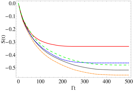
Figure 2: This figure shows the instantaneous thermopower $S(t)$ immediately after the dot level has been moved to its final position for $T_{1}$=0.0035$\Gamma$ (red solid), $T_{2}$=0.0028$\Gamma$ (blue short dashed), $T_{3}$=0.0021$\Gamma$ (orange dot dashed), $T_{4}$=0.0014$\Gamma$ (black dotted), $T_{5}$=0.0007$\Gamma$ (green long dashed) in linear response without any electron-phonon coupling.

We will consider the behaviour of the instantaneous value of the thermopower immediately after the dot level is switched from $\epsilon_{1}=-5\Gamma$ to $\epsilon_{2}=-2\Gamma$ at t=0 via a gate voltage. A transition is triggered from a non-Kondo state to a Kondo state as a result of this abrupt movement. The density of states of the dot both in initial and final levels as well as the parabolic structure of the density of states of the contacts is shown schematically in Fig.1. Since it takes considerable amount of time for the Kondo resonance to form in the final state NordlanderetAl99PRL , dynamical quantities would require a similar amount of time to adjust and reach their steady state values. Consequently, their evolution in the long timescale is non-trivial and requires a careful analysis.

Instantaneous thermopower is displayed for various ambient temperatures in Fig. 2 after switching to the final dot level in infinitesimal bias for zero electron-phonon coupling. In this figure, we clearly observe that the thermopower starts decaying from zero to its steady state value for all temperatures studied. After a certain decay time, it reaches its steady state value. This steady state is negative for all temperature values. However, its absolute value increases until a certain temperature. Once we increase the temperature beyond that, the steady state value starts decreasing but the decay time stays constant. The temperature at which the steady state thermopower reaches its minimum value has been previously identified as the Kondo temperature CostietAl10PRB and our results are in agreement with this observation. The extra insight our results provide is the saturation of the decay time of thermopower and inverse of the saturated decay time. This non-trivial and counter-intuitive result is shown quite strikingly in Fig. 4. We will elaborate on its microscopic nature later on. Both the temperature below which saturation occurs and the inverse of the saturated decay time are equal to the Kondo temperature. These novel observations can become a powerful tool to determine the Kondo temperature during experiments involving thermoelectric switching of a single electron transistor.

Figure 3: This figure shows the instantaneous thermopower $S(t)$ immediately after the dot level has been moved to its final position for $T_{1}$=0.0035$\Gamma$ (red solid), $T_{2}$=0.0028$\Gamma$ (blue short dashed), $T_{3}$=0.0021$\Gamma$ (orange dot dashed), $T_{4}$=0.0014$\Gamma$ (black dotted), $T_{5}$=0.0007$\Gamma$ (green long dashed) in linear response for $g$=2.25.

In Fig. 3, we investigate the instantaneous thermopower for the same parameters used in Fig. 2, but this time we use $g$=2.25 with $\omega_{0}$=0.08$\Gamma$. In this case, the dot level is shifted slightly downwards due to renormalization leading to a smaller Kondo temperature compared to $g$=0 case. As a result, steady state thermopower values are smaller than $g$=0 case if the ambient temperature is above both Kondo temperatures. However, they are larger than $g$=0 case when the ambient temperature is lowered below both Kondo temperatures.

Kondo temperature can once again be identified as the temperature at which steady state thermopower reaches its minimum value. This is also the same temperature below which decay time saturates in analogy with $g$=0 case. The major difference with $g$=0 case lies in the fact that the saturated decay time is now much longer as one can clearly see for the lowest curves in both Fig. 2 and Fig. 3 because the Kondo temperature is much smaller as a result of renormalization of the dot level. In fact, our calculations show that the decay time of thermopower scales with $1/T_{K}$. That is why curves with and without electron-phonon coupling perfectly overlap in Fig. 4. This scaling has been previously observed for time dependent conductance calculations in the absence of any electron-phonon coupling as well PlihaletAl05PRB . Same underlying mechanism holds for thermopower as well because both dynamical quantities depend on the evolution of Kondo resonance whose development has been shown to be inversely proportional to the Kondo temperature NordlanderetAl99PRL .

Figure 4: This figure shows the decay time of thermopower $\tau$ as a function of temperature for both zero and finite electron-phonon coupling strengths. Saturation of the decay time of thermopower around $T_{K}$ is clearly visible here.

Electron-phonon coupling strength $\lambda$ is generally unknown in an experiment. These type of measurements may pave the way for determination of $\lambda$ if the phonon frequency $\omega_{0}$ is known. Once the Kondo temperature is identified via the saturation of decay time described above, Eq. (14) can be solved for renormalized dot level $\overline{\epsilon}$. This would in turn enable to find $\lambda$ because the final bare dot level is adjusted via gate voltage thus known.

It is possible to understand previous numerical results intuitively with the help of Sommerfeld expansion at low temperatures. It is given by

$$S(T)=-\frac{\pi^{2}T}{3A(0,T)}\frac{\partial A}{\partial\epsilon}\rvert_{\epsilon=0}$$ (15)

in atomic units where $A(0,T)$ is the value of the spectral function at Fermi level and $\frac{\partial A}{\partial\epsilon}$ is its derivative. Since the Kondo resonance lies slightly above the Fermi level CostietAl94JPCM , the derivative of the dot density of states at Fermi level is positive. This results in negative thermopower values for all temperatures in Kondo regime due to the negative sign at the beginning of Sommerfeld expansion.

When T$\leq T_{K}$, the Kondo resonance is fully formed in steady state and lowering the temperature any further doesn’t alter its final shape. Similarly, evolution to that final shape takes same amount of time for any $T$ below $T_{K}$. Hence, the decay time of thermopower to its steady state stays constant. However, the steady state value keeps going down in magnitude because of $T$ prefactor in Sommerfeld expansion. This prefactor becomes the only variable below $T_{K}$ in Sommerfeld expansion governing the steady state value since the final shape of spectral function is the same. Subsequently, steady state thermopower curve is nonmonotonic and goes to zero at $T$=0 eventually. This issue has been confirmed by other sources too CostietAl10PRB . On the other hand, the Kondo resonance is simply nonexistent when the dot is in its initial level since T$\gg T_{K}$. Consequently, dot density of states is essentially flat at Fermi level giving rise to zero slope which implies zero thermopower. This is why $S(t)$=0 at $t$=0 and this is in good agreement with previous steady state results CostietAl10PRB .

In conclusion, we investigated the temporal evolution of the thermopower in response to an abrupt movement of the dot level to a position where the Kondo effect is present. We identified both the temperature below which decay time saturates and the inverse of the saturated decay time as new tools to identify the value of the Kondo temperature and the electron-phonon coupling strength. Transient dynamics of thermopower offers a complementary picture to the previous steady state results because providing a detailed analysis of turning this device on and off is crucial for practical device characterization.

In principle, it should be possible to reproduce short time behaviour of our results with time dependent density matrix renormalization group method, however we do not believe it would be sufficient to capture the long timescale governing the development of Kondo resonance since the number of states required to keep the truncation error fixed grows exponentially with time making calculations involving long times unfeasible FeiguinetAl105PRB .

We believe that it is possible to perform this experiment with present day technology because latest advances in ultrafast pump-probe techniques enable to measure the transients down to femtosecond timescale Teradaetal10JPCM ; TeradaetAl10Nature . The entire set-up shown in Fig.1 is kept in a dilution refrigerator in order to access the ambient temperatures around $T_{K}$. This means that both electrodes are in principle at same ambient temperature. One needs to induce a temperature gradient between the contacts in this experiment by irradiating one of the contacts with a laser beam. Consequently, we aim to motivate further experiments in this field with this paper.

AG would like to acknowledge several fruitful discussions with Dr. Xuhui Wang during the initial stages of this project and both authors thank T$\ddot{u}$bitak for generous financial support via grant 111T303.

References

- (1) Committee I R 2004 International Technology Roadmap for Semiconductors (Tokyo: Japan Electronics and Information Technology Industries Association)
- (2) Elzerman J M, Hanson R, van Beveren L H W, Witkamp B, Vandersypen L M K and Kouwenhoven L P 2004 Nature(London) 430 431–434
- (3) Feve G, Mahe A, Berroir J M, Kontos T, Placais B, Glattli D C, Cavanna A, Etienne B and Jin Y 2007 Science 316 1169
- (4) Lu W, Ji Z, Pfeiffer L, West K W and Rimberg A J 2003 Nature 423 422
- (5) Nordlander P, Pustilnik M, Meir Y, Wingreen N S and Langreth D C 1999 Phys. Rev. Lett. 83 808–811
- (6) Plihal M, Langreth D C and Nordlander P 2000 Phys. Rev. B 61 R13341–13344
- (7) Galperin M, Ratner M A and Nitzan A 2007 J. Phys.: Condens. Matter 19 103201
- (8) Merino J and Marston J B 2004 Phys. Rev. B 69 115304
- (9) Plihal M, Langreth D C and Nordlander P 2005 Phys. Rev. B 71 165321
- (10) Izmaylov A F, Goker A, Friedman B A and Nordlander P 2006 J. Phys.: Condens. Matter 18 8995–9006
- (11) Goker A, Friedman B A and Nordlander P 2007 J. Phys.: Condens. Matter 19 376206
- (12) Goker A, Zhu Z Y, Manchon A and Schwingenschlogl U 2010 Phys. Rev. B 82 161304(R)
- (13) Goker A, Zhu Z Y, Manchon A and Schwingenschlogl U 2011 Chem. Phys. Lett. 509 48
- (14) Reddy P, Jang S Y, Segalman R A and Majumdar A 2007 Science 315 1568
- (15) Baheti K, Malen J A, Doak P, Reddy P, Jang S Y, Tilley T D, Majumdar A and Segalman R A 2008 Nano Lett. 8 715
- (16) Malen J A, Doak P, Baheti K, Tilley T D, Majumdar A and Segalman R A 2009 Nano Lett. 9 3406
- (17) Tan A, Sadat S and Reddy P 2010 Appl. Phys. Lett. 96 13110
- (18) Dong B and Lei X L 2002 J. Phys.:Condens. Matter 14 11747
- (19) Costi T A and Zlatic V 2010 Phys. Rev. B 81 235127
- (20) Krawiec M and Wysokinski K I 2006 Phys. Rev. B 73 075307
- (21) Crepieux A, Simkovic F, Cambon B and Michelin F 2011 Phys. Rev. B 83 153417
- (22) Goker A 2011 J. Phys.:Condens. Matter 23 125302
- (23) Werner P and Millis A J 2007 Phys. Rev. Lett. 99 146404
- (24) Shao H X, Langreth D C and Nordlander P 1994 Phys. Rev. B 49 13929–13947
- (25) Feiguin A E, White R S 2005 Phys. Rev. B 72 020404(R)
- (26) Costi T A, Hewson A C and Zlatic V 1994 J. Phys.:Condens. Matter 6 2519
- (27) Terada Y, Yoshida S, Takeuchi O and Shigekawa H 2010 J. Phys.: Condens. Matter 22 264008
- (28) Terada Y, Yoshida S, Takeuchi O and Shigekawa H 2010 Nat. Photon. 4 869