Quaternion Solution for the Rock’n’roller:
Box Orbits, Loop Orbits and Recession

Abstract

We consider two types of trajectories found in a wide range of mechanical systems, viz. box orbits and loop orbits. We elucidate the dynamics of these orbits in the simple context of a perturbed harmonic oscillator in two dimensions. We then examine the small-amplitude motion of a rigid body, the rock’n’roller, a sphere with eccentric distribution of mass. The equations of motion are expressed in quaternionic form and a complete analytical solution is obtained. Both types of orbit, boxes and loops, are found, the particular form depending on the initial conditions. We interpret the motion in terms of epi-elliptic orbits. The phenomenon of recession, or reversal of precession, is associated with box orbits. The small-amplitude solutions for the symmetric case, or Routh sphere, are expressed explicitly in terms of epicycles; there is no recession in this case.

1 Introduction: Box Orbits and Loop Orbits

1.1 Libration and rotation

The simple pendulum, with one degree of freedom, provides a valuable model for a wide range of physical phenomena. The pendulum is constrained to move in a plane, and has two essentially different modes of behaviour. In libration, the bob oscillates about the suspension point, and the angular momentum reverses sign periodically. In rotation the bob moves in a circle with the angular momentum varying periodically but remaining always of one sign. In many systems with more than one degree of freedom there are analogues of these two distinct behaviour patterns. In §2 we investigate this distinction for a perturbed simple harmonic oscillator in two dimensions. In §3 we investigate the dynamics of the rock’n’roller and derive a complete solution for small amplitude motions in terms of quaternions. The dynamics in the case of small asymmetry, $\epsilon=(I_{2}-I_{1})/I_{1}\ll 1$, are examined in §4. The special case of a symmetric body, the Routh Sphere ($\epsilon=0$), is considered in §5 and the solutions are expressed explicitly in terms of epicycles. Concluding remarks are made in §6.

1.2 Stelar motion in a globular cluster

In stellar systems such as triaxial globular clusters, which do not have symmetry about any of the three axes, two distinct types of orbit are found. Since the force is not central, the angular momentum is not conserved. If we consider motions in the symmetry plane perpendicular to one axis, with differing frequencies about the other two directions, we can distinguish two possibilities. In a box orbit, a star oscillates independently about the two axes as it moves along its orbit. As a result of this motion, it fills in a simply connected region of space that includes the centre and that, for small amplitude, approximates a rectangle. The star is free to come arbitrarily close to the centre of the system. If the frequencies with respect to the axes are rationally related, the orbit will be closed. It will then resemble a Lissajous curve. The angular momentum takes both positive and negative values. In a loop orbit, the angular momentum about a perpendicular to the orbital plane remains of one sign. The orbit fills a region limited by two approximately elliptic curves, and is bounded away from the centre. We illustrate the two orbit types in Fig 1, taken from [3, pg. 174].

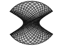
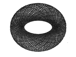
Figure 1: Two orbits in a logarithmic gravitational potential. Left: a box orbit. Right: a loop orbit. Both have equal energy and the character of the orbit is determined by the initial conditions. Figure taken from [3, pg. 174], where further details may be found.

1.3 Motions of the rock’n’roller

The dynamics of a variety of rolling spherical bodies with non-uniform distribution of mass have been studied extensively for more than a century. We refer to such bodies as loaded spheres. We can realize a loaded sphere as a massive triaxial ellipsoid embedded eccentrically in a massless sphere (Fig. 2). The three moments of inertia about the centre of mass are $I_{1}\leq I_{2}\leq I_{3}$, the distance between the centres of mass and symmetry is $a\geq 0$, and the angle between the principal axis corresponding to $I_{3}$ and the line joining the centres of mass and symmetry is denoted $\boldsymbol{\delta}$ (Figure 3). Loaded spheres were investigated by Chaplygin [7], who obtained solutions in a number of particular cases. These bodies have been discussed in several recent publications [6, 9, 10, 14, 15, 16]. Earlier literature is reviewed by [12] and a modern treatment of the dynamics of the loaded sphere is contained in [13].

If the centre of mass and the geometric centre coincide, we call the body the Chaplygin Sphere (CS; See Fig. 3). Chaplygin [8] analysed this case in detail, giving a fairly complete solution. In general, the geometric centre does not lie on an inertial axis. When it does, we call the body the rock’n’roller (RnR). If, in addition, the two moments of inertia transverse to this axis are equal, $I_{1}=I_{2}<I_{3}$, the body is called the Routh Sphere [21]. The case when both these conditions are met — centre of mass at the centre of sphere and $I_{1}=I_{2}$ — has been called Bobylev’s Sphere [4, 10]. Clearly, Bobylev’s Sphere is a special case of both the Routh Sphere and the Chaplygin Sphere. The relationship between the various bodies is shown in Fig. 3.

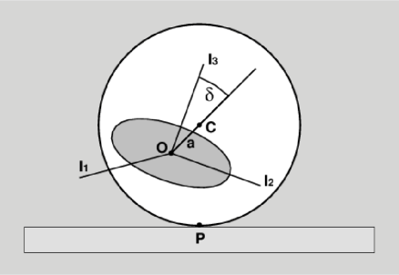
Figure 2: The loaded sphere. In this model, all the mass is contained in the triaxial ellipsoid (shaded), with moments of inertia $I_{1}\leq I_{2}\leq I_{3}$ along the principal axes at the centre of mass $O$. The outer sphere (white) is considered massless. The distance between the centre of mass $O$ and the centre of symmetry $C$ is $a\geq 0$, and the angle between the principal axis corresponding to $I_{3}$ and the line joining the centres of mass and symmetry is denoted $\boldsymbol{\delta}$ (for $a=0$, the angle $\boldsymbol{\delta}$ is undefined). For the rock’n’roller, $\boldsymbol{\delta}=0$.

.

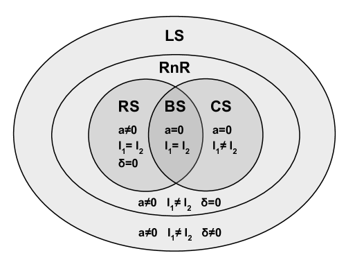
Figure 3: A hierarchy of eccentric spherical bodies. The moments of inertia are $I_{1}\leq I_{2}\leq I_{3}$, the distance between the centres of mass and symmetry is $a\geq 0$, and the angle between the principal axis corresponding to $I_{3}$ and the line joining the centres of mass and symmetry is denoted $\boldsymbol{\delta}$ (for $a=0$, $\boldsymbol{\delta}$ is undefined).
LS: Loaded sphere: $I_{1}<I_{2}<I_{3}$, $a>0$, centre of sphere not on a principal axis ($\boldsymbol{\delta}\neq 0$). RnR: rock’n’roller: $I_{1}<I_{2}<I_{3}$, $a>0$, principal axis through centre of sphere ($\boldsymbol{\delta}=0$). RS: Routh Sphere: $I_{1}=I_{2}<I_{3}$, $a>0$, $\boldsymbol{\delta}=0$. CS: Chaplygin Sphere: $I_{1}<I_{2}<I_{3}$, $a=0$. BS: Bobylev Sphere: $I_{1}=I_{2}<I_{3}$, $a=0$.

.

The dynamics of the rock’n’roller were considered in [19]. The orientation of the body is given by the Euler angles $\phi$, $\theta$, and $\psi$. In the case of the Routh Sphere ($I_{1}=I_{2}<I_{3}$), there are two simple motions: pure rocking in which $\theta$ varies periodically with $\phi$ and $\psi$ constant (mod $\pi$); and pure rolling with $\theta$ constant and $\phi$ and $\psi$ varying steadily. The general motion combines these two modes of oscillation. The azimuthal angle $\phi$ at which the polar angle $\theta$ takes its maximum values increases or decreases regularly and monotonically. This process is called precession. When the symmetry $I_{1}=I_{2}$ is broken, we get the rock’n’roller, and there is a wider range of possible motions. The direction of precession changes intermittently. In [19] we used the term recession to describe this reversal of precession. For a given energy level, recession may or may not occur, depending upon the initial conditions. In Fig. 4 we show the projection of the trajectory of the rock’n’roller onto the $\theta$–$\phi$-plane ($\theta$ radial, $\phi$ azimuthal in plot) for two solutions differing only in their initial conditions. In the left panel, the direction of precession reverses periodically. Clearly, the angular momentum about the vertical takes both positive and negative values. This trajectory has recession, and is an example of a box orbit. In the right panel, the trajectory circulates always in one direction about the centre. While the angular momentum about the vertical is not constant, it is of constant sign. There is no recession; this is an example of a loop orbit.

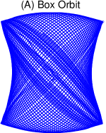
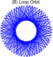
Figure 4: Projection of the trajectory of the rock’n’roller in the $\theta$–$\phi$-plane ($\theta$ radial, $\phi$ azimuthal) with $\epsilon=0.1$ for two solutions differing only in their initial conditions. Panel A: $\theta(0)=\pi/16$, $\phi(0)=\pi/4$, $\psi(0)=\pi/8$ and $\omega_{1}(0)=\omega_{2}(0)=\omega_{3}(0)=0$. Panel B: all parameters as before except $\omega_{3}(0)=0.5$

2 Perturbed Simple Harmonic Oscillator

Many dynamical features of complex physical systems are exhibited clearly in a very simple system, the perturbed simple harmonic oscillator (SHO). The unperturbed system is the two-dimensional SHO with equal frequencies, having the Lagrangian

$$L_{0}=\textstyle\frac{1}{2}(\dot{x}^{2}+\dot{y}^{2})-\textstyle\frac{1}{2}\omega_{0}^{2}(x^{2}+y^{2})=\textstyle\frac{1}{2}(\dot{r}^{2}+r^{2}\dot{\theta}^{2})-\textstyle\frac{1}{2}\omega_{0}^{2}r^{2}\,,$$

where the notation is conventional. The generic solution of this system represents motion in an ellipse centered on the origin. This analytical solution will serve as the basis of a perturbation analysis. The full system that we will study has a Lagrangian

$$L=L_{0}-\delta y^{2}-\epsilon r^{4}\,,$$

where $\delta\ll\omega_{0}^{2}$ and $\epsilon\ll 1$. The $\delta$-term represents a breaking of the $1:1$ resonance of the system $L_{0}$. The $\epsilon$-term represents a radially symmetric stiffening of the restoring force, which results in nonlinear equations of motion.

For $\delta>0$ and $\epsilon=0$, the Hamiltonian is separable:

$$H=H_{x}+H_{y}=\textstyle\frac{1}{2}[\dot{x}^{2}+\omega_{0}^{2}x^{2}]+\textstyle\frac{1}{2}[\dot{y}^{2}+(\omega_{0}^{2}+2\delta)y^{2}]\,,$$

and both components are constant. An analytical solution is immediately found:

$$x = x_{0}\cos\omega_{0}(t-t_{1})$$ (1)

$$y = y_{0}\cos(1+\delta^{\prime})\omega_{0}(t-t_{2})$$ (2)

where $\delta^{\prime}=\sqrt{1+2\delta/\omega_{0}^{2}}-1\approx\delta/\omega_{0}^{2}$. The generic orbit densely fills a rectangular region in the $x$–$y$-plane. If $\delta^{\prime}$ is rational, the orbit is a Lissajous figure and the motion is periodic.

The time evolution of the angular momentum $J=x\dot{y}-y\dot{x}$ is described by

$$\dot{J}=-2\delta xy$$

and clearly $J$ is not conserved, taking both positive and negative values.

For $\delta=0$ and $\epsilon>0$, the restoring force is central and the angular momentum $J$ is conserved. The equation for the radial component is

$$\ddot{r}+\omega_{0}^{2}r+4\epsilon r^{3}-\displaystyle{\frac{2J^{2}}{r^{3}}}=0$$

and an analytical solution for $r$ in terms of elliptic integrals may easily be found. Since the force is central, the angular momentum is conserved. The azimuthal angle $\theta$ follows from integrating the expression for the constant angular momentum, $J=r^{2}\dot{\theta}$.

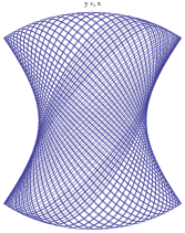
Figure 5: Box and Loop orbits for the perturbed SHO. In both cases, $\lambda=2\epsilon U/\delta=2.236$. All other parameters are equal except the initial position and velocity. Left panel: $x(0)\propto\cos(0.05)$, $y(0)\propto\sin(0.05)$. Right panel: $x(0)\propto\cos(0.5)$, $y(0)\propto\sin(0.5)$.

When both $\delta$ and $\epsilon$ are non-zero, an analytical solution is not so easily found, but numerical integrations produce solutions of both the box orbit and loop orbit types (Fig. 5). To analyse the system, we apply the average Lagrangian technique [23]. The solution is assumed to be of the form

$$x(t)=\Re\{A(t)\exp(i\omega_{0}t)\}\qquad y(t)=\Re\{B(t)\exp(i\omega_{0}t)\}\qquad$$

where the amplitudes $A(t)$ and $B(t)$ are assumed to be slowly varying compared to the exponential terms. Averaging over the period $2\pi/\omega_{0}$ of the fast motion we get

$$\langle L\rangle = \textstyle\frac{1}{4}\Big{[}i\omega_{0}(A\dot{\bar{A}}-\dot{A}{\bar{A}}+B\dot{\bar{B}}-\dot{B}{\bar{B}})-\delta B\bar{B}$$

$$\quad-\epsilon(\textstyle\frac{3}{2}|A|^{4}+2|A|^{2}|B|^{2}+\textstyle\frac{3}{2}|B|^{4}+\Re\{A\bar{B}\}^{2})\Big{]}$$

(overbars denote complex conjugates). Introducing the modulus and phase of $A$ and $B$

$$A=|A|\exp(i\alpha)\qquad B=|B|\exp(i\beta)$$

the average Lagrangian becomes

$$\langle L\rangle = \textstyle\frac{1}{2}\omega_{0}(|A|^{2}\dot{\alpha}+|B|^{2}\dot{\beta})$$

$$-\textstyle\frac{1}{4}\delta|B|^{2}-{\textstyle\frac{1}{8}}\epsilon[3|A|^{4}+4|A|^{2}|B|^{2}+3|B|^{4}+2|A|^{2}|B|^{2}\cos(\alpha-\beta)]$$

We define new coordinates:

$$U=|A|^{2}+|B|^{2}\,,\quad V=|A|^{2}-|B|^{2}\,,\quad\psi=\alpha+\beta\,,\quad\phi=\alpha-\beta$$

Then the Euler-Lagrange equations imply that $U$ is a constant of the motion. It represents to lowest order the value of the total energy

$$E_{0}=\langle\,\textstyle\frac{1}{2}(\dot{x}^{2}+\dot{y}^{2})+\textstyle\frac{1}{2}\omega_{0}^{2}(x^{2}+y^{2})\,\rangle=\textstyle\frac{1}{2}\omega_{0}^{2}U\,.$$

Constancy of $U$ also follows, as the angle $\psi$ is an ignorable coordinate ($\langle L\rangle$ is independent of $\psi$). The equations for $V$ and $\phi$ are

$$\frac{dV}{dt} = \left(\frac{1}{2\omega_{0}}\right)\epsilon(U^{2}-V^{2})\sin 2\phi$$ (3)

$$\frac{d\phi}{dt} = \left(\frac{1}{2\omega_{0}}\right)[\epsilon(1-\cos 2\phi)V-\delta]$$ (4)

We can derive an equation for the average angular momentum,

$$\langle J\rangle=\omega_{0}\Im\{A\bar{B}\}=\textstyle\frac{1}{2}\omega_{0}\sqrt{U^{2}-V^{2}}\sin\phi\,.$$

This shows that $\langle J\rangle$ will change sign if $\phi$ passes through any of the values $n\pi$. We will see that for box orbits $\phi$ is unbounded whereas for loop orbits it is confined to an interval within $(n\pi,(n+1)\pi)$ so that the angular momentum does not change sign.

Defining a new variable $W=V/U$, whose physical range is the interval $[-1,1]$, and re-scaling time by $\tau=(\delta/2\omega_{0})t$, (3) and (4) become

$$\frac{dW}{d\tau} = \lambda(1-W^{2})\sin\phi\cos\phi$$ (5)

$$\frac{d\phi}{d\tau} = \lambda W\sin^{2}\phi-1$$ (6)

where $\lambda=2\epsilon U/\delta$ is a non-dimensional parameter. It is straightforward to show that (5) and (6) are the canonical equations arising from the Hamiltonian

$$h=\textstyle\frac{1}{2}\lambda(1-W^{2})\sin^{2}\phi+W\,.$$

Equations (5) and (6) have equilibrium points when $d\phi/d\tau=dW/d\tau=0$. For $\lambda<1$ there are no such points. For $\lambda>1$ there are equilibrium points at $(\phi,W)=(\pi/2,1/\lambda)$ and $(\phi,W)=(3\pi/2,1/\lambda)$ which are elliptic points or centres. There are also four equilibrium points on the boundary $W=1$, where $\sin^{2}\phi=|1/\lambda|$. These are hyperbolic or saddle points. The phase portraits in the $\phi$–$W$-plane are shown in Fig. 6 (left panel: $\lambda=0.5$; right panel: $\lambda=2.0$).

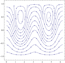
Figure 6: Phase portraits of the perturbed SHO. Left panel: $\lambda=0.5$ (only box orbits exist). Right panel: $\lambda=2.0$ (both box and loop orbits exist). Horizontal axis $\phi$, range $[0,2\pi]$; vertical axis $W$, range $[-1,+1]$.

The two saddle points with $(\sin\phi,W)=(+1/\sqrt{\lambda},1)$ are joined by heteroclinic orbits, as are the two points with $(\sin\phi,W)=(-1/\sqrt{\lambda},1)$. These heteroclinic orbits separate the possible motions into two species. Below (or outside) the separatrices, the variable $\phi$ decreases continually, and the angular momentum $\langle J\rangle=\textstyle\frac{1}{2}\omega_{0}\sqrt{U^{2}-V^{2}}\sin\phi$ changes sign periodically. These trajectories correspond to box orbits. Above (or within) the separatrices, the trajectories surround the centres and the variable $\phi$ is confined to an interval within $(n\pi,(n+1)\pi)$. Thus the angular momentum is of a single sign. Such trajectories correspond to loop orbits.

The value $\lambda=1$ is a bifurcation point for the system (5)–(6). The line $W=1$ corresponds to $B\equiv 0$ and represents an oscillation along the $x$-axis. Likewise, the line $W=-1$ corresponds to $A\equiv 0$ and represents an oscillation along the $y$-axis. For $\lambda<1$ both these motions are stable. For $\lambda>1$ the former is unstable while the latter is stable.

3 Equations of Motion of the rock’n’roller

The rock’n’roller and its symmetric counterpart, the Routh Sphere, were briefly described in §1.3. Here we present the general equations for the motion of the rock’n’roller and also the simplified equations for small amplitude motions.

3.1 Euler angle equations for finite amplitude motion

The equations of motion in terms of Euler angles are given in [19]:

$$\boldsymbol{\Sigma}\mathbf{\dot{\boldsymbol{\theta}}}={\boldsymbol{\omega}}\,,\qquad\bi{K}\mathbf{\dot{\boldsymbol{\omega}}}=\bi{P}_{\boldsymbol{\omega}}$$ (7)

where

$$\mathbf{\dot{\boldsymbol{\theta}}}=\left(\matrix{\dot{\theta}\cr\dot{\phi}\cr\dot{\psi}}\right)\,,\qquad\mathbf{\dot{\boldsymbol{\omega}}}=\left(\matrix{\dot{\omega}_{1}\cr\dot{\omega}_{2}\cr\dot{\omega}_{3}}\right)\,,$$

the matrices $\boldsymbol{\Sigma}$ and $\bi{K}$ are

$$\boldsymbol{\Sigma}=\left[\matrix{\chi&s\sigma&0\cr-\sigma&s\chi&0\cr 0&c&1}\right]\qquad\bi{K}=\left[\matrix{I_{1}+f^{2}+s^{2}\chi^{2}&-s^{2}\sigma\chi&-fs\sigma\cr-s^{2}\sigma\chi&I_{2}+f^{2}+s^{2}\sigma^{2}&-fs\chi\cr-fs\sigma&-fs\chi&I_{3}+s^{2}}\right]$$

and the vector $\bi{P}_{\boldsymbol{\omega}}$ is

$$\bi{P}_{\boldsymbol{\omega}}=\left(\begin{array}[]{l}-(g+\omega_{1}^{2}+\omega_{2}^{2})as\chi+(I_{2}-I_{3}-af)\omega_{2}\omega_{3}\cr\phantom{+}(g+\omega_{1}^{2}+\omega_{2}^{2})as\sigma+(I_{3}-I_{1}+af)\omega_{1}\omega_{3}\cr\phantom{+}(I_{1}-I_{2})\omega_{1}\omega_{2}+as(-\chi\omega_{1}+\sigma\omega_{2})\omega_{3}\end{array}\right)\,,$$

where $s=\sin\theta$, $c=\cos\theta$, $f=c-a$, $\chi=\cos\psi$ and $\sigma=\sin\psi$. Unit mass and radius are assumed and $a$ is the distance from the geometric centre to the centre of mass. Note that neither $\bi{K}$ nor $\bi{\bi{P}_{\boldsymbol{\omega}}}$ depends explicitly on $\phi$. Thus $\phi$ is an ignorable coordinate in the system (7).

To study the fundamental oscillations of the system, we consider motions near the stable equilibrium point $\theta=0$. An attempt to linearize (7) directly, assuming $\theta$ to be small, do not lead to a tractable system: the singularities of $\dot{\phi}$ and $\dot{\psi}$ when $\theta=0$ thwart our endeavours. Thus we are led to seek a system of coordinates that circumvents these singularities and yields simple linear equations for small $\theta$. The unit quaternions provide a suitable system.

3.2 Quaternionic equations for small amplitude motion

The Euler angles relate the orientation of the body frame to that of the space frame. This relationship may also be expressed in terms of Euler’s symmetric parameters, or the Euler-Rodrigues parameters [1, 24], defined by

$$\gamma=\cos\textstyle\frac{1}{2}\theta\cos\textstyle\frac{1}{2}(\phi+\psi)\quad \quad\xi=\sin\textstyle\frac{1}{2}\theta\cos\textstyle\frac{1}{2}(\phi-\psi)$$

$$\zeta=\cos\textstyle\frac{1}{2}\theta\sin\textstyle\frac{1}{2}(\phi+\psi)\quad \quad\eta=\sin\textstyle\frac{1}{2}\theta\sin\textstyle\frac{1}{2}(\phi-\psi)$$

(the notation here differs slightly from [24]; see Appendix A). These parameters satisfy the relationship $\gamma^{2}+\zeta^{2}+\xi^{2}+\eta^{2}=1$. They are the components of a unit quaternion $\mathbf{\mathsf{q}}=\gamma+\xi{\bf i}+\eta{\bf j}+\zeta{\bf k}$.

Expressions for the angular rates of change follow in a straightforward manner:

$$\dot{\theta} = \frac{(\xi\dot{\xi}+\eta\dot{\eta})-(\gamma\dot{\gamma}+\zeta\dot{\zeta})}{\sqrt{(\xi^{2}+\eta^{2})(\gamma^{2}+\zeta^{2})}}$$

$$\dot{\phi} = \left(\frac{\gamma\dot{\zeta}-\zeta\dot{\gamma}}{\gamma^{2}+\zeta^{2}}\right)+\left(\frac{\xi\dot{\eta}-\eta\dot{\xi}}{\xi^{2}+\eta^{2}}\right)$$

$$\dot{\psi} = \left(\frac{\gamma\dot{\zeta}-\zeta\dot{\gamma}}{\gamma^{2}+\zeta^{2}}\right)-\left(\frac{\xi\dot{\eta}-\eta\dot{\xi}}{\xi^{2}+\eta^{2}}\right)$$

Moreover,

$$s =2\sqrt{(\gamma^{2}+\zeta^{2})(\xi^{2}+\eta^{2})}\qquad\qquad c =(\gamma^{2}+\zeta^{2})-(\xi^{2}+\eta^{2})$$

$$\chi =\frac{\gamma\xi+\zeta\eta}{\sqrt{(\gamma^{2}+\zeta^{2})(\xi^{2}+\eta^{2})}}\qquad\qquad\sigma =\frac{\zeta\xi-\gamma\eta}{\sqrt{(\gamma^{2}+\zeta^{2})(\xi^{2}+\eta^{2})}}$$

$$s_{\phi} =\frac{\gamma\eta+\zeta\xi}{\sqrt{(\gamma^{2}+\zeta^{2})(\xi^{2}+\eta^{2})}}\qquad\qquad c_{\phi} =\frac{\gamma\xi-\zeta\eta}{\sqrt{(\gamma^{2}+\zeta^{2})(\xi^{2}+\eta^{2})}}$$

where $s_{\phi}=\sin\phi$ and $c_{\phi}=\cos\phi$. The components of angular velocity are

$$\omega_{1} = 2[\gamma\dot{\xi}-\xi\dot{\gamma}+\zeta\dot{\eta}-\eta\dot{\zeta}]$$

$$\omega_{2} = 2[\gamma\dot{\eta}-\eta\dot{\gamma}+\xi\dot{\zeta}-\zeta\dot{\xi}]$$ (8)

$$\omega_{3} = 2[\gamma\dot{\zeta}-\zeta\dot{\gamma}+\eta\dot{\xi}-\xi\dot{\eta}]$$

At first order in small $\theta$ we may write the Euler-Rodrigues parameters as

$$\gamma=\cos\textstyle\frac{1}{2}(\phi+\psi)=O(1)\quad \quad\xi=\textstyle\frac{1}{2}\theta\cos\textstyle\frac{1}{2}(\phi-\psi)=O(\theta)$$

$$\zeta=\sin\textstyle\frac{1}{2}(\phi+\psi)=O(1)\quad \quad\eta=\textstyle\frac{1}{2}\theta\sin\textstyle\frac{1}{2}(\phi-\psi)=O(\theta)$$

Moreover, at this order of approximation,

$$\omega_{1}=O(\theta)\qquad\omega_{2}=O(\theta)\qquad\omega_{3}=2(\gamma\dot{\zeta}-\zeta\dot{\gamma})=O(1)$$

The third equation of (7) reduces to $\dot{\omega}_{3}=O(\theta^{2})$, so we can take $\omega_{3}$ to be constant. The order-one quaternion elements, $\gamma$ and $\zeta$, are easily found: combining

$$\gamma\dot{\gamma}+\zeta\dot{\zeta}=0\quad\mbox{and}\quad\gamma\dot{\zeta}-\zeta\dot{\gamma}=\textstyle\frac{1}{2}\omega_{3}$$

we see that $\dot{\gamma}=-\textstyle\frac{1}{2}\omega_{3}\zeta$ and $\dot{\zeta}=+\textstyle\frac{1}{2}\omega_{3}\gamma$, which are immediately solved to yield

$$\gamma=\cos\textstyle\frac{1}{2}\omega_{3}(t-t_{00})\,,\qquad\zeta=\sin\textstyle\frac{1}{2}\omega_{3}(t-t_{00})$$ (9)

Here we have used $\gamma^{2}+\zeta^{2}=1$. We choose the time origin such that $t_{00}=0$. The remaining two equations of (7) may now be written

$$\gamma\ddot{\xi}+\zeta\ddot{\eta}-\kappa_{21}\omega_{3}(\zeta\dot{\xi}-\gamma\dot{\eta})+\Omega_{1}^{2}(\gamma\xi+\zeta\eta) = 0$$ (10)

$$\zeta\ddot{\xi}-\gamma\ddot{\eta}+\kappa_{12}\omega_{3}(\gamma\dot{\xi}+\zeta\dot{\eta})+\Omega_{2}^{2}(\zeta\xi-\gamma\eta) = 0$$ (11)

where the constant parameters in the coefficients are

$$\phantom{.}\kappa_{12}=\frac{I_{3}-I_{1}+af_{0}}{I_{2}+f_{0}^{2}} \qquad\phantom{.}\Omega_{10}^{2}=\frac{ga}{I_{1}+f_{0}^{2}} \qquad\phantom{.}\Omega_{1}^{2}=\Omega_{10}^{2}+\textstyle\frac{1}{2}(\kappa_{21}+\textstyle\frac{1}{2})\omega_{3}^{2}$$

$$\phantom{.}\kappa_{21}=\frac{I_{3}-I_{2}+af_{0}}{I_{1}+f_{0}^{2}} \qquad\phantom{.}\Omega_{20}^{2}=\frac{ga}{I_{2}+f_{0}^{2}} \qquad\phantom{.}\Omega_{2}^{2}=\Omega_{20}^{2}+\textstyle\frac{1}{2}(\kappa_{12}+\textstyle\frac{1}{2})\omega_{3}^{2}$$

with $f_{0}=(1-a)$. These equations may be transformed, by a simple rotation, to a system with constant coefficients. We define

$$\left(\matrix{\mu\cr\nu}\right)=\left[\matrix{\gamma&\zeta\cr-\zeta&\gamma}\right]\left(\matrix{\xi\cr\eta}\right)\,.$$ (12)

The following relationships are straightforward to derive:

$$\omega_{1}=2(\dot{\mu}-\omega_{3}\nu)\qquad \dot{\theta}=2(\mu\dot{\mu}+\nu\dot{\nu})/\sqrt{\mu^{2}+\nu^{2}}$$

$$\omega_{2}=2(\dot{\nu}+\omega_{3}\mu)\qquad \dot{\phi}=\omega_{3}+(\mu\dot{\nu}-\nu\dot{\mu})/(\mu^{2}+\nu^{2})$$

$$\omega_{3}=2(\gamma\dot{\zeta}-\zeta\dot{\gamma})\qquad \dot{\psi}=\phantom{\omega_{3}}-(\mu\dot{\nu}-\nu\dot{\mu})/(\mu^{2}+\nu^{2})$$

Equations (10) and (11) may now be written

$$\ddot{\mu}-2k_{2}\dot{\nu}+\tilde{\Omega}_{1}^{2}\mu = 0$$ (13)

$$\ddot{\nu}+2k_{1}\dot{\mu}+\tilde{\Omega}_{2}^{2}\nu = 0$$ (14)

where

$$k_{1} =\textstyle\frac{1}{2}(1-\kappa_{12})\omega_{3}\,,\qquad\tilde{\Omega}_{1}^{2} =\Omega_{10}^{2}+\kappa_{21}\omega_{3}^{2}$$

$$k_{2} =\textstyle\frac{1}{2}(1-\kappa_{21})\omega_{3}\,,\qquad\tilde{\Omega}_{2}^{2} =\Omega_{20}^{2}+\kappa_{12}\omega_{3}^{2}\,.$$

If we seek a solution of (13)–(14) in the form

$$\mu=\mu_{0}\cos\beta(t-t_{0})\qquad\mbox{and}\qquad\nu=\nu_{0}\sin\beta(t-t_{0})$$

the system may be written

$$\left[\matrix{\tilde{\Omega}_{1}^{2}-\beta^{2}&-2k_{2}\beta\cr-2k_{1}\beta&\tilde{\Omega}_{2}^{2}-\beta^{2}}\right]\left(\matrix{\mu_{0}\cr\nu_{0}}\right)=\left(\matrix{0\cr 0}\right)$$ (15)

The determinant is a biquadratic in $\beta$ with four real roots, occurring in positive and negative pairs. We denote the positive eigenvalues by $\beta_{1}$ and $\beta_{2}$ and assume that $0\leq\beta_{1}\leq\beta_{2}$. The eigenvectors are $(1,\lambda_{1})^{\rm T}$ and $(1,\lambda_{2})^{\rm T}$, with

$$\lambda_{1}=\frac{\tilde{\Omega}_{1}^{2}-\beta_{1}^{2}}{2k_{2}\beta_{1}}=\frac{2k_{1}\beta_{1}}{\tilde{\Omega}_{2}^{2}-\beta_{1}^{2}}\,,\qquad\lambda_{2}=\frac{\tilde{\Omega}_{1}^{2}-\beta_{2}^{2}}{2k_{2}\beta_{2}}=\frac{2k_{1}\beta_{2}}{\tilde{\Omega}_{2}^{2}-\beta_{2}^{2}}$$ (16)

and we can write the general solution of (13)–(14) as

$$\mu =\phantom{\lambda_{1}}\mu_{1}\cos\beta_{1}(t-t_{1}) +\phantom{\lambda_{2}}\mu_{2}\cos\beta_{2}(t-t_{2})$$ (17)

$$\nu =\lambda_{1}\mu_{1}\sin\beta_{1}(t-t_{1}) +\lambda_{2}\mu_{2}\sin\beta_{2}(t-t_{2})$$ (18)

The equations (13)–(14) are now completely solved. The solution (17)–(18) is determined by the initial conditions $\{\mu_{1},\mu_{2},t_{1},t_{2}\}$. These are equivalent to conditions $\{\mu(0),\dot{\mu}(0),\nu(0),\dot{\nu}(0)\}$. Solutions of (10)–(11) follow immediately by means of (9) and (12).

3.3 Lagrangian and Hamiltonian

Equations (13)–(14) may be derived from the Lagrangian

$$L=\textstyle\frac{1}{2}(k_{1}\dot{\mu}^{2}+k_{2}\dot{\nu}^{2})-\textstyle\frac{1}{2}(k_{1}\tilde{\Omega}_{1}^{2}\mu^{2}+k_{2}\tilde{\Omega}_{2}^{2}\nu^{2})+k_{1}k_{2}(\mu\dot{\nu}-\nu\dot{\mu})$$

The generalized momenta are $p_{\mu}=k_{1}(\dot{\mu}-k_{2}\nu)$ and $p_{\nu}=k_{2}(\dot{\nu}+k_{2}\mu)$ and the Hamiltonian, obtained from the Legendre transformation, is

$$H=\textstyle\frac{1}{2}\displaystyle{\left(\frac{p_{\mu}^{2}}{k_{1}}+\frac{p_{\nu}^{2}}{k_{2}}\right)} - [k_{1}\mu p_{\nu}-k_{2}\nu p_{\mu}]$$

$$+ \textstyle\frac{1}{2}[k_{1}(k_{1}k_{2}+\tilde{\Omega}_{1}^{2})\mu^{2}+k_{2}(k_{1}k_{2}+\tilde{\Omega}_{2}^{2})\nu^{2}]$$

The numerical value of the Hamiltonian is equal to the (constant) energy

$$E_{\mu+\nu}=\textstyle\frac{1}{2}(k_{1}\dot{\mu}^{2}+k_{2}\dot{\nu}^{2})+\textstyle\frac{1}{2}(k_{1}\tilde{\Omega}_{1}^{2}\mu^{2}+k_{2}\tilde{\Omega}_{2}^{2}\nu^{2})$$

An additional constant of the motion can be found from the solutions (17)–(18) for $\mu$ and $\nu$ and their time derivatives for $\dot{\mu}$ and $\dot{\nu}$. We can solve the four expressions for the sines and cosines in terms of $\{\mu,\nu,\dot{\mu},\dot{\nu}\}$. These can then be combined to yield the following constants:

$$K_{1} \equiv\left(\frac{\lambda_{2}\dot{\mu}+\beta_{2}\nu}{\beta_{1}\lambda_{2}-\beta_{2}\lambda_{1}}\right)^{2}+\left(\frac{\dot{\nu}-\beta_{2}\lambda_{2}\mu}{\beta_{1}\lambda_{1}-\beta_{2}\lambda_{2}}\right)^{2} =\mu_{1}^{2}\,,$$ (20)

$$K_{2} \equiv\left(\frac{\lambda_{1}\dot{\mu}+\beta_{1}\nu}{\beta_{1}\lambda_{2}-\beta_{2}\lambda_{1}}\right)^{2}+\left(\frac{\dot{\nu}-\beta_{1}\lambda_{1}\mu}{\beta_{1}\lambda_{1}-\beta_{2}\lambda_{2}}\right)^{2} =\mu_{2}^{2}\,.$$ (21)

Numerical tests confirm that $K_{1}$ and $K_{2}$ remain constant. They may be combined linearly to form $E_{\mu+\nu}$ and an additional independent constant.

4 Epi-elliptic solution for small asymmetry $\mathbf{(\epsilon=(I_{2}-I_{1})/I_{1}\ll 1)}$

For the symmetric case, $\epsilon=0$ and the matrix in (15) takes the simple form

$$\left[\matrix{A&-B\cr-B&A}\right]$$

so that the eigenvectors are multiples of $(1,1)^{\rm T}$ and $(1,-1)^{\rm T}$. For $\epsilon\neq 0$, this is no longer the case. The eigenvalues are perturbed to $\beta_{1}=\beta_{1}^{0}+\delta\beta_{1}$ and $\beta_{2}=\beta_{2}^{0}+\delta\beta_{2}$, where $\beta_{1}^{0}$ and $\beta_{2}^{0}$ are the values for $\epsilon=0$. The eigenvectors are $(1,\lambda_{1})^{\rm T}$ and $(1,\lambda_{2})^{\rm T}$ and, for small asymmetry ($\epsilon\ll 1$), we have $\lambda_{1}\approx+1$ and $\lambda_{2}\approx-1$.

The complete solution of the rock’n’roller equations for small amplitude motion is

$$\gamma =\cos\textstyle\frac{1}{2}\omega_{3}t$$ (22)

$$\zeta =\sin\textstyle\frac{1}{2}\omega_{3}t$$ (23)

$$\mu =\phantom{\lambda_{1}}\mu_{1}\cos\beta_{1}(t-t_{1}) +\phantom{\lambda_{2}}\mu_{2}\cos\beta_{2}(t-t_{2})$$ (24)

$$\nu =\lambda_{1}\mu_{1}\sin\beta_{1}(t-t_{1}) +\lambda_{2}\mu_{2}\sin\beta_{2}(t-t_{2})$$ (25)

The projection in the $\gamma$–$\zeta$-plane, given by (22)–(23), is a rotation with frequency $\textstyle\frac{1}{2}\omega_{3}$. The solution (24)–(25) has two components, each having a trajectory that is elliptic (for the Routh Sphere, $\epsilon=0$, they are both circular). The first component is

$$\mu=\mu_{1}\cos[\beta_{1}(t-t_{1})]\,,\qquad\nu=\mu_{1}\lambda_{1}\sin[\beta_{1}(t-t_{1})]\,,$$

elliptical motion with frequency $\beta_{1}$ and semi-axes $\mu_{1}$ and $\mu_{1}\lambda_{1}$, counterclockwise if $\lambda_{1}>0$ (recall that $\lambda_{1}=1$ in the limiting case $\epsilon=0$). The second component is

$$\mu=\mu_{2}\cos[\beta_{2}(t-t_{2})]\,,\qquad\nu=\mu_{2}\lambda_{2}\sin[\beta_{2}(t-t_{2})]\,,$$

elliptical motion with frequency $\beta_{2}$ and semi-axes $\mu_{2}$ and $\mu_{2}\lambda_{2}$, clockwise if $\lambda_{2}<0$ (and $\lambda_{2}=-1$ in the limiting case $\epsilon=0$). The overall character of the trajectory is thus determined by the relative magnitudes and signs of the parameters $\{\lambda_{1},\lambda_{2}\}$ and the initial conditions $\{\mu_{1},\mu_{2}\}$.

In Fig 7 we illustrate two characteristic solutions in the $\mu$–$\nu$-plane. In both cases, $\beta_{1}=1/\pi$ and $\beta_{2}=1$. In the left panel, $\mu_{2}<\mu_{1}$ and also $\mu_{2}\lambda_{2}<\mu_{1}\lambda_{1}$, the orbit circulates about the centre, sometimes curving towards it and sometimes curving away. We call this a centrifugal orbit. The representative point is bounded away from the centre. For the solution in the right panel, $\mu_{2}>\mu_{1}$ and also $\mu_{2}\lambda_{2}>\mu_{1}\lambda_{1}$. The orbit circulates about the centre, $\mu=\nu=0$, always curving towards it. We call this a centripetal orbit.

It is clear on geometric grounds that if $(|\mu_{1}|-|\mu_{2}|)$ and $(|\lambda_{1}\mu_{1}|-|\lambda_{2}\mu_{2}|)$ are of the same sign, the trajectory cannot reach the centre, $\mu=\nu=0$. Thus, the criterion for recession may be written

$$(|\mu_{1}|-|\mu_{2}|)\cdot(|\lambda_{1}\mu_{1}|-|\lambda_{2}\mu_{2}|)<0$$ (26)

(see Appendix B). In this case, the orbit may approach arbitrarily close to the centre, and the angular momentum about the centre may change sign.

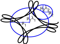
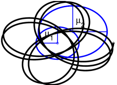
Figure 7: Rock’n’roller: the trajectories in the $\mu$–$\nu$-plane are epi-ellipses. Left: $\mu_{1}=1$, $\mu_{2}=0.5$, $\lambda_{1}=0.75$, $\lambda_{2}=-0.75$. Right: $\mu_{1}=1$, $\mu_{2}=1.6$, $\lambda_{1}=0.75$, $\lambda_{2}=-0.75$. In both cases, $\beta_{1}=1$ and $\beta_{2}=1/\pi$.

4.1 Special case: central orbits with $\omega_{3}=0$

The case $\omega_{3}=0$ is especially simple: $(\mu,\nu)=(\xi,\eta)\approx(\textstyle\frac{1}{2}\theta\cos\phi,\textstyle\frac{1}{2}\theta\sin\phi)$, so the trajectories in the $\mu$–$\nu$-plane are structurally identical to those on a polar $\theta$–$\phi$ plot (with $\theta$ radial and $\phi$ azimuthal). Equations (13)–(14) take a particularly simple form

$$\ddot{\mu}+\Omega_{10}^{2}\mu\qquad\mbox{\rm and}\qquad\ddot{\nu}+\Omega_{20}^{2}\nu$$

and the solution may be written immediately:

$$\mu = \mu_{0}\cos\Omega_{10}(t-t_{1})$$ (27)

$$\nu = \nu_{0}\sin\Omega_{20}(t-t_{2})$$ (28)

which is mathematically equivalent to the solution (1)–(2) of the simple harmonic oscillator. Clearly, $\mu_{0}\neq 0$ and $\nu_{0}=0$ yields pure rocking motion in one principal direction, while $\mu_{0}=0$ and $\nu_{0}\neq 0$ yields pure rocking in another. The case of a central orbit, $\mu_{0}=\nu_{0}$ is of particular interest. The angular momentum quantity $K=(\mu\dot{\nu}-\nu\dot{\mu})+k(\mu^{2}+\nu^{2})$ (which we shall see to be constant when $\epsilon=0$) is easily shown to have two components

$$K=\mu_{0}^{2}\bar{\Omega}\cos(2\Omega^{\prime}t-\rho)+\mu_{0}^{2}\Omega^{\prime}\cos(2\bar{\Omega}t-\sigma)$$

where $\bar{\Omega}=\textstyle\frac{1}{2}(\Omega_{10}+\Omega_{20})$ and $\Omega^{\prime}=\textstyle\frac{1}{2}(\Omega_{10}-\Omega_{20})$. The first component is of large amplitude and low frequency, the second is of small amplitude and high frequency. Generically, the trajectory of the solution densely fills a square region in the $\mu$–$\nu$-plane.

5 The Routh Sphere $\mathbf{(I_{1}=I_{2})}$: complete solution for small amplitude

Let us now consider the solution for the Routh Sphere, the symmetric case with $I_{1}=I_{2}$ or $\epsilon=0$, so that $\kappa_{12}=\kappa_{21}=\kappa$, $k_{1}=k_{2}=k$ and $\tilde{\Omega}_{1}^{2}=\tilde{\Omega}_{2}^{2}=\tilde{\Omega}^{2}$. Then the (positive) eigenvalues for the system (15) are

$$\beta_{1,2}=\mp k+\sqrt{k^{2}+\tilde{\Omega}^{2}}$$

where $k=\textstyle\frac{1}{2}(1-\kappa)\omega_{3}$, and the eigenvectors are $(1,1)^{\rm T}$ and $(1,-1)^{\rm T}$. The general solution is

$$\mu = \mu_{1}\cos\beta_{1}(t-t_{1})+\mu_{2}\cos\beta_{2}(t-t_{2})$$ (29)

$$\nu = \mu_{1}\sin\beta_{1}(t-t_{1})-\mu_{2}\sin\beta_{2}(t-t_{2})$$ (30)

It follows immediately that

$$\mu^{2}+\nu^{2} = \mu_{1}^{2}+\mu_{2}^{2}+2\mu_{1}\mu_{2}\cos[(\beta_{1}+\beta_{2})t-b_{12}]$$ (31)

$$\mu\dot{\nu}-\nu\dot{\mu} = \mu_{1}^{2}\beta_{1}-\mu_{2}^{2}\beta_{2}+\mu_{1}\mu_{2}(\beta_{1}-\beta_{2})\cos[(\beta_{1}+\beta_{2})t-b_{12}]$$

$$\mu\dot{\mu}+\nu\dot{\nu} = -\mu_{1}\mu_{2}(\beta_{1}+\beta_{2})\sin[(\beta_{1}+\beta_{2})t-b_{12}]$$

where $b_{12}=\beta_{1}t_{1}+\beta_{2}t_{2}$ is a fixed phase. When the third of these quantities, namely $\mu\dot{\mu}+\nu\dot{\nu}$, vanishes, $\dot{\theta}=0$ and $\theta$ reaches an extremum. This occurs when

$$(\beta_{1}+\beta_{2})t-b_{12}=n\pi\qquad\mbox{or}\qquad t=t_{n}^{0}\equiv\frac{n\pi+b_{12}}{\beta_{1}+\beta_{2}}$$

The cosine factors then take the value $(-1)^{n}$. We find that

$$\dot{\phi}_{2n}=\omega_{3}+\frac{\mu_{1}\beta_{1}-\mu_{2}\beta_{2}}{\mu_{1}+\mu_{2}}\qquad\dot{\phi}_{2n+1}=\omega_{3}+\frac{\mu_{1}\beta_{1}+\mu_{2}\beta_{2}}{\mu_{1}-\mu_{2}}$$

Note that both $\dot{\phi}_{2n}$ and $\dot{\phi}_{2n+1}$ are independent of $n$. If they are of the same sign, the azimuthal angle $\phi$ changes monotonically with time. If not, the body executes a reverse loop in each cycle. However, there is no recession in either case; this would require $\dot{\phi}_{n}$ to be a function of $n$.

The absence of recession also follows immediately from (31). This implies that the distance from the origin of the $\mu$–$\nu$-plane varies between $\big{|}|\mu_{1}|-|\mu_{2}|\big{|}$ and $|\mu_{1}|+|\mu_{2}|$. So, unless $|\mu_{1}|=|\mu_{2}|$, the accessible region is annular, and the angular momentum about $\mu=\nu=0$ cannot change sign.

It is straightforward to show that the equations of the Routh Sphere have two constants, the energy quantity

$$E_{\mu+\nu}=\textstyle\frac{1}{2}(\dot{\mu}^{2}+\dot{\nu}^{2})+\textstyle\frac{1}{2}\tilde{\Omega}^{2}(\mu^{2}+\nu^{2})$$

and a quantity relating to angular momentum,

$$K=(\mu\dot{\nu}-\nu\dot{\mu})+k(\mu^{2}+\nu^{2})$$

This quantity may be written in terms of the initial conditions

$$K=\sqrt{k^{2}+\tilde{\Omega}^{2}}(\mu_{1}^{2}-\mu_{2}^{2})$$ (32)

This is interesting, as it allows us to characterise the solution in terms of the relative sizes of $\mu_{1}$ and $\mu_{2}$.

We recall from [19] that the Routh Sphere has two constants in addition to the energy, Jellett’s constant and Routh’s constant:

$$Q_{J}=I_{1}s^{2}\dot{\phi}+I_{3}f\omega_{3}\qquad\mbox{and}\qquad Q_{R}=\omega_{3}/\rho$$

where the density $\rho$ is defined by $\rho=1/\sqrt{I_{3}+s^{2}+(I_{3}/I_{1})f^{2}}$. To $O(\theta^{2})$, these may be written

$$\tilde{Q}_{J} = (I_{1}\theta^{2}\dot{\phi}+I_{3}f_{0}\omega_{3})-\textstyle\frac{1}{2}I_{3}\omega_{3}\theta^{2}$$

$$\tilde{Q}_{R} = \left[1+\left(\frac{I_{1}-I_{3}f_{0}}{(I_{1}+f_{0}^{2})I_{3}}\right)\frac{\theta^{2}}{2}\right]\frac{\omega_{3}}{\rho_{0}}$$

where $\rho_{0}=1/\sqrt{(I_{1}+f_{0}^{2})I_{3}/I_{1}}$. We can now show that

$$K=\frac{1}{4I_{1}}\left[\tilde{Q}_{J}-I_{3}f_{0}\rho_{0}\tilde{Q}_{R}\right]$$ (33)

This allows us to relate the solution in terms of $\mu_{1}$ and $\mu_{2}$ (or $K$), to the quantities $\tilde{Q}_{J}$ and $\tilde{Q}_{R}$ (cf. Fig. 4 in [19]).

5.1 Epicycle character of the solution

We will first interpret the solution in the $\mu$–$\nu$-plane, noting that it bears a correspondence to the $\theta$–$\phi$-plane through the relationships

$$\theta=2\sqrt{\mu^{2}+\nu^{2}}\,,\qquad\phi=\omega_{3}t+\arctan{(\nu/\mu)}$$

We note that the solution (29)–(30) is comprised of two components: the first

$$\mu=\mu_{1}\cos[\beta_{1}(t-t_{1})]\,,\qquad\nu=\mu_{1}\sin[\beta_{1}(t-t_{1})]$$

is a counterclockwise circular motion with frequency $\beta_{1}$ and radius $\mu_{1}$; the second

$$\mu=\mu_{2}\cos[\beta_{2}(t-t_{2})]\,,\qquad\nu=-\mu_{2}\sin[\beta_{2}(t-t_{2})]$$

is a clockwise circular motion with frequency $\beta_{2}$ and radius $\mu_{2}$. The complete motion is thus an epicycle.

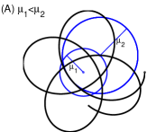
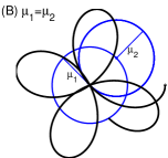
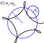
Figure 8: Routh Sphere: the trajectories in the $\mu$–$\nu$-plane are epicycles. The three distinct cases are illustrated: left panel $\mu_{1}<\mu_{2}$ (centripetal orbit in $\mu$–$\nu$-plane); centre panel $\mu_{1}=\mu_{2}$ (central orbit); right panel $\mu_{1}>\mu_{2}$ (centrifugal orbit in $\mu$–$\nu$-plane). The frequencies are $\beta_{1}=0.3$ (counterclockwise) and $\beta_{2}=1.0$ (clockwise).

We illustrate various possibilities schematically in Fig. 8. For $\mu_{1}<\mu_{2}$, the orbit circulates about the centre, $\mu=\nu=0$, always curving towards it in a centripetal orbit (Fig. 8(A)). For $\mu_{1}>\mu_{2}$, the orbit circulates in the opposite direction about the centre, sometimes curving towards it and sometimes curving away. This is a centrifugal orbit (Fig. 8(C)). For $\mu_{1}=\mu_{2}$, the orbit passes periodically through the centre $\mu=\nu=0$. We call this a central orbit (Fig. 8(B)); for further discussion, see Appendix B.

We have chosen $0\leq\beta_{1}\leq\beta_{2}$ by arbitrary convention. The solution for $\mu$ and $\nu$ is given by (29)–(30). To transform back to the $\theta$–$\phi$-plane, we must rotate through an angle $\omega_{3}t$. Defining $x=(\theta/2)\cos\phi,y=(\theta/2)\sin\phi$, we have

$$x = \mu_{1}\cos(\alpha_{1}t-\beta_{1}t_{1})+\mu_{2}\cos(\alpha_{2}t-\beta_{2}t_{1})$$

$$y = \mu_{1}\sin(\alpha_{1}t-\beta_{1}t_{1})-\mu_{2}\sin(\alpha_{2}t-\beta_{2}t_{1})$$

where the frequencies are $\alpha_{1}=\beta_{1}+\omega_{3}$ and $\alpha_{2}=\beta_{2}-\omega_{3}$. We find that $0\leq\alpha_{2}\leq\alpha_{1}$. This effectively switches the roles of the two components of the solution: centripetal motion in the $\mu$–$\nu$-plane corresponds to centrifugal in the $\theta$–$\phi$-plane, and vice versa. Referring to (32) and (33), we see that the following correspondence holds:

$${\ }[\mu_{1}>\mu_{2}]\Longleftrightarrow[K>0] \Longleftrightarrow [\tilde{Q}_{J}>\tilde{Q}_{J,0}^{\rm crit}]\Longleftrightarrow[\mbox{\rm Centripetal (in}\ \theta\mbox{--}\phi\mbox{-plane})]$$

$${\ }[\mu_{1}=\mu_{2}]\Longleftrightarrow[K=0] \Longleftrightarrow [\tilde{Q}_{J}=\tilde{Q}_{J,0}^{\rm crit}]\Longleftrightarrow[\mbox{\rm Central (in}\ \theta\mbox{--}\phi\mbox{-plane})]$$

$${\ }[\mu_{1}<\mu_{2}]\Longleftrightarrow[K<0] \Longleftrightarrow [\tilde{Q}_{J}<\tilde{Q}_{J,0}^{\rm crit}]\Longleftrightarrow[\mbox{\rm Centrifugal (in}\ \theta\mbox{--}\phi\mbox{-plane})]$$

where $\tilde{Q}_{J,0}^{\rm crit}=I_{3}f_{0}\rho_{0}\tilde{Q}_{R}$ (see also Fig. 4 in [19]).

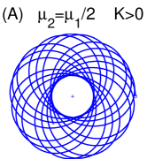
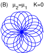
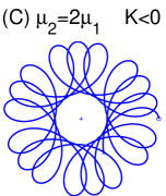
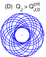
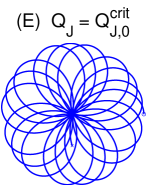
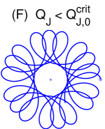
Figure 9: Routh Sphere: the trajectories in the $\theta$–$\phi$-plane are epicycles. Panels (A)–(C): Analytical solutions of the quaternion equations for three sets of initial conditions: (A) $\mu_{2}=0.5\mu_{1}$; (B) $\mu_{2}=\mu_{1}$; (C) $\mu_{2}=2\mu_{1}$. In all cases, $\mu_{1}=1$ and $t_{1}=t_{2}=0$. Panels (D)–(F): Numerical solutions of the full nonlinear equations for the corresponding initial conditions: (D) $\omega_{2}(0)=0.008147$; (E) $\omega_{2}(0)=0.005389$; (F) $\omega_{2}(0)=0.002632$. In all cases $\theta(0)=0.01$, $\omega_{3}(0)=1.0$ and $\phi(0)=\psi(0)=\omega_{1}(0)=0$.

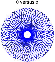
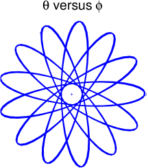
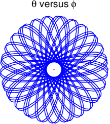
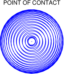
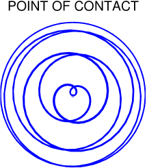
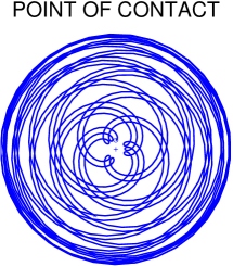
Figure 10: Top row: trajectories in the $\theta$–$\phi$-plane for three sets of initial conditions, $\omega_{2}=0.001005$, $\omega_{3}(0)=0.02$ (left), $\omega_{2}=0.001384$, $\omega_{3}(0)=0.09$ (centre) and $\omega_{2}=0.001658$, $\omega_{3}(0)=0.14$ (right). Bottom row: corresponding plots of the trajectory of the point of contact. In all cases $\theta(0)=0.01$, $\phi(0)=0$, $\psi(0)=0$ and $\omega_{1}(0)=0$ and $\mu_{2}/\mu_{1}=\frac{3}{4}$. The solutions in the central column satisfy the criterion (36).

5.2 Trajectory of the point of contact

So far, we have looked at the projections of the orbit in the $\mu$–$\nu$-plane and in the $\theta$–$\phi$-plane. However, the external observer is aware of both the orientation of the body, as determined by the Euler angles and the position as given by the coordinates $(X,Y)$ of the geometric centre or, equivalently, the point of contact.

The movement of the geometric centre is linked to the angular velocity of the body through the rolling constraint [19]:

$$(\dot{X},\dot{Y},0)=\mathbf{\boldsymbol{\omega}\boldsymbol{\times}K}$$

where $\mathbf{K}$ is a unit vertical vector. In terms of quaternions, this becomes

$$\dot{X} = 2[\gamma\dot{\eta}-\eta\dot{\gamma}+\zeta\dot{\xi}-\xi\dot{\zeta}]$$

$$\dot{Y} = 2[\xi\dot{\gamma}-\gamma\dot{\xi}+\zeta\dot{\eta}-\eta\dot{\zeta}]$$

Substituting the solutions (9), (17) and (18) for the quaternion components, we get

$$X = \phantom{-.}\left[{2\mu_{1}\beta_{1}}/{\alpha_{1}}\right]\sin(\alpha_{1}t-\beta_{1}t_{1})-\left[{2\mu_{2}\beta_{2}}/{\alpha_{2}}\right]\sin(\alpha_{2}t-\beta_{2}t_{2})$$ (34)

$$Y = -\left[{2\mu_{1}\beta_{1}}/{\alpha_{1}}\right]\cos(\alpha_{1}t-\beta_{1}t_{1})-\left[{2\mu_{2}\beta_{2}}/{\alpha_{2}}\right]\cos(\alpha_{2}t-\beta_{2}t_{2})$$ (35)

We saw that the criterion for a central orbit, or the boundary between a centripetal and a centrifugal orbit, in the $\theta$–$\phi$-plane was $\mu_{1}=\mu_{2}$. The corresponding boundary for the $X$–$Y$-plane is the equality of the coefficients in (34)–(35) or

$$\frac{\mu_{1}\beta_{1}}{\alpha_{1}}=\frac{\mu_{2}\beta_{2}}{\alpha_{2}}$$ (36)

The distinction is a reflection of the nonholonomic nature of the constraint: we cannot express $(X,Y)$ in terms of the Euler angles until the solution is found.

In Fig. 10 we show trajectories in the $\theta$–$\phi$-plane (top row) and corresponding plots for the point of contact (bottom row). In the three cases, the orbit is centripetal in the $\theta$–$\phi$-plane but in the $X$–$Y$-plane it changes character, from centripetal to central to centrifugal as $\omega_{3}$ increases. The solutions in the central column of Fig. 10 satisfy the criterion (36).

6 Conclusion

Box and loop orbits are found in a wide range of physical systems. We illustrate them in the elementary context of a perturbed simple harmonic oscillator. Then, the dynamical equations for small amplitude motions of the rock’n’roller are expressed in terms of quaternions. The complete solution is expressed as an epi-ellipse, a combination of two purely elliptic motions. This allows us to clarify the phenomenon of recession, and the conditions under which it occurs. In the particular case of a symmetric body ($\epsilon=0$), the Routh Sphere, the solution reduces to an epicycle. Only loop orbits occur and there is no recession.

We have confined attention in the present study to the dynamics at first order in the polar angle $\theta$. In an extension of this work, we will present a more detailed perturbation analysis, including a rigorous demonstration of energy conservation to second order, explicit expressions for the Routh and Jellett quantities $Q_{R}$ and $Q_{J}$ and a complete analysis of the recession of the rock’n’roller.

The dynamics of the rattleback or celt have been discussed in many publications; see, for example, [5]. It is an ellipsoidal body that exhibits a variety of reversals of rotation. While the dominant behaviour of the rattleback is due to the mis-allignment of its inertial and geometric axes, the mechanism of recession described here for the rock’n’roller must also be present, and may be proposed as a mechanism accounting for observed multiple reversals of the rattleback. This speculation deserves further consideration.

One of the motivations for studying the rock’n’roller is the hope of finding an invariant of the motion in addition to the energy. This expectation arises from the symmetry of the body. For the general loaded sphere, there is a finite angle $\boldsymbol{\delta}$ between the principal axis corresponding to $I_{3}$ and the line joining the centres of gravity and symmetry. For the rock’n’roller, this angle is zero and the Lagrangian is independent of the azimuthal angle $\phi$. However, we have not found a second invariant and, considering the non-holonomic nature of the problem, its existence remains an open question.

Appendix A: Euler Angle Ambiguity

In his work on celestial mechanics, Euler showed that any two independent orthogonal frames can be related by (not more than) three rotations about the coordinate axes. Kuipers [17] lists twelve sequences of rotations. The first, denoted $xyz$, means a rotation about the $x$-axis, followed by a rotation about the new $y$-axis followed by a rotation about the newer $z$-axis. Different choices are made in different areas of science, frequently leading to ambiguity in the meaning of the Euler angles. In mechanics, two sequences are in common use, each commanding the respect due to its adoption by renowned authorities.

We denote the unit orthogonal triad in the space frame by $(\mathbf{I,J,K})$ and the corresponding triad in the body frame by $(\mathbf{i,j,k})$. Coordinates in the space frame are $(X,Y,Z)$ and in the body frame $(x,y,z)$. The origin is colocated in the two frames. The body frame may be related to the space frame by a set of three rotations. In both rotation sequences, the first rotation is about the (space) $Z$ axis (about the vector $\mathbf{K}$), and the third is about the (body) $z$ axis (about the vector $\mathbf{k}$). However, the axis of the second rotation differs in the two sequences and, as a result, the magnitudes of the rotations also differ.

The first sequence is the $zxz$-sequence, and we denote the Euler angles in this case by $(\phi,\theta,\psi)$. In this $zxz$-sequence, favoured by Landau & Lifshitz [18], Arnold [2] and Goldstein et al. [11], the second rotation is of an angle $\theta$ about the $x$-axis that results from the first rotation. In the second sequence, $zyz$, employed by Whittaker [24] and by Synge and Griffith [22], we denote the angles by $(\Phi,\Theta,\Psi)$. The second rotation is now through an angle $\Theta$ about the $y$-axis that results from the first rotation. The overall rotation must be identical for the two sequences. Constructing the rotation matrix for the composition of the three rotations in each case and equating the two results, we find that the relationship between the Euler anges in the two sequences is

$$\Phi=\phi-\frac{\pi}{2}\qquad\Theta=\theta\qquad\Psi=\psi+\frac{\pi}{2}\,.$$

These relationships enable us to convert between the two conventions. The full rotation matrix for $zxz$ is given, for example, in Goldstein et al. [11, pg. 153], and in Marsden and Ratiu [20, pg. 494]. For the $zyz$ sequence, the rotation matrix is given in Whittaker [24, pg. 10] and in Synge and Griffith [22, pg. 261].

The quaternion representing the rotation must be independent of the Euler angle convention. However, the expressions for the quaternion components in terms of the angles will be different in each case. This explains why our definitions of the components $(\gamma,\xi,\eta,\zeta)$ are different from those of $(\chi,\xi,\eta,\zeta)$ in Whittaker [24]. The expansion of the components of angular velocity $(\omega_{1},\omega_{2},\omega_{3})$ in terms of angles is also different in the two conventions, but their expression in terms of $(\gamma,\xi,\eta,\zeta)$ is identical. Thus, many of the formulae we derive are the same as those found in [24], except that we replace $\chi$ by $\gamma$ to avoid confusion with our notation for $\cos\psi$.

Altmann [1] observes that sequence $zyz$ is now universal in quantum physics, as it is consistent with the Condon and Shortley convention. In the context of classical mechanics, there is no obvious advantage of either convention over the other. However, we feel that it is important to avoid any ambiguity by making the choice clear. Sequence $zxz$ is used in the present paper.

Appendix B: Epicyclic and epi-elliptic orbits

Epicyclic motion

We consider the character of solutions of the form

$$\mu =\phantom{\lambda_{1}}\mu_{1}\cos\beta_{1}(t-t_{1}) +\phantom{\lambda_{2}}\mu_{2}\cos\beta_{2}(t-t_{2})$$ (37)

$$\nu =\lambda_{1}\mu_{1}\sin\beta_{1}(t-t_{1}) +\lambda_{2}\mu_{2}\sin\beta_{2}(t-t_{2})$$ (38)

as obtained above, (17)–(18), for small-amplitude motions of the rock’n’roller. For the Routh Sphere ($\epsilon=0$), $\lambda_{1}=1$ and $\lambda_{2}=-1$. The motion consists of two components representing circular motion in opposite directions. We have chosen the order of the eigenvalues such that $0\leq\beta_{1}\leq\beta_{2}$. Generically, $\beta_{1}$ and $\beta_{2}$ are incommensurate and the orbit is dense in an annular region $\varrho_{\rm min}\leq\varrho\leq\varrho_{\rm max}$ where $\varrho=\sqrt{\mu^{2}+\nu^{2}}$, $\varrho_{\rm min}=\big{|}|\mu_{1}|-|\mu_{2}|\big{|}$ and $\varrho_{\rm max}=|\mu_{1}|+|\mu_{2}|$. The trajectory may be centripetal (always curving towards the origin $\varrho=0$) or centrifugal (sometimes curving away), but it is always a loop orbit. Precession is particularly evident when $|\mu_{1}|\approx|\mu_{2}|$; see Fig. 11(a). When $\mu_{1}=\mu_{2}$, the solution may be written as a central orbit

$${\mu\choose\nu}=2\mu_{1}\cos\beta_{+}(t-t_{+})\cdot{\cos\choose\sin}\beta_{-}(t-t_{-})$$

where $\beta_{+}=\textstyle\frac{1}{2}(\beta_{1}+\beta_{2})$, $\beta_{-}=\textstyle\frac{1}{2}(\beta_{1}-\beta_{2})$, $t_{+}=(\beta_{1}t_{1}+\beta_{2}t_{2})/(\beta_{1}+\beta_{2})$ and $t_{-}=(\beta_{1}t_{1}-\beta_{2}t_{2})/(\beta_{1}-\beta_{2})$. This is a central orbit, which passes twice through the origin on each cycle (Fig. 11(b)). The precession angle is given by $\Delta\varphi=(\beta_{-}/\beta_{+})2\pi$.

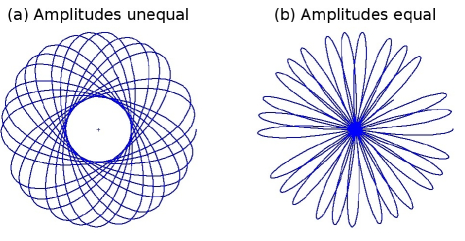
Figure 11: Two epicyclic orbits. (a) Amplitudes unequal: $\mu_{1}=1.0$, $\mu_{2}=2.0$. (b) Amplitudes equal: $\mu_{1}=\mu_{2}=1.0$. In both cases, $\beta_{1}=1.0$ and $\beta_{2}=\pi^{2}/8$.

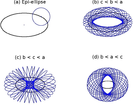
Figure 12: (a) Inner ellipse with major and minor semi-axes $a$ and $b$. Outer ellipse taken as a circle of radius $c$. (b) $c<b<a$: loop orbit. (c) $b<c<a$: box orbit. (d) $b<a<c$: loop orbit. In all cases, $\beta_{1}=1.0$ and $\beta_{2}=\pi^{2}/8$. The inner ellipse is shown as a heavy curve in each panel.

Epi-elliptic motion

The solution (37)–(38) has two components, each being a trajectory that is elliptic The first component is

$$\mu=\mu_{1}\cos[\beta_{1}(t-t_{1})]\,,\qquad\nu=\nu_{1}\sin[\beta_{1}(t-t_{1})]\,,$$

elliptical motion with frequency $\beta_{1}$ and semi-axes $\mu_{1}$ and $\nu_{1}=\mu_{1}\lambda_{1}$. The second component is

$$\mu=\mu_{2}\cos[\beta_{2}(t-t_{2})]\,,\qquad\nu=\nu_{2}\sin[\beta_{2}(t-t_{2})]\,,$$

elliptical motion with frequency $\beta_{2}$ and semi-axes $\mu_{2}$ and $\nu_{2}=\mu_{2}\lambda_{2}$. The character of the trajectory is thus determined by the relative magnitudes and signs of the parameters $\{\mu_{1},\nu_{1},\mu_{2},\nu_{2}\}$.

First, we consider the case where the second ellipse fits within the first:

$$|\mu_{1}|-|\mu_{2}|>0\qquad\mbox{and}\qquad|\nu_{1}|-|\nu_{2}|>0\,.$$

Clearly, $\varrho$ remains positive, with $\varrho_{\rm min}=\min\{(|\mu_{1}|-|\mu_{2}|),(|\nu_{1}|-|\nu_{2}|)\}$. There is an exclusion zone around the origin, inaccessible to the trajectory and we have a loop orbit. Next, we consider the case where the first ellipse fits within the second:

$$|\mu_{1}|-|\mu_{2}|<0\qquad\mbox{and}\qquad|\nu_{1}|-|\nu_{2}|<0\,.$$

Again, $\varrho$ is bounded away from zero and the trajectory is a loop orbit. The remaining case is where $(|\mu_{1}|-|\mu_{2}|)$ and $(|\nu_{1}|-|\nu_{2}|)$ are of opposite signs. Then $\varrho$ may become zero, the trajectory may pass through the origin and the orbit is of box type. Since it is only in this case that recession may be observed, the criterion for recession may be written

$$(|\mu_{1}|-|\mu_{2}|)\cdot(|\nu_{1}|-|\nu_{2}|)<0\,.$$ (39)

as stated in (26) in §4.

To illustrate the character of the orbits, we plot some solutions in Fig 12. We let the major and minor semi-axes of the inner ellipse be $a$ and $b$ and those of the outer ellipse be $c$ and $d$. Without loss of generality, we take $c=d$. Then the three cases discussed above are presented in panels (b), (c) and (d) of Fig 12. The criterion (39) for box orbits in this case is $b<c<a$. Clearly, loop orbits obtain for $c<b$ and for $c>a$.

There is a simple geometric interpretation of the criterion (39) for box orbits and recession: it requires that, if the two ellipses are drawn with a common centre, they intersect each other.

Squaring the circle

The domain of the the orbit (1)–(2) of the simple harmonic oscillator, in the generic case of irrational $\delta^{\prime}$, is dense in a rectangular area. If, for simplicity, we assume $x_{0}=y_{0}$, the orbit covers a square. It is not immediately obvious how this may be expressed in terms of epi-elliptic motion. However, let us assume that $\nu_{1}=\mu_{2}=0$, so that the elliptic components degenerate into two orthogonal line segements and the solution (37)–(38) becomes

$$\mu=\mu_{1}\cos\beta_{1}(t-t_{1})\,,\qquad\nu=\nu_{2}\sin\beta_{2}(t-t_{2})\,.$$

This is isomorphic to the solution (1)–(2). Thus, the circle is squared.

References

References

- [1] Altmann S.L., 1986: Rotations, Quaternions and Double Groups. Dover Publ. Inc., New York, 317pp.
- [2] Arnold, V.I., 1978: Mathematical Methods of Classical Mechanics Springer-Verlag, New York, Heidelberg, Berlin, 462pp.
- [3] Binney, James and Scott Tremaine, 2008: Galactic Dynamics Princeton Univ. Press, Princeton and Oxford. 885pp.
- [4] Bobylev, D.K., 1892: On a sphere with a gyroscope inside. Mathematical Collection of the Moscow Mathematical Society 16 (1892) 544–581 (in Russian).
- [5] Borisov, A.V., A.A. Kilin, and I.S. Mamaev, 2006: New Effects in Dynamics of Rattlebacks Dokl. Phys, 51, 272–275.
- [6] Borisov, A.V. and I.S. Mamaev, 2002: Rolling of a rigid body on a plane and a sphere. Hierarchy of dynamics. Regular and Chaotic Dynamics, 7 (2), 177–200.
- [7] Chaplygin, S.A., 1897: On a motion of a heavy body of revolution on a horizontal plane. Proc. of the Physical Sciences section of the Society of Amateurs of Natural Sciences, v. IX, 1897. English translation in Regular and Chaotic Dynamics 7, No. 2 (2002) 119–130.
- [8] Chaplygin, S.A., 1903: On a sphere rolling on a horizontal plane. Mathematical Collection of the Moscow Mathematical Society 24, 139–168. English translation in Regular and Chaotic Dynamics, 7, No. 2 (2002), 131–148. DOI: 10.1070/RD2002v007n02ABEH000200
- [9] Cushman, R., 1998: Routh’s sphere. Rep. Math. Phys., 42 (1-2), 47–70.
- [10] Duistermaat, J.J., 2004: Chaplygin’s Sphere arXiv:math.DS/0409019 v1 1 Sep 2004
- [11] Goldstein H., C. Poole and J. Safko, 2002: Classical Mechanics, 3rd Edn., Addison-Wesley, 638pp.
- [12] Gray, C.G. and B.G. Nickel, 2000: Constants of the motion for nonslipping tippe tops and other tops with round pegs. Am. J. Phys.,, 68, 821–8.
- [13] Holm, Darryl D., 2011: Geometric Mechanics. Part II: Rotating, Translating and Rolling, 2nd Edn., Imperial Coll. Press, London, 390pp.
- [14] Kim, Byungsoo, 2011: Routh symmetry in the Chaplygin’s rolling ball. Regular and Chaotic Dynamics, 16, No. 6, 663–670.
- [15] Kilin, A.A., 2001: The dynamics of Chaplygin ball: the qualitative and computer analysis. Regular and Chaotic Dynamics, 6, No. 3, 291–306. DOI: 10.1070/RD2001v006n03ABEH000178
- [16] Koslov, V.V., 2002: On the integration theory of equations of nonholonomic mechanics. Regular and Chaotic Dynamics, 7, No. 2, 161–176. DOI: 10.1070/RD2002v007n02ABEH000203
- [17] Kuipers, J.B., 1999: Quaternions and Rotation Sequences. Princeton Univ. Press, 371pp.
- [18] Landau, L.D. and E.M. Lifshitz, 1976: Course of Theoretical Physics, Vol 1: Mechanics. 3rd Edn. Elsevier, 170pp.
- [19] Lynch, P. and M.D. Bustamante, 2009: Precession and Recession of the Rock’n’roller. J. Phys. A: Math. Theor., 42 425203 (25pp). DOI: 10.1088/1751-8113/42/42
- [20] Marsden, J.E. and T.S. Ratiu, 1999: Introduction to Mechanics and Symmetry. 2nd Edn., Springer, 582pp.
- [21] Routh, E.J., 1905: A Treatise on the Dynamics of a System of Rigid Bodies, Part II: The Advanced Part. 6th Edition, Macmillan & Co New York. Reprint: Dover, New York, 1955.
- [22] Synge, J.L. & B.A. Griffith 1959: Principles of Mechanics, 3rd Edn, 552pp. McGraw Hill.
- [23] Whitham, G.B., 1974: Linear and Nonlinear Waves. Wiley-Interscience, New York, 651 pp.
- [24] Whittaker, E.T., 1937 A Treatise on the Analytical Dynamics of Particles and Rigid Bodies. 4th Edn., Cambridge Univ. Press, 456pp.