Quantitative test of the time dependent Gintzburg-Landau equation for sheared granular flow in two dimension

Abstract

We examine the validity of the time-dependent Ginzburg-Landau equation of granular fluids for a plane shear flow under the Lees-Edwards boundary condition derived from a weakly nonlinear analysis through the comparison with the result of discrete element method. We verify quantitative agreements in the time evolutions of the area fraction and the velocity fields, and also find qualitative agreement in the granular temperature.

I Introduction

Flows of granular particles have been extensively studied due to the importance in powder technology, civil engineering, mechanical engineering, geophysics, astrophysics, applied mathematics and physics Luding (2009); Pöschel and Luding (2001); Brilliantov and Pöschel (2004); Goldhirsch (2003). The characteristic properties of the granular flows are mainly caused by the inelastic collisions Jeager et al. (1996). In particular, the study of granular gases under a plane shear plays an important role in the application of the kinetic theory Sela et al. (1996); Santos et al. (2004); Lun (1991); Brey et al. (1998); Garzó and Dufty (1998); Lutsko (2004, 2005, 2006); Jenkins and Richman (1985a, b), the shear band or the plug in a moderate dense flow Tan and Goldhirsch (1997); Saitoh and Hayakawa (2007a), the long-time tail and the long-range correlations Kumaran (2006, 2009a, 2009b); Orpe and Kudrolli (2007); Orpe et al. (2008); Rycroft et al. (2009); Lutsko and Dufty (1985); Otsuki and Hayakawa (2009a, b, c), the pattern formation of dense flow Louge (1994, 2003); Xu et al. (2004, 2003); Khain (2007, 2009), the determination of the constitutive equation for dense flow Midi (2004); da Cruz et al. (2005); Hatano (2007), as well as jamming transition van Hecke (2010); Hatano et al. (2007); Hatano (2008); Otsuki and Hayakawa (2009d, e); Otsuki et al. (2010); Otsuki and Hayakawa (2011).

The granular hydrodynamic equations based on the kinetic theory well describe the dynamics of moderate dense granular gases Lun (1991); Brey et al. (1998); Garzó and Dufty (1998); Lutsko (2004, 2005, 2006); Jenkins and Richman (1985a, b), even though its applicability is questionable because of the lack of scale separation and the existence of long range correlations, etc. The two-dimensional granular shear flow is an appropriate target to check the validity of the granular hydrodynamic equations, where two denser regions are formed near the boundaries and collide to form a single dense plug under a physical boundary condition Tan and Goldhirsch (1997); Saitoh and Hayakawa (2007a). We refer the dense plugs as shear bands throughout this paper (even though ”shear-band” is often referred to the region of lower density with higher shear rate in the literature of engineering). A similar shear band is also observed under the Lees-Edwards boundary condition. The transient dynamics of the shear band and the hydrodynamic fields can be described by the granular hydrodynamic equations, where reasonable agreements with the discrete element method (DEM) simulation have been verified Saitoh and Hayakawa (2007a). It is also known that a homogeneous state of the two-dimensional granular shear flow is intrinsically unstable as predicted by the linear stability analysis Savage (1992); Garzó (2006); Schmid and Kytömaa (1994); Wang et al. (1996); Alam and Nott (1997, 1998); Gayen and Alam (2006).

To understand the shear band formation after the homogeneous state becomes unstable, we have to develop the weakly nonlinear analysis. Recently, Shukla and Alam carried out a weakly nonlinear analysis of the sheared granular flow in finite size systems, where they derived the Stuart-Landau equation for the disturbance amplitude of the hydrodynamic fields under a physical boundary condition Shukla and Alam (2009, 2011a, 2011b); Alam and Shukla (2012); Alam (2012). They found the existence of subcritical bifurcation in both dilute and dense regimes, while a supercritical bifurcation appears in the medium regime and the extremely dilute regime. The Stuart-Landau equation, however, does not include any spatial degrees of freedom and cannot be used to study the slow evolution of the spatial structure of shear band. We also notice that the shear rate is fixed to unity and cannot be used as a control parameter in their analysis.

It is also notable that several authors found coexistence of solid and liquid phases in their molecular dynamics simulations of dense granular shear flows Khain (2007, 2009); Alam and Luding (2003); Alam et al. (2005, 2008); Nott et al. (1999). In particular, Khain showed a hysteresis loop of the order parameter defined as a density contrast between the boundary and the center region Khain (2007, 2009). It should be noted, however, that the mechanism of the subcritical bifurcation based on a set of hydrodynamic equations differs from that observed in the jamming transition of frictional particles Otsuki and Hayakawa (2011). Indeed, the hysteresis loop in the jamming, which is observed for polydisperse grains, is originated from the frustrated and metastable configurations of frictional grains, while the hysteresis for monodisperse grains observed by Khain is from the coexistence of a crystal structure and a liquid structure.

In our previous work, we have developed the weakly nonlinear analysis for the two-dimensional granular shear flow and derived the time dependent Ginzburg-Landau (TDGL) equation for the disturbance amplitude. We introduced a hybrid approach to the weakly nonlinear analysis, where the derived TDGL equation is written as a two-dimensional form and has time dependent diffusion coefficients Saitoh and Hayakawa (2007b). We have also discussed the bifurcation of the amplitude, however, the studies of the numerical solution of the TDGL equation and comparison with the DEM simulation had been left as an incomplete part of our previous paper Saitoh and Hayakawa (2007b). Part of this study without comparison with DEM simulation has been published in another paper Saitoh and Hayakawa (2012)

In this paper, we quantitatively examine the validity of the derived TDGL equation for a two dimensional granular shear flow from the comparison with the DEM simulation. In Sec. II, we review the weakly nonlinear analysis and the hybrid approach. In Sec. III, which is the main part of this paper, we compare the numerical solutions of the TDGL equation with the results of DEM simulation. In Sec. IV, we discuss and conclude our results.

II Overview of weakly nonlinear analysis

In this section, we review our previous results for the weakly nonlinear analysis, where the time evolution for the disturbance amplitude is described by the TDGL equation Saitoh and Hayakawa (2007b). We also apply the hybrid approach to the TDGL equation to describe the structural changes of the shear band Saitoh and Hayakawa (2007b). In Sec. II.1, we introduce the basic equations. In Sec. II.2, we review the weakly nonlinear analysis to derive the TDGL equation. In Sec. II.3, we derive a two-dimensional TDGL equation adopting the hybrid approach to the weakly nonlinear analysis.

II.1 Basic equations

Let us explain our setup and basic equations. To avoid difficulties caused by the physical boundary condition, we adopt the Lees-Edwards boundary condition Lees and Edwards (1972), where the upper and the lower image cells move to the opposite directions with a constant speed $U/2$. Here, the distance between the upper and the lower image cells is given by $L$. We assume that the granular disks are identical, where the mass, the diameter and the restitution coefficient are respectively given by $m$, $d$ and $e$. In the following argument, we scale the mass, the length and the time by $m$, $d$ and $2d/U$, respectively. Therefore, the shear rate $U/L$ is nondimensionalized as $\epsilon\equiv 2d/L$ which becomes a small parameter in the hydrodynamic limit $L\gg d$.

We employ a set of hydrodynamic equations of granular disks derived by Jenkins and Richman Jenkins and Richman (1985a). Although their original equations include the angular momentum and the spin temperature, it is known that the spin effects are localized near the boundary Mitarai et al. (2002) and the effect of rotation can be absorbed in the normal restitution coefficient, if the friction constant is small Jenkins and Zhang (2002); Yoon and Jenkins (2005); Saitoh and Hayakawa (2007a). Thus, our system is reduced to a system without the spin effects and the dimensionless hydrodynamic equations are given by

$$\left(\partial_{t}+\mathbf{v}\cdot\nabla\right)\nu = -\nu\nabla\cdot\mathbf{v}$$ (1)

$$\nu\left(\partial_{t}+\mathbf{v}\cdot\nabla\right)\mathbf{v} = -\nabla\cdot\mathsf{P}$$ (2)

$$\left(\nu/2\right)\left(\partial_{t}+\mathbf{v}\cdot\nabla\right)\theta = -\mathsf{P}:\nabla\mathbf{v}-\nabla\cdot\mathbf{q}-\chi~{},$$ (3)

where $\nu$, $\mathbf{v}=(u,w)$, $\theta$, $t$ and $\nabla=(\partial/\partial_{x},\partial/\partial_{y})$ are the area fraction, the dimensionless velocity fields, the dimensionless granular temperature, the dimensionless time and the dimensionless gradient, respectively. The pressure tensor $\mathsf{P}=(P_{ij})$, the heat flux $\mathbf{q}$ and the energy dissipation rate $\chi$ are given in the dimensionless forms as

$$P_{ij} = \left[p(\nu)\theta-\xi(\nu)\theta^{1/2}\left(\nabla\cdot\mathbf{v}\right)\right]\delta_{ij}-\eta(\nu)\theta^{1/2}e_{ij}~{},$$ (4)

$$\mathbf{q} = -\kappa(\nu)\theta^{1/2}\nabla\theta-\lambda(\nu)\theta^{3/2}\nabla\nu~{},$$ (5)

$$\chi = \frac{1-e^{2}}{4\sqrt{2\pi}}\nu^{2}g(\nu)\theta^{1/2}\left[4\theta-3\sqrt{\frac{\pi}{2}}\theta^{1/2}\left(\nabla\cdot\mathbf{v}\right)\right]~{},$$ (6)

respectively, where $p(\nu)\theta$, $\xi(\nu)\theta^{1/2}$, $\eta(\nu)\theta^{1/2}$, $\kappa(\nu)\theta^{1/2}$ and $\lambda(\nu)\theta^{3/2}$ are the dimensionless forms of the static pressure, the bulk viscosity, the shear viscosity, the heat conductivity and the coefficient associated with the gradient of density, respectively, and $e_{ij}\equiv(\nabla_{j}v_{i}+\nabla_{i}v_{j}-\delta_{ij}\nabla\cdot\mathbf{v})/2$ $(i,j=x,y)$ is the deviatoric part of the strain rate tensor. The explicit forms of them are listed in Table 1, where we adopt the radial distribution function at contact

$$g(\nu)=\frac{1-7\nu/16}{\left(1-\nu\right)^{2}}~{},$$ (7)

which is only valid for $\nu<0.7$ Verlet and Levesque (1982); Henderson (1977, 1975); Carnahan and Starling (1969).

$p(\nu)$	$=$	$\frac{1}{2}\nu\left[1+(1+e)\nu g(\nu)\right]$
$\xi(\nu)$	$=$	$\frac{1}{\sqrt{2\pi}}(1+e)\nu^{2}g(\nu)$
$\eta(\nu)$	$=$	$\sqrt{\frac{\pi}{2}}\left[\frac{g(\nu)^{-1}}{7-3e}+\frac{(1+e)(3e+1)}{4(7-3e)}\nu+\left(\frac{(1+e)(3e-1)}{8(7-3e)}+\frac{1}{\pi}\right)(1+e)\nu^{2}g(\nu)\right]$
$\kappa(\nu)$	$=$	$\sqrt{2\pi}\left[\frac{g(\nu)^{-1}}{(1+e)(19-15e)}+\frac{3(2e^{2}+e+1)}{8(19-15e)}\nu+\left(\frac{9(1+e)(2e-1)}{32(19-15e)}+\frac{1}{4\pi}\right)(1+e)\nu^{2}g(\nu)\right]$
$\lambda(\nu)$	$=$	$-\sqrt{\frac{\pi}{2}}\frac{3e(1-e)}{16(19-15e)}\left[4(\nu g(\nu))^{-1}+3(1+e)\right]\frac{d\left(\nu^{2}g(\nu)\right)}{d\nu}$

Table 1: The functions in Eqs.(4)-(6).

II.2 Weakly nonlinear analysis

To study the slow dynamics of shear band, we need to develop a weakly nonlinear analysis. For this purpose, we introduce a long time scale $\tau\equiv\epsilon^{2}t$ and long length scales $(\xi,\zeta)\equiv\epsilon(x,y)$. We also introduce the neutral solution around the most unstable mode $\mathbf{q}_{c}=(0,q_{c})$ as

$$\hat{\phi}_{\mathrm{n}}=A^{\rm L}(\zeta,\tau)\phi^{\rm L}_{q_{c}}e^{iq_{c}\zeta}+\mathrm{c.c.}~{},$$ (8)

where $\mathrm{c.c.}$ represents the complex conjugate and $\phi^{\rm L}_{q_{c}}$ corresponds to the Fourier coefficient of the hydrodynamic fields at $\mathbf{q}_{c}$. We notice that the amplitude of the layering mode $A^{\rm L}(\zeta,\tau)$ depends on $\zeta$ but is independent of $\xi$, because any non-layering modes $q_{x}\neq 0$ are linearly stable. Then, we expand $A^{\rm L}(\zeta,\tau)$ into the series of $\epsilon$ as

$$A^{\rm L}(\zeta,\tau)=\epsilon A^{\rm L}_{1}+\epsilon^{2}A^{\rm L}_{2}+\epsilon^{3}A^{\rm L}_{3}+\dots~{}.$$ (9)

Substituting Eqs. (8) and (9) into the hydrodynamic equations (1)-(3) and collecting terms in each order of $\epsilon$, we obtain an amplitude equation.

The first non-trivial equation at $O(\epsilon^{3})$ is the TDGL equation

$$\partial_{\tau}A^{\rm L}_{1}=\sigma_{c}A^{\rm L}_{1}+D\partial_{\zeta}^{2}A^{\rm L}_{1}+\beta A^{\rm L}_{1}|A^{\rm L}_{1}|^{2},$$ (10)

where $D$ and $\beta$ are listed in Table 2 of Ref. Saitoh and Hayakawa (2007b). Here, $\sigma_{c}$ is the maximum growth rate at $\mathbf{q}_{c}$ scaled by $\epsilon^{2}$. Because of the scaling relations $D=\bar{D}$ and $\beta=\epsilon\bar{\beta}$, we can rewrite the TDGL equation as the equation for the scaled amplitude $\bar{A}^{\rm L}_{1}\equiv\epsilon^{1/2}A^{\rm L}_{1}$ as

$$\partial_{\tau}\bar{A}^{\rm L}_{1}=\sigma_{c}\bar{A}^{\rm L}_{1}+\bar{D}\partial_{\zeta}^{2}\bar{A}^{\rm L}_{1}+\bar{\beta}\bar{A}^{\rm L}_{1}|\bar{A}^{\rm L}_{1}|^{2}~{}.$$ (11)

It should be noted that the TDGL equation (10) or (11) can be only used for $\beta,\bar{\beta}<0$, i.e., the case of a supercritical bifurcation.

Developing a similar procedure till $O(\epsilon^{5})$, we also obtain the amplitude equation

$$\partial_{\tau}\check{A}^{\rm L}=\sigma_{c}\check{A}^{\rm L}+\bar{D}\partial_{\zeta}^{2}\check{A}^{\rm L}+\bar{\beta}\check{A}^{\rm L}|\check{A}^{\rm L}|^{2}+\epsilon\bar{\gamma}\check{A}^{\rm L}|\check{A}^{\rm L}|^{4}+O(\epsilon^{3})~{},$$ (12)

where we have introduced $\check{A}^{\rm L}(\zeta,\tau)=\epsilon^{1/2}[A^{\rm L}_{1}(\zeta,\tau)+\epsilon A^{\rm L}_{2}(\zeta,\tau)+\epsilon^{2}A^{\rm L}_{3}(\zeta,\tau)]$ and $\bar{\gamma}$ is also listed in Table 2 of Ref. Saitoh and Hayakawa (2007b). Equation (12) can be used for $\bar{\beta}>0$ and $\bar{\gamma}<0$, i.e., the case of a subcritical bifurcation.

II.3 Hybrid approach to the weakly nonlinear analysis

Although we derived the TDGL equations (11) and (12), these equations do not include $\xi$ and they are still not appropriate to study the two-dimensional structure of shear band. Therefore, we need a new approach, where the non-layering mode is coupled with the layering mode. For this purpose, we add a small deviation to the most unstable mode as $\mathbf{q}(\tau)=\mathbf{q}_{c}+\delta\mathbf{q}(\tau)$ and assume $\hat{\phi}_{\mathrm{n}}$ does not change if the deviation $\delta\mathbf{q}(\tau)$ is small. Then, Eq. (8) can be rewritten as

$$\hat{\phi}_{\mathrm{n}}\simeq A^{\rm L}(\xi,\zeta,\tau)\phi^{\rm L}_{q_{c}}e^{i\mathbf{q}(\tau)\cdot\mathbf{z}}+\mathrm{c.c.}~{},$$ (13)

where we have introduced $\mathbf{z}\equiv(\xi,\zeta)$ and a $\xi$-dependent amplitude $A^{\rm L}(\xi,\zeta,\tau)$. If we also take into account the contribution from the non-layering mode, a hybrid solution is given by

$$\hat{\phi}_{\mathrm{h}} = \left\{A^{\rm L}(\xi,\zeta,\tau)\phi^{\rm L}_{q_{c}}+A^{\rm NL}(\xi,\zeta,\tau)\phi^{\rm NL}_{\mathbf{q}(\tau)}\right\}e^{i\mathbf{q}(\tau)\cdot\mathbf{z}}+\mathrm{c.c.}$$ (14)

$$\simeq A(\xi,\zeta,\tau)\left\{\phi^{\rm L}_{q_{c}}+\phi^{\rm NL}_{\mathbf{q}(\tau)}\right\}e^{i\mathbf{q}(\tau)\cdot\mathbf{z}}+\mathrm{c.c.}~{},$$

where $A^{\rm NL}(\xi,\zeta,\tau)$ and $\phi^{\rm NL}_{\mathbf{q}(\tau)}$ are the amplitude and the Fourier coefficient of the non-layering mode, respectively. Here, we have used a strong assumption that $A^{\rm L}(\xi,\zeta,\tau)$ and $A^{\rm NL}(\xi,\zeta,\tau)$ are scaled by a common amplitude $A(\xi,\zeta,\tau)$ in the second line of Eq. (14). Expanding $A(\xi,\zeta,\tau)$ as

$$A(\xi,\zeta,\tau)=\epsilon A_{1}(\xi,\zeta,\tau)+\epsilon^{2}A_{2}(\xi,\zeta,\tau)+\epsilon^{3}A_{3}(\xi,\zeta,\tau)+\dots~{},$$ (15)

and carrying out the weakly nonlinear analysis for the hybrid solution $\hat{\phi}_{\mathrm{h}}$, we found the rescaled amplitude $\bar{A}_{1}(\xi,\zeta,\tau)\equiv\epsilon^{1/2}A_{1}(\xi,\zeta,\tau)$ for the supercritical bifurcation satisfies

$$\partial_{\tau}\bar{A}_{1}=\sigma_{c}\bar{A}_{1}+\bar{D}_{1}(\tau)\partial_{\xi}^{2}\bar{A}_{1}+\bar{D}_{2}(\tau)\partial_{\xi}\partial_{\zeta}\bar{A}_{1}+\bar{D}\partial_{\zeta}^{2}\bar{A}_{1}+\bar{\beta}\bar{A}_{1}|\bar{A}_{1}|^{2}$$ (16)

at $O(\epsilon^{3})$, where $\bar{D}_{1}(\tau)$ and $\bar{D}_{2}(\tau)$ are the time dependent diffusion coefficients. Similarly, we found the higher order equation of $\check{A}(\xi,\zeta,\tau)\equiv\epsilon^{1/2}\{A_{1}(\xi,\zeta,\tau)+\epsilon A_{2}(\xi,\zeta,\tau)+\epsilon^{2}A_{3}(\xi,\zeta,\tau)\}$ as

$$\partial_{\tau}\check{A}=\sigma_{c}\check{A}+\bar{D}_{1}(\tau)\partial_{\xi}^{2}\check{A}+\bar{D}_{2}(\tau)\partial_{\xi}\partial_{\zeta}\check{A}+\bar{D}\partial_{\zeta}^{2}\check{A}+\bar{\beta}\check{A}|\check{A}|^{2}+\epsilon\bar{\gamma}\check{A}|\check{A}|^{4}+O(\epsilon^{3})$$ (17)

for the subcritical bifurcation. The time dependent diffusion coefficients $\bar{D}_{1}(\tau)$ and $\bar{D}_{2}(\tau)$ whose explicit forms are given by Eqs. (64) and (65) in Ref. Saitoh and Hayakawa (2007b) decay to zero as time goes on. Therefore, Eqs. (16) and (17) are respectively reduced to Eqs. (11) and (12) in the long time limit.

III Discrete element method (DEM) simulation

In this section, we perform the discrete element method (DEM) simulation for a two-dimensional granular shear flow to compare the results with the weakly nonlinear analysis. In Sec. III.1, we introduce our setup and in Sec. III.2, we show the time evolution of the density field obtained from the DEM simulation, where the typical transient dynamics can be reproduced. In Sec. III.3, we exhibit the time evolution of the velocity fields and the granular temperature, and in Sec. III.4, we compare the results of the DEM simulation with the numerical solution of the TDGL equation. In the following, we use the same units of mass, length and time as those in the weakly nonlinear analysis.

In Eq. (16), $\bar{\beta}<0$ for $\nu_{0}<0.245$ where the supercritical bifurcation is expected Saitoh and Hayakawa (2007b). If $0.245<\nu_{0}<0.275$, $\bar{\beta}>0$ and $\bar{\gamma}<0$, thus Eq. (17) should be used and the subcritical bifurcation is expected. Unfortunately, $\bar{\beta}>0$ and $\bar{\gamma}>0$ for $\nu_{0}>0.275$ and neither Eqs. (16) nor (17) can be used. Therefore, we exhibit our numerical results with $\nu_{0}=0.18$ and $0.26$ for the supercritical and subcritical cases, respectively.

III.1 Setup

We adopt the linear spring-dashpot model, where the normal force between the colliding two particles is given by $f_{n}=k_{n}\delta-\eta_{n}\dot{\delta}$ with the overlap $\delta$ and the relative speed $\dot{\delta}$. For simplicity, we ignore the tangential contact force, because we have already verified the results are unchanged for the realistic value of the friction coefficient by introducing the effective restitution coefficient Yoon and Jenkins (2005); Saitoh and Hayakawa (2007a). In our simulation, we adopt that the spring and viscosity constants are respectively $k_{n}=500mU^{2}/d^{2}$ and $\eta_{n}=1.0mU/d$. In this case, the normal restitution coefficient given by

$$e=\exp\left[-\frac{\pi}{\sqrt{2mk_{n}/\eta_{n}^{2}-1}}\right]$$ (18)

becomes $e\simeq 0.9$ whose value may not be sufficiently large to ensure elastic limit Luding (2008, 2005). We adopt that the periodic boundary condition and the Lees-Edwards boundary condition with the relative speed $U$ for the boundaries of the $\xi$- and $\zeta$-axes, respectively. Then, we randomly distribute $N=8192$ particles in a $L^{\ast}\times L^{\ast}$ square box with the dimensionless system size $L^{\ast}\equiv L/d=189$ ($\nu_{0}=0.18$) and $155$ ($\nu_{0}=0.26$), respectively, and randomly distribute the initial velocities around the linear velocity profile with the dimensionless shear rate $\epsilon\simeq 10^{-2}$.

III.2 Shear band formation

Figure 1 (upper panel) displays the time evolution of particles in the DEM simulation for $\nu_{0}=0.18$. The corresponding hydrodynamic fields can be obtained by the coarse graining (CG) procedure developed by Goldhirsch et. al. Glasser and Goldhirsch (2001); Goldenberg and Goldhirsch (2002); Goldhirsch and Goldenberg (2002); Goldenberg and Goldhirsch (2004, 2005); Goldenberg et al. (2006); Goldhirsch (2010); Zhang et al. (2010); Clark et al. (2012); Weinhart et al. (2012), where the CG function is defined as $\psi(\mathbf{z})=e^{-\mathbf{z}^{2}}/\pi$ at $\mathbf{z}=(\xi,\zeta)$. Figure 1 (middle panel) shows the time evolution of the area fraction defined as

$$\nu_{\mathrm{DEM}}(\mathbf{z},\tau)=\frac{\pi}{4}\sum_{i=1}^{N}\psi(\mathbf{z}-\mathbf{z}_{i})~{},$$ (19)

where $\mathbf{z}_{i}=(\xi_{i},\zeta_{i})$ is the dimensionless position of $i$-th disk. Figure 1 (lower panel) shows the numerical solution of Eq. (16).

In Fig. 1, a typical transient dynamics exhibits that (a) the fluctuation with the short wave length is suppressed, (b) clusters are generated and merged, and (c) the shear band is generated and the system reaches a steady state. Such transient dynamics of shear band is qualitatively similar to the numerical solution of Eq. (16). We should stress that these results cannot be explained by neither the one-dimensional TDGL equation nor zero-dimensional Stuart-Landau equation obtained by the ordinary weakly nonlinear analysis Shukla and Alam (2009, 2011a, 2011b).

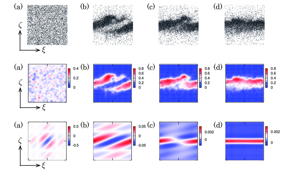
Figure 1: (Color online) Upper panel: Time evolution of particles in the DEM simulation, where $\nu_{0}=0.18$. Middle panel: Time evolution of $\nu_{\mathrm{DEM}}(\mathbf{z},\tau)$. Lower panel: Numerical solution of Eq. (16). Here, the dimensionless time corresponds to (a) $0$, (b) $4.8$, (c) $11.2$ and (d) $20.0$, respectively.

III.3 Velocity fields and granular temperature

The velocity fields and the granular temperature are defined as

$$\mathbf{u}_{\mathrm{DEM}}(\mathbf{z},\tau) = \frac{\sum_{i}\mathbf{v}_{i}\psi(\mathbf{z}-\mathbf{z}_{i})}{\sum_{i}\psi(\mathbf{z}-\mathbf{z}_{i})}~{},$$ (20)

$$\theta_{\mathrm{DEM}}(\mathbf{z},\tau) = \frac{\sum_{i}\mathbf{V}_{i}^{2}\psi(\mathbf{z}-\mathbf{z}_{i})}{2\sum_{i}\psi(\mathbf{z}-\mathbf{z}_{i})}~{},$$ (21)

respectively, where $\mathbf{v}_{i}$ and $\mathbf{V}_{i}=\mathbf{v}_{i}-\mathbf{u}_{\mathrm{DEM}}(\mathbf{z}_{i},\tau)$ are the dimensionless velocity of the $i$-th particle and the dimensionless local velocity, respectively. Figures 2 (upper panel), (middle panel) and (lower panel) display the time evolution of $u_{\mathrm{DEM}}(\mathbf{z},\tau)$, $w_{\mathrm{DEM}}(\mathbf{z},\tau)$ and $\theta_{\mathrm{DEM}}(\mathbf{z},\tau)$, respectively, where $u_{\mathrm{DEM}}(\mathbf{z},\tau)$ and $w_{\mathrm{DEM}}(\mathbf{z},\tau)$ are respectively the $\xi$ and $\zeta$ components of $\mathbf{u}_{\mathrm{DEM}}(\mathbf{z},\tau)$. As time goes on, $u_{\mathrm{DEM}}(\mathbf{z},\tau)$ in the $\zeta$ direction deviates from the linear profile and $w_{\mathrm{DEM}}(\mathbf{z},\tau)$ is almost homogeneous. The time evolution of $\theta_{\mathrm{DEM}}(\mathbf{z},\tau)$ is accompanied with $\nu_{\mathrm{DEM}}(\mathbf{z},\tau)$, where $\theta_{\mathrm{DEM}}(\mathbf{z},\tau)$ is lower in the dense region and higher in the dilute region.

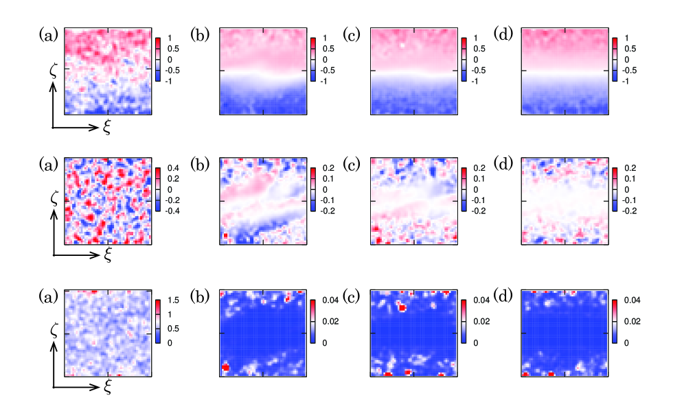
Figure 2: (Color online) Upper panel: Time evolution of $u_{\mathrm{DEM}}(\mathbf{z},\tau)$. Middle panel: Time evolution of $w_{\mathrm{DEM}}(\mathbf{z},\tau)$. Lower panel: Time evolution of $\theta_{\mathrm{DEM}}(\mathbf{z},\tau)$. Here, the dimensionless time corresponds to (a) $0$, (b) $4.8$, (c) $11.2$ and (d) $20.0$, respectively.

III.4 Comparison of the TDGL equation with the DEM simulation

To test the quantitative validity of the TDGL equation, we compare the numerical solution with the results of DEM simulation. At first, we average out $\nu_{\mathrm{DEM}}(\mathbf{z},\tau)$, $u_{\mathrm{DEM}}(\mathbf{z},\tau)$, $w_{\mathrm{DEM}}(\mathbf{z},\tau)$ and $\theta_{\mathrm{DEM}}(\mathbf{z},\tau)$ over the $\xi$ direction and take sample averages from the different $100$ time steps. Then, the hydrodynamic fields are written as one-dimensional forms $\nu_{\mathrm{DEM}}(\zeta,\tau)$, $u_{\mathrm{DEM}}(\zeta,\tau)$, $w_{\mathrm{DEM}}(\zeta,\tau)$ and $\theta_{\mathrm{DEM}}(\zeta,\tau)$, respectively. Because $\nu_{\mathrm{DEM}}(\zeta,\tau)$ and $\theta_{\mathrm{DEM}}(\zeta,\tau)$ are approximately symmetric at $\zeta=0$, we introduce

$$\bar{\nu}_{\mathrm{DEM}}(\zeta,\tau) \equiv \frac{1}{2}\left\{\nu_{\mathrm{DEM}}(\zeta,\tau)+\nu_{\mathrm{DEM}}(-\zeta,\tau)\right\}\hskip 14.22636pt(0<\zeta<L^{\ast}/2)~{},$$ (22)

$$\bar{\theta}_{\mathrm{DEM}}(\zeta,\tau) \equiv \frac{1}{2}\left\{\theta_{\mathrm{DEM}}(\zeta,\tau)+\theta_{\mathrm{DEM}}(-\zeta,\tau)\right\}\hskip 14.22636pt(0<\zeta<L^{\ast}/2)~{},$$ (23)

respectively. On the other hand, the velocity fields are approximately antisymmetric at $\zeta=0$ and we also introduce

$$\bar{u}_{\mathrm{DEM}}(\zeta,\tau) \equiv \frac{1}{2}\left\{u_{\mathrm{DEM}}(\zeta,\tau)-u_{\mathrm{DEM}}(-\zeta,\tau)\right\}\hskip 14.22636pt(0<\zeta<L^{\ast}/2)~{},$$ (24)

$$\bar{w}_{\mathrm{DEM}}(\zeta,\tau) \equiv \frac{1}{2}\left\{w_{\mathrm{DEM}}(\zeta,\tau)-w_{\mathrm{DEM}}(-\zeta,\tau)\right\}\hskip 14.22636pt(0<\zeta<L^{\ast}/2)~{},$$ (25)

respectively.

In the weakly nonlinear analysis, the hydrodynamic fields are given by the summation of the base state $\phi_{0}=(\nu_{0},\zeta,0,\theta_{0})$ and the hybrid solution $\hat{\phi}_{\mathrm{h}}$. At first, we project $\hat{\phi}_{\mathrm{h}}$ on the $\zeta$-axis as

$$\hat{\phi}_{\mathrm{h}}(\zeta,\tau)\simeq\bar{\bar{A}}(\zeta,\tau)\phi^{\rm L}_{q_{c}}e^{iq_{\zeta}(\tau)\zeta}+\mathrm{c.c.}~{},$$ (26)

where $q_{\zeta}(\tau)\equiv q_{c}-\tau$ is the $\zeta$ component of $\mathbf{q}(\tau)$ qze and we ignore $\phi^{\rm NL}_{\mathbf{q}(\tau)}$, because $\phi^{\rm NL}_{\mathbf{q}(\tau)}$ exponentially decays to zero and the following results are unchanged even if we take into account $\phi^{\rm NL}_{\mathbf{q}(\tau)}$. We note that $\phi^{\rm L}_{q_{c}}$ is defined as $\phi^{\rm L}_{q_{c}}=\left(\nu_{q_{c}},iu_{q_{c}},iw_{q_{c}},\theta_{q_{c}}\right)^{\mathrm{T}}$ with the imaginary unit $i$, where $\nu_{q_{c}}$, $u_{q_{c}}$, $w_{q_{c}}$ and $\theta_{q_{c}}$ are the Fourier coefficients of the area fraction, the velocity fields $u$ and $w$, and the granular temperature, respectively, and they are given in our previous paper Saitoh and Hayakawa (2007b). If we ignore the higher order terms in Eq. (15), $\bar{\bar{A}}(\zeta,\tau)$ may be given by the numerical solution of Eq. (16) projected on the $\zeta$-axis. Then, the hydrodynamic fields are given by $\phi_{\mathrm{TDGL}}(\zeta,\tau)=\phi_{0}+\hat{\phi}_{\mathrm{h}}(\zeta,\tau)$, where each component of $\phi_{\mathrm{TDGL}}(\zeta,\tau)$ is written as

$$\nu_{\mathrm{TDGL}}(\zeta,\tau) = \nu_{0}+2\nu_{q_{c}}\bar{\bar{A}}(\zeta,\tau)\cos(q_{\zeta}(\tau)\zeta)~{},$$ (27)

$$u_{\mathrm{TDGL}}(\zeta,\tau) = \zeta-2u_{q_{c}}\bar{\bar{A}}(\zeta,\tau)\sin(q_{\zeta}(\tau)\zeta)~{},$$ (28)

$$w_{\mathrm{TDGL}}(\zeta,\tau) = -2w_{q_{c}}\bar{\bar{A}}(\zeta,\tau)\sin(q_{\zeta}(\tau)\zeta)~{},$$ (29)

$$\theta_{\mathrm{TDGL}}(\zeta,\tau) = \theta_{0}+2\theta_{q_{c}}\bar{\bar{A}}(\zeta,\tau)\cos(q_{\zeta}(\tau)\zeta)~{},$$ (30)

respectively, where the factor $2$ comes from the complex conjugate.

Figures 3 and 4 display the time evolution of the hydrodynamic fields for the supercritical case ($\nu_{0}=0.18$) and the subcritical case ($\nu_{0}=0.26$), respectively, where the symbols represent Eqs. (22)-(25) obtained by the DEM simulation and the lines represent the scaling functions

$$\bar{X}_{\mathrm{TDGL}}(\zeta,\tau)\equiv a^{\ast}_{X}X_{\mathrm{TDGL}}(\zeta/\zeta^{\ast}_{X}(\tau),\tau/\tau^{\ast})\hskip 14.22636pt(X=\nu,u,w,\theta)$$ (31)

with the scaling factors $a^{\ast}_{X}$, $\zeta^{\ast}_{X}(\tau)$ and $\tau^{\ast}$, respectively. We quantify the difference between Eqs. (22)-(25) and Eq. (31) by introducing the relative standard deviation

$$\mathrm{Err.}\equiv\sqrt{\frac{\left(\bar{X}_{\mathrm{DEM}}-\bar{X}_{\mathrm{TDGL}}\right)^{2}}{\bar{X}_{\mathrm{TDGL}}^{2}}}\hskip 14.22636pt(X=\nu,u,w,\theta)~{},$$ (32)

where we omit the arguments $(\zeta,\tau)$. In Fig. 3(a)-(c), $\bar{\nu}_{\mathrm{TDGL}}(\zeta,\tau)$, $\bar{u}_{\mathrm{TDGL}}(\zeta,\tau)$ and $\bar{w}_{\mathrm{TDGL}}(\zeta,\tau)$ are quantitatively agreed with $\bar{\nu}_{\mathrm{DEM}}(\zeta,\tau)$, $\bar{u}_{\mathrm{DEM}}(\zeta,\tau)$ and $\bar{w}_{\mathrm{DEM}}(\zeta,\tau)$, respectively, where $\mathrm{Err.}$ is less than or equal to $0.1$. In Fig. 4 (a) and (b), $\bar{\nu}_{\mathrm{TDGL}}(\zeta,\tau)$ and $\bar{u}_{\mathrm{TDGL}}(\zeta,\tau)$ are quantitatively agreed with $\bar{\nu}_{\mathrm{DEM}}(\zeta,\tau)$ and $\bar{u}_{\mathrm{DEM}}(\zeta,\tau)$, respectively. We should note that we could not get any reasonable agreements between the $\zeta$ component of the velocity field even in a numerical solution of a set of the granular hydrodynamic equations and the result of DEM simulation in our previous work Saitoh and Hayakawa (2007a). We can also see the qualitative agreements in the $\zeta$ component of the velocity field for the subcritical case (Fig. 4(c)) and the granular temperature for the supercritical and subcritical cases (Figs. 3(d) and 4(d)), where $\mathrm{Err.}$ is less than or equal to $0.43$.

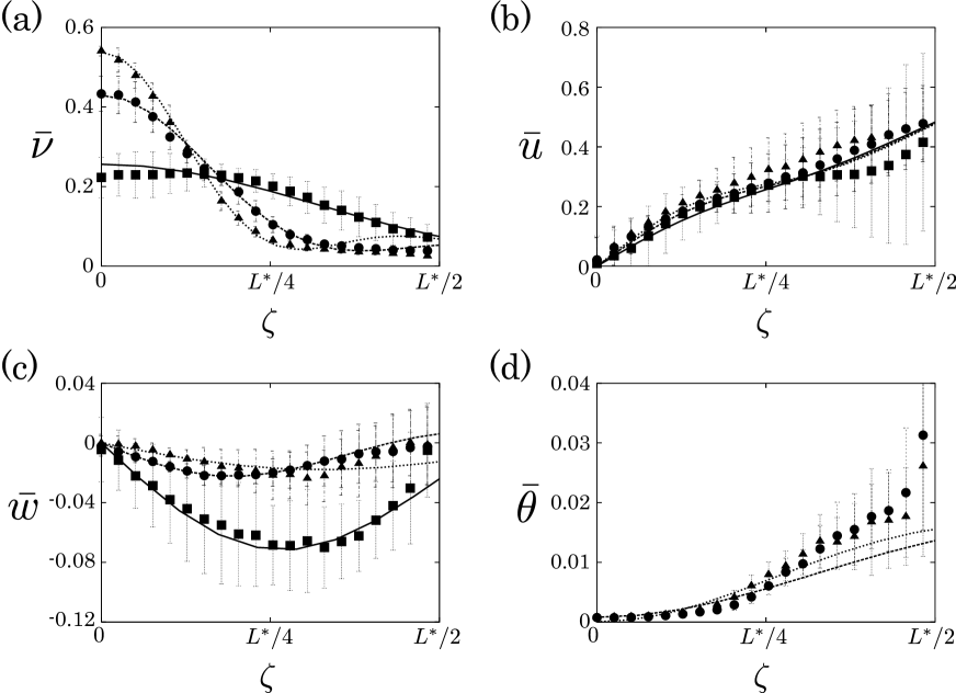
Figure 3: Time evolution of (a) $\bar{\nu}_{\mathrm{DEM}}(\zeta,\tau)$ and $\bar{\nu}_{\mathrm{TDGL}}(\zeta,\tau)$, (b) $\bar{u}_{\mathrm{DEM}}(\zeta,\tau)$ and $\bar{u}_{\mathrm{TDGL}}(\zeta,\tau)$, (c) $\bar{w}_{\mathrm{DEM}}(\zeta,\tau)$ and $\bar{w}_{\mathrm{TDGL}}(\zeta,\tau)$, (d) $\bar{\theta}_{\mathrm{DEM}}(\zeta,\tau)$ and $\bar{\theta}_{\mathrm{TDGL}}(\zeta,\tau)$, respectively, for the supercritical case ($\nu_{0}=0.18$), where the solid squares and the solid lines correspond to the dimensionless time $4.8$, the solid circles and the hashed lines correspond to the dimensionless time $11.2$, and the solid triangles and the dotted lines correspond to the dimensionless time $20.0$, respectively. Here, we have introduced the scaling factors $\tau^{\ast}\simeq 0.14$, $a^{\ast}_{\nu}\simeq 0.24$, $a^{\ast}_{u}\simeq 0.02$, $a^{\ast}_{w}\simeq 1.96$ and $a^{\ast}_{\theta}\simeq 0.02$, respectively, and we also use $\zeta_{\nu}^{\ast}(\tau)\simeq 1.6,0.9,0.75$, $\zeta_{u}^{\ast}(\tau)\simeq 0.8,0.8,0.8$, $\zeta_{w}^{\ast}(\tau)\simeq 1.5,1.1,1.8$ at the the dimensionless time $4.8$, $11.2$ and $20.0$, respectively, and $\zeta_{\theta}^{\ast}(\tau)\simeq 1.6,1.35$ at the dimensionless time $11.2$ and $20.0$, respectively. It should be noted that we do not show the result of the granular temperature at the dimensionless time $4.8$, because it homogeneously distributed around $\theta_{0}$ and the fluctuation is too large to plot in the same figure. Here, the relative standard deviations defined as Eq. (32) are (a) $0.09$, (b) $0.07$, (c) $0.10$ and (d) $0.35$, respectively.

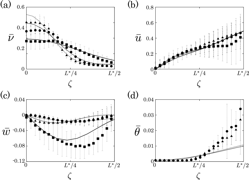
Figure 4: Time evolution of (a) $\bar{\nu}_{\mathrm{DEM}}(\zeta,\tau)$ and $\bar{\nu}_{\mathrm{TDGL}}(\zeta,\tau)$, (b) $\bar{u}_{\mathrm{DEM}}(\zeta,\tau)$ and $\bar{u}_{\mathrm{TDGL}}(\zeta,\tau)$, (c) $\bar{w}_{\mathrm{DEM}}(\zeta,\tau)$ and $\bar{w}_{\mathrm{TDGL}}(\zeta,\tau)$, (d) $\bar{\theta}_{\mathrm{DEM}}(\zeta,\tau)$ and $\bar{\theta}_{\mathrm{TDGL}}(\zeta,\tau)$, respectively, for the subcritical case ($\nu_{0}=0.26$), where we have used the same dimensionless time and the same scaling factors $\tau^{\ast}$, $a^{\ast}_{\nu}$, $a^{\ast}_{u}$, $a^{\ast}_{w}$, $a^{\ast}_{\theta}$, $\zeta_{\nu}^{\ast}(\tau)$, $\zeta_{u}^{\ast}(\tau)$, $\zeta_{w}^{\ast}(\tau)$ and $\zeta_{\theta}^{\ast}(\tau)$ in Fig. 3. Here, the relative standard deviations defined as Eq. (32) are (a) $0.10$, (b) $0.07$, (c) $0.40$ and (d) $0.43$, respectively.

IV Discussion and conclusion

In this paper, we examine the validity of the TDGL equation for a two-dimensional sheared granular flow from the comparison with the results of the DEM simulation by the CG method. The results of the TDGL equation, at least, qualitatively agree with the results of the DEM simulation. Such transient dynamics cannot be reproduced by neither the one dimensional TDGL equation nor the zero dimensional Stuart-Landau equation derived by the ordinary weakly nonlinear analysis. We also obtain that the velocity fields and the granular temperature qualitatively agree with the solution of the TDGL equation.

We compare the one dimensional hydrodynamic fields obtained from the DEM simulation with the scaled forms of the numerical solution of the TDGL equation, where we find the quantitative agreements in the area fraction and the $\xi$ component of the velocity field. In the supercritical regime, we also find the quantitative agreement in the $\zeta$ component of the velocity field. We can also observe the qualitative agreements in the $\zeta$ component of the velocity field for the subcritical case and the granular temperature for both the supercritical and subcritical cases. In our previous work, the hydrodynamic fields obtained from the DEM simulation are reasonably explained by the numerical solutions of the granular hydrodynamic equations by Jenkins and Richmann except for $w(\mathbf{z},\tau)$ Jenkins and Richman (1985a, b); Saitoh and Hayakawa (2007a). In the present work, even though we need to introduce the scaling factors, the results of the DEM simulation is qualitatively reproduced by the numerical solution of the TDGL equation. It is needless to say that more precise analyses will be important to remove the scaling factors. In addition, quantitative comparison with the DEM simulations in quasi elastic limit should be done in our future studies.

In conclusion, the numerical solution of the TDGL equation can qualitatively explain the time evolution of the hydrodynamic fields obtained by the DEM simulation.