Quasi-stars and the
Schönberg–Chandrasekhar limit
![[Uncaptioned image]](/html/1207.5972/assets/eds_bw.png)
![[Uncaptioned image]](/html/1207.5972/assets/ioa.png)
![[Uncaptioned image]](/html/1207.5972/assets/cam_bw.png)
Warrick Heinz Ball
St Edmund’s College
and
Institute of Astronomy
University of Cambridge
This dissertation is submitted for the degree of
Doctor of Philosophy
Declaration
I hereby declare that my dissertation entitled Quasi-stars and the Schönberg–Chandrasekhar limit is not substantially the same as any that I have submitted for a degree or diploma or other qualification at any other University.
I further state that no part of my dissertation has already been or is being concurrently submitted for any such degree, diploma or other qualification.
This dissertation is the result of my own work and includes nothing which is the outcome of work done in collaboration except as specified in the text. Those parts of this dissertation that have been published or accepted for publication are as follows.
- •
Parts of Chapters 1 and 2 and most of Chapter 3 have been published as
Ball, W. H., Tout, C. A., Żytkow, A. N., & Eldridge, J. J.
2011, MNRAS, 414, 2751- •
Material from Chapters 5 and 6 and Appendix A has been published as
Ball, W. H., Tout, C. A., Żytkow, A. N.,
2012, MNRAS, 421, 2713This dissertation contains fewer than 60 000 words.
Warrick Heinz Ball
Cambridge, May 29, 2012
Abstract
The mechanism by which the supermassive black holes that power bright quasars at high redshift form remains unknown. One possibility is that, if fragmentation is prevented, the monolithic collapse of a massive protogalactic disc proceeds via a cascade of triaxial instabilities and leads to the formation of a quasi-star: a growing black hole, initially of typical stellar-mass, embedded in a hydrostatic giant-like envelope. Quasi-stars are the main object of study in this dissertation. Their envelopes satisfy the equations of stellar structure so the Cambridge stars code is modified to model them. Analysis of the models leads to an extension of the classical Schönberg–Chandrasekhar limit and an exploration of the implications of this extension for the evolution of main-sequence stars into giants.
In Chapter 1, I introduce the problem posed by the supermassive black holes that power high-redshift quasars. I discuss potential solutions and describe the conditions under which a quasi-star might form. In Chapter 2, I outline the Cambridge stars code and the modifications that are made to model quasi-star envelopes.
In Chapter 3, I present models of quasi-stars where the base of the envelope is located at the Bondi radius of the black hole. The black holes in these models are subject to a robust upper fractional mass limit of about one tenth. In addition, the final black hole mass is sensitive to the choice of the inner boundary radius of the envelope. In Chapter 4, I construct alternative models of quasi-stars by drawing from work on convection- and advection-dominated accretion flows around black holes. To improve the accuracy of my models, I incorporate corrections owing to special and general relativity into a variant of the stars code that includes rotation. The evolution of these quasi-stars is qualitatively different from those described in Chapter 3. Most notably, the core black holes are no longer subject to a fractional mass limit and ultimately accrete all of the material in their envelopes.
In Chapter 5, I demonstrate that the fractional mass limit found in Chapter 3, for the black holes in quasi-stars, is in essence the same as the Schönberg–Chandrasekhar limit. The analysis demonstrates how other similar limits are related and that limits exist under a wider range of circumstances than previously thought. A test is provided that determines whether a composite polytrope is at a fractional mass limit. In Chapter 6, I apply this test to realistic stellar models and find evidence that the existence of fractional mass limits is connected to the evolution of stars into the red giants.
For dad, mom and Rudi.
Acknowledgements
First, I owe deep thanks to my supervisor, Chris Tout. His scientific insights are always invaluable. If I ever left our discussions without all the answers, I at least left with the right questions. I am also tremendously grateful to Anna Żytkow for her keen interest and extensive input. Her insistence on precise language has not only helped me keep my writing clear but my thinking too. I have also appreciated the continuing support of my MSc supervisor, Kinwah Wu, during my PhD and I owe him substantial thanks for his prompt responses to my various needs.
I would also like to thank the members of the Cambridge stellar evolution group who have come, been and gone during my time at the Institute. Particular thanks go to John Eldridge for being a sounding board during Chris’ sabbatical early in my studies, for helping me get to grips with the stars code and for his support in my applications to academic positions. I’d also like to thank my comrade-in-arms, Adrian Potter, not least for lending me his code, rose, but, owing to our common supervisor, being a willing ear for discussions regarding italicized axis labels and their units, hanging participles, and the Oxford comma. Thanks also to Richard Stancliffe for taking the time to respond to my confused emails, which were usually about a problem that existed between the seat and the keyboard.
On a personal note, I am tremendously thankful for my friendships, forged in Cambridge, in London or at home, that have endured my infrequent communication. I am also grateful for my fellow graduate students at the Institute who have come and gone during my degree. If anything, they have endured my frequent communication. Finally, to my family, thank you for providing inspiration, motivation and all manner of unconditional support to this marathon of mine.
Warrick Heinz Ball
Cambridge, May 29, 2012
[80mm]
‘Begin at the beginning,’ the King said gravely, ‘and go on till you
come to the end: then stop.’
\qauthorfrom Alice’s Adventures in Wonderland,
Lewis Carroll, 1865
Chapter 1 Supermassive
black holes
in the early Universe
Over the last decade, high-redshift surveys have detected bright quasars at redshifts (Fan et al. 2006; Jiang et al. 2008; Willott et al. 2010). Such observations imply that black holes (BHs) of more than were present less than after the Big Bang. A simple open question remains: how did these objects become so massive so quickly? Despite a large and growing body of investigation into the problem, no clear solution has yet been found (see Volonteri 2010, for a review).
Begelman, Volonteri & Rees (2006, hereinafter BVR06) proposed that the direct collapse of baryonic gas in a massive dark matter (DM) halo can lead to an isolated structure comprising an initially stellar-mass BH embedded in a hydrostatic envelope. Such structures were dubbed quasi-stars. At the centre of a quasi-star, a BH can grow faster than its own Eddington-limited rate. Quasi-stars can thus leave massive BH remnants that subsequently grow into the supermassive black holes (SMBHs) that power high-redshift quasars.
The structure of the gas around the BH is expected to obey the same equations as the envelopes of supergiant stars. In both cases, hydrostatic material surrounds a dense core. Giant envelopes are supported by radiation from nuclear reactions in or around the core whereas quasi-star envelopes are supported by radiation from accretion on to the BH. By choosing suitable interior conditions to describe the interaction of the BH and the envelope, it is possible to model a quasi-star with software packages designed to calculate stellar structure and evolution. Such an undertaking was the initial aim of the work described in this dissertation and the results ultimately shed new light on the structure of giant stars.
The purpose of this chapter is to provide the background for my work on quasi-stars. In Section 1.1, I provide a synopsis of progress in explaining the existence of high-redshift BHs and I explain the place of quasi-stars within our present understanding of the early Universe. In Section 1.2, I describe the structure and evolution of the first luminous objects in the Universe and the remnants they are expected to leave. Finally, in Section 1.3, I outline the layout of the rest of this dissertation.
1.1 Supermassive black hole formation
It is broadly accepted that the intense radiation from quasars is produced by material falling on to massive BHs (Salpeter 1964). To understand how and where such objects came to be, I first outline the current understanding of cosmic structure formation and then describe how baryonic material evolves after it decouples from the DM.
1.1.1 The early Universe
The currently accepted cosmological model is CDM (see Peebles & Ratra 2003, for a review). It is characterised by a non-zero cosmological constant and matter dominance of material with low average kinetic energy (or cold material) that interacts only via gravity, known as dark matter (DM). The model fits and is well-constrained by observations of anisotropies of the cosmic microwave background (Larson et al. 2011), high-redshift supernovae (Kowalski et al. 2008) and baryon acoustic oscillations (Percival et al. 2010). Quantitatively, CDM describes an expanding universe that has no spatial curvature, a scale-invariant fluctuation spectrum and a matter-energy content of, to within about 1 part in 20 of each parameter, 72.5 per cent dark energy, 22.9 per cent DM and 4.6 per cent baryonic matter (Komatsu et al. 2011).
The CDM cosmology implies that large-scale structure formation is hierarchical. DM in small density perturbations first condenses and then merges to form larger halos. During each merger, the identities of the merging halos is lost, leading to a self-similar distribution of halos over all masses (Press & Schechter 1974). This theoretical scenario is supported by large-scale simulations of structure formation (e.g. Springel et al. 2005; Kim et al. 2009). More recent results indicate that such simulations are well-converged and probably do describe how DM structure formed to the limit of current theory (Boylan-Kolchin et al. 2009).
The baryonic matter, which I refer to just as gas, is shock-heated during these mergers until it reaches a temperature above which it can cool by radiating. Once the cooling timescale becomes shorter than the dynamical timescale, the gas contracts towards the centre of the halo (Rees & Ostriker 1977), while the dissipationless DM does not. As larger halos form, either by merging or condensing, the temperature of the gas rises until cooling is sufficient to meet the collapse criterion. Depending on the mass of the halo and the nature of the cooling, the material may fragment into smaller objects and form a protogalaxy (White & Rees 1978). The size of the first astrophysical objects thus depends directly on how the gas is able to cool. Whether the gas fragments or undergoes direct monolithic collapse remains an open question and there are two broad classes of structures for the first luminous objects and, therefore, the progenitors of SMBHs.
Typically, a cloud of gas cools by emitting radiation via atomic and fine-structure transitions in metals. In the early Universe, however, there were no metals: primordial nucleosynthesis is expected to produce only hydrogen and helium in meaningful quantities and trace amounts of other light elements such as deuterium and lithium (Coc et al. 2004). Atomic hydrogen cooling is only effective down to . Below this temperature, only molecular hydrogen is able to cool the gas further and, even then, only to . The effectiveness of cooling by is complicated by its formation via , which requires an abundance of free electrons to form. Both and are easily dissociated by an UV background, which could be created by the light from the first generation of stars in the same or a nearby halo. Models of halo collapse indicate that the first objects to form were metal-free stars in the centres of halos with virial temperatures and masses (Abel, Bryan & Norman 2002). They could provide sufficient ionizing radiation to suppress or prevent formation on cosmological length scales. If collapse in nearby minihalos is foiled (Machacek, Bryan & Abel 2001), they might merge into larger halos that collapse later owing to atomic line cooling.
Tegmark et al. (1997) explored the problem of with semi-analytic methods and concluded that, as long as the gas temperature is below about , the absence of free electrons suppresses formation. Conversely, at higher temperatures, the gas is able to form enough to collapse and cool quickly. In addition, a sufficient UV background strongly suppresses formation. If the gas can cool efficiently via (Bromm & Larson 2004), the first generation of stars would have . If, instead, the formation of is suppressed, the gas is unable to cool as rapidly and probably forms a pressure-supported object with (e.g. Regan & Haehnelt 2009b).
Schleicher, Spaans & Glover (2010) showed that collisional dissociation suppresses formation for particle densities over about . At lower densities, could be photodissociated by an ionizing UV background. Shang, Bryan & Haiman (2010) estimated that the necessary specific intensity exceeds the expected average in the relevant epoch but Dijkstra et al. (2008) suggested that the inhomogeneous distribution of ionizing sources provides a sufficiently large ionizing field in a fraction of halos. Spaans & Silk (2006) instead argued that the self-trapping of Ly radiation during the collapse keeps the temperature above and prevents from forming at all. Finally, Begelman & Shlosman (2009) proposed that the bars-within-bars mechanism of angular momentum transport sustains enough supersonic turbulence in the collapsing gas to prevent fragmentation, even if the gas cools.
The structure of the collapsing gas hinges on whether or not
forms and radiates efficiently and it is unclear which is the case or
occurs more frequently. The two cases lead to distinct evolutionary
sequences for subsequent baryonic structure formation. I explain
these in the next two subsections.
1.1.2 Accretion and mergers of seed black holes
If the first generation of luminous objects were metal-free stars with masses in the range , stellar models predict that objects with masses over about underwent pair-instability supernovae and left BHs with about half the mass of their progenitors (Fryer, Woosley & Heger 2001). Stars with masses in the range also become pair-unstable but are expected to be completely disrupted. Stars smaller than burn oxygen stably and ultimately develop iron cores that collapse. The largest objects form at the centres of their host DM halos where these seed BHs accrete infalling material and merge with other seeds as the DM halos continue to combine into larger and larger structures.
The simplest explanation for SMBHs at high redshift would be that a seed BH accretes gas from its surroundings. If the radiation is spherically symmetric, the maximum rate at which the BH can accrete is reached when the amount of radiation released by the material as it falls on to the BH matches the gravitational attraction of the BH. The total luminosity in this state is the Eddington limit or Eddington luminosity. The accretion rate that reproduces the Eddington luminosity is the Eddington-limited accretion rate. If a seed BH accretes at its Eddington-limited rate with a radiative efficiency , a seed takes about to reach a mass of (Haiman & Loeb 2001). Though this appears to solve the problem, it requires that the BH is initially sufficiently large, surrounded by a sufficient supply of gas and able to accrete with constant efficiency at the Eddington limit. Milosavljević et al. (2009a) argue that accretion on to the BHs from the surrounding gas is self-limiting and they cannot accrete faster than 60 per cent of the Eddington-limited rate. For accretion from a uniform high-density cloud, Milosavljević et al. (2009b) claim that the accretion rate drops as low as 32 per cent of the maximum. Johnson & Bromm (2007) suggest that the supernova accompanying the formation of a seed BH rarefies the surrounding gas and delays accretion for up to . More recently, Clark et al. (2011) found that the protostellar accretion disc around a primordial star is unstable to further fragmentation that leads to tight multiple systems of lower-mass stars instead of single isolated massive stars. Hosokawa et al. (2011) found that the protostellar disc evaporates because of irradiation once the protostar reaches a few tens of solar masses. These results show that seed BHs may have been too small and accreted too slowly to reach the observed masses by , so other solutions have been proposed.
After the first compact objects form, DM halos continue to merge hierarchically and the baryonic protogalaxies at their centres follow suit (Rees 1978). If the galaxies have core BHs, they too will merge. This process can be modelled by following sequences of BH mergers through a hierarchical tree (e.g. Volonteri, Haardt & Madau 2003; Bromley, Somerville & Fabian 2004; Tanaka & Haiman 2009). In the simplest such models, seed BHs of a certain mass form in halos of a specified size (or range of sizes) and the halos are given some probability of merging. When they merge, so do the BHs. This simple picture already requires a number of free parameters and there are many other physical processes that can be included and parametrized. Sijacki, Springel & Haehnelt (2009) took advantage of progress in general relativistic modelling of BH mergers, general relativistic magnetohydrodynamic models of BH accretion and high-resolution simulations of cosmological structure formation to construct intricate merger trees including these effects.
In general, according to the authors referred to above, the formation of SMBHs from seeds of a few hundred is sensitive to a number of uncertain conditions. Many models require the BH to accrete mostly at or near the Eddington-limited rate but it is not clear that this is possible, for the reasons described above. Those models that do successfully form high-mass, high-redshift quasars tend to overpredict the number of smaller BHs in the nearby Universe (e.g. Bromley et al. 2004; Tanaka & Haiman 2009) or require that the first stars formed at redshifts .
Several important factors remain difficult to model. First, a BH’s spin substantially influences its radiative efficiency. A non-rotating BH has a radiative efficiency of just 5.7 per cent but this rises to 42 per cent for a maximally-rotating black hole, making accretion less efficient. Consistent accretion from a disc tends to increase a BH’s spin, whether from a standard thin disc or a thick, radiation-dominated flow (Gammie, Shapiro & McKinney 2004). Conversely, random, episodic accretion reduces the BH’s spin (Wang et al. 2009). Secondly, feedback of the BH’s radiation on the protogalaxy is still excluded. Active accretion can lead to substantial gas outflows (Silk & Rees 1998), which starve the BH of material over cosmic times and retard its ability to grow.
There is currently no clear solution that resolves these issues. One possibility is an increase in the masses of the seed BHs (Haiman & Loeb 2001). Volonteri & Rees (2005) suggest that an intermediate-mass seed formed in a large halo could undergo a short period of super-Eddington accretion, effectively increasing the seed mass for subsequent mergers. Spolyar, Freese & Gondolo (2008) suggested that DM self-annihilation inside primordial stars can significantly heat them and delay their arrival on the main sequence. This allows protostars to accrete more material before they begin to produce ionizing radiation. The stars thus achieve larger masses and leave larger seed BHs (Freese et al. 2008).
It is also possible to form larger seed BHs after a first generation of stars has polluted the interstellar medium with metals. The second generation of stars would resemble modern metal-poor populations. During hierarchical mergers, gas builds up in the cores of halos, fragments and forms dense stellar clusters (Clark, Glover & Klessen 2008). Such dense environments can lead to frequent stellar collisions and thence either directly to a massive BH or to a massive star that leaves a massive BH as its remnant (Devecchi & Volonteri 2009). Mayer et al. (2010) also found that collisions between massive protogalaxies naturally produce massive nuclear gas discs that rapidly funnel material to sub-parsec scales and create ideal conditions for collapse into a massive BH.
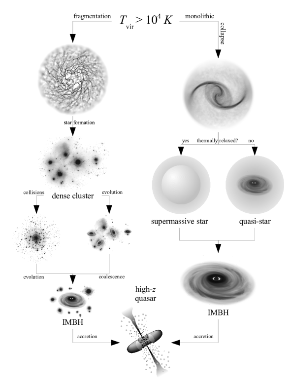
In short, the problem of creating massive BHs quickly could be resolved by any mechanism that allows massive seeds to form. Sijacki et al. (2009) found they could reproduce a BH population that fits observed properties at high- and low-redshifts by using rare seeds with masses up to about . Fig. 1.1 summarizes several possibilities that lead to intermediate-mass BHs that are massive enough to grow into SMBHs by redshift . In the next subsection, I discuss how such massive seeds can form through the monolithic gravitational collapse of massive pregalactic clouds.
1.1.3 Direct collapse
Loeb & Rasio (1994) outline a number of obstructions to the direct formation of a SMBH at the centre of a DM halo. Among them is fragmentation (see Section 1.1.1), which is principally decided by the efficient formation of molecules and their ability to cool. A further obstruction is the transport of angular momentum. If angular momentum is not transported efficiently, a large self-gravitating disc forms. If unstable to fragmentation, such an object is more likely to form a cluster of smaller objects than a single supermassive one. High-resolution simulations (Regan & Haehnelt 2009b; Wise & Abel 2007) of material in massive halos () indicate that such discs are gravitationally stable. If these discs do not fragment, does angular momentum still preclude direct collapse?
Numerical simulations have long indicated the existence of triaxial or bar instabilities in self-gravitating discs (Ostriker & Peebles 1973). Shlosman, Frank & Begelman (1989) proposed these as a mechanism for effective angular transport to feed gas to active galactic nuclei. BVR06 invoke the same mechanism in pregalactic halos. They show that, for a variety of angular momentum distributions, a reasonable number of halos are susceptible to runaway collapse through a series of bar instabilities. Indeed, Wise, Turk & Abel (2008) observe such a cascade of bar instabilities in their simulations of collapsing halos.
What is the nature of the object that forms? There are two possibilities. I shall explore their evolution in more detail in the next section and provide a simple outline of their structure here. BVR06 argue that a small protostellar core forms and continues to accrete material at a rate on the order of . Because the gas accumulates so quickly, the envelope of the star does not reach thermal equilibrium during its lifetime (Begelman 2010). After hydrogen burning is complete, runaway neutrino losses cause the core to collapse to a stellar mass BH. The structure is a then stellar mass BH embedded in and accreting from a giant-like gaseous envelope. This structure is named a quasi-star.
Alternatively, if thermal equilibrium is established throughout the protostar prior to collapse, the object resembles a metal-free star, albeit with a mass exceeding . If it is sufficiently massive, an instability from post-Newtonian terms in the equation of hydrostatic equilibrium leads to gravitational collapse before normal evolution proceeds to completion (Chandrasekhar 1964). This leads to a BH with perhaps 90 per cent of the original stellar mass (Shapiro 2004). In either case, after the stellar (or quasi-stellar) evolution ends we expect the remnant to be a massive BH (Regan & Haehnelt 2009a) that can then act as a seed for the merging and accretion processes described in the previous section.
1.2 The first luminous objects
The gradual collapse of baryonic material in the early Universe can lead to several different types of objects. Gas could fragment into metal-free stars. If the gas does not break up during the collapse, a large isolated object could form. The massive body of gas could undergo some form of stellar evolution or some fraction of it could collapse directly into a BH. In this section, I describe these various objects and their evolutions.
1.2.1 Population III stars
Metal-free stars, called Population III (Pop III) stars, have a number of properties that distinguish them from Population I and II stars. Owing to their importance in the early Universe, an extensive body of research regarding their structure and evolution now exists. I shall discuss here the aspects of metal-free stellar evolution that distinguish Pop III stars.
Based on simple theoretical arguments, Pop III stars have a top-heavy initial mass function (IMF, Bromm, Coppi & Larson 1999). That is, Pop III stars tend to have higher initial masses than metal-polluted stars. In a cloud of gas the smallest mass unstable to collapse, the Jeans mass, scales with the temperature of the gas. The strongest cooling agent in the early Universe is molecular hydrogen, which only cools effectively to . Present-day molecular clouds can cool further because of abundant molecules that include carbon, nitrogen and oxygen. This suggests that Pop III stars are on average more massive than their Pop I or II cousins. Until recently, consensus suggested Pop III stars would have masses on the order of so the literature is focused on this case (Bromm et al. 1999). Recent work (e.g. Clark et al. 2011; Hosokawa et al. 2011; Stacy et al. 2012) suggests that Pop III stars may have instead had masses on the order of because the protostellar disc fragments or evaporates before all of the material has accreted onto the central protostar.
Massive stars usually burn hydrogen into helium via the catalytic carbon-nitrogen-oxygen (CNO) cycle. In the absence of any initial carbon, nitrogen or oxygen only the proton-proton chain (pp chain) is available to slow the gradual contraction of a protostar. The pp chain scales weakly with temperature and, for such massive stars, fails to halt the contraction of the star up to core temperatures on the order of . At these temperatures, the process produces a trace amount of carbon, which is quickly converted into an equilibrium abundance of carbon, nitrogen and oxygen. The principal source of energy then shifts from the pp chain to the CNO cycle Marigo et al. 2001; Siess, Livio & Lattanzio 2002. In lower-mass stars, sufficient CNO abundances are only reached during the main sequence but, in stars with , the dominance of the CNO cycle is established earlier. For stars more massive than , the equilibrium mass abundance of carbon, oxygen and nitrogen is between about and (Bond, Arnett & Carr 1984).
These massive stars live short lives. They are radiation-dominated, so , where is the Eddington luminosity. Because the main-sequence lifetime scales as and , it follows that is roughly constant. The lifetime of a star is about (Marigo, Chiosi & Kudritzki 2003) and decreases only slightly as the mass increases. The cores are convective on the main sequence and remain so during helium burning. This commences almost immediately after hydrogen is exhausted so there is no first dredge-up. After burning helium, the core burns carbon and then contracts on dynamical timescales towards a temperature and density at which oxygen burns.
Thereafter, stars with become unstable to an electron-positron pair-production instability and they are classified as very massive objects (Bond et al. 1984). Their core temperatures are hot enough for photons to spontaneously form electron-positron pairs. This pair formation reduces the radiation pressure so the star contracts and the core temperature increases. The increase in temperature leads to more pair-production and the contraction runs away.
The pair-unstable collapse commences after core helium depletion. During the collapse, oxygen ignites explosively in the core. For stars in the range , oxygen ignition releases enough energy to completely disrupt the star in a pair-instability supernova (PISN, Fryer et al. 2001). These events present an important opportunity to pollute the early Universe with the metals produced in the first stars because the entire star’s worth of material is expelled (Heger et al. 2003).
For stars more massive than , the collapsing material is so strongly bound that even the fusion of the entire core into silicon and iron cannot halt its collapse. Most of the mass in the core is burnt to iron-group elements and the core ultimately collapses into a BH. For a star, the initial BH mass is about but it quickly accretes the remaining or so of core material (Fryer et al. 2001). For stars with masses over , about half of the star’s mass contributes to the near-immediate mass of the BH (Ohkubo et al. 2006).
Fig. 1.2 summarizes the fates of Pop III stars with masses up to . The final mass of a stellar remnant is plotted as a function of the initial mass of its progenitor according to the models of Heger & Woosley (2002). The plot includes masses below , which I have not discussed.
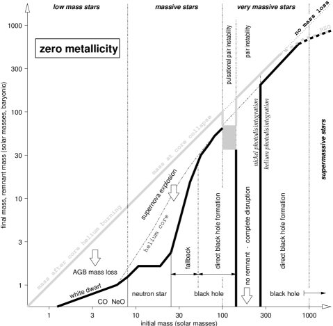
There are two notable omissions to the evolution described above. These are mass loss and rotation. Mass loss from hot stars is usually driven by atomic transition lines but these are absent in the metal-free atmospheres of Pop III stars and radiation-driven winds are very weak (Kudritzki 2002). Baraffe, Heger & Woosley (2001) and Sonoi & Umeda (2012) additionally found that mass loss via fusion-driven pulsational instabilities is typically only a few per cent. Consequently, mass-loss from the surface of Pop III stars is usually ignored (Marigo et al. 2001).
Angular momentum is imparted to primordial gas during hierarchical mergers and is preserved in its subsequent collapse. Stacy, Bromm & Loeb (2011) estimated the rotation speeds of primordial stars by following the velocities and angular momenta of gas in simulations of Pop III star formation. They found that there is enough angular momentum for the stars to be born at near break-up speeds. If the stars rotate sufficiently rapidly to shed mass from their surfaces, angular momentum is quickly lost and further rotational mass loss is limited. However, rotation can lead to additional mixing processes that bring metals to the surface and allow line-driven winds to develop. Extra mixing also extends core-burning lifetimes and modifies nucleosynthetic yields. Chatzopoulos & Wheeler (2012) calculated pre-supernova stellar models for a range of masses and rotation rates without surface mass loss and found that the minimum mass for a PISN decreases dramatically. For an initial surface rotation rate of , where is the critical Keplerian rate, the minimum mass is about .
For massive PISN progenitors (), significant rotation delays accretion by the core BH. Though the delay is not itself significant, it leads to the formation of a disc, which probably launches a jet (Fryer et al. 2001). Such a jet could experience explosive nucleosynthesis before polluting the interstellar (or even intergalactic) medium with metals. If the star is more massive than about , the jet cannot escape the stellar atmosphere. The metals would then pollute the remaining H-rich envelope but the jet itself would go unseen (Ohkubo et al. 2006).
1.2.2 Supermassive stars
Hoyle & Fowler (1963) suggested that stars with masses exceeding could explain the tremendous luminosity of quasars. Though consensus ultimately settled on quasars being accreting BHs (Salpeter 1964; Lynden-Bell 1969), these objects were modelled extensively and much of the work cited here is from that era. Only recently have supermassive stars resurfaced, now as the progenitors of high-redshift SMBHs.
The properties of very massive stars, as described in the previous subsection, hold for increasing mass until a new instability is invoked. In Newtonian gravity, stars with adiabatic index below the critical value are known to be dynamically unstable. Purely radiation-dominated stars have precisely this critical value but pure radiation is not possible because some gas is always present and raises the adiabatic index. Real radiation-dominated stars are thus stable, even if only marginally so. However, if we include the post-Newtonian terms of general relativity (GR) in the equation of hydrostatic equilibrium, the critical adiabatic index is increased to just over (Chandrasekhar 1964) and radiation-dominated stars are susceptible to the GR instability. Stars that are expected to be GR unstable are classified as supermassive stars (Appenzeller & Fricke 1971).
Because radiation pressure depends on temperature and a star’s core temperature increases over its life, stars of different masses become GR unstable during different phases of evolution. In the non-rotating case, Fricke (1973) estimated that a zero-metallicity star becomes unstable during its main-sequence life if and during its He-burning phase if . These bounds increase substantially if the star is rotating (Fricke 1974). Once the instability sets in, collapse is certain: H-ignition in a metal-free star is insufficient to stop it. Fully general-relativistic calculations (Shibata & Shapiro 2002) confirm that a BH forms with a mass of roughly 90 per cent of the star’s original mass.
A fundamental feature in the formation of a supermassive star is that hydrostatic equilibrium is established throughout the protostar. If this is not the case, the models above are not valid. Dynamical, non-homologous collapse can lead instead to a pressure-supported protostellar core accreting rapidly from the surrounding material and I describe this next.
1.2.3 Quasi-stars
One of the greater obstacles to the collapse of a single, supermassive baryonic object in the early Universe (see Section 1.1.3) is angular momentum loss (Loeb & Rasio 1994). The collisions and mergers of DM halos give them angular momentum, which is imparted to the baryonic material they contain. BVR06 outline a scenario where the angular momentum is transported via the bars-within-bars mechanism described by Shlosman et al. (1989). Whenever the ratio of rotational kinetic energy of the gas to the gravitational potential exceeds a critical factor, the disc is liable to form a bar. The bar transports angular momentum outwards and material inwards without significant entropy transport. Once the infalling material stabilizes, it cools rapidly and another bar forms. The result is a cascade of instabilities and the infall of material on dynamical timescales.
Eventually, the most central material becomes pressure-supported. The instability is then quenched because rotational support is no longer dominant. The pressure-supported object accretes at a rate on the order of and becomes radiation-dominated. BVR06 claim that infalling material creates a positive entropy gradient. This stabilises the pressure-supported region against convection. It also means that the surface layers compress the underlying material and that there is a core region of a few beneath the radiation-dominated envelope where the pressure remains gas-dominated. Both claims are supported by models of rapidly-accreting massive protostars presented by Hosokawa, Omukai & Yorke (2012), who followed the stars’ evolution up to core hydrogen ignition.
Begelman (2010) considered the evolution of the growing thermally-relaxed core. As in Pop III stars, hydrogen burning begins through pp chains but the core’s contraction continues until a trace amount of carbon is created through the process. Hydrogen subsequently burns through the CNO cycle. The hydrogen-burning phase lasts a few million years during which the core grows but does not incorporate the total mass of the object. After the core exhausts its central hydrogen supply, it contracts and heats up to many . At these temperatures, the core collapses owing to neutrino losses.
The outcome of this evolution is an initially stellar-mass BH embedded in a giant-like envelope of material. The BH quickly begins accreting from the surrounding envelope. The radiation released in the flow settles near the Eddington-limited rate of the whole object and drives convection throughout the envelope, even if it was convectively stable before core-collapse. BVR06 called this configuration a quasi-star because the envelope is star-like but the central energy source is accretion on to the BH rather than nuclear reactions.
BRA08 explored the structure of quasi-stars in some detail. The accretion on to the BH is taken to be an optically thick variant of spherical Bondi accretion (Flammang 1982) reduced by radiative feedback and the limitations of convective energy transport from the base of the envelope. The radiation-dominated envelope is convective (Loeb & Rasio 1994) and well-approximated by an polytrope. At the base of the envelope, and , so nuclear reactions can safely be ignored.
Above the convective region is a radiative atmosphere. Initially, the temperature of the radiative zone is of order for a quasi-star. As the BH and its luminosity grow, the atmosphere expands and the photospheric temperature falls. BRA08 claim that once , the entire atmosphere experiences super-Eddington luminosity. It expands more quickly, leading to faster cooling and a runaway process that disperses the photosphere. The convection zone becomes unbounded and is in effect released from the BH. The life of the quasi-star ends and leaves a BH of at least a few thousand solar masses. The models in this dissertation do not support this scenario. The BH is either stopped by reaching a fractional mass limit similar to the Schönberg–Chandrasekhar limit or it continues to accrete the whole gaseous envelope.
Angular momentum may play a role in the structure of quasi-stars. Its effect is probably minor for the envelope structure but might be significant for the BH’s immediate surroundings. The angular momentum of the accreted material leads to the formation of a disc, which decreases the accretion efficiency. The emission from the disc affects the innermost layers of the envelope and ongoing accretion affects the spin of the BH.
1.3 Outline of this dissertation
The remainder of this dissertation describes my work in six chapters. In Chapter 2, I provide the technical details of the Cambridge stars code, which was used to calculate models in Chapters 3, 4 and 6. In Chapter 3, I describe models of quasi-stars constructed after the example of BRA08 and find two main results. First, the models are highly sensitive to the location of inner boundary radius. Secondly, the models are all subject to a robust limit on the final mass of the black hole as a fraction of the total mass of the quasi-star. In Chapter 4, I confront the first problem by constructing a new set of boundary conditions and find that the evolution of the models is very different. For all parameter choices, the BHs ultimately accrete the whole envelope.
In Chapter 5, I explain the fractional mass limits found in Chapter 3. In short, the mass limit is analogous to the Schönberg–Chandrasekhar limit: the maximum fractional mass that an isothermal stellar core can achieve when embedded in a polytropic envelope with index . I extend my work to incorporate other polytropic limits discussed in the literature. The description of these limits leads to the construction of a test that determines whether a polytropic model is at a fractional mass limit. In Chapter 6, the test is applied to realistic stellar models. It appears that exceeding a fractional mass limit always occurs when a star evolves into a giant and I introduce and discuss the long-standing problem of what causes this behaviour. In Chapter 7, I summarize my research and propose directions for future work on SMBH formation and the red giant problem. {savequote}[80mm] fortran–the "infantile disorder"–, by now nearly 20 years old, is hopelessly inadequate for whatever computer application you have in mind today: it is now too clumsy, too risky, and too expensive to use. \qauthorEdsger W. Dijkstra, 1975
Chapter 2 The Cambridge stars code
A triumph of 20th century astrophysics is the development of a successful stellar model, which describes stars as spherical, static, self-gravitating fluids in local thermodynamic equilibrium. This leads to a system of non-linear differential equations that must be solved numerically. With the advent of modern computing after the second world war, an increasing number of solutions were calculated and most observable properties of stars and clusters were explained. Nowadays, these calculations are easily performed using consumer-level hardware and the theory on which they are based forms a standard body of knowledge. The reader should not infer, however, that stellar structure and evolution is wholly understood. Though the standard model is successful, it is also incomplete. There are a number of processes, including rotation and surface mass-loss, that are poorly understood and the subject of ongoing research.
In this chapter, I describe the standard equations of stellar structure and evolution and the Cambridge stars code, which solves them. The stars code was originally written by Eggleton (1971, 1972, 1973). It has subsequently been updated and modified by Han et al. (1994), Pols et al. (1995), Eldridge & Tout (2004), Stancliffe et al. (2005), Stancliffe & Glebbeek (2008) and Stancliffe & Eldridge (2009) but its distinguishing features remain unchanged. The structure, composition and distribution of solution points are calculated simultaneously using a relaxation method.
I describe here the technical details of the standard version of the code, which was used to produce the stellar models in Chapter 6. I also indicate modifications that I made to improve accuracy and convergence when modelling quasi-stars. For quantities that are variables in the parameter input file (usually data) I have given their corresponding names in the stars code in a typewriter font. e.g. (EG).
For the quasi-star models in Chapters 3 and 4, the inner boundary conditions were replaced with those of the relevant models described in each chapter. For the work described in Chapter 4, I extended a variant of the code that includes rotation (rose, Potter, Tout & Eldridge 2012) by adding corrections to the structure equations from special and general relativity devised by Thorne (1977). These extensions are described in Section 4.2.
2.1 Equations of stellar evolution
The description of a star as a spherical, static, self-gravitating fluid in local thermodynamic equilibrium leads to a system of differential equations that allows the calculation of bulk properties like temperature, density and luminosity as a function of radius in the star. These are the structure equations. They depend on the microscopic properties of the material, which must be provided either through approximate functions or as interpolations of tabulated data. These are the matter equations. Finally, the microscopic properties depend on the chemical composition of the stellar material. The gradual change in a star’s structure is caused by changes captured by the composition equations. These describe how the distribution of elements changes over time owing to redistribution through convection and transformation through fusion. In this section, I briefly review each set of equations. For complete derivations, the reader should consult any standard textbook on stellar structure. e.g. Kippenhahn & Weigert (1990).
2.1.1 Structure
The macroscopic structure of a star is described by four differential equations. The spherical approximation requires one independent variable, which must be monotonic. The usual choices are the local radial co-ordinate or the local mass co-ordinate and the differential equations are given below for both. The first three equations describe the local conservation of mass,
| (2.1) |
hydrostatic equilibrium,
| (2.2) |
and energy generation,
| (2.3) |
where is the gravitational constant, the density at , the pressure, the temperature, the luminosity and the total energy generation rate per unit mass. The total energy generation is a combination of contributions from nuclear reactions , neutrino losses and heating or cooling via contraction or expansion, referred to here as the thermal energy generation rate , where is the local specific entropy and represents time. The thermal energy generation is zero when the star is in thermal equilibrium.
The fourth structure equation describes how energy is transported through the star. In general, we write
| (2.4) |
where depends on whether energy is transported by radiation or convection. If the temperature gradient is due to radiation alone,
| (2.5) |
where is the radiation constant, the speed of light and the opacity.
If the radiative temperature gradient is greater than the adiabatic temperature gradient, at constant entropy ,a parcel of material that is displaced upward in the star becomes hotter and sparser than the material around it. In this unstable situation, the parcel floats upwards until it dissolves and releases its heat into its surroundings. Similarly, a parcel displaced downward is unstable to sink and cool material beneath it. The net result is a combination of upward and downward flows that transport heat outwards. We call this process convection. Regions in the star where are convectively unstable and energy is transported at least in part through the convective motion of material.
To calculate the convective temperature gradient, we use mixing-length theory (Böhm-Vitense 1958). Suppose that a parcel of material rises adiabatically through a radial distance , called the mixing length, before dispersing. The difference in internal energy between a parcel of gas and its surroundings is , where is the specific internal energy and the specific heat capacity at constant pressure. After rising one mixing length, the difference between the temperature of the parcel and its surroundings is
| (2.6) | ||||
| (2.7) | ||||
| (2.8) |
where we have defined the pressure scale height . The luminosity from convective heat transport is the excess heat multiplied by the amount of material that carries it, so we write
| (2.9) |
where is the convective velocity. Buoyancy accelerates the parcel at a rate , where is the local acceleration due to gravity. The blob accelerates over one mixing length so its average velocity over the journey is . Incorporating this into the convective luminosity gives
| (2.10) |
The total luminosity is given by combining the radiative and convective components. To complete the description, the mixing length must be specified. In the stars code, the mixing length is , where (ALPHA) takes a default value based on approximate calibration to a solar model.
Mixing-length theory is a crude but effective model of convection. It only considers local conditions and ignores the known asymmetry between the expansion of upward flows and the corresponding contraction of downward flows. The mixing length can even be larger than the radial extent of the convective region. In addition, the mixing length is a free parameter. The scale factor is chosen so that models agree with observations of the Sun but it is not clear that the same value of should apply to all stars or all phases of evolution. Despite these flaws, mixing-length theory works well. Near the photosphere, convection is very inefficient, so the temperature gradient takes its radiative value. In deep convective regions, such as the convective cores of massive main-sequence stars, convection is very efficient and the temperature gradient is nearly adiabatic. The more difficult intermediate case exists when convection occurs in the outer envelope as in red giants.
2.1.2 Matter
To solve the differential equations, we require three equations that describe the microscopic properties of the stellar material as a function of bulk properties and the composition. They are the opacity law , the nuclear and neutrino energy generation rates and , and an equation of state that relates the pressure, density and temperature. All three matter equations are functions of density, temperature and the elemental abundances . Simple expressions for these properties do not generally exist so they are drawn from data produced by either detailed calculations or experiments.
The opacity is computed by interpolating in a table of values. The most recent tables were compiled by Eldridge & Tout (2004). For each total metal abundance, or metallicity, , data are tabulated in a 5-dimensional grid of temperature , density parameter , hydrogen abundance , carbon abundance and oxygen abundance . The data cover from to in steps of , from to in steps of , at , , , and , and and at , , , , , , and . The tables are populated in the temperature range from to using data from the OPAL collaboration (Iglesias & Rogers 1996). At lower temperatures, data are taken from Alexander & Ferguson (1994). The low temperature tables do not include enhanced carbon and oxygen abundances so opacity changes due to changes in and are not calculated when . The high-temperature regime is filled according to Buchler & Yueh (1976). Stancliffe & Glebbeek (2008) replaced the molecular opacities for , , OH, CO, CN and with the procedure described by Marigo (2002).
If the density parameter or temperature takes a value that is not covered by the opacity table, the subroutine returns the nearest value of the opacity that is in the table. This occurred at the innermost points of the models described in Chapter 4. There, the temperature is very high, the density very low and the opacity dominated by Compton scattering. The extrapolation returns a constant opacity although, in reality, the opacity is a decreasing function of temperature. The affected region represents less than of the envelope and has little effect on the results.
Nuclear reaction rates are taken from the extensive tables of data compiled by Caughlan & Fowler (1988). Cooling rates owing to neutrino losses are drawn from those of Itoh & Kohyama (1983), Munakata et al. (1987) and Itoh et al. (1989, 1992). The reaction rates provide both the energy generated and the rate at which elements are transformed through nuclear fusion.
The quasi-star models in Chapter 3 include a substantial fraction of gas mass that is between the quasi-star envelope and the black hole. Using a temperature profile (Narayan, Igumenshchev & Abramowicz 2000), I estimated the composition changes owing to pp chains assuming complete mixing down to times the inner radius. I found no significant change to the hydrogen and helium abundances and conclude that the associated energy generation is also negligible. Although the temperatures in these regions are well over , the densities are typically only a few and decline rapidly. This is two orders of magnitude smaller than at the centre of the Sun and the objects are much shorter-lived.
The same models also neglect heat loss via neutrino emission. I estimated total neutrino loss rate using the analytic estimates of Itoh et al. (1996) and integrated them over the interior region in the fiducial run and found that the neutrino losses are at most 6 per cent of the total luminosity if the flow extends to the innermost stable circular orbit. Such losses would in effect decrease the radiative efficiency but the structure is principally determined by the convective efficiency so the envelopes remain stable against catastrophic neutrino losses.
Finally, the static structure problem is completed by specifying an equation of state (EoS). The stars code uses the EoS developed by Eggleton et al. (1973). The variable used in the program code is a parameter which is related to the electron degeneracy parameter by
| (2.11) |
In degenerate material, the pressure is calculated by approximating the Fermi–Dirac integrals as explicit functions of the parameter . The EoS package provides the pressure and density , along with derived parameters, in terms of and temperature . The ionisation states of hydrogen and helium are calculated, as is the molecular hydrogen fraction. Pols et al. (1995) described additional non-ideal corrections owing to Coulomb interactions and pressure ionization. It is presumed that all metals are completely ionized. In cool metal-free material, the electron fraction approaches zero and tends to zero too. The code refers to as an intrinsic variable, which tends to negative infinity. To avoid associated numerical errors, an insignificant minimum electron density, , was added. I compared evolutionary tracks for a star with and without this addition and found no discernible difference in the results.
Quasi-stars are strongly radiation-dominated. The EoS is very close to a simple combination of ideal gas and radiation,
| (2.12) |
where is the mass of a proton and the mean molecular weight. The ionisation state of the gas is important to determine and the detailed EoS in the stars code provides a significant improvement over previous models of quasi-stars.
2.1.3 Composition
The structural changes that occur during a star’s life are driven by changes in its chemical composition. The stars code solves for seven chemical species , , , , , , } in the structure equations. The abundances of and are presumed to be constant. The abundance of is set so that all the abundances add up to 1. Additional equilibrium isotopic abundances can be calculated explicitly after a solution for the current timestep has been found but I did not use this functionality.
Each chemical species can be created or destroyed in nuclear reactions or mixed by convection. Mixing is treated as a diffusion process which, combined with the creation and destruction through fusion, leads to an equation
| (2.13) |
for each chemical species. Here, is the fractional mass abundance of element , and are the rates at which the element is created and destroyed and is a diffusion coefficient related to the linear diffusion coefficient by . In the code, is approximated by
| (2.14) |
where (RCD) is a parameter, is the total mass and is the lifetime of the star in its current evolutionary phase (Eggleton 1972).
2.2 Boundary conditions
To solve the system of differential equations for a star, we need a set of boundary conditions. The four structure equations are first-order in the dependent variable so we require four boundary conditions. In addition, we require two equations that specify the inner and outer value of the independent variable. For each second-order composition equation, two conditions are specified by requiring no diffusion across the innermost and outermost points. We thus require six conditions. Three are applied at the surface of the star and three at the centre.
2.2.1 The surface
The surface of the star is defined where the mass co-ordinate is equal to the total mass , which is given as a parameter in the calculation. If the total mass of the star is changing because of accretion or mass loss, the total mass is simply changed over time consistently with the model that is being calculated. There is no provision for additional pressure owing to the velocity of material leaving from or arriving at the surface. The total luminosity is specified by assuming that the star radiates into a vacuum as a black body, which gives
| (2.15) |
where is the radius of the surface, the Stefan–Boltzmann constant and the effective temperature. The gas pressure at the surface is given by
| (2.16) |
where is the Eddington luminosity. At the Eddington luminosity, radiation pressure alone would balance gravity. If the luminosity were greater, the force of radiation would accelerate material away from the star.
2.2.2 The centre
At the centre of the star, the formal boundary conditions are but these lead to divergences in the differential equations. The central point of the model is calculated as an average of the formal boundary conditions and the values at the first point from the centre. For a specified innermost mass , the central radius is defined by
| (2.17) |
and the central luminosity by
| (2.18) |
Quasi-stars are modelled with the stars code by choosing new boundary conditions for the innermost point. For example, the inner mass is at least the central black hole mass. Because the new inner boundaries take finite values, I omit the averaging process used to avoid singularities at the centre. The innermost meshpoint is computed directly on the specified boundary. Different boundary conditions were used for the models described in Chapters 3 and 4 so detailed discussions of the boundary conditions in each set of models are deferred to Sections 3.1 and 4.1.
2.3 Implementation
The structure, matter and composition equations define the mathematical problem of calculating the structure and evolution of a star. To calculate solutions numerically, the variables are determined at a finite number of meshpoints. The quasi-star models described in Chapters 3 and 4 all have 399 meshpoints; the stellar models of Chapter 6 have 199. The structure equations are transformed into difference equations that are corrected iteratively until the sum of the moduli of the corrections is smaller than a user-specified tolerance parameter (EPS). The tolerance parameter is throughout this dissertation. Once a satisfactory solution is reached, the model is evolved forward by one timestep and a new solution is computed. The time evolution is fully implicit so that the changes in the time derivatives are computed self-consistently with the structure.
2.3.1 Mesh-spacing
The independent variable in the structure equations can be any monotonic variable in the star. The stars code uses the meshpoint number distributed such that a function is equally spaced on the mesh. In other words, we introduce an equation , where is an eigenvalue. The function , called the mesh-spacing function, can depend on any of the variables in the model provided that it remains monotonic in and has analytic derivatives with respect to the variables. By choosing a function that varies rapidly in regions where greater numerical accuracy is required, we focus the meshpoints automatically on these regions of interest.
The present version of the stars code uses a mesh-spacing function
| (2.19) |
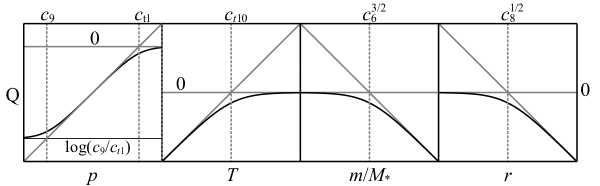
The default parameters are specified in table 2.1111The labels of the parameters have been chosen to match the variables used in the code. and the qualitative forms of the second, fourth, fifth and sixth terms are shown in Fig. 2.1. Points are concentrated towards where the gradient of is larger. Each term is chosen so that points are either concentrated towards regions that require additional resolution or distributed away from regions that do not. The default values for the parameters gave satisfactory results and were used in all models in this dissertation.
The main contributor the the mesh-spacing is the fifth term, which distributes points like but reduces resolution at the centre. The first term spreads points evenly in the pressure co-ordinate. The second and third terms allow points to be concentrated within the pressure ranges defined by and and between and . When the parameters have their default values, is so large that the denominator under the logarithm can be ignored as a constant and the third term is ignored (i.e. ). The fourth term concentrates points towards the upper atmosphere, where and extra resolution is required to properly resolve the hydrogen ionization zones. The sixth term weakly moves points toward regions with .
| C(1) | C(2) | C(3) | C(4) | C(5) | C(6) |
| C(7) | C(8) | C(9) | C(10) | CT1 | CT10 |
2.3.2 Difference equations
Each differential equation containing a spatial derivative is recast as a difference between values at two neighbouring points, denoted by subscript and . Averages between two neighbouring points are denoted by subscript . The distribution of points in the mesh is solved through
| (2.20) |
The structure equations for mass conservation, hydrostatic equilibrium and energy generation become
| (2.21) | |||
| (2.22) |
and
| (2.23) |
The energy transport equation is
| (2.24) |
The composition equations become
| (2.25) |
where I have used the ramp function, , and is the abundance of element at the previous timestep. The boundary conditions for the composition equations are in effect as appropriate. Note that the simultaneous evaluation of the structure, composition and non-Lagrangian mesh is a defining feature of the Cambridge stars code.
2.3.3 Solution and timestep
The system of difference equations and their boundary conditions is solved by a relaxation method (Henyey et al. 1959). Given an initial approximate solution, the variables are varied by a small amount (DH0) to determine derivatives of the equations with respect to the variables. The matrix of these derivatives is inverted to find a better solution. This process is iterated through a Newton–Rhapson root-finding algorithm until the sum of corrections to the solution is smaller than some parameter (EPS). The solution is then recorded and the next model in time is computed by the same process.
The timestep is calculated by comparing the sum of fractional changes in each variable at each point with an input parameter (DDD). The next timestep is chosen so that the two numbers are equal but the timestep can only be rescaled within a user-specified range (DT1, DT2). If the relaxation method fails to converge on a sufficiently accurate model, the previous model is abandoned, the code restores the anteprevious model and the timestep is reduced by a factor . I appended code so that if a value of NaN (not a number) is encountered during the convergence tests, the run is immediately aborted.
The stars code is versatile and adaptable. Its mesh-spacing function allows it to rapidly model many phases of stellar evolution without interruption and the concise source code (less than 3000 lines of fortran) makes modification straightforward. In the next two chapters, I modify the central boundary conditions to model quasi-stars with accurate microphysics. {savequote}[80mm] We know that for a long time everything we do will be nothing more than the jumping off point for those who have the advantage of already being aware of our ultimate results. \qauthorNorbert Wiener, 1956
Chapter 3 Bondi-type quasi-stars
In this chapter, I present models of quasi-star envelopes where the inner black hole (BH) accretes from a spherically symmetric flow. The accretion flow is based on the canonical model of Bondi (1952) and these quasi-star models are referred to as Bondi-type quasi-stars in later chapters. Begelman, Rossi & Armitage (2008, hereinafter BRA08) studied these structures using analytic estimates and basic numerical results. I model the envelope using the Cambridge stars code, which accurately computes the opacity and ionization state of the envelope. In Section 3.1, I describe the boundary conditions used in this chapter. The results of a fiducial run are presented and discussed in Section 3.2 and further runs with varied parameters are described in Section 3.3. In Section 3.4, the stars models are compared with the results of BRA08.
The models in this chapter lead to two main results that are explored further in subsequent chapters. First, for a given inner radius, the models stop evolving once the BH reaches just over one-tenth of the total mass of the quasi-star regardless of the total mass of the system or the radiative efficiency of the accretion flow. Polytropic models of quasi-star envelopes exhibit the same robust fractional limit on the BH mass and the mechanism that causes the maximum is thus a feature of mass conservation and hydrostatic equilibrium. In Chapter 5, I show that the BH mass limit found below is related to the Schönberg–Chandrasekhar limit and, in Chapter 6, I consider some consequences for the evolution of giant stars.
Secondly, the models are strongly sensitive to the inner boundary radius. Roughly speaking, the final mass of the BH is inversely proportional to the inner radius. While the boundary conditions used here are reasonable, the models they produce are unreliable even though the qualitative evolution may be realistic. In the next chapter, I address this by constructing models with a different set of boundary conditions and find that the evolution is qualitatively very different from what is described in this one.
3.1 Boundary conditions
Stellar evolution codes normally solve for the interior boundary conditions , where is the radial co-ordinate, is the mass within a radius and is the luminosity through the sphere of radius . To model quasi-stars, these boundary conditions are replaced with a prescription for the BH’s interaction with the surrounding gas as described below. Loeb & Rasio (1994) showed that a radiation-dominated fluid in hydrostatic equilibrium and not generating energy must become convective so the quasi-star envelope should be approximated by a gas with polytropic index . This presumption is used below but in the subsequent calculations the adiabatic index ( at constant entropy, where is the pressure and the density) is determined self-consistently by the equation-of-state module in the code.
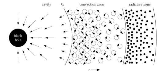
Fig. 3.1 shows the basic components of the model adopted in this chapter. The inner radius is a fixed multiple of the Bondi radius, inside which material falls on to the central BH. A substantial amount of mass can be found inside this cavity and its mass is included in the inner mass boundary condition. The stars code models the hydrostatic envelope outside the inner radius. Near , the envelope is convective but it is necessarily radiative at the surface because of the surface boundary conditions. Although not included in the diagram, additional intermediate radiative zones can exist (see Fig. 3.3).
3.1.1 Radius
The radius of the inner boundary of the envelope should be the point at which some presumption of the code breaks down. Following BRA08, I choose the Bondi radius , at which the thermal energy of the fluid particles equals their gravitational potential energy with respect to the BH. By definition,
| (3.1) |
so
| (3.2) |
where is the mass of a test particle, the adiabatic sound speed, the mass of the BH and Newton’s gravitational constant.
BRA08 used the inner boundary condition
| (3.3) |
We therefore implement the radial boundary condition
| (3.4) |
where is a parameter that varies the inner radius. Larger values of correspond to smaller inner radii and therefore a stronger gravitational binding energy there. Our main results use whereas the boundary condition used by BRA08 corresponds to .
3.1.2 Mass
For the mass boundary condition, consider the mass of the gas inside the cavity defined by the Bondi radius (equation 3.2). By definition,
| (3.5) |
where is the Schwarzschild radius. Using a general relativistic form of the equation introduces terms of order (Thorne & Żytkow 1977), which I ignore because all our models have .
To determine the mass of gas inside the cavity, we must assume a density profile of the material there because the code does not model this region. The envelope is supported by radiation pressure and is expected to radiate near the Eddington limit for the entire quasi-star. This is much greater than the same limit for the BH alone. The excess flux drives bulk convective motions. The radial density profile of the accretion flow then depends on whether angular momentum is transported outward or inward. In the former case, the radial density profile is proportional to whereas, in the latter case, it is proportional to (Narayan, Igumenshchev & Abramowicz 2000; Quataert & Gruzinov 2000). We presume that the viscosity owing to small scale magnetic fields is sufficiently large to transport angular momentum outwards even if convection transports it inwards and thus take . In Section 3.3.2, I construct a model presuming that and find that this change to the density profile inside the cavity has little effect.
Given the density at the inner boundary, the density profile must be
| (3.6) |
Evaluating equation (3.5), presuming , we obtain
| (3.7) |
The cavity mass can be estimated as follows. In a radiation-dominated polytrope, the pressure and density are related by
| (3.8) |
(Eddington 1918), where is Boltzmann’s constant, the mean molecular weight of the gas, the mass of a hydrogen atom and the ratio of gas pressure to total pressure. Taking the adiabatic sound speed to be , evaluating the Bondi radius using equation (3.2) and substituting into equation (3.7), we obtain
| (3.9) |
Fowler (1964) gives , where is the total mass of the object. For a totally ionized mixture of 70 per cent hydrogen and 30 per cent helium by mass, , so for a quasi-star of total mass , as in the fiducial result, when . The cavity mass must be included in the mass boundary condition so I use
| (3.10) |
where is given by equation (3.7).
3.1.3 Luminosity
The luminosity is determined by the mass accretion rate through the relationship
| (3.11) |
where is the speed of light, the rate of mass flow across the base of the envelope and the radiative efficiency, the fraction of accreted rest mass that is released as energy. This fraction is lost from the system as radiation so the total mass of the quasi-star decreases over time. The rate of accretion on to the BH is . i.e. the amount of infalling matter less the radiated energy. The luminosity condition is related to the BH accretion by
| (3.12) |
It is thus implicitly assumed that material travels from the base of the envelope to the event horizon within one timestep. The material actually falls inward on a dynamical timescale so this condition is already implied by the presumption of hydrostatic equilibrium.
To specify the accretion rate, we begin with the adiabatic Bondi accretion rate (Bondi 1952),
| (3.13) |
where is a factor that depends on the adiabatic index as described by equation (18) of Bondi (1952). When , . Almost all of this flux is carried away from the BH by convection. The convective flux is on the order of , where is the convective velocity, the mixing length and the specific internal energy of the gas (Owocki 2003). The convective velocity is at most equal to the adiabatic sound speed because if material travelled faster it would presumably rapidly dissipate its energy in shocks. The mixing length is on the order of the pressure scale height and the specific internal energy gradient is roughly . The maximum convective flux is therefore on the order of so the maximum luminosity is
| (3.14) |
In order to limit the luminosity to the convective maximum, the accretion rate is reduced by a factor . I therefore assume that the actual convective flux is some fraction of the maximum computed above and implement the mass accretion rate
| (3.15) |
where is the convective efficiency. In the fiducial run, .
3.2 Fiducial model
I begin the exposition of the results by selecting a run that demonstrates the qualitative features of a model quasi-star’s structure and evolution. Thereafter, I vary some of the parameters to explore how the behaviour is affected by such changes. The results presented in this section describe a model quasi-star with initial total mass (BH, cavity gas and envelope) , initial BH mass and a uniform composition of 0.7 hydrogen and 0.3 helium by mass. The envelope is allowed to relax to thermal equilibrium before the BH begins accreting.
3.2.1 Structure
| / | / | / | / | / | / | ||||
|---|---|---|---|---|---|---|---|---|---|
| 0.00 | 5 | 2.14 | 0 | .00 | 40 | .3 | 0 | .0171 | |
| 0.51 | 100 | 1.79 | 3 | .80 | 3 | .55 | 3 | .66 | |
| 1.03 | 200 | 2.08 | 25 | .3 | 2 | .23 | 11 | .1 | |
| 2.23 | 500 | 2.96 | 242 | 1 | .33 | 41 | .3 | ||
| 3.70 | 1000 | 3.70 | 1380 | 0 | .88 | 115 | |||
| 4.22 | 1194 | 3.56 | 3311 | 0 | .71 | 184 | |||
| / | / | / | / | ||||||
| 0.00 | 5 | 3.48 | 14 | .1 | 0 | .312 | |||
| 0.51 | 100 | 2.92 | 5 | .22 | 2 | .09 | |||
| 1.03 | 200 | 3.40 | 4 | .77 | 2 | .70 | |||
| 2.23 | 500 | 4.84 | 4 | .55 | 3 | .54 | |||
| 3.70 | 1000 | 6.06 | 4 | .49 | 4 | .08 | |||
| 4.22 | 1194 | 5.83 | 4 | .51 | 3 | .96 | |||
In the model, the luminosity is approximately equal to the Eddington luminosity at the boundary of the innermost convective layer. The accretion rate varies between about and as the convective boundary moves. The details of the variation are described in Section 3.2.2. A corollary of the self-limiting behaviour is that the only major effect of changing the material composition is to change its opacity and therefore the Eddington limit. The accretion rate changes but the structure is almost entirely unaffected. In the convective regions, the envelope has an adiabatic index of about (corresponding to a polytropic index ) confirming that the envelope is approximated by an polytrope. The boundaries of the convective regions depend on the ionization state of the gas but, for most of the evolution, all but the outermost few are convective.
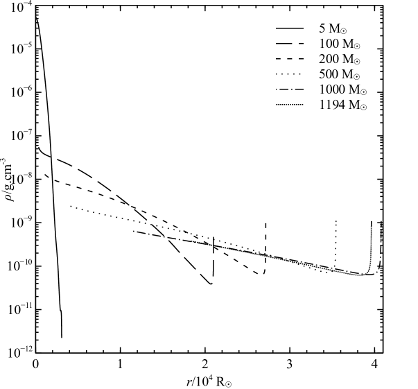
Fig. 3.2 shows a sequence of density profiles of the envelope when , , , , and . Further parameters are listed in Table 3.2. These profiles demonstrate two features of the envelope structure. First, the centre is condensed as can be seen from the rise in the density at the innermost radii. This is clearer for smaller BH masses. It is caused by the lack of pressure support at the inner boundary. To maintain hydrostatic equilibrium, the equations require
| (3.16) |
at the inner boundary so the pressure gradient steepens and the density gradient follows. Huntley & Saslaw (1975) called such structures loaded polytropes.
Secondly, the density in the outer layers is usually inverted as in all but the first density profile in Fig. 3.2. The density inversion appears once the photospheric temperature drops below about . Thereafter, the surface opacity increases owing to hydrogen recombination, the Eddington luminosity falls and the quasi-star’s luminosity apparently exceeds the limit. Density inversions are possible when the temperature gradient becomes strongly superadiabatic (Langer 1997), as is the case in regions where convection occurs but is inefficient. As an additional check, we calculated the volume-weighted average of and found it to be positive, indicating dynamical (but not pulsational) stability (Cox & Giuli 1968, p. 1057).
3.2.2 Evolution
The sequence of density profiles in Fig. 3.2 shows the interior density decreasing over time. If we consider equation (3.15), ignoring constants and using , then
| (3.17) |
The accretion rate never increases faster than so for any reasonable adiabatic index (), decreases at the inner boundary. Initially, the density decreases rapidly and the envelope expands owing to the hydrogen opacity peak at the surface. The expansion or contraction of the surface is at most about , which is five orders of magnitude smaller than the free-fall velocity. The models are thus still in hydrostatic equilibrium.
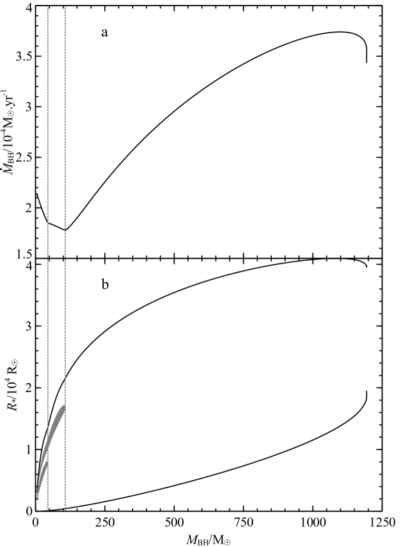
Fig. 3.3a shows the accretion rate on to the BH as a function of its mass. Fig. 3.3b shows the locations of convective boundaries as a function of BH mass and demonstrates how the rapid changes of the BH accretion rate while coincide with the disappearance of radiative regions owing to the decreasing density throughout the envelope.
Before the end of the evolution the accretion rate achieves a local maximum. At the same time, the photospheric temperature reaches a local minimum and the envelope radius a maximum (see Fig. 3.3b). We do not have a simple explanation for this but believe it is related to the increasing mass and radius of the inner cavity. Whereas a giant expands owing to contraction of the core, the inner part of the quasi-star is in effect expanding so the envelope is evolving like a giant in reverse. Initially, the expansion of the inner radius is greater than the relative contraction of the surface but the situation reverses when the surface radius reaches its maximum.
3.2.3 Inner mass limit
In the fiducial run, evolution beyond the final BH mass of is impossible. The code reduces the timestep below the dynamical timescale indicating that we cannot construct further models that satisfy the structure equations. The non-existence of further solutions can be demonstrated by constructing polytropic models of quasi-star envelopes as follows. A complete derivation of the Lane–Emden equation and an analysis of its homology-invariant form is provided in Appendix A but the relevant details are reproduced below.
Consider the equations of hydrostatic equilibrium and mass conservation truncated at some radius and loaded with some mass interior to that point. The equations are
| (3.18) |
and
| (3.19) |
with central boundary condition , where and are fixed. We scale the pressure and density using the usual polytropic assumptions
| (3.20) |
and
| (3.21) |
We define the dimensionless radius by
| (3.22) |
where
| (3.23) |
We scale the mass interior to a sphere of radius by defining
| (3.24) |
The non-dimensional form of the equations is then
| (3.25) |
and
| (3.26) |
with boundary conditions and (where, by definition, ).111If one takes , differentiates equation (3.25) and substitutes for using equation (3.26), one arrives at the usual Lane–Emden equation.
The dimensionless BH mass is expressed in terms of the inner radius by rescaling equation (3.2) as follows.
| (3.27) | ||||
| (3.28) | ||||
| (3.29) | ||||
| (3.30) |
Similarly, from equation (3.7), is expressed by
| (3.31) |
The dimensionless mass and radius boundary conditions are now related by
| (3.32) |
Thus, for a given polytropic index , we can choose a value and integrate the equations.
I integrated a sequence of solutions for and found that there exists a maximum value of , where is the total dimensionless mass of the quasi-star. The maximum occurs when . Similar limits appear for polytropic indices between and . For , the maximum is when and for the maximum is at . Fig. 3.4 shows plots of the curves of the ratio of inner to outer envelope radius ( in dimensionless variables, where is the outer radius of the envelope) against the fractional BH mass ( in dimensionless variables) for , and together with our results for the fiducial model. The maximum mass ratio is clear in each curve. In principle, further hydrostatic solutions exist along the sequence computed by stars but they require that the BH mass decreases.222I tried to compute hydrostatic solutions on the other side of the maximum mass ratio but never succeeded.
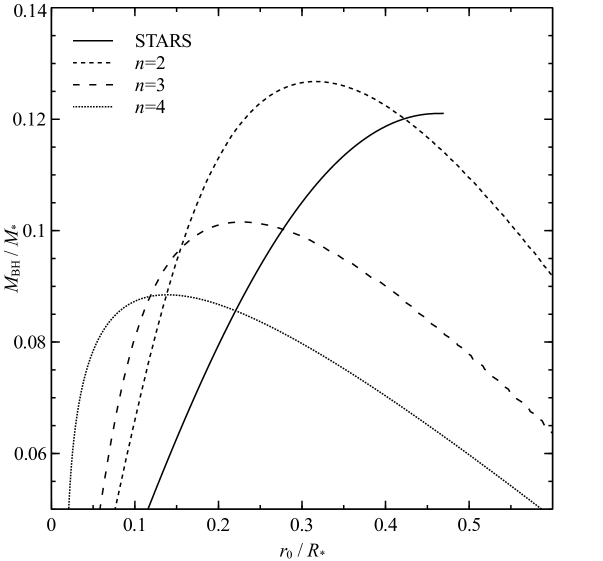
The existence of a maximum inner mass ratio is therefore a robust feature of the structure equations. Maximum ratios exist for all choices of inner radius and cavity mass in this chapter. In particular, a maximum also exists when the cavity mass is ignored completely. The cause of the maximum mass ratio is not generally clear but in Chapter 5 we show that, without the cavity gas, the maximum exists for the same reason as the Schönberg–Chandrasekhar limit. The cavity gas modifies the inner boundary condition, and therefore the envelope solution, but the same mechanism is at work.
3.2.4 Post-quasi-star evolution
At the end of the fiducial run the cavity contains . Under our assumptions, some of this material is already moving towards the BH and may become part of it. If the BH accretes all the mass in the cavity, its final mass would be , nearly half of the total mass of the original quasi-star. Presuming the BH accretes at its Eddington-limited rate, this growth would take about .
What actually happens to the material in the cavity after the end of the hydrostatic evolution? It appears that the entire envelope might be swallowed but it is not certain that this should be the case. The accretion flow is at least partly convective so there must be a combination of inward and outward flowing material within the Bondi radius. In the theoretical limit for a purely convective flow, the accretion rate is zero (Quataert & Gruzinov 2000) and half of the material is moving inward and half outward. If the flow is sustained, we might expect at least half of the cavity mass to be accreted. On the other hand the flow structure might change completely. The infalling material could settle into a disc and drive disc winds or jets so that the overall gain in mass is relatively small. Hydrostatic equilibrium is probably failing in the envelope so its dynamics might also change drastically.
Johnson et al. (2011) modelled the accretion on to massive BHs formed through direct collapse. They assumed that the BH accretes from a multi-colour black-body disc after its quasi-star phase and found that, once the BH mass exceeds about , the accretion rate decreases owing to radiative feedback. This result supports the case for a substantial decrease in the BH growth rate if a thin disc forms after the quasi-star phase but additional growth can occur during the transition to a new structure.
3.3 Parameter exploration
In Section 3.2, I established the basic qualitative structure and evolution of the quasi-star envelope. In this section, I explore their dependence on some of the parameters of the model. I begin in Section 3.3.1 with the radiative and convective efficiencies and . I then vary the choice of cavity mass in Section 3.3.2, surface mass loss and gain in Section 3.3.3 and the total initial envelope mass in Section 3.3.4. Finally, in Section 3.3.5 I vary the inner radius.
3.3.1 Radiative and convective efficiencies
Fig. 3.5 shows the accretion history against BH mass for a number of choices of radiative efficiency and convective efficiency . Because the luminosity always settles on the same convection-limited rate, a change in only rescales the accretion rate through equation (3.11) and does not affect the structure. The final BH mass and intermediate properties are the same. The only difference is that the evolution takes longer for larger values of .
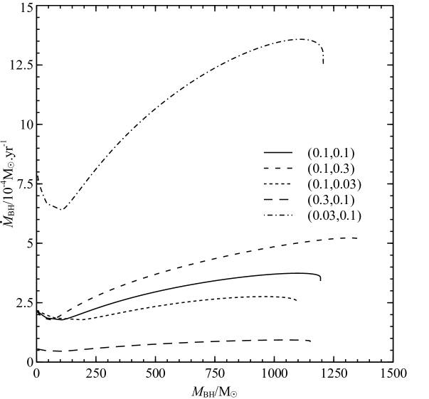
A larger convective efficiency allows a greater flux to be radiated by the accretion flow and therefore a larger accretion rate for given interior conditions. To establish the same overall luminosity, the envelope must be less dense so the discontinuities in the gradient of the accretion rate appear later. In addition, the lower density means that, although the final total inner masses are similar, the cavity mass is smaller and the BH mass larger. Conversely, for smaller values of , the envelope is denser, the discontinuities appear earlier and the final BH mass is smaller.
3.3.2 Cavity properties

If the inward transport of angular momentum by advection and convection is greater than the outward transport by magnetic fields and other sources of viscosity, the density profile in the cavity tends towards (Quataert & Gruzinov 2000; Narayan et al. 2000). Recomputing the cavity mass from equation (3.5), we find
| (3.33) |
The corresponding quasi-star evolution is shown in Fig. 3.6. The smaller interior mass leads to a less evident density spike at all times. The decreased interior mass is subject to a lower mass limit for the BH and leaves a BH of . Although the change to the cavity properties affects the numerical results, there is no qualitative change to the quasi-star evolution, which still terminates owing to the same physical mechanism as the fiducial run.
The maximum mass ratio is not principally caused by the cavity mass. Fig. 3.6 also shows a run with . The BH achieves a final mass of . A maximum mass ratio still exists, though with a different numerical value, and a similar limit is found for polytropic models with no cavity mass. In this case, the maximum mass ratio exists for the same reason as the Schönberg–Chandrasekhar limit. The connection between the mass limits is demonstrated in Chapter 5.
3.3.3 Envelope mass loss and gain
To illustrate the effect of net accretion on to the surface of the envelope, Fig. 3.6 shows the evolution of the fiducial run if the envelope accretes at a constant rate of . Although this rate initially exceeds the quasi-star’s Eddington limit, such rapid infall is believed to occur as long as the bars-within-bars mechanism transports material towards the centre of the pregalactic cloud. Accreted mass is added to the surface mass co-ordinate and no additions are made to any other equations. In particular, we do not include a ram pressure at the surface.
The only qualitative change to the evolution is that it takes longer than if the total mass had been kept constant at the same final value of . The final BH mass is subject to the same ratio limit and the larger final envelope permits a larger final BH mass of .
To investigate the effect of mass loss we use a Reimers rate (Reimers 1975), an empirical relation that describes mass loss in red giants. The mass-loss rate is
| (3.34) |
Fig. 3.6 shows the evolution for a quasi-star envelope with this prescription. The mass loss is significant but, again, there is no qualitative change in the results. The limit holds and the BH has a smaller mass of . This is in proportion with the decrease in the total mass of the quasi-star to .
3.3.4 Initial envelope mass
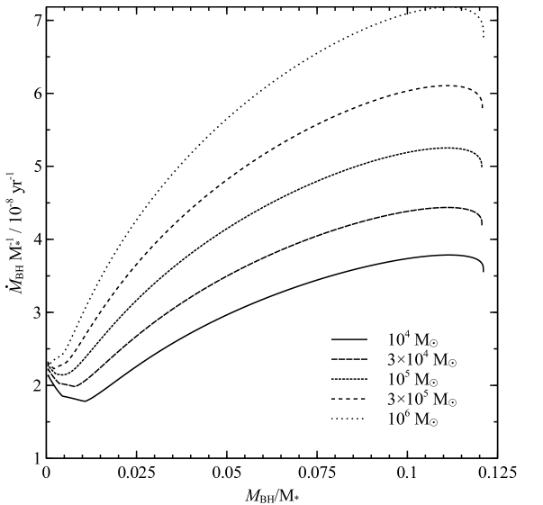
The structure of the envelope appears to be chiefly dependent on the ratio of envelope mass to BH mass. Fig. 3.7 shows the evolution of the the BH mass and of the accretion rate divided by total mass for quasi-stars of total initial masses and . The fractional upper BH mass limit holds for all the quasi-star masses in this range though the BH-envelope mass ratio after which the entire envelope is convective depends on the envelope mass.
For a given mass ratio, once the entire envelope has become convective, the following approximate relations hold for the properties of two quasi-stars of different masses (denoted by subscripts 1 and 2).
| (3.35) |
| (3.36) | |||
| (3.37) | |||
| (3.38) |
and
| (3.39) |
For example, compared with a quasi-star of mass at the same BH-envelope mass ratio, a quasi-star roughly has an interior temperature that is times smaller, a surface temperature that is times greater, an outer radius that is times greater, an interior density that is times smaller and a mass accretion rate that is times greater. Equations (3.35) and (3.36) imply that the temperature profiles of the envelopes depend almost exclusively on the BH-envelope mass ratio. The variation in inner or surface temperature, for a given mass ratio, with respect to the total mass of the quasi-star is less than 0.1 per factor of ten in the total mass. The density and radius profiles are more strongly dependent on the mass of the envelope.
The final relation (equation 3.39) implies that the lifetime of a quasi-star scales roughly as so larger quasi-stars have slightly shorter hydrostatic lifetimes. By fitting a straight line to the – relation for the five models described here, we find
| (3.40) |
Note that here denotes the initial mass of the quasi-star. In all other relations decreases slowly during the quasi-star’s evolution owing to the mass-energy lost as radiation in the accretion flow.
3.3.5 Inner boundary radius
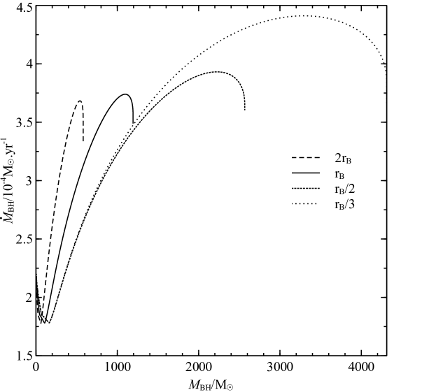
Fig. 3.8 shows the evolution of quasi-stars where the inner radius was changed to a third, half and twice the Bondi radius through the parameter . The final BH mass is strongly affected although the evolution is qualitatively similar. The results of our polytropic analysis are affected in a consistent manner. I further found that I could not construct model envelopes with and that this is reflected in the polytropic models. Although reasonable, our choice of inner radius is somewhat arbitrary and critical in deciding the quantitative evolution of the BH.
Despite this, the total mass inside the cavity is broadly similar across the models. For models with , , and , the total inner masses (BH and cavity) are approximately , , and .333The last figure is interpolated from the model profiles, which were not recorded near the last model before convergence began to fail. If the BH ultimately accretes most of the material in the cavity after its quasi-star phase ends, it reaches a similar mass for any choice of .
Begelman (2010, private communication) pointed out that, in the presence of a substantial mass of gas in the cavity, the Bondi radius should be defined for the total mass inside , not just the BH mass. Presuming the gas has a density distribution inside the cavity, this gives the equation
| (3.41) |
For an polytrope, we can substitute for dimensionless variables (see Section 3.2.3) to obtain
| (3.42) |
which only has a real positive root if . For maximum , the ratio of BH mass to total mass is for and for it is .
3.4 Comparison with Begelman et al. (2008)
BRA08 estimated some envelope properties by presuming that the envelope is described by an polytrope. They employed an overall accretion efficiency parameter444This should not be confused with defined in Section 3.2.3. , which is determined by numerical factors in the accretion rate including the radiative efficiency, convective efficiency and adiabatic index. I calibrated through the BH luminosity (equation 3 of BRA08) and chose for the fiducial run. The analytical BH luminosity is then accurate to within 0.2 per cent over the entire evolution. I also compared a run with by using , which is similarly accurate to within 0.3 per cent.
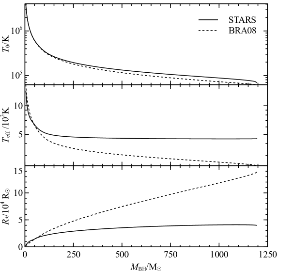

BRA08 provide the following analytic estimates for the inner temperature, photospheric temperature and envelope radius (equations 7, 11 and 10 in their paper, respectively).
| (3.43) | |||
| (3.44) |
and
| (3.45) |
Here, is the Eddington luminosity. BRA08 computed this using the opacity at the boundary of the convective zone but such estimates differ by a factor of the order of when compared with our results. The comparison is thus made using the Eddington limit with opacity .
The three estimates are plotted against the fiducial run in Fig. 3.9. The estimate for the interior temperature is accurate to within 20 per cent. The deviation grows as the approximation of the envelope to an polytrope becomes increasingly poor. The estimate for the photospheric temperature is not accurate. At the end of the run the estimated photospheric temperature is about compared with the model result of about . Because the BH luminosity estimate is accurate, it follows that the envelope radius is not because the surface luminosity is . This is confirmed in the bottom panel of Fig. 3.9. BRA08 used an inner boundary with so the analytic estimates are compared with such a run in Fig. 3.10. The interior temperature estimate is worse but the photospheric temperature estimate is better. The final surface temperature remains remains underpredicted and the surface radius inaccurate.
The analytic estimates by BRA08 can be compared with the scaling relations found in Section 3.3.4. By fixing and , equations (3.43), (3.44) and (3.45) can be re-arranged to give
| (3.46) | |||
| (3.47) |
and
| (3.48) |
These compare reasonably with the scaling relations derived from the stars models. Written similarly as power-laws in , equations 3.35, 3.36 and 3.37 have indices , and , respectively.
BRA08 argue that quasi-star evolution terminates owing to the opacity at the edge of the convection zone increasing. An increased opacity causes the envelope to expand and the opacity increases further. The envelope then expands even more and the process is claimed to run away. BRA08 refer to this process as the opacity crisis. Our results do not terminate for this reason. Similar behaviour does occur at the beginning of the evolution while the photospheric temperature is greater than but it does not disperse the quasi-star. For most of a quasi-star’s evolution, the opacity at the convective boundary is already beyond the H-ionization peak and is decreasing as the BH grows.
Instead, my models terminate because of a basic property of mass conservation and hydrostatic equilibrium. I have shown that further models do not exist in the sequence by showing that the same fractional mass limit exists in polytropic models. Direct calculation of the polytropic mass limits shows that they are similar to the results found with the stars code. In Chapter 5, I show how the fractional mass limit found here for quasi-stars is directly related to the Schönberg–Chandrasekhar limit as well as several related limits in the literature.
3.5 Conclusion
The models presented in this chapter provide several important results. The first is the existence of a robust upper limit on the ratio of inner BH mass to the total quasi-star mass, equal to about . The limit is reflected in solutions of the Lane–Emden equation, modified for the presence of a point mass interior to some specific boundaries. All the evolutionary runs here terminate once the limit is reached and it is difficult to say what happens after the hydrostatic evolution ends. Some of the material within the Bondi radius has begun accelerating towards the BH so we expect that it can be captured by the BH. The remaining material may be accreted or expelled, depending on the liberation of energy from the material that does fall inwards. After the BH has evolved through the quasi-star phase, it is probably limited to accrete at less than the Eddington rate for the BH alone and thus much less than the accretion rate during the quasi-star phase.
These results suggest that quasi-stars produce BHs that are on the order of at least of the mass of the quasi-star and around if all the material within the inner radius is accreted. For conservative parameters, this growth occurs within a few million years after the BH initially forms. Realistic variations in the parameters (e.g. larger initial mass, lower radiative efficiency) lead to shorter lifetimes. Such BHs could easily reach masses in excess of early enough in the Universe to power high-redshift quasars.
However, it is also clear that the models are critically sensitive to the choice of inner boundary radius and the results should be treated with due caution. While the Bondi radius used here is reasonable, it is worthwhile to consider other sets of boundary conditions. In the next chapter, I construct models that use a qualitatively different set of boundary conditions, which lead to very different quasi-stars than the Bondi-type models. {savequote}[80mm] With four parameters I can fit an elephant, and with five I can make him wiggle his trunk. \qauthorJohn von Neumann, attrib.
Chapter 4 CDAF-ADAF quasi-stars
In the work reported in Chapter 3, the structure of quasi-stars is calculated under the assumption that the dynamics in the cavity around the black hole (BH) are described by Bondi accretion. Although the corresponding models are reasonable and self-consistent, they are strongly sensitive to the choice of the inner radius. In this chapter, I construct models with a different set of boundary conditions and find that the corresponding models evolve very differently.
The model of the accretion flow, described in Section 4.1, depends critically on the presence of rotation in the envelope. The inner boundary of the envelope becomes sufficiently small that relativistic effects cannot be ignored as they were in Chapter 3. In Section 4.2.1, I introduce rose, a variant of the stars code that incorporates rotation in the structure equations. In Section 4.2.2, I describe additional relativistic corrections I added to the code based on the work of Thorne (1977).
In Section 4.3, I present a fiducial set of results that demonstrate the main qualitative features of the evolution of the models. The most important result is that the BH ultimately accretes nearly the whole envelope. This is in stark contrast with the results for the Bondi-type quasi-stars of Chapter 3, where the BH was subject to a robust fractional mass limit. In addition, the accretion rates in the models presented here are about an order of magnitude greater. I vary the free parameters of the model in Section 4.4 and find that the evolution remains qualitatively similar to the fiducial run. There are, however, selections of parameters for which the evolution can only be modelled if we begin with larger BH cores. Finally, there are also parameters for which so much energy is trapped in the accretion flow that the envelope cannot be supported and the initial models fail to converge.
4.1 The convective-advective boundary
Accretion on to a black hole admits solutions in which a substantial fraction of energy is trapped in the infalling gas and never radiated away. The advection of energy across the event horizon is possible when the material is so optically thick that radiation takes too long to scatter out through the gas or the gas is so sparse that radiation is inefficient. The loss of energy to the BH permits advection-dominated accretion flows (ADAFs, Narayan & Yi 1994), which are unique to BHs (see Narayan & McClintock 2008, for a review).
It is understood that these flows are convectively unstable in the radial direction. Narayan, Igumenshchev & Abramowicz (2000) and Quataert & Gruzinov (2000) independently found self-similar accretion flows with convection where the outward transport of angular momentum by viscosity is precisely balanced by the inward transport by convection. Because the structure is defined by convection, such flows were called convection-dominated accretion flows (CDAFs).
Self-similar CDAFs extending to zero radius have zero net accretion and are in effect convective envelopes around BHs (Narayan et al. 2000). In reality, the BH has a finite mass and radius and the structure of the flow admits a small but finite accretion rate. Abramowicz et al. (2002, hereinafter AIQN02) showed both analytically and numerically that a real convective flow must surround an inner advection-dominated flow. The boundary between the two regimes can be estimated by equating the rate at which energy is advected into the BH and the convective luminosity in the CDAF. Lu, Li & Gu (2004, hereinafter LLG04) confirmed these results by integrating the vertically-averaged structure equations of the accretion flow.
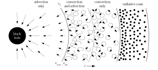
With rose, I model the accretion flow on to the BH in a quasi-star as a massive CDAF that surrounds an ADAF and central BH. In contrast to the Bondi-type quasi-stars described in Chapter 3, I refer to these models as CDAF-ADAF quasi-stars. Below, I use the results of AIQN02 and LLG04 to construct a new set of boundary conditions. The basic structure of the models is shown in Fig. 4.1. The inner radius is placed where the inward advective velocity is equal to the convective velocity. Inside this radius, all material necessarily flows inward and there is no outward transport of energy. Beyond , the structure is calculated by rose. The amount of energy is advected inwards is substantial at small radii but declines as increases. The advected energy is correctly computed but the pressure does not incorporate the gradual increase of the bulk velocity as material approaches the inner radius. As in the Bondi-type quasi-stars, the surface is necessarily radiative because of the surface boundary conditions.
4.1.1 Black hole mass and accretion rate
As in Chapter 3, the mass boundary condition is taken to be the mass of the BH and any gas inside the inner radius . According to AIQN02 and LLG04, the inner radius should be of the order of a few tens of Schwarzschild radii so the cavity mass should be negligible. Regardless, the mass boundary condition (see Section 3.1.2)
| (4.1) |
where is the density at , is implemented in the code.
The boundary between the CDAF and ADAF is characterised by the point at which the inward velocity of the flow is equal to the convective velocity (see Fig. 1 of AIQN02), where is the BH accretion rate, is the radial co-ordinate and is the density at . At this point, the total velocity of any parcel of gas must be directed inwards because the advective velocity is greater. In other words, the inward transport of energy by advection overwhelms the outward transport by convection.
The accretion rate is, by definition,
| (4.2) |
Replacing the velocity we obtain the accretion rate
| (4.3) |
which is determined entirely in terms of variables calculated by the stars code.
4.1.2 Luminosity conditions
The remaining boundary conditions are determined by the energetics of the accretion flow at the CDAF-ADAF boundary. The total luminosity throughout the flow has three components: the advective luminosity , the viscous luminosity and the convective luminosity .
Consider first the convective outer flow. The viscous flux depends on the total angular momentum flux , which is a sum of contributions from convection and advection. A defining characteristic of the CDAF is the balance between these angular momentum fluxes so the net flux is presumed to be exactly zero (AIQN02). Hence, there is no viscous flux in the CDAF. The convective luminosity is the luminosity variable determined by the code and the advective luminosity is in effect calculated by the thermal energy generation rate
| (4.4) |
where is the local luminosity in the envelope, the temperature and the specific entropy of the gas (Markovic 1995).
In the advective inner flow, convection no longer functions so is set to zero. The gas possesses angular momentum that must be removed by viscous processes. As in Section 3.1.3, the finite viscous luminosity is taken as
| (4.5) |
where is the speed of light and the radiative efficiency. As in Section 3.1.3, the fraction of mass that is converted into energy is lost from the quasi-star and its total mass decreases over time. Across the CDAF-ADAF boundary, the advective luminosity is presumed to be continuous and therefore equal on both sides. For the total luminosities to be equal, the convective luminosity in the envelope must be the same as the viscous luminosity in the ADAF . The corresponding boundary condition is
| (4.6) |
where I have used the code variable that represents the convective luminosity .
The boundary conditions are completed by balancing the luminosities inside the ADAF. As stated, there is no convective luminosity. The total flux is the sum of the advective and viscous luminosities and . The total flux is the fraction of viscous flux that is not advected on to the BH. In their integrations AIQN02 and LLG04 take the advective luminosity to be , where the Bernoulli function is in essence the total specific energy of the gas and is determined by
| (4.7) |
evaluated at the innermost meshpoint. Here, is the specific internal energy of the gas and the post-Newtonian potential (Paczyńsky & Wiita 1980) has been used to approximate the effects of general relativity. I presume that some fraction , which I call the advective efficiency, of the viscous flux is lost to advection and use the boundary condition
| (4.8) |
The fiducial value of is estimated from the work of LLG04 (Fig. 2) and this parameter is varied in Section 4.4.3.
To summarize, the three boundary conditions that replace the usual stellar conditions are
| (4.9) | |||
| (4.10) |
and
| (4.11) |
The third boundary condition is approximate because of both the form of the gravitational potential and the use of the Bernoulli function in the advective luminosity of the ADAF.
4.2 Additional physics
Based on the calculations of AIQN02 and LLG04, the inner radius of CDAF-ADAF quasi-star models is expected to be of the order of tens of Schwarzschild radii. In Chapter 3, rotation was ignored on the grounds that even Keplerian rotation at a few hundred Schwarzschild radii is dynamically insignificant at the Bondi radius when convection enforces constant specific angular momentum. The compact surroundings of the BH are now incorporated into the region modelled by the code so rotation can no longer be ignored. Its effects are included by building on the variant of the stars code developed by Potter, Tout & Eldridge (2012), rose. In Section 4.2.1, I summarize the modifications to the structure equations and derive the boundary condition for the rotation variable.
In addition, general relativity introduces effects on the order of and these must also be incorporated. This is achieved by including corrections to the structure variables, described by Thorne (1977). In Section 4.2.2, I restate the original correction factors and describe their implementation in rose. The corrections of Thorne (1977) also cater for special relativity and it should be noted that the CDAF-ADAF models do not properly treat relativistic rotation. Based on the largest rotational velocities encountered in the models, the effects of relativistic rotation are less than a few per cent. A fully relativistic description of rotation is not warranted in the presence of other approximations and the exploratory nature of this work.
4.2.1 Rotation
Potter et al. (2012) based the rotating stellar evolution code rose on the Cambridge stars code as described in Chapter 2. The effects of rotation are introduced by modifying the structure variables and equations according to prescriptions of Endal & Sofia (1978) and Meynet & Maeder (1997). Let be the area of a surface of constant pressure , the volume it contains and the radius of a sphere with the same volume. In the following, some quantities are averaged over the surface and we define
| (4.12) |
where is a surface area element. The main assumption of the structure model is the Roche approximation: the gravitational potential at radius is the same as if all the mass inside the surface were spherically distributed within .
The mass conservation equation becomes
| (4.13) |
where is the density on the constant-pressure surface and the mass it encloses. The equation of hydrostatic equilibrium changes to
| (4.14) |
where
| (4.15) |
Here, is the magnitude of the effective gravity, which is a sum of the gravitational and centrifugal accelerations.
The rotational profile of convective zones is controlled by a parameter in rose. Mixing-length theory implies that a buoyant parcel of gas retains its specific angular momentum until it disperses. This drives the rotational profile to a state of constant specific angular momentum. Magnetic fields may modify the angular momentum distribution but, because they are disregarded here, the convective zones are presumed to tend towards a state of constant specific angular momentum. Note that convection is thought strong enough that modifications owing to rotation can be ignored. The criterion for convective instability is implemented unmodified from the stars code.
Several diffusion coefficients for angular momentum mixing are implemented in rose. For CDAF-ADAF quasi-stars, we chose , where is the mixing length determined by rose in convective zones. In radiative zones, the shear component of the diffusion coefficient is determined by the model of Talon et al. (1997) and the horizontal component by the model of Maeder (2003). The parameter used in this chapter corresponds to case 4 of Potter et al. (2012).
The boundary condition for the specific angular momentum , which is now a variable in the code, is determined by conservation of angular momentum and the stipulation that convective zones are driven to constant specific angular momentum. Angular momentum redistribution is implemented as a diffusion process, which can be used to replace the rate of change of the specific angular momentum. Almost all of the envelope is fully convective throughout the evolution so the rate of change of total angular momentum of the envelope can be written as
| (4.16) | ||||
| (4.17) | ||||
| (4.18) | ||||
| (4.19) |
Above, is the rate of change of the mass of the envelope at the surface, either by accretion or mass-loss, and is the angular momentum diffusion coefficient in the convective zones, as calculated in rose. The subscript indicates variables evaluated at the innermost meshpoint, is the angular velocity at the surface and is the outer radius of the envelope. To conserve angular momentum in the envelope, the final term must be equal to zero. In normal stars, the photosphere is presumed radiative and the surface boundary condition is . At the innermost meshpoint, I apply the modified boundary condition for the rotation variable,
| (4.20) |
4.2.2 Special and general relativity
In his formulation of the equations of relativistic stellar structure, Thorne (1977) introduced two new variables and two associated differential equations to compute them. The mass variable represents the total rest mass inside radius . The total mass variable is given by the total mass inside a radius , including the contributions of the material’s nuclear binding energy, internal energy and gravitational potential. The gravitational potential is related to the metric tensor.
In terms of these variables and the standard structure variables (see Chapter 2), Thorne (1977) defined five correction factors for the structure equations. They are
| (4.21) | |||
| (4.22) | |||
| (4.23) | |||
| (4.24) |
and
| (4.25) |
The gravitational acceleration is replaced with , the pressure scale height with and the radiative gradient with . The additional structure equations are
| (4.26) |
and
| (4.27) |
The mass conservation equation becomes
| (4.28) |
and hydrostatic equilibrium is written
| (4.29) |
Here, the correction factors are simplified by taking and
| (4.30) |
which removes the need for the additional differential equations. The correction factors are implemented as
| (4.31) | |||
| (4.32) | |||
| (4.33) |
and
| (4.34) |
They are applied to the structure variables as described above. The relativistic corrections are thus not exact but still represent an improvement over the Newtonian treatment (see Section 4.3.3).
4.3 Fiducial model
In this section, I present the evolution of a quasi-star with total mass , initial BH mass and a uniform composition of hydrogen and helium by mass. The initial BH mass is larger than that of the models described in Chapter 3 because none evolved smoothly from states with interior radiative zones into a state of total convection. The advective and radiative efficiencies and are and respectively. The envelope initially has a constant specific angular momentum profile. The specific angular momentum at the inner envelope boundary is chosen so that a BH with the same specific angular momentum would have a dimensionless spin parameter (see Section 4.4.1).
The strong advective luminosity in the quasi-star envelope constitutes a departure from thermal equilibrium. Because the evolving models are not thermally relaxed, it is impossible to initialize a model in thermal equilibrium. Instead, models are initialized with a constant energy generation term of , which adds a total luminosity of about two thirds of the Eddington luminosity for a given object. The extra energy declines exponentially like so that after less than .
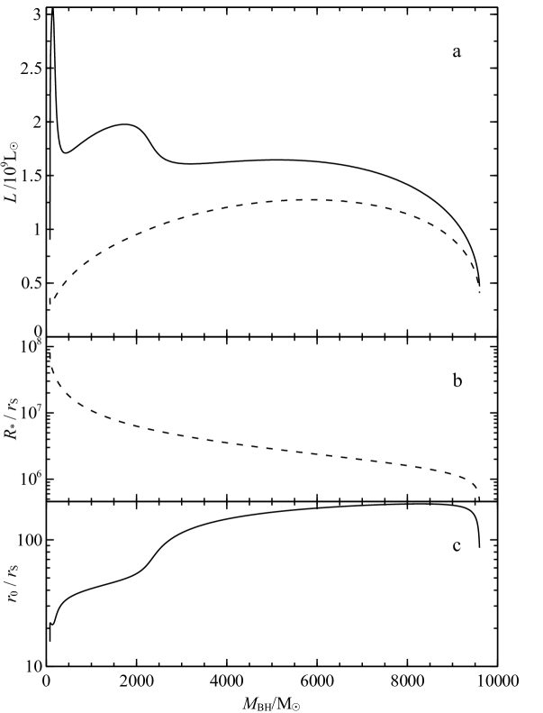
4.3.1 Evolution
Fig. 4.2 shows the evolution of the BH and surface luminosities as a function of BH mass and contains all the qualitative behaviour present in any of the model sequences. The BH luminosity exhibits three humps of decreasing maximum magnitude and increasing width. The peaks correspond to luminosities , and when , and . The BH luminosity is defined by equation (4.6) and is related to the accretion rate by so the accretion rate has peaks of , and . I refer to these local maxima, in both the BH luminosity and accretion rate, as the luminosity humps.
The evolution terminates after at which time remains in the envelope and the BH has grown to . Thus, the BH accretes all but 0.12 per cent of the available mass and this fraction varies very little between the models presented in this chapter. The nearly complete accretion of the envelope on to the BH is the most important feature of the models in this chapter. Neither is there an opacity crisis nor is the BH limited to the fractional mass limit found in Chapter 3.
It remains unclear why the accretion rate exhibits the three-humped behaviour. Just as the surface luminosity in Fig. 4.2, none of the surface properties shows any humps so they must be caused either at the inner boundary or deep inside the envelope. It is, however, difficult to disentangle the possibilities. The humps are certainly not caused by changes in the location of convective zones. Throughout the evolution, the only convectively stable region is adjacent to the surface and extends over less than by mass. I suspect that the humps are related to changes in the opacity or ionization state of the gas but I have not been able to demonstrate this. They are possibly also affected by further departures from thermal equilibrium because the thermal timescale increases both with time and towards the inner boundary. During the final hump, the thermal timescale at is a few .
Figs 4.2b and 4.2c show the locations of the inner and surface radii in units of as the BH mass grows. The inner radius has a typical magnitude of a few tens of times the Schwarzschild radius. This is consistent with the estimates and integrations by AIQN02 and LLG04. Some differences can be attributed to their results being calculated for thick discs with finite opening angles whereas the quasi-star envelopes are spherical. Variations in the rate of change of the inner radius co-incide with similar shifts in the BH luminosity and accretion rate but it is unclear whether changes in the luminosity or accretion rate affect the location of the inner radius or vice versa.
| / | / | / | / | / | / | |||
|---|---|---|---|---|---|---|---|---|
| 0.00 | 84 | 1.53 | 0.90 | 168 | 0 | .00769 | ||
| 0.29 | 1000 | 3.17 | 1.87 | 39 | .9 | 0 | .175 | |
| 0.59 | 2000 | 3.30 | 1.95 | 24 | .4 | 0 | .463 | |
| 1.65 | 5000 | 2.79 | 1.65 | 8 | .26 | 3 | .49 | |
| 3.64 | 9592 | 0.86 | 0.51 | 6 | .96 | 3 | .96 | |
| / | / | / | / | |||||
| 0.00 | 84 | 3.51 | 4 | .76 | 2 | .76 | ||
| 0.29 | 1000 | 7.27 | 4 | .43 | 4 | .59 | ||
| 0.59 | 2000 | 9.54 | 4 | .39 | 5 | .35 | ||
| 1.65 | 5000 | 12.6 | 4 | .41 | 6 | .09 | ||
| 3.64 | 9592 | 4.36 | 5 | .79 | 2 | .08 | ||
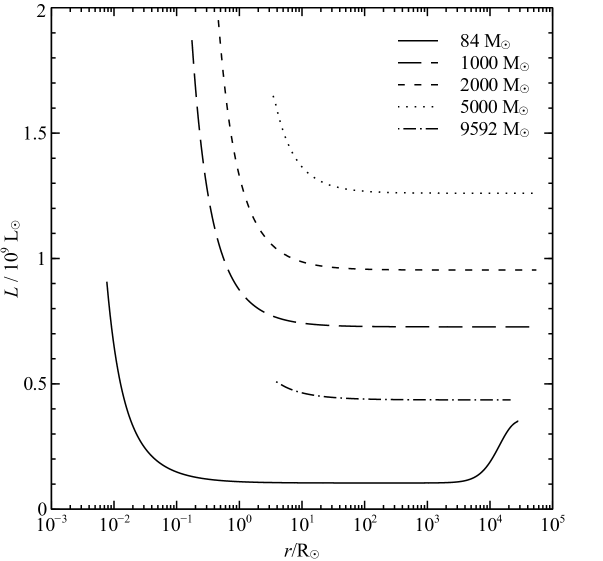
4.3.2 Structure
The variation of luminosity with radius for the models listed in Table 4.1 is shown in Fig. 4.3. The portion of the envelope that experiences strong advection is visible in each profile. In addition, the decreasing relative strength of the advection for increasing BH mass can be seen. This phenomenon is also apparent in Fig. 4.2 where the difference between the BH and surface luminosities broadly decreases as the BH grows. Note that the first luminosity profile shows a large trough because the initial constant energy generation is still present. Owing to the low density throughout the envelope, the region of the quasi-star with a significant advective luminosity is small in mass. In all the models in the fiducial run, the thermal energy generation is less than beyond and less than outside of the first of the envelope.
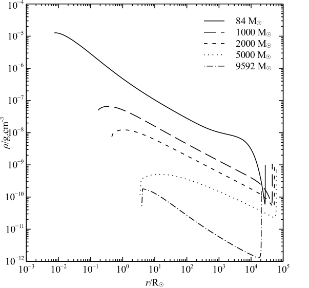
The density profiles of the models in Fig. 4.4 exhibit an inversion near the inner boundary. That is, the density increases outwards. This is theoretically unstable to the Rayleigh–Taylor instability. Density inversions are understood to appear near the surfaces of one-dimensional models of red supergiants. However, the implications of an inversion near the centre of the CDAF-ADAF quasi-stars are unclear. The models are not in a steady state, so a a sufficient increase in the advection velocity may be represented by a corresponding decrease in the density in order to keep the mass accretion rate constant throughout the model.

4.3.3 Non-rotating and non-relativistic models
To evaluate the importance of rotation and relativity in the models, three additional runs were conducted with no rotation, no corrections due to relativity or both. The evolution for each case is plotted in Fig. 4.5. Rotation only makes a significant difference during the first luminosity hump with relativity included. It otherwise plays a small role in the structure of the envelope. This is not surprising. The inner radius increases almost monotonically with , which is itself proportional to the BH mass. The specific angular momentum is roughly constant so the angular velocity falls at least as and faster if the inner radius increases as a multiple of the Schwarzschild radius. The Keplerian velocity falls off more slowly, as . Thus the ratio decreases over time, as do the structural effects of rotation.
The relativistic corrections introduce the contribution of the energy density to the gravitational potential, which is therefore steeper than its Newtonian counterpart. The inner radius is smaller, the advected luminosity greater and the accretion rate larger. At later times, when the inner radius exceeds , relativity has little effect on the structure and the accretion rates converge.
All the runs achieve roughly the same final BH mass of about . Both the non-relativistic rotating and the non-relativistic non-rotating models have lifetimes of . The non-rotating relativistic model achieves its final BH mass after , which is very similar to the lifetime of the fiducial model. The difference in the lifetimes exists mainly because of the higher accretion rates in the relativistic models.
4.4 Parameter exploration
Having established the basic properties of CDAF-ADAF quasi-stars, I now present models with different choices of the free parameters, as in Section 3.3. I begin by varying the speed of rotation in Section 4.4.1 and discussing the evolution of the BH spin. In Sections 4.4.2 and 4.4.3, I vary the radiative and advective efficiencies and, in Section 4.4.4, I consider changes to the total mass of the quasi-star, both in the initial model and during the evolution.
4.4.1 Rotation
Reasonable values for the rotation of the envelope are chosen such that a BH with the same specific angular momentum has a realistic spin. If the BH has spin parameter , its specific angular momentum is given by
| (4.35) | ||||
| (4.36) |
where is the total angular momentum of the BH. Thus, the fiducial choice corresponds to a spin parameter for an BH. Fig. 4.6 shows the evolution of central luminosity against BH mass for corresponding to initial spin parameters , and . Choices of larger than can be regarded as cases where the BH was born with a smaller specific angular momentum than the envelope. For a given angular velocity, a rigidly-rotating sphere with constant density would have times and a rigidly-rotating polytrope about times the angular momentum of a sphere with constant specific angular momentum. More centrally-condensed objects would have even smaller values so if the BH was born from a gas with such a profile it would have a smaller spin parameter to that inferred from the envelope under the presumption of constant specific angular momentum.

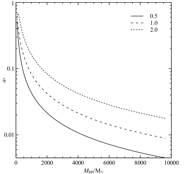
Because the angular velocity in the envelope declines rapidly, as noted in Section 4.3.3, different rotation speeds only matter near the beginning of the evolution. After the first luminosity hump, the inner radius increases significantly and, for , the evolutionary sequences are nearly indistinguishable. All the runs end with BH masses of about .
Fig. 4.7 shows the evolution of the spin parameters for the quasi-stars in Fig. 4.6. The spin of the BH is calculated by recording the total angular momentum lost at the inner boundary and presuming that it becomes part of the BH. In all three cases, the spin parameters are proportional to and this is easily explained. If a BH is born from and accretes matter with some constant specific angular momentum , its angular momentum increases as . Convective transport of angular momentum maintains a constant specific angular momentum profile. The BH’s total angular momentum is the sum of its initial angular momentum and whatever it accretes and is therefore
| (4.37) |
where a subscript represents an initial value. The BH’s spin parameter is
| (4.38) | ||||
| (4.39) |
Because the initial values are constant, it follows that the spin parameter is inversely proportional to the BH mass.
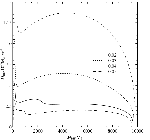
4.4.2 Radiative efficiency
The evolution of quasi-stars with radiative efficiencies , and is plotted in Fig. 4.8 along with the fiducial evolution in which . The accretion rate increases for smaller because a larger accretion rate is required to achieve the same surface luminosity. The dependence is non-linear and also related to the properties of the advective luminosity. Decreasing the radiative efficiency by one quarter to roughly doubles the accretion rate over the evolution. The surface luminosities are nearly the same so the advection luminosity must be much greater.
The non-linear effect of the radiative efficiency is understood as follows. A smaller radiative efficiency requires a larger accretion rate and the envelope contracts and becomes denser and therefore hotter. The advected luminosity is also greater and therefore even more accretion is required. If the advective luminosity were a fixed fraction of the total in the envelope, the relationship would be linear. However, the advective luminosity increases for smaller so a larger accretion rate is required than would be just to achieve the same surface luminosity.
This also explains the non-existence of any converged models for radiative efficiencies below some minimum. For the fiducial run, I could not evolve quasi-stars with radiative efficiencies below . In short, such models advect all of the luminosity inwards. Without any energy to support the envelope, it collapses on to the BH. The advection luminosity is more modest after the first BH luminosity hump so models with smaller radiative efficiencies can be constructed if the initial BH mass is larger. For this reason, the evolution with begins with initial BH mass but its subsequent evolution follows the same trends as the models with the same initial BH mass as the fiducial run.
The qualitative evolution of the runs is similar but the major quantitative difference between them is that the luminosity humps are narrower in for larger values of . For and , the first hump is wider than the total mass so there is one fewer hump in those sequences. This is probably because the envelopes are hotter and denser for smaller values of and the microphysical change that causes the three-humped behaviour is delayed.
The radiative efficiency is defined by the inner luminosity boundary condition (equation 4.6). We can also define an overall radiative efficiency . It has already been shown that varies during the evolution of a CDAF-ADAF quasi-star and the overall efficiency therefore varies too. Notably, when advection is strongest, the surface efficiency is smallest. In the runs here, the overall efficiency reaches a low of during the first luminosity hump. During the second hump, the ratio is between about and . Thereafter, where applicable, the ratio is between and . The non-existence of models with for initial BH masses less than about can be thought of as the overall efficiency being negative.

4.4.3 Advective efficiency
The advective efficiency represents the fraction of the luminosity generated in the advected zone that falls on to the BH without being radiating away. Larger values of correspond to less energy being released and should require a higher accretion rate to provide the same overall luminosity. Fig. 4.9 confirms this. The fiducial run is shown with runs where , which has a lower accretion rate, and , which has a higher rate. The accretion rates converge at larger BH masses once the role of the advective luminosity has declined. The luminosity humps occur at roughly the same points in each run but with different amplitudes.
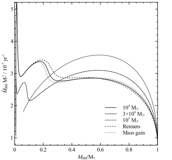
4.4.4 Initial mass and total mass loss or gain
The final free parameter that is varied is the total mass of the
quasi-star. Evolutionary sequences for quasi-stars with total initial
masses , and are plotted in
Fig. 4.10. The BH masses and accretion rater are divided by the
total masses so that the different runs can be compared. In general,
I found it difficult to find suitable parameters for successful models
with larger total masses. The quasi-star is initialized
with a BH mass of . This is nearly an
order of magnitude larger than the initial fractional BH mass in the
fiducial run. I was unable to construct models with larger total
masses and could not determine why.
More massive quasi-stars have smaller scaled accretion rates before and larger scaled accretion rates during the final luminosity hump. The humps are narrower in fractional mass but the first two are of roughly the same width (about ) in absolute BH mass. The complicated dependence of the accretion rate on total mass means there is not a simple scaling relation for quasi-stars’ lifetimes as there was for the Bondi-type quasi-stars. Measuring the lifetime from the initial fractional mass of the model, the fiducial model evolved for , the model for and the model for . The trend towards larger scaled accretion rates during the final luminosity hump appears to continue to higher masses so I expect that larger quasi-stars have shorter lifetimes than the most massive model presented here.
Fig. 4.10 also shows evolution where the quasi-star loses mass at a Reimers (1975) rate,
| (4.40) |
or gains mass at a constant rate of . The trends identified above hold for the total masses. At the end of the run, the model with mass loss contains a BH of mass inside an envelope of . The model that gains mass finishes with a BH of mass and an envelope of . As in the models that do not have additional mass loss or gain from the surface, the BH is able to consume almost all of the envelope.
4.5 Discussion
What, if anything, do CDAF-ADAF quasi-stars have in common with the Bondi-type models of Chapter 3? Regarding the structure, very little. The accretion rates of the CDAF-ADAF models are about an order of magnitude larger and the BHs ultimately accrete almost all of the available gas in the envelope. The mass limit found in Chapter 3 is robust but CDAF-ADAF quasi-stars are not in thermal equilibrium and therefore the polytropic analysis does not apply to them. While the CDAF-ADAF quasi-stars in this chapter are not necessarily more reliable, they demonstrate that the choice of the inner boundary is critical in determining the qualitative and quantitative behaviour of the envelope’s structure.
The surface behaviour of the CDAF-ADAF quasi-stars, however, is not so different from the Bondi-type models. In both cases, the surface temperatures are effectively set by the Hayashi limit and are therefore quite accurately around . More roughly, the surface luminosity is on the order of the Eddington luminosity of the quasi-star. The surface boundary condition requires that the envelope’s surface radius is on the order of . Although the details of the structure depends critically on selecting appropriate boundary conditions, the surface properties of the objects are reasonably similar. The most important quantitative difference in the evolution of the observable properties is the total lifetime, which determines the duty cycle of the quasi-star phase.
For comparison, the location of the Bondi radius can be found in the CDAF-ADAF models. In the fiducial run, the Bondi radii (where ) when and are and , respectively. For the corresponding BH masses in the fiducial Bondi-type quasi-star, the inner radii are and , which compare reasonably well. However, for , a Bondi radius cannot be found in the CDAF-ADAF models. This is consistent with the existence of a BH mass limit when the inner radius is defined through the Bondi radius but also suggests that Bondi-type models fail to capture the true behaviour of the models at higher BH masses.
The three-phase behaviour of the CDAF-ADAF models was also not seen in the Bondi-type quasi-stars and probably occurs because of changes in the advective luminosity owing to some microphysical property of the envelope material. Some models require that the first hump is avoided entirely. The high initial accretion rate might indicate that the BH generally grows at first through a very rapid accretion phase before the envelope settles into a state described by approximate hydrostatic equilibrium.
The changing advective luminosity implies that the overall radiative efficiency of accretion, defined by , is not constant. It may be possible to construct CDAF-ADAF quasi-stars by regarding , rather than , as a constant. LLG04 adopted this approach and found . In the late phases of the quasi-star evolution, such a low value of would almost certainly admit a much larger accretion rate and therefore shorter lifetimes.
4.6 Conclusion
I have presented quasi-star models that employ boundary conditions based on the global accretion solutions of AIQN02 and LLG04. An advection-dominated flow is presumed to be surrounded by a convective envelope, the structure of which is computed with approximate treatments of rotation and relativity. The behaviour of the models is qualitatively and quantitatively distinct from the Bondi-type models described in Chapter 3. In my opinion, the most important conclusion to draw here is that the results computed using near-spherical hydrostatic quasi-stars are only as good as the inner boundary conditions that they use.
In CDAF-ADAF quasi-stars, the properties of the advective luminosity dictate how the central BH evolves. The models indicate a three-phase behaviour in which the importance of advection gradually decreases. The initial hump in the accretion rate can be sufficiently large to disrupt numerical convergence. For runs with small radiative efficiencies or large total initial masses, I bypassed this phase entirely. It may correspond to a rapid initial growth of the BH before an approximately hydrostatic configuration can be established.
For all the parameters explored here, the BH ultimately accretes
nearly all of the available material. The precise fraction varies
very little with the parameters of the model and is more than
in all the models tested here. The lifetimes of the objects are only
a few millions of years so CDAF-ADAF models create larger BHs more
rapidly than Bondi-type quasi-stars. Thus, CDAF-ADAF quasi-stars can
certainly leave BHs that are massive enough to reach masses of
by redshift but whether these structures are
accurate models of the quasi-star phase is not yet established.
{savequote}[80mm]
As far as the laws of mathematics refer to reality, they are not
certain; and as far as they are certain, they do not refer to
reality.
\qauthorfrom Sidelights on Relativity,
Albert Einstein, 1922
Chapter 5 The nature of the
Schönberg–Chandrasekhar limit
Schönberg & Chandrasekhar (1942) showed that, if embedded in a polytropic stellar envelope with index , there is a maximum fractional mass that an isothermal core can achieve in hydrostatic equilibrium. This upper limit is known as the Schönberg–Chandrasekhar (SC) limit. If the core is less massive, it remains isothermal while nuclear reactions continue in a surrounding shell. If the core is more massive, it contracts until it is supported by electron degeneracy pressure or helium begins to burn at the centre. The idealised result provides an estimate of the point at which an evolved isothermal core embedded in an extended envelope begins to contract and is sufficiently accurate that it has become a well-established element of the theory of the post-main sequence evolution of stars.
In Chapter 3, I showed that the black hole (BH) masses of Bondi-type quasi-stars are subject to a robust fractional limit. I have determined why this limit exists in terms of contours of fractional core mass of solutions when plotted in the space of homology invariant variables and . I further found that the SC limit can be explained in the same way.
Fractional mass limits have been computed for a number of other polytropic solutions. Beech (1988) calculated the corresponding limit for an isothermal core surrounded by an envelope with . Eggleton, Faulkner & Cannon (1998, hereinafter EFC98) found that, when in the envelope and in the core, a fractional mass limit exists if the density decreases discontinuously at the core-envelope boundary by a factor exceeding 3. They further proposed conditions on the polytropic indices of the core and envelope that lead to fractional mass limits. I refer to all these limits, including the original result of Schönberg & Chandrasekhar (1942) as SC-like limits.
In this chapter, I present my analysis, which unifies SC-like limits and indicates that they exist in a wider range of circumstances than the handful of cases discussed in the literature. In Section 5.1, I present the new interpretation of SC-like limits. In Section 5.2, I provide a description that captures all the SC-like limits of Section 5.1 and I consider broad classes of models that must also exhibit SC-like limits. I close by discussing some implications for real stellar models when they reach SC-like limits.
5.1 Fractional mass contours in the – plane
The analysis presented here employs the plane of homology invariant variables and . A thorough exposition of its features are provided in Appendix A but I briefly review here the most important. An equation of state is polytropic if it obeys the relation
| (5.1) |
where is the pressure, the density, the polytropic index and a constant of proportionality. By defining the dimensionless temperature by , the equations of mass conservation,
| (5.2) |
and hydrostatic equilibrium,
| (5.3) |
can be written in the dimensionless forms
| (5.4) |
and
| (5.5) |
where is the central density, is the radial co-ordinate, the mass inside , is the dimensionless radius111The scale factor is usually . We have used to avoid confusion with the density jump at the core-envelope boundary, which EFC98 called . and is the dimensionless mass. The radial scale factor is defined by
| (5.6) |
Equations 5.4 and 5.5 are equivalent to the Lane–Emden equation (LEE, A.9).
Homology invariant variables and are defined by
| (5.7) |
and
| (5.8) |
and obey the differential equation
| (5.9) |
Consider the problem of fitting a polytropic envelope to a core of arbitrary mass and radius. For a given , we can regard a given point in the – plane as the interior boundary of a polytropic envelope by integrating the LEE from that point to the surface. More precisely, we can take interior conditions
| (5.10) |
so that is the density at the base of the envelope,
| (5.11) |
and
| (5.12) |
and integrate the LEE up to the first zero of , where we set . This point marks the surface of a polytropic envelope, at which is the total dimensionless mass of the solution, including the initial value . The ratio is the fractional mass of a core that occupies a dimensionless radius . By associating each point in the – plane with the value of for a polytropic envelope that starts there, we define a surface . We use the contours of this surface to characterise the SC limit.
Figs 5.1, 5.2 and 5.3 show contours of for polytropic envelopes with , and respectively, along with a selection of interior solutions that lead to SC-like limits. For the contours are dominated by the critical point and for by . Away from or all the contours at first curve away from the -axis and then tend towards straight lines.

5.1.1 The Schönberg–Chandrasekhar limit
Kippenhahn & Weigert (1990, p. 203) discuss the SC limit in terms of fractional mass contours. Cannon (1992) also explicitly described the SC limit in terms of fractional mass contours, although he employed a different set of homology-invariant variables. Fig. 5.1 shows the isothermal solution along with the fractional mass contours for envelopes. The SC limit exists because the isothermal solution only intersects fractional mass contours up to a maximum when . In other words, along the isothermal solution, the function achieves a maximum of .
The SC limit is usually derived by defining the core pressure using virial arguments and maximizing it with respect to the core radius (e.g. Kippenhahn & Weigert 1990, p. 285). Such an explanation partly describes the SC limit but our interpretation makes clear that the existence of the SC limit has as much to do with the behaviour of the envelope solutions as the isothermal core. For example, changing the polytropic index of the envelope changes the mass limit.
If the density jumps by a factor at the core-envelope boundary, and must be transformed at the edge of the core to find the base of the envelope in the – plane. That is, if , then . The contraction of the isothermal core for is included in Fig. 5.1. The inner boundary of the envelope shifts to a smaller fractional mass of about so the SC limit falls too.
The argument presented here implies that SC-like limits exist whenever an envelope is matched to a core that only intersects fractional mass contours of that envelope up to some maximum. We now use this to explain the existence of other SC-like limits.

5.1.2 Quasi-stars
In Chapter 3, I showed that the fractional BH mass limit for Bondi-type quasi-stars also exists in polytropic models. Using fractional mass contours in the – plane, I now show how the limit is essentially the same as the SC limit, at least in the case of zero mass in the cavity. When the cavity mass is included, the connection between the SC limit and the fractional BH mass limit is not clear but it is qualitatively the same and a similar mechanism is at work.
The interior boundary condition for the quasi-star models can be written as
| (5.13) |
where is a scale factor, the mass interior to and the adiabatic sound speed. The boundary condition is a fraction of the Bondi radius, where . Begelman, Rossi & Armitage (2008) used ; the models in Chapter 3 used . Accretion on to the central BH supports the envelope by radiating near the Eddington limit of the entire object so the envelope is strongly convective and the pressure is dominated by radiation. The envelope is approximately polytropic with index . Now, at the interior boundary, , , and so
| (5.14) |
Transforming to and gives and . Varying traces a straight line, parallel to the -axis. Fig. 5.1 includes the straight lines and , which correspond to and , respectively, for . The line of does not intersect all the contours of fractional core mass because many of them are positively curved. Thus, a mass limit exists, as in previous cases. For larger values of , is also larger and intersects more of the contours. The mass limit is therefore larger.
We have limited ourselves to the case where . The fractional mass contours in Figs 5.1 and 5.3 show similar behaviour. Convective envelopes are approximately adiabatic and have effective polytropic indices between and , depending on the relative importance of gas and radiation pressures. All such envelopes possess fractional mass contours that are similar to the two cases here and we conclude that a fractional mass limit for the BH exists in all realistic cases. Envelopes with have more complicated fractional mass contours so we cannot immediately draw similar conclusions. For , Fig. 5.2 shows that the fractional mass limits for quasi-star cores behave as described above only for .
In trying to move inwards, I found I could not construct models with the stars code with in equation (5.13). The reason for this can be determined from the behaviour of the polytropic limit. As increases, increases and eventually passes the critical point when the contours change from increasing along as increases to decreasing along as increases. In other words, if a polytropic envelope is integrated from small and it has . If the envelope is instead integrated from , it has and decreases if increases. When , so small inner masses correspond to envelopes with negligible envelope mass. It becomes impossible to embed a small BH inside a massive envelope. The mass limit becomes a minimum inner mass limit. For the models presented in Chapter 3, the finite mass of the BH corresponds to a finite value of that displaces the envelope slightly from the -axis. The fractional mass contours are closely packed near so a small value of introduces a minimum inner mass limit for some .
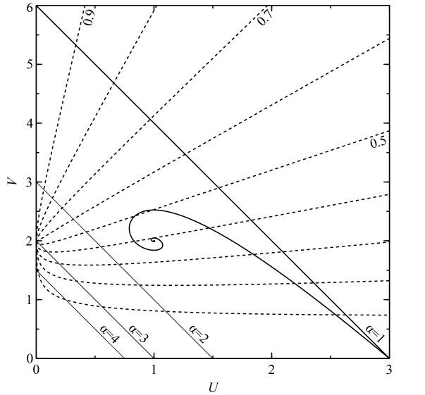
5.1.3 Other polytropic limits
Fig. 5.3 shows the fractional mass contours for , the isothermal solution and polytropes with and as used by EFC98. Beech (1988)222There appears to be an error in equation (17) of Beech (1988). The right-hand side, which should be dimensionless, has dimensions . I suspect that the appearance of in the denominator should be should actually be . The mistake does not appear to propagate into subsection equations. calculated a SC-like limit of about for an isothermal core embedded in a polytropic envelope with . Because the behaviour of fractional mass contours is similar for and , the existence of the limit is now no surprise. Inspection of Fig. 5.3 suggests , which differs from the value found by Beech (1988). This is at least partly because he included the radiation pressure of the isothermal core. The value determined here can be partly reconciled by replacing with , where is the radiation pressure with the radiation constant . The pressure appears in the definition of , which is therefore replaced with . The isothermal cores of Beech (1988) have central temperature and . The density at the core-envelope boundary is about so is about and is reduced by a similar fraction. The inclusion of radiation pressure thus explains a small fraction of the difference between the result presented here and that of Beech (1988). I am still unsure where the remainder of the difference is found.
The conclusions of EFC98 are also accommodated. The critical point separates solutions, and thus contours, with from those with . EFC98 concluded that, for envelopes, cores with are never subject to a SC limit; those with always are; and those with constitute the marginal case for which the limit exists when . The three cases are demonstrated in Fig. 5.3. When or the core solution intersects all the contours. When the core solution is everywhere below the point and only intersects contours up to . The marginal case is , for which the core solution intersects exactly and separates the values of for which the core is or is not subject to a SC-like limit. Because these conclusions are based on the critical behaviour of the solutions, which is reflected in the behaviour of the contours, the same results follow here. We have shown how they are characterised by the contours in the same way as other limits and are a particular example of our broader result. That is, we have shown that SC-like limits exist whenever the core solution fails to intersect all fractional mass contours. The cases identified by EFC98 fall within this description.
5.2 Consequences for stellar evolution
I complete this chapter by discussing four points that connect the polytropic results above to real stellar evolution. First, I identify broad classes of polytropic models that are similar to real models and subject to SC-like limits. Secondly, I discuss how stellar structure responds to a SC-like limit and, thirdly, how SC-like limits are related to the instability described by Ebert (1955), Bonnor (1956) and McCrea (1957). Finally, I introduce a theoretical test of whether a composite polytrope is at a SC-like limit.
5.2.1 General limits
The SC-like limits discussed above all exist because each locus of core-envelope boundaries only intersects fractional mass contours with smaller than some . This condition is generally satisfied whenever the curve defining the inner edge of the envelope touches but does not cross some fractional mass contour. That is, the condition is satisfied when the core solution is tangential to the contour with . This condition allows one to identify immediately the existence of additional SC-like limits and estimate their value. For example, Fig. 5.4 shows fractional mass contours for polytropic envelopes with as well as the isothermal core and the Bondi radius of a quasi-star with . By inspection, a SC-like limit exists for an isothermal core embedded in an envelope and the corresponding limit is roughly . Yabushita (1975) used such composite polytropes to model neutron stars and computed their maximum total and core masses. Although he did not explicitly calculate the maximum fractional core mass, a rough value of can be determined by fitting the core and total mass curves in his Fig. 1. The precise value of the maximum fractional core mass is . Similarly, a SC-like limit must exist for quasi-stars with envelopes. By inspection, the limit is about for , which compares well with the value determined by integrating polytropic envelopes.
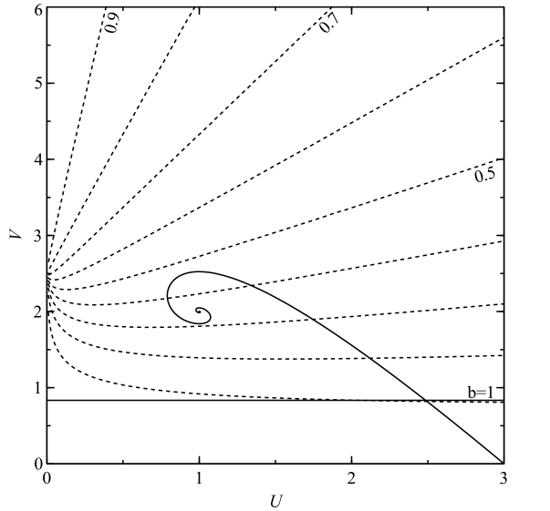
The condition for the existence of SC-like limits also identifies large classes of core solutions to which the limits apply. For example, a SC-like limit must exist whenever the core solution has everywhere , where is the polytropic index of the envelope, because there are always contours that have everywhere . Any composite polytrope with in the core and in the envelope satisfies this condition and is subject to a SC-like limit. Cores described by polytropes with envelopes, as discussed by EFC98, fail to intersect all contours. An example is plotted in Fig. 5.3, where the core solution with and clearly does not intersect contours with for envelopes with . SC-like limits exist when there is a layer with at the base of the envelope, on top of a polytropic core with . In fact, the analysis is not restricted to polytropic models so even contrived core solutions, such as , exhibit SC-like limits.
The envelope solution can also vary as long as its fractional mass contours allow the above condition to be satisfied. Although the contours are qualitatively similar for , it is not obvious that there are useful non-polytropic envelopes that have contours conducive to the existence of SC-like limits. One useful case, at least, is the convective model described by Henrich (1941). This is adiabatic with varying contributions from radiation and gas pressures. Envelopes calculated with his model behave like polytropic envelopes with near the inner boundary and near the surface.
In real stars, nuclear burning shells can meet the criteria for the existence of a SC-like limit. Nuclear reactions usually depend strongly on temperature and flatten the temperature gradient. Regions of a star where nuclear reactions are taking place therefore tend to have larger values of so SC-like limits can be present. The criteria become even stronger if the density gradient at the core-envelope boundary becomes steeper or the mean molecular weight jump becomes more pronounced. These effects shift the limiting region to smaller and where the fractional mass contours correspond to smaller fractional masses.
5.2.2 Evolution beyond the limit
What happens when an isothermal core exceeds a SC-like limit? To remain in hydrostatic equilibrium, its effective polytropic index must change. This can happen in two ways. Under suitable conditions, the inner part of the core becomes degenerate. Degenerate matter is described by a polytropic equation of state with or in relativistic or non-relativistic cases, respectively. The inner core can tend to such an equation with an isothermal layer further from the centre. A SC-like limit still exists but the isothermal layer is displaced upwards in so a larger core mass is possible.
Alternatively, the core can develop a steeper temperature gradient by departing further from thermal equilibrium. For an ideal gas the stellar structure can be described by a varying polytropic index such that so an increase in the temperature gradient decreases the effective polytropic . As long as , a SC-like limit persists but, as in the previous case, it corresponds to a larger fractional core mass. In the original SC limit, the core is isothermal so any outward temperature gradient is enough to relax the limit. For SC-like limits in general, the core can be mass-limited even if it is not in thermal equilibrium.
The structure of the envelope offers some respite from the constraints imposed by the core. For radiative envelopes, where is not much greater than , the fractional mass contours are similar to those shown in Fig. 5.1. If the envelope becomes convective, the effective polytropic index varies between and . An SC-like limit still exists but the behaviour of the fractional mass contours is less extreme near for smaller values of (compare Figs 5.1 and 5.3). Away from , contours run along smaller values of for smaller . Equivalently, is larger at a given point for smaller values of . For example, for , , whereas for , and for , . Thus, a smaller polytropic index in the envelope permits a larger fractional core mass.
5.2.3 Stability of polytropic cores
It is known that an isothermal sphere, of mass and temperature , is unstable if its radius is smaller than the critical value
| (5.15) |
where is the mass of a proton (Ebert 1955; Bonnor 1956; McCrea 1957). The sphere is unstable in the sense that, if its radius decreases, its surface pressure decreases too. In the presence of an external pressure, the sphere is compressed further and the contraction runs away. Equivalently, if the surface pressure is increased by an external agent, the sphere is doomed to collapse. The marginally stable solution is known as a Bonnor–Ebert sphere. Bonnor (1958) extended his analysis to polytropes with index and determined that a polytropic core with is unstable whenever the expression
| (5.16) |
is negative. In terms of homology-invariant variables, this is equivalent to
| (5.17) |
where and are the and co-ordinates of . The homology-invariant form of the criterion was independently derived by Hiroshi & Liu (1979). The numerator and denominator of expression (5.17) define straight lines in the – plane. The line that corresponds to the numerator passes through the origin and . The line that corresponds to the denominator is a vertical line through . For given , the critically stable polytropic core can be determined by finding the first intersection of the core with one of the two lines because infinitesimally small cores are stable. For the isothermal case, the point of intersection defines the Bonnor–Ebert sphere and similar solutions for all can be found in the same way.
The perturbations that lead to instability require only that, during the perturbation, the core has constant mass, remains in hydrostatic equilibrium and satisfies the same polytropic relation. These conditions are satisfied by the cores of composite polytropes so it is natural to ask whether the existence of Bonnor–Ebert spheres for , demonstrated by Bonnor (1958), is related to the existence for SC-like limits for , demonstrated here. I contend that they are not for several reasons. First, the limits are invoked at different points along the core solution. In the case of an isothermal core embedded in an envelope, the fractional mass of the Bonnor–Ebert sphere would be whereas the SC limit is found at . Secondly, the statements have different characters. The work of Bonnor (1958) regards stability whereas SC-like limits regard the existence of solutions. Thirdly, the stability of the isothermal core is independent of the envelope unlike SC-like limits. Although SC-like limits and Bonnor–Ebert stability are different concepts, they occur at similar points in a sequence of composite polytropes with growing cores. All else being equal, a core that reaches the critical Bonnor–Ebert mass achieves a SC-like limit shortly thereafter. Thus, if the core becomes unstable and begins to contract, it soon finds itself unable to accommodate additional mass.
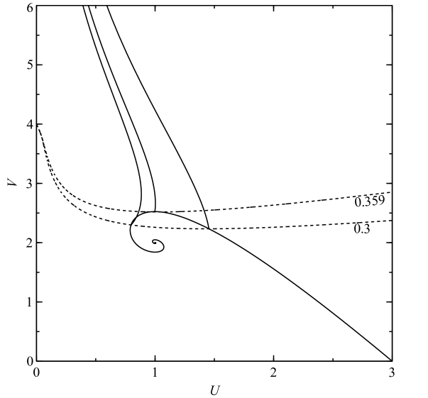
5.2.4 Identifying mass-limited models
It is possible to test whether a composite polytrope is at a SC-like limit. If the core solution touches but does not cross the contour corresponding to the given fractional core mass, the model is at a SC-like limit. That is, given the polytropic model and the index in the envelope, the fractional mass at the core-envelope boundary can be computed and the whole solution plotted with the relevant fractional contour for the envelope. The condition can be applied to determine whether the model is limited. If the condition is satisfied, extending or contracting the core can only admit a smaller fractional core mass. Fig. 5.5 demonstrates the test applied to a model at its SC limit. The core-envelope solution touches and is curved away from the contour with fractional mass so our test confirms that the model is at a limit. The other models, with , are not tangential to the contours and are therefore not at a SC-like limit.
The test can be applied to realistic stellar models and allows us to connect the purely theoretical results of this chapter with real stellar models. It is, however, difficult to identify stars that have reached a SC-like limit because the inner edge of the envelope is not clearly defined and the effective polytropic index varies throughout the envelope. In the next chapter, the test is applied to realistic stellar models from the Cambridge stars code and the results suggest that there is a connection between stars reaching SC-like limits and subsequently evolving into giants.
[80mm] I would not recommend anyone, particularly if they are in a temporary research position, to waste any time looking for a sufficient condition. \qauthorPeter Eggleton, 2000
Chapter 6 Fractional mass limits
and the structure of giants
When the core of a main-sequence star exhausts its supply of hydrogen, it undergoes a number of qualitative changes. Nuclear burning moves from the centre to a shell around the inert core and the mean molecular weight gradient at the core-envelope boundary steepens. At the same time, the envelope begins to expand increasingly quickly. With the total luminosity roughly constant, the surface temperature drops until the star reaches the Hayashi track and a deep convective zone penetrates inwards from the surface, marking the beginning of the red giant branch. The rapid decrease in surface temperature means that few stars are found in the so-called Hertzsprung gap. During this phase, a star’s envelope expands greatly, potentially by orders of magnitude, and continues to do so as it ascends the red giant branch.
Though the evolution of main-sequence stars into giants has in essence been reproduced since the pioneering calculations by Hoyle & Schwarzschild (1955), the cause of a star’s substantial expansion after leaving the main sequence remains unknown. This red giant problem continues to receive occasional attention. Some authors have claimed both to solve the problem and explain why previous solutions were incomplete only to have the same claim made against them by others. It appears that whether or not the red giant problem is an open question is itself an open question.
Some clarity is achieved by more precisely specifying the problem. In my opinion, there are in fact two red giant problems that are discussed and accusations of incomplete solutions have been directed at authors who were actually answering a different question. The first question is “why do stellar cores necessarily contract after leaving the main sequence?” The second question is “why does a modest contraction of the core lead to extensive expansion of the envelope?”
Many potential solutions have been posed (and an approximately equal number contested) to both of these problems. Eggleton & Cannon (1991) showed that if the effective polytropic index of a star is everywhere less than some , it is less centrally condensed (i.e. the ratio of central to mean density is smaller) than the polytrope of index . Eggleton (2000) further conjectured that the evolution of dwarfs into giants during shell burning therefore requires that a significant part deep in the envelope has an effective polytropic index . Because these conditions are similar to those under which SC-like limits exist, I explore in this chapter the possible connection between SC-like limits and giant formation. In Section 6.1, I summarize some ideas on the red giant problem from the last thirty years. Then, in Section 6.2, I apply the test for SC-like limits devised in Section 5.2.4 to realistic stellar models to determine if there is a deeper connection between SC-like limits and the evolution of dwarfs into giants. I close the chapter by discussing, in Section 6.3, the results with respect to the two questions above.
6.1 A brief history of the red giant problem
Eggleton & Faulkner (1981) summarized and refuted a number of potential causes for the formation of giants. They first assert that the red giant problem is not resolved by the development of convective envelopes, the development of degenerate cores, the Virial Theorem or the SC limit. The first two points are discussed below. The Virial Theorem is discounted because it regards the whole star and says nothing of the density or temperature distribution within the star. The role of the SC limit is the subject of this chapter. Eggleton & Faulkner (1981) assert that the evolution of stars into giants is caused by the formation of a molecular weight gradient and the shift from core burning to shell burning. They also concede that the evidence is complicated. First, the molecular weight gradient develops before hydrogen is exhausted in the core and only reaches a factor of two even though the envelope expands by several orders of magnitude. Secondly, despite developing a “strong” shell source, low-mass helium stars do not become giants. Finally, the burning shells in massive stars are not strong at first. Thus, to explain the red giant problem with the molecular weight gradient or shell burning, one must also explain why some stars do not become giants even when one or both of the conditions is present.
In this section, I review a handful of contributions to the literature since the summary by Eggleton & Faulkner (1981). Some are corroborations of the points they raised. Others are novel ideas. Ultimately, any discussion of the red giant problem is a contemporary snapshot of an unresolved problem. The discussion demonstrates the complicated nature of the problems of isolating cause and effect in full stellar calculations and in connecting simplified models with real physical behaviour.
6.1.1 Convection, degeneracy and thermal stability of the envelope
If the ongoing discussion shows a lack of consensus on what causes stars to become giants, at least there is some consensus on physical changes that do not lead to giant formation, neither in the sense of explaining why the core contracts nor why the expansion of the envelope is disproportionately large. First, the development of a deep convective zone adjacent to the stellar surface is not relevant. Secondly, the increasing contribution of electron degeneracy to the pressure in the core is also unrelated. Massive stars begin to expand towards giant proportions before either condition is true and low-mass stars evolve into giants even if convection is artificially suppressed in numerical models (Stancliffe et al. 2009).
Renzini (1984) suggested that the expansion of the envelope is caused by a runaway thermal instability of the envelope. He used the diagnostic to decide whether the envelope is unstable to an increased incident luminosity at the edge of the shell. His parameter is related to the thermal conductivity and therefore opacity, so he argued that the runaway expansion of the envelope is a result of radiation being locked in the envelope by increasing opacity. Only the onset of convection on the Hayashi track assuages the instability.
Already, Weiss (1989) questioned this approach by demonstrating that the approximate formula for used by Renzini (1984) is generally inaccurate, often including its sign, and there exist regions of the envelope that are supposedly unstable by this criterion but are actually stable. Renzini et al. (1992) later restated Renzini’s (1984) solution to the red giant problem with little detailed discussion of the work of Weiss (1989). Iben (1993) also pointed out that thermal instability is not a necessary condition because stars still become giants when overall thermal equilibrium is artificially enforced. For low-mass stars, there is little difference between models with and without thermal equilibrium. Thus, the thermal instability in the envelope cannot be the cause of a star’s evolution to gianthood.
The final word in the conversation of papers appears to belong to Renzini & Ritossa (1994), who argue that, while stars expand into giants when the opacity is constant or thermal instability is artificially suppressed, in these cases the core luminosity must exceed a critical value. Low-metallicity massive stars only reach sufficient luminosity after core-helium burning begins. Renzini & Ritossa (1994) claim that this supports their argument. First, this appears to be a concession that their envelope instability does not account for at least some giants. Secondly, it is not clear what the critical luminosity is or why it should exist. In fact, massive low-metallicity stellar models successfully evolve into giants at lower luminosities if nuclear transformations are stopped (which fixes the mass location of shell-burning) and only energy from expansion, contraction and hydrogen-burning is included (so that core-helium burning cannot restore thermal equilibrium). The observation of thermal instability is probably a confusion of cause and effect. Stellar envelopes expand increasingly quickly in the Hertzsprung gap and, whatever the cause, the expansion is necessarily reflected in an increasing thermal imbalance between core and envelope.
6.1.2 Molecular weight gradients, shell burning and polytropic indices
Eggleton & Faulkner (1981) already claimed that stars expand to giant dimensions because the molecular weight gradient between the core and the envelope steepens and the nuclear reactions proceed in a shell rather than the core. Eggleton & Faulkner (1981) also acknowledge that these two qualities are insufficient when isolated. A molecular weight gradient develops during the main sequence but stars only evolve into giants after hydrogen is exhausted in the core. Low-mass (less than about ) helium stars have strong burning shells but do not evolve into giants, so the burning shell alone does not cause giant behaviour. These observations are corroborated by Stancliffe et al. (2009), who show that, if the molecular weight gradient is suppressed, a Pop I stellar model does not become a giant but a model does.
Eggleton (2000) expanded on the connection of these two effects in terms of the effective polytropic index of a stellar model, where is defined by
| (6.1) |
In a perfect gas, an increase in the mean molecular weight causes an increase in . Nuclear burning has a thermostatic effect and flattens the temperature gradient where it occurs, which also increases . Eggleton (2000) demonstrated that, using the variation of with in a stellar model, one can distinguish dwarf-like models from giant-like models by the presence of substantial regions where is much greater than . The shortcoming of this argument is that it only says that a model without any such regions is dwarf-like. It is not clear how large must be or in how large a region for a star to be giant-like.
Sugimoto & Fujimoto (2000) quote similar conditions under which stellar models in the – plane cross the line where . Their claim that curves that cross this line have divergent radii is refuted by Faulkner (2005) as a mathematical misinterpretation. It is true, however, that solutions that have loops in the – plane cross this line twice. Such solutions can accommodate a greater fractional mass in the envelope and this is a characteristic of giants. However, the presence of loops has not been demonstrated to be the cause of a star’s evolution to a giant. Faulkner (2005) contests that giant structure occurs because the stellar core cannot accommodate more mass without first inflating the envelope. This is similar to the situations identified by SC-like limits.
Based on the calculation of fractional mass limits in Chapter 5, the conditions described by Eggleton (2000) correspond well with the conditions under which fractional mass limits are likely to exist. Certainly, when there is a layer between the core and envelope where , a SC-like limit exists. Whether or not a stellar model reaches the limit depends on the extent of that region. The purpose of the remainder of this chapter is to evaluate when stellar models appear to reach SC-like limits and whether it corresponds to the evolution of a star into a giant.
6.2 Fractional mass limits in realistic stellar models
Realistic stellar models are now tested for the presence of SC-like limits. In particular, I analyse – profiles of stellar models with masses between and at solar metallicity (Section 6.2.1), between and at solar metallicity (Section 6.2.2), and between and with helium instead of hydrogen (Section 6.2.3). No convective overshooting or mass loss was included and the models are initially of homogeneous composition.
The fractional mass limit test is applied by searching for the first model in the evolution for which its – profile contains a segment that is tangential to a fractional mass contour. Models shortly before and after the limit are also tested to show that the behaviour is similar to the SC limit. The fractional mass contours presume that the envelope’s effective polytropic index is . In a given model, a larger effective polytropic index would admit a smaller fractional mass earlier in a star’s evolution. The approximation of in the envelope is usually reasonable but some models have polytropic indices as low as or as high as . In these cases, the value is justified because the models ultimately exceed the limits for other choices of and the fractional mass is approximate at a similar level to errors introduced by changing the envelope’s polytropic index.
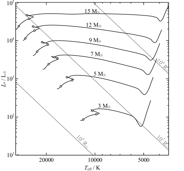
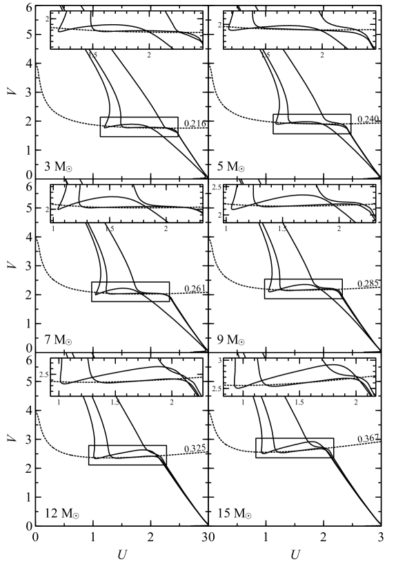
6.2.1 Intermediate-mass Population I giants
Fig. 6.1 shows evolutionary tracks for stars of solar metallicity at masses , , , , and . As each star consumes its core hydrogen, it becomes slightly brighter and redder, moving up and to the right in the Hertzsprung–Russell diagram (HRD). During the main sequence evolution, the core is convective but the convective boundary slowly retreats, leaving a composition gradient outside the convective core. When it exhausts its hydrogen, the whole core does so simultaneously and there is a phase of contraction before hydrogen shell-burning commences. The shrinking envelope briefly becomes bluer before moving redward across the Hertzsprung gap. The models were followed to the top of their ascent on the red giant branch. Note that all of these stars become red giants in the sense that they ultimately cross the Hertzsprung gap completely but the and stars ignite helium in the core before they reach the base of the red giant branch.
Fig. 6.2 shows the - profiles of the models marked with open circles in Fig. 6.1. The middle model in each case is at a SC-like limit. The molecular weight gradient extends from to so the composition profile does not define a clear core-envelope boundary. The fractional core mass is determined by finding, by eye, the first envelope contour that is tangential to a segment of the model. This process clearly identifies a particular contour and the fractional core masses are roughly consistent with those found by other measures such as the centre of the composition gradient. The models are compared to the same fractional mass contour because the core mass does not appear to change noticeably between them. In all cases, the result of the test is similar: the models approach, reach and exceed the mass derived from the polytropic contour. The masses are larger than traditional values of the core mass because the limiting region is now the base of the envelope. The limiting mass includes the shell where hydrogen shell-burning begins, which is initially quite thick.
The point in the HRD at which models reach a SC-like limit is always near core hydrogen depletion. There are two important observations to be made. First, this is earlier than the point at which most authors say a star reaches the SC limit. A star, for example, is usually thought to reach the SC limit while it crosses the Hertzsprung gap. Secondly, stars are usually thought to reach the SC limit at different points. Broadly, higher-mass stars reach the SC limit earlier in their evolution. The results presented here suggest that all intermediate-mass stars reach mass limits once hydrogen is depleted in the core. The core structure is subject to a SC-like limit during the whole evolution into a giant, irrespective of whether the core (or any other part of the star) is in thermal equilibrium.
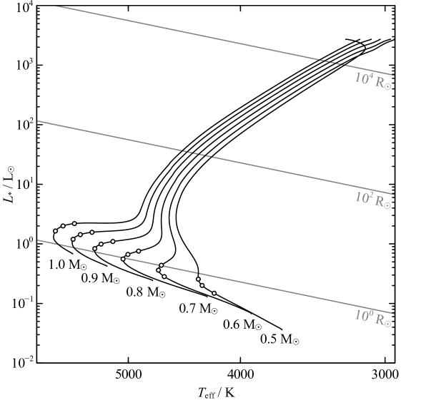
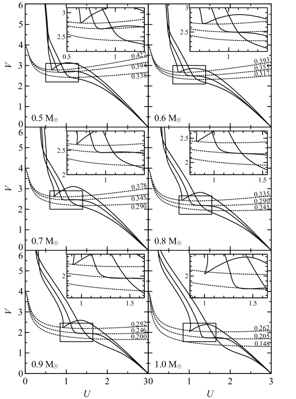
6.2.2 Low-mass Population I giants
Fig. 6.3 shows evolutionary tracks for stars of solar metallicity at masses , , , , and . The cores of these stars are convectively stable during the main sequence so there is a gradual progression from core-burning to shell-burning. Specifically, there are no blueward hooks, as in the previous section. The evolution was followed up to core helium ignition. In low-mass stars, the core becomes electron degenerate and roughly isothermal before core helium-burning begins. As a result, helium is ignited almost simultaneously across the core. The sudden, rapid and unstable increase in luminosity is known as a flash. Such flashes are a known stumbling block of the stars code.
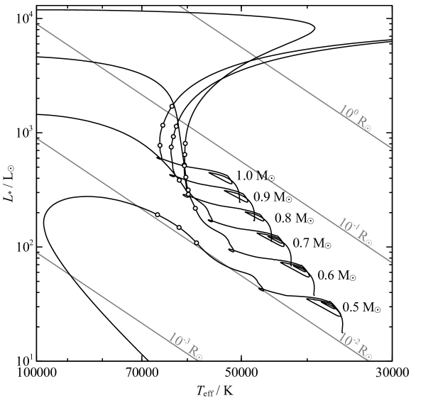

As in Section 6.2.1, Fig. 6.4 shows the - profiles of the models marked with open circles in Fig. 6.3 and the middle profile is thought to have reached a SC-like limit. The profiles bend at large because the polytropic index of the envelope changes to in the surface convection zone, which is always present. Outside the surface convection zones, the envelopes have larger polytropic indices than the intermediate-mass stars, so the fractional masses are probably a few hundredths smaller and occur when the luminosities are smaller by a few per cent. Aside from this approximation, the models all appear to reach SC-like limits shortly after hydrogen is exhausted in the core.
The track turns towards higher surface temperatures near the end of the run because the unburned hydrogen envelope contains less that 5 per cent of the total mass. The run halts because of degenerate helium ignition. Slightly less massive models do not ignite helium and evolve to the helium white dwarf cooling sequence. The fact that the model does not truly finish its life as a giant does not undermine any effort to identify why it became a giant in the first place.
6.2.3 Helium giants
Fig. 6.5 shows evolutionary tracks for helium stars with Pop I metal content and masses , , , , and . The stars have convective cores during the core helium-burning phase. As the helium nears depletion, the core convective zone extends further out, mixing in unburned helium. This extends the core burning phase. The episodes of ingestion cause loops in the theoretical HRD that are known as breathing pulses after the repeated contraction and expansion of the core. Once the core evolves past the last breathing pulse, it depletes helium completely and convection stops. Helium-shell burning begins at the small loop to the left of the breathing pulses. Models were followed either until their effective temperatures began to decrease on a white dwarf cooling track or until a surface convection zone formed, indicating that the star arrived on the helium red giant branch.
Fig. 6.6 again shows the - profiles of the models marked with open circles in Fig. 6.5. These models also appear to reach SC-like limits but only after a substantial amount of mass has been added to the core during shell burning. The connection between SC-like limits and gianthood is weaker here. Although the models appear to reach limits, they do not clearly exceed them as the hydrogen-burning models did. That is, for masses less than , the models never have - profiles where the gradient is clearly greater than a contour that passes through the nuclear burning shell. Indeed these models do not become giants although the and models do undergo some expansion. The model expands like the and models but it turns back towards the white dwarf cooling tracks when the surface temperature reaches about . As with the Pop I star, the envelope mass becomes negligible and the star is almost entirely described by the core.
The helium stars presented here indicate that stars appear to expand when they are at or near a SC-like limit. Weaker nuclear burning shells and shallow molecular weight gradients reduce the effective polytropic index and diminish the prospects of a star being subject to a SC-like limit. The response of the envelope may restore the stellar profile to a state where it is not subject to a limit, in which case it continues to become bluer until it finally moves on to a white dwarf cooling track.
6.3 Discussion
The analysis presented above suggests that stars begin to evolve into giants when they reach a SC-like limit. In this section, I discuss the combined evidence with respect to the two red giant problems. In Section 6.3.1, I address whether SC-like limits explain the contraction of the core. In Section 6.3.2, I consider how SC-like limits are related to the drastic expansion of the envelope.
6.3.1 Core contraction
Traditional discussions of the relevance of the SC limit compare the mass of the exhausted core to a fractional mass limit of . Stars of different masses reach this limit at different stages of evolution. Here, all the stellar models that begin to evolve into giants appear to reach a SC-like limit just before depleting the nuclear fuel in their cores. This implies three important distinctions from the usual interpretation of the SC limit. First, fractional mass limits like the SC limit are relevant earlier than usually thought. Secondly, the point in a star’s evolution at which the mass limit is relevant is roughly the same independent of mass. Thirdly, the limiting mass co-ordinate is located in the burning shell and does not only include the exhausted core. That all stars that evolve into giants achieve a limiting fractional mass at the same point suggests a connection between SC-like limits and evolution into giants but the issue is far from clear cut.
In the low-mass Pop I models and helium stars, SC-like limits do correlate with expansion of the envelope. Models that reach and exceed a SC-like limit start to expand even though the expansion sometimes ceases. There are many possible reasons for this. In the simplest cases, shell-burning continues to increase the core mass and the envelope becomes vanishingly small by mass. As the shell-burning declines, the limiting region (with ) vanishes and the SC-like limit is relaxed. The helium star and Pop I model demonstrate such behaviour. It can be argued that these stars started to become giants but the envelope was transformed into core material before the transition was accomplished. Another option is that the microphysics of the limiting region responds to the expansion of the envelope such that a SC-like limit is avoided and never encountered again. For example, the helium star expands slightly and briefly after core helium exhaustion but shell burning is weakened by the expansion and the envelope is processed by nuclear reactions before another limit is encountered. The star never appears to exceed a SC-like limit although it does roughly reach one. It expands only slightly during the shell-burning phase but soon turns back towards the white dwarf cooling sequence.
The intermediate-mass Pop I models also reach a limit as they exhaust their core hydrogen supplies but they briefly contract rather than expand. The envelopes do expand once shell-burning begins but not before. This suggests that SC-like limits are connected to the contraction of the core but not necessarily the expansion of the envelope. The model adhere to the same SC-like limit during the contraction so the core may be able to sustain the limit until shell-burning begins.
These conclusions are all subject to the approximations of the test. There is no well-defined core-envelope boundary at the end of the main sequence so it is not surprising that there are differences between the core masses determined by the test and masses determined by other methods. The polytropic index is certainly not constant and in some models deviates quite substantially from , which was used to test the models for fractional mass limits. A variable polytropic index might change the shape of the fractional mass contours depending on how it varies through the envelope. Despite this, the overall shape of the envelope profiles is broadly consistent with some SC-like limit even if it occurs at a slightly different point in evolution.

6.3.2 Envelope expansion
Let us now consider the other problem: why are the envelopes of red giants so extended? Fig. 6.7 shows contours of constant ratio of total radius to core radius for polytropic envelopes with . The figure is created in the same way as the figures showing contours of constant fractional mass. Here, the inverse of the fractional ratio is shown and the contours are spaced logarithmically. As an example, if the core radius is fixed, an envelope with an inner boundary along the curve is times smaller than an envelope with an inner boundary along the curve. The plot shows that the fractional surface radius increases as or decreases. The behaviour is particularly extreme near the critical point .
Given a composite polytrope for which a SC-like limit exists, there are usually two models with the same fractional core mass. Fig. 5.5 shows this for isothermal cores with fractional mass embedded in envelopes with . The two solutions have different fractional radii so, for fixed core radius, the envelope is more extended in the model for which is smaller at the core-envelope boundary. The more extended model is giant-like and the other is dwarf-like.
Realistic models are initially in the dwarf-like configuration. The feature that forces the core-envelope boundary to smaller is a large effective polytropic index between the core and the envelope. The large polytropic index means the solution tries to orbit the critical point in the – plane. Hence, if a star has a region with between the core and envelope, its radius is larger than if this region did not exist. As discussed in Section 5.2.1, shell burning and a molecular weight gradient increase the effective polytropic index and they are both connected to the large surface radii of giants. Convection drives the effective polytropic index towards , for which the critical point is closer to the point around which isothermal solutions spiral, . On the other hand, polytropic envelopes with behave less extremely near because and do not co-incide as they do for . It is not clear whether or not the envelope’s expansion is more extreme once convection develops.
The argument above offers an explanation of why the envelopes of giants are so large. It does not explain why the core-envelope boundary evolves such that the envelope becomes even larger. Do SC-like limits play a role? It has already been noted that stars expand at the same time as they reach SC-like limits. All else being equal, the core cannot accommodate more mass by continuing to larger radii because the effective polytropic index at the core-envelope boundary is too large. A change in the core’s structure is required, be it the central density, the effective polytropic index or something else, and this change might be unstable. For example, if the core contracts, its mean density increases. If the presence of a nuclear burning shell prevents the density at the core-envelope boundary from increasing by the same amount, decreases, potentially enough that the envelope’s expansion is greater than the core’s contraction. It is thus possible that, once a SC-limit has been exceeded and the core adjusts to incorporate more mass, the additional mass forces it to adjust further but I have not been able to demonstrate that this is the case.
6.4 Conclusion
Three sets of stellar models have been tested for the presence of SC-like limits. All stars that become giants appear to reach a limit shortly before the end of their core-burning phases. When the transition to shell-burning is continuous, the limit is associated with expansion of the envelope. That is, the star begins to become a giant. Whether the star continues to expand depends on whether the rest of the envelope is transformed into core material and how the burning-shell responds to the envelope’s expansion. Stars that are convective during core-burning contract until shell-burning begins, after which the envelope expands. Some stars never appear to exceed a SC-like limit and proceed directly to a white dwarf cooling sequence without any period of significant expansion.
Though the test is approximate, it suggests that SC-like limits are relevant immediately at the end of the main sequence in all stars and are determined within the burning shell or molecular weight gradient. Stars that become giants must have previously reached a SC-like limit. As with all possible explanations of the red giant problem, it is difficult to isolate cause and effect. The presence of loops, as identified by Sugimoto & Fujimoto (2000), already requires that giants reach SC-like limits at some point in their evolution but it is unclear which phenomenon, if either, is causal. Nevertheless, we have demonstrated that the original SC limit is a particular case of a broader phenomenon, that SC-like limits apply earlier in a star’s evolution than previously thought and that there is evidence for a connection between exceeding these limits and evolving into a giant. {savequote}[80mm] Now, this is not the end. It is not even the beginning of the end. But it is, perhaps, the end of the beginning. \qauthorSir Winston Churchill, 1942
Chapter 7 Conclusions
In this final chapter, I summarize the work presented in this dissertation, give it contemporary context and propose directions for future work. The initial aim of this dissertation was to examine models of quasi-stars with accurate microphysics. These models were presented in Chapters 3 and 4 and my findings are discussed in Section 7.1. In Chapter 5, I presented a detailed analysis of the fractional mass limit found in Chapter 3 and I demonstrated that it is of the same nature as the Schönberg–Chandrasekhar limit. In Chapter 6, I assessed whether realistic stellar models are subject to the limit and found evidence that the limits are connected to the evolution of starts into giants. I discuss these results in Section 7.2.
7.1 The formation of supermassive black holes
In Chapters 3 and 4, I presented models of quasi-stars constructed with the Cambridge stars code. The two sets of models made use of distinct inner boundary conditions to describe conditions at the base of the giant-like envelope. In Chapter 3, I followed the work of Begelman, Rossi & Armitage (2008) and placed the base of the envelope at the Bondi radius. In Chapter 4, I instead drew on the work of Abramowicz et al. (2002) and Lu, Li & Gu (2004) and placed the inner boundary at a theoretical transition from a convection-dominated accretion flow to an advection-dominated flow. I refer to the models of Chapters 3 and 4 as Bondi-type and CDAF-ADAF quasi-stars, respectively.
The evolution of the Bondi-type and CDAF-ADAF quasi-stars is qualitatively and quantitatively very different. Black holes (BHs) embedded in Bondi-type quasi-stars accrete about of the total mass of the quasi-star each year and respect a robust upper fractional mass limit of about , depending on the choice of parameters. In all cases, the quasi-star phase ends after a few million years. The fate of the remaining material is unclear. A further per cent or so of the quasi-star’s mass is within the Bondi radius. If the BH accretes this material, it probably does so on the order of its own Eddington-limited rate. If the material is in some way dispersed, it could return to the BH and be accreted later. Whatever the details, quasi-stars are certainly a possible mechanism by which early BHs could grow quickly enough to become the supermassive objects that power high-redshift quasars.
The BHs in CDAF-ADAF quasi-stars accrete roughly an order of magnitude faster than their Bondi-type cousins. This is because a substantial fraction of the BH luminosity is lost to the bulk flow of material towards the BH. More importantly, the BHs are not subject to any upper mass limit and ultimately accrete all of the available gas under all circumstances. They do so through a series of peaks in the accretion rate that appear to be related to the interaction of microphysical processes, such as ionization, with the inward advection of energy. The nature of these peaks depends on the choices of parameters in the boundary conditions but they do not depend closely on the rotation of the quasi-star envelope.
Despite the differences between Bondi-type and CDAF-ADAF models, both predict that quasi-stars leave BHs with masses on the order of a tenth of the total quasi-star mass and that the quasi-star phase lasts just a few million years. In addition, all models have luminosities roughly equal to the Eddington luminosity of the whole quasi-star, surface radii on the order of and effective temperatures that are consistently around . It thus appears that quasi-stars have similar outward properties regardless of their inner structure or even the details of their evolution. However, although their observable properties are not sensitive to the choice of inner boundary conditions, quasi-stars like those modelled in this dissertation are short-lived and would be difficult to find.
The most important conclusion that I draw from the work on quasi-stars summarized above is that, when regarded as spherical, hydrostatic objects, their detailed structure hinges on the conditions imposed at the inner boundary. The boundary conditions presented in Chapters 3 and 4 are reasonable but there are several ways in which modelling the inner region could be improved. First, incorporating the bulk velocity of the envelope material as a structural variable, as is the pressure or luminosity, should allow models to be followed close to the inner sonic point of the accretion flow. Markovic (1995) modelled a small black hole at the centre of the Sun with a similar technique but he solved the structure equations with a shooting method and did not integrate all the way to the Bondi radius.
Another possibility is modelling a quasi-star with three-dimensional fluid simulations. In general, solving the multi-dimensional problem is much more difficult and more computationally demanding but I believe it is a realistic possibility in the near future. Barai, Proga & Nagamine (2011) used the smoothed particle hydrodynamics code gadget-3 to model Bondi accretion on to a supermassive BH with both the sonic radius and Bondi radius resolved in the simulation. The main difference between their model and a quasi-star envelope is that the mass of gas in the accretion flow was much smaller that the mass of the BH. If this situation can be reversed, it should be possible to simulate the dynamical structure of a quasi-star for a brief moment in its evolution. Details derived from such a model could be used to corroborate or improve boundary conditions for spherically symmetric models.
The recent discovery of a bright quasar at redshift (Mortlock et al. 2011) and new simulations that suggest the first stars were less massive than previously thought Clark et al. 2011; Hosokawa et al. 2011; Stacy, Greif & Bromm 2012 both aggravate the problem of luminous quasars at high redshift. The solution must now explain how BHs grew even more rapidly from even smaller seeds. But the solution needs only a small number of such objects. The comoving space density of bright high-redshift quasars is only a few per and simulations of sufficiently large volumes indicate that, given sufficiently large BH seeds, there is enough material to feed a growing BH (Di Matteo et al. 2012).
The direct collapse of massive protogalactic clouds remains an appealing option for a solution to the problem provided that fragmentation can be prevented. Dijkstra et al. (2008) estimate that a fraction between and of sufficiently large dark matter halos are illuminated by stars and stellar mass BHs in nearby protogalaxies. Molecular hydrogen formation can be suppressed and fragmentation thus prevented. The fate of the collapsing gas then depends on the accretion rate of the central object. If it is slow enough for accreted material to relax into thermal equilibrium, a supermassive star might form and collapse directly into a massive BH. If the accretion is so rapid that only the central stellar core is relaxed, a quasi-star can form. In either case, a BH on the order of of the total mass is left.
This is not to say that other mechanisms for massive BH formation do not occur. Many protogalactic clouds can fragment into stars and, even if the initial mass function of metal-free stars is less top-heavy than previously thought, the most massive of these stars can leave BH remnants. As the hierarchical growth of large-scale structure continues, these BHs grow and migrate towards the centres of their host galaxies via dynamical friction. There might exist a currently undetected population of smaller BHs that power less luminous quasars. For the problem of the bright high-redshift objects that are already known, however, I believe the direct collapse mechanism is currently the strongest candidate solution.
7.2 The red giant problem
The quasi-star models presented in Chapter 3 exhibit a robust upper limit to the fractional mass of the inner BH. In Chapter 5, I showed how this limit is, in essence, the same as the Schönberg–Chandrasekhar limit. I further demonstrated that both limits are particular examples of the same general phenomenon. I refer to all such limits as SC-like limits. By considering the contours of constant fractional mass of polytropic envelopes, it is straightforward to determine whether a given core solution corresponds to a SC-like limit, even when the core solution itself is not polytropic. An additional product of my analysis is that, given a composite polytrope, one can test whether the model is at a SC-like limit. In Chapter 6, I applied this test, albeit approximately, to realistic stellar models and found evidence that there is a connection between a star reaching a SC-like limit and evolving into a giant. In a sense, Chapter 5 contains a strong theoretical result and Chapter 6 a weaker practical one.
The difficulty in resolving the red giant problem lies in distinguishing cause and effect. Any star that becomes a red giant must have previously reached a SC-like limit because loops are always present in the – profiles of giants. However, this sheds no light on whether a star expands into a giant because of the SC-like limit. Furthermore, the test that is applied in Chapter 6 suffers from two drawbacks. First, the effective polytropic index in the envelope of a realistic stellar model varies. Secondly, the models appear to reach the limit before a clear core-envelope boundary has developed. Despite these flaws, my analysis does indicate a connection between SC-like limits and gianthood. Stars that expand appear to do so when they reach SC-like limits. Whether a star continues to expand and evolve into a giant depends on the detailed response of envelope to its own expansion. For example, if the density in the burning shell decreases too much, nuclear reactions cease and a dwarf-like structure is restored. The SC-like limit might therefore address the question of why a star begins to become a giant but it offers no clear answers to the question of why giants become so extended while the contraction of the core remains moderate.
Some of these shortcomings could be addressed with further work. The test could be applied to realistic models for a range of indices simultaneously. I doubt, however, that this would be enlightening given that the behaviour of the envelope solutions is qualitatively similar across all the polytropic indices encountered in realistic giant envelopes. It may be more useful to investigate the behaviour of the contours when the effective polytropic index is allowed to vary continuously. These envelope solutions would be a better approximation to realistic envelopes and would more accurately identify the point at which a star reaches a SC-like limit.
Confronted with a long-standing problem that has already drawn and still occasionally draws detailed study, it is difficult to imagine a straightforward solution. I believe that progress is only achieved by a meticulous study of stars that do and do not become giants. Such a survey should include both realistic models and contrived models where specific physical effects or evolutionary processes are numerically isolated or removed. If a new hypothesis is formed, it should be thoroughly tested in the cases where it makes predictions, even if the predictions are only relevant in contrived or unphysical models. The red giant problem will not be solved easily but the work presented in this dissertation at least provides new clues to the answer.
References
- Abel et al. (2002) Abel T., Bryan G. L., Norman M. L., 2002, Sci, 295, 93
- Abramowicz et al. (2002) Abramowicz M. A., Igumenshchev I. V., Quataert E., Narayan R., 2002, ApJ, 565, 1101
- Alexander & Ferguson (1994) Alexander D. R., Ferguson J. W., 1994, ApJ, 437, 879
- Appenzeller & Fricke (1971) Appenzeller I., Fricke K., 1971, A&A, 12, 488
- Baraffe et al. (2001) Baraffe I., Heger A., Woosley S. E., 2001, ApJ, 550, 890
- Barai et al. (2011) Barai P., Proga D., Nagamine K., 2011, MNRAS, 418, 591
- Beech (1988) Beech M., 1988, Ap&SS, 147, 219
- Begelman (2010) Begelman M. C., 2010, MNRAS, 402, 673
- Begelman & Shlosman (2009) Begelman M. C., Shlosman I., 2009, ApJL, 702, L5
- Begelman et al. (2006) Begelman M. C., Volonteri M., Rees M. J., 2006, MNRAS, 370, 289
- Begelman et al. (2008) Begelman M. C., Rossi E. M., Armitage P. J., 2008, MNRAS, 387, 1649
- Böhm-Vitense (1958) Böhm-Vitense E., 1958, Zeit. Ast., 46, 108
- Bond et al. (1984) Bond J. R., Arnett W. D., Carr B. J., 1984, ApJ, 280, 825
- Bondi (1952) Bondi H., 1952, MNRAS, 112, 195
- Bonnor (1956) Bonnor W. B., 1956, MNRAS, 116, 351
- Bonnor (1958) Bonnor W. B., 1958, MNRAS, 118, 523
- Boylan-Kolchin et al. (2009) Boylan-Kolchin M., Springel V., White S. D. M., Jenkins A., Lemson G., 2009, MNRAS, 398, 1150
- Bromley et al. (2004) Bromley J. M., Somerville R. S., Fabian A. C., 2004, MNRAS, 350, 456
- Bromm & Larson (2004) Bromm V., Larson R. B., 2004, ARA&A, 42, 79
- Bromm et al. (1999) Bromm V., Coppi P. S., Larson R. B., 1999, ApJL, 527, L5
- Buchler & Yueh (1976) Buchler J. R., Yueh W. R., 1976, ApJ, 210, 440
- Cannon (1992) Cannon R. C., 1992, Ph.D. thesis, University of Cambridge
- Caughlan & Fowler (1988) Caughlan G. R., Fowler W. A., 1988, At. Data Nucl. Data Tables, 40, 283
- Chandrasekhar (1939) Chandrasekhar S., 1939, An Introduction to the Study of Stellar Structure. Chicago Univ. Press, Chicago
- Chandrasekhar (1964) Chandrasekhar S., 1964, ApJ, 140, 417
- Chatzopoulos & Wheeler (2012) Chatzopoulos E., Wheeler J. C., 2012, ApJ, 748, 42
- Clark et al. (2008) Clark P. C., Glover S. C. O., Klessen R. S., 2008, ApJ, 672, 757
- Clark et al. (2011) Clark P. C., Glover S. C. O., Smith R. J., Greif T. H., Klessen R. S., Bromm V., 2011, Sci, 331, 1040
- Coc et al. (2004) Coc A., Vangioni-Flam E., Descouvemont P., Adahchour A., Angulo C., 2004, ApJ, 600, 544
- Cox & Giuli (1968) Cox J. P., Giuli R. T., 1968, Principles of Stellar Structure. Gordon & Breach, New York
- Devecchi & Volonteri (2009) Devecchi B., Volonteri M., 2009, ApJ, 694, 302
- Di Matteo et al. (2012) Di Matteo T., Khandai N., DeGraf C., Feng Y., Croft R. A. C., Lopez J., Springel V., 2012, ApJL, 745, L29
- Dijkstra et al. (2008) Dijkstra M., Haiman Z., Mesinger A., Wyithe J. S. B., 2008, MNRAS, 391, 1961
- Ebert (1955) Ebert R., 1955, Z. Astrophys., 37, 217
- Eddington (1918) Eddington A. S., 1918, ApJ, 48, 205
- Eggleton (1971) Eggleton P. P., 1971, MNRAS, 151, 351
- Eggleton (1972) Eggleton P. P., 1972, MNRAS, 156, 361
- Eggleton (1973) Eggleton P. P., 1973, MNRAS, 163, 279
- Eggleton (2000) Eggleton P. P., 2000, in M. Livio, ed., Unsolved Problems in Stellar Evolution. Cambridge Univ. Press, Cambridge, p. 172
- Eggleton & Cannon (1991) Eggleton P. P., Cannon R. C., 1991, ApJ, 383, 757
- Eggleton & Faulkner (1981) Eggleton P. P., Faulkner J., 1981, in I. Iben Jr., A. Renzini, eds, Physical Processes in Red Giants. Reidel, Dordrecht, p. 179
- Eggleton et al. (1973) Eggleton P. P., Faulkner J., Flannery B. P., 1973, A&A, 23, 325
- Eggleton et al. (1998) Eggleton P. P., Faulkner J., Cannon R. C., 1998, MNRAS, 298, 831
- Eldridge & Tout (2004) Eldridge J. J., Tout C. A., 2004, MNRAS, 348, 201
- Endal & Sofia (1978) Endal A. S., Sofia S., 1978, ApJ, 220, 279
- Fan et al. (2006) Fan X., Strauss M. A., Richards G. T., Hennawi J. F., Becker R. H., 2006, AJ, 131, 1203
- Faulkner (2005) Faulkner J., 2005, in Gough, D., ed., The Scientific Legacy of Fred Hoyle. Cambridge Univ. Press, Cambridge, p. 149
- Flammang (1982) Flammang R. A., 1982, MNRAS, 199, 833
- Fowler (1964) Fowler W. A., 1964, Rev. Mod. Phys., 36, 545
- Freese et al. (2008) Freese K., Bodenheimer P., Spolyar D., Gondolo P., 2008, ApJL, 685, L101
- Fricke (1973) Fricke K. J., 1973, ApJ, 183, 941
- Fricke (1974) Fricke K. J., 1974, ApJ, 189, 535
- Fryer et al. (2001) Fryer C. L., Woosley S. E., Heger A., 2001, ApJ, 550, 372
- Gammie et al. (2004) Gammie C. F., Shapiro S. L., McKinney J. C., 2004, ApJ, 602, 312
- Haiman & Loeb (2001) Haiman Z., Loeb A., 2001, ApJ, 552, 459
- Han et al. (1994) Han Z., Podsiadlowski P., Eggleton P. P., 1994, MNRAS, 270, 121
- Heger & Woosley (2002) Heger A., Woosley S. E., 2002, ApJ, 567, 532
- Heger et al. (2003) Heger A., Fryer C. L., Woosley S. E., Langer N., Hartmann D. H., 2003, ApJ, 591, 288
- Henrich (1941) Henrich L. R., 1941, ApJ, 93, 483
- Henyey et al. (1959) Henyey L. G., Wilets L., Böhm K. H., Lelevier R., Levee R. D., 1959, ApJ, 129, 628
- Hiroshi & Liu (1979) Hiroshi K., Liu C. P., 1979, Chinese Astronomy, 3, 77
- Horedt (1987) Horedt G. P., 1987, A&A, 177, 117
- Horedt (2004) Horedt G. P., 2004, Polytropes: Applications in Astrophysics and Related Fields. Kluwer, Dordrecht
- Hosokawa et al. (2011) Hosokawa T., Omukai K., Yoshida N., Yorke H. W., 2011, Sci, 334, 1250
- Hosokawa et al. (2012) Hosokawa T., Omukai K., Yorke H. W., 2012, ArXiv e-prints
- Hoyle & Fowler (1963) Hoyle F., Fowler W. A., 1963, MNRAS, 125, 169
- Hoyle & Schwarzschild (1955) Hoyle F., Schwarzschild M., 1955, ApJS, 2, 1
- Huntley & Saslaw (1975) Huntley J. M., Saslaw W. C., 1975, ApJ, 199, 328
- Iben (1993) Iben Jr. I., 1993, ApJ, 415, 767
- Iglesias & Rogers (1996) Iglesias C. A., Rogers F. J., 1996, ApJ, 464, 943
- Itoh & Kohyama (1983) Itoh N., Kohyama Y., 1983, ApJ, 275, 858
- Itoh et al. (1989) Itoh N., Adachi T., Nakagawa M., Kohyama Y., Munakata H., 1989, ApJ, 339, 354
- Itoh et al. (1992) Itoh N., Mutoh H., Hikita A., Kohyama Y., 1992, ApJ, 395, 622
- Itoh et al. (1996) Itoh N., Hayashi H., Nishikawa A., Kohyama Y., 1996, ApJS, 102, 411
- Jiang et al. (2008) Jiang L. et al., 2008, AJ, 135, 1057
- Johnson & Bromm (2007) Johnson J. L., Bromm V., 2007, MNRAS, 374, 1557
- Johnson et al. (2011) Johnson J. L., Khochfar S., Greif T. H., Durier F., 2011, MNRAS, 410, 919
- Kim et al. (2009) Kim J., Park C., Gott III J. R., Dubinski J., 2009, ApJ, 701, 1547
- Kippenhahn & Weigert (1990) Kippenhahn R., Weigert A., 1990, Stellar Structure and Evolution. Springer-Verlag, Berlin
- Komatsu et al. (2011) Komatsu E. et al., 2011, ApJS, 192, 18
- Kowalski et al. (2008) Kowalski M. et al., 2008, ApJ, 686, 749
- Kudritzki (2002) Kudritzki R. P., 2002, ApJ, 577, 389
- Langer (1997) Langer N., 1997, in A. Nota, H. Lamers, eds, Luminous Blue Variables: Massive Stars in Transition. ASP Conf. Ser., Vol. 120, p. 83
- Larson et al. (2011) Larson D. et al., 2011, ApJS, 192, 16
- Loeb & Rasio (1994) Loeb A., Rasio F. A., 1994, ApJ, 432, 52
- Lu et al. (2004) Lu J. F., Li S. L., Gu W. M., 2004, MNRAS, 352, 147
- Lynden-Bell (1969) Lynden-Bell D., 1969, Nat, 223, 690
- Machacek et al. (2001) Machacek M. E., Bryan G. L., Abel T., 2001, ApJ, 548, 509
- Maeder (2003) Maeder A., 2003, A&A, 399, 263
- Marigo (2002) Marigo P., 2002, A&A, 387, 507
- Marigo et al. (2001) Marigo P., Girardi L., Chiosi C., Wood P. R., 2001, A&A, 371, 152
- Marigo et al. (2003) Marigo P., Chiosi C., Kudritzki R. P., 2003, A&A, 399, 617
- Markovic (1995) Markovic D., 1995, MNRAS, 277, 25
- Mayer et al. (2010) Mayer L., Kazantzidis S., Escala A., Callegari S., 2010, Nat, 466, 1082
- McCrea (1957) McCrea W. H., 1957, MNRAS, 117, 562
- Meynet & Maeder (1997) Meynet G., Maeder A., 1997, A&A, 321, 465
- Milosavljević et al. (2009a) Milosavljević M., Bromm V., Couch S. M., Oh S. P., 2009a, ApJ, 698, 766
- Milosavljević et al. (2009b) Milosavljević M., Couch S. M., Bromm V., 2009b, ApJL, 696, L146
- Mortlock et al. (2011) Mortlock D. J. et al., 2011, Nat, 474, 616
- Munakata et al. (1987) Munakata H., Kohyama Y., Itoh N., 1987, ApJ, 316, 708
- Narayan & McClintock (2008) Narayan R., McClintock J. E., 2008, New Astronomy Review, 51, 733
- Narayan & Yi (1994) Narayan R., Yi I., 1994, ApJL, 428, L13
- Narayan et al. (2000) Narayan R., Igumenshchev I. V., Abramowicz M. A., 2000, ApJ, 539, 798
- Ohkubo et al. (2006) Ohkubo T., Umeda H., Maeda K., Nomoto K., Suzuki T., Tsuruta S., Rees M. J., 2006, ApJ, 645, 1352
- Ostriker & Peebles (1973) Ostriker J. P., Peebles P. J. E., 1973, ApJ, 186, 467
- Owocki (2003) Owocki S. P., 2003, in K. van der Hucht, A. Herrero, C. Esteban, eds, A Massive Star Odyssey: From Main Sequence to Supernova. IAU Symp., Vol. 212, p. 281
- Paczyńsky & Wiita (1980) Paczyńsky B., Wiita P. J., 1980, A&A, 88, 23
- Peebles & Ratra (2003) Peebles P. J., Ratra B., 2003, Rev. Mod. Phys., 75, 559
- Percival et al. (2010) Percival W. J. et al., 2010, MNRAS, 401, 2148
- Pols et al. (1995) Pols O. R., Tout C. A., Eggleton P. P., Han Z., 1995, MNRAS, 274, 964
- Potter et al. (2012) Potter A. T., Tout C. A., Eldridge J. J., 2012, MNRAS, 419, 748
- Press & Schechter (1974) Press W. H., Schechter P., 1974, ApJ, 187, 425
- Quataert & Gruzinov (2000) Quataert E., Gruzinov A., 2000, ApJ, 539, 809
- Rees (1978) Rees M. J., 1978, Phys. Scr., 17, 193
- Rees & Ostriker (1977) Rees M. J., Ostriker J. P., 1977, MNRAS, 179, 541
- Regan & Haehnelt (2009a) Regan J. A., Haehnelt M. G., 2009a, MNRAS, 396, 343
- Regan & Haehnelt (2009b) Regan J. A., Haehnelt M. G., 2009b, MNRAS, 393, 858
- Reimers (1975) Reimers D., 1975, Memoires of the Societe Royale des Sciences de Liege, 8, 369
- Renzini (1984) Renzini A., 1984, in A. Maeder, A. Renzini, eds, Observational Tests of the Stellar Evolution Theory. IAU Symp., Vol. 105, p. 21
- Renzini & Ritossa (1994) Renzini A., Ritossa C., 1994, ApJ, 433, 293
- Renzini et al. (1992) Renzini A., Greggio L., Ritossa C., Ferrario L., 1992, ApJ, 400, 280
- Salpeter (1964) Salpeter E. E., 1964, ApJ, 140, 796
- Schleicher et al. (2010) Schleicher D. R. G., Spaans M., Glover S. C. O., 2010, ApJL, 712, L69
- Schönberg & Chandrasekhar (1942) Schönberg M., Chandrasekhar S., 1942, ApJ, 96, 161
- Shang et al. (2010) Shang C., Bryan G. L., Haiman Z., 2010, MNRAS, 402, 1249
- Shapiro (2004) Shapiro S. L., 2004, in L.C. Ho, ed., Coevolution of Black Holes and Galaxies. Cambridge Univ. Press, Cambridge, p. 103
- Shibata & Shapiro (2002) Shibata M., Shapiro S. L., 2002, ApJL, 572, L39
- Shlosman et al. (1989) Shlosman I., Frank J., Begelman M. C., 1989, Nat, 338, 45
- Siess et al. (2002) Siess L., Livio M., Lattanzio J., 2002, ApJ, 570, 329
- Sijacki et al. (2009) Sijacki D., Springel V., Haehnelt M. G., 2009, MNRAS, 400, 100
- Silk & Rees (1998) Silk J., Rees M. J., 1998, A&A, 331, L1
- Sonoi & Umeda (2012) Sonoi T., Umeda H., 2012, MNRAS, 421, L34
- Spaans & Silk (2006) Spaans M., Silk J., 2006, ApJ, 652, 902
- Spolyar et al. (2008) Spolyar D., Freese K., Gondolo P., 2008, Phys. Rev. Lett., 100, 051101
- Springel et al. (2005) Springel V. et al., 2005, Nat, 435, 629
- Stacy et al. (2011) Stacy A., Bromm V., Loeb A., 2011, MNRAS, 413, 543
- Stacy et al. (2012) Stacy A., Greif T. H., Bromm V., 2012, MNRAS, 2508
- Stancliffe & Eldridge (2009) Stancliffe R. J., Eldridge J. J., 2009, MNRAS, 396, 1699
- Stancliffe & Glebbeek (2008) Stancliffe R. J., Glebbeek E., 2008, MNRAS, 389, 1828
- Stancliffe et al. (2005) Stancliffe R. J., Lugaro M., Ugalde C., Tout C. A., Görres J., Wiescher M., 2005, MNRAS, 360, 375
- Stancliffe et al. (2009) Stancliffe R. J., Chieffi A., Lattanzio J. C., Church R. P., 2009, PASA, 26, 203
- Strogatz (1994) Strogatz S. H., 1994, Nonlinear Dynamics and Chaos: with Applications to Physics, Biology, Chemistry and Engineering. Perseus Books, Reading, MA
- Sugimoto & Fujimoto (2000) Sugimoto D., Fujimoto M. Y., 2000, ApJ, 538, 837
- Talon et al. (1997) Talon S., Zahn J. P., Maeder A., Meynet G., 1997, A&A, 322, 209
- Tanaka & Haiman (2009) Tanaka T., Haiman Z., 2009, ApJ, 696, 1798
- Tegmark et al. (1997) Tegmark M., Silk J., Rees M. J., Blanchard A., Abel T., Palla F., 1997, ApJ, 474, 1
- Thorne (1977) Thorne K. S., 1977, ApJ, 212, 825
- Thorne & Żytkow (1977) Thorne K. S., Żytkow A. N., 1977, ApJ, 212, 832
- Volonteri (2010) Volonteri M., 2010, A&A Rev., 18, 279
- Volonteri & Rees (2005) Volonteri M., Rees M. J., 2005, ApJ, 633, 624
- Volonteri et al. (2003) Volonteri M., Haardt F., Madau P., 2003, ApJ, 582, 559
- Wang et al. (2009) Wang J. M. et al., 2009, ApJL, 697, L141
- Weiss (1989) Weiss A., 1989, A&A, 209, 135
- White & Rees (1978) White S. D. M., Rees M. J., 1978, MNRAS, 183, 341
- Willott et al. (2010) Willott C. J. et al., 2010, AJ, 139, 906
- Wise & Abel (2007) Wise J. H., Abel T., 2007, ApJ, 665, 899
- Wise et al. (2008) Wise J. H., Turk M. J., Abel T., 2008, ApJ, 682, 745
- Yabushita (1975) Yabushita S., 1975, MNRAS, 172, 441
[60mm] … by means of that gruesome tool: the – plane! \qauthorMartin Schwarzschild, 1965
Appendix A Polytropes and the – plane
The analysis in Chapters 5 and 6 makes extensive use of solutions of the Lane–Emden equation in the plane of homology-invariant variables and . In this appendix, I provide the background material for that analysis. I derive the Lane–Emden equation (LEE) from hydrostatic equilibrium and mass conservation, introduce homology invariant variables and and explain their physical meaning, present the homology invariant transformation of the equation and study its solutions in the – plane. I hope that, by presenting concisely the details of the – plane in a context where it is usefully applied, I might partly remove its stigma as ‘that gruesome tool’.111Faulkner (2005) explains that Martin Schwarzschild described the – plane as such in a referee’s report in 1965. The same quote is presumably the citation by Eggleton et al. (1998) of ‘(Schwarzschild 1965, private communication)’.
A.1 The Lane–Emden equation
Consider a star that obeys everywhere a polytropic equation of state,
| (A.1) |
where is the pressure, the density, the polytropic index and a constant of proportionality. A polytropic equation of state approximates a fluid that is between the adiabatic and isothermal limits. Shallower temperature gradients correspond to larger effective polytropic indices and the isothermal case (zero temperature gradient) corresponds to . In this case, the equation of state must be transformed differently but the limit is well-defined when working in the with homology invariant variables in the – plane.
Real stars are locally polytropic in the sense that an effective polytropic index can be defined at each point by
| (A.2) |
When the star is globally polytropic, this definition reproduces the polytropic index. Certain conditions correspond to certain values of . In convective zones, the temperature gradient is approximately adiabatic, so an ideal gas without radiation has and pure radiation has . Real stars are more radiation-dominated towards the centre and varies between these limiting values in convection zones. In radiative zones, can also depend on the opacity or energy generation rate. It can be shown, for example, that for a polytropic model with uniform energy generation and a Kramer’s opacity law, ranges from for a pure ideal gas to for pure radiation (Horedt 2004, p. 556). Nuclear burning shells and ionisation regions have shallow temperature gradients and therefore large values of . Thus, the effective polytropic index can vary widely within a star.
Consider the equations of mass conservation,
| (A.3) |
and hydrostatic equilibrium,
| (A.4) |
where is the distance from the centre of the star and is the mass within a concentric sphere of radius . One can define the dimensionless temperature222This is by the analogy to an ideal gas, for which . by , where is the density at the centre of the star. By re-arranging and differentiating the equation of hydrostatic equilibrium, we obtain
| (A.5) |
By using mass conservation to replace and dividing both sides by we obtain
| (A.6) |
Substituting the pressure via the polytropic equation of state, replacing the density with the dimensionless temperature and defining the dimensionless radius333The scale factor is usually denoted by . Here, the variable is used to avoid confusion with the density jump at the core-envelope boundary, which Eggleton et al. (1998) called . , we write
| (A.7) |
which we render dimensionless by choosing
| (A.8) |
The dimensionless differential equation is the LEE,
| (A.9) |
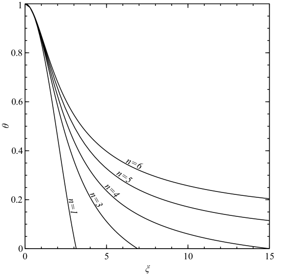
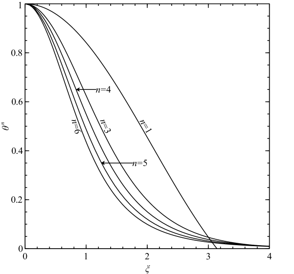
Let us define the dimensionless mass . Introducing the dimensionless mass, temperature and radius directly into equations (A.3) and (A.4) allows us to write
| (A.10) |
and
| (A.11) |
The expression of the LEE as two first-order equations (A.10 and A.11) preserves the physical meaning of the equations and easily permits arbitrary boundary conditions for the inner mass and radius.
Solutions of the LEE that are regular at the centre have
. The subset of solutions that extend from the centre
to infinite radius or the first zero of are polytropes
of index . I refer to solutions that are regular at the centre but
truncated at some finite radius as polytropic cores.
Conversely, solutions that extend from a finite radius to infinity or
the first zero of are polytropic envelopes. Models in
which polytropic cores are matched to polytropic envelopes are
referred to as composite polytropes.
For polytropes are finite in both mass and radius
while for they are infinite in mass and radius. The case
represents the threshold between the two: it has a finite mass but
infinite radius.
A.2 Homology and homology-invariant variables
If, given a solution to a differential equation, further solutions can be found by rescaling the given solution, the differential equation is said to admit an homology transformation (Chandrasekhar 1939, p. 102). Two solutions related in this way are homologous; the similarity between them is homology. The LEE admits an homology and the appropriate scaling relation is now derived.
Consider the usual second-order form of the LEE (equation A.9) with a solution . If there is a further solution of the form , it must satisfy the equation
| (A.12) |
The left-hand side can be manipulated as follows.
| (A.13) | ||||
| (A.14) | ||||
| (A.15) | ||||
| (A.16) |
If the last line is to be the same as , we must have and hence . The homology transformation of the LEE for is therefore .
To find the transformation for , we seek that satisfies
| (A.17) |
and
| (A.18) |
The left-hand sides of the two equations can be considered separately and simultaneously.
| (A.19) | ||||||
| (A.20) | ||||||
| (A.21) | ||||||
| (A.22) | ||||||
| (A.23) | ||||||
| (A.24) |
In both cases, the remaining exponent of must be zero and thus . That is, the homology transformation for is .
By choosing variables that are invariant under the homology transformation, the LEE can be formulated as a single first-order equation that captures all essential behaviour. The variables used here are
| (A.25) |
and
| (A.26) |
where is the mean density of the material inside . Although and have been defined to reduce the order of the LEE, the corresponding physical definitions make them meaningful for discussions of any stellar model. A brief excursion is made to explain these definitions.
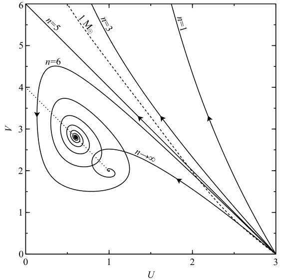
The physical variables are all positive so only the first quadrant of the – plane is of interest. The variable is three times the ratio of the local density to the mean density inside that radius. As , so also and thus . We expect the density of a stellar model to decrease with radius, so and hence . The variable is related to the ratio of specific gravitational binding energy to specific internal energy. At the centre, and are finite and , so . Thus, in all physical solutions that extend to , the centre corresponds to . If an interior solution has everywhere smaller than the appropriate polytrope, it behaves as if it has a finite point mass at its centre. Huntley & Saslaw (1975) referred to similar models, integrated outwards from a finite radius, as loaded polytropes. If a solution has everywhere greater than the polytrope, it reaches zero mass before zero radius. Such solutions have a massless core with finite radius, which is unphysical. At the surface, so too. On the other hand, takes a finite value but so . All realistic models, be they polytropes, composite polytropes or output from a detailed calculation, must adhere to these central and surface conditions in the – plane. They therefore extend from towards . Fig. A.3 shows this behaviour for polytropes of indices , , , and . The and models extend properly to the surface. The , and polytropes do not and therefore cannot represent real stars. In addition, we have plotted a model produced by the Cambridge stars code to show that it also satisfies the boundary conditions described above. Note that this model has not been calibrated to fit the Sun precisely.
For a composite polytrope, the pressure, mass and radius are continuous at the join. If the density decreases by a factor (c.f. Eggleton et al. 1998), and decrease by the same factor. In other words, if then . The corresponding point on the – plane is contracted towards the origin by the factor . Such a jump occurs if there is a discontinuity in the mean molecular weight between the core and the envelope. In this case, .
Let us now return to the polytropic solutions for which we defined and in the first place. From the definitions above,
| (A.27) |
and
| (A.28) |
To demonstrate that and are homology invariant, note that the homology transformations and are equivalent to and . Making the homology transformation with ,
| (A.29) | ||||||
| (A.30) | ||||||
| (A.31) |
which proves that and are homology invariant.
Let us differentiate and as they are defined for polytropes. This gives
| (A.32) |
and
| (A.33) |
The ratio of these two equations yields the first-order equation
| (A.34) |
in which the dependence on has been eliminated. We refer to equation (A.34) as the homologous Lane–Emden equation (HLEE). The SC-like limits we wish to reproduce are shared by polytropic models so we now explore the behaviour of these solutions in the plane defined by and .
A.3 Topology of the homologous Lane–Emden equation
The behaviour of solutions of the HLEE may be described in terms of its critical points, where and both tend to zero. Horedt (1987) conducted a thorough survey of the behaviour of the HLEE, including the full range of from to in linear, cylindrical and spherical geometries.444Readers should note that the definition of used by Horedt (1987) differs by a factor . Below, we use his convention for naming the critical points but consider only spherical cases with . Though realistic polytropes take in the range to infinity, we extend it to accommodate SC-like limits discussed in the literature for polytropic envelopes with .
From the numerator of equation (A.34), we see that when or . The former indicates that solutions that approach the -axis proceed along it until they reach infinity or a critical point. The latter defines a straight line in the – plane along which solutions are locally horizontal. Following Faulkner (2005) we refer to this line as the line of horizontals. Similarly, from the denominator, we find when or . Again, the first locus implies that solutions near the -axis have trajectories that are nearly parallel to it, while the second gives another straight line, this time along which solutions are vertical, hereinafter referred to as the line of verticals. The critical points of the HLEE are located at the intersections of these curves. Below, we consider the stability of the critical points as varies.
From equations (A.32) and (A.33), we find
| (A.35) |
and
| (A.36) |
This is an autonomous system of equations: the derivatives depend only on the dependent variables and . The linear behaviour of such systems around the critical points can be characterised by the eigenvectors and eigenvalues of the Jacobian matrix
| (A.39) | ||||
| (A.43) |
at the critical point in question (e.g. Strogatz 1994, p. 150). In particular, if the real component of an eigenvalue is positive or negative, solutions tend away from or towards that point along the corresponding eigenvector. Such points are sources or sinks. When the point has one positive and one negative eigenvalue it is a saddle. If the eigenvalues have imaginary components then solutions orbit the point as they approach or recede. We describe these as spiral sources or sinks. If the eigenvalues are purely imaginary, solutions form closed loops around that point, which we call a centre. The choice of independent variable, in this case , is not relevant in such analysis.
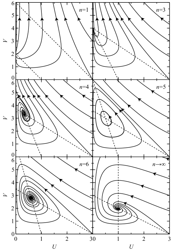
| Critical point | Eigenvalues | Eigenvectors | |||
|---|---|---|---|---|---|
Table A.1 shows the eigenvalues and eigenvectors for the critical points as functions of . The topologies of the HLEE in the – plane for the cases , , , , and are plotted in Fig. A.4. The origin is the first critical point. It is a saddle with solutions on the -axis approaching and those on the -axis escaping. Solutions near the origin move down and to the right in the – plane. There is a further critical point on each of the axes. On the -axis, is a saddle for all values of . It is stable along the -axis and unstable across it. This point coincides with the regular centre of realistic stellar models that was discussed previously. Along the -axis, is also a critical point. For it is a source and for a saddle. The intersection of the lines of horizontals and verticals is the final critical point . For each , . The character of these points varies with .
The behaviour of and distinguishes the topology of solutions into three regimes. For , is a pure source: it is unstable across and along the -axis. The point has and therefore does not feature in the first quadrant of the – plane but approaches the -axis from the left as . When , and co-incide. The point is marginally stable across the axis. For , and separate. is a saddle and a source, gradually moving towards its position at when . Fig. A.4 illustrates some features of the HLEE when . The lines of verticals and horizontals meet at , which has just appeared on the – plane at .
When , which separates the cases of finite and infinite polytropes, the – plane takes on a particular topology, illustrated in Fig. A.4. The polytrope is a straight line from to . The point is a centre, with solutions forming closed loops around it. The polytrope separates solutions that circulate around from those that go from to entirely above the polytrope. These solutions have zero mass at non-zero inner radius but, unlike the polytrope, have a finite outer radius.
As increases further becomes a spiral sink. Polytropes start at and spiral into (see Fig. A.4). There is an unstable solution that proceeds from to above which solutions extend to . As we also find and, in the limiting case of the isothermal sphere, all solutions ultimately spiral into because they cannot lie above the unstable solution.
We have been going around the workshop in the basement of the building of science. The light is dim, and we stumble sometimes. About us is confusion and mess which there has not been time to sweep away. The workers and their machines are enveloped in murkiness. But I think that something is being shaped here—perhaps something rather big. I do not quite know what it will be when it is completed and polished for the showroom. But we can look at the present designs and the novel tools that are being used in its manufacture; we can contemplate too the little successes which make us hopeful.
from The Expanding Universe,
Arthur S. Eddington, 1936