Measurement of the neutron $\bm{\beta}$-asymmetry parameter $\bm{A_{0}}$ with ultracold neutrons

Abstract

We present a detailed report of a measurement of the neutron $\beta$-asymmetry parameter $A_{0}$, the parity-violating angular correlation between the neutron spin and the decay electron momentum, performed with polarized ultracold neutrons (UCN). UCN were extracted from a pulsed spallation solid deuterium source and polarized via transport through a 7-T magnetic field. The polarized UCN were then transported through an adiabatic-fast-passage spin-flipper field region, prior to storage in a cylindrical decay volume situated within a 1-T $2\times 2\pi$ solenoidal spectrometer. The asymmetry was extracted from measurements of the decay electrons in multiwire proportional chamber and plastic scintillator detector packages located on both ends of the spectrometer. From an analysis of data acquired during runs in 2008 and 2009, we report $A_{0}=-0.11966\pm 0.00089~{}_{-0.00140}^{+0.00123}$, from which we extract a value for the ratio of the weak axial-vector and vector coupling constants of the nucleon, $\lambda=g_{A}/g_{V}=-1.27590\pm 0.00239~{}_{-0.00377}^{+0.00331}$. Complete details of the analysis are presented.

I Introduction

Precise measurements of neutron $\beta$-decay observables determine fundamental parameters of the weak interaction and contribute to tests of the Standard Model nico05 ; severijns06 ; abele08 ; nico09 ; dubbers11 ; severijns11 . Because the momentum transfer in neutron $\beta$-decay ($n\rightarrow p+e^{-}+\overline{\nu}_{e}+781.5$ keV) is small compared to the $W^{-}$ mass, the decay can be modeled as a four-fermion contact interaction with an amplitude under the Standard Model given by

$$\mathcal{M}=\frac{G_{F}V_{ud}}{\sqrt{2}}\langle p|J^{\mu}|n\rangle L_{\mu},$$ (1)

where $G_{F}$ is the Fermi weak coupling constant, $V_{ud}$ is the weak-quark-mixing CKM matrix element, and $L_{\mu}=\overline{u}_{e}\gamma_{\mu}(1-\gamma_{5})u_{\overline{\nu}}$ is the leptonic weak vector and axial-vector current. In its most general form, the hadronic weak vector and axial-vector ($V-A$) current includes six form factors goldberger58 ; weinberg58 ,

$$\langle p|J^{\mu}|n\rangle=\overline{u}_{p}\left[g_{V}(q^{2})\gamma^{\mu}-i\frac{g_{WM}(q^{2})}{2M}\sigma^{\mu\nu}q_{\nu}+\frac{g_{S}(q^{2})}{2M}q^{\mu}+g_{A}(q^{2})\gamma^{\mu}\gamma^{5}-i\frac{g_{T}(q^{2})}{2M}\sigma^{\mu\nu}\gamma_{5}q_{\nu}+\frac{g_{P}(q^{2})}{M}\gamma_{5}q^{\mu}\right]u_{n},$$ (2)

where $q$ is the four-momentum transfer; $M$ is the nucleon mass; and $g_{V}(q^{2})$, $g_{WM}(q^{2})$, $g_{S}(q^{2})$, $g_{A}(q^{2})$, $g_{T}(q^{2})$, and $g_{P}(q^{2})$ are the vector, weak magnetism, induced scalar, axial vector, induced tensor, and induced pseudoscalar form factors, respectively. In the limit of $q^{2}\rightarrow 0$, the hadronic weak current is dominated by the weak vector and axial vector coupling constants of the nucleon, defined to be the values of the vector and axial vector form factors at $q^{2}=0$, $g_{A}\equiv g_{A}(q^{2}=0)$ and $g_{V}\equiv g_{V}(q^{2}=0)$. Under the Conserved Vector Current (CVC) hypothesis of the Standard Model and the assumption of isospin symmetry, the vector coupling constant is $g_{V}=1$ (independent of the nuclear medium). Isospin-symmetry-breaking effects to the value of $g_{V}$ in neutron $\beta$-decay have been calculated in chiral perturbation theory, with the correction to $g_{V}$ found to be at a negligible $-4\times 10^{-5}$ level kaiser01 . Also per the CVC hypothesis, the weak magnetism coupling constant, $g_{WM}\equiv g_{WM}(q^{2}=0)$, which appears at recoil order in the vector current, is related to the proton and neutron anomalous magnetic moments by $g_{WM}=\kappa_{p}-\kappa_{n}$.

In contrast to the vector current, the axial-vector current is renormalized by the strong interaction such that the value of $g_{A}$ must be determined experimentally and also by lattice Quantum Chromodynamics (QCD) calculations. Any contribution from the induced pseudoscalar coupling constant, $g_{P}$, to neutron $\beta$-decay observables is expected to be negligibly small, with the contribution of $g_{P}$ to the energy spectrum calculated to be of order $m_{e}^{2}/ME_{e}\sim 10^{-4}$ holstein74 .

The two remaining terms, the induced scalar, $g_{S}(q^{2})$, in the vector current, and the induced tensor, $g_{T}(q^{2})$, in the axial-vector current, are termed second-class currents due to their transformation properties under $G$-parity. Under the requirement of $G$-parity symmetry, both $g_{S}(q^{2})=g_{T}(q^{2})=0$. However, $G$-parity symmetry is violated within the Standard Model due to differences in the $u$ and $d$ quarks’ charges and masses (i.e., isospin symmetry breaking effects). An estimate for $g_{T}$ including SU(3) breaking effects suggested $|g_{T}|$ in neutron $\beta$-decay to be $\lesssim 0.03$ donoghue82 , and an evaluation of $g_{T}/g_{A}$ using QCD sum rules found $g_{T}/g_{A}=-0.0152(53)$ shiomi96 . Finally, recent lattice QCD studies of SU(3) breaking in semi-leptonic decays find small, $\mathcal{O}(0.1)$, values for both $g_{S}(q^{2})$ and $g_{T}(q^{2})$ in neutron $\beta$-decay, but the results are statistically limited and consistent with zero at 1–2 standard deviations sasaki09 . However, despite these hints for non-zero values of these second-class currents, their contributions to neutron $\beta$-decay observables are again expected to be negligibly small, as they also appear at order $m_{e}^{2}/ME_{e}\sim 10^{-4}$ in the energy spectrum holstein74 .

Therefore, under the assumption that any such contributions from $g_{P}$, $g_{S}$, and $g_{T}$ are negligibly small relative to the current level of experimental precision, it is clear that a description of neutron $\beta$-decay under the CVC hypothesis of the Standard Model requires the specification of only two parameters, $V_{ud}$ and $g_{A}$, given the high precision results for $G_{F}$ achieved in muon decay webber11 . Both $V_{ud}$ and $g_{A}$ can be accessed via measurements of two different types of neutron $\beta$-decay observables: the lifetime, and angular correlation coefficients in polarized and unpolarized $\beta$-decay. The first of these, the lifetime, as calculated from the amplitude and integration over the allowed phase space, is of the form czarnecki04

$$\frac{1}{\tau_{n}}=\frac{G_{F}^{2}m_{e}^{5}}{2\pi^{3}}V_{ud}^{2}\left(1+3\lambda^{2}\right)f\left(1+\text{RC}\right),$$ (3)

where $m_{e}$ is the electron mass and the parameter $\lambda$ is defined to be the ratio of the axial vector and vector coupling constants, $\lambda\equiv g_{A}/g_{V}$. The numerical value for the phase space factor of $f=1.6887$ czarnecki04 includes corrections for the Fermi function, the finite nucleon mass, the finite nucleon radius, and the effect of recoil on the Fermi function. The factor $(1+\text{RC})$ denotes the total effect of all electroweak radiative corrections, including the $\mathcal{O}(\alpha)$ outer (long-distance loop and bremsstrahlung effects) and inner (short distance, including axial-vector-current, loop effects) radiative corrections; an $\mathcal{O}(\alpha^{2})$ correction resulting from factorization of the Fermi function; and $\mathcal{O}(\alpha^{2})$ leading-log and next-to-leading-log corrections (for lepton and quark loop insertions in the photon propagator) czarnecki04 . The total electroweak radiative correction has been calculated to be $(1+\text{RC})=1.0390\pm 0.0004$ marciano06 where the $\pm 0.0004$ uncertainty was reduced by a factor of two (from its previous value of $\pm 0.0008$ czarnecki04 ) after the development of a new method for calculating hadronic effects in the matching of long- and short-distance contributions to axial-vector current loop effects (primarily from the $\gamma W$ box diagram).

The second type of observable, angular correlation coefficients, parametrize the angular correlations between the momenta of the decay products and the spin of the initial-state neutron. In general, the directional distribution of the electron and antineutrino momenta and the electron energy in polarized $\beta$-decay is of the form jackson57

$$\displaystyle{\frac{d\Gamma}{dE_{e}d\Omega_{e}d\Omega_{\nu}}}\propto p_{e}E_{e}(E_{0}-E_{e})^{2}$$

$$~{}~{}\times\left[1+b\frac{m_{e}}{E_{e}}+a\frac{\vec{p}_{e}\cdot\vec{p}_{\nu}}{E_{e}E_{\nu}}\right.$$

$$~{}~{}~{}~{}~{}~{}~{}\left.+~{}\langle\vec{\sigma}_{n}\rangle\cdot\left(A\frac{\vec{p}_{e}}{E_{e}}+B\frac{\vec{p}_{\nu}}{E_{\nu}}+D\frac{\vec{p}_{e}\times\vec{p}_{\nu}}{E_{e}E_{\nu}}\right)\right],$$ (4)

where $E_{e}$ ($E_{\nu}$) and $\vec{p}_{e}$ ($\vec{p}_{\nu}$) denote, respectively, the electron’s (antineutrino’s) total energy and momentum; $E_{0}$ ($=781.5$ keV + $m_{e}$) is the electron endpoint energy; and $\langle\vec{\sigma}_{n}\rangle$ is the neutron polarization. The angular correlation coefficients $a$ ($e$-$\overline{\nu}_{e}$-asymmetry), $A$ ($\beta$-asymmetry), and $B$ ($\overline{\nu}_{e}$-asymmetry) are, to lowest order, functions only of $\lambda$ where, under a $\lambda<0$ sign convention,

$$a_{0}=\frac{1-\lambda^{2}}{1+3\lambda^{2}},~{}~{}~{}A_{0}=-2\frac{\lambda(\lambda+1)}{1+3\lambda^{2}},~{}~{}~{}B_{0}=2\frac{\lambda(\lambda-1)}{1+3\lambda^{2}}.$$

(5)

The contributions of terms in Eq. (4) proportional to the Fierz interference term $b$ and the time-reversal-odd triple-correlation-coefficient $D$ are at recoil order for Standard Model interactions holstein74 ; bhattacharya12 ; callan67 ; ando09 , and are negligible at the current level of experimental precision. Note that to our knowledge, there are no published direct measurements of $b$ in neutron $\beta$-decay.

As already noted, at lowest order $a_{0}$, $A_{0}$, and $B_{0}$ are functions only of $\lambda$. However, recoil-order corrections, including the effects of weak magnetism and $g_{V}$-$g_{A}$ interference, introduce energy-dependent corrections to the asymmetry, and are of $\mathcal{O}$(1%) for $a$ and $A$ holstein74 ; wilkinson82 ; gardner01 and $\mathcal{O}$(0.1%) for $B$ gluck98 . For $A$, the recoil-order corrections are of the explicit functional form holstein74 ; wilkinson82 ; gardner01

$$A=A_{0}+A_{1}\frac{\epsilon}{Rx}+A_{2}R+A_{3}Rx,$$ (6)

where $R=E_{0}/M$, $\epsilon=(m_{e}/M)^{2}$, $x=E_{e}/E_{0}$, and the $A_{i}$ ($i=1,2,3$) coefficients are functions only of $\lambda$ and $g_{WM}$ (assuming $g_{S}=g_{T}=0$, and negligible contributions from $g_{P}$). Under these assumptions, $A_{1}=-0.3054$, $A_{2}=0.7454$, and $A_{3}=-3.0395$. Note that the $q^{2}$ dependence of the form factors does not appear until next-to-leading recoil order gardner01 .

In addition to the above recoil-order corrections, there is a small energy-dependent radiative correction (for virtual and bremsstrahlung processes) to polarized asymmetries, resulting in a $\mathcal{O}(0.1\%)$ correction to $A$ shann71 ; gluck92 . After application of these recoil-order and radiative corrections, a value for $\lambda$ can be extracted from $a_{0}$, $A_{0}$, and $B_{0}$. Note, however, that for a given (relative) statistical precision, the sensitivity of $A_{0}$ to $\lambda$ is slightly higher than that of $a_{0}$, and a factor of $\sim 8$ greater than that of $B_{0}$, where at leading order the relative uncertainties compare as

$$\frac{\delta|\lambda|}{|\lambda|}\approx 0.24\frac{\delta|A_{0}|}{|A_{0}|}\approx 0.27\frac{\delta|a_{0}|}{|a_{0}|}\approx 2.0\frac{\delta|B_{0}|}{|B_{0}|}.$$ (7)

Thus, measurements of the angular correlation coefficients determine a value for $\lambda$ (or $g_{A}$, assuming $g_{V}=1$ under the CVC hypothesis), a fundamental parameter in the nucleon weak current. A precise value for $g_{A}$ is also important in many other contexts. In hadronic physics studies of the spin structure of the nucleon filippone02 ; bass05 , the Bjorken sum rule relates the difference in the first moments of the proton and neutron spin-dependent $g_{1}$ structure functions (i.e., isovector channel), as probed in polarized deep inelastic electron scattering, to $g_{A}$. In QCD, the assumption of a partially conserved axial-vector current (PCAC), valid in the limit of a massless pion (identified as the Goldstone boson of the spontaneously broken chiral symmetry), leads to the Goldberger-Treiman relation goldberger58 , relating the value of $g_{A}$ to the pion decay constant $f_{\pi}$, the weak pion-nucleon-nucleon coupling constant $g_{\pi NN}$, and the nucleon mass. The value of $g_{A}$ is also important in astrophysical processes, including calculations of solar fusion cross sections and rates, in particular, of the $pp$ fusion reaction, impacting the solar neutrino flux for this process adelberger11 . High-precision experimental results for $g_{A}$ also serve as an important benchmark for theoretical calculations of $g_{A}$, both in fundamental lattice QCD calculations yamazaki08 and in relativistic constituent quark model calculations choi10 . A precise value for $g_{A}$ is also important as a phenomenological input parameter (together with other low energy constants, such as the pion decay constant $f_{\pi}$, the nucleon mass, etc.) to effective field theory calculations involving the axial vector current gockeler05 .

Although not a fundamental weak interaction parameter by itself, a precise value for the lifetime is important for Big Bang Nucleosynthesis calculations, impacting the neutron-to-proton ratio and hence the primordial ⁴He abundance at the time of freeze-out, when the weak reaction rate became less than the Hubble expansion rate mathews05 . The value of the lifetime is also important for the interpretation of data from neutrino oscillation experiments employing antineutrinos from reactors mention11 , which typically search for the reaction $\overline{\nu}_{e}+p\rightarrow e^{+}+n$ in detectors. The cross section for this reaction is inversely proportional to the neutron lifetime; therefore, an accurate and precise experimental value for the lifetime is needed for an interpretation of measured detector antineutrino reaction rates in terms of the underlying neutrino oscillation physics.

Measurements of the lifetime and a value for $\lambda$ from measurements of angular correlation coefficients permit the extraction of a value for $V_{ud}$ solely from neutron $\beta$-decay observables according to Eq. (3). Although a value for $V_{ud}$ from neutron $\beta$-decay pdg is not yet competitive with the definitive value deduced from measurements of $ft$ values in superallowed $0^{+}\rightarrow 0^{+}$ nuclear $\beta$-decay towner10 , the appeal of such an extraction is that it does not require corrections for isospin-symmetry-breaking and nuclear-structure effects. Ultimately, when the precision on a neutron-based value for $V_{ud}$ approaches the precision of the $0^{+}\rightarrow 0^{+}$ result, the two values must agree in the absence of new physics. However, given that the neutron-based value for $V_{ud}$ is not yet competitive, one can treat the $0^{+}\rightarrow 0^{+}$ value for $V_{ud}$ as a fixed input parameter, and instead perform a robust test of the consistency of the various measured neutron $\beta$-decay observables under the Standard Model. In particular, results for $g_{A}$ extracted from correlation coefficient measurements can then be directly compared with results from measurements of the neutron lifetime $\tau_{n}$.

Finally, measurements of the angular correlation coefficients themselves are sensitive to beyond-the-Standard-Model physics, such as scalar and tensor interactions gudkov06 ; konrad10 ; bhattacharya12 . With the projected improvements to the experimental precision in future years, neutron $\beta$-decay measurements will be sensitive to any such sources of new physics at energy scales rivaling those probed directly at the Large Hadron Collider bhattacharya12 .

Table 1: Summary of published measurements of the neutron $\beta$-asymmetry parameter $A_{0}$. The error on the average has been increased by a factor of $\sqrt{\chi^{2}/\nu}=2.47$.

Experiment	Years Published	Type	Polarization	$A_{0}$ Result	Notes
PERKEO bopp86	1986	cold neutron beam	$0.974\pm 0.005$	$-0.1146\pm 0.0019$
PNPI erozolimskii91 ; yerozolimsky97	1991, 1997	cold neutron beam	$0.770\pm 0.007$	$-0.1135\pm 0.0014$
ILL-TPC schreckenbach95 ; liaud97	1995, 1997	cold neutron beam	$0.981\pm 0.003$	$-0.1160\pm 0.0015$
PERKEO II abele97 ; abele02	1997, 2002	cold neutron beam	$0.989\pm 0.003$	$-0.1189\pm 0.0007$
UCNA pattie09 ; liu10 , this work	2009, 2010	stored ultracold neutrons	$1.0^{+0}_{-0.0052}$	$-0.11966\pm 0.00089^{+0.00123}_{-0.00140}$
PERKEO II mund12	2012	cold neutron beam	$0.997\pm 0.001$	$-0.11996\pm 0.00058$
Current Average Value: $A_{0}=-0.11846\pm 0.00104$ ($\chi^{2}/\nu=24.35/4$)

The remainder of this article is organized as follows. In Section II, we summarize the current status of measurements of $A_{0}$. We then outline the experimental motivation for a measurement of $A_{0}$ with ultracold neutrons in Section III, and then present a detailed description of the UCNA (“Ultracold Neutron Asymmetry”) Experiment pattie09 ; liu10 at the Los Alamos National Laboratory. Our measurement procedures and experimental geometrical configurations are reported in Section IV. Results from our calibration and analysis procedures are discussed in Section V. Details of our procedure for the extraction of asymmetries are presented in Section VI, and the corrections to measured asymmetries for various systematic effects are discussed in Section VII. Systematic uncertainties are summarized in Section VIII, and our final results for $A_{0}$ are then reported in Section IX. We then conclude with a brief summary of the physics impact of our work in Section X. The data presented here were obtained during data-taking runs in 2008–2009 and published rapidly in 2010 liu10 ; in this article we provide a more detailed account of the experiment and analysis procedures.

II Status of Measurements of $\bm{A_{0}}$

The current status of published results bopp86 ; erozolimskii91 ; yerozolimsky97 ; schreckenbach95 ; liaud97 ; abele97 ; abele02 ; pattie09 ; liu10 ; mund12 for the neutron $\beta$-asymmetry parameter $A_{0}$ is summarized in Table 1 and shown in Fig. 1. Other than the UCNA Experiment, all of the experiments have been performed with beams of polarized cold neutrons, with reported values for the polarization ranging from $0.770\pm 0.007$ erozolimskii91 ; yerozolimsky97 to $0.997\pm 0.001$ mund12 . Magnetic solenoidal spectrometers providing $2\times 2\pi$ solid angle acceptance for detection of the decay electrons were employed in the PERKEO bopp86 and PERKEO II abele97 ; abele02 ; mund12 experiments at the Institut Laue-Langevin (ILL). In contrast, the solid angle was defined by the geometric acceptance in an experiment at the Petersburg Nuclear Physics Institute (PNPI) erozolimskii91 ; yerozolimsky97 in which the decay electrons and protons were detected in coincidence in detectors surrounding the beam decay region, and in an experiment at the ILL schreckenbach95 ; liaud97 which utilized a time projection chamber for reconstruction of the electron track.

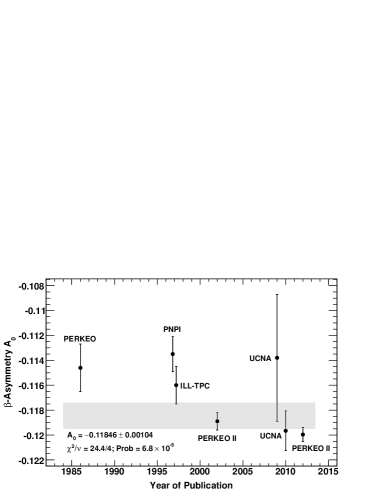
Figure 1: Results from measurements of the $\beta$-asymmetry parameter $A_{0}$ bopp86 ; erozolimskii91 ; yerozolimsky97 ; schreckenbach95 ; liaud97 ; abele97 ; abele02 ; pattie09 ; liu10 . The band ($\pm 1\sigma$) indicates the current world average value of $A_{0}=-0.11846\pm 0.00104$.

The current world average value for $A_{0}=-0.11846\pm 0.00104$ includes the most recent PERKEO II result mund12 , but excludes the UCNA proof-of-principle result pattie09 . Note that the current error bar of $\pm 0.00104$ includes the Particle Data Group’s $\sqrt{\chi^{2}/\nu}$ scaling pdg . The need for this expanded error bar suggests an incomplete assessment of the systematic errors in one or more of the cold-neutron-based experiments.

III UCNA Experiment

III.1 Overview of Experiment

The UCNA Experiment, installed in Area B of the Los Alamos Neutron Science Center (LANSCE) at the Los Alamos National Laboratory (LANL), was designed to perform the first-ever measurement of the neutron $\beta$-asymmetry parameter with ultracold neutrons (UCN), and to-date is the only experimental measurement of any neutron $\beta$-decay angular correlation coefficient performed with ultracold neutrons (UCN). UCN are defined to be neutrons with kinetic energies sufficiently low ($\lesssim 335$ neV, corresponding to speeds $\lesssim 8$ m s^-1) such that they undergo total external reflection at any angle of incidence from an effective potential barrier (a volume average of Fermi potentials $V_{\text{Fermi}}$) at the surfaces of certain materials ucn_book . Thus, UCN can be stored in material-walled vessels, whereas cold neutrons (kinetic energies 0.05–25 meV, speeds 100–2200 m s^-1) must be transported along neutron guides at reflection angles less than the guide critical angle, resulting in short residency times in an apparatus.

Figure 2: Schematic diagram (not to scale) of the primary components of the UCNA Experiment’s $\beta$-asymmetry measurement. The top panel depicts the layout of the 7.0-Tesla polarizing magnet and AFP spin-flipper, the 1.0-Tesla spectrometer, the decay trap, and the electron detectors. The bottom panel depicts the UCN source and shielding, the layout of the UCN transport guides, the location of the UCN gate valve, the location of the UCN switcher, the locations of all the magnets, and the locations of all the UCN monitor detectors. All of these components are described in detail later in the text. [Note that during our data-taking runs in 2009, the (bare) Cu UCN guides located between the spin-flipper and the entrance to the decay trap (as depicted in the top panel) were replaced with diamondlike carbon-coated Cu guides; see Section IV.2 for details.]

A schematic diagram of the UCNA Experiment is shown in Fig. 2, and the basic principle of the experiment is as follows. Spallation neutrons resulting from the interaction of a pulsed (typically 0.2 Hz) 800 MeV proton beam with a tungsten target were moderated in cold polyethylene to the cold neutron regime, and then downscattered to the UCN regime in a solid deuterium (SD₂) crystal. The UCN were then transported along a series of UCN guides through a 7.0-Tesla solenoidal polarizing magnet, where the spin-dependent $-\vec{\mu}\cdot\vec{B}$ potential ($\pm 60$ neV T^-1) served as a spin-state selector for magnetic moments $\vec{\mu}$ oriented parallel to the direction of the longitudinal magnetic field $\vec{B}$. The polarized UCN were then transported along non-magnetic UCN guides through an adiabatic-fast-passage (AFP) spin-flipper 1.0-Tesla field region, used to prepare UCN with spins either parallel or anti-parallel to the magnetic field. The UCN were then directed to the center of a 12.4-cm diameter, 3-m long cylidrical decay storage volume located within the warm bore of a 1.0-T solenoidal spectrometer. Emitted $\beta$-decay electrons then spiraled (with a maximum Larmor diameter of 7.76 mm for 782 keV endpoint electrons emitted perpendicular to the 1.0-T field) along the magnetic field lines towards one of two electron detectors located on both ends of the spectrometer.

In principle, the $\beta$-asymmetry $A$ can be extracted from measurement of the $W(\theta)\propto(1+P_{n}A\beta\cos\theta)$ angular distribution by forming an energy-dependent “measured asymmetry”, $A_{\text{meas}}(E_{e})$, of the detectors’ (background-subtracted) count rates,

$$A_{\text{meas}}(E_{e})=\frac{r_{1}(E_{e})-r_{2}(E_{e})}{r_{1}(E_{e})+r_{2}(E_{e})}=P_{n}A\beta\langle\cos\theta\rangle,$$ (8)

where $r_{1(2)}(E_{e})$ denote the energy-dependent count rates observed in the two detectors, $P_{n}$ denotes the neutron polarization, $\beta$ denotes the electron velocity in units of $c$, and $\langle\cos\theta\rangle$ is the average value of $\cos\theta$ integrated over the detectors’ angular acceptance for that particular value of $E_{e}$. Note that for nominal values of $P_{n}\sim 1$, $A\sim-0.12$, $\beta\sim 0.75$, and $\langle\cos\theta\rangle\sim 1/2$, the experimental measured asymmetry is of order $|A_{\text{meas}}|\sim 0.04$.

In practice, the asymmetry is extracted from ratios of the two detectors’ energy-dependent count rates for the two neutron spin states with polarizations oriented parallel and anti-parallel to the magnetic field via a “super-ratio” technique. Here, the super-ratio, $R$, is defined in terms of the measured energy-dependent detector count rates for the two spin states, $r_{1(2)}^{+(-)}(E_{e})$, to be

$$R=\frac{r_{1}^{-}(E_{e})\cdot r_{2}^{+}(E_{e})}{r_{1}^{+}(E_{e})\cdot r_{2}^{-}(E_{e})},$$ (9)

with the energy-dependent measured asymmetry, $A_{\text{meas}}(E_{e})$, then calculated from the super-ratio according to

$$A_{\text{meas}}(E_{e})=\frac{1-\sqrt{R}}{1+\sqrt{R}}=P_{n}A\beta\langle\cos\theta\rangle.$$ (10)

The merit of this super-ratio technique is that effects due to differences in the two detectors’ efficiencies and spin-dependent differences in the efficiencies for transport of the two UCN spin states into the spectrometer cancel to first order. In a binned analysis, energy-dependent detection efficiencies also largely cancel in the super-ratio, and are negligible for the energy bin sizes used in this work.

The motivation for the development of the UCNA Experiment was several-fold. First, the use of UCN in a neutron $\beta$-asymmetry experiment controls key neutron-related systematic corrections and uncertainties, including the neutron polarization and neutron-generated backgrounds. As discussed in detail later in this article, the polarization has been demonstrated to be $>99.48$% at the 68% C.L., with the precision, at present, limited only by statistics. Further, neutron-generated backgrounds have been constrained to be negligible, a direct result of the relatively small number of neutrons present in the apparatus at any time, the small probability for their capture and subsequent generation of accompanying irreducible gamma ray backgrounds, and the fact that nearly all of the neutrons present in the apparatus are located within the spectrometer’s decay volume. In the UCNA Experiment, a relatively large fraction, $\sim 1/40$, of the UCN stored in the decay volume contribute to the measured decay rate, whereas in cold neutron beam experiments typically only $\sim 1/10^{7}$ of the neutrons passing through the apparatus contribute to the decay rate abele97 . Therefore, control of neutron-generated backgrounds is expected to be intrinsically more challenging in cold neutron beam experiments.

Second, as described in detail elsewhere ito07 ; plaster08 , the electron detector system developed for the UCNA Experiment, consisting of a low-pressure multiwire proportional chamber (MWPC) backed by a plastic scintillator, provides position sensitivity, suppresses ambient gamma-ray backgrounds, and permits the reconstruction of low-energy-deposition electron backscattering events. The UCNA Experiment is the first neutron $\beta$-asymmetry experiment to employ a MWPC, providing the experiment with two critical advantages. First, the position information permits the definition of a fiducial volume on an event-by-event basis. Second, the position information also permits for an event-by-event correction for the scintillator’s position-dependent energy response.

We now provide a more detailed description of the primary components of the UCNA Experiment.

III.2 UCN Source and Guide Transport System

A detailed description of the design principles and performance of the LANL SD₂ UCN source is given elsewhere morris02 ; saunders04 ; saunders11 ; therefore, we provide only a brief description here. Protons from the 800 MeV LANSCE accelerator were delivered in pulsed mode at a repetition rate of 0.2 Hz to a tungsten spallation target, which was surrounded by a room-temperature beryllium reflector. With the spallation target operated in this pulsed mode, prompt beam related backgrounds can be eliminated with simple timing cuts, with negligible loss of duty factor for the $\beta$-decay measurements performed with the UCN stored in the electron spectrometer. The spallation neutrons were moderated in cold-helium-gas-cooled polyethylene (maintained at a temperature of $\sim 150$ K for time-averaged proton beam currents of 5.8 $\mu$A) located between the tungsten target and the beryllium reflector. The moderated cold neutrons were then downscattered to the UCN regime in a $\sim 2$ L cylindrical volume of ortho-state SD₂ liu00 ; liu03 embedded at the bottom of a vertically-oriented cylindrical liquid-helium-cooled aluminum cryostat coated with ⁵⁸Ni, presenting a nominal effective potential of 342 neV to the emerging UCN flux. The SD₂ was maintained at temperatures $<10$ K during the proton beam pulses on the spallation target. A butterfly-style “flapper” valve coated with ⁵⁸Ni was located immediately above the SD₂ volume. This “flapper” valve opened and subsequently closed (with opening and closing response times of about 0.1 s) with each proton pulse, in order to increase the storage lifetime of the UCN in the volume of the source above the SD₂ volume. A typical UCN lifetime with the flapper open was $9.6\pm 0.2$ s, whereas the lifetime with the flapper closed was $39.4\pm 0.1$ s. The flapper leads to a corresponding increase in the UCN density.

The UCN were then extracted from the source along horizontally-oriented 10.16-cm diameter stainless steel guides (presenting a nominal potential of 189 neV) through the biological shielding surrounding the source and out into the experimental area. As shown in Fig. 2, this system of guides through the biological shielding included two $45^{\circ}$ bends to eliminate neutrons with kinetic energies above the stainless steel guide potential. The maximum UCN density at the biological shield exit that we have obtained is $52\pm 9$ cm^-3 saunders11 , but for this work (runs in 2008–2009) typical densities were $\sim 35\pm 6$ cm^-3. After exiting the biological shield, the UCN were transported along stainless steel guides through a gate valve, which served to separate the UCN source from the experiment, thus permitting measurements of backgrounds in the electron spectrometer detectors with the proton beam still operating in its normal pulsed mode, but no accompanying UCN transport to the spectrometer. A 6.0-T superconducting solenoidal pre-polarizing magnet (PPM) was located immediately downstream of this gate valve. The PPM was included in the experiment design in order to minimize UCN transport losses through a thin (0.0254-mm thick) Zr foil which served to separate the vacuum in the SD₂ source from the downstream vacuum in the remainder of the experiment. Note that the UCN population was polarized after transport through the PPM’s longitudinal magnetic field.

To preserve this initial polarization, 10.16-cm diameter electropolished Cu guides (nominal potential of 168 neV) were installed downstream of the PPM magnet. The UCN were then transported along these guides through a “switcher” valve, which allowed the downstream guides comprising the $\beta$-asymmetry measurement to be connected to either the upstream guides from the UCN source, or to a ³He UCN detector morris09 used, as described later, for measurements of the depolarized population. These electropolished Cu guides then transported the UCN through the primary 7.0-T polarizing magnet (called the AFP magnet). A 100-cm long quartz guide section coated with diamondlike carbon (DLC) mammei-thesis passed through the center of a resonant (1.0-T) “bird-cage” r.f. cavity holley_afp , used for adiabatic fast passage (AFP) spin-flipping of the UCN.

Downstream of this DLC-coated quartz guide, another section of 10.16-cm diameter Cu guide transitioned to a 7-cm (vertical) $\times$ 4-cm (horizontal) rectangular Cu guide, which transported the UCN through a horizontal penetration in the 1.0-T solenoidal electron spectrometer coil into the decay trap. Permanent magnets were attached to the outer surfaces of the rectangular guide in order to suppress Majorana spin-reorientations vladimirski61 of neutrons passing through “field zeros” in the 1.0-T solenoidal spectrometer’s field.

The UCN rate along the transport guide system was monitored with ³He UCN detectors morris09 at two key locations: at the gate valve (for monitoring of the SD₂ source performance), and slightly downstream of the APF spin flipper (for monitoring of the AFP spin-flipping efficiency). These ³He UCN detectors were coupled to the guide system via small (0.64-cm diameter) holes in the bottom of the guides. Note that the UCN density in the spectrometer for the spin-flipped state was smaller than that for the unflipped state, because of losses (after the 2.0-T $\vec{\mu}\cdot\vec{B}$ energy boost associated with the spin flip) in the transport guides located between the AFP spin-flip region and the electron spectrometer. The measured $\beta$-decay rates for the spin-flipped state were $\sim 25$% smaller than those for the non-spin-flipped state.

The maximum neutron $\beta$-decay rates measured in the spectrometer during the 2008–2009 runs correspond to a stored density of approximately 1 cm^-3 in the decay trap. Major sources of loss are transport through the high field regions in the PPM and in the AFP magnet. The transport though the PPM is about 25%. Approximately half of the loss is due to polarization of the neutrons, and the other half is due to UCN absorption in the Zr foil and non-specular scattering on the UCN guide walls in the high field region of the magnet which leads to enhanced wall losses. There is an approximate 15% loss in UCN density in the transition from the stainless steel to the copper guides because of the lower Fermi potential of the copper. Transmission through the AFP magnet is about 60%, again due to non-specular scattering in the high field region. There is a 50% loss in density in loading the decay trap because the loading time (which is determined by the aperture of the above-described 7-cm $\times$ 4-cm rectangular guide) and decay trap lifetime are nearly the same. Finally, there is an approximate factor of two loss in the transport from the biological shield exit to the decay trap due to guide losses. (The typical loss per bounce in the guide system is $3\times 10^{-4}$ which is dominated by gaps in the guide couplings.) Thus, all of these factors combined account for the reduction in the UCN density from its intial value of $\sim 35$ cm^-3 at the biological shield exist to $\sim 1$ cm^-3 in the spectrometer decay trap during runs in 2008–2009.

III.3 Decay Trap Geometry

The decay trap consisted of a 300-cm long, 12.4-cm diameter electropolished Cu tube situated along the warm bore axis of the 1.0-T solenoidal electron spectrometer. The vacuum pressure in the UCN guides downstream of the Zr foil in the PPM and in the decay trap was typically $\sim 10^{-5}$ Torr. The ends of the decay trap were closed off with variable thickness mylar end-cap foils, whose inside surfaces were coated with 300 nm of Be (nominal 252 neV potential) which served to increase the UCN storage time in the decay trap (and, hence, the $\beta$-decay rate). An additional important feature of the end-cap foils is that they eliminated the possibility for neutron $\beta$-decay events in the region of the spectrometer where the field is expanded from 1.0-T to 0.6-T (discussed later in Section III.5.1). Collimators with inner radii of 5.84 cm mounted on the two ends of the decay trap suppressed events originating near the decay trap walls and also functioned as mounts for the end-cap foils. As discussed in more detail later, the thicknesses of the mylar end-cap foils were varied from 0.7 $\mu$m to 13.2 $\mu$m to study key systematics related to electron energy loss in, and backscattering from, these foils.

The UCN density in the decay trap was monitored by a ³He UCN detector coupled to a small (0.64-cm diameter) hole in the bottom of the decay trap center, as indicated schematically in Fig. 2.

III.4 Polarization and Spin Flipping System

A detailed description of the 7.0 T polarizing magnet and the AFP spin-flip system is given elsewhere holley_afp ; therefore, we provide only a brief description of this system here.

The solenoidal superconducting magnet which serves as the primary UCN polarizer (the AFP magnet) and provides the requisite environment for an adiabatic fast-passage (AFP) spin flipper was designed by American Magnetics using a cryostat supplied by Ability Engineering. It possesses a 194.9 cm long, 12.7 cm diameter warm bore and provides both a peak field of 7.0-T near the entrance as well as a 44.5-cm long precision gradient spin-flip region with an average field of 1.0 T, chosen to reduce neutron spectral differences between the flipped and unflipped spin states in the electron spectrometer decay trap volume. When energized to 96.45 A, the main coil of this magnet produces both the maximum polarizing field as well as the 1 T field, with an average gradient of $6\times 10^{-5}$ T cm^-1 through the latter. Ten superconducting shim coils centered on the uniform field region and spaced every 5.1 cm provide the ability to further tailor the uniform field in order to optimize performance of the spin flipper.

Due to the high field in the spin flip region, the spin flipper was constructed using an efficient high-pass birdcage resonant cavity geometry holley_afp . For the UCNA Experiment, this configuration was realized with eight Cu tubes (rungs) arranged in a cylindrical geometry and connected at the top by 820 pF American Technical Ceramics chip capacitors and at the bottom by a sliding Cu tuning ring whose position determined the inductance presented by the Cu tubes. When excited by an r.f. signal such a geometry is resonant, with the fundamental mode corresponding to a discretized sinusoidal distribution of current in the rungs. This current distribution provides a transverse r.f. field, one rotating component of which is utilized for AFP spin flipping, providing efficient spin reversal over a wide band of neutron speeds holley_afp . The specific operation frequency was adjusted by moving the tuning ring, and the cavity formed after tuning the spin flipper to operate at $\sim 28$ MHz was $\sim 15$ cm long (8.74 cm diameter), coaxial with a 7 cm diameter DLC-coated quartz UCN guide.

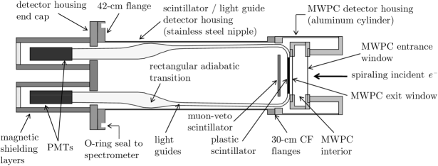
Figure 3: Schematic diagram (not to scale) of the MWPC and plastic scintillator electron detector package.

The UCNA spin flipper was typically operated with 40 W of input power, which necessitated an impedance-matching system comprised of a calculated length of drive line and three Jennings vacuum variable capacitors. Water cooling was also required, and was accomplished by flowing chilled, filtered tap water serially through the rungs. In order to provide for stable electrical operation and to prevent r.f. radiation from inducing noise elsewhere in the experiment, the birdcage cavity was driven in a balanced mode and electrically shielded by a grounded Al cylindrical enclosure which also provided a vacuum seal around the DLC-coated quartz guide. The interior of this enclosure connected through four bellows to the outside of the AFP magnet so that the actual r.f. cavity remained at atmosphere while the AFP magnet bore and the guide system were under vacuum. This arrangement also provided feedthroughs for the r.f. drive line, water cooling lines, an RTD temperature sensor, and an r.f. field sensor loop.

Initial characterization of the spin flipper was performed in a crossed polarizer analyzer geometry as described in holley_afp , which determined the average spin flip efficiency to be $0.9985\pm 0.0004$. During the actual running of the UCNA experiment during the years 2008–2009, tuning of the spin flipper, as well as run-to-run monitoring of its performance, was accomplished using a ³He UCN monitor located just downstream of the AFP magnet, $\sim 1$ m below a $\sim 0.64$ cm hole in the bottom of the guide (the location of this UCN monitor is indicated schematically in Fig. 2). This detector had a magnetized Fe foil covering the detector acceptance which provided for spin state selection.

III.5 Electron Spectrometer System

The electron spectrometer system, consisting of a 1.0-T superconducting solenoidal magnet and a multiwire proportional chamber (MWPC) and plastic scintillator electron detector package, is described in detail elsewhere ito07 ; plaster08 . Nevertheless, for completeness, we discuss the primary components of this system here. As described below, the electron spectrometer system was designed both to suppress the total electron backscattering fraction and to reconstruct low-energy-deposition backscattering events. The primary components of the two identical MWPC and plastic scintillator detector packages are shown in Fig. 3.

III.5.1 1.0-T Superconducting Solenoidal Magnet

The spectrometer magnet plaster08 is a warm-bore 35-cm diameter, 4.5-m long superconducting solenoid (hereafter, SCS magnet). The coil, which was designed and fabricated by American Magnetics, Inc., consists of a main coil winding with a single persistence heater switch, 28 shim coil windings (each with individual persistence heater switches), and three rectangular 7-cm $\times$ 4-cm radial penetrations (two providing horizontal access, and one providing vertical access, to the warm bore). These penetrations are located at the center of the coil. The magnet’s 1600-L capacity liquid helium cryostat was designed and fabricated by Meyer Tool and Manufacturing, Inc. The magnet’s full energized field strength of 1.0 T requires a current of 124 A in the main coil winding. Note that the magnet’s shim coils were not energized during the data-taking runs reported in this article.

An important feature of the SCS magnet design was that the field is expanded, as indicated schematically in Fig. 2, from 1.0 T in the decay trap region to 0.6 T at the location of the MWPC and plastic scintillator electron detectors, to suppress large-pitch-angle backscattering. In particular, the field-expansion ratio of 0.6 maps pitch angles of $90^{\circ}$ in the 1.0-T region to pitch angles of $51^{\circ}$ in the 0.6-T region. Another important feature of the magnet design concerned the field uniformity in the decay trap region. Electrons emitted with momentum $p_{0}=(p_{\perp,0}^{2}+p_{\parallel,0}^{2})^{1/2}$, with $p_{\perp,0}$ ($p_{\parallel,0}$) the initial transverse (longitudinal) momentum component, in some local field $B_{0}$ will be reflected from field regions $B$ if $B>B_{\text{crit}}\equiv(p_{0}^{2}/p_{\perp,0}^{2})B_{0}$, thus contributing to a false asymmetry. By this same process, electrons emitted at large pitch angles in the vicinity of a local field minimum will be trapped.

The SCS field profile measured during the data-taking period reported in this article is shown in Fig. 4. As can seen there, the field was uniform to the level of $5\times 10^{-3}$ over the decay trap length, but included a $\sim 0.005$ T “dip” near the center of the decay trap. Note that the field uniformity shown here was degraded from that originally published in plaster08 ; this was the result of damage to the shim coil persistence heater switches during multiple magnet quenches. The impact of this field non-uniformity on the measured asymmetry is discussed later in this article.

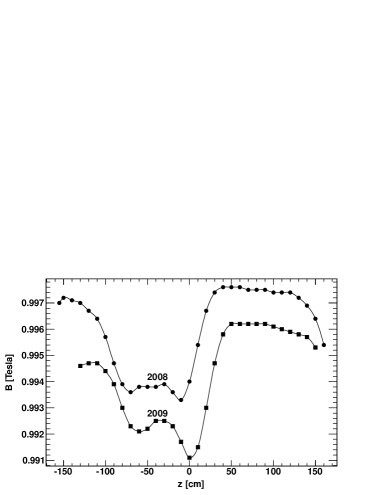
Figure 4: Measured SCS field profile during 2008 (circles) and 2009 (squares). The two data sets have been offset for purposes of clarity. The coordinate system is such that the 300-cm long decay trap is centered at $z=0$.

III.5.2 Multiwire Proportional Chamber

Some of the most important features of the MWPC ito07 are as follows. First, because an MWPC is relatively insensitive to gamma rays, requiring a coincidence between the MWPC and the scintillator greatly suppressed gamma-ray backgrounds, a dominant background source in previous experiments (see, e.g., background spectrum in abele97 ).

Second, the MWPC permitted reconstruction of an event’s transverse $(x,y)$ position. This permitted the definition of a fiducial volume and the subsequent rejection of events occurring near the decay trap walls. Such electrons can scatter from the decay trap walls, leading to a distortion in the energy spectrum and/or a bias to the asymmetry. The $(x,y)$ position information from the MWPC also permitted a characterization of the scintillator’s position-dependent response, as the scintillator was viewed by four photomultiplier tubes (discussed in the next section). The 64-wire anode plane was strung with 10-$\mu$m diameter gold-plated tungsten wires, and the two cathode planes (oriented at $90^{\circ}$ relative to each other) were each strung with 64 50-$\mu$m diameter gold-plated aluminum wires. The wire spacing on both the anode and cathode planes was 2.54 mm, yielding an active area of $16.3\times 16.3$ cm². This area in the 0.6-T field-expansion region mapped to a $\sqrt{0.6}(16.3\times 16.3)$ cm² = $12.6\times 12.6$ cm² square in the 1.0-T region, thereby providing full coverage of the 12.4-cm diameter decay trap volume. As demonstrated previously ito07 ; plaster08 , the center of the event (i.e., the center of the charge cloud resulting from the electron’s Larmor spiral in the MWPC gas) could be reconstructed with an accuracy of better than 2 mm, sufficient for the definition of a fiducial volume.

Third, to suppress “missed backscattering events” (i.e., those events depositing no energy above threshold in any detector element along the electron’s trajectory prior to backscattering), the entrance window separating the MWPC fill gas from the spectrometer vacuum was designed to be as thin as possible. Fourth, because of this thin entrance window requirement, the fill gas pressure was required to be as low as possible. The chosen fill gas, C₅H₁₂ (2,2-Dimethylpropane, or “neopentane”), a low-$Z$ heavy hydrocarbon, was shown to yield sufficient gain at a pressure of 100 Torr and a bias voltage of 2700 V. At this pressure, the minimum window thickness (over the MWPC’s 15-cm diameter entrance and exit windows) shown to withstand this 100 Torr pressure differential with minimal leaks from pinholes was 6 $\mu$m of aluminized mylar. Note that the front window was further reinforced by Kevlar fibers.

III.5.3 Plastic Scintillator Detector

The plastic scintillator detector was a 15-cm diameter, 3.5-mm thick disk of Eljen Technology EJ-204 scintillator. This 15-cm diameter mapped to a 11.6-cm diameter disc in the 1.0-T decay trap region, providing nearly full coverage of the decay trap volume. The range of an endpoint energy electron in the plastic was 3.1 mm; therefore, the 3.5-mm thickness was sufficient for a measurement of the full $\beta$-decay energy spectrum, while minimizing the ambient gamma ray background rate.

With the scintillator located in the 0.6-T field-expansion region at a distance of 2.2 m from the center of the SCS magnet, light from the disc was transported over a distance of $\sim 1$ m along a series of UVT light guides to photomultiplier tubes which were mounted in a region where the magnetic field was $\sim 0.03$ T. The light guide system, shown schematically in Fig. 3, consisted of twelve rectangular strips (39-mm wide $\times$ 10-mm thick UVT) coupled to the edge of the scintillator disc with optical grease. These twelve rectangular strips were then bent through $90^{\circ}$ over a 35-mm radius, transported over a distance of $\sim 1$ m away from the scintillator, and then adiabatically transformed into four $39\times 30$ mm² rectangular clusters, with 5.08-cm diameter Burle 8850 photomultiplier tubes (PMTs) glued to each of these four rectangular clusters. Therefore, each PMT effectively viewed one $\pi/2$ quadrant of the scintillator face.

The magnetic shielding for each of the PMTs consisted of an array of active and passive components, including (moving from the outside to inside) steel and medium-carbon-steel shields, a bucking solenoidal coil wound on the surface of a thin $\mu$-metal foil, and a $\mu$-metal cylinder. Magnetic end caps were not required.

The vacuum housing enclosing the scintillator, light guides, and PMTs was maintained at $\sim 95$ Torr of nitrogen, and was separated from the MWPC volume (with its 100 Torr of neopentane gas) by the MWPC exit window. The nitrogen volume pressure was maintained at a somewhat lower pressure than the MWPC pressure to ensure that the MWPC exit window bowed out, or away, from the MWPC interior, to avoid contact with the MWPC wire planes.

III.6 Scintillator Calibration and PMT Gain Monitoring

The scintillators were calibrated periodically with conversion electron sources, including commercially-available ¹⁰⁹Cd (63 keV, 84 keV), ¹³⁹Ce (127 keV, 160 keV), ¹¹³Sn (364 keV, 388 keV), ⁸⁵Sr (499 keV), and ²⁰⁷Bi (481 keV, 975 keV, 1047 keV) conversion-electron sources, and a custom-prepared ^114mIn (162 keV, 186 keV, 189 keV, 190 keV) conversion-electron source (via implantation of ¹¹³In onto an Al substrate and subsequent irradiation in a reactor wrede11 ). These calibrations were conducted in-situ using a vacuum load-lock source insertion system which permitted insertion and removal of calibration sources with the electron spectrometer under vacuum. The insertion point for these sources was through one of the superconducting solenoid magnet’s horizontal rectangular penetrations at the center of the coil. Note that this source insertion system permitted the sources to be positioned only along the horizontal axis of the decay trap’s circular geometry; however, as described later, the position dependence of the energy calibration over the full circular geometry was achieved by comparing the reconstructed neutron $\beta$-decay endpoint in a large number of binned positions over the scintillator face.

The PMT gains were monitored on an approximate daily basis with a ¹¹³Sn source using this source insertion system. Fits to the minimum-ionizing peak of cosmic-ray muons served as a run-to-run gain monitor.

III.7 Cosmic-Ray Muon Veto System

The electron spectrometer was surrounded with a cosmic-ray muon veto system which consisted of the following components. First, as shown in Fig. 3, a 15-cm diameter, 25-mm thick plastic scintillator (the “backing veto”) was located immediately behind each of the spectrometer scintillators. Second, a large-scale plastic scintillator and sealed drift tube veto counters rios11 surrounded the electron spectrometer magnet.

III.8 Electronics and Data Acquisition

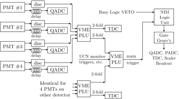
Figure 5: Simplified schematic diagram of the data acquisition event trigger logic.

The frontend electronics for the experiment consisted of a VME-based system for the event trigger logic (via discriminators and programmable logic units (PLUs)) and for the readout of scalers, analog-to-digital convertors (ADCs) and time-to-digital convertors (TDCs). A NIM-based system coupled to the VME system was employed for the implementation of a “busy logic”, which served to veto event triggers arriving during ADC/TDC conversion times (i.e., during these modules’ busy states). This busy logic also prevented re-triggering by correlated scintillator afterpulses (mostly occuring over a $\sim 1$ $\mu$s window junhua_thesis ), and was implemented with a LeCroy 222 gate generator in latch mode.

A simplified schematic diagram of the trigger logic is shown in Fig. 5. For each detector package, a trigger was defined by a two-fold PMT coincidence trigger above the discriminator threshold for each PMT (nominally, set at 0.5 photoelectrons). The resulting two-fold PMT trigger rate in each scintillator was $\sim 50$ s^-1 (primarily from low-energy background gamma rays); the singles rates in each PMT as determined by counting in scalers were typically $\sim 500$–1000 s^-1 (from both dark noise and low-energy backgrounds). The main event trigger was then defined to be the OR of the two detectors’ two-fold PMT triggers and other experiment triggers (e.g., from the ³He UCN monitor detectors). The logic for the two-fold PMT coincidence triggers and the main event trigger was performed with CAEN V495 Dual PLUs. Those main event triggers not vetoed by the busy logic then triggered gate/delay generators for the readout of the ADCs, TDCs, and scaler modules. The total number of two-fold PMT coincidence triggers were counted in scalers as a monitor of the DAQ dead time.

CAEN V775 TDC modules were used for the relative measurement of the time-of-flight between the two detectors’ two-fold PMT coincidence triggers. This relative timing information provided for the identification of the detector with the earlier arriving trigger, important, as discussed later, for the assignment of the initial direction of incidence for electron backscattering events triggering both scintillators. These TDCs were also used to record the timing information from the plastic-scintillator-based muon veto detectors. A global event-by-event time stamp was defined by the counting of a 1 MHz clock in a CAEN V830 scaler.

CAEN V792 charge-integrating ADC (QADC) modules, triggered for readout by a $\sim 140$ ns gate from a CAEN V486 gate/delay generator, provided a measurement of the total charge measured in each PMT. The analog signals from the cosmic-ray muon backing vetos were also read out by these QADC modules. Peak-sensing CAEN V785 ADC (PADC) modules, triggered for readout by a $\sim 12$ $\mu$s gate from a CAEN V462 gate generator, digitized the MWPC anode and cathode-plane signals. Note that the anode signal that was read out was the summation (i.e., single channel per anode plane) of the signals on all 64 of the wires comprising the anode plane. The 64 wires on each of the two cathode planes were read-out in groups of four (i.e., 16 channels per cathode plane); hereafter, we will simply call each of these four-wire groups a “wire”. Analog signals from the ³He UCN monitors and the drift tube cosmic-ray muon veto counters were also read out with PADCs.

The data acquisition (DAQ) system was based on the MIDAS package midas , with a dedicated Linux-based workstation for implementation of the frontend electronics acquisition code and a separate dedicated Linux-based workstation for run control and online analysis. The frontend acquisition code accessed the VME crate via a Struck PCI/VME interface. The MIDAS raw data banks were subsequently decoded into CERNLIB PAW cernlib and ROOT root file formats for data analysis.

A separate data acquisition system, based on the PCDAQ software package hogan99 was used to monitor the proton beam charge incident upon the UCN source’s tungsten spallation target and to asynchronously monitor environmental variables in the experimental area. The incident proton flux was measured using an integrating current toroid mounted around the proton beam line 8 m upstream of the tungsten target, just before the proton beam entered the biological shield. As noted earlier in Section III.2, each proton beam pulse consisted of five 625 $\mu$s beam bursts separated by 0.05 s, with 5.2 s between each pulse’s leading edge burst. The proton charge integrating system measured only the charge of the first of the five beam bursts in each pulse; the resulting value was then scaled by five to yield the total proton charge delivered during each of the 0.2 Hz beam pulses.

The environmental monitoring system asynchronously read and stored up to 96 variables, on a typical time scale of 0.2 s to 1.0 s between readings. Variables measured included cryogenic temperatures in the UCN source (read by Lakeshore 218 temperature monitors), pressures in the different segments of the UCN guide system (read by capacitance manometer, thermocouple, and cold-cathode ion vacuum gauges), ambient temperature in the experimental area, and liquid helium levels and gas pressures throughout the cryogenic systems. The environmental data were time-stamped for later comparison to the $\beta$-decay data acquired with the main data acquisition system.

IV Measurements, Experimental Geometries, and Polarization

In this section we provide a detailed description of our measurement procedures for $\beta$-decay and ambient background runs; the various geometrical configurations of the experiment during our $\beta$-decay runs; and our procedures for, and results from, measurements of the neutron polarization.

IV.1 $\bm{\beta}$-Decay Run Cycle

IV.1.1 Octet Data-Taking Structure

The data taking during normal $\beta$-decay production running was organized into octets, each consisting of A- and B-type quartet run sequences. The structure of these quartet and octet run sequences, shown in Table 2, was such that the neutron spin state (hereafter designated $+$ or $-$, with $+$($-$) corresponding to the loading of UCN with AFP-spin-flipper-on (-off) spin states into the electron spectrometer) was toggled according to a $-++-+--+$ spin-sequence (for octets in which A-type runs preceded B-type runs) or a $+--+-++-$ (i.e., complement) spin-sequence, with the order of $\beta$-decay and ambient background run pairs toggled for a particular spin state within each A-type or B-type run sequence. Within each octet, the decision for whether the A-type runs would precede or follow the B-type runs was made randomly. The notation in Table 2 is such that B^+(-) and $\beta^{+(-)}$ denote, respectively, ambient background and $\beta$-decay runs for the two spin states. The notation for depolarization runs is such that D⁺, for example, denotes a measurement of the depolarized spin-state population for which the spin-state was polarized in the $+$ spin-state during the preceding $\beta$-decay run.

Table 2: Run structure for the octet data taking sequence, consisting of A- and B-type quartets. See text for details.

A1	A2	A3	A4	A5	A6		A7	A8	A9	A10	A11	A12
B-	$\beta^{-}$	D-	B+	$\beta^{+}$	D+		$\beta^{+}$	D+	B+	$\beta^{-}$	D-	B-
B1	B2	B3	B4	B5	B6		B7	B8	B9	B10	B11	B12
B+	$\beta^{+}$	D+	B-	$\beta^{-}$	D-		$\beta^{-}$	D-	B-	$\beta^{+}$	D+	B+

As described in detail later, the $\beta$-decay yields were ultimately obtained from background subtraction. Although such a procedure is potentially subject to systematic bias from time-varying backgrounds, the merit of this octet data-taking structure is that linear background drifts cancel to all orders (provided that the durations of the background and $\beta$-decay runs do not change during the octet) in the definition of asymmetries based on complete octet-structure data sets. Linear drifts in detector efficiency which might affect background subtraction also cancel under the octet structure.

IV.1.2 Run Cycle Procedure

Table 3: Foil thicknesses for the different decay trap end-cap window and MWPC window Geometries and the number of $\beta$-decay events collected in each Geometry passing all analysis cuts.

	Decay Trap End-Cap	MWPC Window	Number of
Geometry (Year)	Window Thickness [$\mu$m]	Thickness [$\mu$m]	$\beta$-Decay Events
A (2008)	0.7 (mylar) + 0.3 (Be)	25	$5.2\times 10^{6}$
B (2008)	13.2 (mylar) + 0.3 (Be)	25	$5.3\times 10^{6}$
C (2008)	0.7 (mylar) + 0.3 (Be)	6	$2.4\times 10^{6}$
D (2009)	0.7 (mylar) + 0.3 (Be)	6	$1.8\times 10^{6}$

As noted previously in Section III.2 and shown in Fig. 2, a gate valve separated the UCN source from the $\beta$-asymmetry experiment. Measurements of the ambient backgrounds (runs A1/B1, A4/B4, A9/B9, and A12/B12) were performed with this gate valve closed (i.e., with no UCN in the decay trap), but with the proton beam still operating in its normal pulsed mode and the AFP spin-flipper in its appropriate run-paired state (i.e., so as to properly account for beam-related backgrounds and any noise/backgrounds associated with the operation of the AFP spin-flipper). These background runs were nominally 0.2 hours in duration. The $\beta$-decay runs (runs A2/B2, A5/B5, A7/B7, A10/B10) were performed with the gate valve open and the AFP spin-flipper in its appropriate state for the entire duration of the run, nominally 1.0 hour in duration.

During the $\beta$-decay runs, an equilibrium density of both correctly polarized and incorrectly polarized UCN developed in the decay trap. With the spin flipper off, the incorrectly polarized population was dominated by depolarization due to material interactions between the UCN and the walls of the decay trap and guides. When the spin flipper was active, this incorrectly polarized population was increased as a result of spin flipper inefficiency. In the spin flipper off case, the lifetime of correctly polarized UCN in the decay trap, dominated by the decay trap exit aperture, was $\sim 21$ s, and the lifetime of incorrectly polarized UCN trapped in the experimental geometry by the 7 T polarizing field was $\sim 31$ s, dominated by losses in the low-field region between the AFP magnet and SCS. In the spin flipper on state, the lifetime of correctly polarized UCN was $\sim 17$ s, and the lifetime of incorrectly polarized UCN was $\sim 44$ s.

At the immediate conclusion of a $\beta$-decay run, a depolarization run (runs A3/B3, A6/B6, A8/B8, A11/B11) was conducted to measure the depolarized fraction of the UCN population in the decay trap via the following procedure. First, the gate valve was closed, the proton beam was gated off, and the switcher valve was re-configured such that the guides downstream of this valve (i.e., from the switcher valve all the way through the decay trap) were connected to a ³He UCN detector (see the discussion in Section III.2). The state of the AFP spin-flipper was unchanged from its state during the immediately preceding $\beta$-decay run. At this point, UCN of the “correct” spin state in the experimental volume could exit the geometry through the 7-T polarizing field, which now served as a spin-state analyzer, and were counted in the UCN detector located at the switcher valve. This cleaning phase lasted 25 s, and the number of counts recorded in the UCN detector during this time interval was proportional to the number of correctly polarized UCN present in the experimental geometry

Following this cleaning phase, the state of the spin-flipper was changed. This then permitted those UCN of the “wrong” spin state located downstream of the spin-flipper, which until now had been trapped within this volume by the 7-T polarizing field, to exit this volume through the 7-T field, and to be counted in the UCN detector. This counting during the unloading phase was performed for $\sim 200$ s, which provided for a measurement of both the number of wrong spin-state neutrons as well as a measurement of the UCN detector background on a depolarization run-by-run basis.

IV.2 Experiment Geometries

During the data-taking runs in 2008–2009 for the results reported in this article, the experiment was operated in four different geometries with different decay trap end-cap and MWPC entrance and exit window foil thicknesses, to study key systematic corrections and uncertainties related to energy loss in, and backscattering from, these foils. The foil thicknesses for these four different experimental geometries, termed Geometries A, B, C, and D, are given in Table 3. The number of $\beta$-decay events collected in each Geometry passing all of the analysis cuts detailed later in this article are also listed there.

Note that although the foil thicknesses for Geometries C and D were identical, we defined separate geometries for these data-taking periods because the UCN transport guides in the region between the APF spin-flip region and the decay trap (i.e., the circular and rectangular guides, see Section III.2) were upgraded from (bare) electropolished Cu in Geometry C to DLC-coated electropolished Cu in Geometry D. This change to a guide system with a higher effective UCN potential in the region downstream of the AFP spin-flip region resulted in a different velocity spectrum for those UCN stored in the decay trap, the details of which were important for the interpretation of measurements of the UCN polarization, described below.

IV.3 Polarization Measurements

A pair of depolarization measurements for each spin state, i.e. a D^- run (following the loading of spin-flipper-off spin states during the preceding $\beta$-decay run) and a D⁺ run (following the loading of spin-flipper-on states) as described in Section IV.1.2, provide, in principle, an in situ measurement of the UCN polarization at the end of the associated $\beta$-decay interval. This pair of measurements automatically incorporates all depolarization mechanisms including, in the case of flipper-on loading, spin flipper inefficiency. Fig. 6 depicts the arrival time spectra in the switcher UCN monitor detector and the decay trap UCN monitor detector (hereafter, SCS monitor detector) characteristic of a depolarization measurement during each of the “load”, “clean”, and “unload” intervals. The states of the gate valve, switcher, and the spin flipper during each of these intervals are indicated schematically there.

Determination of the equilibrium polarization at the end of the “load” interval (corresponding to a time $t=200$ s in Fig. 6) was accomplished by using the switcher UCN detector to count both the number of correctly polarized UCN in the decay trap, $\mathscr{D}_{p}(t=200~{}\text{s})$, during the ”clean” interval, and then by changing the state of the spin flipper to count the number of incorrectly polarized UCN in the decay trap, $\mathscr{D}_{d}(t=225~{}\text{s})$, during the “unload” interval. From these signals, it is possible to extrapolate back to a depolarized fraction $\xi\approx\frac{\mathscr{D}_{d}(t=200~{}\text{s})}{\mathscr{D}_{p}(t=200~{}\text{s})}$ from which detection efficiencies cancel to first order, and which provides the equilibrium polarization via $P=1-2\xi$. The extrapolation procedure requires knowledge of the appropriate storage lifetimes for correctly and incorrectly polarized neutrons in the system, obtained from the SCS monitor detector.

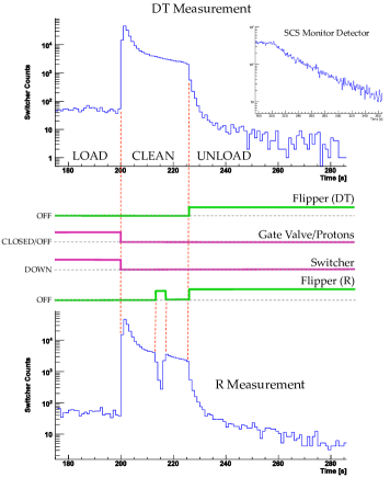
Figure 6: (Color online) Arrival time spectra from the switcher UCN monitor detector (two primary figures) and the SCS monitor detector (top inset figure) characteristic of depolarization trapping (DT) and reloaded background (R) measurements. (The start time $t=0$ corresponds to the start of the load interval or, conceptually, 200 s prior to the end of a $\beta$-decay run.) The states of the gate valve, switcher, and the spin flipper during the load, clean, and unload intervals are indicated schematically. (With the switcher in the “down” state, UCN located between the switcher and the decay trap are transported to the switcher UCN monitor detector; in the opposite state, UCN are transported from the SD₂ source to the electron spectrometer.) The timing and states depicted here are for the case of spin-flipper-off loading. Flipper-on loading measurements reverse the state of the spin flipper.

Models of the UCN transport confirm the intuitive expectation that the time dependence of the “clean” and “unload” switcher detector signals is characterized by double exponential behavior: the shorter time constant is associated with emptying the guide system between the switcher detector and the narrow rectangular guide to the decay trap, while the longer time constant is associated with emptying the decay trap through this rectangular guide. Analysis of the arrival time spectra generated by the $D\pm$ measurements which formed part of the beta asymmetry run cycle was accomplished by first fitting the switcher detector timing spectrum during the clean interval to a double exponential plus background (where the background was determined from the last 100 s of the unload interval). This established the two amplitudes and associated time constants $A^{(+/-)}_{1},\tau^{(+/-)}_{1}$ and $A^{(+/-)}_{2},\tau^{(+/-)}_{2}$ which characterize the population of correctly polarized UCN in the system at the end of the $\beta$-decay (loading) interval, where $-$ corresponds to flipper-off loading and $+$ corresponds to flipper-on loading. Similarly, fitting the unload interval determined the amplitude $A^{(+/-)}_{<}$ associated with the smaller time constant $\tau^{(+/-)}_{<}$ and the amplitude $A^{(+/-)}_{>}$ associated with the larger time constant $\tau^{(+/-)}_{>}$, which ideally characterize the population of incorrectly polarized UCN present at the end of the cleaning interval. In order to extrapolate this population back to the end of the $\beta$-decay measurement interval, the storage lifetimes $\tau_{+/-}$ of UCN trapped in the system due to their spin state relative the state of the spin flipper must also be determined, where here $+$ ($-$) corresponds to the storage lifetime of UCN whose spins are parallel (anti-parallel) to the local magnetic field and are thus trapped downstream of the spin flipper when it is off (on). This was accomplished by fitting the unload interval of the SCS monitor timing spectrum with a single exponential plus background. Note that $\tau_{+}$ is determined during a flipper-on loading (D⁺) depolarization measurement while $\tau_{-}$ is determined during a flipper-off loading depolarization (D^-) measurement. Monte Carlo studies indicated that using these storage lifetimes to capture the average behavior of the depolarized population during the clean interval introduced no significant bias (at the current level of precision) to the extrapolation of this depolarized population back to the $\beta$-decay measurement.

In an ideal depolarization measurement, the cleaning interval is made of sufficient length that contributions to the signal observed during the unloading interval from correctly polarized UCN which are not trapped when the spin flipper changes state are negligible. If the number of free correctly polarized UCN is large and the depolarized signal sufficiently small, however, waiting long enough for adequate cleaning can reduce the incorrectly depolarized signal to levels below the measurement threshold. Since this was the case for the UCNA geometries utilized in the 2008–2009 run period, the cleaning time $\Delta$ was set to 25 s, just long enough to resolve $\tau_{1}$ and $\tau_{2}$. This enhanced the depolarized signal but necessitated separate measurements to determine the correctly polarized background in the unload timing spectrum, which for this clean interval was on the same order as the depolarized signal. In particular, depolarized UCN coming from the decay volume are expected to appear as part of the $A_{<}$ component, but the short cleaning time created a non-negligible population of correctly polarized UCN in the guides between the spin flipper and the polarizing field which are not trapped by the spin flipper and which enter the decay trap before being detected in the switcher detector, causing them to appear as part of $A_{<}$.

In order to correct for this reloaded (R) background, ex situ measurements, denoted $R^{(+/-)}$, were performed. In these measurements, whose characteristic switcher detector timing spectrum is shown in Fig. 6, thirteen seconds prior to the start of the unloading phase the spin flipper state was changed for three seconds in order to trap an additional reloaded population, which then contributed to the amplitude $\widetilde{A}^{(+/-)}_{>}$ determined from the unload phase of the corresponding reload measurement. With this additional observable, the reload-corrected polarizations were determined via

$$P^{-} = 1-2\frac{e^{\Delta/\tau_{+}}\,(\tau^{-}_{>}-\tau^{-}_{<})\,\left\{\zeta^{-}_{1}\,(1-\mathfrak{r}^{-})\,\left[A_{<}^{-}-\mathscr{N}_{-}\widetilde{A}_{<}^{-}\right]+A_{<}^{-}\right\}}{\zeta^{-}_{2}\mathscr{D}_{\mathrm{p}}}~{}~{}~{}~{}~{}\text{(flipper-off loading)}$$

$$P^{+} = 1-2\frac{e^{\Delta/\tau_{-}}\,(\tau^{+}_{>}-\tau^{+}_{<})\,\left\{\zeta^{+}_{1}\,(1-\mathfrak{r}^{+})\,\left[A_{<}^{+}-\mathscr{N}_{+}\widetilde{A}_{<}^{+}\right]+A_{<}^{+}\right\}}{\zeta^{+}_{2}\mathscr{D}_{\mathrm{p}}}~{}~{}~{}~{}~{}\text{(flipper-on loading),}$$

where $\mathfrak{r}$ is a Monte Carlo calculated parameter on the order of 0.60 needed to account for the presence of an extra population between the spin flipper and the 7.0-T region trapped by the three second flipper cycle,

$$\zeta_{1}^{(+/-)}=e^{-(\Delta_{1}+\Delta_{2})/\tau_{2}^{(+/-)}}\;e^{\Delta_{2}/\tau_{(-/+)}}$$ (12)

(where $\Delta_{1}$ is the length of the flipper cycle and $\Delta_{2}$ is the interval between the end of the flipper cycle and the start of the unload phase) is a scaling factor which accounts for the evolution of the reloaded population trapped during the flipper cycle and corrects for the larger population of correctly polarized UCN present to be reloaded during the flipper cycle, $\mathscr{D}_{\mathrm{p}}$ is the total number of background-subtracted counts recorded during the clean interval, $\zeta_{2}$ is a factor which uses $A_{1}$, $\tau_{1}$, $A_{2}$, and $\tau_{2}$ to extrapolate $\mathscr{D}_{\mathrm{p}}$ to the number of counts which would be observed for an infinitely long cleaning period, and $\mathscr{N}$ is a normalization factor. Values of $P^{+}$ and $P^{-}$ were obtained separately for the 2008 and 2009 data sets by summing all corresponding D and R runs and applying Eq. (IV.3). Since there was no statistically significant difference at the 1$\sigma$ level between any of the four measurements, a single reload-corrected value $P$ for the polarization was obtained by performing a weighted average over the four measurements.

Spin flipper inefficiency decreases the UCN polarization for flipper-on loading, resulting in the expectation that $P^{-}>P^{+}$. The resulting decreased polarization for the case of flipper-on loading due to the spin flipper inefficiency is the actual polarization of the UCN population stored in the decay trap, and no further correction to the $P^{+}$ value is required. However, the spin flipper inefficiency also leads to a (smaller) increase in $P^{-}$ since correctly polarized UCN which should remain trapped during the unloading phase are freed when they are not flipped, adding to the observed unload signal. Since this population is generated after the $\beta$-decay measurement interval it requires a correction, which will decrease the value of $P^{-}$. The accumulated data limited this correction to be no larger than $\sim$0.15% of the total polarization, and error bars on $P$ were expanded accordingly. It is also possible to have depolarized UCN populations whose storage lifetime in the system is much shorter than the depolarization measurement time, and which therefore have a low efficiency for detection in a depolarization measurement. Neutrons with sufficient energy to surmount the potential barrier presented by the 7.0-T polarizing field (which may therefore enter the experiment in the wrong spin state) and initially polarized UCN with energies higher than the material potential of the decay trap walls (which can survive in the system when confined to trajectories that sample the walls at sufficiently oblique angles) are examples of such populations. Monte Carlo calculations estimating the effect of these populations on the neutron polarization indicated a negligible contribution at the current level of precision, due largely to the short residency times that such UCN posses. Expanding the error bars on $P$ to account also for variations in the polarization due to pulsed loading (estimated to be on the order of 0.04% of $P$), a 1$\sigma$ lower limit of $P>0.9948$ was determined.

V Calibration and Reconstruction

We now turn to a discussion of our data analysis and energy calibration procedures. We begin by defining the various possible event types in the experiment, the selection rules for the observable event types, and a desciption of our position recontruction algorithm using the MWPC signals. We also discuss our data “blinding” procedure, which ultimately resulted in “blinded” asymmetries which were scaled by a randomly chosen scaling factor at the $\mathcal{O}$(0–5%) level. Next, we discuss our energy calibration procedures for the scintillator and the MWPC, and then compare for the different event types our reconstructed energy spectra with simulated Monte Carlo spectra. Finally, we conclude this section with a discussion of our procedure for the assignment of the initial energy of the electron.

Hereafter, in our discussions of the data analysis of the detector signals, we will refer to the two electron detectors as the “East” and the “West” detectors, corresponding to their actual physical locations in the UCNA Experiment.

V.1 Event Type Definitions

Figure 7: Schematic diagram of the various event types defined in the text.

Measurement of the $\beta$-asymmetry requires an accurate determination of the decay electron’s initial direction of incidence. This determination is complicated by backscattering effects, some of which are not detectable. We define the various classes of event types, shown in Fig. 7.

• No backscattering events: Events in which an electron, incident initially on one of the detectors, does not backscatter from any element of that detector, and then generates a two-fold PMT trigger in that side’s scintillator.

• Type 1 backscattering events: Events in which an electron, incident initially on one of the detectors, generates a two-fold PMT trigger in that side’s scintillator, backscatters from that scintillator, and then generates a two-fold PMT trigger in the opposite side’s scintillator. Note that a measurement of the relative time-of-flight between the two scintillators’ two-fold PMT triggers determines the initial direction of incidence for Type 1 backscattering events.

• Type 2 backscattering events: Events in which an electron, incident initially on one of the detectors, deposits energy above threshold in that side’s MWPC, backscatters from some element of that side’s MWPC (e.g., gas, wire planes, or the exit window) or the scintillator without generating a two-fold PMT trigger (e.g., backscattering from the scintillator’s dead layer, or triggering only one PMT), and is then detected in the opposite side’s scintillator. As can be seen in Fig. 7, the initial direction of incidence of a Type 2 backscattering event would be misidentified using only scintillator two-fold PMT trigger information.

• Type 3 backscattering events: Events in which an electron, incident initially on one of the detectors, generates a two-fold PMT trigger in that side’s scintillator, backscatters from that side’s scintillator, deposits energy above threshold in the opposite side’s MWPC, and is then stopped in some element of the opposite side’s MWPC or scintillator without generating a two-fold PMT trigger (i.e., in the dead layer, or triggering only one PMT). Note that Type 2 and Type 3 backscattering events cannot be distinguished using only scintillator two-fold PMT trigger information and a threshold cut on the MWPC response (i.e., the Type 2 and Type 3 events depicted in Fig. 7 would not be distinguishable).

• Missed backscattering events: Events in which an electron, incident initially on one of the detectors, backscatters from either the decay trap end-cap foil or that side’s MWPC without depositing energy above threshold (e.g., from the entrance window, or from the gas in the region between the cathode plane and the entrance window), and is then detected in the opposite side’s MWPC and scintillator. Note that missed backscattering events cannot be identified experimentally.

• Lost events: Events in which an electron, incident initially on one of the detectors, deposits significant energy in a decay trap end-cap foil and/or the MWPC, and does not generate a two-fold PMT trigger in either of the scintillators. Note that because these events do not generate a DAQ event trigger, they cannot be identified experimentally.

No backscattering events and Missed backscattering events cannot be distinguished experimentally, and are, hereafter, termed “Type 0” events. Based on scintillator information alone, Type 2 backscattering events cannot be distinguished from Type 3 backscattering events. Thus, we will refer to these types of events as “Type 2/3” events. Later in Section VI.1.2 we will discuss the separation of Type 2/3 events using MWPC information and simulation input. Finally, Lost events cannot, of course, be reconstructed and can only be corrected for in simulation.

V.2 Run Selection

Proton beam delivery constraints and other experimental issues prevented on occasion the accumulation of complete octet data sets during normal $\beta$-decay production running. In the absence of a complete octet, runs forming a quartet (i.e., runs A1–A12 or B1–B12 in Table 2) or spin-pair (i.e., A1–A6, A7–A12, B1–B6, or B7–B12) were retained for analysis. Runs with clear detector issues (e.g., noisy channels associated with the MWPC cathode planes) were discarded.

V.3 Data Blinding

We performed a blinded analysis of our asymmetry data by applying separate spin-dependent randomly chosen scaling factors to the two detectors’ count rates, thus effectively adding an unknown scaling factor to the measured asymmetry. This was implemented via the following procedure. First, note that the detector count rates were based on a global event-by-event clock time which was defined, as described earlier in Section III.8, by counting a 1 MHz clock in a scaler. Second, we generated two random scale factors, $f_{1}$ and $f_{2}$, which were constrained to be between $1.00\pm(0.05\times 0.04)$, where 0.04 represents the approximate value of the measured asymmetry.

For runs with the AFP spin-flipper on ($+$ spin state), we then scaled the east and west detector clock times, $t_{E}^{+}$ and $t_{W}^{+}$, by these scale factors according to

$$t_{E}^{+}=t\cdot f_{1},~{}~{}~{}~{}~{}~{}~{}~{}~{}~{}t_{W}^{+}=t\cdot f_{2},$$ (13)

where $t$ denotes the true global clock time. Similarly, for those runs with the AFP spin-flipper off ($-$ spin state),

$$t_{E}^{-}=t\cdot f_{2},~{}~{}~{}~{}~{}~{}~{}~{}~{}~{}t_{W}^{-}=t\cdot f_{1}.$$ (14)

In calculating the super-ratio for a spin-state run pair according to Eq. (10), the resulting blinded measured asymmetry, $A_{\text{blind}}$, is then a function of the blinded and true super-ratios, $R_{\text{blind}}$ and $R_{\text{true}}$, according to

$$A_{\text{blind}}=\frac{1-\sqrt{R_{\text{blind}}}}{1+\sqrt{R_{\text{blind}}}}=\frac{1-f\sqrt{R_{\text{true}}}}{1+f\sqrt{R_{\text{true}}}},$$ (15)

where $f\equiv f_{2}/f_{1}$.

All of our analysis was performed with these blinded asymmetries. Note that this did not impact our assessment of our energy reconstruction algorithms (which do not, of course, depend on the asymmetry), or our assessment of our systematic corrections for backscattering and the $\cos\theta$-dependence of the acceptance, as these were calculated (and subsequently benchmarked) in units of $A_{0}$.

V.4 Data Quality Cuts and Live Time Definition

We subjected each run to a number of so-called “global” and “event-by-event” data quality cuts, resulting in the removal of either a consecutive range of events or a single event, respectively. First, we note that there were sporadic corruptions to the data stream resulting from malfunctioning DAQ electronics modules. These electronics problems resulted in either the corruption of all subsequent events following the occurence of the problem, or the corruption of only a single isolated event. Electronics problems resulting in the corruption of all subsequent events included misalignments of the VME data banks (e.g., of the QADC data bank relative to the PADC data bank) and sudden shifts in the TDC channel peak positions of the two detectors’ two-fold PMT self-trigger timing peaks. After the identification of either of these problems, a global data quality cut was applied, resulting in the removal of all subsequent events in that run. Electronics problems which resulted in the corruption of only a single event included corruptions to the headers and/or footers of the PADC, QADC, or TDC event banks (e.g., an event lacking a header or footer) and corruptions to the TDC bank event counter relative to the MIDAS data acquisition event counter. An event-by-event data quality cut was then applied to those events found to have either of these latter two types of electronics problems.

A significant fraction of the data acquired during the Geometries A and B running was discarded due to the above-described electronics problems. In particular, of the data acquired during the second half of the Geometry A running and then during the entire Geometry B running, $\sim 5$% of the events lacked a header and/or footer and up to $\sim 30$% of the events suffered from the TDC bank event counter problem. In contrast, the fraction of events suffering from electronics problems acquired during the Geometries C and D running was small, with $<5$% of the data affected by these problems.

Other global data quality cuts included the removal of all events between 0.00 s to 0.05 s after each proton beam burst. Typical scintillator two-fold PMT trigger rates during the 0.2 Hz proton beam beam pulse repetition cycle are shown in Fig. 8. As can be seen there, the peak scintillator trigger rates were up to a factor of $\sim 80$ higher during the proton beam bursts. This figure illustrates one of the merits of a pulsed-spallation-source of UCN, namely, that the experiment can be performed in a low background environment (i.e., ambient backgrounds only) during the time between the proton beam bursts. Another global data quality cut included the removal of events from $\beta$-decay runs occuring during time periods when the rate on the ³He UCN monitor detector located near the gate valve dropped below some threshold were vetoed, so as not to degrade the signal-to-background ratio.

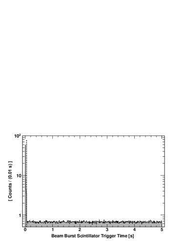
Figure 8: Typical scintillator two-fold PMT trigger rates during the 0.2 Hz proton pulse repetition cycle. For the clock timing shown here, each of the five beam bursts comprising each proton pulse occur at $t=0$, as the clock was reset to $t=0$ with each beam burst; thus, under this reset scheme, all of the events collected during the five beam bursts appear between 0 and 0.05 s (as noted in Section III.2, the time between beam bursts was 0.05 s). The dashed line indicates the cut at 0.05 s.

After application of the above-described global data quality cuts, we then computed on a run-by-run basis a “live time” for each detector, defined to be the sum of the (blinded) clock times of the run segments surviving the above-described global data-quality cuts. Specifically, if a run segment between event $M$ and event $N>M$ survived these global data-quality cuts, the corresponding east and west detector live times, $T_{E}$ and $T_{W}$, for this run segment were calculated as

$$T_{E}=t_{E}^{N}-t_{E}^{M},~{}~{}~{}~{}~{}~{}~{}~{}~{}~{}T_{W}=t_{W}^{N}-t_{W}^{M},$$ (16)

where $t_{E}^{M}$ ($t_{W}^{M}$) and $t_{E}^{N}$ ($t_{W}^{N}$) denote the blinded time stamps for the east (west) two-fold PMT trigger for events $M$ and $N$, respectively, defined previously in Eqs. (13) and (14).

We note, however, an exception to the above-described procedure under which we applied an event-by-event data quality cut to events with a TDC event counter problem (with no subsequent correction to the live time). In particular, as was already noted, up to $\sim 30$% of the events collected during the Geometry B running suffered from this problem. Further, the fraction of corrupted events recorded by each detector differed for the two neutron spin states, thus biasing the extracted asymmetry. Thus, it was necessary to correct the Geometry B live times. As discussed later in Section VIII.6, we corrected for this Geometry B live time problem using background gamma-ray events, which were uncorrelated with the neutron $\beta$-decay events. The correction factors to the live times were then defined for each detector on a run-by-run basis to be the ratio of the number of gamma-ray events surviving the event-by-event TDC event counter cut to the total number of recorded gamma-ray events.

V.5 Event Reconstruction and Identification

Those events surviving the above data-quality checks were then reconstructed and identified (i.e., tagged as a Type 0, Type 1, or Type 2/3 event) based on the TDC measurement of the two detectors’ two-fold PMT coincidence trigger time-of-flight, the pulse height (PADC) in the MWPCs, and the pulse height (PADC and QADC) and timing (TDC) information from the various muon-veto detectors. The available detector information is described in more detail below.

Figure 9: Typical two-fold coincidence trigger relative time-of-flight spectrum for one of the scintillator detectors from a $\beta$-decay run. See text for details.

V.5.1 Scintillator Timing Information

The logic outputs from the PLUs defining the two-fold PMT triggers for the two detectors were routed to TDC channels, forming the STARTs for their respective channels. A copy of the main event trigger was delayed by $\sim 155$ ns and was used to generate the COMMON STOP for the TDC. A typical two-fold coincidence trigger time-of-flight spectrum for one of the detectors (for example, of the West detector) is shown in Fig. 9. Main event triggers generated by a West detector two-fold trigger appear at the self-trigger delay time of $\sim 155$ ns, whereas main event triggers generated by a East detector two-fold trigger, with no later arrival of a West detector two-fold trigger, appear at the peak at 0 ns (i.e., a “time-out” for that TDC channel). Those events forming the broad secondary peak from $\sim$ 20–140 ns, separated from the self-trigger peak by the dashed line, correspond to main event triggers generated by a East detector two-fold trigger, with the later arrival of a West detector two-fold trigger. That is, Type 1 backscattering events incident initially on the (opposite-side) East detector comprise this broad peak. The backscattering cut line (the dashed line in Fig. 9 at 140 ns) placed approximately 15 ns before the self-timing peak is justified by the fact that the minimum time-of-flight (i.e., straight-line trajectory) for an 800 keV electron ($\beta$ = 0.919) traveling the 4.4 m distance between the two scintillators is 15.9 ns.

Note that for the TDC dynamic range setting of $\sim 140$ ns shown in Fig. 9, a “true” Type 1 event with a coincidence time-of-flight greater than $\sim 140$ ns would not appear in the opposite-side detector’s coincidence timing spectrum, but would instead appear in its “time-out” peak; therefore, such a “true” Type 1 event would be misidentified in data analysis as a Type 2/3 event. However, as calculated in simulation, the fraction of Type 1 events with a time-of-flight greater than $\sim 140$ ns is small, $\sim 2$%, and results in a negligible effect on the asymmetry.

V.5.2 MWPC Spectra and Particle Identification

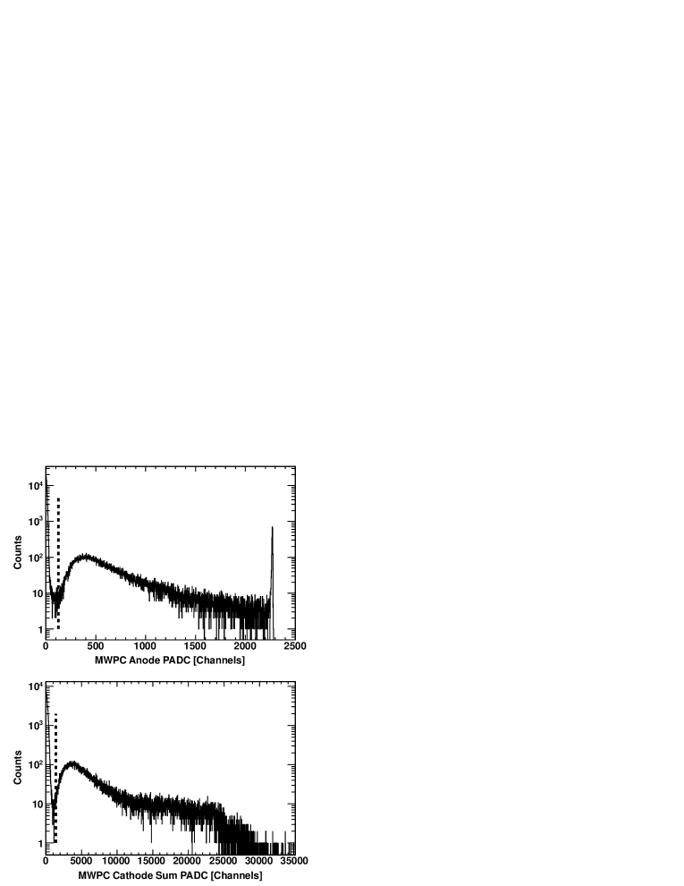
Figure 10: Typical MWPC anode and summed cathode pulse height spectra from a $\beta$-decay run. The dashed lines indicate the cut positions. The peak in the anode spectrum at channel $\sim 2250$ is overflow. Because the cathode sum is obtained via summation over all of the individual cathode channels, channel overflows are distributed throughout the summed spectrum.

As noted earlier, the MWPC anode and cathode pulse height signals were read out on PADC channels during a $\sim 12$ $\mu$s window after each event trigger. Typical anode and cathode (summed over all of the individual cathode channels) pulse height spectra during a $\beta$-decay run are shown in Fig. 10. For scintillator event triggers, the majority of the events appeared in the pedestal, and were tagged as gamma ray events. Those events satisfying a cut on either the anode PADC channel number or the summed cathode PADC channel number, indicated by the dashed lines there, were identified as charged particles (electrons or muons). Electron hits in a particular scintillator were then further separated from muon hits by the requirement of no coincident hits in any of the same-side muon veto detectors. Note that the coincidence window for the plastic scintillator (drift tube) muon veto detectors was defined by the $\sim 140$ ns ($\sim 12$ $\mu$s) QADC (PADC) data acquisition gate.

After removal of the events occuring during the pulsed proton beam bursts, the requirement of a MWPC-scintillator coincidence cut further reduced the total integrated ambient background rate in each scintillator by a factor of $\sim 40$ from $\sim 50$ s^-1 to $\sim 1.2$ s^-1 over the range of QADC channels corresponding to the neutron $\beta$-decay energy spectrum. This is illustrated in Fig. 11, where the (uncalibrated) scintillator spectrum in QADC channels for a typical background run is shown with and without the requirement of a MWPC-scintillator coincidence for a typical background run. The resulting broad peak centered approximately at channel 5000 is from minimum-ionizing cosmic-ray muons. The origin of the surviving low-energy tail (channels $\lesssim 2000$) was demonstrated in Monte Carlo studies to be the result of cosmic-ray muon interactions with spectrometer materials (e.g., in the SCS magnet’s infrastructure) located near the MWPC and scintillator detector, such as $\delta$-ray production and Compton scattering of muon-induced gamma rays.

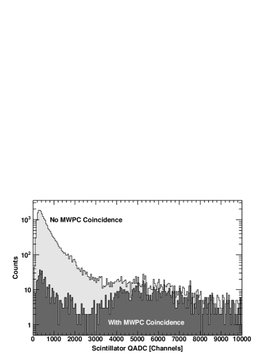
Figure 11: Typical scintillator spectrum for a background run, without (light shaded) and with (dark shaded) the requirement of a MWPC coincidence cut. See the text for a description of the features in the resulting concidence spectrum.

V.5.3 Event Type Classification

Table 4: Detector selection criteria (scintillator two-fold PMT TDC trigger timing and MWPC pulse height) for the identification of Type 0, Type 1, and Type 2/3 events. A $\surd$ indicates the requirement of a valid detector hit, whereas a $\times$ indicates the requirement of no detector hit. The notation (*) indicates the requirement of an earlier detector hit relative to the opposite-side detector hit.

Event Type	East Detector		West Detector
	TDC	MWPC	TDC	MWPC
Type 0 East Incidence	$\surd$	$\surd$	$\times$	$\times$
Type 0 West Incidence	$\times$	$\times$	$\surd$	$\surd$
Type 1 East Incidence	$\surd$ (*)	$\surd$	$\surd$	$\surd$
Type 1 West Incidence	$\surd$	$\surd$	$\surd$ (*)	$\surd$
Type 2/3 East Trigger	$\surd$	$\surd$	$\times$	$\surd$
Type 2/3 West Trigger	$\times$	$\surd$	$\surd$	$\surd$

Electron events were classified as Type 0, Type 1, or Type 2/3 events according to the detector selection criteria listed in Table 4. Electron events not satisfying any of these criteria were discarded.

For Type 0 events, the assignment of the initial direction of incidence (i.e., on the East or West detector) was, of course, trivial. For Type 1 events, the initial direction was determined from the TDC two-fold trigger time-of-flight spectra, as discussed earlier in Section V.5.1. At this stage of the analysis, Type 2/3 events were identified as such but were only tagged with the triggering scintillator side (i.e., not yet assigned an initial direction of incidence).

V.6 MWPC Position Reconstruction

V.6.1 Algorithm

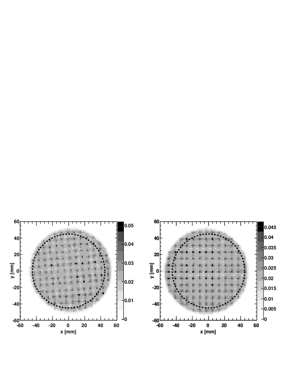
Figure 12: Distributions of $(x,y)$ position distributions [for the coordinate system choice (4) described in the text] for Type 0 neutron $\beta$-decay events (left panel: East detector, right panel: West detector). The dashed circles denote the nominal 45 mm fiducial volume radius cut. The regularly-spaced “spikes” are an artifact of the position reconstruction algorithm: for events in which two adjacent cathode channels recorded overflow values, the algorithm reconstructed the positions to sharp peaks halfway between the two wires’ positions (as discussed in Section V.6.1).

The transverse $(x,y)$ position of an event was reconstructed from the charge distribution on the MWPC cathode plane wires. The position reconstruction algorithm that was employed for the calculation of the position from the signals that were digitized by the PADC modules began by identifying, on each of the $x$- and $y$-planes, the wire with the maximum PADC readout value above pedestal. The position was then reconstructed from the PADC reading of this “maximum wire” and those of the immediately adjacent wires, with all other wires ignored, by fitting these three wires’ PADC readings as a function of their $x$- or $y$-positions to a Gaussian shape. The positions for $\sim 90$% of the neutron $\beta$-decay events could be reconstructed with this algorithm.

The positions for the remaining $\sim 10$% of the events were reconstructed under various special circumstances. For example, if there was only one wire with a PADC value above pedestal, the position was assigned to that particular wire’s coordinate. Or if only one of the wires directly adjacent to the maximum wire recorded a PADC value above pedestal, or if the maximum wire was located on one of the cathode plane edges and the adjacent wire recorded a PADC value above pedestal, the position was determined under the assumption that the width of the charge distribution was 0.75 times the wire spacing (as determined from the $\sim 90$% of the events reconstructed with the three-wire Gaussian fitting algorithm). In the event two or more wires recorded overflow PADC values, the positions were reconstructed to sharp peaks halfway between the two overflow wires’ coordinates.

Finally, if the $x$- or $y$-position could not be reconstructed (e.g., if none of the wires on one or both the cathode planes recorded a PADC value above pedestal), the $x$- or $y$-position was defined to be 0.0. This was potentially the source of a systematic bias, because as is discussed in detail later in Section V.8, the scintillator energy reconstruction was position dependent. However, the fraction of events identified as charged particles failing either the $x$- or $y$-reconstruction was small, $<10^{-3}$, and is consistent with our later estimate (Section VIII.9) of the MWPC efficiency. The origin of these events may have been electronic noise on the MWPC anode channel correlated with a scintillator trigger, thus resulting in the identification of the event as a charged particle with no corresponding signal on the cathode PADC channels.

Note that all of the $(x,y)$ position spectra shown hereafter have been projected back to the spectrometer’s 1.0-T field region from the 0.6-T field-expansion region.

V.6.2 Position Cuts, Fiducial Cut, and Coordinate Systems

The reconstructed positions were used to define a fiducial volume in order to reject events originating near the decay trap collimator (inner radius of 58.4 mm). Examples of such problematic events include both $\beta$-decay electrons (subject to $\cos\theta$-dependent acceptance and backscattering effects) and background electrons from the Compton scattering of gamma rays in the decay trap material.

For Type 0 events, we required the reconstructed radius on the triggering scintillator side to satisfy a conservative $r_{\text{trigger}}<45$ mm cut. The maximum Larmor diameter for an endpoint energy electron in the 1.0-T spectrometer field was 7.76 mm; thus, this 45 mm cut was safely located $\sim 2$ Larmor diameters from the decay trap wall. For events identified as Type 1 or 2/3 backscattering events, in addition to this $r_{\text{trigger}}<45$ mm trigger-side cut, we also made a further cut on the two sides’ $\vec{x}_{E}-\vec{x}_{W}$ vertex difference to eliminate accidental backgrounds, with this cut defined to be $|\vec{x}_{E}-\vec{x}_{W}|<25$ mm.

To study possible systematic effects associated with the position reconstruction, we considered four different coordinate systems. (1) Coordinates defined by their nominal positions reconstructed from the just-described Gaussian fits to the wires’ PADC readings: $\vec{x}_{E}=(x_{E},y_{E})$ and $\vec{x}_{W}=(x_{W},y_{W})$. (2) West-side coordinates defined by their nominal positions, $\vec{x}_{W}$, but transformed East-side coordinates $\vec{x}^{\prime}_{E}=(x^{\prime}_{E},y^{\prime}_{E})$ based on fits to Type 1 backscattering data which provided for a detector-to-detector coordinate system based on these backscattering measurements of the detector-pixel-to-detector-pixel magnetic field map. These fits were of the form $\vec{x}^{\prime}_{E}=\mathcal{R}\vec{x}_{E}+\vec{c}$, where $\mathcal{R}$ denotes a rotation matrix, and $\vec{c}=(c_{x},c_{y})$ is a constant offset vector. (3) Coordinates defined by the complement of (2) (i.e., East-side coordinates defined by their nominal positions, but West-side coordinates transformed according to the Type 1 backscattering detector-pixel-to-detector-pixel magnetic field map). (4) A “split” coordinate system, in which the rotation matrix $\mathcal{R}$ was applied to one set of coordinates, with the constant offset vector $\vec{c}$ split between the two detectors, such that $\vec{x}^{\prime}_{E}=\mathcal{R}\vec{x}_{E}+\vec{c}/2$, and $\vec{x}^{\prime}_{W}=-\vec{c}/2$. The latter was chosen as the default coordinate system in the analysis presented hereafter. We assess the systematic uncertainty associated with our choice of a coordinate system in Section VIII.4.

Sample $(x,y)$ position distributions [calculated for the coordinate system choice (4) described in the above paragraph] extracted from the East and West MWPC for Type 0 neutron $\beta$-decay events (after background subtraction) are shown in Fig. 12. The distribution of background events was previously shown to be uniform over the MWPCs’ sensitive areas plaster08 .

V.7 Monte Carlo Simulation Programs

We developed two independent Monte Carlo simulations of the experimental acceptance, based on the GEANT4 (version 9.2) geant4 and PENELOPE (version 3) penelope simulation codes. These were employed extensively as input to our energy calibration procedures (described next) and for calculations of the systematic corrections for backscattering and the $\cos\theta$-dependence of the acceptance (e.g., from suppression of the acceptance at large angles), discussed in detail in Section VII. The performance of these simulation programs was benchmarked previously in a series of measurements of backscattering from beryllium, plastic scintillator, and silicon targets and found to be accurate to within 30% in their predictions for the angular and energy distributions of the backscattered electrons junhua_thesis ; martin03 ; martin06 ; hoedl_thesis .

Both of these simulations included detailed geometric models for: (1) the 3-m long decay trap and its end-cap foil geometry; (2) the MWPCs, including their entrance and exit windows, the Kevlar fiber support for the entrance windows, the anode and cathode wire planes, and the 100 Torr neopentane fill gas; (3) the two dead regions in the MWPC (i.e., the two regions between the cathode planes and the entrance/exit windows); (4) the plastic scintillator disc; (5) the measured scintillator dead layer of 3.0-$\mu$m thickness junhua_thesis ; and (6) the magnetic field in the decay trap and field expansion regions. Note that depending on the study of interest, the magnetic field was modeled either as a perfectly uniform 1.0-T field in the decay trap region analytically connected (subject to the $\vec{\nabla}\cdot\vec{B}=0$ requirement) to the 0.6-T field in the field-expansion region, or via bicubic spline interpolation of a three-dimensional grid of the field profile (e.g., such as for the measured field profile shown in Fig. 4). In both the GEANT4 and PENELOPE simulations, charged particles were transported through the magnetic field via Runge-Kutta integration of the equations of motion.

For simulation studies of calibration sources, events were generated isotropically into $4\pi$ from a fixed point, with a model for the source foil covers (assumed to be 3.6-$\mu$m mylar). For neutron $\beta$-decay simulations, events were generated uniformly over the decay volume. The GEANT4 events were emitted isotropically into $4\pi$ and then weighted with a $W(\theta)\propto(1+A\beta\cos\theta)$ weight factor, whereas the PENELOPE events were sampled from the full phase-space distribution of Eq. (4).

V.8 Visible Energy Calibration

V.8.1 Overview

The overarching goal of the energy calibration procedure was to calibrate the quantity of scintillation light produced by an electron which deposited a certain amount of “visible energy” in the scintillator and to calibrate the electron energy deposition in the MWPC fill gas. We define the scintillator visible energy, $E_{\text{vis}}$, to be the total energy loss in the scintillator active region (i.e., beyond the dead layer) measured by the photomultiplier tubes. The scintillator visible energy is, of course, not equal to the initial energy of the emitted $\beta$-decay electron, due to reconstructable energy loss in one or more of the MWPCs’ active regions, and non-reconstructable energy loss in one or more of the decay trap end-cap foils, one or more of the MWPCs’ non-active elements (e.g., windows, wire planes, and gas region between the cathode planes and the windows), and in one or more of the scintillators’ dead layers. The relationship between the measured visible energy in the scintillator, the measured energy deposition in the MWPC, and the reconstructed “true” initial energy of the $\beta$-decay electron, denoted $E_{\text{recon}}$, was determined via comparison of conversion electron source measurements to Monte Carlo studies (as discussed in Section V.14).

As described earlier in Section III.5.3, each PMT effectively viewed one $\pi/2$ quadrant of the scintillator; therefore, the response of each PMT was expected to vary as a function of the $(x,y)$ position of the event. Each PMT then produced a signal which was a nonlinear function of the scintillation light it viewed, with the nonlinearity the result of known physics (i.e., quenching interactions in the scintillator birks51 ) and also hardware response issues. The scintillation light was then ultimately digitized by the QADC data acquisition modules. Accounting for a time-dependent gain of the PMT/QADC system, the total response of the system to PMT $i$ in terms of digitized QADC channels was then modeled as

$$\text{QADC}_{i}=g_{i}(t)\cdot f_{i}(\eta_{i}(x,y)\cdot E_{Q}),$$ (17)

where $E_{Q}$ denotes the light produced in the scintillator, $\eta_{i}(x,y)$ is the fraction of that light reaching PMT $i$ from the position $(x,y)$ of the event, $f_{i}$ is the (possibly non-linear) response function of PMT $i$, $g_{i}(t)$ denotes the time-dependent gain fluctuation of PMT $i$, and $\text{QADC}_{i}$ is the digitized readout for the event. Note that we use the notation $E_{Q}$ for the produced scintillation light because the produced light should be proportional to the “quenched energy”, which we define to be the true energy deposition reduced by a Monte-Carlo-calculated quenching factor (based on studies with a low-energy electron gun junhua_thesis ; yuan01 ). The QADC readout signal that is measured also includes statistical fluctuations due to photoelectron (PE) counting statistics, with the number of PEs proportional to the scintillation light transported to the PMT, $N_{i}\propto\eta_{i}(x,y)E_{Q}$, with the fluctuations in $N_{i}$ expected to follow a Poisson distribution.

The scintillator energy calibration procedure was thus divided into three primary tasks: (1) a determination of the linearity function $f_{i}$ for each PMT; (2) a determination of the light-transport efficiency $\eta_{i}(x,y)$ position response map for each PMT; and (3) a determination of the time-dependent gain $g_{i}(t)$ for each PMT. Detailed descriptions of each of these tasks follow below. However, note that the overall calibration procedure was highly iterative, whereby previous approximate results from the other two tasks were used to produce new, more refined results for the task in question. Therefore, our discussions below of the individual tasks reference input from the other two tasks.

V.8.2 PMT Linearity Functions

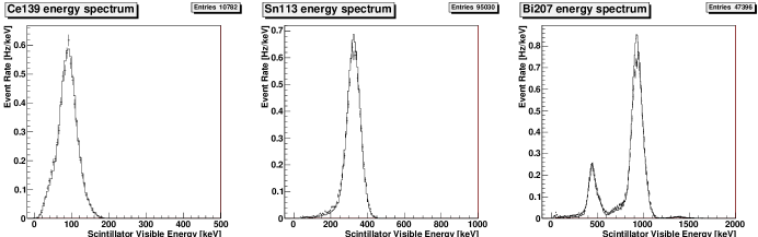
Figure 13: Calibrated $E_{\text{vis}}$ visible energy spectra (data points with error bars), compared with Monte Carlo calculations (solid lines), for three of the calibration sources: ¹³⁹Ce (left panel), ¹¹³Sn (middle panel), and ²⁰⁷Bi (right panel).

The $f_{i}$ response functions for each of the PMTs were determined each time a new set of calibrations was performed at multiple $(x,y)$ positions with the conversion electron sources using the remote source insertion system described previously in Section III.6. Most of the useful calibration data were obtained with the ¹³⁹Ce, ¹¹³Sn, and ²⁰⁷Bi sources; however, note that the ¹³⁹Ce source was not available during data taking for Geometries A and B. The ¹⁰⁹Cd source was visible only in Geometries C and D (configuration with 6-$\mu$m MWPC windows).

The QADC spectra for each PMT were then recorded for each $(x,y)$ source position. The expected $E_{Q}$ spectrum for each PMT for each $(x,y)$ source position was then determined from the Monte Carlo simulation programs, with the Monte Carlo spectrum further smeared by the PE counting statistics. The smeared Monte Carlo spectrum was then fit to a Gaussian (or, two Gaussians for the case of ²⁰⁷Bi) to determine the $E_{Q}$ of the source conversion electron peaks. The measured QADC spectrum was also fit according to the same procedure, thereby providing the measured QADC peak location for each conversion electron peak. Note, however, in order to prevent PMT nonlinearity from shifting the fit position, the QADC spectrum was first linearized using a linearity function $f_{i}$ determined from an earlier iteration of this procedure. The linearized spectrum of $f_{i}^{-1}(\text{QADC}_{i})$ was then fit, and the peak positions were converted back to nonlinear QADC values via the $f_{i}$ functions. Figure 13 shows sample data compared with Monte Carlo spectra of the visible energy $E_{\text{vis}}$ for three of the calibration sources (¹³⁹Ce, ¹¹³Sn, and ²⁰⁷Bi).

Figure 14: Two examples of PMT linearity curves, for a PMT exhibiting a nearly linear response (left panel) and a PMT exhibiting a highly nonlinear response (right panel). The curves are fits to the measured QADC values (horizontal axis) of the peaks for the various calibration sources at different $(x,y)$ positions versus the expected light reaching each PMT. The large nonlinearity observed in some PMTs was traced to damaged bases and subsequently repaired for runs after 2009.

Using the position response map $\eta_{i}(x,y)$ for each PMT, the expected light reaching each PMT $\eta_{i}(x,y)\cdot E_{Q}$ was plotted against the observed QADC values of the peaks for the various sources at the various $(x,y)$ positions. The points on these plots thus trace out the linearity curve for each PMT, with a fit to the $\eta_{i}(x,y)\cdot E_{Q}$ values as a function of the QADC values providing a parametrization of the linearity function $f_{i}^{-1}$ for each PMT. Examples of such linearity curves are shown in Fig. 14 for two of the PMTs, with one of the PMTs exhibiting a nearly linear response, and the other a highly nonlinear response. The linearity curves were parametrized with a fit function which was purely linear below some manually-determined transition point $x_{0}$. Above this $x_{0}$, the nonlinearities were parametrized in the form $y(x)=\exp[C_{1}+\ln x+C_{2}[\ln(x/x_{0})]^{2}+C_{3}[\ln(x/x_{0})]^{3}]$, with $C_{1}$, $C_{2}$, and $C_{3}$ fitted constants.

V.8.3 PMT Position Response Maps

The overall principle for the determination of the light transport efficiency to each PMT as a function of position, $\eta_{i}(x,y)$, was to employ the measured neutron $\beta$-decay spectrum endpoint as a “standard candle” providing coverage over the entire detector fiducial volume. Assuming the linearity and time-dependent gain functions, $f_{i}$ and $g_{i}(t)$, are known, the measured data provide a measure of the amount of light reaching each PMT, $L_{i}(x,y)\equiv\eta_{i}(x,y)\cdot E_{Q}=f_{i}^{-1}(\text{QADC}_{i}/g_{i}(t))$. The spectrum of $L_{i}(x,y)$ has the same shape as the spectrum of $E_{Q}$, but is linearly “stretched” by the light-transport factor $\eta_{i}(x,y)$. Determining the absolute light-transport efficiency would be quite difficult, but, fortunately, is unnecessary. Instead, measuring the relative efficiency between different $(x,y)$ locations is sufficient, normalizing $\eta_{i}$ by convention to $\eta_{i}(0,0)=1$, and leaving the unknown constant factor between the $\eta_{i}$ and the absolute (unknown) light-transport efficiencies to be absorbed into the $f_{i}$.

In principle, the relative $\eta$ between two different locations can be determined by seeing how much the $L_{i}$ spectrum at one point needs to be “stretched” to line up with the spectrum at another point. In practice, the stretching factor $\eta_{i}(x,y)$ was determined so that a Kurie plot of $\eta_{i}(x,y)\cdot L_{i}(x,y)$ was aligned with a Kurie plot of a smeared Monte Carlo visible energy spectrum. To find the necessary $\eta_{i}(x,y)$, an iterative Kurie plotting procedure was used. Starting from an initial guess $\eta_{i,0}(x,y)$ for each $\eta_{i}(x,y)$, a Kurie plot was then made from the spectrum of $\eta_{i,0}(x,y)\cdot L_{i}(x,y)$. This plot was fit with a straight line over a visible energy range from 250–700 keV, which yielded some intercept $E_{\text{int}}$. The position of this fitted intercept relative to the expected intercept (from the Monte Carlo visible energy spectrum smeared by the PE counting statisics), $E_{\text{MC}}$, then provided an improved estimate for the stretching factor, $\eta_{i,0}^{\prime}=\frac{E_{\text{MC}}}{E_{\text{int}}}\eta_{i,0}$. This procedure was iterated several times (including iterations to the Monte Carlo spectrum, to account for changes to the PE counting statistics resulting from improved estimates for the light-transport efficiencies at each $(x,y)$ position with each iteration), until the intercepts from the Kurie plots for all of the points over the detector fiducial volume were aligned with the smeared Monte Carlo spectrum intercept. Note that the Monte Carlo spectrum of the visible energy varied with the particular Geometry (i.e., A, B, or C/D, depending on the decay trap end-cap foil and MWPC window thicknesses). Thus, even though the visible energy spectra varied with Geometry, we emphasize that the Kurie fits to the visible energy were employed for relative point-to-point $\eta_{i}(x,y)$ calibration purposes, and not for absolute energy-scale calibration purposes.

The above-described procedure for construction of these PMT position response maps was implemented by combining $\beta$-decay data from nearly the entire 2008–2009 dataset. The detector face was divided into 180 approximately-equal-sized pixels, and a background-subtracted $L_{i}(x,y)$ spectrum for each PMT was generated for each of these pixels. The stretching factor $\eta_{i}(x,y)$ was then determined for each of these pixels. Having determined the $\eta_{i}(x,y)$ for each of these discrete pixels, a continuous map of the light-transport efficiency was then produced via bicubic spline interpolation in polar coordinates. Fig. 15 shows an example of an interpolated position response map for one PMT, exhibiting the expected strong dependence with position.

Figure 15: Example of a $\eta(x,y)$ light-transport efficiency map for a single PMT, nominally viewing the $(x<0,y>0)$ quadrant of the scintillator disc. By convention, $\eta(0,0)=1$.

The primary source of uncertainty in the construction of these PMT position response maps was the statistical uncertainty in the Kurie fitting procedure, which was $\pm 1.0$% at each of the 180 pixels and independent of the $\eta_{i}(x,y)$ value determined for each pixel. On an event-by-event basis, there was an additional uncertainty from the coupling between the varying $(x,y)$ position response, and the uncertainty in the reconstruction of the position by the MWPC. This was determined to be $\sim\pm 1.5$% per RMS mm uncertainty in position reconstruction. Note that the RMS uncertainty in the position reconstruction is difficult to estimate, because on an event-by-event basis, there will be a true variation due to the Larmor spiral radius. This RMS uncertainty is actually probably significantly less than 2 mm, as the width observed with the conversion electron calibration sources was mostly explained by their Larmor radii. Because the position response maps between the four PMTs for each detector are significantly correlated, the uncertainty of the combined four PMT response will be less than the $\sim 0.75$%/mm expected under the assumption that the four PMT uncertainties are independent.

V.8.4 Gain Stabilization

The gain of the PMT/QADC system drifted over time, typically on the scale of a few percent over several hours, due to ambient temperature fluctuations, etc. Periodic ¹¹³Sn source calibrations conducted every few days during production $\beta$-decay running provided the first layer of gain stabilization. For such a run, the $(x,y)$ position of the source and its QADC spectrum for each PMT was measured. The observed QADC spectrum and a Monte Carlo spectrum for that $(x,y)$ position were then fit with the same procedure employed for the determination of the PMT linearity functions, yielding a QADC channel value for the ¹¹³Sn peak observed in each PMT $i$, $\text{QADC}_{\text{Sn},i}$, and a Monte Carlo expected light yield, $E_{Q,\text{Sn},i}$. The PMT gain factor, $g_{i}$, was then set so that the calibration curve placed the measured QADC value at its expected $E_{Q}$,

$$\text{QADC}_{\text{Sn},i}=g_{i}\cdot f_{i}(\eta_{i}(x,y)\cdot L_{\text{Sn},i}).$$ (18)

Note that the resolution of each PMT was also determined from the fitted width of the ¹¹³Sn peak spectra. As with the energy calibration, the resolution was extracted from a comparison to Monte Carlo spectra, in order to disentagle the effects of peak broadening due to PE counting statistics from the multiple K, L, etc. conversion electron lines.

All other runs were then further gain stabilized to match these ¹¹³Sn calibration runs by comparing, on a run-by-run basis, the shape of the measured QADC spectrum for events tagged as background cosmic-ray muons by the backing veto. Typically $\sim 5000$ such events were identified in the $\sim 1$-hour long $\beta$-decay runs, and the measured QADC spectrum was fitted to a Landau distribution. If the QADC peak position for a muon event in PMT $i$ was $\text{QADC}_{\mu,i}(0)$ during the ¹¹³Sn source calibration run and then $\text{QADC}_{\mu,i}(t)$ at some later time $t$, this gain shift was then corrected for by setting the time-dependent gain correction factor to be

$$g_{i}(t)=\frac{f_{i}(\eta_{i}(x,y)\cdot E_{Q,\text{Sn},i})}{\text{QADC}_{\text{Sn},i}}\cdot\frac{\text{QADC}_{\mu,i}(0)}{\text{QADC}_{\mu,i}(t)}.$$ (19)

These time-dependent gain corrections were typically on the order of $\sim 5$%.

The uncertainty in the ¹¹³Sn gain stabilization was dominated by the position response uncertainty; since the source data were very localized in position, they were subject to the statistics-limited localized position map fluctuations of $\sim\pm 1$% for each PMT. The fit statistics for the cosmic-ray muon peaks were typically $\sim\pm 1.5$% for each PMT on a run-by-run basis. These two uncertainties must then be combined in quadrature, with that from the muon peak uncertainty contributing twice, since calculation of the $g_{i}(t)$ factors requires results from the muon peak fits for both the ¹¹³Sn calibration run and the run being calibrated. Therefore, the total gain stabilization uncertainty for each PMT was estimated to be $\sim 2.3$%. With the four PMTs contributing approximately equally to a combined reconstruction of the visible energy (discussed next), the gain stabilization fluctuations were estimated to be $\sim 1.2$%.

V.9 Visible Energy Reconstruction and Resolution

Figure 16: Extracted energy response for one of the detectors in photoelectrons per MeV as a function of $(x,y)$ position extracted from one PMT (left panel) and the statistically weighted combined response from all four PMTs (right panel), demonstrating the combined response exhibits a smoother response as a function of the $(x,y)$ position.

Thus far, the discussion has primarily focused on the calibration of the individual PMTs. The calibrated signals from the four PMTs for each scintillator then provided, on an event-by-event basis, four independent measurements of the visible energy. These were then statistically combined, with weighting according to their PE counting statistics, to produce a single, more accurate result for the measured visible energy. Note that the dominant contribution to the uncertainty, $\sigma_{i}$, in each individual PMT’s measurement of the visible energy was from Poisson counting statistics, as the previously discussed position response map ($\sim 1.5$%) gain stabilization ($\sim 2.3$%) uncertainties are small compared to the order $\sim 10$%-level individual-PMT PE counting statistics.

The motivation for extracting the event energy from a statistically weighted average of the individual PMT energy measurements (as opposed to a non-statistically-weighted sum of the individual PMT responses) is as follows. Consider an event with quenched energy $E_{Q}$ at position $(x,y)$. According to our model some fraction of the produced scintillation light $L_{i}=\eta_{i}(x,y)E_{Q}$ will reach each PMT, where it will be converted to $N_{i}\pm\sqrt{N_{i}}$ PEs according to the quantum efficiency, $C_{i}$, of the PMT, such that $N_{i}=C_{i}L_{i}$. The QADC signal for PMT $i$ is then converted to an individual-PMT estimate $E_{i}$, with estimated error $\sigma_{i}=E_{i}/\sqrt{N_{i}}$. Combining the four PMT estimates, with their respective $1/\sigma_{i}^{2}$ statistical weights, and assuming the individual PMT measurements are such that $E_{i}\approx E_{Q}$, we find

$$E_{Q} \approx \frac{\sum_{i}\frac{N_{i}}{E_{i}^{2}}E_{i}}{\sum_{i}\frac{N_{i}}{E_{i}^{2}}}\pm\frac{1}{\sqrt{\sum_{i}\frac{N_{i}}{E_{i}^{2}}}}$$ (20)

$$\approx \frac{\sum_{i}\frac{N_{i}}{E_{Q}}}{\sum_{i}\frac{C_{i}L_{i}}{E_{Q}L_{i}/\eta_{i}}}\pm\frac{1}{\sqrt{\frac{1}{E_{Q}}\sum_{i}\frac{C_{i}L_{i}}{L_{i}/\eta_{i}}}}$$

$$= \frac{\sum_{i}N_{i}}{\sum_{i}C_{i}\eta_{i}}\pm\sqrt{\frac{E_{Q}}{\sum_{i}C_{i}\eta_{i}}},$$

which proves that the statistically weighted mean yields an estimate for the energy which is the product of the sum of the total number of photoelectrons, $N_{\text{tot}}=\sum_{i}N_{i}$, and the position-dependent photoelectron-to-energy conversion factor, $1/\sum_{i}C_{i}\eta_{i}(x,y)$. Note that this form significantly protects against errors in the reconstructed $(x,y)$ position, because the position dependence of the individual PMT responses appears only in the summed combination $\sum_{i}C_{i}\eta_{i}$, which is a smoother function of $(x,y)$ than the individual maps.

The energy resolution of the detector was extracted from fits to the measured ¹¹³Sn peak positions and widths, after accounting in Monte Carlo for peak broadening from the K, L, etc. conversion electron lines. Figure 16 shows plots of the extracted number of photoelectrons as a function of position. Averaged over the fiducial volume, the detector resolution was such that $\sim 400$ PEs/MeV were observed in the East detector, and $\sim 500$ PEs/MeV in the West detector, translating to a resolution of $\pm 9$% at the ¹¹³Sn peak and $\pm 5$% at the neutron $\beta$-decay endpoint energy.

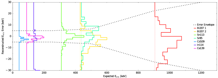
Figure 17: (Color online) The vertical axes appearing at the locations of the expected (i.e., as calculated in Monte Carlo) visible energies (on the horizontal axis) for the various calibration sources show histograms of errors (in keV) in the measured visible energies. The dashed lines then show our conservative estimate of an “error envelope” of the total energy calibration uncertainty based on the widths of the error distributions.

V.10 Visible Energy Reconstruction Uncertainty

The quality of the visible energy calibration procedure was checked by comparing how closely the reconstructed visible energy spectra for the conversion electron calibration sources were aligned with the Monte Carlo predicted spectra. The primary findings of this exercise were:

• For each run, there was an overall $\pm 1.2$% energy uncertainty from gain stabilization.

• At low visible energies (50–100 keV), there was a $\pm 5$% linearity uncertainty, as deduced from a comparison of measured and simulated ¹⁰⁹Cd and ¹³⁹Ce spectra.

• The linearity uncertainty was $\sim 0$ at the ¹¹³Sn peak energy, since this served as an anchor point for the calibrations. At this visible energy range, the visible energy reconstruction error, $\pm 1.7$%, was primarily due to the errors in the position response maps and the run-to-run gain stabilization uncertainty.

• Residual nonlinearity induces a 1.3% ($\sim 10$ keV) error at the $\beta$-decay endpoint energy, based on fits over the visible energy range of 300–700 keV. This is then interpreted as the linearity uncertainty around 500 keV. The linearity uncertainty then increases to $\pm 2.5$% at the upper end of the visible energy range, $\sim 900$ keV, based on the ²⁰⁷Bi upper peak.

Figure 17 shows a histogram of the reconstruction errors in the source peak energies from calibrations across all of the Geometries (A, B, C, and D), together with an “error envelope” of the total calibration uncertainty from the above described sources. Note that this error envelope is a conservative estimate for the uncertainty, based on the widths of the distributions (and is especially conservative at energies below 200 keV, where the envelope is wider than the plotted ¹⁰⁹Cd, ¹³⁹Ce, and ^114mIn distributions), as opposed to the uncertainties in the means. The impact of this uncertainty in the visible energy calibration on the extraction of the $\beta$-asymmetry is discussed later in Section VIII.3.

V.11 Scintillator Trigger Efficiency Functions

An extraction of the scintillator two-fold PMT trigger efficiencies as a function of visible energy was important for comparisons of Monte Carlo calculations with data (especially for backscattering events which deposit small amounts of energy in the scintillator), because the trigger efficiency ultimately impacts the reconstruction of the event type. We extracted these two-fold PMT trigger efficiencies from the measured $\beta$-decay data as a function of the measured visible energy according to the following procedure. First, we employed only electron events satisfying the MWPC position cuts described in Section V.6.2. Second, for every possible pair of two PMTs that both triggered (i.e., generated a signal above pedestal), we then incremented an $E_{\text{vis}}$ “total” histogram for the other two PMTs. For each of the other two PMTs, if it triggered, we then incremented an $E_{\text{vis}}$ “trigger” histogram. Third, the trigger efficiency histogram for each PMT, $\epsilon_{i}$, was then obtained by dividing the “trigger” histogram by the “total” histogram. Finally, the total two-fold PMT trigger efficiency for each scintillator as a function of the visible energy was calculated as [$1-(\text{probability no PMTs trigger})-(\text{probability only one PMT triggers})$], with the appropriate combinatorics for each of the terms in this expression in terms of the individual PMT $\epsilon_{i}$ efficiencies.

The results from such an analysis of the individual PMT efficiencies are shown for one of the detectors in Fig. 18 for one of the Geometries (Geometry C). The PMT efficiency curves for the other detector and the other Geometries were similar. These were incorporated in our Monte Carlo simulation code.

V.12 MWPC Energy Calibration

Figure 18: (Color online) Individual PMT trigger efficiencies $\epsilon_{i}$ for the four PMTs (indicated by the different colors) on one of the detectors, as extracted from an analysis of Geometry C data.

In addition to suppressing gamma-ray backgrounds and permitting the definition of a fiducial volume, Monte Carlo studies suggested that the measured energy deposition in the MWPC on the triggering scintillator side could be used to separate Type 2/3 backscattering events. For example, in the event types schematic shown in Fig. 7, the depicted Type 2/3 events would otherwise appear identical simply in terms of detector signals above threshold. However, in the depicted Type 2 event, the electron traverses the MWPC on the triggering-scintillator side only once, whereas in the depicted Type 3 event, the electron traverses the MWPC on the triggering-scintillator side twice. Therefore, for the Type 2/3 events depicted there, the energy deposition in the MWPC on the triggering-scintillator side would be expected to be greater for the Type 3 event based on path length considerations. Hereafter, we will refer to the MWPC located on the earlier (and the only) triggering-scintillator side as the “Primary MWPC”, and the opposite-side MWPC as the “Secondary MWPC”.

An energy calibration of the MWPC response was performed according to the following procedure. First, we performed polynomial fits to Monte Carlo data of energy deposition in the MWPC for Type 0 neutron $\beta$-decay events (i.e., the calibration was based on Type 0 $\beta$-decay events). Denote the resulting fit function $f_{\text{MC}}(E)$. Second, the MWPC detector face was divided into 10 mm $\times$ 10 mm² square bins (with 88 of these bins providing coverage of the decay trap circular geometry). In each of these 88 bins, we then fitted the function $f_{\text{MC}}(E(x))$, where $x$ denotes the MWPC anode PADC readout channel number, and $E(x)$ was a function (taken to be polynomials) that coverted from channel number to energy. Lookup tables in binned $(x,y)$ positions and anode channel numbers were then constructed for each detector for the different Geometries (i.e., A, B, C, and D).

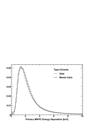
Figure 19: Baseline calibrated Primary MWPC energy spectra for Type 0 neutron $\beta$-decay events from Geometry B (solid line) compared with Monte Carlo calculations (dotted line). The histograms are normalized to unity.

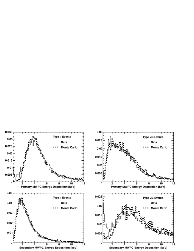
Figure 20: Calibrated Primary (top panels) and Secondary (bottom panels) MWPC energy spectra for Type 1 and Type 2/3 neutron $\beta$-decay events from Geometry B (solid lines) compared with Monte Carlo calculations (dotted lines). The histograms are normalized to unity.

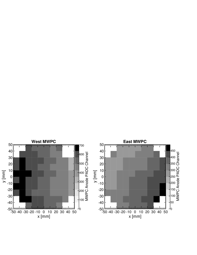
Figure 21: $(x,y)$ position maps of the two MWPCs’ anode PADC channel numbers that correspond to a given calibrated energy (in this case, 4.14 keV).

The quality of the MWPC energy calibration is shown in Figs. 19 and 20. First, in Fig. 19 we compare a baseline calibrated (and background-subtracted) Primary MWPC energy spectrum for Type 0 neutron $\beta$-decay events from Geometry B with Monte Carlo calculations for this Geometry. Recall that the calibration was based on polynomial fits to the Monte Carlo Type 0 (Primary MWPC) spectra. Second, in Fig. 20 we compare calibrated (and background-subtracted) Primary and Secondary MWPC energy spectra for Type 1 and Type 2/3 neutron $\beta$-decay events from Geometry B with Monte Carlo calculations. Note that the Type 1 Primary and Secondary and the Type 2/3 Secondary spectra provide a pseudo-independent check of the calibration, as the Monte Carlo calculations were based on fits to the Type 0 MWPC Primary spectrum (i.e., the spectrum on the earlier, or only, triggering-scintillator side). Note that the calibrated response exhibited a strong position dependence, which can be seen in Fig. 21, where we show position maps of the two MWPCs’ anode channel numbers that correspond to a particular fixed energy (for this plot, 4.14 keV, the relevance of which for the separation of Type 2/3 events is discussed later in Section VI.1.2).

V.13 MWPC Position-Dependent Efficiency

Figure 22: (Color online) Efficiency for the identification of charged particle events by the MWPC detectors (for a fixed PADC channel number cut) plotted as a function of the measured MWPC energy deposition. The non-step-function behavior of these efficiency curves is a result of the MWPCs’ position-dependent response. Typical results for the East (red circles) and West (blue triangles) detectors from Geometries B and D are shown in the left and right panels, respectively.

As discussed earlier in Section V.5.2, a fixed MWPC PADC channel number cut was used to separate gamma ray and charged particle events (i.e., this cut did not vary with the reconstructed $(x,y)$ position). If the MWPC response was independent of position, a plot of the MWPC efficiency for the identification of charged particles as a function of the measured MWPC energy deposition would exhibit a step function at the cut energy (or PADC channel number cut). However, as just shown in Fig. 21, the MWPC response was strongly position-dependent; therefore, for some given energy deposition in the MWPC, the identification of an event as either a gamma ray event or a charged particle event was subject to the MWPCs’ position-dependent response.

The extracted position-dependent efficiency for the identification of charged particle events is illustrated in Fig. 22, where we have plotted the fraction of events passing the standard gamma ray PADC channel number cut as a function of the calibrated energy deposition in the two MWPCs for two examples of typical data sets obtained during Geometries B and D. As can be seen there, over a particular range of energy depositions the fraction of events passing this cut varies monotonically from 0.0 to 1.0, as a result of the MWPCs’ position-dependent response. These measured MWPC efficiency curves were incorporated in our Monte Carlo simulation codes. Note that difference between the two MWPCs’ efficiency curves was smallest (greatest) for Geometry B (Geometry D), with the differences for Geometries A and C in between those of Geometries B and D.

The possible impact of this position-dependent efficiency on the identification of gamma ray events (as opposed to a cut on the MWPC’s calibrated energy response) and thus on the measured asymmetry is discussed later in Section VIII.13.

V.14 Initial Energy Reconstruction

The initial energy of the electron, hereafter denoted $E_{\text{recon}}$, was reconstructed from the measured visible energy in the scintillator based on the results of GEANT4 Monte Carlo simulations for the relation between the measured visible energy in the scintillator, $E_{\text{vis}}$, and the actual initial energy of the emitted $\beta$-decay electron. Parametrizations relating $E_{\text{recon}}$ to $E_{\text{vis}}$ were constructed for the different event types (Type 0, Type 1, and Type 2/3) and for the different Geometries (A, B, and C/D). These parametrizations were based on GEANT4 simulations of conversion electron source spectra, and were extracted from fits of the predicted mean value for $E_{\text{vis}}$ to the true initial source energy, for the various sources employed in the experiment.

Monte Carlo generated source electrons were separated into Type 0, Type 1, and Type 2/3 events, according to the same selection rules as applied in the data analysis. For each Geometry and event type, two different fits were constructed: “Fit 1” was based on the scintillator visible energy, $E_{\text{vis}}$, only; whereas “Fit 2” included both the scintillator visible energy, $E_{\text{vis}}$, and the calibrated MWPC energy, $E_{\text{MWPC}}$. The input variables to the fits were the mean values of: (1) the effective true source energy, $E_{\text{true}}^{\text{source}}$, which accounted for the difference between the Monte-Carlo-generated initial $\beta$-decay energy and the electron’s subsequent energy loss in the 3.6-$\mu$m thick source enclosure foils; (2) the scintillator visible energy, $E_{\text{vis}}$, summed over both scintillators, which accounted for possible sub-trigger-threshold energy deposition in one of the scintillators (e.g., in Type 2/3 events); and (3) the MWPC energy deposition, $E_{\text{MWPC}}$, summed over both MWPCs. For Type 0 and Type 1 events, the functional forms for the fits of $E_{\text{recon}}(\equiv E_{\text{true}}^{\text{source}})$ to $E_{\text{vis}}$ and $E_{\text{MWPC}}$

$$E_{\text{recon}}=\left\{\begin{array}[]{ll}f_{Q}E_{\text{vis}}+\Delta E,&\text{(Fit 1)}\\ f_{Q}E_{\text{vis}}+\Delta E+E_{\text{MWPC}},&\text{(Fit 2)}\end{array}\right.$$ (21)

and for Type 2/3 events

$$E_{\text{recon}}=\left\{\begin{array}[]{ll}\epsilon E_{\text{vis}}^{2}+f_{Q}E_{\text{vis}}+\Delta E,&\text{(Fit 1)}\\ \epsilon E_{\text{vis}}^{2}+f_{Q}E_{\text{vis}}+\Delta E+E_{\text{MWPC}}.&\text{(Fit 2)}\end{array}\right.$$ (22)

For each Geometry, values were fitted for $f_{Q}$, which represented a numerical scintillator quenching factor; $\Delta E$, the energy loss in the decay trap end-cap foils, MWPC windows, etc.; and $\epsilon$, a second-order parameter which was used to control the fits for the Type 2/3 events. The resulting fit parameters are given in Table 5, the point of which serves to set the scale for the Monte Carlo-calculated $\Delta E$ energy loss for the different Geometries.

Figure 23: (Color online) Reconstructions of $E_{\text{recon}}$ values according to the Fit 1 (solid) and Fit 2 (dashed) parametrizations for ¹¹³Sn source calibration Type 0 events from Monte Carlo (thin lines) and experimental data (thick lines). The histograms are normalized to unity.

Table 5: Values of fitted parameters for the $E_{\text{recon}}$ parametrizations. See text for descriptions of parameters. Note that the uncertainties in the fitted parameters were highly correlated; for brevity, we do not report the error matrix here.

Event Type, Fit	Fit Parameter	Geometry A	Geometry B	Geometry C/D
Type 0, Fit 1	$\Delta E$ [keV]	50.7(2)	63.0(2)	33.3(1)
	$f_{Q}$	1.0461(4)	1.0459(4)	1.0476(2)
Type 1, Fit 1	$\Delta E$ [keV]	129(1)	149(1)	73.5(6)
	$f_{Q}$	1.031(2)	1.040(3)	1.035(1)
Type 2/3, Fit 1	$\Delta E$ [keV]	145(8)	152(7)	56(1)
	$f_{Q}$	1.327(56)	1.437(48)	1.420(13)
	$\epsilon$ [keV-1]	$-2.33(65)\times 10^{-4}$	$-3.60(58)\times 10^{-4}$	$-3.26(19)\times 10^{-4}$
Type 0, Fit 2	$\Delta E$ [keV]	45.1(2)	57.4(2)	27.3(1)
	$f_{Q}$	1.0486(4)	1.0484(4)	1.0510(2)
Type 1, Fit 2	$\Delta E$ [keV]	115(1)	136(1)	57.3(9)
	$f_{Q}$	1.031(2)	1.041(3)	1.039(2)
Type 2/3, Fit 2	$\Delta E$ [keV]	121(6)	129(7)	41(1)
	$f_{Q}$	1.276(40)	1.396(53)	1.274(15)
	$\epsilon$ [keV-1]	$-1.88(47)\times 10^{-4}$	$-3.24(64)\times 10^{-4}$	$-1.92(22)\times 10^{-4}$

Figure 23 compares applications of these Fit 1 and Fit 2 parametrizations to $E_{\text{recon}}$ reconstructions of ¹¹³Sn source calibration Monte Carlo and experimental data for Type 0 events. Good agreement between Fits 1 and 2 is observed. In the experimental data, the RMS width of Fit 2 was slightly smaller (by $\sim 2$ keV), suggesting that the inclusion of the MWPC energy slightly improved the resolution. However, we ultimately chose to use Fit 1 instead of Fit 2 for our asymmetry analysis because inclusion of the MWPC energy subjected the value of $E_{\text{recon}}$ to the possibility of an overflow value for the MWPC anode PADC readout (see Fig. 10), which occurred at a calibrated MWPC energy of $\sim 10$ keV. Because we could not reliably construct a value for the MWPC energy in the event of an overflow readout, there was a potential bias in the application of Fit 2 to the data. Nevertheless, the possible impact of this small difference in the Fit 1 and Fit 2 results is discussed later in Section VIII.3.

VI Asymmetry Analysis

In this section we outline our extraction of the asymmetries from the calibrated data. We begin by defining our different Analysis Choices for the extraction of the asymmetries under which we included or excluded the various backscattering event types. Next, we describe our procedure for the extraction of the binned (in energy) background-subtracted event rates (and their statistical uncertainties) from the $\beta$-decay and background runs, and proceed to an extraction of the asymmetries under the octet data-taking sequences via the super-ratio technique discussed earlier. We then show results from a number of basic data quality assessment checks, including comparisons of the reconstructed energy spectra with Monte Carlo results, assessments of the stability of the energy scale with time (as quantified via Kurie fits to the $\beta$-decay endpoints), and assessments of the statistical properties of the asymmetries under the octet data-taking sequence.

Table 6: Definitions of the different Analysis Choices for the inclusion or exclusion of the various backscattering event types, and the selection rules for the assignment of the electron’s initial direction. “Trigger Side” refers to the scintillator generating the trigger.

	Assignment of Initial Direction for Backscattering Event Types
Analysis Choice	Type 0	Type 1	Type 2/3
1	Trigger Side	Earlier Trigger Side	Trigger Side
2	Trigger Side	Earlier Trigger Side	Omit
3 (default)	Trigger Side	Earlier Trigger Side	If Primary $E_{\text{MWPC}}>4.14$ keV Trigger Side, Else Other Side
4	Trigger Side	Omit	Omit
5	Trigger Side	Earlier Trigger Side	Apply Likelihood Function Prob($E_{\text{MWPC}}$) for Assignment of Direction
6	Omit	Earlier Trigger Side	Omit
7	Omit	Omit	Trigger Side
8	Omit	Omit	If Primary $E_{\text{MWPC}}>4.14$ keV Trigger Side, Else Other Side
9	Omit	Omit	Apply Likelihood Function Prob($E_{\text{MWPC}}$) for Assignment of Direction

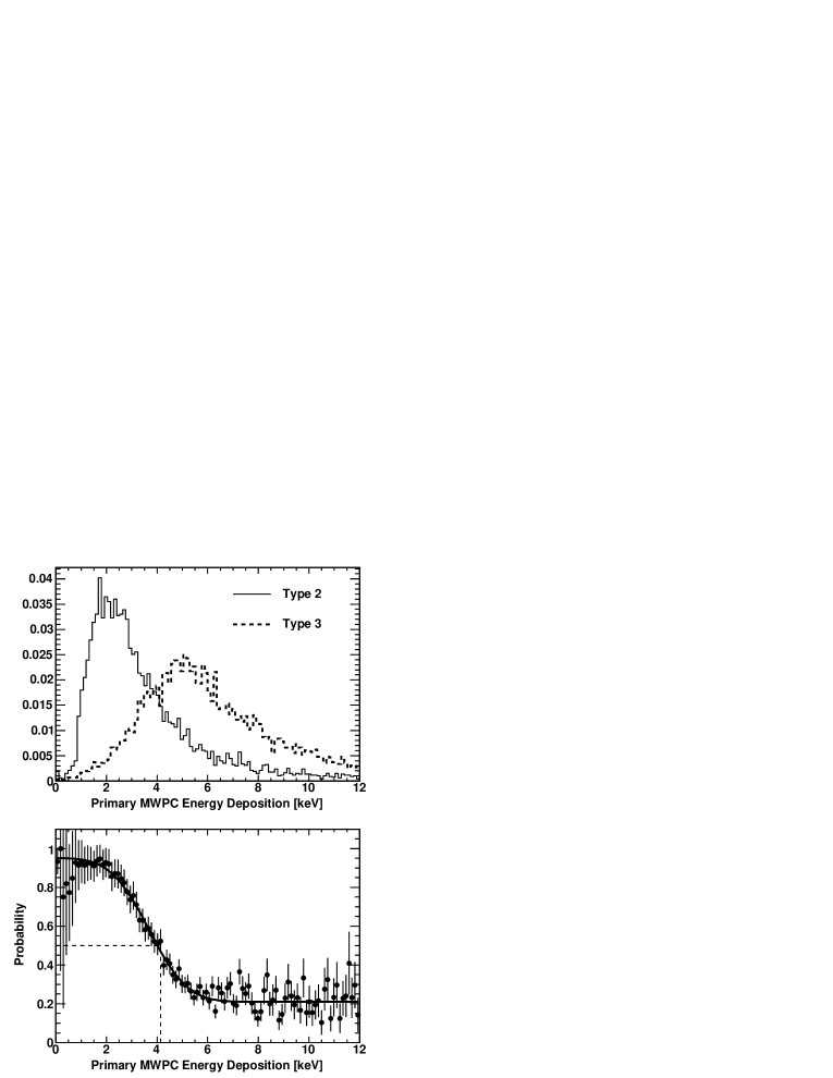
Figure 24: Top panel: Monte Carlo calculations of the energy deposition in the Primary MWPC for Type 2 and Type 3 neutron $\beta$-decay events. The histograms are normalized to unity. Bottom panel: Monte Carlo calculations of the probability an event identified in data analysis as a Type 2/3 event was a Type 2 event as a function of the energy deposition in the Primary MWPC. The dashed lines indicate the threshold cut of $E_{\text{MWPC}}>4.14$ keV for the assignment of the initial direction to the triggering-scintillator side in Analysis Choices 3 and 8 for the separation of Type 2/3 events. The solid line is a fit to the calculations of the form $\text{Prob}(E_{\text{MWPC}})=-p_{0}\text{erf}(p_{1}E_{\text{MWPC}}-p_{2})+p_{3}$, where erf denotes the error function and the $p_{i}$ are fit parameters. This likelihood function was employed for the separation of Type 2/3 events in Analysis Choices 5 and 9.

VI.1 Analysis Choices

VI.1.1 Definitions and Selection Rules

We extracted the asymmetries according to a number of different Analysis Choices under which we included or excluded the various backscattering event types and varied the selection rules for the assignment of the electron’s initial direction. The motivation for this study was to compare the variation of the measured asymmetry as a function of the analysis choice with the variation predicted by the Monte Carlo as a robust benchmark of our Monte-Carlo-calculated corrections for backscattering and the $\cos\theta$-dependence of the acceptance.

The selection rules for our various Analysis Choices, numbered 1–9, are summarized in Table 6. Note that Analysis Choices 1–5 consider Type 0 events, with different selections for the inclusion/exclusion of Type 1 and 2/3 events, and further selection rules for the identification of the initial direction of incidence for Type 2/3 events. Analysis Choices 6–9 were included in order to study the asymmetry from backscattering events for diagnostic purposes.

We employed Analysis Choice 3 as our default method for the extraction of our final results for $A_{0}$, because this choice provided for maximal use of detector information and minimized the magnitude of the systematic corrections for backscattering and the $\langle\cos\theta\rangle$ dependence of the acceptance. Nevertheless, we show several results from the other Analysis Choices below, as these results provide a powerful validation of our Monte Carlo calculations.

VI.1.2 Treatment and Separation of Type 2 and Type 3 Events

Note that in Analysis Choices 1 and 7 we assigned the initial direction of incidence for Type 2/3 events simply to the triggering-scintillator side. However, we attempted in Analysis Choices 3, 5, 8, and 9 to separate Type 2 and 3 events according to selection rules on the energy response of the Primary MWPC (i.e., recall, the MWPC on the triggering scintillator side). To illustrate, the top panel of Fig. 24 shows Monte Carlo calculations of the energy deposition in the Primary MWPC for Type 2 and Type 3 neutron $\beta$-decay events separately (of course, such a direct separation was not possible in data analysis). The distinct spectra for these events suggested such a separation could be performed via a probabilistic (likelihood) approach, and the feasilibity of such was studied in Monte Carlo. Results from this study are shown in the bottom panel of Fig. 24, where calculations of the probability that an event identified in data analysis as a Type 2/3 event was actually a Type 2 event are plotted as a function of $E_{\text{MWPC}}$.

The $E_{\text{MWPC}}>4.14$ keV energy cut employed in Analysis Choices 3 and 8 was chosen such that if a fixed Primary MWPC energy cut was used to assign the initial direction of incidence for events identified as Type 2/3 in data analysis to either the triggering-scintillator side or the non-triggering-scintillator side, the calculated probability for the incorrect assignment of the initial direction to the triggering scintillator side was less than 50% (i.e., the calculated probability that the event was actually a Type 2 event). This threshold cut is consistent with the conceptual expectation (see, e.g., Fig. 7) that an observed Type 2/3 event which was actually a Type 2 event (i.e., initially incident on the non-triggering-scintillator side) would deposit less energy in the Primary MWPC (one traversal) as compared to a Type 3 event (two traversals).

In Analysis Choices 5 and 9 we then actually separated the Type 2/3 events according to the calculated likelihood function Prob($E_{\text{MWPC}}$), such as that already shown in the bottom panel of Fig. 24. (Note that although the curve shown there is from a Monte Carlo calculation for the Geometry A configuration, the curves for the other Geometries were similar.) Fig. 25 then demonstrates the good agreement observed between the data and Monte Carlo for the Primary MWPC energy spectra for Geometry A Type 2 and Type 3 events, separated according to the likelihood function.

Figure 25: (Color online) Comparison between data (red triangles) and Monte Carlo (filled squares) for Primary MWPC energy spectra for Geometry A Type 2 and Type 3 events, after separation of Type 2/3 events in data analysis according to the likelihood function Prob($E_{\text{MWPC}}$).

VI.2 Event Rates and Statistical Uncertainties

For any given Analysis Choice, events were binned into 25 keV $E_{\text{recon}}$ energy bins from 0–1200 keV, and then assigned an initial direction of incidence according to the selection rules in Table 6. The measured event rate in each of these $E_{\text{recon}}$ bins was then computed for each detector according to

$$r_{\text{bin}}=\frac{N_{\text{bin}}}{T},$$ (23)

where $N_{\text{bin}}$ denotes the number of events passing cuts in that particular $E_{\text{recon}}$ bin, and $T$ denotes that detector’s live time (defined previously in Section V.4).

In energy bins containing $N<20$ counts (e.g., in bins beyond the $\beta$-decay endpoint for $\beta$-decay runs, or in nearly all bins for the shorter background runs), where the assumption of Gaussian errors approximated by Poisson uncertainty is no longer valid, we assigned a statistical uncertainty to the rate in these bins according to the following procedure whose key assumption was that the underlying background and neutron $\beta$-decay spectral shapes did not change with time, even if the run-by-run rates varied.

First, we generated high-statistics parent $\beta$-decay and background spectra for each of the detectors (for a particular Geometry and spin state) by combining many runs. Second, on an individual run-by-run basis, we then computed the measured rate for each detector within an energy window, $r^{\text{meas}}_{\text{window}}$, nominally 275–625 keV (see Section VII.6), and compared this measured rate with the rate for the parent spectrum, $r^{\text{parent}}_{\text{window}}$, in this same energy window. Third, the ratio of these two rates then defined a scaling factor $f\equiv r^{\text{meas}}_{\text{window}}/r^{\text{parent}}_{\text{window}}$ for each of the detectors, which we then used to compute on a run-by-run basis the expected rate for each energy bin, $r^{\text{exp}}_{\text{bin}}=r^{\text{parent}}_{\text{bin}}\times f$, for each detector. Finally, the statistical uncertainty we then assigned to the measured rate in each bin was then

$$\delta r_{\text{bin}}=\sqrt{\frac{r^{\text{exp}}_{\text{bin}}}{T}},$$ (24)

where $T$ again denotes that particular detector’s (blinded) live time. For bins with $\geq 20$ counts, we employed the usual $\sqrt{N}$ uncertainties.

For each $\beta$-decay and background run pair, we then subtracted on a bin-by-bin basis the measured background rate from the measured $\beta$-decay rate, with standard propagation of the statistical errors calculated according to the above-described procedure for $N<20$ or $N\geq 20$ counts. We emphasize that this procedure affected only the assignment of the statistical errors; the actual measured counts were still employed for the calculation of the run-by-run rates for each $\beta$-decay and background run pair.

VI.3 Asymmetry Extraction

We then extracted the experimental asymmetry on an energy-bin-by-energy-bin basis for data grouped into either individual spin-state run pairs, quartets, or octets (all of which were defined previously in Section IV.1.1).

VI.3.1 Spin-State Pair Asymmetries

For individual spin-state run pairings (i.e., A1–A6, A7–A12, B1–B6, or B7–B12 run pairings in Table 2), we calculated the experimental measured asymmetries according to the definition for the super-ratio of detector rates given previously in Eq. (10),

$$R=\frac{r_{1}^{-}\cdot r_{2}^{+}}{r_{1}^{+}\cdot r_{2}^{-}},~{}~{}~{}~{}~{}A_{\text{meas}}=\frac{1-\sqrt{R}}{1+\sqrt{R}}.$$ (25)

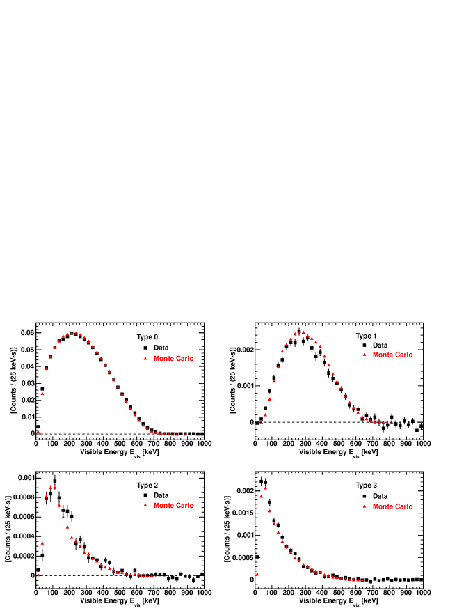
Figure 26: (Color online) Comparisons of visible energy spectra for the different event types extracted from data (black squares) and Monte Carlo (red triangles) for the Geometry C configuration. The same selection rules for the event types were applied to both data and Monte Carlo. See text for details. All error bars shown are statistical; if not visible, the errors are smaller than the marker size.

Figure 27: Fractional residuals for the comparisons between the data and Monte Carlo visible energy spectra shown in Fig. 26. As can be seen in Fig. 26, there are very few Type 2 and Type 3 events with visible energies greater than $\sim 500$ keV.

VI.3.2 Quartet Asymmetries

Conceptually, the asymmetry for a quartet run pairing (i.e., either A-type A1–A12 or B-type B1–B12 runs in Table 2) can be computed from a “summed super ratio” of detector rates,

$$R^{\prime}=\frac{[r_{1}^{-(\text{A1,A2})}+r_{1}^{-(\text{A10,A12})}]\cdot[r_{2}^{+(\text{A4,A5})}+r_{2}^{+(\text{A7,A9})}]}{[r_{1}^{+(\text{A4,A5})}+r_{1}^{+(\text{A7,A9})}]\cdot[r_{2}^{-(\text{A1,A2})}+r_{2}^{-(\text{A10,A12})}]},$$ (26)

where the notation is such that the run pairs within ($\cdots$) parentheses indicate the $\beta$-decay run and ambient background run background-subtraction pairing. The expression for B-type runs is similar. The merit of this approach is that that linear background and detector efficiency drifts cancel in this definition of $R^{\prime}$. (This cancellation is exact provided that the durations of the $\beta$-decay and background runs do not vary and that any such linear drifts are constant in time.)

In practice, to properly account for the statistical uncertainty, within each quartet we computed the statistically weighted mean of the detector rates for each of the polarization states. The resulting statistical uncertainties in the mean rates were then propagated into the super ratio $R^{\prime}$ and then into the calculation of the asymmetry. For example, we defined the detector rate $r_{1}^{+}$ for an A-type quartet to be the statistically weighted mean of the $r_{1}^{+(\text{A1,A2})}$ and $r_{1}^{+(\text{A10,A12})}$ rates. The quartet-based asymmetry was then extracted from the super ratio $R^{\prime}$ of these quartet-averaged rates.

Note that a “product super ratio”, $R^{\prime\prime}$, can also be defined in terms of geometric means of detector rates for spin states as

$$R^{\prime\prime}=\left[\frac{[r_{1}^{-(\text{A1,A2})}r_{1}^{-(\text{A10,A12})}]\cdot[r_{2}^{+(\text{A4,A5})}r_{2}^{+(\text{A7,A9})}]}{[r_{1}^{+(\text{A4,A5})}r_{1}^{+(\text{A7,A9})}]\cdot[r_{2}^{-(\text{A1,A2})}r_{2}^{-(\text{A10,A12})}]}\right]^{1/2}.$$ (27)

We extracted asymmetries via both the summed and product super-ratio approaches, and the central values from the two methods differed by only 0.07%. However, the problem with the product super-ratio method is that the resulting statistical uncertainty in $R^{\prime\prime}$ is dominated by the rate from the run with the largest statistical uncertainty (e.g., if one of the $\beta$-decay runs is significantly shorter in duration than the others). In contrast, the summed super-ratio method employs inverse-square-uncertainty weighting. Therefore, in our final analysis we employed the summed super-ratio method.

VI.3.3 Octet Asymmetries

Octet-based asymmetries were calculated similarly to quartet-based asymmetries. Now, for example, we defined the detector rate $r_{1}^{+}$ for a complete octet to be the statistically weighted mean of the $r_{1}^{+(\text{A1,A2})}$, $r_{1}^{+(\text{A10,A12})}$, $r_{1}^{+(\text{B4,B5})}$, and $r_{1}^{+(\text{B7,B9})}$ rates. As with the quartet-based asymmetry, the octet-based asymmetry was then extracted from a summed super-ratio $R^{\prime}$ of these octet-averaged rates, with propagation of the statistical uncertainties in the octet-averaged rates through the super ratio and the asymmetry. Again, the merit of the octet approach is that linear background drifts cancel (subject to the same caveats as for the quartet asymmetries).

VI.4 Comparison of Data and Monte Carlo Visible Energy Spectra

VI.4.1 Visible Energy Spectra

We now show an example (for the entire Geometry C data set) of comparisons of the measured background-subtracted visible energy $E_{\text{vis}}$ spectra with results from Monte Carlo (GEANT4 except where noted) calculations (assuming the Particle Data Group value for $A_{0}$) in Fig. 26 for the different event types. The fractional residuals, (Data $-$ Monte Carlo)/Data, are shown in Fig. 27. Although not shown explicitly in this article, we note that we achieved the same level of agreement between data and Monte Carlo shown in Fig. V.14 for all of the Geometries and both detectors.

Both the measured and Monte Carlo data shown there were extracted from events triggering one of the particular scintillators. Type 2/3 events were separated in both data and Monte Carlo according to the selection rules of Analysis Choice 3. The Type 0, Type 2, and Type 3 $E_{\text{vis}}$ spectra shown there are the spectra observed in the triggering scintillator, whereas the Type 1 spectra are summed over both of the scintillators.

The spectra shown there are for one of the neutron spin states (in particular, AFP spin-flipper off). Note that the total measured background-subtracted rate during runs when the neutron spin was flipped with the AFP spin-flipper was $\sim 30$% less than that during runs for the unflipped spin state, due to UCN losses along the transport guides between the AFP spin-flip region and the SCS decay-trap volume after the 2-T equivalent UCN energy increase following the spin flip.

VI.4.2 Backscattering Strengths and Fractions

The normalization of the measured and Monte Carlo (GEANT4) spectra shown in Fig. 26 was performed according to their respective integral of the Type 0 spectrum over the complete visible energy range of 0–800 keV. After this relative normalization, the GEANT4 spectra were further internally normalized to account for a known deficit in the GEANT4 backscattering strength martin03 ; martin06 . This was accomplished by applying two scale factors, $f_{\text{bulk}}$ (for backscattering from the scintillator bulk material) and $f_{\text{thin}}$ (decay trap and MWPC thin windows), to the GEANT4 backscattering distributions such that the simulated backscattering strengths matched the measured backscattering strengths. Specifically, we applied $f_{\text{bulk}}$ to Type 1 and Type 3 events, whereas we applied $f_{\text{thin}}$ to Type 2 events, because the former (latter) correspond to backscattering from the bulk scintillator (MWPC windows, gaseous materials, etc.). The numerical values of these scale factors were $f_{\text{bulk}}=1.3$ for all of the Geometries, and $f_{\text{thin}}=1.3$ (1.6) for Geometries A and B (C and D). The Type 1, Type 2, and Type 3 Monte Carlo spectra shown in Fig. 26 are scaled by these scale factors.

For completeness, the measured event type fractions integrated over the entire visible energy range from 0–800 keV for the different Geometries are tabulated in Table 7.

Table 7: Measured event type fractions for each Geometry integrated over the entire visible energy range from 0–800 keV and averaged over the detectors and the spin states. Type 2/3 events were separated according to Analysis Choice 3.

Geometry	Type 0	Type 1	Type 2	Type 3
A	0.947	0.032	0.011	0.011
B	0.952	0.030	0.010	0.008
C	0.930	0.047	0.009	0.014
D	0.939	0.039	0.008	0.014

VI.5 Fitted Endpoint Distributions

Figure 28: Example of a Kurie fit to the (background-subtracted) reconstructed energy $E_{\text{recon}}$ spectrum for a $\sim 1$-hour long $\beta$-decay run. The errors shown are statistical.

As a measure of the stability of the energy calibration with time, background-subtracted $E_{\text{recon}}$ spectra for each $\beta$-decay run were converted to Kurie plots and fitted over the range of 400–700 keV. An example of such a fit to the $E_{\text{recon}}$ spectrum from a $\sim 1$-hour long $\beta$-decay run is shown in Fig. 28. There, we fitted the measured rate, binned in energy, $dW/dE_{e}$, to the function

$$\frac{1}{p_{e}}\sqrt{\frac{dW}{dp_{e}}}=\frac{1}{p_{e}}\sqrt{\frac{dW}{dE_{e}}\frac{dE_{e}}{dp_{e}}}\propto(T_{0}-T_{e}),$$ (28)

where $T_{0}$ denotes the fitted endpoint (kinetic) energy, $p_{e}=\sqrt{T_{e}^{2}+2T_{e}m_{e}}$ is the magnitude of the electron momentum, $T_{e}$ ($=E_{\text{recon}}$) is the kinetic energy, and $dE_{e}/dp_{e}=p_{e}/E_{e}=p_{e}/(T_{e}+m_{e})$.

Fits to Kurie plots of Monte Carlo spectra for the two spin states (in order to account for the $\beta\cos\theta$ factor in the angular distribution) which included the energy-dependent recoil order effects and the finite scintillator energy resolution yielded fitted values for the endpoint of $\sim 787$ keV (with a $\sim\pm 0.4$ keV difference for the two spin states).

Distributions of fitted endpoints for the two detectors (employing “Fit 1” for the $E_{\text{recon}}$ reconstruction), summed over all Geometries and spin states and weighted by the inverse square of their statistical uncertainties are shown in Fig. 29. For both detectors, typical run-to-run fluctuations (as characterized by the RMS) were less than $\sim 13$ keV. However, there was a systematic $\sim 10$–14 keV difference between the mean fitted endpoints and the Monte Carlo result of $\sim 787$ keV, which is addressed later in Section VIII.3.

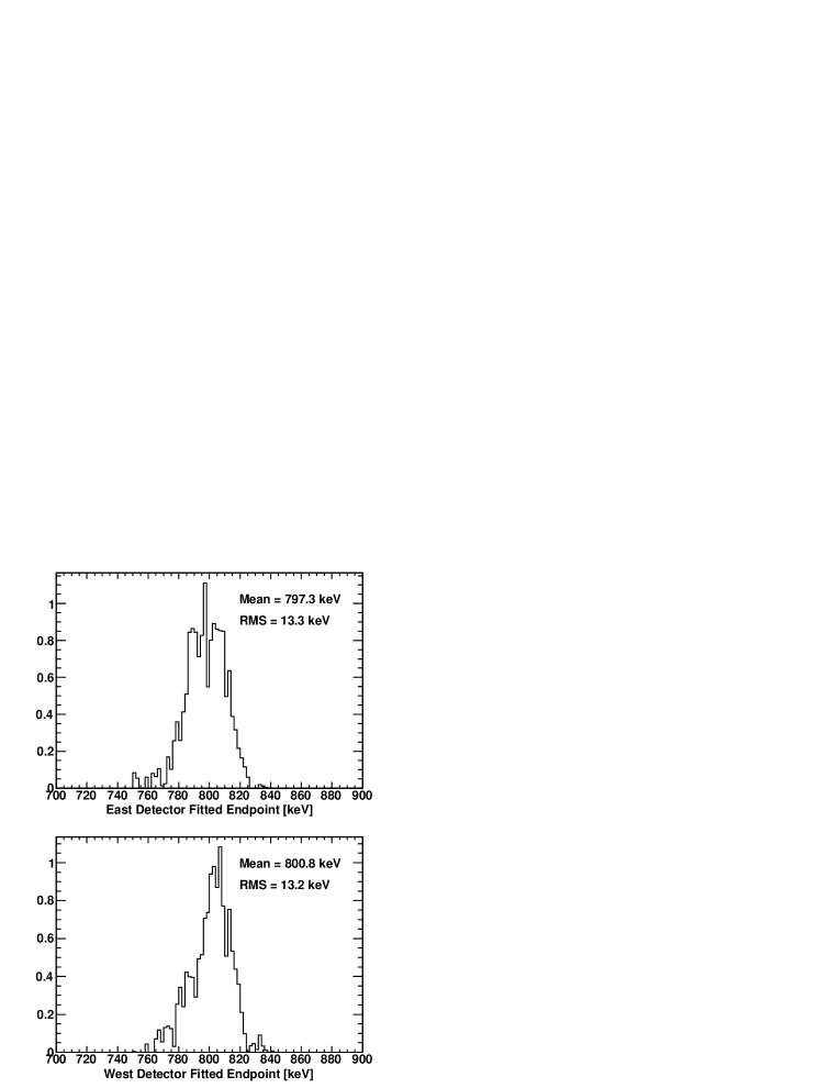
Figure 29: Distributions of fitted endpoints for the two detectors, averaged over Geometries and spin states. The histogram contents were weighted by the inverse square of their uncertainties.

VI.6 Statistical Properties of the Asymmetries

Figure 30: Extracted values for the (blinded) measured asymmetries, $A_{\text{meas}}$, from the Geometry B data set obtained under Analysis Choice 3 for spin-state run pairings (top panel), quartet run pairings (middle panel), and octet run pairings (bottom panel).

As a demonstration of the utility of our octet data-taking procedure, we extracted values for the measured blinded asymmetries, $A_{\text{meas}}$, under Analysis Choice 3 integrated over a 225–675 keV energy window for the three different run groupings discussed previously: spin-state pairs, quartets, and octets. Incomplete octets were not discarded; instead, we retained individual spin-state pairs or quartets within incomplete octets in our analysis.

Sample results from an analysis of the Geometry B data set are shown in Fig. 30. As can be seen there, the $\chi^{2}/\nu$ value for the quartet analysis is improved over that for the spin-state pair analysis. Further, there is a slight shift in the central value of the asymmetry between the spin-state pair analysis and the quartet analysis. If there were linear drifts in the backgrounds and/or detector efficiencies, this is the expected result, as any such linear drifts would bias the spin-state pair analysis, but would cancel in the quartet analysis. In comparing all of the Geometries, the $\chi^{2}/\nu$ values for the octet analyses of Geometries A, B, C, and D were 30.1/29, 12.8/22, 20.1/13, and 6.5/7, respectively (i.e., the relatively small $\chi^{2}/\nu$ value for Geometry B was not representative of the entire data set).

All of the asymmetry results presented hereafter were obtained under the octet analysis.

VII Systematic Corrections for $\bm{A_{0}}$ Extraction

In this section we discuss the systematic corrections for backscattering, the $\cos\theta$-dependent acceptance (hereafter also termed the “angle effect”), and the Standard Model recoil-order and radiative corrections that were applied to the measured asymmetries in order to extract the desired $\beta$-asymmetry parameter $A_{0}$. The Monte Carlo corrections for the backscattering and angle effect corrections presented here were based on our GEANT4 Monte Carlo simulation code. However, as noted earlier, we also developed a PENELOPE simulation code and, in general, we obtained good agreement between the GEANT4- and PENELOPE-calculated corrections. The small differences between the results from these two simulation programs are discussed in the context of the systematic uncertainty for the backscattering and $\cos\theta$-dependent acceptance corrections later in Section VIII.12.

VII.1 Monte Carlo Benchmark: Scaling of Asymmetries with Analysis Choice

First, as a benchmark of the validity of our Monte Carlo treatment of the angle and backscattering effects, we demonstrate that the scaling of our (still-blinded) measured asymmetries, $A_{\text{meas}}$, with the Analysis Choice (calculated according to the selection rules in Table 6) is consistent with our Monte Carlo predictions. An example of this is shown in Fig. 31, where we have plotted the (blinded) measured asymmetries $A_{\text{meas}}$ and both the GEANT4 and PENELOPE Monte Carlo predictions for $A_{\text{meas}}$, integrated over an energy window of 225–675 keV, as a function of the Analysis Choice for each of the Geometries. Note that the Monte Carlo predictions shown there were arbitrarily scaled (for effectively an arbitrary $A_{0}$) in order to match the data at Analysis Choice 3 (given that the measured asymmetries shown there were blinded); the point of this exercise was to demonstrate that the scaling of the Monte Carlo-calculated asymmetries with the Analysis Choice matched that of the measured asymmetries. [An absolute comparison would have required scaling each by the (unknown) unblinded values of $A_{0}$ for each Geometry.]

Figure 31: Comparison of the scaling of the (blinded) measured asymmetries extracted from the data, $A_{\text{meas}}$, and the Monte Carlo-calculated asymmetries (from both GEANT4 and PENELOPE) with the Analysis Choice for each of the Geometries. The asymmetries shown here were integrated over an energy window of 225–675 keV. The results from the Monte Carlo calculations were scaled for each Geometry in order to match the data at Analysis Choice 3. All errors are statistical, with the GEANT4 statistical errors smaller than the symbol size.

This agreement between the scaling of our measured and Monte-Carlo-calculated results for $A_{\text{meas}}$ with the Analysis Choice (and, thus, upon the inclusion or exclusion of the different backscattering event types, with different selection rules therein for identification of the backscattering event types) provides a powerful demonstration of the validity of our Monte Carlo-calculated corrections for backscattering and the $\cos\theta$-dependence of the acceptance, and also validates our application of the scale factors $f_{\text{bulk}}$ and $f_{\text{thin}}$ to the GEANT4 backscattering distributions, discussed previously in Section VI.4.2.

Hereafter, all of the results shown for the asymmetries and the Monte Carlo-calculated systematic corrections to the asymmetries were obtained under the default Analysis Choice 3, the motivation for which was noted previously in Section VI.1.1.

VII.2 Asymmetry Unblinding

All of the asymmetry results shown hereafter constitute our final (unblinded) results. We note that during our actual analysis of the blinded data, we did not unblind our asymmetries until after all of the (already discussed) calibrations and cuts, the systematic corrections and uncertainties now being discussed, and the analysis energy window (discussed later in Section VII.6) were finalized. At that time, the asymmetries were unblinded by removing the scale factors applied to the detector rates which were used to blind the data (as discussed previously in Section V.3).

We emphasize that our final results for $A_{0}$ presented later were those obtained at the time the data were unblinded; no further data analysis was conducted after the unblinding.

VII.3 Results for Measured Asymmetries

Our resulting measured asymmetries, $A_{\text{meas}}(E_{\text{recon}})$, are shown in Fig. 32 as a function of $E_{\text{recon}}$ in 25 keV bins over the entire detectable energy range, 50–800 keV, for each of the Geometries. There, we also show for each Geometry the measured background spectrum and the resulting bin-by-bin background-subtracted $\beta$-decay spectrum.

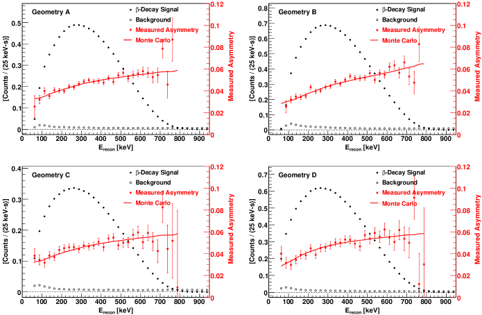
Figure 32: (Color online) Results for the measured background $E_{\text{recon}}$ energy spectra (open circles) and the background-subtracted neutron $\beta$-decay $E_{\text{recon}}$ energy spectra (filled circles) for each of the Geometries. The spectra shown here were summed over both detectors and then averaged over the two neutron spin states. The resulting measured asymmetries $A_{\text{meas}}$ (filled red squares; see vertical scale on the right) are shown as a function of $E_{\text{recon}}$ for each of the Geometries. These are compared with the Monte Carlo calculated values for the measured asymmetries (solid red lines). The energy dependence of the measured asymmetries is primarily due to the $\beta\cos\theta$ dependence of the measured asymmetries [see Eq. (8)]; there are also $\langle\beta\cos\theta\rangle$ acceptance and backscattering effects (e.g., compare Geometry B). All errors are statistical.

VII.4 Overview of Method for Systematic Corrections to Extract $\bm{A_{0}}$

For a given energy bin in “true initial energy”, the true energy-dependent physics asymmetry under the Standard Model would be $P_{n}A_{0}\langle\beta_{\text{true}}\cos\theta\rangle(1+f_{\text{RO}})$, where $P_{n}$ is the neutron polarization, $\langle\beta_{\text{true}}\cos\theta\rangle$ denotes the average value of the product of the true electron velocity in units of $c$ with the true electron pitch angle $\cos\theta$ for that energy bin, and $f_{\text{RO}}$ denotes the (energy-dependent) recoil-order physics correction to $A_{0}$. For now, we have omitted the small $\mathcal{O}(0.1\%)$ radiative correction to the asymmetry discussed in the Introduction to this article.

Therefore, it is clear that an extraction of the desired $\beta$-asymmetry parameter $A_{0}$ from the (energy-dependent) measured asymmetry $A_{\text{meas}}(E_{\text{recon}})$ in each $E_{\text{recon}}$ bin requires a correct reconstruction of the mean (initial) energy in each energy bin, a correction to the measured asymmetry for missed backscattering, and a calculation of the mean value of $\langle\beta_{\text{recon}}\cos\theta\rangle$ in that energy bin. For now, we will assume that in each particular energy bin $\langle E_{\text{recon}}\rangle=\langle E_{\text{true}}\rangle$, or $\langle\beta_{\text{recon}}\rangle=\langle\beta_{\text{true}}\rangle$; later, we will explore the implication for a systematic uncertainty to the asymmetry resulting from a possible $E_{\text{recon}}\neq E_{\text{true}}$ error, such as from an energy calibration error. Note that even under the assumption that $E_{\text{recon}}=E_{\text{true}}$ (i.e., “perfect” calibration), an acceptance correction must still be applied for the average value of $\langle\beta\cos\theta\rangle$ in each energy bin, because the electron energy loss (in the decay trap end-cap foils, MWPC windows, etc.) is strongly angle dependent (hence the designation “angle effect”), with the energy loss a monotonically increasing function of the pitch angle. Therefore, each $E_{\text{recon}}$ bin includes a distribution of events in initial true energy and pitch angle.

We used our Monte Carlo simulation code to compute these required corrections for missed backscattering and the $\langle\beta\cos\theta\rangle$ angle effect. After extraction of the measured asymmetry $A_{\text{meas}}(E_{\text{recon}})$ in each $E_{\text{recon}}$ energy bin, we then applied the following corrections in a sequential manner in order to extract $A_{0}$ from $A_{\text{meas}}(E_{\text{recon}})$:

VII.4.1 Asymmetry Energy Dependence and $\beta$-Decay Spectra

(1) First, we made a first-order bin-by-bin correction for the energy-dependence of the measured asymmetries, $A_{\text{meas}}(E_{\text{recon}})$, by calculating an asymmetry $A_{1}(E_{\text{recon}})$, defined by

$$A_{1}(E_{\text{recon}})\equiv A_{\text{meas}}/(\frac{1}{2}\beta_{\text{recon}}),$$ (29)

where $\beta_{\text{recon}}$ was calculated for the central value of each $E_{\text{recon}}$ bin for each event class. Note that this first-order correction simply assumed a uniform value (or distribution) of $\beta_{\text{recon}}$ within each energy bin, and also a symmetric value for $\langle\cos\theta\rangle$ of 1/2 in each energy bin.

VII.4.2 Backscattering Corrections

(2) Second, we applied a bin-by-bin correction for missed (or misidentified) backscattering events, with the result of this correction $A_{2}(E_{\text{recon}})$ defined to be

$$A_{2}(E_{\text{recon}})\equiv A_{1}(E_{\text{recon}})(1+\Delta_{2}),$$ (30)

where $\Delta_{2}\equiv\Delta_{2,0}+\Delta_{2,1}+\Delta_{2,2}$ represents the total backscattering correction in each $E_{\text{recon}}$ bin, which we define to be the sum of the individual corrections for events misidentified as Type 0, Type 1, and Type 2/3 events, respectively. The fractional correction factors $\Delta_{2,i}$ were extracted from Monte Carlo.

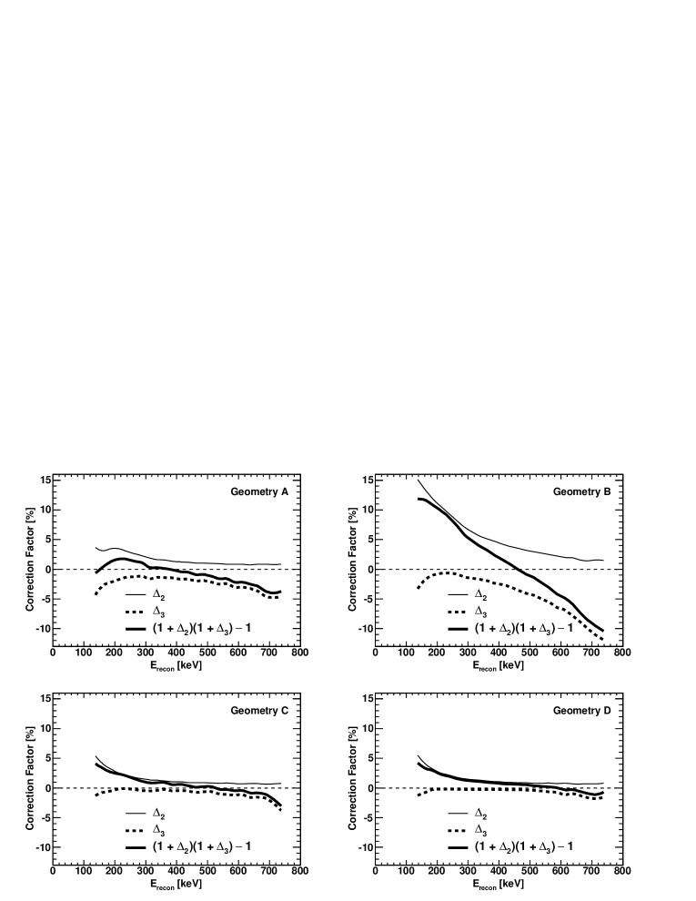
Figure 33: Results from GEANT4 Monte Carlo calculations of the energy dependence of the relative sizes of the $\Delta_{2}$ backscattering (thin solid line) and $\Delta_{3}$ angle effect (thick dashed line) systematic corrections. The energy dependence of the relative size of the combined correction $(1+\Delta_{2})(1+\Delta_{3})$ is then shown as the thick solid line. The systematic uncertainties in these calculations are discussed in detail later in Section VIII.12.

VII.4.3 $\langle\beta\cos\theta\rangle$ Acceptance Corrections

(3) Third, for each event class we applied a bin-by-bin correction for the $\langle\beta\cos\theta\rangle$ angle effect, with the result of this correction $A_{3}(E_{\text{recon}})$ defined to be

$$A_{3}(E_{\text{recon}}) = A_{2}(E_{\text{recon}})\times\frac{1}{2}\beta_{\text{recon}}/\langle\beta_{\text{true}}\cos\theta\rangle$$ (31)

$$\equiv A_{2}(E_{\text{recon}})(1+\Delta_{3}).$$

Again, the fractional correction factors $\Delta_{3}$ were extracted from Monte Carlo.

VII.4.4 Standard Model Corrections

(4) After application of the above three corrections, the resulting asymmetry $A_{3}(E_{\text{recon}})$ is proportional to the product of $P_{n}$, $A_{0}$, and the (energy-dependent) recoil-order and radiative corrections (which are calculable under the Standard Model). As a final step, we extracted a value for $A_{0}$ in each $E_{\text{recon}}$ bin according to

$$A_{0}(E_{\text{recon}})/P_{n}=$$

$$~{}~{}~{}~{}~{}A_{3}(E_{\text{recon}})[1+\Delta_{\text{RO}}(E_{\text{recon}})][1+\Delta_{\text{rad}}(E_{\text{recon}})],$$

where $\Delta_{\text{RO}}(E_{\text{recon}})$ and $\Delta_{\text{rad}}(E_{\text{recon}})$ denote the energy-dependent recoil-order and radiative corrections, respectively, for that particular $E_{\text{recon}}$ bin. In the absence of new physics, there should be no residual energy dependence to the values of the asymmetries $A_{0}(E_{\text{recon}})$ extracted from all of the $E_{\text{recon}}$ bins after application of these Standard Model corrections; therefore, the final energy-averaged value for $A_{0}$ will be the statistically-weighted average of the bin-by-bin $A_{0}(E_{\text{recon}})$ values,

$$A_{0}=\langle A_{0}(E_{\text{recon}})\rangle.$$ (33)

We now describe the results from our Monte Carlo calculations of the $\Delta_{2,i}$ and $\Delta_{3}$ correction factors in more detail.

VII.5 Results for Monte Carlo Corrections

Figure 34: Results from GEANT4 Monte Carlo calculations of the relative sizes of the individual $\Delta_{2,0}$ (thin solid line), $\Delta_{2,1}$ (thick solid line), and $\Delta_{2,2}$ (thick dashed line) contributions to the total $\Delta_{2}$ backscattering systematic correction. The systematic uncertainties in these calculations are discussed in detail later in Section VIII.12. [The $\Delta_{2,1}$ backscattering correction is non-zero because some small fraction of events will initially backscatter from the decay-trap end-cap foils, and then undergo Type 1 backscattering (however, the reconstructed initial direction will then be incorrect). The probability for this type of event increases with decreasing energy, and thus the acceptance for this type of events was suppressed in Geometries A and B (i.e., thicker MWPC windows).]

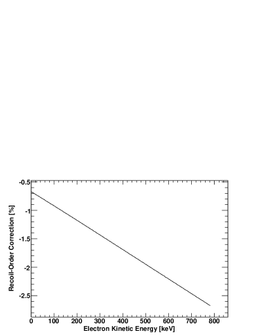
Figure 35: Energy dependence of the Standard Model recoil-order correction (calculated according to the formalism of wilkinson82 ; gardner01 ) for an extraction of $A_{0}$ from the measured asymmetry $A_{3}$.

Monte Carlo calculations of the $\Delta_{2,i}$ and $\Delta_{3}$ correction factors were carried out for each of the Geometries, thus accounting for their different foil thicknesses, their different measured MWPC efficiencies (recall the discussion of such in Section V.13), and their different two-fold PMT trigger threshold functions (Section V.11). To account for the previously-discussed (Section VI.4.2) known deficit in the GEANT4 backscattering strengths, backscattering events in the Monte Carlo were re-weighted, with a scaling factor of $f_{\text{bulk}}$ applied to Type 1 and Type 3 events, and $f_{\text{thin}}$ applied to Type 2 events and those events misidentified as Type 0 events (i.e., the “missed” backscattering events discussed in Section V.1). However, note that the $\Delta_{3}$ correction factors were evaluated in Monte Carlo without the $f_{\text{bulk}}$ and $f_{\text{thin}}$ re-weighting factors for the backscattering events. After application of the $\Delta_{2,i}$ backscattering corrections, the remaining $\Delta_{3}$ correction factor accounts for the distortion of the detected $\langle\beta_{\text{recon}}\cos\theta\rangle$ acceptance from the “true” $\langle\frac{1}{2}\beta_{\text{true}}\rangle$ distribution. Therefore, employing these $f_{\text{bulk}}$ and $f_{\text{thin}}$ re-weighting factors for the evaluation of the $\Delta_{3}$ correction factor in Monte Carlo would have biased the angular distribution of the simulated events, as the probablity for backscattering increases with angle.

The results of these calculations are plotted in Figs. 33 and 34 as a function of $E_{\text{recon}}$ for each of the Geometries. Figure 33 shows the calculated results for the $\Delta_{2}$ and $\Delta_{3}$ corrections, and the size of their combined correction, $(1+\Delta_{2})(1+\Delta_{3})$. For completeness, Fig. 34 then shows the sources of the individual $\Delta_{2,i}$ contributions to $\Delta_{2}$. All of the corrections shown here were calculated for the default Analysis Choice 3. The systematic uncertainties in these calculations are discussed in detail later in Section VIII.12. Note that the results for $\Delta_{2}$ and $\Delta_{3}$ are shown over an $E_{\text{recon}}$ energy range of 150–750 keV. Below 150 keV, the corrections become quite large, as the acceptance is highly suppressed for large pitch angle events and the probability for backscattering increases with decreasing energy.

Our sign convention for these corrections is such that if the correction factor $\Delta_{j}>0$, the resulting asymmetry calculated according to $A_{i}(1+\Delta_{j})$ is larger in magnitude (i.e., a more negative value for the asymmetry). As can be seen in Fig. 33, the $\Delta_{2}$ correction factors are $>0$ for all energies and Geometries, whereas the $\Delta_{3}$ correction factors are $<0$. The conceptual physical explanation for this is as follows.

With regard to a physical explanation for $\Delta_{2}$, the $\Delta_{2,i}$ correction factors correct the measured asymmetries for events misidentified in data analysis as a Type $i$ event. For example, an electron incident initially on one of the detectors could backscatter from either the decay-trap end-cap foil or the MWPC entrance window and then be detected in the opposite side’s MWPC and scintillator (e.g., the “Missed” event illustrated in Fig. 7); however, such an event would subsequently be misidentified in data analysis as a Type 0 event (with an incorrect initial direction). Because this type of event would dilute the magnitude of the measured asymmetry for Type 0 events, the Monte-Carlo-calculated $\Delta_{2,0}$ correction factor would be $>0$ (i.e., so as to increase the magnitude of the asymmetry, per our sign convention) to compensate for the dilution. Further, as the probability for backscattering from plastic scintillator decreases with energy over the energy range of neutron $\beta$-decay martin06 (and also for backscattering from thin Mylar films, as calculated in GEANT4 and verified via analytic integration of the differential cross section for the Mott scattering of electrons from atomic electrons), the $\Delta_{2,0}$ correction factor decreases with energy. Thus, conceptually, the $\Delta_{2,i}$ correction factors are expected to be $>0$ for all energies and to decrease in magnitude with energy, which is consistent with the results from our Monte Carlo calculations shown in Fig. 33.

With regard to a physical explanation for $\Delta_{3}$, there are two potential sources of bias to the $\langle\beta\cos\theta\rangle$ acceptance. First, there is a bias to the $\langle\cos\theta\rangle$ value, as the acceptance for large pitch angles is suppressed (e.g., from “Lost” events such as those shown in Fig. 7), with the value of $\langle\cos\theta\rangle>1/2$ for detected events (as the acceptance is biased towards small pitch angle events). Thus, in general, $\Delta_{3}$ is expected conceptually to be negative, given our definition of $(1+\Delta_{3})=\langle\frac{1}{2}\beta_{\text{recon}}\rangle/\langle\beta_{\text{true}}\cos\theta\rangle$ in Eq. (31). Second, because the energy loss in the decay-trap end-cap foils and the MWPC windows is strongly angle-dependent, the $E_{\text{vis}}$ visible energies in each visible energy bin, which then map to $E_{\text{recon}}$ values via the (mostly linear) parametrizations discussed in Section V.14, actually correspond to a distribution of initial true energies. Therefore, there is a bias to the assumption that the value of $\langle\beta_{\text{true}}\rangle=\langle\beta_{\text{recon}}\rangle$ in each $E_{\text{recon}}$ bin, which is corrected for in our Monte Carlo calculations of $\Delta_{3}$. The variation of $\Delta_{3}$ with energy depends on the details and shape of the initial energy distribution.

The differences between the values of the $\Delta_{2}$ and $\Delta_{3}$ correction factors for Geometry C and Geometry D (despite their identical foil thicknesses) is primarily because the measured MWPC thresholds for Geometry D were higher than those for Geometry C.

Finally, it is interesting to note that because $\Delta_{2}$ and $\Delta_{3}$ are of opposite signs, there is a “zero crossing” in the total correction factor $(1+\Delta_{2})(1+\Delta_{3})\approx 1+\Delta_{2}+\Delta_{3}$, which can be seen in Fig. 33.

As discussed in the upcoming Section VIII.12, the systematic uncertainties in these corrections were taken to be a relative fraction of the magnitude of these correction factors.

VII.6 Analysis Energy Window

Our final results for $A_{0}$ presented later in Section IX were obtained over an analysis energy window of 275–625 keV. This optimized energy window minimized the total absolute error in $A_{0}$ resulting from the quadrature sum of the statistical error and the energy-dependent systematic errors in the above-described Monte Carlo calculations of the $\Delta_{2}$ and $\Delta_{3}$ backscattering and angle effects corrections (which varied with energy as just shown in Figs. 33 and 34).

VII.7 Recoil-Order and Radiative Corrections

Table 8: Values of the $\Delta_{2}$ and $\Delta_{3}$ correction factors over the analysis energy window of 275–625 keV for each of the Geometries.

	Geometry A		Geometry B		Geometry C		Geometry D
$E_{\text{recon}}$ [keV]	$\Delta_{2}$ [%]	$\Delta_{3}$ [%]	$\Delta_{2}$ [%]	$\Delta_{3}$ [%]	$\Delta_{2}$ [%]	$\Delta_{3}$ [%]	$\Delta_{2}$ [%]	$\Delta_{3}$ [%]
275–300	2.28	$-1.17$	7.12	$-1.28$	1.57	$-0.43$	1.55	$-0.25$
300–325	1.89	$-1.58$	6.32	$-1.52$	1.36	$-0.49$	1.41	$-0.24$
325–350	1.63	$-1.38$	5.60	$-1.71$	1.30	$-0.40$	1.32	$-0.24$
350–375	1.54	$-1.43$	5.12	$-1.94$	1.18	$-0.28$	1.19	$-0.25$
375–400	1.33	$-1.45$	4.66	$-2.38$	1.04	$-0.50$	1.08	$-0.25$
400–425	1.25	$-1.67$	4.19	$-2.61$	1.05	$-0.43$	1.00	$-0.28$
425–450	1.16	$-1.66$	3.82	$-3.01$	0.91	$-0.53$	0.94	$-0.29$
450–475	1.04	$-1.96$	3.51	$-3.56$	0.89	$-0.76$	0.90	$-0.29$
475–500	1.04	$-1.91$	3.21	$-4.02$	0.87	$-0.63$	0.88	$-0.35$
500–525	0.97	$-2.16$	2.96	$-4.39$	0.85	$-0.63$	0.80	$-0.42$
525–550	0.92	$-2.51$	2.70	$-4.99$	0.77	$-1.00$	0.79	$-0.52$
550–575	0.85	$-2.44$	2.46	$-5.57$	0.83	$-1.10$	0.83	$-0.65$
575–600	0.84	$-3.03$	2.25	$-6.42$	0.73	$-1.20$	0.76	$-0.75$
600–625	0.84	$-3.02$	1.99	$-6.86$	0.70	$-1.13$	0.80	$-1.13$

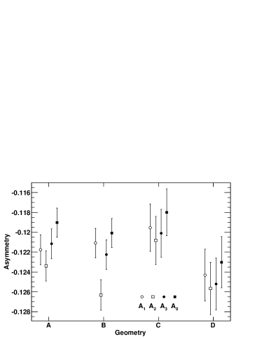
Figure 36: Results for the asymmetries $A_{1}$ (open circles), $A_{2}$ (open squares), $A_{3}$ (filled circles), and $A_{0}$ (filled squares) for each of the Geometries, integrated over the analysis energy window of 275–625 keV. All errors are statistical.

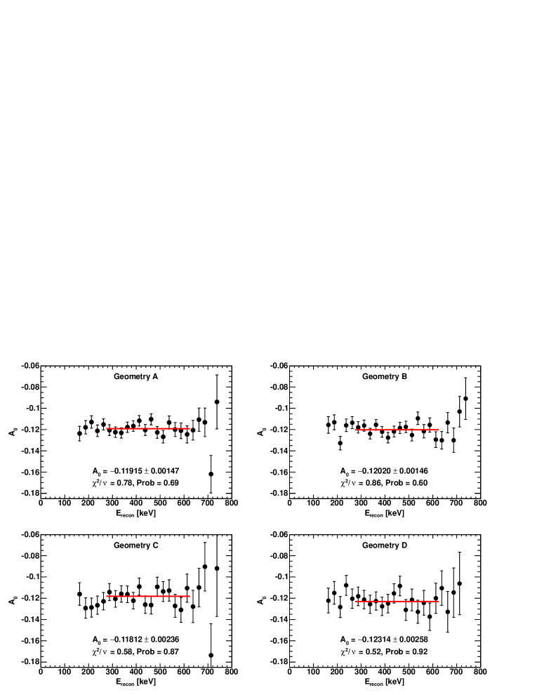
Figure 37: (Color online) Geometry-by-Geometry results for $A_{0}$ values extracted bin-by-bin. The solid red lines indicate the analysis energy window of 275–625 keV. The quoted errors are statistical.

Recoil-order corrections to the asymmetry were calculated within the context of the Standard Model according to the formalism of wilkinson82 ; gardner01 . The numerical results from these two parametrizations agree to better than $2\times 10^{-5}$. These parametrizations for the asymmetry $A$, Eq. (6), were then folded over the $\beta$-decay energy spectrum (including contributions from the Fermi function). In general, these recoil-order corrections increase the magnitude of the measured asymmetry over that of $A_{0}$; thus, an extraction of $A_{0}$ from the measured asymmetry requires (per our sign convention) a negative correction (i.e., a decrease in the magnitude of the asymmetry). The energy-dependence of this correction is shown in Fig. 35. For our analysis energy window of 275–625 keV, the integrated recoil-order correction (assuming the Particle Data Group average value for $\lambda$) was $(-1.79\pm 0.03)$% to $A_{0}$, where the $\pm 0.03$% uncertainty corresponds to the Particle Data Group’s statistical uncertainty in $\lambda$.

The value for the radiative correction was taken from the calculations of gluck92 , who presented results for the absolute (as opposed to relative) value of the radiative correction to the asymmetry. These calculations were performed using the average value for $\lambda$ available at that time, and were reported at six discrete values of electron energy. In general, these radiative corrections increase the magnitude of the measured asymmetry by $\sim 0.1$% over the range of our 275–625 keV analysis energy window. However, at the time of this analysis, we were not aware of the functional form for the energy-dependence of these radiative corrections which is presented in shann71 . Therefore, we applied a $(0.10\pm 0.05)$% correction to our asymmetries (again, per our sign convention), where our estimated $\pm 0.05$% uncertainity accounts for differences between the value of $\lambda$ available at the time of the calculation (1992, gluck92 ) and its present value, and for our incomplete knowledge at the time of the energy-dependence for the radiative correction.

Per the discussion in czarnecki04 , application of this radiative correction to our reported value for $A_{0}$ then permits extraction of a value for $g_{A}$ which can be compared with the expression relating $G_{F}$, $\tau_{n}$, $g_{A}$, and $V_{ud}$, Eq. (3), in which the (1 + RC) electroweak radiative corrections have been factorized in the same way for both the vector and axial-vector interactions czarnecki04 .

VII.8 Comparison of Geometry-by-Geometry Results

The values for the $\Delta_{2}$ and $\Delta_{3}$ corrections in Geometry over our analysis energy window of 275–625 keV are tabulated in Table 8 for all of the Geometries. Figure 36 then compares the resulting Geometry-by-Geometry asymmetries $A_{1}$, $A_{2}$, $A_{3}$, and $A_{0}$ integrated over the analysis energy window. The final values for $A_{0}$ from each of the Geometries are all seen to be statistically consistent. Geometry-by-Geometry results for the $A_{0}$ values extracted bin-by-bin are shown in Fig. 37.

We emphasize that the agreement between our results from the different Geometries provides confidence in our Monte Carlo treatment of the backscattering and $\langle\beta\cos\theta\rangle$ acceptance effects. In particular, the result from Geometry B (thickest decay trap end-cap and MWPC foils) agrees well with those from the other Geometries, in spite of its relatively larger $\Delta_{2}$ and $\Delta_{3}$ corrections (compare the differences in $A_{1}$, $A_{2}$, and $A_{3}$ for Geometry B with those for the other Geometries).

Table 9: Background-subtracted neutron $\beta$-decay rates integrated over the complete energy range of 0–800 keV after all analysis cuts.

		East Detector	West Detector
Geometry	Spin State	Rate [s-1]	Rate [s-1]
A	$-$	4.79	4.90
A	$+$	3.82	3.25
B	$-$	6.50	6.87
B	$+$	5.43	4.78
C	$-$	3.29	3.42
C	$+$	2.81	2.44
D	$-$	6.45	6.61
D	$+$	4.80	4.12

Finally, for completeness, our background-subtracted neutron $\beta$-decay rates integrated over the complete energy range of 0–800 keV after all analysis cuts are listed in Table 9 for all the Geometries and for both spin states. As previously discussed in Section V.4, the data quality analysis cuts related to DAQ electronics problems removed a significant fraction of the Geometry A and Geometry B events (up to $\sim 30$%). Another significant analysis cut included the 45 mm radius fiducial cut discussed in Section V.6.2, which removed $\sim 25$% of the events. Finally, under the 275–625 keV analysis energy window, the rates from 0–800 keV listed in Table 9 would be reduced by another factor of $\sim 40$%.

VIII Systematic Uncertainties

VIII.1 Summary

Table 10: Summary of systematic corrections and uncertainties. All numbers quoted are fractional [%] relative to $A_{0}$. Upper Table: Geometry-Independent systematic uncertainties. No systematic corrections were applied for these effects (with the exception of the radiative corrections, already discussed in Section VII.7). Lower Table: Geometry-Dependent systematic corrections and uncertainties. The quoted value denotes the systematic correction, with the error the systematic uncertainty. As discussed in the text, $\Delta_{2}$ represents the correction for backscattering, and $\Delta_{3}$ the correction for the angle effect. $\epsilon_{\text{MWPC}}$ denotes the systematic uncertainty associated with the MWPC efficiency.

Geometry-Independent Effect	Uncertainty [%]
Dead Time	$\pm 0.01$
Energy Reconstruction	$\pm 0.47$
Fiducial Cut and Coordinate Systems	$\pm 0.24$
Gain Fluctuations	$\pm 0.20$
Live Time	$\pm 0.24$
Magnetic Field Nonuniformity	${}^{+0.20}_{-0.00}$
Muon Veto Efficiency	$\pm 0.30$
Neutron-Generated Backgrounds	$\pm 0.02$
Polarization	${}^{+0.52}_{-0.00}$
Radiative Corrections	$\pm 0.05$
Rate-Dependent Gain Shifts	$\pm 0.08$

Geometry-Dependent Effects
	A [%]	B [%]	C [%]	D [%]
$\Delta_{2}$	$1.34\pm 0.40$	$4.32\pm 1.30$	$1.07\pm 0.32$	$1.08\pm 0.32$
$\Delta_{3}$	$-1.81\pm 0.45$	$-3.22\pm 0.81$	$-0.60\pm 0.15$	$-0.36\pm 0.09$
$\epsilon_{\text{MWPC}}$	$0.00\pm 0.02$	$0.00\pm 0.01$	$0.00\pm 0.16$	$0.00\pm 0.50$

Our systematic corrections and uncertainties are summarized in Table 10, where we have categorized the effects as either Geometry-Dependent (i.e., effects which varied with the decay trap end-cap foil and MWPC window thicknesses, measured detector thresholds, etc.), or Geometry-Independent (e.g., UCN polarization, dead time effects, etc.) In the rest of this Section we discuss each of these systematic effects (in the order in which they appear in Table 10) in more detail.

VIII.2 Geometry-Independent: Dead Time

Nearly all dead time effects cancel in the super-ratio technique. Indeed, in order for there to be any bias to the asymmetry resulting from dead time effects in the background-subtracted $\beta$-decay rates, there must be a difference in the two detectors’ dead times, and there must be a difference in a particular detector’s dead time for the two neutron spin states. Thus, these effects are expected to be quite small.

Nevertheless, as previously noted in Section III.8, the dead time of the DAQ system was monitored by counting, in scalers, the total number of detector two-fold PMT triggers, including those that were vetoed by the DAQ “busy logic” during the $\sim 12$ $\mu$s readout gates for the PADC modules. However, to avoid spurious (and correlated) trigger chains from scintillator afterpulses (as noted earlier in Section III.8) distorting the determination of the dead time, the dead time was determined only from the scaler counts of detector triggers that occurred during triggers from the opposite-side detector or from other experimental triggers, such as the UCN monitors. The dead time, as extracted from the correlation between the DAQ trigger rate and the fraction of these “missed triggers”, was found to be $\sim 13.5$ $\mu$s, which is consistent with the nominal $\sim 12$ $\mu$s system dead time (associated with the gate for the PADC readout). Further, the difference in the fraction of “missed triggers” for (up to) a 20 s^-1 trigger rate difference between the two spin states is no larger than $\sim 0.03$%. Considered together, any possible bias to the asymmetry was no greater than 0.01%, which is the error we quote in Table 10.

Alternatively, another possible way dead time effects could bias the asymmetry is in the background subtraction procedure, resulting from differences in the DAQ total trigger rates during $\beta$-decay and background runs. However, these effects tend to cancel in the super-ratio, as the four background-subtracted $\beta$-decay rates appearing in the super-ratio would be expected to be biased in the same direction. Further, the effect is minimized as the signal-to-background ratio increases. Under the conservative assumption of a 200 s^-1 DAQ trigger rate difference (e.g., from differences in the scintillator trigger rates, UCN monitor trigger rates, etc.) for $\beta$-decay versus background runs, and a signal-to-background ratio greater than 5, any such systematic bias to the asymmetry from dead time effects is $\ll 0.01$%.

VIII.3 Geometry-Independent: Energy Reconstruction

Figure 17 showed the error envelope for the uncertainty in the visible energy calibration. To estimate the systematic error associated with possible errors in our energy calibration, we generated a large number (200 per Geometry) of random error curves that were constrained to fit within the limits of this error envelope. We then extracted from these error curves their contributions to an error in the asymmetry, resulting from an incorrect reconstruction of the electron energy, and hence $\langle\beta\cos\theta\rangle$. From these calculations we concluded that the maximum (i.e., worst case) error, resulting from the case where the error curves for the two detectors are identical, is a fractional 0.47% uncertainty in the asymmetry for the analysis energy window of 275–625 keV. As a conservative estimate of the systematic uncertainty associated with our energy calibration, we then assign this worst-case error of 0.47% to be the systematic uncertainty associated with possible errors in our energy calibration.

As discussed earlier in Section V.14, the default $E_{\text{recon}}$ parametrization we employed was based on a fit to the scintillator visible energy $E_{\text{vis}}$ only; by constrast, an alternative $E_{\text{recon}}$ fit included both $E_{\text{vis}}$ and the calibrated MWPC energy $E_{\text{MWPC}}$. To study the sensitivity of the reconstructed asymmetry to these two different $E_{\text{recon}}$ parametrizations, we extracted values for the energy-corrected asymmetry $A_{1}$ for these two different fits. The difference between these two methods, averaged over the entire data set, was 0.2%. This is small relative to the 0.47% systematic uncertainty associated with the energy calibration, and we also noted in Section V.14 that this alternative $E_{\text{recon}}$ parametrization based on both $E_{\text{vis}}$ and $E_{\text{MWPC}}$ is subject to (uncorrectable) overflow of the MWPC anode readout.

Another source of a systematic error resulting from the energy reconstruction as discussed in detail in Section VI.5 (and shown in Fig. 29) was the observed systematic $\sim 10$–14 keV difference between the fitted endpoints and the Monte Carlo prediction. We investigated the systematic uncertainty to the extracted asymmetry due to this systematic difference by extracting a “stretching factor”, $f\equiv T_{0,\text{MC}}/T_{0,\text{fit}}$, where $T_{0,\text{MC}}$ denotes the Monte Carlo predicted endpoint and $T_{0,\text{meas}}$ the fitted endpoint, for each run. The data were then re-analyzed by applying on an event-by-event basis this “stretching factor” to the reconstructed energy $E_{\text{recon}}$, thus effectively forcing the fitted endpoints to match the Monte Carlo predicted endpoints. The asymmetries extracted from the “streched” data differed by $<0.07$% from the (original) “unstretched” data which, again, is much less than the 0.47% error associated with the energy calibration.

Finally, to account for a slight mismatch ($\sim 2$ keV) between the Monte Carlo and measured energy spectra (this is visible in the final $E_{\text{recon}}$ spectrum later in Fig. 40) we fitted the Monte Carlo visible energy spectra to the measured visible energy spectra, and then extracted values for the asymmetry assuming these modified values for the visible energy. The bias to the asymmetry was $0.13$% averaged over all four Geometries which, again, is much less than the 0.47% the energy calibration uncertainty.

VIII.4 Geometry-Independent: Fiducial Cut and Coordinate Systems

As discussed in Section V.6.2, we required backscattering events to satisfy a default vertex cut of $|\vec{x}_{E}-\vec{x}_{W}|<25$ mm. We studied the impact of this cut on the asymmetry by varying this cut from 10 mm to 40 mm; the effect on the asymmetry was $<0.1$%, indicating a negligible systematic effect.

As was also discussed there, our fiducial cut required the position (radius) of the event on the primary triggering scintillator side to satisfy $r_{\text{trigger}}<45$ mm. To examine whether there was any position bias, we extracted the asymmetry in successive annuli via cuts on $r^{2}$ in six different annular bins, ranging from [0,400] mm² to [2025,2500] mm². The asymmetries in all of these annuli were in statistical agreement, with no statistical evidence for any systematic difference with position.

Recall also in Section V.6.2 we noted the possibility for the definition of four different coordinate systems. To determine whether there was any bias resulting from the choice of the coordinate system (for example, a consideration could be whether there were any systematic variations in the backscattering fractions in the vicinity of the fiducial cut), we studied the variation of the asymmetry with the choice of coordinate system, and for fiducial volume radius cuts of 45 mm and 50 mm. The RMS spread in the asymmetries for the different coordinate system choices was 0.24% for the 45 mm radius cut and 0.21% for the 50 mm radius cut. Although the RMS spread for the 50 mm radius cut was actually somewhat smaller (suggesting that employing a larger fiducial volume would have introduced no bias to the asymmetry), we nevertheless chose the 45 mm radius cut as our (conservative) definition of the fiducial volume, and thus assigned a 0.24% systematic uncertainty to the definition of the fiducial volume.

VIII.5 Geometry-Independent: Gain Fluctuations

As noted in Section III.6, the PMT gains were monitored on a run-to-run basis using the minimium-ionizing peak from cosmic-ray muon events. Nevertheless, any residual uncompensated run-to-run gain fluctuations could bias the asymmetry on a run-to-run basis; however, any such short-term run-to-run fluctuations will average away according to the usual $1/\sqrt{N_{\text{run}}}$ statistics assuming the long-term gain corrections are accurate. We estimated the level of any such run-to-run residual gain errors by extracting the level of fluctuations in the run-to-run fitted values for the $\beta$-decay spectrum endpoint. These were typically of order $\sim\pm 1.2$% in each detector, with the gain fluctuations in the two detectors only slightly correlated relative to each other. [Correlated gain fluctuations are significantly more problematic than are anti-correlated gain fluctuations.] Conservatively assuming the worst-case sensitivity for gain fluctuations in one of the Geometries to be representative of the entire data set, we quote a systematic uncertainty of 0.20% for uncompensated gain fluctuations.

VIII.6 Geometry-Independent: Live Time

The detector rates (and, hence, asymmetries) were ultimately calculated from the number of events passing the analysis cuts normalized to the detectors’ respective live times; the concept of the detector live time was discussed in detail previously in Section V.4. As discussed there, we defined a run’s live time to be the fraction of that run surviving all of the global data quality cuts. However, as we noted there, it was necessary to apply a correction for the Geometry B live times due to the large fraction (up to $\sim 30$%) of events suffering from an event-by-event TDC event counter problem. The correction factors for each run were determined using events identified as gamma rays, which were statistically independent of the neutron $\beta$-decay events and also provided higher statistics (event rates up to 100 s^-1 in each detector) than the neutron $\beta$-decay events themselves for the calculation of the correction factors. The resulting correction factors, defined to be the ratio of the number of gamma ray events surviving the event-by-event TDC event counter cut to the total number of gamma ray events, were then computed on a run-by-run basis for each detector.

Only the Geometry B live times were corrected according to this procedure. Nevertheless, to assess the systematic error associated with our definition of and calculation of the live time, we extracted values for the asymmetries for all four Geometries with and without application of these live time correction factors (the correction factors for Geometries A, C, and D were small, with the values for the asymmetries differing by $<0.1$% under the two scenarios). Averaged over all four Geometries, the difference between the asymmetries extracted under these two different scenarios was 0.24%, which is the value for the systematic uncertainty associated with this effect we quote in Table 10.

VIII.7 Geometry-Independent: Magnetic Field Nonuniformity

Our Monte Carlo calculations of the corrections for backscattering and the $\langle\beta\cos\theta\rangle$ acceptance discussed in Section VII.4 assumed a uniform magnetic field in the decay trap region. We studied the impact of the actual measured nonuniformity in the spectrometer magnetic field shown previously in Fig. 4 in Monte Carlo. Qualitatively, the impact of the $\sim 30$ Gauss “field dip” in the central decay-trap region is such that electrons from decays occuring in this “field dip” region are either reflected (analogous to backscattering) or are trapped (for large pitch angles). We studied these effects in our GEANT4 Monte Carlo simulation program by implementing the magnetic field profile shown in Fig. 4 directly in the simulation. Neutron $\beta$-decay events were then generated uniformly along the length of the decay trap.

In the Monte Carlo, $\sim 0.3$% of the events incident initially on one of the two detectors were reflected from the field dip, with an average $\langle\beta\cos\theta\rangle$ of $\sim 0.02$. Because this small fraction of events carries little $\langle\beta\cos\theta\rangle$ “analyzing power”, the resulting bias to the asymmetry is negligible. The fraction of electrons trapped by the field dip was $\sim 2.6$%, again with an average $\langle\beta\cos\theta\rangle$ of $\sim 0.02$. The remaining 97.1% of the events were not impacted by the field dip. Assuming that the electrons trapped by the field dip eventually scatter from residual gas molecules, the impact is a dilution to the asymmetry. The calculated dilution to the asymmetry was $-0.2$%. In lieu of applying a correction to the asymmetry, we assigned a ${}^{+0.2\%}_{-0.0\%}$ systematic uncertainty to this effect. We also note that our Monte Carlo calculations found that the time for a trapped electron to scatter from residual gas for a vacuum pressure of $10^{-5}$ Torr is $\sim 4$ ms, with a small distortion to their energy distribution of $\sim-8$ keV.

Note that our Monte Carlo results for the fraction of events trapped by the field dip and their average value of $\langle\beta\cos\theta\rangle$ are consistent with the following simple estimates. As discussed earlier in Section III.5.1, electrons emitted with some momentum $p_{0}=(p_{\perp,0}^{2}+p_{\parallel,0}^{2})^{1/2}$, with $p_{\perp,0}$ ($p_{\parallel,0}$) the initial transverse (longitudinal) momentum component, in some local field $B_{0}$ will be reflected from higher field regions $B$ if $B>B_{\text{crit}}\equiv(p_{0}^{2}/p_{\perp,0}^{2})B_{0}$ (thus, only the pitch angle $\theta$ of the emitted electron is relevant, not the magnitude of the momentum). Taking $B_{0}=0.9925$ T and $B=0.9955$ T for the measured 2009 field profile (here, $B$ is taken to be the average of the local maxima at $z=-100$ cm and $+50$ cm) shown in Fig. 4, one finds electrons with pitch angles $\theta>\theta_{\text{crit}}=86.9^{\circ}$ will be trapped in the field dip region.

Approximating the initial angular distribution of emitted electrons as isotropic (reasonable, given that the $\beta$-asymmetry is an $\mathcal{O}(10\%)$ effect), one finds that the fraction of electrons emitted in the local field dip region $B_{0}=0.9925$ T which will be trapped is

$$f_{\text{trap}} = \frac{1}{4\pi}2\times{\int_{\theta_{\text{crit}}}^{\pi/2}}\sin\theta d\theta{\int_{0}^{2\pi}d\phi}=\cos\theta_{\text{crit}}$$ (34)

$$= 0.054.$$

Then, assuming a uniform distribution of events along the 300-cm long decay trap, the fraction of events emitted in the $\sim 150$-cm long field dip region is $\sim 0.5$, implying the total fraction of events generated over the length of the decay trap which will be trapped in the field dip region is $\sim 0.027$, which is consistent with the Monte Carlo result of 2.6%. For a nominal value of $\beta\sim 0.75$, $\langle\beta\cos\theta\rangle\approx\beta\cos[(\theta_{\text{crit}}+\pi/2)/2]=0.02$ for these trapped events, again, consistent with the Monte Carlo result.

VIII.8 Geometry-Independent: Muon Veto Efficiency

We estimated the effect of a possible systematic uncertainty resulting from fluctuations in the muon-veto efficiency by extracting values for the asymmetries with and without application of the muon-veto detector cuts. Averaged over Geometries, the variations in the asymmetry were at the 0.3% level.

We note that the assignment of this 0.3% uncertainty is quite conservative. A linear drift in the muon veto cut efficiency would be equivalent to a linear drift in the backgrounds, and as discussed in Section VI.3, linear background drifts cancel under the octet-based super-ratio asymmetry structure.

VIII.9 Geometry-Independent: Neutron-Generated Backgrounds

As already dicussed in detail, ambient backgrounds were measured and subtracted on a run-by-run basis. However, a possible source of irreducible backgrounds was neutron capture on materials near the electron detectors, generating prompt gamma rays with energies up to 7.9 MeV, 7.1 MeV, 6.8 MeV, 4.9 MeV, or 8.2 MeV for capture on ⁶³Cu, ⁶⁵Cu, ⁹Be, ¹²C, or ¹³C, respectively, the elements of which the decay trap and end-cap foils were primarily composed. Such backgrounds cannot, of course, be subtracted.

This background was expected to be significantly suppressed in the UCNA experiment as compared to previous cold neutron beam experiments because, as discussed earlier in Section III.1, the fraction of neutrons present in the apparatus which contribute to the decay rate is orders of magnitude larger in the UCNA Experiment than in previous cold neutron beam experiments, and also because of the small probability for capture and upscatter by UCN stored in the decay trap.

We carried out three different approaches to our assessment of the contamination level from any such backgrounds. The idea of our first approach is as follows. If a gamma ray emitted from a neutron capture subsequently interacted with the scintillator, the MWPC should not have recorded any energy deposition if the gamma ray forward Compton scattered in the scintillator. Further, as calculated in simulations, there is a factor of 10–20 suppression in the fraction of gamma ray events incident on the electron detectors triggering both the scintillator and MWPC as compared to those triggering only the scintillator. Therefore, any such neutron-generated backgrounds should appear as non-zero residuals in a comparison of background-subtracted scintillator spectra [i.e., ($\beta$-decay run $-$ background run) spectra] formed with and without application of a MWPC-scintillator coincidence cut. In particular, an excess would be expected in the background-subtracted spectrum constructed without the requirement of a MWPC-scintillator coincidence cut as compared to the background-subtracted spectrum obtained with the requirement of a MWPC-scintillator coincidence cut.

Now consider the following model. Under application of a MWPC coincidence cut, let

$$R_{\text{cut}}=\epsilon\left(S_{\text{cut}}-B_{\text{cut}}\right),$$ (35)

where $R_{\text{cut}}$ denotes the resulting background-subtracted scintillator event rate, $S_{\text{cut}}$ and $B_{\text{cut}}$ denote, respectively, the underlying $\beta$-decay + background and background event rates, respectively, and $\epsilon$ denotes the MWPC cut efficiency. We then write a similar expression for the background-subtracted scintillator event rates obtained without application of a MWPC cut as

$$R_{\text{no cut}}=\left(S_{\text{cut}}-B_{\text{cut}}\right)+\left(S_{\gamma}-B_{\gamma}\right),$$ (36)

where now $S_{\gamma}$ and $B_{\gamma}$ denote the signal and background rates during the $\beta$-decay and background runs from gamma ray events which would otherwise fail the MWPC cut. Note that in the absence of any neutron-generated gamma rays, the statistical averages of $S_{\gamma}$ and $B_{\gamma}$ should be identical.

The difference between $R_{\text{no cut}}$ and $R_{\text{cut}}$ is then

$$\Delta R = R_{\text{no cut}}-R_{\text{cut}}$$ (37)

$$= \left(S_{\gamma}-B_{\gamma}\right)+\left(S_{\text{cut}}-B_{\text{cut}}\right)(1-\epsilon)$$

$$= \Gamma_{\gamma}+(1-\epsilon)\Gamma_{n},$$

where $\Gamma_{\gamma}$ and $\Gamma_{n}$ denote, for gamma ray and neutron $\beta$-decay events, respectively, the difference between the background-subtracted scintillator rates with and without application of a MWPC coincidence cut. Thus, this model then requires an estimate for the MWPC cut efficiency.

We extracted a value for our MWPC cut efficiency by examining the MWPC anode spectrum for ¹¹³Sn source calibration data. After placing a FWHM cut on the scintillator visible energy spectrum, we then fitted the resulting MWPC spectrum (such as shown, for example, in Fig. 10) to a Landau distribution, and its pedestal to a Gaussian. We then calculated the fraction of the Landau distribution falling below the cut line, which should provide an estimate of the MWPC cut efficiency. These values were found to be 99.93(3)% and 99.95(3)% for the East and West detector, respectively. We do note that this provides for an estimate of the MWPC efficiency only at the ¹¹³Sn energy.

The residual $\Delta R$ (no MWPC cut $-$ MWPC cut) rates integrated over the analysis energy window (and after all analysis cuts) ranged from $1.0\times 10^{-3}$ s^-1 to $6\times 10^{-3}$ s^-1 for the two detectors and two spin states for all four Geometries, representing $\sim 10^{-3}$ of the $\beta$-decay rates. After accounting for the factor of 10–20 supression for the fraction of events which would trigger both the scintillator and MWPC, the estimated contamination fractions for the actual $\beta$-decay analysis employing the MWPC-scintillator coincidence cut are then on the order of $10^{-4}$. Propagation of the measured contamination fractions (for each detector and spin state) through the super ratio then led to a systematic bias to the asymmetry of order $\sim 0.02$%.

In our second approach, we extrapolated the residual background (i.e., after background subtraction) above the $\beta$-decay endpoint into the signal region. Above the endpoint, the residual background-subtracted rates in the 25 keV $E_{\text{recon}}$ bins were typically of order $10^{-4}$ s^-1 or less. Under the assumption that the neutron-generated background is independent of energy (e.g., as was employed in the analysis of abele02 ), we then extrapolated these above-the-endpoint rates into the analysis energy window. The resulting contamination fractions, $\sim 10^{-4}$–$10^{-3}$, were similar to the analysis in our first approach comparing background-subtracted scintillator spectra obtained with and without a MWPC cut. These contamination fractions were again propagated through our super-ratio asymmetry analysis, and the systematic bias was again found to be of order $\sim 0.02$%.

Finally, in our third approach, we carried out a “beta-blocker” measurement in which a 6.35-mm thick piece of acrylic was placed between the decay trap and the MWPC in the field-expansion region of the spectrometer, as indicated schematically in Fig. 38. The idea for this measurement was two-fold: (1) the acrylic was sufficiently thick to stop the endpoint $\beta$-decay electrons, thereby “blocking” the $\beta$-decay signal of interest; and (2) the acrylic then served as a “source” of Compton-scattered electrons, resulting from interactions of neutron-generated gamma rays with the acrylic.

Measurements were conducted with this piece of acrylic at two different positions, A and B, as shown in Fig. 38, in front of one of the detectors. The motivation for doing so was that a comparison of the results from positions A and B should, in principle, permit a decomposition of the measured detector signal into contributions from Compton-scattered electrons originating in this acrylic piece (the solid angle for which was clearly smaller in position B as compared to position A), and direct neutron-generated gamma-ray interactions in the plastic scintillator detector (which should not have varied with the position of the acrylic piece).

Figure 38: Schematic diagram of the “beta-blocker” measurement of neutron-generated backgrounds. The dashed lines are meant to indicate the solid angle for production of Compton-scattered electrons in the acrylic at the two different positions.

Note that this measurement is subject to some model dependence, including an assumption for the source positions along the decay trap of the neutron-generated backgrounds (which determines the ratio of the solid angles for positions A and B). Our resulting estimates for the contamination fraction, as extracted from our measurements of the residual (background-subtracted) rates with the acrylic piece located at both positions A and B (under the assumption that the ratio of the A and B solid angles for production of Compton-scattered electrons was 20:1), were of order $10^{-3}$. Then accounting for the factor of 10–20 suppression for gamma ray events triggering both the scintillator and MWPC (in the actual geometry) leads to an estimate for the contamination fraction on the order of $10^{-4}$, consistent with the other two approaches.

VIII.10 Geometry-Independent: Polarization

The UCN polarization systematic was discussed earlier in Section IV.3. Because the measured depolarization was consistent with zero at the $1\sigma$ level (i.e., $P>0.9948$), we did not apply a correction for the polarization, and instead quote a one-sided systematic uncertainty in $A_{0}$ of ${}^{+0.52\%}_{-0.00\%}$ resulting from the constraint $P>0.9948$.

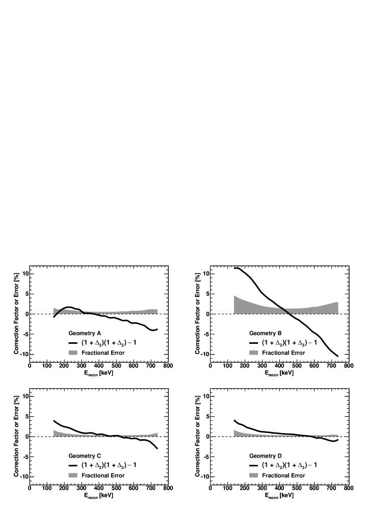
Figure 39: Results from GEANT4 Monte Carlo calculations of the relative size of the combined $\Delta_{2}$ backscattering and $\Delta_{3}$ angle effect fractional systematic correction (thick solid lines) and the total fractional systematic uncertainty assigned to these corrections (gray bands).

VIII.11 Geometry-Independent: Rate-Dependent Gain Shifts

A potential systematic effect would arise from any spin-state-correlated systematic gain shifts, such as from rate-dependent gain shifts. However, any such gain shifts shared by both detectors cancel to first order in the super ratio asymmetry and are thus expected to be small. As noted earlier in Section III.2, during the operation of the experiment, the total DAQ recorded data rates (i.e., the “online” $\beta$-decay rates integrated over all energies with few cuts) during $\beta$-decay runs for the non-flipped spin state were typically $\sim 10$ s^-1 greater than those recorded during measurements of the flipped spin state. By taking data with calibration sources with different activities, we were able to bound any such rate-dependent gain shifts to then be $<0.02$%/($\sim 10$ s^-1), which corresponds to a systematic uncertainty in the asymmetry of $\lesssim 0.08$%.

VIII.12 Geometry-Dependent: Backscattering $\bm{\Delta_{2}}$ and Angle Effect $\bm{\Delta_{3}}$ Corrections

Our working assumption was that application of the $f_{\text{bulk}}$ and $f_{\text{thin}}$ scale factors to the GEANT4 backscattering distributions calibrated our Monte Carlo calculations of our $\Delta_{2}$ backscattering corrections to the asymmetry. To estimate the uncertainty in these now-calibrated corrections, we compared the GEANT4 results for the $\Delta_{2}$ backscattering correction with the PENELOPE results. [Note that the PENELOPE calculations required $f_{\text{bulk}}$ and $f_{\text{thin}}$ scale factors of 0.9–1.1 and 1.3, respectively, somewhat smaller than those required by GEANT4.] These agreed to better than 22% for Geometry A, and better than 6% for Geometries B, C and D. We also note that the RMS of the $\Delta_{2}$ corrected asymmetries for Analysis Choices 1–5 was 0.10%, 0.13%, 0.30%, and 0.27% for Geometries A, B, C, and D, respectively, providing a powerful check of the robustness of the calculation of the $\Delta_{2}$ correction (indeed, consistent with the robustness of the agreement between the measured and simulated asymmetries for the various Analysis Choices demonstrated previously in Fig. 31). We have taken a conservative approach to our estimate of the systematic uncertainty in our backscattering corrections, and quote a 30% relative uncertainty in the $\Delta_{2}$ backscattering correction (and, thus, in the asymmetry) for all of the Geometries.

To estimate the systematic uncertainty in the $\Delta_{3}$ angle effect correction, we varied the thickness of the decay trap end-cap foil thicknesses in the Monte Carlo. Assuming 0.5 $\mu$m to be a reasonable uncertainty in the foil thickness, the relative uncertainty in $\Delta_{3}$ was found to be no larger than 25%. Further, we note that the GEANT4 and PENELOPE results for $\Delta_{3}$ agreed to better than $\sim 25$% for all of the Geometries. Therefore, we again quote a conservative 25% relative uncertainty in the $\Delta_{3}$ angle effects correction for all of the Geometries.

Figure 39 shows the resulting energy-dependent error bands for the combined $\Delta_{2}$ and $\Delta_{3}$ corrections for each of the Geometries. The analysis energy window of 275–625 keV referenced earlier in Section VII.6 was chosen such that the total error in $A_{0}$ resulting from integration of these error bands over some energy window combined with the statistical error within that energy window was a global minimum.

VIII.13 Geometry-Dependent: MWPC Efficiency

As discussed earlier in Section V.13, the “standard” MWPC cut for the separation of gamma rays and charged particles was a cut on a fixed PADC channel number. However, as shown there, the MWPC exhibited a strong position-dependent response. Therefore, for some particular energy deposition in the MWPC, employing such a standard cut resulted in a position-dependent efficiency for the identification of an event as either a gamma ray or charged particle event.

We investigated the impact of this position-dependent efficiency on the asymmetry by comparing results for the asymmetry extracted from analyses employing the standard PADC channel number cut with those obtained with fixed MWPC energy cuts ranging from 0.1–0.7 keV. The error bounds from this analysis appear as the MWPC efficiency systematic uncertainties in Table 10. Note that this effect is largest for Geometry D, for which the differences between the two MWPCs’ efficiency curves was greatest, as shown previously in Fig. 22.

IX Summary of Final Results

IX.1 Energy Spectra and Binned $\bm{A_{0}}$ Results

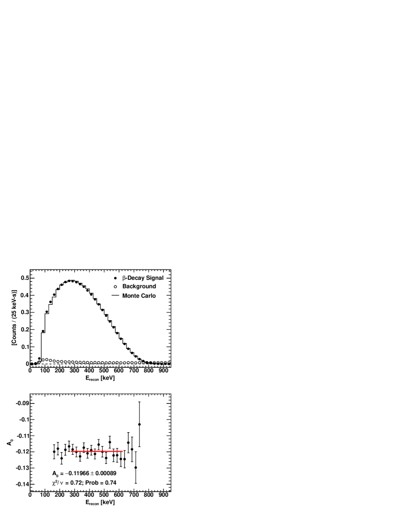
Figure 40: (Color online) Upper plot: Final results for the measured background $E_{\text{recon}}$ energy spectrum (open circles) and the background-subtracted neutron $\beta$-decay $E_{\text{recon}}$ energy spectrum (filled circles) summed over both detectors, averaged over the two neutron spin states, and then averaged over all four Geometries. The Monte Carlo prediction for the $E_{\text{recon}}$ spectrum is shown as the solid line. Lower plot: Final results for $A_{0}$ extracted bin-by-bin and then averaged over all four Geometries. The solid red line indicates the analysis energy window of 275–625 keV. The quoted error is statistical.

Our final results are shown in Fig. 40, where we compare the background-subtracted $\beta$-decay $E_{\text{recon}}$ spectrum, summed over both detectors, averaged over the two neutron spin states, and averaged over all four of the Geometries, with the Monte Carlo predicted $E_{\text{recon}}$ spectrum. There, we also show our Geometry-averaged energy-binned values for the $\beta$-asymmetry $A_{0}$, and the final statistical result of $A_{0}=-0.11966\pm 0.00089$. Note that the central value for $A_{0}$ was insensitive to the choice of analysis energy window, with the variation less than 15% of the statistical uncertainty for other windows between 150 and 750 keV.

IX.2 Final Combined Result

Each of the four Geometries yielded a data set with a statistical error and a systematic error. The statistical errors for each of these Geometries were, of course, independent. However, three of our dominant systematic uncertainties (energy reconstruction, backscattering, and angle effects) were all correlated. For example, a mistake in the decay trap end-cap window thickness would have biased the angle effects correction for all of the data sets. Therefore, we assume all three of these systematic uncertainties are 100% correlated across the four different Geometries.

Under this assumption, we then combined the results from the four Geometries according to the following procedure which incorporates correlations properly in the construction of a global $\chi^{2}$ stump01 . Each individual measurement $i$ gives a constraint of

$$A_{0}^{i}=A_{0}\pm\sigma_{i}+{\sum_{k=1}^{3}}\pm\sigma(\Delta_{k}^{i}),$$ (38)

where $A_{0}^{i}$ and $\sigma_{i}$ denote, respectively, the central value and statistical uncertainty for the $i^{\text{th}}$ measurement (i.e., Geometry), and the $\sigma(\Delta_{k}^{i})$ denotes the correlated uncertainty due to the three systematic effects just discussed. We then constructed a $\chi^{2}$ as

$$\chi^{2}={\sum_{i}}{\sum_{j}}(A_{0}^{i}-A_{0})(V^{-1})_{ij}(A_{0}^{j}-A_{0}),$$ (39)

where $i$ and $j$ are the indices of the measurements, and $V$ is the covariance matrix with $V_{ij}=\sigma_{i}^{2}\delta_{ij}+\sum_{k=1}^{3}\sigma(\Delta_{k}^{i})\sigma(\Delta_{k}^{j})$. As was shown in stump01 , the $\chi^{2}$ constructed this way satisfies a standard $\chi^{2}$ distribution, in which the value of $A_{0}$ follows from minimization of this $\chi^{2}$, and the one-sigma uncertainty is obtained from the usual condition $\chi^{2}-\chi^{2}_{\text{min}}=1$.

Using standard minimization techniques, the final combined result for $A_{0}$ we obtained is

$$A_{0} = -0.11966\pm 0.00089~{}_{-0.00140}^{+0.00123},$$

$$[\chi^{2}/\nu=2.4/3~{}(\text{Prob = 0.49})]$$

where the first (second) error represents the statistical (systematic) error. From this, we extract the following value for $\lambda=g_{A}/g_{V}$ under the Standard Model,

$$\lambda=\frac{g_{A}}{g_{V}}=-1.27590\pm 0.00239~{}_{-0.00377}^{+0.00331}.$$ (41)

X Summary and Conclusions

In this article we have presented a comprehensive and detailed description of the first precision result liu10 from the UCNA Experiment, an experiment designed to perform the first-ever measurement of the neutron $\beta$-asymmetry parameter $A_{0}$ with polarized ultracold neutrons. As demonstrated here, the use of UCN in a neutron $\beta$-asymmetry experiment controls key neutron-related systematic corrections and uncertainties, including the neutron polarization and neutron-generated backgrounds. Our result for the neutron polarization was shown to only be statistics limited, and our neutron-generated backgrounds were negligible to the level of $<0.1$% precision. All of our results reported here are consistent with our previously published proof-of-principle results obtained during data-taking runs in 2007 pattie09 .

Figure 41: (Color online) Ideogram of values for $g_{A}/g_{V}$ extracted from measurements of the neutron $\beta$-asymmetry parameter $A_{0}$ (this work liu10 , filled red square; all other measurements of $A_{0}$ bopp86 ; yerozolimsky97 ; liaud97 ; mund12 , open red squares), a simultaneous measurement of $A_{0}$ and $B_{0}$ (black triangle, mostovoi01 ), the current average value of $g_{A}/g_{V}=-1.2726\pm 0.0024$ from these measurements (gray band; note that the current 2012 Particle Data Group average value for $g_{A}/g_{V}$ has not yet incorporated the result of mund12 ), measurements of the neutron lifetime $\tau_{n}$ (blue circles, serebrov05 ; pichlmaier10 ; mampe89 ; mampe93 ; byrne96 ; nico05b ; arzumanov12 ) assuming the superallowed $0^{+}\rightarrow 0^{+}$ value for $V_{ud}$ towner10 , and the current 2012 Particle Data Group average value for the neutron lifetime of $880.1\pm 1.1$ s pdg (between dashed lines).

To evaluate the immediate impact of this work, we first note, as shown earlier in Fig. 1, that our measurement agrees well with the most recent (and most precise) published result for the $\beta$-asymmetry $A_{0}$ from the PERKEO II experiment abele97 ; abele02 ; mund12 , but is in poorer agreement with the three other results bopp86 ; erozolimskii91 ; yerozolimsky97 ; schreckenbach95 ; liaud97 employed by the Particle Data Group in their averaging procedure. Because of the differences between the PERKEO II and UCNA experimental techniques, we believe this is a significant result. Second, the value for $g_{A}/g_{V}$ that we extract from our measurement is $1.27590~{}_{-0.00445}^{+0.00409}$. We compare our value for $g_{A}/g_{V}$ with results from a global fit under the Standard Model for $g_{A}/g_{V}$ values extracted from results for the $\beta$-asymmetry $A_{0}$ bopp86 ; yerozolimsky97 ; liaud97 ; liu10 ; mund12 , a simultaneous measurement of $A_{0}$ and the neutrino asymmetry $B_{0}$ mostovoi01 , and from individual measurements of the neutron lifetime serebrov05 ; pichlmaier10 ; mampe89 ; mampe93 ; byrne96 ; nico05b ; arzumanov12 and the current Particle Data Group average value for the lifetime ($880.1\pm 1.1$ s pdg ; recently updated for the corrected result of arzumanov12 which supersedes the original result of arzumanov00 ), where the lifetime results assume the superallowed $0^{+}\rightarrow 0^{+}$ value for $V_{ud}$ of $0.97425\pm 0.00022$ towner10 in Eq. (3). The results of our global fit are displayed as an ideogram in Fig. 41, where it can be seen that under the Standard Model the PERKEO II mund12 and UCNA liu10 $\beta$-asymmetry experiments are in agreement with the three most recent (or updated) results for the neutron lifetime reported from experiments with stored UCN serebrov05 ; pichlmaier10 ; arzumanov12 , but in poorer agreement with the other results for the lifetime employed by the Particle Data Group in their averaging procedure obtained in experiments utilizing stored UCN mampe89 ; mampe93 and cold neutron in-beam byrne96 ; nico05b techniques. Indeed, from our result for $A_{0}$ alone of $-0.11966~{}^{+0.00152}_{-0.00166}$, we extract, according to Eq. (3), a value for the neutron lifetime of

$$\tau_{n}=879.0~{}^{+4.7}_{-5.1}~{}\text{s},~{}~{}~{}(\text{UCNA~{}}A_{0}~{}\text{and}~{}0^{+}\rightarrow 0^{+}V_{ud})$$ (42)

in agreement with the measured values from the three most recent results reported from experiments using stored UCN serebrov05 ; pichlmaier10 ; arzumanov12 .

Thus, we conclude that our $\beta$-asymmetry measurement already provides significant impact to a self-consistent evaluation of the landscape of neutron $\beta$-decay observables and the superallowed $0^{+}\rightarrow 0^{+}$ $V_{ud}$ data set. The fact that the most recent values for the $\beta$-asymmetry and the neutron lifetime currently exhibit statistically significant deviations from their respective world averages prepared by the Particle Data Group, but are seen to be in agreement with each other (as shown in Fig. 41), motivates further refinement of the UCNA technique, with its novel approach to key neutron-related systematic errors, in order to conduct a more precise evaluation of neutron $\beta$-decay observables. Indeed, recently demonstrated improvements to our UCN source and refinements to the energy calibration and gain monitoring systems will permit the future collection of a data set with significantly improved statistical and systematic uncertainties.