QCD correction to gluino decay to $t\bar{t}\tilde{\chi}^{0}_{1}$
in the MSSM

Abstract

We calculate the complete next-to-leading order QCD corrections to the three-body decay of gluino into top-pair associated with a lightest neutralino in the minimal supersymmetric standard model. We obtain that the LO and NLO QCD corrected decay widths of $\tilde{g}\to t\bar{t}\tilde{\chi}_{1}^{0}$ at the ${\rm SPS~{}6}$ benchmark point are $0.1490~{}GeV$ and $0.1069~{}GeV$ respectively, and the relative correction is $-28.2\%$. We investigate the dependence of the QCD correction to $\tilde{g}\to t\bar{t}\tilde{\chi}_{1}^{0}$ on $\tan\beta$ and the masses of gluino, scalar top quarks and the lightest neutralino around the ${\rm SPS6}$ benchmark point, separately. We find that the NLO QCD corrections suppress the LO decay width, and the absolute relative correction can exceed $30\%$ in some parameter space. Therefore, the QCD corrections to the three-body decay $\tilde{g}\to t\bar{t}\tilde{\chi}^{0}_{1}$ should be taken into account for the precise experimental measurement at future colliders. Moreover, we study the distributions of the top-pair invariant mass ($M_{t\bar{t}}$) and the missing energy ($E^{miss}$), and find that the line shapes of the LO distributions of $M_{t\bar{t}}$ and $E^{miss}$ are not obviously distorted by the NLO QCD corrections.

PACS: 12.38.Aw, 14.65.Ha, 12.38.-t, 12.65.Jv

I Introduction

The supersymmetric theories [1] are the most motivated extensions of the standard model (SM). They predict that the SM particles have their corresponding superpartners (sparticles), and the CERN Large Hadron Collider (LHC) and the International Linear Collider (ILC) might provide the experimental facilities to confirm the existence of these new particles. Among all the supersymmetric models, the minimal supersymmetric standard model (MSSM) with $R$-parity conservation is the most interesting one which is well studied in recent years [1]. In the $R$-conserving MSSM, there exists a stable lightest neutral supersymmetric particle (LSP) which is called the lightest neutralino denoted as $\tilde{\chi}_{1}^{0}$.

Supersymmetry (SUSY) must be broken in the practical world and the sparticle mass spectrum depends on the SUSY breaking mechanism. The fundamental MSSM parameters need to be determined from the precise measurement of the masses, production cross sections and decay widths of these superpartners. With these parameters we can reconstruct the SUSY breaking mechanism and probe the MSSM.

Among all the sparticles in the MSSM, the two colored scalar quark (squark) chiral eigenstates $\tilde{q}_{L}$ and $\tilde{q}_{R}$ are the corresponding superpartners of the chiral quarks appearing in the SM. The physical mass eigenstates $\tilde{q}_{1}$ and $\tilde{q}_{2}$ are the mixtures of these two chiral eigenstates. The scalar partners of top quarks are expected to be the lightest squarks in supersymmetric theories. As the colored supersymmetric particles, squarks and gluino may be produced copiously in hadronic collisions. After the (pair) production of these particles they are expected to decay via cascade decay to lighter SUSY particles associated with quarks and/or leptons. Gluino may have many decay modes in the MSSM depending on the mass spectrum of SUSY particles [2, 3]. In general, gluino has three major decay channels, i.e., (1) via an off-shell squark to two quarks and a LSP, $\tilde{g}\to q\bar{q}+\tilde{\chi}_{1}^{0}$, (2) via an off-shell squark to two quarks and a chargino or heavier neutralino, e.g., $\tilde{g}\to q\bar{q}^{\prime}+\tilde{\chi}_{1}^{+}$, and (3) through a quark-squark loop to a gluon and a LSP, $\tilde{g}\to g+\tilde{\chi}_{1}^{0}$. The lowest order decay width of the decay process $\tilde{g}\to q\bar{q}\tilde{\chi}^{0}_{1}~{}$ was previously evaluated in Refs.[2, 4, 5]. In Ref.[4] the authors studied also the two-body decays $\tilde{g}\to g\tilde{\chi}^{0}_{n}$ including the one-loop QCD corrections by adopting the leading logarithmic approximation. Recently, a complete study for all two-body decay channels of the gluino in the complex MSSM with full one-loop electroweak effects has been presented in Ref.[6]. If $\tilde{t}_{1}$ is relatively lighter than other squarks and the gluino is heavier ($m_{\tilde{g}}>m_{\tilde{t}_{1}}$), the decay channel $\tilde{g}\to t\bar{t}\tilde{\chi}_{1}^{0}$ could have major contribution to the total decay width of gluino [4, 7]. Therefore, the accurate calculations including the NLO corrections to the three-body decay $\tilde{g}\to t\bar{t}\tilde{\chi}^{0}_{1}~{}$are necessary.

Currently, ATLAS and CMS experiments [8, 9] with $4.7~{}fb^{-1}$ data have severely constrained the masses of the strongly interacting SUSY particles — squarks and gluinos. However, in some SUSY scenarios these SUSY particles may still be rather light. One interesting possibility is the light stop scenario. In Ref.[10] the authors propose that the recently developed techniques for tagging top jets can be used to boost sensitivity of the LHC searches for the SUSY scenario in which the third generation squarks are significantly lighter than those of the first two generations.

In this paper, we focus on the NLO QCD corrections to the three-body decay $\tilde{g}\to t\bar{t}\tilde{\chi}^{0}_{1}~{}$. In section II we present the tree-level calculations for the decay process $\tilde{g}\to t\bar{t}\tilde{\chi}^{0}_{1}~{}$. In section III we provide descriptions of the analytical calculations of the NLO QCD corrections. In section IV we present the numerical results around the scenario ${\rm SPS6}$ point as proposed in the SPA project [11, 12], and discuss the dependence of the QCD correction on $\tan\beta$ and the masses of gluino, top squarks and the lightest neutralino. Finally, we give a short summary.

II LO calculations for $\tilde{g}\to t\bar{t}\tilde{\chi}^{0}_{1}~{}$

In this paper, we denote the decay process $\tilde{g}\to t\bar{t}\tilde{\chi}^{0}_{1}~{}$as

$$\tilde{g}(p_{1})\to t(p_{2})+\bar{t}(p_{3})+\tilde{\chi}^{0}_{1}(p_{4}),$$ (2.1)

where $p_{1}$, $p_{2}$, $p_{3}$ and $p_{4}$ are the four-momenta of the gluino and the decay products, respectively. The leading order (LO) Feynman diagrams for this decay are displayed in Fig.1, where $\tilde{t}_{s}$ with the lower index $s$ running from 1 to 2 represent the two top squarks $\tilde{t}_{1}$ and $\tilde{t}_{2}$.

Figure 1: The tree-level Feynman diagrams for the decay $\tilde{g}\to t\bar{t}\tilde{\chi}^{0}_{1}~{}$.

The LO decay width of the process $\tilde{g}\to t\bar{t}\tilde{\chi}^{0}_{1}~{}$can be obtained by using the following formula:

$$\Gamma_{LO}=\frac{(2\pi)^{4}}{2m_{\tilde{g}}}\int\mathrm{d}\Phi_{3}\overline{\sum}|{\cal M}_{tree}|^{2}.$$ (2.2)

The summation is taken over the spins and colors of initial and final states, and the bar over the summation recalls averaging over the spin and color of initial gluino. $d\Phi_{3}$ is the three-body phase space element defined as

$${d\Phi_{3}}=\delta^{(4)}\left(p_{1}-\sum_{i=2}^{4}p_{i}\right)\prod_{j=2}^{4}\frac{d^{3}\vec{p}_{j}}{(2\pi)^{3}2E_{j}}.$$ (2.3)

After doing the integration in Eq.(2.2) over the phase space, we can get the expression of the tree-level decay width of the decay process $\tilde{g}\to t\bar{t}\tilde{\chi}^{0}_{1}~{}$.

In the LO calculations, the intermediate top squarks are potentially resonant. We adopt the complex mass scheme (CMS) [13] to deal with the top squark resonance effect. In the CMS, the complex masses of the unstable top squarks should be taken everywhere in both the LO and NLO calculations. Then the gauge invariance is preserved and the singularities of propagators for real $p^{2}$ are avoided. The relevant complex masses are defined as $\mu_{\tilde{t}_{i}}^{2}=m_{\tilde{t}_{i}}^{2}-im_{\tilde{t}_{i}}\Gamma_{\tilde{t}_{i}}$, where $m_{\tilde{t}_{i}}~{}(i=1,2)$ are the conventional pole masses, $\Gamma_{\tilde{t}_{i}}~{}(i=1,2)$ represent the corresponding total widths of the top squarks, and the poles of propagators are located at $\mu_{\tilde{t}_{i}}^{2}$ on the complex $p^{2}$-plane. Since the unstable particles are involved in the loops for the ${\cal O}(\alpha_{s})$ QCD corrections, we shall meet the calculations of $N$-point integrals with complex masses.

III NLO QCD corrections to $\tilde{g}\to t\bar{t}\tilde{\chi}^{0}_{1}~{}$

The calculations of the decay process $\tilde{g}\to t\bar{t}\tilde{\chi}^{0}_{1}~{}$in the MSSM are carried out in t’Hooft-Feynman gauge. In the QCD NLO calculations, we use the dimensional regularization (DR) scheme to isolate the ultraviolet (UV) and infrared (IR) singularities. The Feynman diagrams and the relevant amplitudes are generated by using FeynArts3.4 [14], and the Feynman amplitudes are subsequently reduced by FormCalc5.4 [15]. The phase space integration is implemented by using the Monte Carlo technique. The NLO QCD corrections to the decay process $\tilde{g}\to t\bar{t}\tilde{\chi}^{0}_{1}~{}$, denoted as $\Delta\Gamma_{NLO}$, can be divided into two parts: the virtual correction from one-loop diagrams ($\Delta\Gamma_{virtual}$) and the real gluon emission correction ($\Delta\Gamma_{real}$), i.e.,

$$\Gamma_{NLO}=\Gamma_{LO}+\Delta\Gamma_{NLO}=\Gamma_{LO}+\Delta\Gamma_{virtual}+\Delta\Gamma_{real}.$$ (3.1)

Both the virtual and the real corrections contain IR singularities. These IR singularities exactly vanish after combining the virtual correction with the real gluon emission correction together. Then the decay width of $\tilde{g}\to t\bar{t}\tilde{\chi}^{0}_{1}~{}$including the NLO QCD corrections is IR-finite.

III.1 Virtual corrections

A. Definitions of counterterms

The renormalized virtual NLO QCD corrections to the decay $\tilde{g}\to t\bar{t}\tilde{\chi}^{0}_{1}~{}$in the MSSM include the contributions from self-energy, vertex, box, and the corresponding counterterm diagrams. We depict the QCD box diagrams in Fig.2 as a representative. The amplitude for the diagrams with gluon in loops may contain both UV and soft IR singularities, while the amplitude for the diagrams with gluino but no gluon in loops contains only the UV singularities.

Figure 2: The QCD box diagrams for the decay process $\tilde{g}\to t\bar{t}\tilde{\chi}^{0}_{1}~{}$.

In order to remove the UV divergences, we employ the modified minimal subtraction ($\overline{\rm MS}$) scheme [16] to renormalize the strong coupling constant and the on-shell (OS) scheme to renormalize the relevant colored fields and their masses, respectively. After doing the renormalization procedure, the UV singularities are eliminated. Here we list the definitions of the counterterms of the wave functions of gluino, top squarks, top-quark, the mixing matrix elements of top squark sector, the strong coupling constant, the complex masses of top squarks and the mass of top quark as

$$\tilde{g}_{L,0} = \left(1+\frac{1}{2}\delta Z_{L}^{\tilde{g}}\right)\tilde{g}_{L},~{}~{}~{}\tilde{g}_{R,0}=\left(1+\frac{1}{2}\delta Z_{R}^{\tilde{g}}\right)\tilde{g}_{R},$$ (3.2)

$$\left(\begin{array}[]{c}\tilde{t}_{1,0}\\ \tilde{t}_{2,0}\end{array}\right) = \left(\begin{array}[]{cc}1+\frac{1}{2}\delta Z^{\tilde{t}}_{11}&\frac{1}{2}\delta Z^{\tilde{t}}_{12}\\ \frac{1}{2}\delta Z^{\tilde{t}}_{21}&1+\frac{1}{2}\delta Z^{\tilde{t}}_{22}\end{array}\right)\left(\begin{array}[]{c}\tilde{t}_{1}\\ \tilde{t}_{2}\end{array}\right),$$ (3.9)

$$t_{L,0} = (1+\frac{1}{2}\delta Z^{t}_{L})t_{L},~{}~{}~{}t_{R,0}=(1+\frac{1}{2}\delta Z^{t}_{R})t_{R},$$ (3.10)

$$U_{0}^{\tilde{t}} = \left(\begin{array}[]{cc}U^{\tilde{t}}_{11,0}&U^{\tilde{t}}_{12,0}\\ U^{\tilde{t}}_{21,0}&U^{\tilde{t}}_{22,0}\end{array}\right)=U^{\tilde{t}}+\delta U^{\tilde{t}}=\left(\begin{array}[]{cc}U^{\tilde{t}}_{11}&U^{\tilde{t}}_{12}\\ U^{\tilde{t}}_{21}&U^{\tilde{t}}_{22}\end{array}\right)+\left(\begin{array}[]{cc}\delta U^{\tilde{t}}_{11}&\delta U^{\tilde{t}}_{12}\\ \delta U^{\tilde{t}}_{21}&\delta U^{\tilde{t}}_{22}\end{array}\right),$$ (3.17)

$$\quad g_{s,0} = g_{s}+\delta g_{s},~{}~{}~{}m_{\tilde{t}_{i},0}^{2}=\mu_{\tilde{t}_{i}}^{2}+\delta\mu_{\tilde{t}_{i}}^{2},~{}~{}(i=1,2),$$ (3.18)

$$m_{t,0} = m_{t}+\delta m_{t},$$

where $U_{0}^{\tilde{t}}$ and $U^{\tilde{t}}$ are the bare and renormalized $2\times 2$ mixing matrices of the top squark sector, $\tilde{t}_{i,0}$ and $\tilde{t}_{i}$ are the bare and renormalized fields of top squarks, and $\delta Z^{\tilde{t}}_{ij}~{}(i,j=1,2)$ are the renormalization constants of top quark fields.

In above counterterm definitions, we split the real bare mass of top squark squared ($m_{\tilde{t}_{i},0}^{2}$) into complex renormalized mass and mass counterterm (i.e., $\mu_{\tilde{t}_{i}}^{2}$ and $\delta\mu_{\tilde{t}_{i}}^{2}$). The bare fields of top squarks are split in complex field renormalization constants and renormalized fields. Similarly, $U^{\tilde{t}}_{ij,0}$ is separated into renormalization constant part and renormalized matrix element which can be complex. As a consequence, the renormalized Lagrangian, i.e. the Lagrangian in terms of renormalized fields and parameters without counterterms, is not hermitian, but the total Lagrangian keeps hermitian.

B. Complex renormalization for top squark sector

Because we use the CMS to deal with the possible top squark resonance, the normal one-loop integrals must be continued onto the complex plane. The formulas for calculating the IR-divergent integrals with complex internal masses in the dimensional regularization scheme are obtained by analytically continuing the expressions in Ref.[17] onto the complex plane. The numerical evaluations of IR-safe $N$-point ($N=1,2,3,4$) integrals with complex masses, are implemented by using the expressions analytically continued onto the complex plane from those presented in Ref.[18]. In this way, we created our in-house subroutines to isolate analytically the IR singularities in integrals and calculate numerically one-loop integrals with complex masses based on the LoopTools-2.4 package [15, 19]. The analytic expression for scalar one-loop 4-point integral in the complex mass scheme is also given in Ref.[20], we make a careful comparison between ours and that provided in Ref.[20]. It shows that they are in good agreement.

In our calculation the external gluino and top quark are real particles, and their QCD on-shell self energies do not involve any absorptive parts. But they become complex via the complex top squark masses. The renormalization of top squark sector is more complicated. It involves the renormalization of the mixing of the two top squarks.

With the renormalization conditions of the complex OS scheme [21, 22], the renormalization constants of the complex masses and wave functions of top squarks are expressed as

$$\delta\mu^{2}_{\tilde{t}_{i}}=\Sigma^{\tilde{t}}_{ii}(\mu_{\tilde{t}_{i}}^{2}),~{}~{}~{}~{}\delta Z_{ii}^{\tilde{t}}=-\Sigma_{ii}^{\tilde{t}\prime}(\mu_{\tilde{t}_{i}}^{2}),~{}~{}~{}~{}\delta Z_{ij}^{\tilde{t}}=\frac{2\Sigma_{ij}^{\tilde{t}}(\mu_{\tilde{t}_{j}}^{2})}{\mu_{\tilde{t}_{i}}^{2}-\mu_{\tilde{t}_{j}}^{2}},~{}~{}(~{}i,j=1,2,i\neq j).$$ (3.19)

We perform Taylor series expansions about real arguments for the top squark self-energy as

$$\Sigma_{ij}^{\tilde{t}}(\mu_{\tilde{t}_{j}}^{2}) = \Sigma_{ij}^{\tilde{t}}(m_{\tilde{t}_{j}}^{2})+(\mu_{\tilde{t}_{j}}^{2}-m_{\tilde{t}_{j}}^{2})\Sigma_{ij}^{\tilde{t}\prime}(m_{\tilde{t}_{j}}^{2})\;+\;{\cal O}\left(\alpha_{s}^{3}\right)~{}~{}$$ (3.20)

$$= \Sigma_{ij}^{\tilde{t}}(m_{\tilde{t}_{j}}^{2})-i\textit{m}_{\tilde{t}_{i}}\Gamma_{\tilde{t}_{j}}\Sigma_{ij}^{\tilde{t}\prime}(m_{\tilde{t}_{j}}^{2})\;+\;{\cal O}\left(\alpha_{s}^{3}\right),~{}~{}(i,j=1,2),$$

where $\Sigma^{\tilde{t}\prime}_{ij}(m_{\tilde{t}_{j}}^{2})\equiv\frac{\partial\Sigma^{\tilde{t}}_{ij}(p^{2})}{\partial p^{2}}|_{p^{2}=m_{\tilde{t}_{j}}^{2}}$, $\Sigma^{\tilde{t}}_{ij}\sim{{\cal{O}}(\alpha_{s})}$ and $(\mu_{\tilde{t}_{j}}^{2}-m_{\tilde{t}_{j}}^{2})\sim{{\cal{O}}(\alpha_{s})}$. By neglecting the higher order terms and using $\mu_{\tilde{t}_{i}}^{2}=m_{\tilde{t}_{i}}^{2}-im_{\tilde{t}_{i}}\Gamma_{\tilde{t}_{i}}$, we get approximately the mass and wave function renormalization counterterms of scalar top squarks as

$$\delta\mu^{2}_{\tilde{t}_{i}} = \Sigma_{ii}^{\tilde{t}}(m_{\tilde{t}_{i}}^{2})+(\mu^{2}_{\tilde{t}_{i}}-m_{\tilde{t}_{i}}^{2})\Sigma_{ii}^{\tilde{t}\prime}(m_{\tilde{t}_{i}}^{2}),~{}~{}$$ (3.21)

$$\delta Z_{ii}^{\tilde{t}} = -\Sigma_{ii}^{\tilde{t}^{\prime}}(m_{\tilde{t}_{i}}^{2}),$$ (3.22)

$$\delta Z_{ij}^{\tilde{t}} = \frac{2\Sigma_{ij}^{\tilde{t}}(m_{\tilde{t}_{j}}^{2})}{m_{\tilde{t}_{i}}^{2}-m_{\tilde{t}_{j}}^{2}},~{}~{}(~{}i,j=1,2,i\neq j).$$ (3.23)

By adopting the unitary condition for the bare and renormalized mixing matrices of top squark sector, $U^{\tilde{t}}_{0}$ and $U^{\tilde{t}}$, we obtain the expression for the counterterm of top squark mixing matrix $\delta U^{\tilde{t}}$ as

$$\delta U^{\tilde{t}} = \frac{1}{4}\left(\delta Z^{\tilde{t}}-\delta Z^{\tilde{t}\dagger}\right)U^{\tilde{t}}.$$ (3.24)

With the definitions shown in Eqs.(3.9) and (3.17), the counterterms of the top squark mixing matrix elements can be written in the following form:

$$\delta U^{\tilde{t}}_{ij} = \frac{1}{4}\sum_{k=1}^{2}\left(\delta Z^{\tilde{t}}_{ik}-\delta Z^{\tilde{t}\ast}_{ki}\right)U^{\tilde{t}}_{kj}~{}~{}(i,j=1,2).$$ (3.25)

The explicit expressions for unrenormalizad self-energies of top squarks, $\Sigma_{ij}^{\tilde{t}}(p^{2})~{}(i,j=1,2)$, are written as

$$\Sigma_{ii}^{\tilde{t}}(p^{2}) = -\frac{\alpha_{s}}{3\pi}\left(4A_{0}[m_{t}^{2}]+A_{0}[\mu_{\tilde{t}_{i}}^{2}]\right)~{}~{}$$ (3.26)

$$+ \frac{4\alpha_{s}}{3\pi}\left[m_{t}m_{\tilde{g}}(U_{i2}^{\tilde{t}}U_{i1}^{\tilde{t}\ast}+U_{i1}^{\tilde{t}}U_{i2}^{\tilde{t}\ast})-m_{\tilde{g}}^{2}\right]B_{0}[p^{2},m_{\tilde{g}}^{2},m_{t}^{2}]~{}~{}$$

$$- \frac{4\alpha_{s}}{3\pi}p^{2}\left(B_{0}[p^{2},0,\mu^{2}_{\tilde{t}_{i}}]+B_{1}[p^{2},0,\mu^{2}_{\tilde{t}_{i}}]+B_{1}[p^{2},m_{\tilde{g}}^{2},m_{t}^{2}]\right)~{}~{}$$

$$+ \frac{\alpha_{s}}{3\pi}\sum_{k=1,2}(U_{k1}^{\tilde{t}}U_{i1}^{\tilde{t}\ast}-U_{k2}^{\tilde{t}}U_{i2}^{\tilde{t}\ast})(U_{i1}^{\tilde{t}}U_{k1}^{\tilde{t}\ast}-U_{i2}^{\tilde{t}}U_{k2}^{\tilde{t}\ast})A_{0}[\mu_{\tilde{t}_{k}}^{2}],$$

$$\Sigma_{ij}^{\tilde{t}}(p^{2}) = \frac{4\alpha_{s}}{3\pi}m_{t}m_{\tilde{g}}(U_{i2}^{\tilde{t}}U_{j1}^{\tilde{t}\ast}+U_{i1}^{\tilde{t}}U_{j2}^{\tilde{t}\ast})B_{0}[p^{2},m_{\tilde{g}}^{2},m_{t}^{2}]~{}~{}$$ (3.27)

$$+ \frac{2\alpha_{s}}{3\pi}\sum_{k=1,2}(U_{k1}^{\tilde{t}}U_{j1}^{\tilde{t}\ast}-U_{k2}^{\tilde{t}}U_{j2}^{\tilde{t}\ast})(U_{i1}^{\tilde{t}}U_{k1}^{\tilde{t}\ast}-U_{i2}^{\tilde{t}}U_{k2}^{\tilde{t}\ast})A_{0}[\mu_{\tilde{t}_{k}}^{2}],$$

$$~{}~{}~{}~{}~{}~{}~{}~{}~{}~{}~{}~{}~{}~{}~{}~{}~{}~{}~{}~{}~{}~{}(i\neq j,~{}i,j=1,2).$$

From Eqs.(3.22), (3.23), (3.26) and (3.27), we can obtain $Im(\delta Z_{ij}^{\ast})=Im(\delta Z_{ji})$. The Eq.(3.25) tells us that we can choose both the renormalized mixing matrix elements ($U^{\tilde{t}}_{ij}$) and their counterterms ($\delta U^{\tilde{t}}_{ij}$) made up of real matrix elements. Then the matrix $U^{\tilde{t}}$ can be expressed explicitly as

$$U^{\tilde{t}} = \left(\begin{array}[]{cc}\cos\theta_{t}&\sin\theta_{t}\\ -\sin\theta_{t}&\cos\theta_{t}\end{array}\right).$$ (3.30)

.

C. Renormalizations for $\tilde{g}$ and $\alpha_{s}$

Since in our LO and NLO calculations we adopt the complex mass scheme, the conventional top squark masses are replaced by the renormalized top squark complex masses $\mu_{\tilde{t}_{i}}~{}(i=1,2)$ everywhere, including in the expressions for the gluino self-energy and counterterm of the strong coupling constant. The renormalized one-particle irreducible two-point Green function of gluino is defined as follow

$$i\hat{\Gamma}^{\tilde{g}}(p)=i(\not{p}-m_{\tilde{g}})+i[\not{p}P_{L}\hat{\Sigma}^{\tilde{g}}_{L}(p^{2})+\not{p}P_{R}\hat{\Sigma}^{\tilde{g}}_{R}(p^{2})+P_{L}\hat{\Sigma}^{\tilde{g}}_{SL}(p^{2})+P_{R}\hat{\Sigma}^{\tilde{g}}_{SR}(p^{2})],$$ (3.31)

where $P_{L,R}\equiv\frac{1}{2}(1\mp\gamma_{5})$, $\hat{\Sigma}^{\tilde{g}}_{L}$, $\hat{\Sigma}^{\tilde{g}}_{R}$, $\hat{\Sigma}^{\tilde{g}}_{SL}$ and $\hat{\Sigma}^{\tilde{g}}_{SR}$ are renormalized gluino self-energies. By taking $u$-, $d$-, $c$-, $s$-, $b$-quarks being massless, we express the corresponding unrenormalized gluino self-energies explicitly as,

$$\Sigma^{\tilde{g}}_{L}(p^{2}) = \Sigma^{\tilde{g}}_{R}(p^{2})=-\frac{3\alpha_{s}}{4\pi}+\frac{3\alpha_{s}}{2\pi}B_{1}[p^{2},0,m^{2}_{\tilde{g}}]-\frac{\alpha_{s}}{4\pi}\sum^{\tilde{q}=\tilde{u},\tilde{d},\tilde{c},\tilde{s},\tilde{b}}_{i=1,2}B_{1}[p^{2},0,m^{2}_{\tilde{q}_{i}}]~{}~{}$$ (3.32)

$$- \frac{\alpha_{s}}{4\pi}\sum_{i=1,2}B_{1}[p^{2},m^{2}_{t},\mu^{2}_{\tilde{t}_{i}}],$$

$$\Sigma^{\tilde{g}}_{SL}(p^{2}) = \frac{3\alpha_{s}}{2\pi}m_{\tilde{g}}-\frac{3\alpha_{s}}{\pi}m_{\tilde{g}}B_{0}[p^{2},0,m^{2}_{\tilde{g}}]-\frac{\alpha_{s}}{2\pi}\sum_{i=1,2}m_{t}U_{i1}^{\tilde{t}}U_{i2}^{\tilde{t}\ast}B_{0}[p^{2},m^{2}_{t},\mu^{2}_{\tilde{t}_{i}}],$$ (3.33)

$$\Sigma^{\tilde{g}}_{SR}(p^{2}) = \frac{3\alpha_{s}}{2\pi}m_{\tilde{g}}-\frac{3\alpha_{s}}{\pi}m_{\tilde{g}}B_{0}[p^{2},0,m^{2}_{\tilde{g}}]-\frac{\alpha_{s}}{2\pi}\sum_{i=1,2}m_{t}U_{i2}^{\tilde{t}}U_{i1}^{\tilde{t}\ast}B_{0}[p^{2},m^{2}_{t},\mu^{2}_{\tilde{t}_{i}}].$$ (3.34)

By adopting the OS scheme to the external gluino, the wave function renormalization constants of gluino can be fixed by using the following formulas [21, 23]:

$$\delta Z^{\tilde{g}}_{L} = -\left[\Sigma^{\tilde{g}}_{L}(m_{\tilde{g}}^{2})+m_{\tilde{g}}^{2}(\Sigma^{\tilde{g}^{\prime}}_{L}(m_{\tilde{g}}^{2})+\Sigma^{\tilde{g}^{\prime}}_{R}(m_{\tilde{g}}^{2}))+m_{\tilde{g}}(\Sigma^{\tilde{g}^{\prime}}_{SL}(m_{\tilde{g}}^{2})+\Sigma^{\tilde{g}^{\prime}}_{SR}(m_{\tilde{g}}^{2}))\right],$$

$$\delta Z^{\tilde{g}}_{R} = -\left[\Sigma^{\tilde{g}}_{R}(m_{\tilde{g}}^{2})+m_{\tilde{g}}^{2}(\Sigma^{\tilde{g}^{\prime}}_{L}(m_{\tilde{g}}^{2})+\Sigma^{\tilde{g}^{\prime}}_{R}(m_{\tilde{g}}^{2}))+m_{\tilde{g}}(\Sigma^{\tilde{g}^{\prime}}_{SL}(m_{\tilde{g}}^{2})+\Sigma^{\tilde{g}^{\prime}}_{SR}(m_{\tilde{g}}^{2}))\right],$$ (3.35)

where $\Sigma^{\tilde{g}\prime}(m_{\tilde{g}}^{2})\equiv\frac{\partial\Sigma^{\tilde{g}}(p^{2})}{\partial p^{2}}|_{p^{2}=m_{\tilde{g}}^{2}}$.

For the renormalization of the strong coupling constant $g_{s}$, we adopt the $\overline{MS}$ scheme at the renormalizatiion scale $\mu_{r}$, except that the divergences associated with the top quark and colored SUSY particle loops are subtracted at zero momentum [24]. We define the counterterm of the strong coupling constant $\delta g_{s}$ as a summation of the SM-like QCD term and SUSY-QCD term (i.e, $\delta g_{s}=\delta g_{s}^{(SM-like)}+\delta g_{s}^{(SQCD)}$), and these two terms can be expressed as

$$\frac{\delta g_{s}^{(SM-like)}}{g_{s}} = -\frac{\alpha_{s}(\mu_{r})}{4\pi}\bigg{[}\frac{\beta_{0}^{(SM-like)}}{2}\frac{1}{\bar{\epsilon}}+\frac{1}{3}\ln\frac{m_{t}^{2}}{\mu_{r}^{2}}\bigg{]},$$ (3.36)

$$\frac{\delta g_{s}^{(SQCD)}}{g_{s}} = -\frac{\alpha_{s}(\mu_{r})}{4\pi}\bigg{[}\frac{\beta_{0}^{(SQCD)}}{2}\frac{1}{\bar{\epsilon}}+\frac{N}{3}\ln\frac{m_{\tilde{g}}^{2}}{\mu_{r}^{2}}+\sum_{i=1,2}\frac{1}{12}\ln\frac{\mu^{2}_{\tilde{t}_{i}}}{\mu_{r}^{2}}$$

$$+ \sum^{\tilde{q}=\tilde{u},\tilde{d},\tilde{c},\tilde{s},\tilde{b}}_{i=1,2}\frac{1}{12}\ln\frac{m^{2}_{\tilde{q}_{i}}}{\mu_{r}^{2}}\bigg{]},$$

where the summation is taken over the squark indices of $\tilde{u}$, $\tilde{d}$, $\tilde{c}$, $\tilde{s}$ and $\tilde{b}$. The notations $\beta_{0}^{(SM-like)}$ and $\beta_{0}^{(SQCD)}$ are defined as

$$\beta_{0}^{(SM-like)} = \frac{11}{3}N-\frac{2}{3}n_{lf}-\frac{2}{3},$$

$$\beta_{0}^{(SQCD)} = -\frac{2}{3}N-\frac{1}{3}(n_{lf}+1).$$ (3.38)

The number of colors $N=3$, the number of light flavors $n_{lf}=5$, and $\frac{1}{\bar{\epsilon}}=\frac{1}{\epsilon_{UV}}-\gamma_{E}+\ln(4\pi)$. There are two regularization schemes, dimensional regularization scheme and dimensional reduction regularization scheme, customarily used in a supersymmetric gauge theory. It is well-known the dimensional reduction regularization scheme preserves supersymmetry at least to one-loop order, therefore, this scheme is a proper regularization scheme for performing the renormalization in supersymmetry. In this paper we adopt the dimensional regularization scheme to calculate the NLO QCD corrections. This scheme is easier than the dimensional reduction scheme to handle in general, but violates supersymmetry because the number of the gauge-boson and gaugino degrees of freedom are not equal in $D\neq 4$ dimensions. To subtract the contributions of the false, non-supersymmetric degrees of freedom and restore supersymmetry at one-loop order, a shift between that the $q\tilde{q}\tilde{g}$ Yukawa coupling $\widehat{g}_{s}$ and the $qqg$ gauge coupling $g_{s}$ must be introduced [25]

$$\widehat{g}_{s}=g_{s}\left[1+\frac{\alpha_{s}}{8\pi}\left(\frac{4}{3}C_{A}-C_{F}\right)\right],$$ (3.39)

where $C_{A}=N=3$ and $C_{F}=4/3$. Similarly the electroweak $\tilde{t}_{i}t\tilde{\chi}^{0}_{1}$ couplings should take a finite shift also, which may be written as $a\widehat{e}+b\widehat{Y}_{t}$, with $\widehat{e}=e[1-{\alpha_{s}C_{F}}/{8\pi}]$ and $\widehat{Y}_{t}=Y_{t}[1-{3\alpha_{s}C_{F}}/{8\pi}]$ in terms of the electromagnetic coupling $e$ and the quark-Higgs Yukawa coupling $Y_{t}\propto em_{t}$ [25]. In our numerical calculations, we take all these shift into account and keep $\Gamma_{NLO}$ only up to ${\cal O}(\alpha_{s}^{2}\alpha_{ew})$.

For the renormalization of the wave function and mass of top quark by using OS scheme, we use the expressions Eqs.(10)-(13) in Ref.[26] with the replacement of $m_{\tilde{t}_{i}}\to\mu_{\tilde{t}_{i}}$. The ${\cal O}(\alpha_{s})$ QCD virtual corrections to the decay $\tilde{g}\to t\bar{t}\tilde{\chi}^{0}_{1}~{}$in the MSSM can be expressed as

$$\Delta\Gamma_{virtual}=\frac{(2\pi)^{4}}{m_{\tilde{g}}}\int d\Phi_{3}\overline{\sum}Re({\cal M}_{tree}{\cal M}_{one-loop}^{\dagger}),$$ (3.40)

where ${\cal M}_{tree}$ is the Born amplitude for the decay $\tilde{g}\to t\bar{t}\tilde{\chi}^{0}_{1}~{}$, and ${\cal M}_{one-loop}$ is the renormalized amplitude of all the one-loop level Feynman diagrams involving the virtual gluon or/and gluino.

III.2 Soft gluon emission corrections

In our calculations we denote the real gluon emission decay process $\tilde{g}\to t\bar{t}\tilde{\chi}^{0}_{1}g~{}$as

$$\tilde{g}(p_{1})\to t(p_{2})+\bar{t}(p_{3})+\tilde{\chi}^{0}_{1}(p_{4})+g(p_{5}),$$ (3.41)

and the corresponding tree-level diagrams are shown in Fig.3.

Figure 3: The tree-level Feynman diagrams for the real gluon emission decay process $\tilde{g}\to t\bar{t}\tilde{\chi}^{0}_{1}g~{}$.

The real gluon emission decay $\tilde{g}\to t\bar{t}\tilde{\chi}^{0}_{1}g~{}$contains only soft IR singularity, but no collinear IR singularity due to gluino, top quark and top squarks being massive. This singularity can be conveniently isolated by slicing the phase space into two different regions defined by an arbitrary small cutoff. This method of dealing with soft IR singularity is called phase space slicing (PSS) method [27]. By introducing a small cutoff $\delta_{s}$, the phase space of $\tilde{g}\to t\bar{t}\tilde{\chi}^{0}_{1}g~{}$is separated into two regions, according to whether the emitted gluon is soft, i.e., $E_{5}<\delta_{s}m_{\tilde{g}}/2$, or hard, i.e., $E_{5}\geq\delta_{s}m_{\tilde{g}}/2$. Then the decay width of the real gluon emission process can be expressed as the summation of the contributions over the two phase space regions, i.e.,

$$\Delta\Gamma_{real}(\tilde{g}\to t\bar{t}\tilde{\chi}_{1}^{0}g)=\Delta\Gamma_{soft}(\tilde{g}\to t\bar{t}\tilde{\chi}_{1}^{0}g)+\Delta\Gamma_{hard}(\tilde{g}\to t\bar{t}\tilde{\chi}_{1}^{0}g),$$ (3.42)

where $\Delta\Gamma_{soft}$ is obtained by integrating over the soft region of the emitted gluon phase space and contains the soft IR singularity. $\Delta\Gamma_{hard}$ is finite and can be evaluated by using Monte Carlo technique in four dimensions [28]. Although $\Delta\Gamma_{soft}$ and $\Delta\Gamma_{hard}$ depend on the soft cutoff $\delta_{s}$, the total decay width of the decay process $\tilde{g}\to t\bar{t}\tilde{\chi}^{0}_{1}g~{}$, $\Delta\Gamma_{real}(\tilde{g}\to t\bar{t}\tilde{\chi}_{1}^{0}+g)$, is independent of the arbitrary cutoff $\delta_{s}$. That independence is verified in our numerical calculations. In further calculations we set $\delta_{s}=1\times 10^{-4}$. The decay width of the gluon bremsstrahlung $\tilde{g}\to t\bar{t}\tilde{\chi}^{0}_{1}g~{}$over the soft gluon region can be expressed as [29]

$$\Delta\Gamma_{soft}=\Gamma_{LO}\otimes\frac{\alpha_{s}}{2\pi}\sum_{i,j=1\atop i<j}^{3}(T_{i}\cdot T_{j})g_{ij}(p_{i},p_{j}),$$ (3.43)

where $T_{i}$ are the color operators [29, 30, 31], and $g_{ij}$ are the soft integrals defined as [29, 32]

$$g_{ij}(p_{i},p_{j})=\frac{(2\pi\mu)^{2\epsilon}}{2\pi}\int_{E_{5}\leq\delta_{s}m_{\tilde{g}}/2}\frac{d^{D-1}{\bf p_{5}}}{E_{5}}\bigg{[}\frac{2(p_{i}\cdot p_{j})}{(p_{i}\cdot p_{5})(p_{j}\cdot p_{5})}-\frac{p_{i}^{2}}{(p_{i}\cdot p_{5})^{2}}-\frac{p_{j}^{2}}{(p_{j}\cdot p_{5})^{2}}\bigg{]}.$$ (3.44)

By using the definitions of color operators, we get the expression of $\Gamma_{soft}$ as

$$\Delta\Gamma_{soft}=-\frac{\alpha_{s}}{2\pi}\bigg{[}-\frac{3}{2}(g_{12}+g_{13})+\frac{1}{6}g_{23}\bigg{]}\Gamma_{LO}.$$ (3.45)

Then the total decay width including the NLO QCD corrections of the decay process $\tilde{g}\to t\bar{t}\tilde{\chi}^{0}_{1}~{}$can be obtained by summing all the contribution parts:

$$\Gamma_{NLO}=\Gamma_{LO}+\Delta\Gamma_{virtual}+\Delta\Gamma_{soft}+\Delta\Gamma_{hard}.$$ (3.46)

IV Results and Discussions

In this section we present and discuss the numerical results for the decay $\tilde{g}\to t\bar{t}\tilde{\chi}^{0}_{1}~{}$. we take two-loop running $\alpha_{s}$ in both LO and NLO calculations. The number of active flavors $N_{f}=5$, and the QCD parameter $\Lambda_{5}^{\overline{MS}}=226~{}MeV$. We set the renormalization scale being equal to $\mu=\mu_{0}=m_{t}+\frac{m_{\tilde{\chi}^{0}_{1}}}{2}$ by default. We take the SM parameters as $\alpha_{ew}(m_{Z}^{2})=1/127.916$, $m_{t}=172~{}GeV$, $m_{Z}=91.1876~{}GeV$ and $m_{W}=80.399~{}GeV$ [33].

Recently, the observations at the LHC indicate that the generic lower bound on gluino is $700~{}GeV$ at the $95\%$ confidence level in simplified models containing only squarks of the first two generations, a gluino octet and a massless neutralino [34], and there are hints of the SM-like Higgs boson with $m_{h}\simeq 125~{}GeV$ [35]. If these hints for the Higgs boson mass are true, then that strongly suggests the top squarks are light. Accordingly, we consider the benchmark point $SPS6$ scenario, which is proposed in the $SPA$ Convention and Project [11, 12, 36], as a numerical demonstration. The relevant masses of SUSY particles and parameters at the $SPS6$ point required in our numerical calculations are listed in Table 1.

Particle	Mass(GeV)	Particle	Mass(GeV)
$\tilde{t}_{1}$	497.89	$\tilde{u}_{R}$	660.75
$\tilde{t}_{2}$	678.64	$\tilde{u}_{L}$	674.58
$\tilde{b}_{2}$	653.05	$\tilde{d}_{R}$	654.51
$\tilde{g}$	721.80	$\tilde{\chi}_{1}^{0}$	190.41
SUSY parameter		SUSY parameter
$M_{2}$	231.02 GeV	$\mu$	391.91 GeV
$\tan\beta$	10.0	$\theta_{\tilde{t}}$	$58.5105^{\circ}$

Table 1: Relevant SUSY parameters obtained by using ISAJET 7.82 [37] with the input parameters at the reference point $SPS6$.

The parameters presented in Table 1 are the independent SUSY input parameters adopted in our calculations. All the other SUSY parameters needed in this work can be determined by those in Table 1. For example, the elements of neutralino transformation matrix $N$ can be given by $M_{2}$, $\mu$, $\tan\beta$ and $m_{\tilde{\chi}_{1}^{0}}$. Since we assume $u$-, $d$-, $c$-, $s$-, $b$-quark are all massless, the squark mixing matrices $U^{\tilde{q}}~{}(q=u,d,c,s,b)$ should be all unit matrices. The elements of top squark mixing matrix $U^{\tilde{t}}$ are determined by $\theta_{\tilde{t}}$. In order to investigate the dependence of the cross section on one of the parameters in Table 1, we will vary the specific parameter while keep the other SUSY parameters in Table 1 fixed in the following calculations except for the top squark total decay widths. From our numerical calculations by using ISAJET 7.82 with the input parameters at the $SPS6$ point [11, 12, 36], we get $\Gamma_{\tilde{t}_{1}}(m_{\tilde{t}_{1}}=497.89~{}GeV)=2.98~{}GeV$ and $\Gamma_{\tilde{t}_{2}}(m_{\tilde{t}_{2}}=678.64~{}GeV)=9.70~{}GeV$. For simplicity, we take the top squark decay width as $\Gamma_{\tilde{t}_{1}}(m_{\tilde{t}_{1}})=\frac{m_{\tilde{t}_{1}}}{497.89~{}GeV}\times 2.98~{}GeV$ ($\Gamma_{\tilde{t}_{2}}(m_{\tilde{t}_{2}})=\frac{m_{\tilde{t}_{2}}}{678.64~{}GeV}\times 9.70~{}GeV$) when $m_{\tilde{t}_{1}}$ ($m_{\tilde{t}_{2}}$) is variable.

We show the LO, NLO QCD corrected $\tilde{g}\to t\bar{t}\tilde{\chi}^{0}_{1}~{}$decay widths and the corresponding relative correction ($\delta\equiv\frac{\Gamma_{NLO}-\Gamma_{LO}}{\Gamma_{LO}}$) as the functions of the renormalization scale in Figs.4(a) and (b) separately, where we denote $\mu=\mu_{r}$ and $\mu_{0}=m_{t}+m_{\tilde{\chi}_{1}^{0}}/2$. If we define the scale uncertainty for the $\tilde{g}\to t\bar{t}\tilde{\chi}^{0}_{1}~{}$process as $\eta=\frac{|\Gamma(\mu=5\mu_{0})-\Gamma(\mu=0.2\mu_{0})|}{\Gamma(\mu=\mu_{0})}$, from the curves in Fig.4(a) we can figure out the corresponding uncertainties being $\eta_{LO}=43.0\%$ and $\eta_{NLO}=38.4\%$. It is clear that the LO decay width is strongly related to the renormalization scale in the plotted $\mu$ range, while the NLO QCD corrections obviously reduce the scale uncertainties. Fig.4(b) shows that the relative QCD correction $\delta$ raises from $-60.7\%$ to $-6.9\%$ when the renormalization scale goes from $0.2\mu_{0}$ to $5\mu_{0}$, and the relative correction has the value of $-28.2\%$ at the location of $\mu=\mu_{0}$.

Figure 4: (a) The dependence of the LO and the QCD corrected $\tilde{g}\to t\bar{t}\tilde{\chi}^{0}_{1}~{}$decay width on the renormalization scale. (b) The dependence of the relative correction for the $\tilde{g}\to t\bar{t}\tilde{\chi}^{0}_{1}~{}$decay width on the renormalization scale.

The decay widths of $\tilde{g}\to t\bar{t}\tilde{\chi}^{0}_{1}~{}$at ${\cal O}(\alpha_{s}\alpha_{ew})$ and up to ${\cal O}(\alpha_{s}^{2}\alpha_{ew})$, and the corresponding relative correction($\delta\equiv\frac{\Gamma_{NLO}-\Gamma_{LO}}{\Gamma_{LO}}$) as functions of the ratio of the vacuum expectation values (VEVs) $\tan\beta$ are depicted in Fig.5(a) and Fig.5(b) separately, with $\tan\beta$ varying from 1 to 35 and the other SUSY input parameters being adopted from the reference point ${\rm SPS6}$ in Table 1. The curves for the decay widths $\Gamma_{LO}$ and $\Gamma_{NLO}$ drawn in Fig.5(a) demonstrate that the NLO QCD correction suppresses the LO decay width of the decay process $\tilde{g}\to t\bar{t}\tilde{\chi}^{0}_{1}~{}$. Both the decay widths $\Gamma_{LO}$ and $\Gamma_{NLO}$ quantitatively fall down when $\tan\beta$ goes up from 1 to 5, and vary smoothly when $\tan\beta>5$. Fig.5(b) shows the relative correction raises from $-41.7\%$ to $-26.6\%$ with the increment of $\tan\beta$ from $1$ to $35$.

Figure 5: (a) The LO and the QCD NLO corrected decay widths of $\tilde{g}\to t\bar{t}\tilde{\chi}^{0}_{1}~{}$as the functions of $\tan\beta$. (b) The corresponding relative correction as the function of $\tan\beta$.

Figure 6: (a) The LO and the QCD NLO corrected decay widths of $\tilde{g}\to t\bar{t}\tilde{\chi}^{0}_{1}~{}$as the functions of gluino mass $m_{\tilde{g}}$. (b) The corresponding relative correction as the function of $m_{\tilde{g}}$.

Figure 7: (a) The LO and the QCD NLO corrected decay widths as the functions of $m_{\tilde{t}_{1}}$. (b) The corresponding relative correction as the function of $m_{\tilde{t}_{1}}$.

The dependences of the LO, NLO QCD corrected decay widths of $\tilde{g}\to t\bar{t}\tilde{\chi}^{0}_{1}~{}$and the corresponding relative correction on the gluino mass $m_{\tilde{g}}$ are depicted in Figs.6(a-b), with the parameter $m_{\tilde{g}}$ in the range of $[600,~{}1000]~{}GeV$ and the other SUSY input parameters being adopted from the reference point ${\rm SPS6}$ in Table 1. Fig.6(a) shows that the NLO QCD corrections are negative, and the LO and NLO QCD corrected decay widths at the position of $m_{\tilde{g}}=721.8~{}GeV~{}(1000~{}GeV)$ can reach $0.1490~{}GeV~{}(1.364~{}GeV)$ and $0.1069~{}GeV~{}(1.103~{}GeV)$, respectively. In Fig.6(a) there exist two knees on the NLO curve at the positions satisfying the conditions of $m_{\tilde{g}}=m_{\tilde{t}_{1}}+m_{t}=669.9~{}GeV$ and $m_{\tilde{g}}=m_{\tilde{t}_{2}}+m_{t}=850.6~{}GeV$, but this resonance effect is not observable on the LO curve. Fig.6(b) shows that the relative corrections at the points of $m_{\tilde{g}}=721.8~{}GeV$ and $m_{\tilde{g}}=1000~{}GeV$ are $-28.2\%$ and $-19.2\%$, respectively. We can see obviously from Fig.6(b) that the curve for the relative correction has two obvious spikes at the vicinities of $m_{\tilde{g}}=699.9~{}GeV$ and $m_{\tilde{g}}=850.6~{}GeV$ due to the top squark resonance effects.

In Fig.7(a) we plot the LO and the NLO QCD corrected decay widths, $\Gamma_{LO}$ and $\Gamma_{NLO}$, as the functions of $\tilde{t}_{1}$ mass by keeping the other SUSY input parameters at the reference point ${\rm SPS6}$ shown in Table 1 except the $\Gamma_{\tilde{t}_{1}}$ varying with $m_{\tilde{t}_{1}}$. The corresponding relative NLO QCD correction ($\delta$) as the function of $m_{\tilde{t}_{1}}$ is shown in Fig.7(b). Fig.7(a) shows that the curves for $\Gamma_{LO}$ and $\Gamma_{NLO}$ are significantly enhanced in the $m_{\tilde{t}_{1}}$ range of $[362.4,~{}549.8]~{}GeV$ due to the resonance effect of the intermediate on-shell $\tilde{t}_{1}$ in the decay chains of $\tilde{g}\to\bar{t}\tilde{t}_{1}\to\bar{t}t\tilde{\chi}_{1}^{0}$ and $\tilde{g}\to t\bar{\tilde{t}_{1}}\to t\bar{t}\tilde{\chi}_{1}^{0}$, where the two turning points satisfy the conditions of $m_{\tilde{t}_{1}}=m_{\tilde{\chi}_{1}^{0}}+m_{t}=362.4~{}GeV$ and $m_{\tilde{t}_{1}}=m_{\tilde{g}}-m_{t}=549.8~{}GeV$. The LO and the NLO QCD corrected decay widths reach their maxima of $0.2341~{}GeV$ and $0.1760~{}GeV$ at the position of $m_{\tilde{t}_{1}}=440~{}GeV$, respectively. On the curve of the relative correction in Fig.7(b) there exist two spikes at the vicinities of $m_{\tilde{t}_{1}}=362.4~{}GeV$ and $m_{\tilde{t}_{1}}=549.8~{}GeV$, which also reflects the resonance of the intermediate on-shell $\tilde{t}_{1}$ in the decay process $\tilde{g}\to t\bar{t}\tilde{\chi}_{1}^{0}$.

The LO, NLO QCD corrected decay widths and the corresponding relative NLO QCD correction as the functions of $m_{\tilde{t}_{2}}$ are depicted in Fig.8(a) and Fig.8(b), respectively, with $m_{\tilde{t}_{2}}$ varying in the range of $[520,~{}700]~{}GeV$. In Figs.8(a,b) all the SUSY input parameters are taken from the reference point ${\rm SPS6}$ except for $m_{\tilde{t}_{2}}$ and $\Gamma_{\tilde{t}_{2}}$. Fig.8(a) shows that the LO and the NLO QCD corrected decay widths have the values of $0.1586~{}GeV~{}(0.1490~{}GeV)$ and $0.1204~{}GeV~{}(0.1070~{}GeV)$ at $m_{\tilde{t}_{2}}=520~{}GeV~{}(700~{}GeV)$, respectively. We can see from this figure that in the region of $m_{\tilde{t}_{2}}\leq 549.8~{}GeV$ both $\Gamma_{LO}$ and $\Gamma_{NLO}$ have relative large values due to the resonance effect of the intermediate on-shell $\tilde{t}_{2}$ (where the condition $m_{\tilde{t}_{2}}\leq m_{\tilde{g}}-m_{t}=549.8~{}GeV$ is satisfied). From Fig.8(b) we can read out that the relative corrections are $-24.1\%$ and $-28.2\%$ at the positions of $m_{\tilde{t}_{2}}=520~{}GeV$ and $m_{\tilde{t}_{2}}=700~{}GeV$, respectively. Again, there is a spike on the curve for relative correction at the vicinity of $m_{\tilde{t}_{2}}=549.8~{}GeV$ induced by the resonance effect of the intermediate on-shell $\tilde{t}_{2}$.

Figure 8: (a) The LO and the NLO QCD corrected decay widths as the functions of $m_{\tilde{t}_{2}}$. (b) The corresponding relative correction as the function of $m_{\tilde{t}_{2}}$.

The decay widths of $\tilde{g}\to t\bar{t}\tilde{\chi}^{0}_{1}~{}$at the LO and the QCD NLO, and the corresponding relative correction versus $m_{\tilde{\chi}_{1}^{0}}$ are shown in Fig.9(a) and Fig.9(b) separately, with $m_{\tilde{\chi}_{1}^{0}}$ being in the range from $100~{}GeV$ to $200~{}GeV$ and the other SUSY parameters being taken from the reference point ${\rm SPS6}$ shown in Table 1. The curves for the LO and the NLO QCD corrected decay widths decrease with the increment of $m_{\tilde{\chi}_{1}^{0}}$. The curve for $\Gamma_{LO}$ $(\Gamma_{NLO})$ goes down from $0.211~{}GeV~{}(0.152~{}GeV)$ to $0.139~{}GeV~{}(0.0964~{}GeV)$ when $m_{\tilde{\chi}_{1}^{0}}$ varies from $100~{}GeV$ to $200~{}GeV$. The corresponding relative corrections at the points of $m_{\tilde{\chi}_{1}^{0}}=100~{}GeV$ and $m_{\tilde{\chi}_{1}^{0}}=200~{}GeV$ are $-28.2\%$ and $-30.9\%$, respectively.

Figure 9: (a) The LO and the QCD NLO corrected decay widths of $\tilde{g}\to t\bar{t}\tilde{\chi}^{0}_{1}~{}$as the functions of $m_{\tilde{\chi}_{1}^{0}}$. (b) The corresponding relative correction as the function of $m_{\tilde{\chi}_{1}^{0}}$.

The LO and the QCD NLO corrected distributions of the top-pair ($t\bar{t}$) invariant mass $M_{t\bar{t}}$ and the missing energy $E^{miss}$ ($\frac{d\Gamma_{LO}}{dM_{t\bar{t}}}$, $\frac{d\Gamma_{NLO}}{dM_{t\bar{t}}}$, $\frac{d\Gamma_{LO}}{dE^{miss}}$ and $\frac{d\Gamma_{NLO}}{dE^{miss}}$) at the reference point ${\rm SPS6}$ are shown in Fig.10(a) and Fig.10(b), respectively. The kinematics of the decay process $\tilde{g}\to t\bar{t}\tilde{\chi}^{0}_{1}~{}$at this point constraints the $\frac{d\Gamma_{LO,NLO}}{dM_{t\bar{t}}}$ distributions in the range between $M_{t\bar{t}}^{min}=2m_{t}\simeq 340~{}GeV$ and $M_{t\bar{t}}^{max}=m_{\tilde{g}}-m_{\tilde{\chi}_{1}^{0}}\simeq 530~{}GeV$ as shown in Fig.10(a), and the $\frac{d\Gamma_{LO,NLO}}{dE^{miss}}$ distributions are limited in the range between $E^{miss}_{min}=m_{\tilde{\chi}_{1}^{0}}\simeq 190~{}GeV$ and $E^{miss}_{max}=\frac{m_{\tilde{g}}}{2}-\frac{(4m_{t}^{2}-m_{\tilde{\chi}_{1}^{0}}^{2})}{2m_{\tilde{g}}}\simeq 304~{}GeV$ as shown in Fig.10(b). We compare these differential decay widths and find that the NLO QCD corrections suppress the corresponding LO differential decay widths $\frac{d\Gamma_{LO}}{dM_{t\bar{t}}}$ and $\frac{d\Gamma_{LO}}{dE^{miss}}$ significantly, but do not change obviously the line shapes of the LO differential decay widths. From Fig.10(a) we see that the $M_{t\bar{t}}$ distributes mainly in the range of $[350,~{}480]~{}GeV$, and the differential decay widths raise slowly with the increment of $M_{t\bar{t}}$ in this region. Fig.10(b) shows that the missing energy events are mainly concentrated and nearly uniformly distributed in the $E^{miss}$ range of $[225,~{}300]~{}GeV$ for both the LO and QCD NLO corrected distributions.

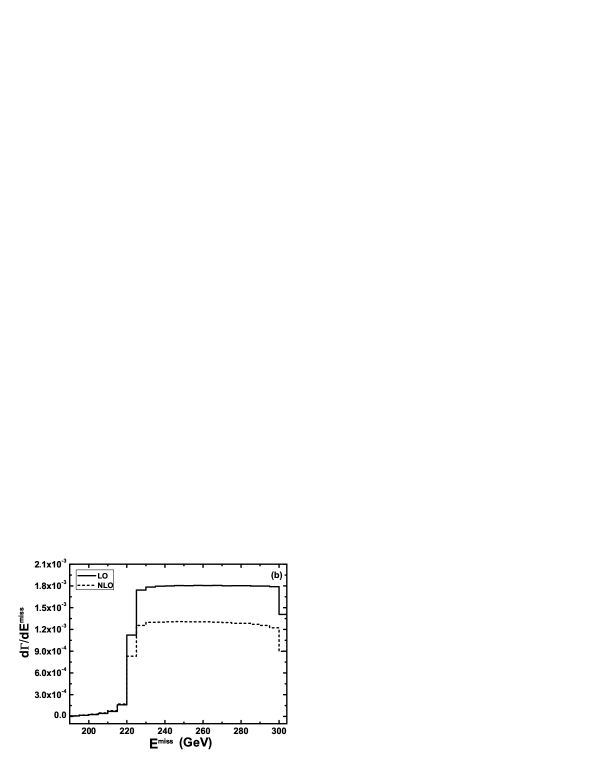
Figure 10: (a) The $t\bar{t}$ invariant mass distributions at the LO and the QCD NLO ($\frac{d\Gamma_{LO}}{dM_{t\bar{t}}}$, $\frac{d\Gamma_{NLO}}{dM_{t\bar{t}}}$) for the ${\rm SPS6}$ parameter set in Table 1. (b) The missing energy distributions at the LO and the QCD NLO ($\frac{d\Gamma_{LO}}{dE^{miss}}$, $\frac{d\Gamma_{NLO}}{dE^{miss}}$) with the ${\rm SPS6}$ parameter set listed in Table 1.

V Summary

In this paper we calculate the NLO QCD corrections to the decay process $\tilde{g}\to t\bar{t}\tilde{\chi}^{0}_{1}~{}$in the MSSM. As a numerical demonstration we present and discuss the NLO QCD corrections around the ${\rm SPS6}$ benchmark point. We find that the NLO QCD corrections significantly suppress the corresponding LO decay width, and at the scenario ${\rm SPS6}$ point the LO and the NLO QCD corrected decay widths have the values of $0.1490~{}GeV$ and $0.1069~{}GeV$ respectively, and the corresponding relative correction is $-28.2\%$. We analyze the dependence of the NLO QCD corrected decay width and the corresponding relative correction on the ratio of the vacuum expectation values, gluino mass, scalar top-quark masses and the lightest neutralino mass, respectively, around the scenario point ${\rm SPS6}$. Our numerical results show that the absolute NLO QCD relative correction can exceed $30\%$ in our chosen parameter space. Therefore, it is necessary to take the NLO QCD corrections into account for the precise experimental measurement at future colliders. We compare the distributions of the $t\bar{t}$ invariant mass and the missing energy at the LO and the QCD NLO and find that the line shapes of the differential decay widths at the LO, $\frac{d\Gamma_{LO}}{dM_{t\bar{t}}}$ and $\frac{d\Gamma_{LO}}{dE^{miss}}$, are not obviously changed by the NLO QCD corrections.

Acknowledgments: This work was supported in part by the National Natural Science Foundation of China (Contract No.11075150, No.11005101), and the Specialized Research Fund for the Doctoral Program of Higher Education (Contract No.20093402110030).

References

• [1] H. P. Nilles, Phys. Rept. 110 (1984) 1; H. E. Haber and G. Kane, Phys. Rept. 117 (1985) 75; R. Arnowitt and P. Nath, CTP-TAMU-52/93; M. Drees and S. Martin, MAD-PH-879, UM-TH-95-02, arXiv:hep-ph/9504324; J. Bagger, JHU-TIPAC-96008, arXiv:hep-ph/9604232; P.M. Zerwas et al., KA-TP-16-96, arXiv:hep-ph/9605437.
• [2] R. M. Barnett, J. F. Gunion and H. E. Haber, Phys. Rev. D37 (1988) 1892.
• [3] J. Hisano, K. Kawagoe and M. M. Nojiri, Phys. Rev. D68 (2003) 035007.
• [4] M. Toharia and J. D. Wells, J. High Energy Phys. 0602 (2006) 015.
• [5] A. Bartl, W. Majerotto, B. MΓΆsslacher, N. Oshimo and S. Stippel, Phys. Rev. D43 (1991) 2214.
• [6] S. Heinemeyer and C. Schappacher, KA-TP-40-2011, arXiv:1112.2830[hep-ph].
• [7] J. Fan, D. Krohn, P. Mosteiro, A. M. Thalapillil and L. T. Wang, J. High Energy Phys. 1103 (2011) 077.
• [8] ATLAS collaboration, ATLAS-CONF-2012-033
• [9] CMS Collaboration, Report No.CMS-PAS-SUS-11-016.
• [10] J. Berger, M. Perelstein, M. Saelim, and A. Spray, arXiv:1111.6594[hep-ph].
• [11] J. A. Aguilar-Saavedra, et al., Eur. Phys. J. C 46, 43 (2006), arXiv:hep-ph/0511344.
• [12] B. C. Allanach et al., Eur. Phys. J. C 25, 113 (2002), arXiv:hep-ph/0202233.
• [13] A. Denner, S. Dittmaier, M. Roth and D. Wackeroth, Nucl. Phys. B560 (1999) 33; A. Denner, S. Dittmaier, M. Roth and L.H. Wieders, Nucl. Phys. B724 (2005) 247.
• [14] T. Hahn, Comput. Phys. Commun. 140 (2001) 418.
• [15] T. Hahn and M. Perez-Victoria, Comput. Phys. Commun. 118 (1999) 153.
• [16] D. Choudhury, S. Majhi and V. Ravindran, Nucl. Phys. B660 (2003) 343.
• [17] R.K. Ellis and G. Zanderighi, JHEP 0802 (2008) 002.
• [18] G. ’t Hooft and M. Veltman, Nucl. Phys. B153 (1979) 365; A. Denner, U. Nierste and R. Scharf, Nucl. Phys. B367 (1991) 637; A. Denner and S. Dittmaier, Nucl. Phys. B658 (2003) 175.
• [19] G. J. van Oldenborgh, Comput. Phys. Commun. 66 (1991) 1.
• [20] A. Denner and S. Dittmaier, Nucl. Phys B844 (2011)199, arXiv:1005.2076.
• [21] A. Denner, Fortschr. Phys. 41 (1993) 307.
• [22] K. I. Aoki et al., Prog. Theor. Phys. 65 (1981) 1001; Prog. Theor. Phys. Suppl. 73 (1982) 1.
• [23] M. BΓΆhm, H. Spiesberger and W. Hollik, Fortschr. Phys. 34 (1986) 687; W. Hollik, Fortschr. Phys. 38 (1990) 165.
• [24] J. Collins, F. Wilczek and A. Zee, Phys. Rev. D18 (1978) 242; W. J. Marciano, Phys. Rev. D29 (1984) 580; P. Nason, S. Dawson and R.K. Ellis, Nucl. Phys. B327 (1989) 49; Nucl. Phys. B335 (1990) 260(E).
• [25] W. Beenakker, R. HΓΆpker and P. M. Zerwas, Phys. Lett. B378 (1996) 159; W. Beenakker, R. HΓΆpker, T. Plehn and P.M. Zerwas, Z. Phys. C75 (1997) 349.
• [26] S. Berge, W. Hollik, W.M. Mosle and D. Wackeroth, Phys. Rev. D76 (2007) 034016.
• [27] W. T. Giele and E. W. N. Glover, Phys. Rev. D46 (1992) 1980; W. T. Giele, E. W. Glover and D. A. Kosower, Nucl. Phys. B403 (1993) 633; S. Keller and E. Laenen, Phys. Rev. D59 (1999) 114004.
• [28] G. P. Lepage, J. Comput. Phys. 27 (1978) 192.
• [29] W. Beenakker, S. Dittmaier, M. Kramer, B. Plumper, M. Spira and P. M. Zerwas, Phys. Rev. Lett. 87 (2001) 201805; Nucl. Phys. B653 (2003) 151.
• [30] S. Catani and M. H. Seymour, Phys. Lett. B378 (1996) 287; Nucl. Phys. B485 (1997) 291.
• [31] S. Catani, S. Dittmaier, M. H. Seymour and Z. TrΓ³csΓ‘nyi, Nucl. Phys. B627 (2002) 189.
• [32] L. Reina, S. Dawson and D. Wackeroth, Phys. Rev. D65 (2002) 053017.
• [33] K. Nakamura, et al., J. Phys. G37 (2010) 075021.
• [34] G. Aad, et al. [ATLAS Collaboration], arXiv:hep-ex/1109.6572.
• [35] ATLAS report, ATLAS-CONF-2011-163; CMS report, CMS-PAS-HIG-11-032.
• [36] Nabil Ghodbane, Hans-Ulrich Martyn, ’Compilation of SUSY particle spectra from Snowmass 2001 benchmark models’, arXiv:hep-ph/0201233.
• [37] http://www.nhn.ou.edu/$\sim$isajet/