Distance Distributions in Regular Polygons

Abstract

This paper derives the exact cumulative density function of the distance between a randomly located node and any arbitrary reference point inside a regular $L$-sided polygon. Using this result, we obtain the closed-form probability density function (PDF) of the Euclidean distance between any arbitrary reference point and its $n$-th neighbour node, when $N$ nodes are uniformly and independently distributed inside a regular $L$-sided polygon. First, we exploit the rotational symmetry of the regular polygons and quantify the effect of polygon sides and vertices on the distance distributions. Then we propose an algorithm to determine the distance distributions given any arbitrary location of the reference point inside the polygon. For the special case when the arbitrary reference point is located at the center of the polygon, our framework reproduces the existing result in the literature.

I Introduction

Recently, the distance distributions in wireless networks have received a lot of attention in the literature [1, 2, 3]. The distance distributions can be applied to study important wireless network characteristics such as interference, outage probability, connectivity, routing and energy consumption [1, 4, 5, 6]. The distance distributions in wireless networks are dependent on the location of the nodes, which are seen as realizations of some spatial point process. When the node locations follows an infinite homogeneous Poisson point process, the probability density function (PDF) of the Euclidean distance between a point and its $n$-th neighbour node follows a generalised Gamma distribution [7]. However, as recently identified in [1, 2, 8, 9], this model does not accurately reflect the distance distributions in many practical wireless networks where a fixed and finite number of nodes are uniformly and independently distributed over a finite area such as square or hexagon or disk region. Note that these finite regions of interest can be conveniently modeled as special cases of a regular $L$-sided polygon (referred to as $L$-gon for brevity), e.g., $L=3,4,6,\infty$ correspond to equilateral triangle, square, hexagon and disk respectively. In this context, the two important distance distributions are: (i) the PDF of the Euclidean distance between two nodes uniformly and independently distributed inside a $L$-gon and (ii) the PDF of the Euclidean distance between any arbitrary reference point and its $n$-th neighbour node, when $N$ nodes are uniformly and independently distributed inside a $L$-gon. For the first case, the PDF of the distance between two nodes uniformly and independently distributed inside an equilateral triangle [10], square [11, 12], hexagon [13, 3] and disk [11] are well known in the literature. These results are special cases of the general result obtained recently in [14]. For the second case, the PDF of the Euclidean distance to the $n$-th neighbour node is obtained in [1] for the special case when the reference point is located at the center of the $L$-gon.

In this correspondence, we present a general framework for analytically obtaining the exact cumulative density function of the distance between a randomly located node and any arbitrary reference point inside a regular $L$-sided polygon. Using this result, we obtain the closed-form PDF of the Euclidean distance between any arbitrary reference point and its $n$-th neighbour node, when $N$ nodes are uniformly and independently distributed inside a regular $L$-sided polygon. The proposed framework is based on characterising the overlap area between the $L$-gon and a disk centered at the arbitrary reference point located inside the $L$-gon. There are two key insights which lead to our results: the use of the rotation operator that simplifies the characterisation of distances and overlap areas, and the systematic analysis of the effect of $L$-gon sides and vertices on the overlap area. Based on our proposed framework, we formulate an algorithm to determine the distance distributions given any location of the reference point inside the polygon. We provide examples to demonstrate the generality of our proposed framework. We also show that the result in [1] can be obtained as a special case in our framework.

II System Model

Consider $N$ nodes which are uniformly and independently distributed inside a regular $L$-sided polygon $\mathcal{A}\in\mathbb{R}^{2}$, where $\mathbb{R}^{2}$ denotes the two dimensional Euclidean domain. Let $\boldsymbol{u}=[x,\,y]^{T}\in\mathcal{A}$ denote an arbitrary reference point located inside the $L$-gon, where $[\cdot]^{T}$ denotes transpose of a vector.

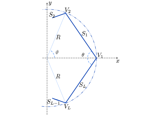
Figure 1: Illustration of sides, vertices and angles for the $L$-sided polygon inscribed in a circle of radius $R$. $\theta$ denoting the interior angle of the polygon and $\vartheta$ denoting the central angle between two adjacent vertices are defined in (2).

II-A Polygon geometry

Without loss of generality, we assume that the $L$-gon is inscribed in a circle of radius $R$ and is centered at the origin $[0,\,0]^{T}$. Then, its inradius is $R_{\textrm{i}}=R\cos(\pi/\ell)$ and its area $A$ is given by

$$A=|\mathcal{A}|=\frac{1}{2}LR^{2}\sin\left(\frac{2\pi}{L}\right).$$ (1)

Let $S_{\ell}$ and $V_{\ell}$ denotes the sides and vertices of the polygon, for $\ell=1,2,\ldots,L$, which are numbered in anti-clockwise direction, as shown in Fig. 1. We assume that the first vertex $V_{1}$ of the polygon is at $[R,\,0]^{T}$, i.e., at the intersection of the circle inscribing the polygon and the $x$-axis. The interior angle of the polygon $\theta$ and the central angle between two adjacent vertices $\vartheta$ are given by

$$\theta =\frac{\pi(L-2)}{L}\qquad\textrm{and}\qquad\vartheta=\frac{2\pi}{L}.$$ (2)

II-B Rotation operator

For compact representation, we define the rotation operator $\mathfrak{R}^{\ell}$ which rotates an arbitrary point $\boldsymbol{u}=[x,\,y]^{T}$ anti-clockwise around the origin by an angle $\ell\vartheta$. The rotated point $\mathfrak{R}^{\ell}\boldsymbol{u}$ can thus be expressed as

$$(\mathfrak{R}^{\ell}\boldsymbol{u})=\mathbf{T}\,\boldsymbol{u},$$ (3)

where $\mathbf{T}$ is the corresponding rotation matrix of $\mathfrak{R}^{\ell}$ and is given by

$$\mathbf{T}\,=\,\left(\begin{array}[]{cc}\cos(\ell\vartheta)&-\sin(\ell\vartheta)\\ \sin(\ell\vartheta)&\cos(\ell\vartheta)\end{array}\right).$$ (6)

Also define $\mathfrak{R}^{-\ell}$ as the inverse rotation operator with rotation matrix $\mathbf{T}^{-1}$, which rotates an arbitrary point $\boldsymbol{u}=[x,\,y]^{T}$ clockwise around the origin by an angle $\ell\vartheta$. We note that the rotation under the operator $\mathfrak{R}$ is an isometric operation which preserves the distances between any two points in the two dimensional plane, i.e., $\det(\mathbf{T})=1$ and $\mathbf{T}\mathbf{T}^{-1}=\mathbf{I}$, where $\mathbf{I}$ denotes the identity matrix.

II-C Distances from the polygon sides and vertices

In this subsection, we find the distances from an arbitrary reference point $\boldsymbol{u}$ located inside the polygon to all its sides and vertices. First, we examine the distance to any vertex. Using the geometry, the distance $d(\boldsymbol{u};\,V_{1})$ between the point $\boldsymbol{u}$ and the vertex $V_{1}$ is given by

$$d(\boldsymbol{u};\,V_{1})\, =\,\sqrt{(x-R)^{2}+y^{2}}.$$ (7)

In order to find the distances to the remaining vertices, we use $d(\boldsymbol{u};\,V_{1})$ and exploit the rotational symmetry of the $L$-gon. By appropriately rotating the point $\boldsymbol{u}$ and then finding its distance from vertex $V_{1}$, we can in fact, find the distance to other vertices. Thus, using (7) and the rotation operator defined in (3), we can express $d(\boldsymbol{u};\,V_{\ell})$ as

$$d(\boldsymbol{u};\,V_{\ell})\, =\,d(\mathfrak{R}^{-(\ell-1)}\boldsymbol{u};\,V_{1}).$$ (8)

Next, we examine the distance to any side. We define this distance to any side as the shortest distance between the point $\boldsymbol{u}$ and the line segment formed by the side of the polygon. If the projection of the point $\boldsymbol{u}$ onto a side lies inside the side, then the shortest distance is given by the perpendicular distance between the point and the side. If the projection of the point $\boldsymbol{u}$ onto a side does not lie on the side, then the shortest distance is the minimum of the distance to the side endpoints. Using the geometry, the perpendicular distance from an arbitrary point $\boldsymbol{u}$ to the line segment formed by side $S_{1}$ is given by

$$p(\boldsymbol{u};\,S_{1})\, =\,\frac{\textrm{abs}\left(y+\tan\left(\frac{\theta}{2}\right)\,x-R\tan\left(\frac{\theta}{2}\right)\right)}{\sqrt{1+\tan^{2}\left(\frac{\theta}{2}\right)}},$$ (9)

where $\mathrm{abs}(\cdot)$ denotes the absolute value. The distance to the side $S_{1}$ endpoints is simply given by $d(\boldsymbol{u};\,V_{1})$ and $d(\boldsymbol{u};\,V_{2})$. Thus, the shortest distance $d(\boldsymbol{u};\,S_{1})$ to the side $S_{1}$ can be expressed as

$$d(\boldsymbol{u};\,S_{1})\, =\,\begin{cases}\min(d(\boldsymbol{u};\,V_{1}),\,d(\boldsymbol{u};\,V_{2})),&\max(d(\boldsymbol{w};V_{1}),\,d(\boldsymbol{w};V_{2}))>t;\\ p(\boldsymbol{u};\,S_{1}),&\textrm{otherwise};\end{cases}$$ (10)

where $\boldsymbol{w}=\big{[}R-\frac{(x-R)(\cos\vartheta-1)+y\sin\vartheta}{2},\,\frac{\sin\vartheta\big{(}(x-R)(\cos\vartheta-1)+y\sin\vartheta\big{)}}{2(1-\cos\vartheta)}\big{]}^{T}$ denotes the perpendicular projection of $\boldsymbol{u}$ onto the line segment formed by side $S_{1}$, $t=2R\sin\left(\frac{\pi}{L}\right)$ is the side length of the $L$-gon and $\min(\cdot)$ and $\max(\cdot)$ denote the minimum and maximum values respectively. Then, using (3), we can express $p(\boldsymbol{u};\,S_{\ell})$ and $d(\boldsymbol{u};\,S_{\ell})$ as

$$p(\boldsymbol{u};\,S_{\ell})\,=\,p(\mathfrak{R}^{-(\ell-1)}\boldsymbol{u};\,S_{1}),\quad d(\boldsymbol{u};\,S_{\ell})\,=\,d(\mathfrak{R}^{-(\ell-1)}\boldsymbol{u};\,S_{1}),$$ (11)

Definition 1

Define the distance vector $\mathbf{d}$ as an indexed vector of the distances from the arbitrary point $\boldsymbol{u}\in\mathcal{A}$ to all the sides and vertices of the $L$-gon, defined in (7), (8), (10), and (11) as

$$\mathbf{d}\,=\,[d(\boldsymbol{u};S_{1}),\,\ldots,\,d(\boldsymbol{u};S_{L}),\,d(\boldsymbol{u};V_{1}),\,\ldots,\,d(\boldsymbol{u};V_{L})].$$ (12)

III Problem Formulation

Consider a disk $\mathcal{D}(\boldsymbol{u};r)$ of radius $r$ centered at the arbitrary reference point $\boldsymbol{u}$. First, we define the probability that a random node, which is uniformly distributed inside the $L$-gon $\mathcal{A}$, lies at a distance of less than or equal to $r$ from the point $\boldsymbol{u}$.

Definition 2

Define the cumulative density function (CDF) $F(\boldsymbol{u};r)$, which is the probability that a random node falls inside a disk $\mathcal{D}(\boldsymbol{u};r)$ of radius $r$ centered at the arbitrary reference point $\boldsymbol{u}$, as

$$F(\boldsymbol{u};r)\, =\,\frac{|\mathcal{D}(\boldsymbol{u};r)\cap\mathcal{A}|}{|\mathcal{A}|}=\frac{O(\boldsymbol{u};r)}{A}$$ (13)

where $O(\boldsymbol{u};r)=|\mathcal{D}(\boldsymbol{u};r)\cap\mathcal{A}|$ is the overlap area between the disk $\mathcal{D}(\boldsymbol{u};r)$ and $L$-gon $\mathcal{A}$.

Then the PDF $f_{n}(\boldsymbol{u};r)$ of the distance from an arbitrary point $\boldsymbol{u}$ to the $n$-th neighbour node is [1]

$$f_{n}(\boldsymbol{u};r)\,=\,\frac{\big{(}1-F(\boldsymbol{u};r)\big{)}^{N-n}\big{(}F(\boldsymbol{u};r)\big{)}^{n-1}}{B(N-n+1,k)}\,\frac{\partial\,F(\boldsymbol{u};r)}{\partial r}$$ (14)

where $N$ is the number nodes are which are uniformly and independently distributed inside the $L$-gon, $B(a,b)=\Gamma(a)\Gamma(b)/\Gamma(a+b)$ is the beta function, $\Gamma(\cdot)$ denotes the gamma function, $\frac{\partial}{\partial r}(\cdot)$ denotes the partial derivative respect to the variable $r$ and $F(\boldsymbol{u};r)$ is given in (13).

The challenge in evaluating (13) and (14) is finding the overlap area $O(\boldsymbol{u};r)$. When the reference point is located at the center of the $L$-gon, the overlap area $O(\boldsymbol{u};r)$ can be easily evaluated as shown in [1]. For $0\leq r\leq R_{\textrm{i}}$ (where $R_{\textrm{i}}$ is the $L$-gon inradius defined above (1)), the disk $\mathcal{D}(\boldsymbol{u};r)$ is entirely inside the $L$-gon $\mathcal{A}$. Thus the overlap area is the same as the area of the disk, i.e, $O(\boldsymbol{u};r)=\pi r^{2}$. For $R_{\textrm{i}}\leq r\leq R$, (where $R$ is the $L$-gon circumradius) there are $L$ circular segment shaped portions of the disk $\mathcal{D}(\boldsymbol{u};r)$ which are outside the $L$-gon. Since these circular segments are symmetric and there is no overlap between them, the overlap area is given by $O(\boldsymbol{u};r)=\pi r^{2}-L(\textrm{area of one circular segment})$. Note that in this case it is simple to find the area of one circular segment using geometry.

When the reference point is not located at the center, then the circular segments are no longer symmetric. This is illustrated in Fig. 2 for the case of a square ($L=4$) for simplicity. We can see that for the given radius of the disk $\mathcal{D}(\boldsymbol{u};r)$ centered at the reference point, non-symmetric circular segment areas are formed outside the sides $S_{1}$, $S_{2}$ and $S_{4}$. In addition, there is overlap between the circular segment areas formed outside the sides $S_{1}$ and $S_{2}$. This complicates the task of finding the overlap area $O(\boldsymbol{u};r)$. Also, for any arbitrary location of the reference point, the different ranges for $r$ are no longer exclusively determined by the inradius $R_{\textrm{i}}$ and circumradius $R$, but by the number of unique distances from the reference point to the vertices and the sides. This adds further complexity to the task of finding the overlap area $O(\boldsymbol{u};r)$.

In the next section, we propose our method to systematically account for the effect of sides and vertices on the overlap area $O(\boldsymbol{u};r)$. Then in Section V, we propose an algorithm to automatically formulate the different ranges for $r$ and find the overlap area $O(\boldsymbol{u};r)$ in order to evaluate (13) and (14).

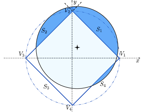
Figure 2: Illustration of the non-symmetric circular segment areas formed outside the sides $S_{1}$, $S_{2}$ and $S_{4}$ for a square ($L=4$-gon). There is also an overlap between the circular segment areas formed outside the sides $S_{1}$ and $S_{2}$.

IV Characterization of the Effect of Sides and Vertices

In this section, we characterize the effect of polygon sides and vertices on the overlap area $O(\boldsymbol{u};r)$. Because of the symmetry of the polygon, we only need to consider the following three cases which are illustrated in Fig. 3. Other cases can be handled as an appropriate combination of these cases:

1. The overlap area is limited by one side of the polygon only. This is illustrated in Fig. 3(a) for side $S_{1}$.

2. The overlap area is limited by two sides of the polygon and there is no overlap between them. This is illustrated in Fig. 3(b) for sides $S_{1}$ and $S_{L}$.

3. The overlap area is limited by two sides of the polygon and there is overlap between them. This is illustrated in Fig. 3(c) for side $S_{1}$ and $S_{L}$ and vertex $V_{1}$.

These cases are discussed in detail in the following subsections.

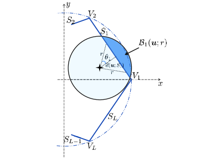
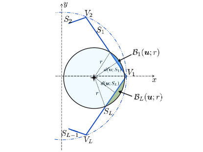
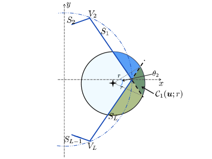
Figure 3: Illustration of the effect of sides and vertices of the polygon on the overlap are: (a) overlap area is limited by side $S_{1}$, (b) overlap area is limited by sides $S_{1}$ and $S_{L}$ only and (c) overlap area is limited by sides $S_{1}$ and $S_{L}$ with inclusion of the vertex $V_{1}$.

IV-A Case 1: Overlap area limited by one side only

Let $\mathcal{B}_{1}(\boldsymbol{u};r)$ denote the circular segment formed outside the side $S_{1}$, as shown in Fig. 3(a). It is obvious that the overlap area in this case is given by $O(\boldsymbol{u};r)=\pi r^{2}-B_{1}(\boldsymbol{u};r)$, where $B_{1}(\boldsymbol{u};r)=|\mathcal{B}_{1}(\boldsymbol{u};r)|$. Using polar coordinates, we can find the area $B_{1}(\boldsymbol{u};r)$ by integrating the angle $\theta_{1}$ (shown in Fig. 3(a)) over $\mathcal{B}_{1}(\boldsymbol{u};r)$ as

$$B_{1}(\boldsymbol{u};r)\, =\,\|\mathcal{B}_{1}(\boldsymbol{u};r)\|$$

$$=\,2\int_{d(\boldsymbol{u};S_{1})}^{r}\,r^{\prime}\arccos\left(\frac{p(\boldsymbol{u};S_{1})}{r^{\prime}}\right)dr^{\prime}$$

$$=\,\begin{cases}r^{2}\arccos\left(\frac{p(\boldsymbol{u};S_{1})}{r}\right)-(d(\boldsymbol{u};S_{1}))^{2}\arccos\left(\frac{p(\boldsymbol{u};S_{1})}{d(\boldsymbol{u};S_{1})}\right)-\\ \quad p(\boldsymbol{u};S_{1})\bigg{(}\sqrt{r^{2}-\big{(}p(\boldsymbol{u};S_{1})\big{)}^{2}}-\sqrt{(d(\boldsymbol{u};S_{1}))^{2}-\big{(}p(\boldsymbol{u};S_{1})\big{)}^{2}}\bigg{)},\,\,&r\geq d(\boldsymbol{u};S_{1});\\ 0,\,\,&\textrm{otherwise};\\ \end{cases}$$ (15)

where $p(\boldsymbol{u};S_{1})$ and $d(\boldsymbol{u};S_{1})$ are given in (9) and (10) respectively.

Generalizing, let $\mathcal{B}_{\ell}(\boldsymbol{u};r)$ denote the circular segment which is formed outside the side $S_{\ell}$. Using (IV-A) and the rotation operator in (3), we can express $B_{\ell}(\boldsymbol{u};r)$ as

$$B_{\ell}(\boldsymbol{u};r)\, =\,\begin{cases}B_{1}(\mathfrak{R}^{-(\ell-1)}\boldsymbol{u};r),\,\,&r\geq d(\boldsymbol{u};S_{\ell});\\ 0,\,\,&\textrm{otherwise}.\\ \end{cases}$$ (16)

IV-B Case 2: Overlap area limited by two sides with no overlap

This case is illustrated in Fig. 3(b), where two circular segments, $\mathcal{B}_{1}(\boldsymbol{u};r)$ and $\mathcal{B}_{L}(\boldsymbol{u};r)$, are formed outside the sides $S_{1}$ and $S_{L}$, respectively. Since there is no overlap between the circular segments, the overlap area is given by $O(\boldsymbol{u};r)=\pi r^{2}-(B_{1}(\boldsymbol{u};r)+B_{L}(\boldsymbol{u};r))$, where $B_{1}(\boldsymbol{u};r)$ is given by (IV-A) and $B_{L}(\boldsymbol{u};r)$ can be found using (16).

IV-C Case 3: Overlap area limited by two sides with overlap

This case is illustrated in Fig. 3(c), where there is overlap between the two circular segments, $\mathcal{B}_{1}(\boldsymbol{u};r)$ and $\mathcal{B}_{L}(\boldsymbol{u};r)$, formed outside sides $S_{1}$ and $S_{L}$ due to the inclusion of the vertex $V_{1}$. Let $\mathcal{C}_{1}(\boldsymbol{u};r)=\mathcal{B}_{1}(\boldsymbol{u};r)\cap\mathcal{B}_{L}(\boldsymbol{u};r)$ denote this overlap region between the two circular segments. Thus, in this case, the overlap area is given by $O(\boldsymbol{u};r)=\pi r^{2}-(B_{1}(\boldsymbol{u};r)+B_{L}(\boldsymbol{u};r)-C_{1}(\boldsymbol{u};r))$.

Using polar coordinates, we can find the area $C_{1}(\boldsymbol{u};r)$ by integrating the angle $\theta_{2}$ (shown in Fig. 3(c)) over $\mathcal{C}_{1}(\boldsymbol{u};r)$ as

$$C_{1}(\boldsymbol{u};r) =\|\mathcal{C}_{1}(\boldsymbol{u};r)\|$$

$$=\int_{d(\boldsymbol{u};V_{1})}^{r}\,r^{\prime}\bigg{(}\frac{\pi(L-2)}{L}+\arccos\left(\frac{p(\boldsymbol{u};S_{1})}{r^{\prime}}\right)+\arccos\left(\frac{p(\boldsymbol{u};S_{L})}{r^{\prime}}\right)-\pi\bigg{)}dr^{\prime}$$

$$=\begin{cases}\frac{r^{2}}{2}\left(\arccos\left(\frac{p(\boldsymbol{u};S_{1})}{r}\right)\,+\,\arccos\left(\frac{p(\boldsymbol{u};S_{L})}{r}\right)\right)\,-\,\\ \frac{{(d(\boldsymbol{u};V_{1}))}^{2}}{2}\left(\arccos\left(\frac{p(\boldsymbol{u};S_{1})}{d(\boldsymbol{u};V_{1})}\right)+\arccos\left(\frac{p(\boldsymbol{u};S_{L})}{d(\boldsymbol{u};V_{1})}\right)\right)\,+\,\\ \frac{p(\boldsymbol{u};S_{1})}{2}\left(\sqrt{\big{(}d(\boldsymbol{u};V_{1})\big{)}^{2}-\big{(}p(\boldsymbol{u};S_{1})\big{)}^{2}}-\sqrt{r^{2}-\big{(}p(\boldsymbol{u};S_{1})\big{)}^{2}}\right)\,+\,\\ \frac{p(\boldsymbol{u};S_{L})}{2}\left(\sqrt{\big{(}d(\boldsymbol{u};V_{1})\big{)}^{2}-\big{(}p(\boldsymbol{u};S_{L})\big{)}^{2}}-\sqrt{r^{2}-\big{(}p(\boldsymbol{u};S_{L})\big{)}^{2}}\right)\,-\\ \frac{\pi}{L}\left(r^{2}-\big{(}d(\boldsymbol{u};V_{1})\big{)}^{2}\right),\,\,&r\geq d(\boldsymbol{u};V_{1});\\ 0,\,\,&\textrm{otherwise};\end{cases}$$ (17)

where $d(\boldsymbol{u};V_{1})$, $p(\boldsymbol{u};S_{1})$ and $p(\boldsymbol{u};S_{L})$ are given in (7), (9) and (11) respectively.

Generalizing, let $\mathcal{C}_{\ell}(\boldsymbol{u};r)$ denote the overlap region between two circular segments adjoining the vertex $V_{\ell}$ of the polygon. Using (IV-C) and the rotation operator in (3), we can express $C_{\ell}(\boldsymbol{u};r)$ as

$$C_{\ell}(\boldsymbol{u};r)\, =\,\begin{cases}C_{1}(\mathfrak{R}^{-(\ell-1)}\boldsymbol{u};r),\,\,&r\geq d(\boldsymbol{u};V_{\ell});\\ 0,\,\,&\textrm{otherwise}.\\ \end{cases}$$ (18)

The expressions for the derivatives of $B_{\ell}(\boldsymbol{u};r)$ and $C_{\ell}(\boldsymbol{u};r)$, which are needed in the evaluation of $\frac{\partial F(\boldsymbol{u};r)}{\partial r}$ in (14), are provided in Appendix A.

V Distance Distributions in Polygons

In this section, we present our algorithm to use the distance vector in (12) and the effect of different sides and vertices ((IV-A)$-$(18)) in order to find the overlap area $O(\boldsymbol{u};r)$ given any arbitrary reference point $\boldsymbol{u}=[x,\,y]^{T}$ located inside the $L$-gon $\mathcal{A}$.

The overall effect of the sides and vertices of the $L$-gon depends on the range of the distance $r$ and on the distance between the reference point and all the sides and vertices. Since an $L$-gon has $L$ sides and $L$ vertices, there can be $2L+1$ different ranges for the distance $r$. We sort the distance vector $\mathbf{d}$ in (12) in ascending order and define $\acute{\mathbf{d}}$ to be the sorted distance vector. Then, the first range of the distance is $0\leq r\leq\acute{d}_{1}$, where $\acute{d}_{1}$ denotes the first entry of the sorted distance vector $\acute{\mathbf{d}}$. The next $2L-1$ ranges are $\acute{d}_{j}\leq r\leq\acute{d}_{j+1},\,j=2,\,3,\ldots,\,2L$ and the last range is $\acute{d}_{2L}\leq r$. Thus, in general, we can write an expression for $O(\boldsymbol{u};r)$ as

$$O(\boldsymbol{u};r)=\begin{cases}O_{1}(\boldsymbol{u};r)=\pi r^{2},\,\,&0\leq r\leq\acute{d}_{1};\\ O_{2}(\boldsymbol{u};r),\,\,&\acute{d}_{1}\leq r\leq\acute{d}_{2};\\ \,\,\vdots&\,\,\vdots\\ O_{2L}(\boldsymbol{u};r),\,\,&\acute{d}_{2L-1}\leq r\leq\acute{d}_{2L};\\ O_{2L+1}(\boldsymbol{u};r)=A,\,\,&r\geq\acute{d}_{2L};\\ \end{cases}$$ (19)

where the subscript $j$ in $O_{j}(\boldsymbol{u};r)$ denotes the overlap area for the $j$-th range.

For the first range $0\leq r\leq\acute{d}_{1}$, $S_{1}(\boldsymbol{u};r)\,=\pi r^{2}$, since the disk $\mathcal{D}(\boldsymbol{u};r)$ will be completely inside the $L$-gon. For the last range $\acute{d}_{2L}\leq r$, $O_{2L+1}(\boldsymbol{u};r)=A$, since the disk $\mathcal{D}(\boldsymbol{u};r)$ will completely overlap with the $L$-gon $\mathcal{A}$. For the intermediate ranges, the overlap area may be limited by any number of sides, with or without overlap between any two adjacent sides. Also depending on the location of the arbitrary reference point, some of the distance to the sides and vertices may be the same. In order to automate the process of finding the unique set of ranges for the distance $r$ and to calculate the corresponding overlap area for each unique range, we propose the Algorithm 1.

Algorithm 1 Algorithm to find the overlap area

  Step 1: Sort ${\mathbf{d}}$ in (12) in ascending order to obtain $\acute{\mathbf{d}}$

  Step 2: Determine the index sorting that transforms ${\mathbf{d}}$ into $\acute{\mathbf{d}}$ and obtain the index vector $\mathbf{k}$

  Step 3: Find the appropriate circular segment areas and the overlap area

  for each $j$ in $j=1,2,3,\ldots,2L+1$ do

     if $\acute{d}_{j-1}-\acute{d}_{j}\neq 0$, ($\acute{d}_{0}=0)$ then

        $O_{j}(\boldsymbol{u};r)=\pi r^{2}$

        for each $i$ in $i=1,2,3,\ldots,j-1$ do

           if ${k}_{i}\leq L$ then

              $O_{j}(\boldsymbol{u};r)=O_{j}(\boldsymbol{u};r)-B_{k_{i}}(\boldsymbol{u};r)$

           else

              $O_{j}(\boldsymbol{u};r)=O_{j}(\boldsymbol{u};r)+C_{k_{i}-L}(\boldsymbol{u};r)$

           end if

        end for

     end if

  end for

  

In the proposed algorithm, we sort the distance vector $\mathbf{d}$ in (12) in ascending order to obtain the sorted distance vector $\acute{\mathbf{d}}$ and the index vector $\mathbf{k}=[k_{1},\,k_{2},\,\ldots,\,k_{2L}]$. The index vector $\mathbf{k}$ is then used to find the effect of sides and vertices on the overlap area for each value of range. For each unique range $\acute{d}_{j-1}-\acute{d}_{j}$ which is determined in the outer for loop, we evaluate the overlap area $O_{j}(\boldsymbol{u};r)$ in (19) in the inner for loop by taking into account the cumulative effect of all of the sides and vertices. The terms $B_{L}(\boldsymbol{u};r)$ and $C_{L}(\boldsymbol{u};r)$ are appropriately selected using the index vector $\mathbf{k}$. Once $O(\boldsymbol{u};r)$ in (19) is computed for each unique range, it can then used to evaluate (13) and (14). We have implemented the proposed algorithm in MATLAB.

V-A Algorithm illustration - arbitrary reference point in a square

In order to illustrate the proposed framework and algorithm, we consider the problem to find CDF in (13) and the PDF in (14) for a point $\boldsymbol{u}_{1}=[R/2,\,-R/2]^{T}$ located in the middle of the side $S_{4}$ of the square ($L=4$). The distance vector $\mathbf{d}$ in (12) and the sorted distance vector $\acute{\mathbf{d}}$ are given by

$$\mathbf{d}\, =\,\left[\frac{R}{\sqrt{2}},\,\sqrt{2}R,\,\frac{R}{\sqrt{2}},\,0,\,\frac{R}{\sqrt{2}},\,\frac{\sqrt{10}R}{2},\,\frac{\sqrt{10}R}{2},\,\frac{R}{\sqrt{2}}\right],$$

$$\acute{\mathbf{d}}\, =\,\left[0,\,\frac{R}{\sqrt{2}},\,\frac{R}{\sqrt{2}},\,\frac{R}{\sqrt{2}},\,\frac{R}{\sqrt{2}},\,\sqrt{2}R,\,\frac{\sqrt{10}R}{2},\,\frac{\sqrt{10}R}{2}\right].$$

Thus the index vector ${\mathbf{k}}$ for this case is given by $\mathbf{k}\,=\,[4,\,1,\,2,\,5,\,8,\,3,\,6,\,7]$, which is employed to determine $O(\boldsymbol{u};r)$ in (19) using the proposed algorithm. Thus the CDF is

$$F(\boldsymbol{u}_{1};r)=\frac{1}{A}\begin{cases}\pi r^{2}-B_{4},\,\,&0\leq r\leq R/\sqrt{2};\\ \pi r^{2}-(B_{1}+B_{2}+B_{4}-C_{1}-C_{4}),\,\,&R/\sqrt{2}\leq r\leq\sqrt{2}R;\\ \pi r^{2}-(B_{1}+B_{2}+B_{3}+B_{4}-C_{1}-C_{4}),\,\,&\sqrt{2}R\leq r\leq\sqrt{10}R/2;\\ A,\,\,&r\geq\sqrt{10}R/2.\\ \end{cases}$$ (20)

Substituting (20), and its derivative which is obtained using the expressions in Appendix A, in (14), we obtain the PDF of the distance to the $n$-th neighbour, which is shown in Fig. 4 for $R=1$, $N=5$ and $n=1,\,2,\ldots,\,5$. We can see that the simulation results, which are averaged over 10,000 simulation runs, match perfectly with the analytical results, verifying the proposed framework and algorithm.

Figure 4: The PDF $f_{n}(\boldsymbol{u};r)$ of the distance to $n$-th nearest neighbour for a point located midway between the $V_{1}$ and $V_{4}$ on the side $S_{4}$ of the square ($L=4$). The circumradius $R=1$ and the number of nodes is $N=5$.

V-B Special case - reference point at the center of the polygon

Consider the special case that the reference point is located at the center $O$ of the polygon, i.e., at the origin $\boldsymbol{u}_{2}=[0\;0]^{T}$. All of the sides and also all of the vertices are equidistant from the center of the polygon and the rotation operator does not affect the point located at the origin. This implies that $d(\boldsymbol{u}_{2};S_{\ell})=d(\boldsymbol{u}_{2};S_{1})=R\tan(\theta/2)$, $d(\boldsymbol{u}_{2};V_{\ell})=d(\boldsymbol{u}_{2};V_{1})=R$, $B_{\ell}=B_{1}$ and $C_{\ell}=C_{1}$ for $\ell=2,3,\ldots,L$. By employing these relations and the proposed algorithm, we obtain the CDF expression for the following three possible ranges

$$F(\boldsymbol{u}_{2};r)\,=\,\frac{1}{A}\begin{cases}{\pi r^{2}},\,\,&0\leq r\leq R\tan\left(\frac{\theta}{2}\right);\\ {\pi r^{2}}-\,LB_{1},\,\,&R\tan\left(\frac{\theta}{2}\right)\leq r\leq R;\\ A,\,\,&r\geq R;\\ \end{cases}$$ (21)

where $B_{1}=r^{2}\arccos\big{(}\frac{R}{r}\tan\left(\frac{\theta}{2}\right)\big{)}-R\tan\frac{\theta}{2}\sqrt{r^{2}-R^{2}\tan^{2}\left(\frac{\theta}{2}\right)}$ and $\theta$ is defined in (2). Substituting (21) in (14) reproduces the result in [1].

V-C Special case - reference point at the vertex of the polygon

Consider the special case when the arbitrary point is located at one of the vertex of the polygon. Let the point $\boldsymbol{u}_{3}$ be located at $V_{1}$, that is $\boldsymbol{u}_{3}=[R\;0]^{T}$. From the vertex $V_{1}$, the sides $S_{\ell}$, $S_{L+1-\ell}$ and the vertices $V_{\ell}$, $V_{L+2-\ell}$ are all equidistant for $\ell=2,3,\ldots\lfloor L/2\rfloor$, where $\lfloor\cdot\rfloor$ denotes integer floor function. Hence, there are $\frac{L}{2}+1$ possible ranges of the distance. By using the proposed algorithm to determine the overlap area $O(\boldsymbol{u};r)$, we obtain the CDF expression for these ranges as

$$F(\boldsymbol{u}_{3};r)\,=\,\frac{1}{A}\begin{cases}\pi r^{2}-\sum\limits_{i=1}^{\ell}(B_{i}+B_{L+i-1}-C_{i}-C_{L+2-i}),&\\ \quad\quad\quad\quad\quad\quad\quad d(\boldsymbol{u}_{3},V_{\ell})\leq r\leq d(\boldsymbol{u}_{3},V_{\ell+1}),\quad\ell=1,2,\ldots\big{\lfloor}\frac{L}{2}\big{\rfloor},\ C_{L+1}=0;&\\ A,\,\,&d(\boldsymbol{u}_{3},V_{\lfloor\frac{L}{2}\rfloor+1})\leq r;\\ \end{cases}$$ (22)

which is then used to the evaluate the PDF of the distance to the $n$-th neighbour by employing (14). Fig. 5 shows the plot of the PDF of the distance to the farthest neighbour ($n=10$) from the vertex $V_{1}$, with $N=10$ nodes distributed inside a $L$-gon with area $A=100$, for $L=3,4,6$ and $L=\infty$ which corresponds to a disk. For a disk, we can easily use the overlap area approach to obtain the CDF as

$$F(\boldsymbol{u};r)=\frac{1}{\pi R^{2}}\begin{cases}\pi r^{2},&0\leq r\leq R-\psi(\boldsymbol{u});\\ r^{2}\arccos\left(\frac{r^{2}+\psi^{2}(\boldsymbol{u})-R^{2}}{2r\,\psi(\boldsymbol{u})}\right)+R^{2}\arccos\left(\frac{R^{2}+\psi^{2}(\boldsymbol{u})-r^{2}}{2R\,\psi(\boldsymbol{u})}\right)-\frac{\sqrt{\zeta}}{2},&R-\psi(\boldsymbol{u})<r\leq R+\psi(\boldsymbol{u});\\ \pi R^{2},&R+d<r;\end{cases}$$ (23)

where $\zeta=(\psi(\boldsymbol{u})+r+R)(-\psi(\boldsymbol{u})+r+R)(\psi(\boldsymbol{u})-r+R)(r+\psi(\boldsymbol{u})-R)$ and $\psi(\boldsymbol{u})=\sqrt{x^{2}+y^{2}}$ denotes the distance of the point $\boldsymbol{u}$ from the origin. Note that (23) is similar to [15, eq. (11)] but with different range conditions. Setting $\psi(\boldsymbol{u}_{3})=R$ and substituting (23) in (14) produces the result for a disk shown in Fig. 5. For the simulation results, we have used the acceptance-rejection method [16] to uniformly distribute the points inside the $L$-gon and averaged the results over 10,000 simulation runs. Again it can be seen that the simulation results match perfectly with the analytical results.

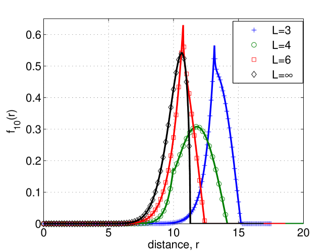
Figure 5: The PDF $f_{10}(\boldsymbol{u};r)$ of the distance to farthest neighbour for a point located at the vertex of the polygon with area $A=100$ and $N=10$ nodes, for triangle ($L=3$), square ($L=4$), hexagon ($L=6$) and disk ($L=\infty$). Solid lines show analytical result using our proposed algorithm and markers provide verification using simulation.

VI Conclusions

In this paper, we have derived the exact cumulative density function of the distance between a randomly located node and any arbitrary reference point inside a regular $L$-sided polygon. We have used it to obtain the closed-form PDF of the Euclidean distance between any arbitrary reference point and its $n$-th neighbour node, when $N$ nodes are uniformly and independently distributed inside a regular $L$-sided polygon. We have provided examples to demonstrate the generality of our proposed framework. Future work can exploit the knowledge of these general distance distributions to model and analyse the wireless network characteristics, such as connectivity [17], interference and outage probability, from the perspective of an arbitrary node located anywhere (i.e. not just the center) in the finite coverage area.

Appendix A Derivatives

By employing the Leibniz integral rule, we can express the derivatives of $B_{\ell}(\boldsymbol{u};r)$ and $C_{\ell}(\boldsymbol{u};r)$, which are required in the evaluation of $\frac{\partial F(\boldsymbol{u};r)}{\partial r}$ in (14), as

$$\frac{\partial B_{\ell}(\boldsymbol{u};r)}{\partial r}\, =\,2r\arccos\left(\frac{p(\boldsymbol{u};S_{\ell})}{r}\right)$$ (24)

$$\frac{\partial C_{\ell}(\boldsymbol{u};r)}{\partial r}\, =\,r\bigg{(}\arccos\left(\frac{p(\boldsymbol{u};S_{\ell})}{r}\right)+\arccos\left(\frac{p(\boldsymbol{u};S_{\ell-1})}{r}\right)-\frac{2\pi}{L}\bigg{)}$$ (25)

References

- [1] S. Srinivasa and M. Haenggi, “Distance distributions in finite uniformly random networks: Theory and applications,” IEEE Trans. Veh. Technol., vol. 59, no. 2, pp. 940–949, Feb. 2010.
- [2] D. Moltchanov, “Distribution of distances in random networks,” Ad Hoc Networks, Mar. 2012. [Online]. Available: http://dx.doi.org/10.1016/j.adhoc.2012.02.005
- [3] P. Fan, G. Li, K. Cai, and K. B. Letaief, “On the geometrical characteristic of wireless ad-hoc networks and its application in network performance analysis,” IEEE Trans. Wireless Commun., vol. 6, no. 4, pp. 1256–1265, Apr. 2007.
- [4] M. Haenggi and R. K. Ganti, Interference in Large Wireless Networks. Now Publishers Inc., 2008.
- [5] J. G. Andrews and S. Webber, Transmission capacity of wireless networks. Now Publishers Inc., 2012.
- [6] F. Fabbri and R. Verdone, “A statistical model for the connectivity of nodes in a multi-sink wireless sensor network over a bounded region,” in Proc. 14th European Wireless Conference, Jun. 2008.
- [7] M. Haenggi, “On distances in uniformly random networks,” IEEE Trans. Inf. Theory, vol. 51, no. 10, pp. 3584–3586, Oct. 2005.
- [8] D. Torrieri and M. C. Valenti, “The outage probability of a finite ad hoc network in Nakagami fading,” IEEE Trans. Commun., 2012 (to appear). [Online]. Available: http://arxiv.org/abs/1207.2711v1
- [9] G. Mao and B. D. O. Anderson, “Towards a better understanding of large-scale network models,” IEEE/ACM Trans. Netw., vol. 20, no. 2, pp. 408–421, Apr. 2012.
- [10] Y. Zhuang and J. Pan, “Random distances associated with equilateral triangles,” ArXiv Technical Report, 2012. [Online]. Available: http://arxiv.org/abs/1207.1511
- [11] A. M. Mathai, An introduction to geometrical probability: distributional aspects with applications. CRC Press, 1999.
- [12] A. Kostin, “Probability distribution of distance between pairs of nearest stations in wireless network,” Electronics Letters, vol. 46, no. 18, pp. 1299–1300, Sep. 2010.
- [13] Y. Zhuang and J. Pan, “Random distances associated with hexagons,” ArXiv Technical Report, 2011. [Online]. Available: http://arxiv.org/abs/1106.2200
- [14] U. Bäsel, “Random chords and point distances in regular polygons,” ArXiv Technical Report, 2012. [Online]. Available: http://arxiv.org/abs/1204.2707
- [15] C. Bettstetter, “On the connectivity of ad hoc networks,” The Computer Journal, vol. 47, no. 4, pp. 432–447, 2004.
- [16] W. L. Martinez and A. R. Martinez, Computational Statistics Handbook with Matlab. Chapman and Hall/CRC, 2001.
- [17] S. Durrani, Z. Khalid, and J. Guo, “A tractable framework for exact probability of node isolation in finite wireless sensor networks,” ArXiv Technical Report, 2012. [Online]. Available: http://arxiv.org/abs/1212.1283