A Mexican Hat with holes: calculating low resolution power spectra from data with gaps

Abstract

A simple method for calculating a low-resolution power spectrum from data with gaps is described. The method is a modification of the $\Delta$-variance method previously described by Stutzki and Ossenkopf. A Mexican Hat filter is used to single out fluctuations at a given spatial scale and the variance of the convolved image is calculated. The gaps in the image, defined by the mask, are corrected for by representing the Mexican Hat filter as a difference between two Gaussian filters with slightly different widths, convolving the image and mask with these filters and dividing the results before calculating the final filtered image. This method cleanly compensates for data gaps even if these have complicated shapes and cover a significant fraction of the data. The method was developed to deal with problematic 2D images, where irregular detector edges and masking of contaminating sources compromise the power spectrum estimates, but it can also be straightforwardly applied to 1D timing analysis or 3D data cubes from numerical simulations.

1 Introduction

The calculation of the Power spectrum through direct Fourier transform of 2D data in astrophysics is often hampered by two problems.

I.

Images may have irregular boundaries or parts of the image are missing. In many cases masks are applied to remove contaminating foreground sources, creating holes in the data that are hard to correct for in Fourier analysis. Such problems arise, for example, when angular fluctuations of a diffuse emission are analyzed and a number of compact sources have to be excised from the image (e.g. Churazov et al., 2012).

II.

Another problem often encountered when dealing with limited data sets is the presence of large scale structures, which are not fully covered by the image. The large scale power can leak into the observable Fourier frequency range, distorting the measured spectrum. This often occurs in 1D timing analysis when the noise process monitored has power on timescales longer than the total length of the time series (e.g. Scott et al., 2003), or in 3D data cubes of hydrodynamical simulations for example, when characterizing the turbulent velocity field in a sub-volume of a larger simulated volume (e.g. Dolag et al., 2006).

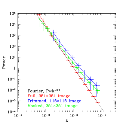
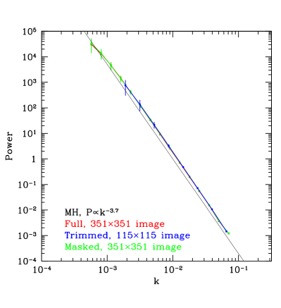
These problems are illustrated in the left panel of Fig.1, which shows the Fourier power density spectrum (PDS) calculated for a 2D image. As input an image with steep PDS $\propto k^{-11/3}$ was used. The red points show the Fourier PDS for the whole image, blue points show the PDS calculated for a section one third of the linear size of the original image and green points show the case when about 25% of the data in the original image are missing and replaced with zero. Changes in the slope and normalization are readily visible for blue and green curves.

A practical way to deal with these problems has been suggested in a series of papers by Stutzki et al. (1998); Bensch et al. (2001); Ossenkopf et al. (2008). Their $\Delta$-variance method preferentially selects fluctuations at a given spatial scale $\sigma$ by convolving an image with two filters - a compact “core” filter and a more extended “annulus”. The core filter has a characteristic size $\sim\sigma$ and both filters are normalized to unity. The difference between the images convolved with these two filters is an image where all fluctuations with sizes much larger or much smaller than $\sigma$ are suppressed. Therefore the variance of the resulting image provides a measure of a typical amplitude of fluctuations of size $\sim\sigma$ in the original image. Introduction of a mask helps to deal with the boundaries or data gaps.

In this paper we discuss a simple method, based on the $\Delta$-variance approach to compute a low resolution power spectrum (strictly speaking the convolution of the true power spectrum with a broad filter) even when a large fraction of the original data is missing. The right panel in Fig. 1 shows power spectra computed with our method for the same images used in the left panel. Compared to the original $\Delta$-variance method, our approach uses a different implementation of the filter, which simplifies the procedure, while cleanly compensating for missing data. We further test this particular implementation for a number of potential applications – e.g. measuring the power spectrum of the surface brightness fluctuations of the X-ray images of galaxy clusters, or characterizing the power spectrum of a turbulent velocity field in simulations.

Many other methods have been devised to deal with data with gaps. Notably, multi-taper analysis techniques have been developed to estimate the power spectra of one-dimensional (Thomson, 1982) and multidimensional (Alfred & Hanssen, 1997) data in Cartesian coordinates and on the sphere (Wieczorek & Simons, 2007). The choice of taper functions is adapted to the type of data to be treated and the number of tapers is chosen to balance the bias and variance in the resulting power spectrum. These methods can recover very high resolution power spectra, suppressing the power leakage produced by the finite data length and are ideally suited to well sampled data where only few or no points are missing. Severe gaps in the data complicate the application of these methods however. Fodor & Stark (1998) deal with large gaps by calculating separate power spectra for each segment and averaging together the results, which is not easily applicable to data sets with varying data and gap lengths or data in more than 1D. Fodor & Stark (2000) uses multi-tapering methods to compute the power spectrum of complete data sets with few small gaps, which requires the calculation of optimized taper functions for the precise structure of gaps in the data. Although this method does a very good job at recovering the power spectral shape, it requires long and complex calculations which are not directly transferable between data sets with different sampling patterns and was only tested for cases where gaps cover a small fraction (e.g. 5%) of the data.

The method we discuss in this paper is simple, robust and computationally fast. It has no tuning parameters and the interpretation of the resulting power spectrum is straightforward. Most importantly, it can be applied without modifications to the data severely affected by gaps of different sizes. The trade-off is its low spectral resolution, so it is useful for cases when the underlying power spectrum is a smooth function of a wavenumber/frequency. Possible applications in astrophysics include aperiodic variability patterns normally found in AGN light curves; analysis of fluctuations in 2D images, e.g. maps of molecular lines, X-ray images, Faraday Rotation Measure maps defined in irregularly shaped regions; characterization of 3D density or velocity fields in numerical simulations. All these cases are often affected to a varying degree by gaps in the data. These gaps arise mainly due to time constraints in the observations in time series, co-adding of several 2D images with different orientations and excision of contaminating sources and limited computational volumes in 3D simulations.

We demonstrate that for data sets of sufficiently large dynamic range the proposed method recovers well the overall shape and normalization of the spectrum even when gaps occupy large fraction of the data set.

In terms of uncertainties in the power spectrum estimation at a given frequency, the method is analogous to the regular Fourier power spectrum, for data sets without gaps, provided that similar binning of the Fourier powers is made in the frequency space.

In the following section we will describe the method (Sec. 2) and demonstrate its ability to recover the original power spectrum from simulated 2D images with gaps in Sec. 3. We also apply the method in spherical coordinates and use it to evaluate the power spectrum for a characteristic case of CMB data analysis in Sec. 3.2. We explore the properties and applications of the method to 3D data cubes in Sec. 4 and 1D time series in Sec. 5. Expected scatter and errors are discussed in Sec. 6 and we summarize our conclusions in Sec. 7.

Figure 1: Left: Fourier power density spectrum (PDS) calculated for a 2D image. As input a $351\times 351$ pixel image with steep PDS ($\propto k^{-11/3}$) was used (shown by the black line). The spectra were obtained by averaging the power spectra, recovered from 50 random realizations of images with the same power spectrum. The errorbars were estimated from the scatter between recovered PDS. The red points show the Fourier PDS for the whole image, blue points show the PDS calculated for a small section ($115\times 115$ pixel) of the original image and green points show the case when about 25% of the data in the original $351\times 351$ pixel image are missing and replaced with zero. Clearly both the normalization and the shape of the PDS are modified when parts of the data are missing or significant power is present on spatial scales larger than the size of the image (case of image subsection). Right: Power estimated using the Mexican Hat filter, corrected for the gaps in the data. The same set of data is used as in the left panel. Clearly the result is insensitive to the presence of the data gaps. There is a weak bias in the normalization, which is discussed in the text and in the Appendix B.

2 Method

We consider an isotropic homogeneous random field, so that it can be characterized by a power spectrum $P(k)$, where $k$ is a scalar. Instead of calculating the “true” power spectrum $P(k)$, where $k$ is the wave number, we want to evaluate the amplitude of fluctuations for a broad interval of wave numbers $\Delta k\sim k$. We allow for gaps in the data and want to recover the correct shape and normalization of the power spectrum, provided that $P(k)$ does not contain sharp features.

The method consists of few simple steps for any given spatial scale $\sigma$:

(i)

the original image is convolved with two filters (e.g. Gaussian) having different smoothing lengths $\sigma_{1}=\sigma/\sqrt{1+\epsilon}$ and $\sigma_{2}=\sigma\sqrt{1+\epsilon}$, where $\epsilon\ll 1$.

(ii)

convolved images are corrected for the data gaps (see §2.2).

(iii)

the difference of two images is calculated. This difference image is dominated by fluctuations at scales $\sim\sigma$.

(iv)

The variance of the resulting image is calculated and re-casted into an estimate of the power.

The variance values are collected as a function of length scale or, correspondingly, wave number $k_{r}\propto 1/\sigma$ to produce the power spectrum $\tilde{P}(k_{r})$. The tilde is added to distinguish the result from the true power spectrum.

We first consider the case of data without gaps (§2.1, steps i,iii and iv) and then discuss the procedure of correcting for gaps (§2.2) using a Mexican Hat filter as an example.

2.1 Data without gaps

To isolate structures of a characteristic length-scale, we first smooth the image $I$ with two Gaussian filters (for simplicity we consider 1D case):

$$G_{\sigma}(x)=\frac{1}{(2\pi\sigma^{2})^{1/2}}e^{-\frac{x^{2}}{2\sigma^{2}}}$$ (1)

of slightly different widths $\sigma_{1}=\sigma/\sqrt{1+\epsilon}$ and $\sigma_{2}=\sigma\sqrt{1+\epsilon}$, where $\epsilon\ll 1$. The top panel in Fig. 2 shows an example of two such Gaussian filters, normalized to unity, together with their difference. For clarity only, in the Figure we use $\epsilon\sim 0.25$. After convolving the image with each of these filters, both resulting images $I_{1}$ and $I_{2}$ will retain structures larger than $\sigma$ and lose structures smaller than $\sigma$ so the difference image $\displaystyle I_{1}-I_{2}$ will predominantly contain structures with the characteristic scales $\sim\sigma$.

For $\epsilon\rightarrow 0$ the resulting filter

$$F(x)=G_{\sigma_{1}}(x)-G_{\sigma_{2}}(x)\propto\frac{\partial G_{\sigma}(x)}{\partial\sigma}(\sigma_{2}-\sigma_{1})\propto$$

$$\propto\epsilon\left[1-\frac{x^{2}}{\sigma^{2}}\right]e^{-\frac{x^{2}}{2\sigma^{2}}},$$ (2)

which is the familiar Mexican Hat filter. Obviously the shape of the filter does not depend on $\epsilon$ in the limit of $\epsilon\rightarrow 0$. In practice we use $\epsilon=10^{-3}$.

Figure 2: Top panel: 2 Gaussians of $\sigma\sim 1$ used for filtering (red, blue) and their difference (black). Bottom panel: Fourier transforms of the Gaussian functions shown above (red, blue), their difference (black) and the difference squared, amplified for clarity (magenta). The magenta curve is the filter effectively applied on the power spectrum of the image treated, therefore the variance of the filtered image is normalized by the area under this curve. The transmitted power peaks at $k=0.225/\sigma$.

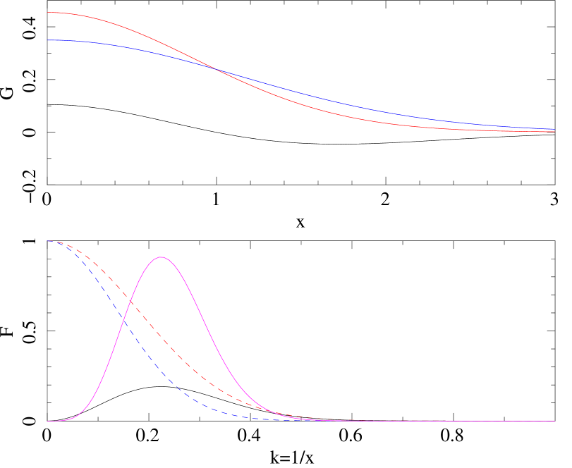
In terms of power spectra, the above procedure is equivalent to multiplying the original power spectrum of the data by the power spectrum of the filter, shown in the bottom panel of Fig. 2. This panel shows the Fourier transforms of the two Gaussian filters, which are of course also Gaussian, and their difference. The square of the difference, is the filter power spectrum. As shown in Appendix A, the peak of the filter power is at $k_{r}=0.225/\sigma$ and its width is $\sim 1.155~{}k_{r}$, independent of $\epsilon$, as long as $\epsilon\ll 1$. Here and below we adopt the relation between the spatial scale $x$ and a wavenumber $k$ in a form $k=1/x$ without a factor $2\pi$. The resulting filter is relatively broad and it cannot be made narrower by using smaller values of $\epsilon$. This has the implication that sharp features in the power spectrum will be smeared out, so our aim is to recover the broad band shape and normalization of the power spectrum but not narrow features. The choice of the Gaussian filters is twofold. Firstly, they provide a good balance in terms of the width in real and frequency space. The width in the real space is important when gaps or edges are present in the data (see next Section). A small width implies that the region affected by a given gap does not extend over the whole image. Secondly, the use of Gaussian filter is computationally convenient, since n-dimensional convolution with a Gaussian in a real space can be easily factorized into 1D convolutions in each dimension.

Figure 3: Top row: simulated image with power law shaped PDS, each subsequent panel shows the result of filtering the image at a different spatial scale $k$ as described in the text, from left to right: $k^{-1}/L=0.6,0.08$ and $0.02$, where $L$ is the size of the image. Bottom row: original image multiplied by the mask, i.e. $I\times M$. Each subsequent panel shows filtered images calculated from the same simulated masked image after application of eq. 8 and multiplication by the original mask, i.e. $I_{c}(k_{r})\times M$. No spurious peaks or dips are produced around the masked regions or near image edges. These parts of the filtered images where $M=1$ are used to calculate the variance for a given $k_{r}$.

Thus the difference between two convolved images, which we denote as $I(k_{r})$ is

$$I(k_{r})=I_{1}-I_{2}\equiv G_{\sigma_{1}}*I-G_{\sigma_{2}}*I\equiv F*I,$$ (3)

can be used to calculate the variance at scales $\displaystyle\sim 1/k_{r}$ and evaluate $\tilde{P}(k_{r})$ using a simple relation for the normalization (see Appendix A).

2.2 Data with gaps

We now consider the image with gaps and introduce a mask $M$ such that

$$M=\left\{\begin{array}[]{ll}1&{\rm where~{}}I{\rm~{}is~{}defined}\\ 0&{\rm where~{}}I{\rm~{}is~{}undefined}\\ \end{array}\right.$$ (6)

Here “undefined” refers not only to gaps, but also to areas outside the image boundaries. Essentially for an $n$-dimensional image we treat the whole $n$-dimensional space outside the image boundaries as a data gap. The image $I$ is also set to zero in the gaps and outside image boundaries. Thus, one can write $I=M\times I_{0}$, where $I_{0}$ is the true image without gaps, defined over the whole $n$-dimensional space.

Direct application of the filter $F$ described by eq. 2 to the image $I$ with gaps will produce many spurious structures, which are difficult to correct for. However one can use the fact that the $I(k_{r})$ image can be represented as the difference of two smoothed images. Consider, for instance, $\displaystyle I_{1}=G_{\sigma_{1}}*I$. Convolving the image with gaps with a Gaussian will still produce spurious features, but their amplitude can be drastically reduced by dividing $I_{1}$ by the mask $M$, convolved with the same Gaussian, to produce a corrected image $\displaystyle I_{1,c}$:

$$I_{1,c}=\frac{I_{1}}{M_{1}}=\frac{G_{\sigma_{1}}*(M\times I_{0})}{G_{\sigma_{1}}*M}.$$ (7)

Note, that we make the convolution in the infinite $n$-dimensional space without assumption of the image periodicity outside the image boundaries. Intuitively the effect of the division by the convolved mask is clear: the amplitude of $I_{1}=G_{\sigma_{1}}*I=G_{\sigma_{1}}*(M\times I_{0})$ is going to be lower close to the gaps or close to image boundaries. The convolved mask $M_{1}=G_{\sigma_{1}}*M$ largely shares these properties and the ratio $\frac{I_{1}}{M_{1}}$ will lack an obvious trend of the amplitude decrease near the gaps. The same argument applies to $\displaystyle I_{2,c}=\frac{I_{2}}{M_{2}}$. Finally

$$I_{c}(k_{r})=(I_{1,c}-I_{2,c})\times M=\left(\frac{G_{\sigma_{1}}*I}{G_{\sigma_{1}}*M}-\frac{G_{\sigma_{2}}*I}{G_{\sigma_{2}}*M}\right)\times M.$$ (8)

The final step of the variance calculation is done only for the part of the corrected image $I_{c}(k_{r})$ where the mask $M=1$ (see Appendix A). In summary, the biases introduced by the shape of the image boundaries and holes in the mask are corrected for by subjecting the mask to the same smoothing procedure and then dividing the smoothed image by the smoothed mask. Therefore, the flux lost by smearing the image out of the mask boundaries is compensated by an equal loss of mask area around the edges. When approaching a gap, the convolved mask $G_{\sigma_{1}}*M$ decreases smoothly from a value of 1 before the gap to 0 well into the gap, provided that the gap is larger than the filter size. Therefore the convolved mask typically has a value of order 0.5 or larger at the edge of the original gap. Since only unmasked parts of the image are used for the variance calculations, points where the denominators in Eq. 8 vanish are automatically discarded.

Our approach is analogous to the $\Delta$-variance method of Stutzki et al. (1998); Bensch et al. (2001) and Ossenkopf et al. (2008). In particular, one of the suggested forms of the filters in Ossenkopf et al. (2008) (see their equation 11) leads to a convolution of an image with a Mexican Hat filter, in the limit of their parameter $v\rightarrow 1$. In other words the difference between filters is the same as used here. However the individual filters are different. Ossenkopf et al. (2008) use a Gaussian as a “core” filter and a ring-like shape function produced by a linear combination of two Gaussians, as a “annulus” filter. In our implementation of the Mexican Hat filter the role of the core and annulus filters (see Stutzki et al. 1998; Ossenkopf et al. 2008 for definitions) is played by two Gaussians with slightly different widths. Far from image gaps and boundaries only the difference between the core and annulus filters matters. But in the presence of gaps or boundaries the functional forms of both filter starts to be important. Representing the Mexican Hat as a difference between two Gaussians simplifies the whole procedure when correcting for the missing data and ensures that the effect of gaps is almost identical for $I_{1,c}$ and $I_{2,c}$.

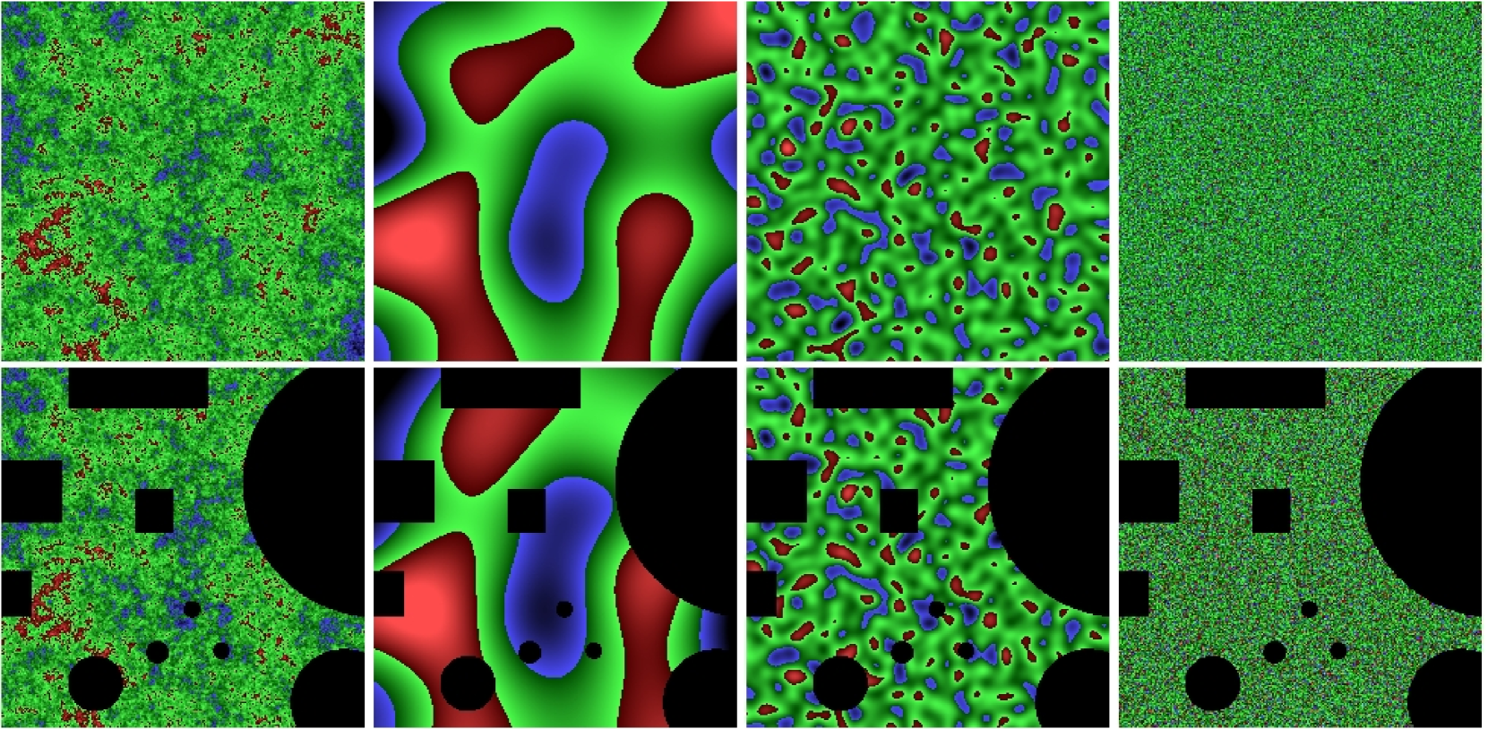
Figure 3 shows a simulated image with an isotropic power law power spectrum of slope $\alpha=-2$. The top row in this figure shows the image decomposition into components of different spatial scales. The bottom row shows the same simulated image to which an arbitrary mask is applied (left). Other images in the bottom row show the decomposition performed on the masked image. Clearly, the method is quite insensitive to the presence of the mask, as seen in Fig. 3. Indeed, the fluctuations on different spatial scales can be recovered in the masked image without introducing spurious structures near the edges or gaps.

3 Test on simulated images

To test the ability of the method to recover the original power spectrum of an image, we generated a set of 2D Gaussian random fields. We simulate the effect of irregular edge shapes and excision of contaminating sources by masking out regions with different shapes and size scales. The mask in Fig. 3 is typical for wide field images when different exposures are combined and contaminating sources are excluded, creating irregular edges and holes in the mosaiced image. For the tests below we use more complicated masks, shown in Fig. 4 to verify the performance of the method in more extreme cases. The tests have also been run using the simple mask shown in Fig. 3, recovering the input power spectra at least as accurately.

Figure 4: Mask 1 (left) and mask 2 (right) applied to simulated 2D images before computing their $\tilde{P}(k_{r})$ spectra. The black areas represent the discarded parts of the input images. Data gaps in real astronomical images are usually less extreme, compared to mask 2. We use this extreme example to test the ability of the method to recover the input power spectrum even for images this heavily affected by gaps.

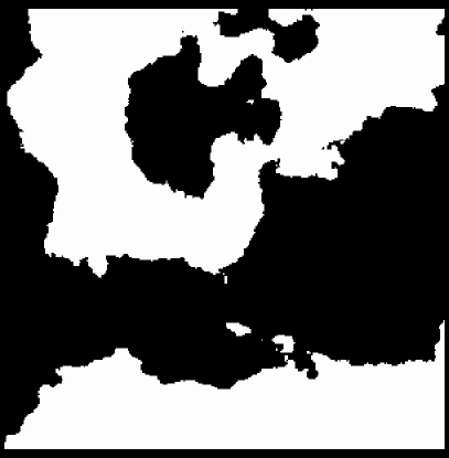
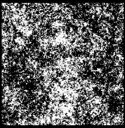
We checked for overall biases in the power spectrum shape and normalization by generating images with randomized phases and amplitudes to simulate a Gaussian field (e.g. Timmer & König, 1995). Images were constructed with power law power spectra of slopes between 0 and –4 and, for each case, 100 realisations were produced and masked by the patterns shown in Fig. 4.

Figure 5 shows the variance of the filtered images as a function of their characteristic filter scale $k_{r}$, for different slopes of the power spectrum. Simulated images had a size of $1024^{2}$ pixels and a central $300^{2}$ pixels section of each image was used to calculate the power spectrum. The $\tilde{P}(k_{r})$ spectra were computed for each simulated image and their average is plotted in Fig. 5 using black dots for the unmasked images, green squares for mask 1 and blue stars for mask 2.

Figure 5: Recovered power spectrum of simulated images. The markers show averaged $\tilde{P}(k_{r})$ spectrum over 100 realizations of simulated images. Black dots show the spectrum computed for unmasked images. Green squares and blue stars correspond to images masked using patters 1 and 2 (see Fig. 4). The slopes of the input power spectra are given in each panel. The input spectra are normalized to unity at $k=1$.

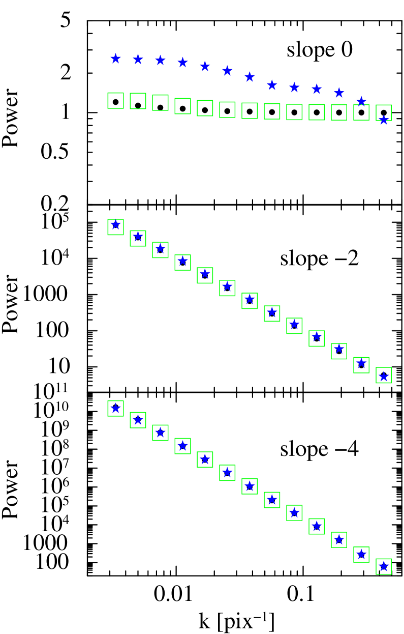
A very small deviation from a perfect power law shape is apparent at the high frequency end of the recovered power spectra even in the unmasked case. This happens because as the filter width approaches the size of the resolution element, the filter is under-sampled and fluctuations at those scales are less accurately recovered. There is a small decrease of power, of not more than 10% of the expected value, at k=0.3 pix ^-1 . Below this frequency the recovered power spectrum is not affected, so if the range of frequencies covered is large, the high frequency part can be discarded and the spectral slope can be accurately measured. Similar effects are seen in 1D and 3D.

The high frequency points in Fig. 5 have the smallest scatter since they are averaged over many Fourier modes. Therefore, the statistical uncertainty, discussed in Sec. 6 is small, and can be smaller than the deviations described above. To avoid assigning too much weight to these points when fitting the measured power spectra, a systematic error of 10% was quadratically added to the estimated statistical uncertainty, associated with each point.

input	No mask		Mask 1		Mask 2		norm
slope	slope	norm	slope	norm	slope	norm	bias
0.0	-0.02	1.00	-0.03	1.03	-0.24	1.33	1
-1.0	-1.00	0.92	-0.99	0.94	-1.04	1.04	0.95
-2.0	-2.00	0.94	-2.00	0.95	-2.01	0.99	1
-3.0	-3.01	1.12	-2.97	1.19	-2.99	1.24	1.25
-4.0	-4.05	1.91	-4.05	1.96	-4.00	2.53	2

Table 1: Results of power law fits to $\tilde{P}(k_{r})$ spectra averaged over 100 realizations of Gaussian random fields in 2D with and without the mask. The input power spectra were normalized to 1 at $k=1$ and have slopes ranging from 0 to -4. For the two groups of columns under the headings Mask 1 and Mask 2, the masks shown in Fig. 4 were applied to the images before calculating $\tilde{P}(k_{r})$. For each case, a recovered power law slope and normalization are given. Deviations in the normalization are largely explained by the normalization bias calculated in Appendix B.

The $\tilde{P}(k_{r})$ spectra were measured for each masked and unmasked simulated image and the average of each set was fit with a power law model. The input and recovered spectral slopes and normalizations, obtained by fitting a power law to the $\tilde{P}(k_{r})$ spectra are given in Table 1.

The spectral power law slopes are recovered with a deviation not larger than 0.24 for any slope probed and not larger than 0.05 for slopes of –1 or steeper. The normalization deviations from unity follow closely the bias expectation given in Appendix B, except for masks similar to Mask 2 and very flat slopes. This mask represents a very extreme case, containing many small scale gaps that distort the power spectrum more than larger gaps as is evident in the top panel in Fig. 5 and in Table 1. For simpler masks and/or steeper power spectra the method recovers the power spectral parameters accurately and the effect of the mask is negligible.

The distortions produced by small gaps covering a large fraction of the image ($>50$%, similar to Mask 2 in Fig. 4) is not easy to predict as they depend on the gap structure. For these cases, when the measured power spectrum slope is flatter than -1, we recommend estimating the distortions through Monte Carlo simulations using known input power spectra and the same gap distribution as in the real data.

The accuracy with which power spectral parameters can be recovered depends on the amount of data available, since this determines the range of scales covered and the density of independent Fourier modes, which affects the errors. As an example we fitted the power spectrum of each individual realization of the images discussed above to measure the scatter in the recovered power law parameters. In these fits, the slope and normalization were fitted simultaneously. The RMS of the recovered parameters are quoted in Table 2. The scatter in the recovered slope and normalization increase for steeper slopes. The scatter is slightly larger for masked images, although there is no significant difference between Mask 1 and Mask 2. Notice that these RMS values characterize the scatter around the biased mean values, similar to those quoted in Table 1.

	No mask		Mask 1		Mask 2
input slope	slope	norm	slope	norm	slope	norm
0.0	0.01	0.02	0.02	0.03	0.02	0.03
-1.0	0.01	0.02	0.02	0.03	0.02	0.03
-2.0	0.02	0.03	0.03	0.02	0.02	0.02
-3.0	0.03	0.05	0.04	0.08	0.03	0.06
-4.0	0.07	0.18	0.07	0.20	0.05	0.20

Table 2: Root-mean-square scatter of recovered power law parameters for sets of 100 simulated images for each spectral slope and mask. The images are (300 pix)² and Masks 1 and 2 are shown in Fig. 4.

3.1 Comparison with the $\Delta$-variance method

As mentioned in §1 and 2.1 the method described above is a further development of the $\Delta$-variance method of Stutzki et al. (1998); Bensch et al. (2001) and Ossenkopf et al. (2008). For the periodic data without gaps both methods produce mathematically equivalent results. We now proceed with a more detailed comparison of the filters performance for non-periodic data with gaps.

The functional form used in Ossenkopf et al. (2008), in the limit of their parameter $v\rightarrow 1$, is as follows :

$$F_{l,core}(x) = \frac{4}{\pi l^{2}}~{}e^{-\frac{x^{2}}{\left(l/2\right)^{2}}}$$

$$F_{l,ann}(x) = \frac{4}{\pi l^{2}}\frac{x^{2}}{\left(l/2\right)^{2}}~{}e^{-\frac{x^{2}}{\left(l/2\right)^{2}}},$$ (9)

where $l$ is the size of the filter. It is obvious that the difference between these two filters is the Mexican Hat filter. However the shape of the second filter $F_{l,\rm ann}(x)$ is very different from the first one $F_{l,\rm core}(x)$. Therefore it is expected that the impact of edges and gaps will be different for the filtered images corrected for these gaps and edges. This is in contrast with the representation of the Mexican Hat filter as the difference between two Gaussians with almost equal width, which guarantees that the gaps have essentially identical impact on both Gaussian convolutions leading to the filtered images.

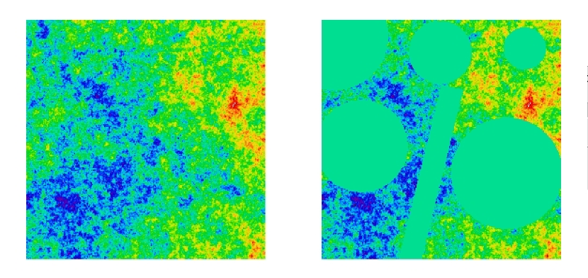
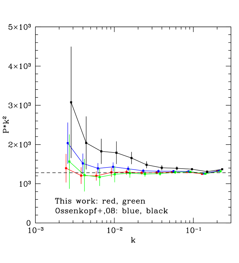
To verify the above conjecture we made a number of test with different power spectra and masks. An example of an image and its masked version is shown in Fig. 6. As before the non-periodic image was obtained by cutting a section of a larger periodic image, in which a random realization of a Gaussian random field with slope -2 was generated. The spectra recovered from the original and masked images for both methods are shown in Fig. 7. The red and green points were obtained using the procedure described in §2.2, for the original and masked cases, respectively. Both for the original and for masked images the spectrum agrees well with the input spectrum, shown by the horizontal dashed line. The spectrum, obtained using Eq. 9 shows larger deviations from the true input spectrum, especially for the masked image, shown in black. Similar results were obtained for other types of masks probed. We therefore conclude that for non-periodic data sets with gaps the filtering based on two nearly identical Gaussians provides more robust and accurate results. We note that the value of $v$ recommended by the authors is $v=1.5$. Repeating the test for this value of $v$ gave similar results to the $v=1$ case and our approach with similar Gaussian still proved more accurate.

Figure 6: Original image with power spectrum with slope -2 (left) and its masked version (right). This non-periodic image was obtained by cutting a small section of a larger image. These images are used to compare the performance of the two filtering methods.

Figure 7: Comparison of the recovered power spectra using the difference between two Gaussian and Eq. 9. The spectra were multiplied by $k^{2}$, so that the input spectrum is flat in this plot (shown by the horizontal dashed line). The spectra were averaged over 10 independent realizations. The red and green points were derived from the original and masked images respectively, using the filter described in this work. The blue and black curves correspond to the original and masked images respectively, processed using the pair of filters from Ossenkopf et al. (2008). For non-periodic data sets and/or for data with gaps the filter based on two nearly identical Gaussians performs better.

3.2 The 2D sphere: application to CMB analysis

The same method can be constructed in spherical coordinates. As an example, in this section we apply the filter formalism to the study of temperature anisotropies of the Cosmic Microwave Background (CMB) radiation. Let $t(\mn@boldsymbol{n})$ be the CMB temperature in the direction $\mn@boldsymbol{n}$. A decomposition of the $t(\mn@boldsymbol{n})$ map on the sphere in a basis of spherical harmonics is,

$$t(\mn@boldsymbol{n})=\sum_{l=2}^{\infty}\sum_{m=-l}^{l}a_{l,m}Y_{l,m}(\mn@boldsymbol{n}),$$ (10)

where $Y_{l,m}(\mn@boldsymbol{n})$ is the spherical harmonic of order $l,m$ evaluated at the direction $\mn@boldsymbol{n}$ and $a_{l,m}$ are multipole coefficients. We assume that $t(\mn@boldsymbol{n})$ is a Gaussian isotropic and homogeneous random field. The angular power spectrum $C_{l}$ for multiple $l$ can be estimated as

$$C_{l}=\langle|a_{l,m}|^{2}\rangle,$$ (11)

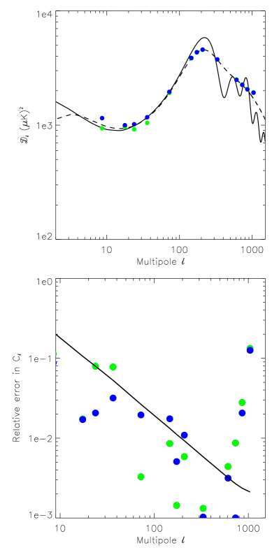
where the averaging is done over $m$. Figure 8, shows the theoretical prediction for the angular power spectrum of the CMB temperature anisotropies for different angular frequencies (or multipoles $l$). The units of the y-axis are ${\cal D}_{l}\equiv l(l+1)C_{l}/(2\pi)$.

Similarly to the Cartesian 2D case described in §2.2 one can define a filter as a difference between two Gaussians defined on a sphere and allow for the data gaps. This yields an image (cf. eq. 28)

$${t}_{\sigma}(\mn@boldsymbol{n})=\left(\frac{G_{\sigma_{1}}*t}{G_{\sigma_{1}}*M}-\frac{G_{\sigma_{2}}*t}{G_{\sigma_{2}}*M}\right)\times M(\mn@boldsymbol{n}),$$ (12)

dominated by a particular angular scale $\sim\sigma$. As before the variance of the resulting image is calculated and divided by the power of the filter. In the multipole space the corresponding filter has the same properties as the 2D filter in Cartesian coordinates, described in the Appendix A (see eq. 25). Namely,

$$\hat{F}_{\sigma}(l)=e^{-l(l+1)\sigma_{1}^{2}/2}-e^{-l(l+1)\sigma_{2}^{2}/2}\approx$$ (13)

$$\approx\epsilon l(l+1)\sigma^{2}e^{-l(l+1)\sigma^{2}/2},$$ (14)

where $\sigma_{1}=\sigma/\sqrt{1+\epsilon}$, $\sigma_{2}=\sigma\sqrt{1+\epsilon}$ and $\epsilon\ll 1$.

The expected shape of the power spectrum can be calculated as:

$$\tilde{C}_{l_{r}}=\frac{\sum_{l}C_{l}|\hat{F}_{\sigma}(l)|^{2}(2l+1)}{\sum_{l}|\hat{F}_{\sigma}(l)|^{2}(2l+1)},$$ (15)

where $l_{r}$ is defined as the multipole where $|\hat{F}_{\sigma}(l)|^{2}$ reaches its maximum. The corresponding angular power spectrum $\tilde{C}_{l_{r}}$ is shown in Figure 8 with the dashed line. Clearly, the filtering procedure smears out small scale features, but recovers the overall shape and normalization of the power spectrum. This smoothed power spectrum is what we want to recover from the data using the proposed method.

In real data, the estimation of the angular power spectrum must deal with the pixelized data and with the presence of the Milky Way and other contaminants that make necessary the exclusion of some pixels on the sky map. We used HEALPix to deal with the pixelized maps. The power spectrum is evaluated from the variance of the filtered images $\displaystyle\langle{t}^{2}_{\sigma}\rangle$ as

$$\tilde{C}_{l_{r}}=\frac{\langle{t}^{2}_{\sigma}\rangle}{\sum_{l}\frac{2l+1}{4\pi}|\hat{F}_{\sigma}(l)|^{2}|W_{l,px}|^{2}},$$ (16)

where $W_{l,px}$ is the window multipole function for the HEALPix pixel.

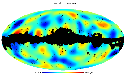
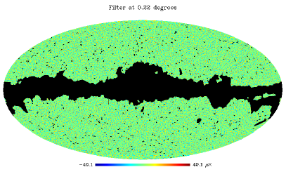
The presence of a mask usually biases the estimation of the power spectrum multipoles ($C_{l}$-s) and, at the same time, it couples these otherwise independent quantities. To test the method we impose a sky mask that covers $\sim$ 24% of the sky, including the Galactic plane and the position of bright radio sources. We also consider two different hemispheres of data separately, defined by an equatorial plane perpendicular to the direction (l,b)=(0°, 45°) in Galactic coordinates. Therefore, each hemisphere analyzes roughly 38% of the sky. We apply filters, of width of 0.1°, 0.12°, 0.22°, 0.35°,0.42°, 0.5°, 1°, 2°, 3°, 4°, 8°, 10°and 20°. An example of a masked CMB realization, filtered at two different scales is shown in Fig. 9. When applying our thirteen different filters in the two masked hemispheres, we obtain $\tilde{C}_{l_{r}}$ for each hemisphere, displayed by the filled green and blue circles, in Fig. 8. The estimates from the two different hemispheres and for each filter scale $\sigma$ follow closely the theoretical prediction provided by the dashed line.

For a single realization of the sky, the relative scatter of power spectrum estimates with respect to the average value is known to approximately follow the scaling

$$\frac{\Delta\tilde{C}_{l_{r}}}{\tilde{C}_{l_{r}}}=\sqrt{\frac{2}{(2l+1)(\Delta l)f_{\rm sky}}},$$ (17)

which corresponds to the black solid line in the bottom panel of Fig. 8. The symbol $f_{\rm sky}$ denotes the fraction of the sky covered in each hemisphere (around $\sim$36% ), and $\Delta l$ provides the effective width, in multipole space, of each filter. The blue and green circles show that the estimates of the angular power spectrum are scattered around the theoretical expectation by an amount that is not far from the theoretical prediction. This behavior breaks down at smaller angular scales, due to effects related to the finite pixel size, which in this case is slightly below 7 arc minutes.

Figure 8: Input angular band power spectrum (solid line), the result of filtering such power spectrum with scale changing filters (dashed line), and the result of computing the angular power spectrum with 13 different filters in two different hemispheres of a masked single CMB sky realization (green and blue circles). In the bottom panel we show the relative error of the power spectrum estimates with respect to the theoretical prediction (dashed line in top panel). The solid line provides the theoretical expectation, $\sqrt{2/(2l+1)/{\Delta_{l}/f_{\rm sky}}}$ with $f_{\rm sky}=$fraction of the sky not being masked. At $l$ values higher than $\sim 800$ the filter size reaches the pixel scale and the errors detach from the theoretical prediction.

Figure 9: Simulated CMB type maps, masked to remove the Galaxy and foreground point sources, and then filtered at two different angular sales. The maps show no evidence for spurious feature near the edges of the mask.

4 3D data cubes

When analysing data of numerical simulations, e.g. a velocity field in hydrodynamic simulations, one often deals with 3D data cubes. In this section we extend the method on three dimensions and compare our power spectrum results with calculations using the conventional Fourier transform. As before, we generate isotropic Gaussian random fields with a power law power spectrum spectrum, in 3D. In particular we consider a red noise process with slope $-11/3$, corresponding to the 3D Kolmogorov power spectrum, which is often assumed when dealing with the turbulent velocity field.

Figure 10: Power spectra calculated through the variance for boxes of different sizes (same as Fig. 11). Top: initial size of the box; middle and bottom: $1/2$ and $1/4$ of the original size on a side respectively. Red: the mean of 100 cube realization, gray: the range of statistical uncertainties corresponding to 1 $\sigma$ scatter.

Figure 11: Fourier power spectrum calculated for a simulated box of $64^{3}$. The power spectrum was obtained by averaging power spectra calculated for 100 random realizations with the same slope $\alpha=-11/3$. The input power spectrum is shown with the dashed line. Blue, red and green curves show the recovered power spectra from the initial box size ($64^{3}$ cells), and trimmed sections of $1/2$ and $1/4$ of the original size on a side, respectively.

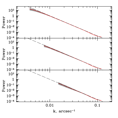
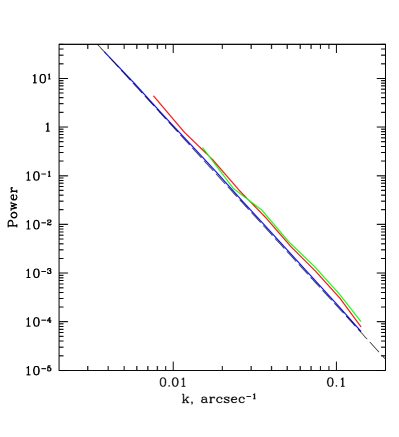
The power spectrum $\tilde{P}(k_{r})$ is calculated analogously to the 2D case, by filtering the cube with 3-dimensional Gaussians. The analysis in Appendix A is directly applicable for $n=3$. As before we assume isotropy in the random field, so we are only interested in the power spectrum as a function of spatial scale.

The first question we address is whether the shape of the red noise is recovered well when the noise extends below the lowest wave numbers set by the size of the cube. To this end we calculate the power spectrum for the full simulated box and also for smaller “trimmed” boxes, which are cut from the original larger cube. The mean of 100 power spectra evaluated through the variance (see §2) for the full box and trimmed sections, 1/2 and 1/4 of the original size on a side, are shown in Fig. 10. The 1$\sigma$ statistical uncertainties for all three cases are shown on Fig. 10 with gray shadows. The mean of 100 cube realisations and their trimmed sections are shown by the red lines on each panel, while the scatter is represented by the gray area. Power spectra calculated through the conventional Fourier transform are shown in Fig. 11. The input power law power spectrum is shown by the dashed black line. Since trimmed cubes are not periodic anymore the power spectrum recovered through Fourier transform is strongly distorted by leakage of power from very low frequencies. However, we see good agreement between the input and recovered power spectra calculated through the variance method. The minor discrepancies are only on the smallest and highest wave numbers.

Both discrepancies are caused by the fact that the value of the variance is a convolution of the true PDS with the filter in frequency space. As a result at low $k$ the power leaks out if the full simulated box is used, the simulated cubes effectively have zero power at frequencies lower then $1/L$. This effect goes away if a subsection of the original cube is used (see also 2D case in Fig. 1).

We now proceed by considering the impact of data gaps on the recovered power spectra. We consider 3D masks covering different fractions of the cube volume. Slices of masks through the box center are shown in Fig 12. The first two masks are generated randomly and the fraction of missing data is 50 per cent in the left panel to 85 per cent in the middle panel. Often, when one deals with simulations of galaxy clusters, large sub-halos or one of the sub-clusters in merging systems are excluded from the analysis. Consequently, we generated a third 3D mask that mimics a situation when large sub-halo is excluded. The slice of this mask is shown on the right panel in Fig.  12.

Figure 12: Slices of masks we applied to the data boxes in our calculations. Slices are through the center of the box. Black: excluded data, $M=0$; white: data used for power spectrum calculations, $M=1$. Left and middle panels: masks are generated with random gaps. The fraction of discarded data is 50 and 85 per cent. Right panel: mask mimics the case of excluded sub-halo.

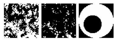
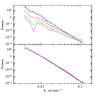
Figure 13 shows the power spectrum of the data with gaps calculated through the conventional Fourier transform and with the variance method. Clearly, the direct Fourier method should not be used for data with gaps. The increase of the gaps fraction leads to the leakage of power causing the flattening of the spectrum and the decrease of its normalization. At the same time the power spectra calculated through the variance are perfectly recovered, with only minor changes on small and large wave numbers even in case when 85 per cent of the data are in gaps.

Figure 13: Power spectra calculated for data with gaps (one realization). Top: Fourier method, bottom: variance method. Dashed curves show initial power spectrum. Blue: 50 per cent of data is discarded, see the left panel in Fig. 12; red: 85 per cent of data is excluded, the middle panel in Fig. 12; green: large sub-volume of the box is excluded, see the right panel in Fig. 12. Fourier method changes the slope and normalization of the recovered power spectrum, while the variance method recovers power spectrum without distortions on a large range of wavenumbers.

5 1D: Timing analysis

A possible 1D application of the method can be found in the study of light curves of variable objects. The method is of course not suitable for the search of periodicities, but can be useful for studies of aperiodic variability, when the broad band shape of the power spectrum is of interest.

The top panel in Fig. 14 shows a simulated light curve typical for long term X-ray monitoring of an Active Galactic Nucleus (AGN) (e.g. Uttley et al., 2002; Markowitz et al., 2003). The power spectra of these light curves is normally modeled as a single or broken power law, where the slopes and/or break frequencies are of interest (e.g. McHardy et al., 2006; Papadakis et al., 2009). These light curves often have yearly gaps due to visibility constraints and different variability time-scales are covered by varying the sampling rate. The window function produced by these gaps causes spurious features in the power spectrum and different approaches have to be used to remove these features from the Fourier transform of the light curve (e.g. Uttley et al., 2002; Markowitz, 2010; Emmanoulopoulos et al., 2010; Kastendieck et al., 2011).

Figure 14: Top: Simulated light curve, typical of AGN long term X-ray monitoring, with varying sampling frequency and containing yearly gaps. Bottom: The sampling rate varies with time, here the time difference between consecutive observations is plotted as a function of time, except for the largest gap, after the short, high cadence monitoring.

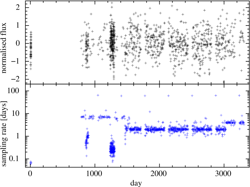
The case of AGN light curves is essentially different from images and simulated data cubes since normally the light curves are not sampled continuously over a regular grid, but consist of snapshot observations on irregularly spaced time intervals. Long term AGN light curves, as described above, suffer strongly from this effect, since the timescale coverage is optimized by combining epochs of very different sampling rates as shown in the bottom panel of Fig. 14. For our example, frequencies from $3\times 10^{-9}$ to $3\times 10^{-5}$ Hz are probed using only 1100 light curve points. If it was evenly sampled, this range would require 20.000 points. This uneven sampling does not pose a problem to the variance calculation, since the filter convolution can be performed over uneven grids. In this case, the mask is simply the same time series, with all flux values replaced by 1. Figure 15 shows the filtered light curves on different timescales produced by this approach, gaps in the time series and varying sampling rates do not prevent a clean filtering of the fluctuations.

Figure 15: Result of the filtering routine on the light curve shown in Fig. 14. Gaps in the light curve do not affect the filtering process. Short timescales are only probed by higher cadence light curve segments. This is achieved by discarding data points that have less then 6 neighbors within a time space of $4\sigma$ for each value of the filter width $\sigma$ while calculating the convolution. The panel on the left shows light curves filtered on timescales of 3300, 1100, 366, 121, 13.5, 1.5 and 0.5 days. The panel in the right shows a zoom to the most intensive monitoring section, at the beginning of the light curve, for filter timescales of 13.5, 4.5, 1.5 and 0.5 days, from top to bottom.

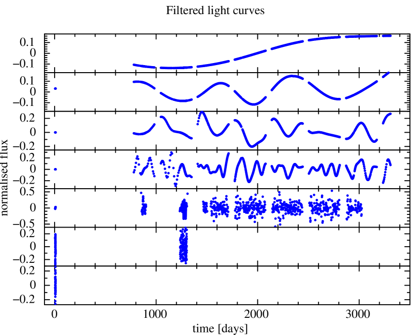
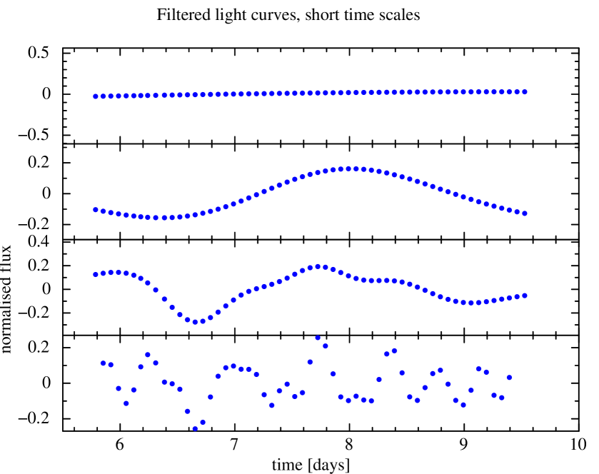
In Figure 15 we have only plotted the useful part of each filtered light curve, these sections are selected to reduce the effect of aliasing, which is potentially a larger problem for light curves than for images. In the case of isotropic fluctuations in images, fluctuations on length scales shorter than the pixel size are averaged out. In the case of light curves, unless they are continuously exposed, variability on timescales shorter than the sampling interval adds to that of the longer fluctuations. This effect aliases power into lower frequency bands and distorts the measured power spectrum.

Aliasing can be diminished by demanding a minimum number of exposures within the convolution Gaussian around a given lightcurve point for this point to count towards the variance calculation. In other words, if a point in the light curve has no neighbors closer than $4\sigma$, for a given filter width $\sigma$, then it cannot provide information on the corresponding frequency $k_{r}$. Therefore, although the point can participate in the convolution of the light curve, it should not be counted in the variance for that frequency. The procedure applied on the simulated light curve counts the number of neighbors for each point in the light curve while making the convolution and later discards points that have less than 6 neighbors for a given filter width, producing the filtered lightcurves in Figure 15. Therefore, the shorter timescales are only probed by the more intensively sampled sections.

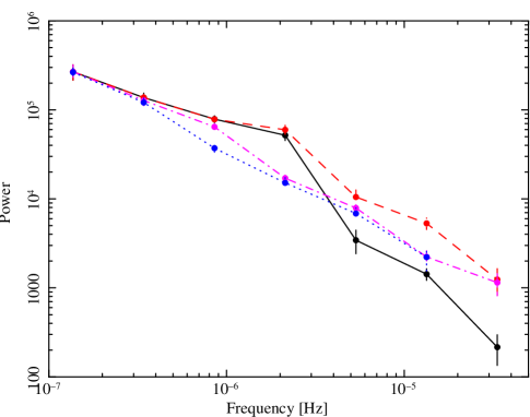
We tested the recovery of the input power spectra for unevenly sampled light curves for different minimum numbers of neighbors within $4\sigma$ of each point. Figure 16 shows an example of these tests, for simulated light curves of power law slope -1. Each power spectrum is the average of 100 simulations, to average out the fluctuations between different realizations. In the Figure, the black solid line represents the power spectrum with no minimum number of neighbors required, so that all light curve points count towards all frequency bins. The peak in the middle is the effect of aliasing and the drop at high frequencies is the result of counting many isolated points in the variance, since these have all the same value they reduce the variance artificially. The red dashed line uses at least two neighbors and already corrects this last problem, while the aliasing is not resolved. Requiring 6 neighbors (pink dot-dashed line) already solves a large part of both problems, while requiring 10 neighbors (blue dotted line) produces a power spectrum quite close to the input power law. Using more neighbors does not improve the recovered power spectrum but it reduces the probed frequency range, since at high frequencies the sampling rate itself limits the number of possible neighbors.

Figure 16: The minimum number of neighbor points required to count a point in the variance calculation affects the shape of the resulting power spectrum. The power spectra above are each an average of 100 realizations, requiring 0 neighbors (solid, black), two neighbors (red, dashed), six neighbors (pink , dot-dashed) and ten neighbors (blue, dotted). Requiring more than 10 neighbors does not improve the recovered power spectrum and reduces the sampled frequency range as explained in the text. Error bars denote the RMS scatter in each set of simulations.

Finally, the entire power spectrum of the full range of frequencies covered by the light curve in Fig. 14 can be computed directly. Figure 17 shows the result of applying the filter formalism using a minimum of 6 neighbors to simulated light curves with the same sampling pattern and a bending power law power spectrum. For this Figure, 100 random realizations were averaged together. At low frequencies the flat input slope and extreme mask produces the slope bias expected from the results in Table 1 while the high frequency normalization is biased upwards by a factor of 1.3, as expected from Appendix B. The approximate slopes, break and normalization of the input power spectrum, shown by the solid line, are clearly recovered.

Figure 17: Power spectrum of the simulated light curve with the same sampling as in in Fig. 14 with a flat input power spectrum which bends to a power law slope of –2 at a frequency $10^{-6}$ Hz. The black symbols correspond to $\tilde{P}(k_{r})$ averaged over 100 realizations of the light curve. Error bars denote the RMS scatter in each set of simulations.

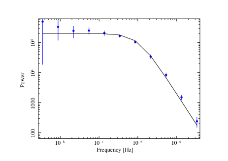
For light curves similar to the one shown in Fig. 14 the power spectrum is usually estimated through Monte Carlo simulations of sample light curves with given power spectrum parameters, attempting to recover only power law slopes, breaks and normalizations.

The simplicity of the variance method is that it can be applied directly on the full light curve, regardless of the gap and sampling distributions and reproduce the overall shape with approximately correct normalization of the power spectrum. This will be particularly useful for large samples of AGN light curves from large-area repeated surveys, where estimation of aliasing and red noise leak for each particular AGN becomes impractical. For comparison, power spectrum fitting of the light curve in Fig. 14 using PSRESP (Uttley et al., 2002) takes several hours whereas $\tilde{P}(k_{r})$ and its error estimate can be obtained in a few seconds on the same computer and both methods recover the spectrum with similar accuracy.

6 Error estimation

As with other methods, it is possible to predict the uncertainty of the power estimates by assuming certain properties of the underlying variability process. In this case we will assume that the data being treated correspond to a Gaussian field, so that independent points in the power spectrum are distributed around their mean values as a $\chi^{2}$ distribution with two degrees of freedom, with standard deviation equal to the mean. This means that the uncertainty of the power for each individual Fourier mode is equal to the power itself. Therefore, to calculate the expected uncertainty in a frequency bin, it is only necessary to combine quadratically the power at the frequencies that fall within the bin.

The effect of the filter in frequency domain is to make a weighted average of the power spectrum estimates within the width of the filter. Therefore, the expected uncertainty, $E$, of $\tilde{P}(k_{r})$ can be calculated as a weighted mean of the $P(k)$ values that fall under the frequency filter, where the values are combined quadratically.

Independent Fourier modes in each dimension are separated in frequency by $1/N_{i}$ where $N_{i}$ is number of pixels in dimension $i$. This spacing needs to be taken into account when calculating the uncertainty in order to include the correct number of power estimates under the filter. In the case of isotropic fluctuations in $n$ dimensions, where we only calculate the power as a function of $k=\sqrt{\sum_{i=1}^{n}(j_{i}/N_{i})^{2}}$, different groups of indices producing the same value of $k$ are averaged together and this should also be considered in the uncertainty calculation.

The correct density of Fourier modes is easily obtained by summing over all the independent modes, or equivalently over half the data points, i.e. over points $j$, from 1 to $N_{1}/2$ in the first dimension and from 1 to $N_{i}$ in all the following dimensions as

$$E(k_{r})=\frac{\sqrt{\sum_{j=1}^{N/2}(P(j/N)\hat{F}^{2}_{k_{r}}(j/N))^{2}}}{\sum_{j=1}^{N/2}\hat{F}^{2}_{k_{r}}(j/N)}.$$ (18)

for 1 dimension and

$$E(k_{r})=\frac{\sqrt{\sum_{j=1}^{N_{1}/2}\sum_{l=1}^{N_{2}}(P(k)\hat{F}^{2}_{k_{r}}(k))^{2}}}{\sum_{j=1}^{N_{1}/2}\sum_{l=1}^{N_{2}}\hat{F}^{2}_{k_{r}}(k)}.$$ (19)

for 2 dimensions. For larger $n$ the formula is similar.

The filter $\hat{F}_{k_{r}}(k)$ is centered on $k_{r}$ in frequency domain and is given in equation A6. Clearly for larger data sets (larger $N_{i}$), the independent modes are spaced more closely in frequency so more power spectrum points are averaged together under the same filter width and the uncertainty decreases accordingly as $1/\sqrt{\Pi_{i=1}^{n}N_{i}}$. Since the number of Fourier modes within the filter width grows linearly with increasing frequency in each dimension, the expected error spectrum is steeper than the powerlaw power spectrum by 0.5 in 1-D, by 1 in 2-D and by 1.5 in 3-D. As shown in the next section, this prediction is well matched by the data.

The expected error can be calculated in one pass through the data points per frequency $k_{r}$, so it does not imply a significant computational effort.

The assumption of a Gaussian field implies that each independent frequency will have its power distributed as a $\chi^{2}$ distribution with two degrees of freedom but the average over many such points will lead to a Gaussian distribution. For low frequencies the number of Fourier modes within the filter is small, so the distribution of powers deviates noticeably from Gaussian. However, since the filter is broad in frequency, in 1D $k_{r}=4/T$ already contains enough points to produce an approximately symmetric distribution of measured power. In 2D and 3D cases the symmetry is achieved at even lower frequencies since the number of Fourier modes within the filter grows as $k^{n}$.

The values of $P(k)$ in the error formula can be estimated by interpolating between measurements of $\tilde{P}(k_{r})$, given that the true underlying form is not known a priori. Using the measured power spectrum in the error formula automatically takes into account the normalization bias and any other distortions, so that the resulting errors always represent the statistical uncertainty around the measured values. If the spectrum is finally rescaled by the normalization bias, the errors should be rescaled accordingly.

6.1 Comparing expected error with measured scatter

The error formula predicts the scatter of $\tilde{P}(k_{r})$ measurements around the underlying power spectrum for a Gaussian noise process. We tested the accuracy of this approach by comparing directly the predicted error to the RMS scatter in 100 realizations of a noise process. Figure 18 shows this comparison of measured scatter in markers and predicted errors in lines, both relative to the measured power spectrum. Solid lines and nearby markers correspond to 1D time series without gaps with input power spectra slopes of -1 and -2 (the power spectra themselves are not shown here). There is a very good agreement between the measured RMS spread and the estimated uncertainty $E$ in the case of continuous data sets. The error estimate described in this section is equivalent to the expected scatter from Fourier analysis in the case of continuous data sets. The analysis above shows that the scatter around the mean power in binned Fourier transforms and in $\tilde{P}(k_{r})$ spectra are identical, so both methods are equivalent when measuring low resolution power spectra of data without gaps.

6.2 Effect of gaps on the error estimate

Evidently, gaps in the data will reduce the number of available independent points and so the uncertainty in the power spectrum measurement should increase. As a first step to model this effect we scale $E$ by the number of points actually available in the data ($N_{a}$) compared to the total number of points if there were no gaps $N$: $E^{\prime}=E\times\sqrt{N/N_{a}}$.

As a further refinement, it is convenient to count the number of available points as a function of $k_{r}$, since small gaps do not affect the power estimates at low wavenumbers. This estimate is shown by the dashed lines in Fig. 18. A good match to the measured scatter (markers closest to the dashed lines) was obtained when points in gaps were discounted only if the gap was longer than 10% of the filter spatial scale ($1/k_{r}$). The errors and scatter measurements correspond to the same sets of simulated light curves discussed above, this time masked by gaps of random lengths so that 85% of the points were discarded. The uncertainty for each slope increases and the increase is larger at small spatial scales, which are affected by more gaps. In any case, the increase in uncertainty for any length scale is between $E$ and $E\times\sqrt{N/N_{a}}$, so that for a small fraction of missing points the dependence of the error increase on $k_{r}$ can be neglected.

In the case of light curves with uneven sampling and very different sampling rates it is more convenient to scale the error by the lengths of useful data stretches to the total length. As before, useful light curve stretches can be selected for each frequency $k_{r}$ by requiring a minimum number of neighbors for useful data points. All useful segments are added to produce $T_{u}(k_{r})$ and the error is scaled as $E\times\sqrt{T_{\rm tot}/T_{u}}$, where $T_{\rm tot}$ is the total length, used to calculate the frequency spacing.

Figure 18: Comparison of predicted relative error (lines) with measured RMS scatter (markers), for sets of 100 $\tilde{P}(k)$ of simulated light curves. The solid lines and corresponding markers are calculated for continuous light curves of 2048 points and power law slopes of –1 (blue lines and markers) and –2 (red lines and markers). The dashed lines and markers show the predicted and measured errors for the same light curves after 85% of the data points have been masked out producing gaps of random length. For this range of slopes at least the analytic prediction of the uncertainty in Eq. 19 works well.

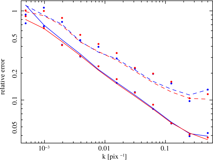
When using these error estimates to fit models to the power spectrum it is necessary to use only independent measurements that, given the mixing effect of the filter, should be separated by at least a factor or 2 in frequency.

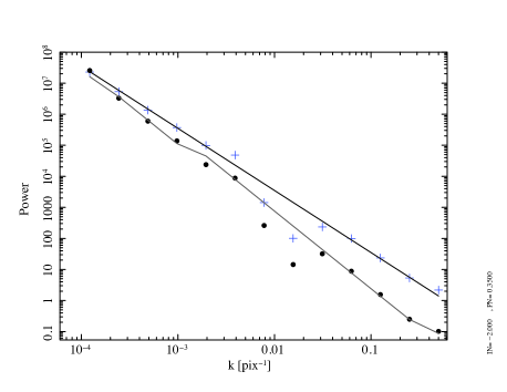
The analytic error estimate was compared to Monte Carlo simulations of Gaussian fields in 1, 2 and 3D, for simple power law or broken power law power spectra of zero or negative slopes. Although this is a limited subset of all possible power spectra it does cover a wide range of astrophysical phenomena of interest. More examples are given in Fig. 19. Here 2D images with broken power law power spectra and affected heavily gaps as shown in mask 2 of Fig. 4 are examined. The decrease in number of points was estimated from gap size distribution in the x direction only to estimate the errors. Since the gap structure is largely isotropic, this simple 1D estimate gave a good approximation, shown by the dashed line, error estimates from RMS scatter of 100 trials is shown in black markers. In the same figure we plot the predicted error and RMS scatter of 100 simulated data cubes with power law slope –11/3, also masking out 50% of the data points. The mask in this case is similar to that shown in Fig. 12, which affects all scales in approximately the same way so the effect of the mask can be estimated simply by rescaling the predicted error by the square root of the ratio of the total number of points to the number of points actually available.

Figure 19: Relative error prediction for 2D (red) and 3D (blue) data. In this example the input power spectrum of the 2D data is a broken power law of low frequency slope –0.5 and high frequency slope –2.5, and for the 3D data is a power law of slope –11/3. The images have been masked out by random sized gaps covering 50% of the image. The predicted errors divided by the average power spectrum are shown by the dashed lines and the measured RMS scatter of the 100 realizations is shown by the blue and red markers. The error formula in Eq. 19 predicts the errors accurately for simple and broken power law spectra in images and data cubes as well.

6.3 Data with periodic gaps

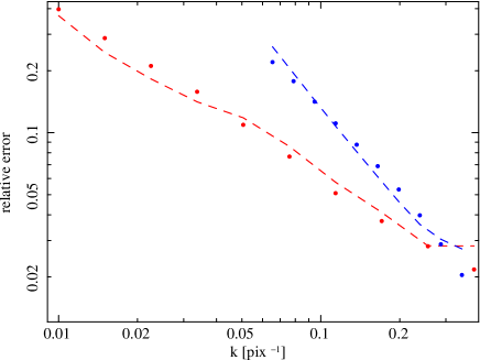
A special case that we considered is largely found in 1-D light curves where observational constraints produce strictly periodic gaps. If the data and gap stretches are of equal length or the data stretch is longer, then the variance method and error estimate can be directly applied. However, if the gaps ($T_{g}$) are longer than the data stretches ($T_{d}$) and the sampling pattern is strictly periodic, then some timescales are effectively not probed by the data and the method cannot be expected to produce reliable power spectral estimates for the corresponding frequencies. Frequencies above $(2\times T_{d})^{-1}$ and below $(4\times(T_{d}+T_{g}))^{-1}$ are properly reproduced and the error estimate applies, as shown with an example in Fig. 20 . The power spectrum of frequencies within this range are not reliable and should be discarded.

Unsurprisingly, it is possible to recover the power spectrum for the timescales that are well sampled, either shorter than each individual data stretch $T_{d}$ or longer than a few times the sampling interval. In cases like this it is common to make separate estimates for the high and low frequency power spectrum, by averaging together individual power spectra from short stretches for the first case and by computing the power spectrum of low resolution light curves, averaging together data over $T_{d}$ and using the sampling interval as time step for the latter. One of the advantages of the variance method is that it can compute reliably the same range of frequencies directly from the complete light curve, without any further manipulation of the data.

Figure 20: Effect of periodic gaps in 1-D data. The above $\tilde{P}(k_{r})$ spectrum is the average of 100 realizations of slope –2 light curves masked by periodic gaps, where every 20 data points are followed by 80 gap points. The RMS spread of the simulations is shown by the black markers and the uncertainty predicted by Eq. 19 is shown by the corresponding black line. The average power spectrum in blue crosses fits well the input power spectrum shown by the top black line and the error estimate works well for frequencies above $(2\times T_{d})^{-1}=0.025$ and below $(4\times(T_{d}+T_{g}))^{-1}=0.0025$, the power spectrum for frequencies in between these values should be discarded.

7 Conclusion

A simple method for estimating a low resolution power spectrum from data with gaps is described. Essentially the variance associated with a given scale is calculated by convolving the image with a Mexican Hat filter. Gaps in the data, described by the mask $M$ are corrected for by representing the Mexican Hat filter as a difference between two Gaussian filters, convolving the image and mask with these filters and dividing results before calculation of the final Mexican Hat-filtered image. The variance of the filtered image is then calculated and the power spectrum is evaluated by repeating the procedure for different filter scales. The calculated power spectrum is smeared out by the width of the filter, so sharp features are lost, but the broadband spectral shape and normalization are recovered well.

The strength of the method is that it is simple and robust. It can deal with severe gaps in the data and produce accurate power-spectral power law slopes and normalizations with no tuning parameters and is computationally cheap. By dividing the filtered images by their correspondingly filtered masks and maintaining the calculation in the space domain, the method cleanly compensates for data gaps even if these have complicated shapes and cover significant part of the data set. We use simulations to show that the power spectrum recovered from complete data sets and from their masked versions are consistent and no additional biases are introduced by the masks. The method can be applied straightforwardly to 1D timing analysis, 2D imaging of, for example, brightness fluctuations in galaxy clusters, and higher dimensional data cubes from numerical simulations.

Appendix A Cartesian coordinates

Consider a $n$-dimensional ‘image’ $I(x)$, where $x$ is $n$-dimensional vector, and corresponding mask $M(x)$ with values of either 0 or 1. $M(x)=0$ means that this particular region of the image does not contain useful information and should be ignored when calculating the power. We first consider Cartesian coordinates. Our goal is to estimate typical amplitude of the power spectrum for a given spatial scale $a$ or, equivalently, given wave number $k_{r}$. Here and below we adopt the relation $k_{r}=1/a$ without a factor $2\pi$. The image is assumed to be an isotropic Gaussian random field so we will only compute the power as a function of the scalar $k_{r}$.

We start by defining a Gaussian filter in spatial domain, which will be convolved with the image:

$$G_{\sigma}(x)=\frac{1}{(2\pi\sigma^{2})^{n/2}}e^{-\frac{x^{2}}{2\sigma^{2}}}.$$ (20)

Assuming first that the mask is equal to 1 everywhere we can combine two Gaussians to create a filter which selects fluctuations with a given scale (see Fig. 2):

$$F_{k_{r}}(x)=G_{\sigma 1}(x)-G_{\sigma 2}(x),$$ (21)

where $\sigma_{1}=\sigma/\sqrt{1+\epsilon}$, $\sigma_{2}=\sigma\sqrt{1+\epsilon}$ and $\epsilon<<1$. The shape of the filter is identical to the Mexican Hat in the limit of small $\epsilon$. In Fourier space the corresponding filter is:

$$\hat{F}_{k_{r}}(k)=e^{-2\pi^{2}k^{2}\sigma_{1}^{2}}-e^{-2\pi^{2}k^{2}\sigma_{2}^{2}}.$$ (22)

Making a Taylor expansion for $\epsilon$ we obtain

$$\hat{F}_{k_{r}}(k)\approx\epsilon 4\pi^{2}k^{2}\sigma^{2}e^{-2\pi^{2}k^{2}\sigma^{2}}.$$ (23)

The filter shape is therefore independent of the value of $\epsilon$ in the limit of small values so that the Taylor expansion is valid. The value of $\epsilon$ only determines the normalization of the filter and this effect is canceled in the conversion of the variance of the filtered image, $V_{k_{r}}$ to $\tilde{P}(k_{r})$ below. The peak of the filter is at $\displaystyle k=\frac{1}{\sqrt{2\pi^{2}}}\frac{1}{\sigma}$ (see Fig. 2). It is therefore natural to relate the characteristic scale $k_{r}$ corresponding to this particular filter width $\sigma$ by:

$$\sigma=\frac{1}{\sqrt{2\pi^{2}}}\frac{1}{k_{r}}\approx\frac{0.225079}{k_{r}}.$$ (24)

Thus the final expression for the filter in Fourier domain is:

$$\hat{F}_{k_{r}}(k)\approx 2\epsilon\left(\frac{k}{k_{r}}\right)^{2}e^{-\left(\frac{k}{k_{r}}\right)^{2}}.$$ (25)

Convolving the image $I(x)$ with the filter $F_{k_{r}}(x)$ described by eq. 21 and integrating the square of the convolved image is equivalent to integrating the product of the power spectrum $P(k)$ and the square of the Fourier transform of the filter, $\hat{F}_{k_{r}}(k)$. Below, $V_{k_{r}}$ is the variance of the filtered image $(F*I)$ since the mean of this filtered image is zero.

$$V_{k_{r}}=\int(F*I)^{2}d^{n}x=$$

$$=\int P(k)|\hat{F}_{k_{r}}(k)|^{2}d^{n}k.$$ (26)

Notice that in eq. 25 the filter drops to zero for $k$ larger and smaller than $k_{r}$ so that the function $P(k)$ can be approximated by $\tilde{P}(k_{r})$ and taken out of the integral:

$$V_{k_{r}}\approx 4\epsilon^{2}P(k_{r})\int\left(\frac{k}{k_{r}}\right)^{4}e^{-2\left(\frac{k}{k_{r}}\right)^{2}}d^{n}k=$$

$$=\epsilon^{2}P(k_{r})n\left(\frac{n}{2}+1\right)2^{-\frac{n}{2}-1}\pi^{\frac{n}{2}}k_{r}^{n}$$ (27)

The last approximation breaks down for very steep power spectra, of positive or negative slope, where its product with the filter does not drop rapidly to zero for values of $k$ different to $k_{r}$.

The quantity $V_{k_{r}}$ is calculated from the image by following the filter and difference method described and expression 27 relates this quantity to the power $P(k)$ through a scale-dependent normalization. Therefore, the power $\tilde{P}(k_{r})$ can be evaluated.

In practice the mask is not unity everywhere. In this case the above calculation is done by convolving the image and mask with the two Gaussian filters, dividing the convolved images; subtracting results and applying the original mask to the result:

$$S_{k_{r}}(x)=\left(\frac{G_{\sigma_{1}}*I}{G_{\sigma_{1}}*M}-\frac{G_{\sigma_{2}}*I}{G_{\sigma_{2}}*M}\right)M$$ (28)

The square of $S_{k_{r}}(x)$ is then integrated. The regions where the image is not defined ($S_{k_{r}}(x)=0$), which do not contribute to the variance, are simply compensated for by counting all pixels where $M(x)=0$ and making appropriate scaling:

$$V_{k_{r},obs}=\frac{N}{N_{(M=1)}}\times\int S^{2}_{k_{r}}(x)d^{n}x,$$ (29)

where $N=\int{d^{n}x}$ and $N_{(M=1)}=\int{M(x)d^{n}x}$.

Comparing eq. 29 and 27 we get the final estimate of the power density spectrum $\tilde{P}_{k_{r}}$ for a given wave number $k_{r}$:

$$\tilde{P}(k_{r})=\frac{V_{k_{r},obs}}{\epsilon^{2}n\left(\frac{n}{2}+1\right)2^{-\frac{n}{2}-1}\pi^{\frac{n}{2}}k_{r}^{n}}=\frac{V_{k_{r},obs}}{\epsilon^{2}\Upsilon(n)k_{r}^{n}},$$ (30)

where

$$\Upsilon(n)=n\left(\frac{n}{2}+1\right)2^{-\frac{n}{2}-1}\pi^{\frac{n}{2}},$$ (31)

and $\Upsilon(n)=\frac{3}{4}\sqrt{\frac{\pi}{2}},~{}\pi,\frac{15\pi^{3/2}}{8\sqrt{2}}$ for $n=1,~{}2,~{}3$.

The evaluation of the power density spectrum thus reduces to eq. 30 for a set of values of $k_{r}$.

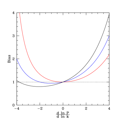
Appendix B Normalization bias for a power law spectrum

For a pure power law spectrum $P(k)\propto k^{-\alpha}$ the expression 26 can be easily evaluated and exact relation between $\tilde{P}(k_{r})$ and $P(k_{r})$ can be written. The shape of the spectrum is of course recovered correctly, while the normalization may differ slightly, caused by moving $P(k)$ outside the integral in eq. 27:

$$\frac{\tilde{P}}{P}=2^{\alpha/2}\frac{\Gamma(\frac{n}{2}+2-\frac{\alpha}{2})}{\Gamma(\frac{n}{2}+2)}.$$ (32)

Corresponding bias $\frac{\tilde{P}}{P}$ is shown in Fig. 21. One can see that for the most relevant problems (2D or 3D geometry, $\frac{d\ln P}{d\ln k}$ in the range [-3:0]) the bias is modest.

Figure 21: Bias $\frac{\tilde{P}}{P}$ in the normalization of the recovered spectrum for a pure power law power spectrum, as a function of slope for different dimensions of the problem (red - 1D, blue - 2D, black - 3D)

.

References

- Alfred & Hanssen (1997) Alfred & Hanssen 1997, Signal Processing, 58, 327
- Bensch et al. (2001) Bensch F., Stutzki J., Ossenkopf V., 2001, A&A, 366, 636
- Churazov et al. (2012) Churazov E., et al., 2012, MNRAS, 421, 1123
- Dolag et al. (2006) Dolag K., Meneghetti M., Moscardini L., Rasia E., Bonaldi A., 2006, MNRAS, 370, 656
- Emmanoulopoulos et al. (2010) Emmanoulopoulos D., McHardy I. M., Uttley P., 2010, MNRAS, 404, 931
- Fodor & Stark (2000) Fodor I., Stark P., 2000, Signal Processing, IEEE Transactions on, 48, 3472
- Fodor & Stark (1998) Fodor I. K., Stark P. B., 1998, in S. Korzennik ed., Structure and Dynamics of the Interior of the Sun and Sun-like Stars Vol. 418 of ESA Special Publication, Multitaper Spectrum Estimates. p. 171
- Kastendieck et al. (2011) Kastendieck M. A., Ashley M. C. B., Horns D., 2011, A&A, 531, A123
- Markowitz (2010) Markowitz A., 2010, ApJ, 724, 26
- Markowitz et al. (2003) Markowitz A., Edelson R., Vaughan S., Uttley P., George I. M., Griffiths R. E., Kaspi S., Lawrence A., McHardy I., Nandra K., Pounds K., Reeves J., Schurch N., Warwick R., 2003, ApJ, 593, 96
- McHardy et al. (2006) McHardy I. M., Koerding E., Knigge C., Uttley P., Fender R. P., 2006, Nature, 444, 730
- Ossenkopf et al. (2008) Ossenkopf V., Krips M., Stutzki J., 2008, A&A, 485, 917
- Papadakis et al. (2009) Papadakis I. E., Sobolewska M., Arevalo P., Markowitz A., McHardy I. M., Miller L., Reeves J. N., Turner T. J., 2009, A&A, 494, 905
- Scott et al. (2003) Scott D. M., Finger M. H., Wilson C. A., 2003, MNRAS, 344, 412
- Stutzki et al. (1998) Stutzki J., Bensch F., Heithausen A., Ossenkopf V., Zielinsky M., 1998, A&A, 336, 697
- Thomson (1982) Thomson D. J., 1982, IEEE Proceedings, 70, 1055
- Timmer & König (1995) Timmer J., König M., 1995, A&A, 300, 707
- Uttley et al. (2002) Uttley P., McHardy I. M., Papadakis I. E., 2002, MNRAS, 332, 231
- Wieczorek & Simons (2007) Wieczorek M. A., Simons F. J., 2007, Journal of Fourier Analysis and Applications, 13, 665