A graphical presentation of signal delays in the datasets of Weihs et al.

Abstract

A graphical presentation of the timing of avalanche photodiode events in the datasets from the experiment of Weihs et al. [Phys. Rev. Lett. 81, 5039 (1998)] makes manifest the existence of two types of signal delay: (1) The introduction of rapid switching of the input to a pair of transverse electro-optical modulators causes a delay of approximately 20 nanoseconds for a proportion of coincident avalanche photodiode events; this effect has been previously noted, but a different cause is suggested by the data as considered here. (2) There are delays that depend on in which avalanche photodiode an event occurs; this effect has also been previously noted even though it is only strongly apparent when the relative time difference between avalanche photodiode events is near the stated $0.5$ nanosecond accuracy of the timestamps (but it is identifiable because of 75 picosecond resolution). The cause of the second effect is a difference between signal delays for the four avalanche photodiodes, for which correction can be made by straightforward local adjustments (with almost no effect on the degree of violation of Bell-CHSH inequalities).

I introduction

There have been several analyses of the datasets generated by the experiment of Wiehs et al. WeihsExpt ; WeihsThesis . Two, due to Hnilo, Kovalsky, and Santiago HKS , and Adenier and Khrennikov AKJPhysB2006 , are particularly singled out by Weihs WeihsComment . More recently, Zhao et al. have analyzed the data as part of a program to construct a computational model that violates Bell inequalities Zhao .

The Weihs et al. datasets contain, for a number of runs, a recorded timestamp when an event occurred in any of four avalanche photodiodes (APDs), together with a binary record of the input to a transverse electro-optical modulator at the time of each APD event. The timestamps have an accuracy of 0.5 nanoseconds and a resolution of 75 picoseconds. The dataset for each run is in two locally recorded parts, labelled “Alice” and “Bob”, containing data collected at each end of the experiment. The published papers and these datasets are the principal historical record of the Weihs et al. experiment, which together satisfy Bohr’s requirement that an experiment must be classically described. At this level of description, the datasets are essentially a nonlocal, contextual classical description of the whole experiment’s results, which are well-known to be incompatible with a local, noncontextual classical particle model.

Section II describes a graphical presentation of three datasets, longdist35, locbell2, and bellstat1, which differs from previous analysis by using the difference between APD timings as a coordinate instead of considering coincidence of APD events as a binary value that is true if the difference between their timings is less than the width of a chosen window (which in the case of Weihs et al.’s analysis was 4 nanoseconds, which the data suggests as an appropriate width). The first of the three datasets considered uses two 500 meter fiber optic cables to distribute light from the central light source and a Parametric Down-Conversion (PDC) crystal to two remote sites, at each of which there is a transverse electro-optical modulator, the output of which is directed to a dynamically modified polarizer and thence to a pair of APDs; for the second and third of these datasets the transverse electro-optical modulators, the polarizers, and the two pairs of APDs are close to the light source and the PDC crystal. For the first two of these datasets, the input signals to the transverse electro-optical modulators are switched rapidly between two values, whereas for the third dataset there is a constant input signal to the transverse electro-optical modulators.

Figure 1: (Color online) 10 second by $\pm 200$ nanosecond window on approximately coincident events from Alice’s perspective for longdist35, with a single timing adjustment (described in Section II).

Figure 2: (Color online) 10 second by $\pm 3$ nanosecond window on approximately coincident events from Alice’s perspective for longdist35, with a single timing adjustment (described in Section II).

Figure 3: (Color online) 2 second by $\pm 50$ nanosecond window on approximately coincident events from Alice’s perspective for bellstat1, with a single timing adjustment (described in Section II).

The comparison of the first two datasets with the third dataset enables us to show in Section III that rapid switching of the inputs to the transverse electro-optical modulators causes a delay of approximately 20 nanoseconds for a proportion of coincident APD events. We also show in Section IV that there is a correlation of APD events with the relative timing of APD events, on a time-scale of approximately 1 nanosecond. It is clear that these correlations are caused by different timing delays for the two APD signal channels (as suggested to the author by Gregor Weihs), because adjusting the timings of the data for the two channels by a constant offset eliminates the effect. Both delays have been previously identified AgueroEtAl , however graphical presentation makes the delays more immediately apparent.

Larsson and Gill LG show that there is a “coincidence loophole” that is distinct from the “detection loophole”, which the Weihs et al. experiment is well-known not to close. The 1 nanosecond time-scale of the correlations described here, however, does not immediately suggest a communication protocol that would allow a hidden variable model to be constructed. In particular, the 1 nanosecond time-scale is less than the 4 nanosecond time-scale of typical window widths, so these correlations are in a different regime than the timing correlations that are hypothetically introduced by Zhao et al. Zhao as part of a hidden variable model.

Although essentially self-contained, the analysis of the Weihs et al. datasets that is described here is partly motivated by a random field perspective on quantum fields MorganBellRandomFields ; MorganRQKG ; MorganLieFields , which suggests a close look at the datasets using methods of (stochastic) signal analysis. In particular, precise differences of the relative timing of the coincidence of APD events seem more likely to be of interest from a field perspective, instead of the less detailed binary fact of approximate coincidence that is suggested by a quantized photon perspective. Methods of signal analysis are also adopted by Hnilo, Kovalsky, and Santiago HKS .

II A graphical presentation of the datasets

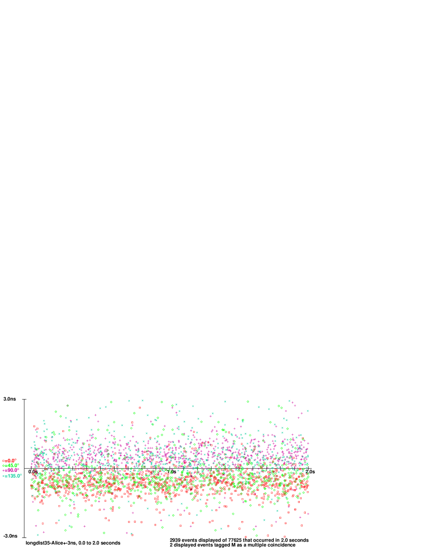
A C++ program was written to construct Embedded PostScript graphs for a given dataset, either from Alice’s perspective or from Bob’s perspective. For the case of Alice’s perspective, we plot the time difference $t_{A}-(t_{B}(t_{A})-\mathsf{offset})$ at each time $t_{A}$ at which there is an APD event at $A$ (Alice’s location), where $t_{B}(t_{A})-\mathsf{offset}$ is the closest time to $t_{A}$ at which there is an APD event at $B$ (Bob’s location), with an offset that allows for a slight difference between timestamps at $A$ and at $B$ that is more-or-less constant over time periods of ten seconds (the offsets for the datasets considered here, longdist35, locbell2, and bellstat1, are $+4$ nanoseconds, $-12.5$ nanoseconds, and $+10.7$ nanoseconds, respectively, with the sign reversed when considering Bob’s perspective). A negative value of $t_{A}-(t_{B}(t_{A})-\mathsf{offset})$ corresponds to an APD event at $A$ being earlier than the APD event at $B$ that is closest in time to it. At each coordinate $(t_{A},t_{A}-(t_{B}(t_{A})-\mathsf{offset}))$ a symbol is plotted that represents the binary input to the transverse electro-optical modulator, which for the datasets discussed correspond either to angles of $0^{\circ}$ or $45^{\circ}$ for Alice, or to angles of $22.5^{\circ}$ or $67.5^{\circ}$ for Bob. The symbol plotted also represents in which of the two APDs there was an event, which is taken to add $90^{\circ}$ to the angle. Internally, the numbers $0$, $1$, $2$, and $3$ are recorded, which correspond, for the datasets discussed, to angles $0^{\circ}$, $45^{\circ}$, $90^{\circ}$, and $135^{\circ}$ for Alice, and to angles $22.5^{\circ}$, $67.5^{\circ}$, $112.5^{\circ}$, and $147.5^{\circ}$ for Bob, which are represented graphically by a square, a diamond, a cross, and an “$\mathsf{x}$”. If the APD event at $A$ that is one of a coincident pair is close to more than one APD event at $B$, or if the APD event at $B$ that is one of a coincident pair is close to more than one APD event at $A$, the coincident pair is tagged as a multiple coincidence, represented graphically by an “M”, and ignored for the purposes of computing the violation of Bell-CHSH inequalities.

Figure 4: (Color online) 2 second by $\pm 3$ nanosecond window on approximately coincident events from Alice’s perspective for longdist35, with a single timing adjustment (described in Section II). There is a visible asymmetry between which events are observed relatively early at $A$ and which events are observed relatively late at $A$, compared to coincident events at $B$.

Figure 5: (Color online) 2 second by $\pm 3$ nanosecond window on approximately coincident events from Bob’s perspective for longdist35, with a single timing adjustment (described in Section II). The temporal asymmetry of events is less apparent than in Figure 4, but is still visible.

Figure 6: (Color online) 2 second by $\pm 3$ nanosecond window on approximately coincident events from Alice’s perspective for locbell2, with a single timing adjustment (described in Section II). The density of closely coincident events is greater because the transverse electro-optical modulator and APDs are not separated from the light source by 500 meters of fiber optic cable. The temporal asymmetry of events visible in Figures 4 and 5 is not visible here, but it can be made apparent using a graphical presentation such as Figure 9.

III Delays caused by the transverse electro-optical modulator

Figures 1 and 2 show a vertical $\pm 200$ nanosecond section and a vertical $\pm 3$ nanosecond section of the graph for the whole ten seconds of data for longdist35 from Alice’s perspective; subsequently we will show graphs for only the first two seconds of data, which are adequate for our purpose here, more readable, and result in smaller Embedded PostScript files. It is necessary to show different vertical sections of the graph to make different features of the data visually apparent. Note that there is a wide stripe within approximately $\pm 20$ nanoseconds in which there is a greater density of APD events, and a narrower stripe within approximately $\pm 1$ nanosecond in which there is a much greater density of APD events. The density of APD events beyond $\pm 20$ nanoseconds is approximately uniform. For comparison, the characteristic lengths of the elementary geometry of the experiment are a straight line separation between $A$ and $B$ of 400 meters and a separation between $A$ and $B$ along the fiber optic cable light guide of 1000 meters, corresponding to characteristic times of approximately 1.3 microseconds and 3.3 microseconds at the speed of light. In the vertical $\pm 3$ nanosecond section, an apparent drift of the relative times of APD events at $A$ and $B$ over 10 seconds is visible, which is consistent with properties of the clocks that are used to provide timestamps, described by Gregor Weihs as providing “a relative accuracy of $8\cdot 10^{-11}$, corresponding to $4.8$ [nanoseconds], for a $60$ [second] interval”WeihsComment . The more-or-less linear drift over a ten-second timescale allows for a straighforward adjustment of the timestamps.

The stripe of APD event pairs that are within $\pm 20$ nanoseconds of each other is also present in the dataset locbell2 (not shown), from both Alice’s and Bob’s perspective, but it is not present in the dataset bellstat1, for which a vertical $\pm 50$ nanosecond section is shown in Figure 3, nor in any of the datasets bellstat0, bellstat2, and bellstat3. The dataset bellstat1 is less than 2 seconds long; only two types of APD events are present because there is no switching of the transverse electro-optical modulator. Except for the dataset bellstat1, the binary input to the transverse electro-optical modulator is chosen randomly approximately every 100 nanoseconds. It takes approximately 14 nanoseconds to switch from one setting to another, during which time APD events are ignored WeihsComment . Given the different distribution of APD event pairs when there is no rapid switching of the transverse electro-optical modulator, and given that the 14 nanosecond period during which APD events are ignored is a comparable time-scale to the 20 nanosecond broadening of coincidences of APD events, it seems likely that the effect is caused by either electrical or optical properties of the rapid switching of the transverse electro-optical modulator. Agüero et al. suggest that the “cause is a drift between the clocks at stations $A$ and $B$” because their experiment uses a single clock and does not show a broadening of coincidences AgueroEtAl , however there is no reason to think that the clock is inaccurate on the relatively coarse scale of $\pm 20$ nanoseconds in the Weihs et al. experiment.

IV Timing correlations in long distance datasets

Figure 7: (Color online) 2 second by $\pm 3$ nanosecond window on approximately coincident events from Alice’s perspective for longdist35, adjusted for relative timing drift and for local detector delays.

Figure 8: (Color online) 2 second by $\pm 3$ nanosecond window on approximately coincident events from Bob’s perspective for longdist35, adjusted for relative timing drift and for local detector delays.

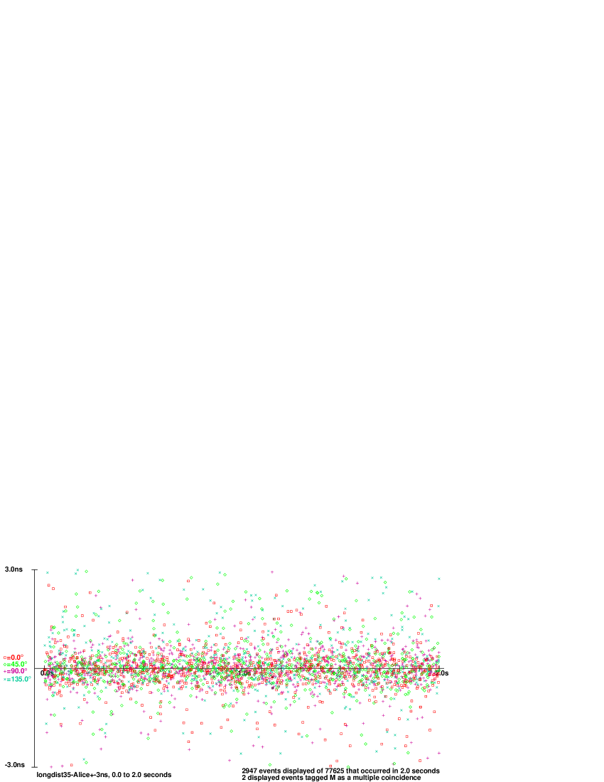
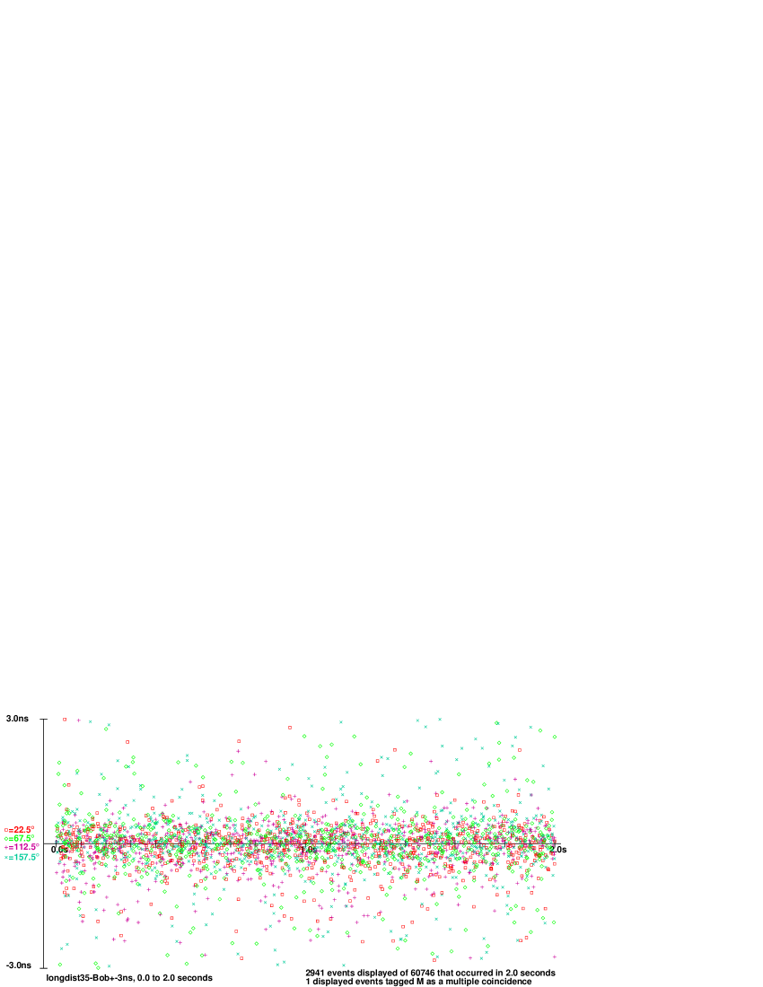
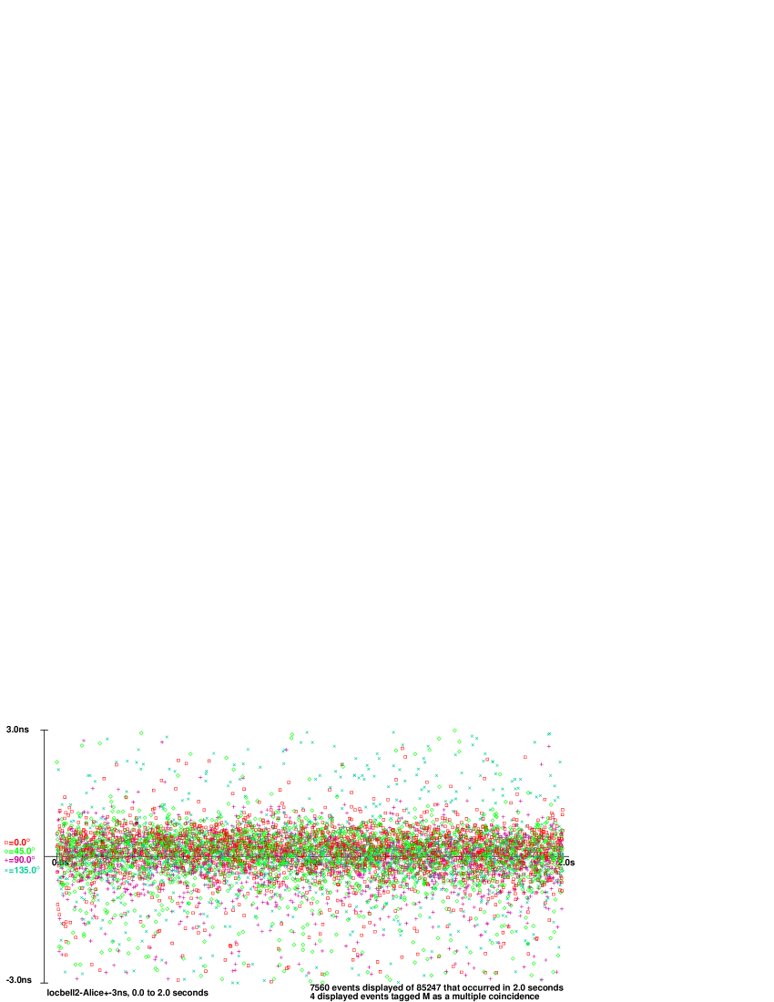
It is already apparent in Figure 2 that there is a strong correlation on a nanosecond scale between the direction associated with APD events at $A$ and the time difference between the APD events at $A$ and $B$. The correlation is easily visible in Figure 4, for the dataset longdist35 (and is equally visible for the dataset longdist34, which is not shown), but is not as evidently present in Figure 6, for the dataset locbell2, the difference being the extensive modification of the experimental apparatus necessary to introduce a much greater distance between the APDs and two lengths of 500 meters of fiber optic cable for longdist35 (and for longdist34).

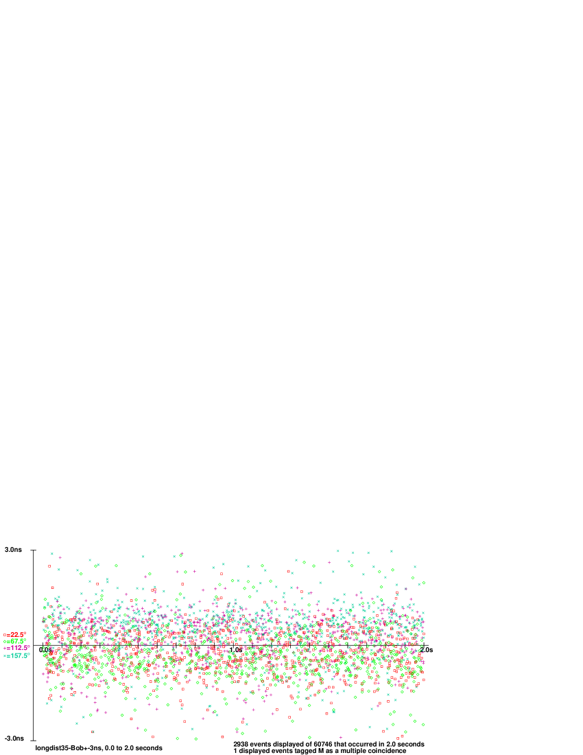
The precision of the correlation is greater from Alice’s perspective than from Bob’s perspective, as can be seen by comparison of Figures 4 and 5 (note that relative time difference from Bob’s perspective has the opposite sign to relative time difference from Alice’s perspective).

The apparent correlation can be eliminated, however, by essentially local adjustments that depend only on which APD the event occurred in, effectively because the electronics associated with the four APDs introduce slightly different delays. The consequent Figures 7 and 8 show the result of including both an adjustment for timing drift of 50ps per second and local detector adjustments of 0.0ns and 0.9ns for Alice and 4.4ns and 4.7ns for Bob, instead of a uniform less detailed adjustment of 4 nanoseconds between Alice and Bob that is used for Figures 4 and 5. The adjustments required for locbell2 are not as great.

V Conclusion

Although the rapid switching of the transverse electro-optical modulator does not change the signal enough to invalidate the results or interpretation of the Weihs et al. experiment, nonetheless it is a matter of concern that rapid switching introduces a distortion of APD event timings on a time-scale of 20 nanoseconds, which is enough to have a technological impact in some circumstances. The local adjustments for different signal delays for different detectors are relatively small and of marginal interest in the Weihs experiment.

VI Discussion

This paper is not intended for publication, so I include here fragmentary comments on quantum mechanical experiments —for which Bell-violating experiments have now become the most common example, replacing the old favorite, the double-slit experiment— that are rather disconnected from the analysis of Gregor Weihs’ experiment that is the paper’s main purpose, but that may be of interest to readers of the Bell inequality literature.

Although we can often describe experimental apparatus coarsely using operators and states that act on low-dimensional Hilbert spaces, it is a nontrivial task to construct experimental apparatus that can be described accurately in such simple terms. If we wish to describe an experimental apparatus accurately we generally must resort to quantum field models, unless we have taken great care to ensure that an experimental apparatus is dynamically elementary. This is analogous to descriptions of a pendulum as a simple harmonic oscillator, which may be quite accurate as a first approximation, even for something as complex as a child’s swing, but it is no small thing to construct a classical system that can be very accurately modeled as a simple harmonic oscillator, so that, for example, it may be used as an accurate clock. For the purposes of quantum computation and other technological applications of the mathematics of quantum theory, it is desirable to construct devices that are accurately describable using operators and states that act on low-dimensional Hilbert spaces, but it is a difficult engineering feat.

From a classical thermodynamics point of view, we expect the statistics of the APD events to be determined by the geometrical configuration of the whole apparatus, because the configuration of the experimental apparatus determines the properties of the coarse-grained equilibrium state of the electromagnetic field and of the PDC crystal and APDs that interact with it. Even though at a fine-grained level there are many non-equilibrium APD events, nonetheless in terms of those statistics of the properties of the APD events that are generally reproducible on time-scales of seconds or minutes, the experiment is at equilibrium. Indeed, it is precisely required that at least some statistics must be reproducible in order for us to claim that we are doing a Scientific experiment, but there is no rule about what statistics must be reproducible. A classical thermodynamic point of view is therefore in line with Bohr’s view that the configuration of the whole experimental apparatus conditions the experimental results. Furthermore, we observe discrete events only because we choose to design and use a thermodynamically metastable system such as an APD that is capable of making transitions between thermodynamically distinguishable states in different ways depending on its surrounding environment. We choose to condition the output signal from an APD to be a binary value, and to record the times at which the output signal makes a transition to its excited state, but at a more detailed level the output signal can be modeled as a continuous current, which is ultimately more appropriate if we adopt a field theoretic perspective to enable more detailed modeling of the APD as an integral part of the whole experimental apparatus. Thermodynamic transitions of an APD should, if ideally constructed, occur randomly, at a minimal dark rate, if there is no external signal, and statistics of dark rate APD events should exhibit as little statistically significant structure as possible, so that when we introduce an external signal, statistics of the APD events can be used to characterize the external signal as cleanly as possible.

Appendix A An alternative visualization

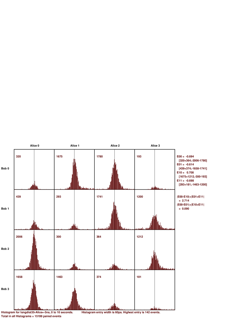
Figure 9 presents a visualization of the detector and instrument setting timing statistics, for a 3ns window in 60ps sections, for longdist35 from Alice’s perspective, adjusted for relative timing drift and for local detector delays, together with the corresponding calculation of the Bell-CHSH inequality violation, for the complete 10 second run. The vast majority of the detector coincidences are seen to lie within a $\pm$1ns window. The derivation of the necessary local detector adjustments for the limited number of datasets considered was done by eye, ensuring that as far as possible all 16 distributions are centered in this graphical presentation.

Figure 9: Visualization of the detector and instrument setting timing statistics, for a 3ns window in 60ps sections, for longdist35 from Alice’s perspective, adjusted for relative timing drift and for local detector delays, together with the corresponding calculation of the Bell-CHSH inequality violation. For Alice, $0$, $1$, $2$, and $3$ correspond to angles $0^{\circ}$, $45^{\circ}$, $90^{\circ}$, and $135^{\circ}$. For Bob, $0$, $1$, $2$, and $3$ correspond to angles $22.5^{\circ}$, $67.5^{\circ}$, $112.5^{\circ}$, and $147.5^{\circ}$.