Sensorless position estimation of Permanent-Magnet Synchronous Motors using a saturation model

Al Kassem Jebai, François Malrait, Philippe Martin and Pierre Rouchon A-K. Jebai, P. Martin and P. Rouchon are with the Centre Automatique et Systèmes, MINES ParisTech, 75006 Paris, France {al-kassem.jebai, philippe.martin, pierre.rouchon}@mines-paristech.frF. Malrait is with Schneider Toshiba Inverter Europe, 27120 Pacy-sur-Eure, France francois.malrait@schneider-electric.com
Abstract

Sensorless control of Permanent-Magnet Synchronous Motors (PMSM) at low velocity remains a challenging task. A now well-established method consists in injecting a high-frequency signal and use the rotor saliency, both geometric and magnetic-saturation induced. This paper proposes a clear and original analysis based on second-order averaging of how to recover the position information from signal injection; this analysis blends well with a general model of magnetic saturation. It also proposes a simple parametric model of the saturated PMSM, based on an energy function which simply encompasses saturation and cross-saturation effects. Experimental results on a surface-mounted PMSM and an interior magnet PMSM illustrate the relevance of the approach.

Index Terms:
Permanent-magnet synchronous motor, sensorless position estimation, signal injection, magnetic saturation, energy-based modeling, averaging.

I Introduction

Permanent-Magnet Synchronous Motors (PMSM) are widely used in industry. In the so-called “sensorless” mode of operation, the rotor position and velocity are not measured and the control law must make do with only current measurements. While sensorless control at medium to high velocities is well understood, with many reported control schemes and industrial products, sensorless control at low velocity remains a challenging task. The reason is that observability degenerates at zero velocity, causing a serious problem in the necessary rotor position estimation.

A now well-established method to overcome this problem is to add some persistent excitation by injecting a high-frequency signal [1] and use the rotor saliency, whether geometric for Interior Permanent-Magnet machines or induced by main flux saturation for Surface Permanent-Magnet machines [2, 3, 4, 5, 6, 7, 8, 9, 10]. Signal injection is moreover considered as a standard building block in hybrid control schemes for complete drives operating from zero to full speed [11, 12, 13, 14, 15].

However to get a good position estimation under high-load condition it is important to take cross-saturation into account [16, 17, 18, 19, 20, 21, 22, 23, 24, 25, 26]. It is thus necessary to rely on a model of the saturated PMSM adapted to control purposes, i.e. rich enough to capture in particular cross-saturation but also simple enough to be used in real-time and to be easily identified in the field; see [27, 28, 29, 30, 31, 32] for references more or less in this spirit.

The contribution of this paper, which builds on the preliminary work [33], is twofold: on the one hand it proposes a clear and original analysis based on second-order averaging of how to recover the position information from signal injection; this analysis can accommodate to any form of injected signals, e.g. square signals as in [34], and blends well with a general model of magnetic saturation including cross-saturation. On the other hand a simple parametric model of the saturated PMSM, well-adapted to control purposes, is introduced; it is based on an energy function which simply encompasses saturation and cross-saturation effects.

The paper runs as follows: section II presents the saturation model. In section III position estimation by signal injection is studied thanks to second-order averaging. Section IV is devoted to the estimation of the parameters entering the saturation model using once again signal injection and averaging. Finally section IV-C experimentally demonstrates on two kinds of motors (with interior magnets and surface-mounted magnets) the relevance of the approach and the necessity of considering saturation to correctly estimate the position.

II An energy-based model of the saturated PMSM

II-A Notations

In the sequel we denote by xij:=(xi,xj)Tassignsubscript𝑥𝑖𝑗superscriptsubscript𝑥𝑖subscript𝑥𝑗𝑇x_{ij}:=(x_{i},x_{j})^{T} the vector made from the real numbers xisubscript𝑥𝑖x_{i} and xjsubscript𝑥𝑗x_{j}, where ij𝑖𝑗ij can be dq𝑑𝑞dq, αβ𝛼𝛽\alpha\beta or γδ𝛾𝛿\gamma\delta. We also define the matrices

Mμ:=(cosμsinμsinμcosμ)and𝒦:=(0110),formulae-sequenceassignsubscript𝑀𝜇matrix𝜇𝜇𝜇𝜇andassign𝒦matrix0110M_{\mu}:=\begin{pmatrix}\cos\mu&-\sin\mu\\ \sin\mu&\cos\mu\end{pmatrix}\quad\text{and}\quad{\mathcal{K}}:=\begin{pmatrix}0&-1\\ 1&0\end{pmatrix},

and we have the useful relation

dMμdμ=𝒦Mμ=Mμ𝒦.𝑑subscript𝑀𝜇𝑑𝜇𝒦subscript𝑀𝜇subscript𝑀𝜇𝒦\frac{dM_{\mu}}{d\mu}={\mathcal{K}}M_{\mu}=M_{\mu}{\mathcal{K}}.

II-B Energy-based model

The model of a two-axis PMSM expressed in the synchronous dq𝑑𝑞d-q frame reads

dϕdqdt𝑑subscriptitalic-ϕ𝑑𝑞𝑑𝑡\displaystyle\frac{d\phi_{dq}}{dt} =udqRidqω𝒦(ϕdq+ϕm)absentsubscript𝑢𝑑𝑞𝑅subscript𝑖𝑑𝑞𝜔𝒦subscriptitalic-ϕ𝑑𝑞subscriptitalic-ϕ𝑚\displaystyle=u_{dq}-Ri_{dq}-{\omega}{\mathcal{K}}(\phi_{dq}+\phi_{m}) (1)
Jn2dωdt𝐽superscript𝑛2𝑑𝜔𝑑𝑡\displaystyle\frac{J}{n^{2}}\frac{d\omega}{dt} =32idqT𝒦(ϕdq+ϕm)τLnabsent32superscriptsubscript𝑖𝑑𝑞𝑇𝒦subscriptitalic-ϕ𝑑𝑞subscriptitalic-ϕ𝑚subscript𝜏𝐿𝑛\displaystyle=\frac{3}{2}i_{dq}^{T}{\mathcal{K}}(\phi_{dq}+\phi_{m})-\frac{\tau_{L}}{n} (2)
dθdt𝑑𝜃𝑑𝑡\displaystyle\frac{d\theta}{dt} =ω,absent𝜔\displaystyle=\omega, (3)

with ϕdqsubscriptitalic-ϕ𝑑𝑞\phi_{dq} flux linkage due to the current; ϕm:=(λ,0)Tassignsubscriptitalic-ϕ𝑚superscript𝜆0𝑇\phi_{m}:=(\lambda,0)^{T} constant flux linkage due to the permanent magnet; udqsubscript𝑢𝑑𝑞u_{dq} impressed voltage and idqsubscript𝑖𝑑𝑞i_{dq} stator current; ω𝜔\omega and θ𝜃\theta rotor (electrical) speed and position; R𝑅R stator resistance; n𝑛n number of pole pairs; J𝐽J inertia moment and τLsubscript𝜏𝐿\tau_{L} load torque. The physically impressed voltages are uαβ:=Mθudqassignsubscript𝑢𝛼𝛽subscript𝑀𝜃subscript𝑢𝑑𝑞u_{\alpha\beta}:=M_{\theta}u_{dq} while the physically measurable currents are iαβ:=Mθidqassignsubscript𝑖𝛼𝛽subscript𝑀𝜃subscript𝑖𝑑𝑞i_{\alpha\beta}:=M_{\theta}i_{dq}. The current can be expressed in function of the flux linkage thanks to a suitable energy function (ϕd,ϕq)subscriptitalic-ϕ𝑑subscriptitalic-ϕ𝑞{\mathcal{H}}(\phi_{d},\phi_{q}) by

idq=dq(ϕdq):=(1(ϕd,ϕq)2(ϕd,ϕq)),subscript𝑖𝑑𝑞subscript𝑑𝑞subscriptitalic-ϕ𝑑𝑞assignmatrixsubscript1subscriptitalic-ϕ𝑑subscriptitalic-ϕ𝑞subscript2subscriptitalic-ϕ𝑑subscriptitalic-ϕ𝑞\displaystyle i_{dq}={\mathcal{I}}_{dq}(\phi_{dq}):=\begin{pmatrix}\partial_{1}{\mathcal{H}}(\phi_{d},\phi_{q})\\ \partial_{2}{\mathcal{H}}(\phi_{d},\phi_{q})\end{pmatrix}, (4)

where ksubscript𝑘\partial_{k}{\mathcal{H}} denotes the partial derivative w.r.t. the kthsuperscript𝑘𝑡k^{th} variable [35, 36]; without loss of generality (0,0)=0000{\mathcal{H}}(0,0)=0. Such a relation between flux linkage and current naturally encompasses cross-saturation effects.

For an unsaturated PMSM this energy function reads

l(ϕd,ϕq)subscript𝑙subscriptitalic-ϕ𝑑subscriptitalic-ϕ𝑞\displaystyle{\mathcal{H}}_{l}(\phi_{d},\phi_{q}) =12Ldϕd2+12Lqϕq2absent12subscript𝐿𝑑subscriptsuperscriptitalic-ϕ2𝑑12subscript𝐿𝑞subscriptsuperscriptitalic-ϕ2𝑞\displaystyle=\frac{1}{2L_{d}}\phi^{2}_{d}+\frac{1}{2L_{q}}\phi^{2}_{q}

where Ldsubscript𝐿𝑑L_{d} and Lqsubscript𝐿𝑞L_{q} are the motor self-inductances, and we recover the usual linear relations

idsubscript𝑖𝑑\displaystyle i_{d} =1l(ϕd,ϕq)=ϕdLdabsentsubscript1subscript𝑙subscriptitalic-ϕ𝑑subscriptitalic-ϕ𝑞subscriptitalic-ϕ𝑑subscript𝐿𝑑\displaystyle=\partial_{1}{\mathcal{H}}_{l}(\phi_{d},\phi_{q})=\frac{\phi_{d}}{L_{d}}
iqsubscript𝑖𝑞\displaystyle i_{q} =2l(ϕd,ϕq)=ϕqLq.absentsubscript2subscript𝑙subscriptitalic-ϕ𝑑subscriptitalic-ϕ𝑞subscriptitalic-ϕ𝑞subscript𝐿𝑞\displaystyle=\partial_{2}{\mathcal{H}}_{l}(\phi_{d},\phi_{q})=\frac{\phi_{q}}{L_{q}}.

Notice the expression for {\mathcal{H}} should respect the symmetry of the PMSM w.r.t the direct axis, i.e.

(ϕd,ϕq)=(ϕd,ϕq),subscriptitalic-ϕ𝑑subscriptitalic-ϕ𝑞subscriptitalic-ϕ𝑑subscriptitalic-ϕ𝑞{\mathcal{H}}(\phi_{d},-\phi_{q})={\mathcal{H}}(\phi_{d},\phi_{q}), (5)

which is obviously the case for lsubscript𝑙{\mathcal{H}}_{l}. Indeed (1)–(3) is left unchanged by the transformation

(ud,uq,ϕd,ϕq,id,iq,ω,θ,τL)(ud,uq,ϕd,ϕq,id,iq,ω,θ,τL).subscript𝑢𝑑subscript𝑢𝑞subscriptitalic-ϕ𝑑subscriptitalic-ϕ𝑞subscript𝑖𝑑subscript𝑖𝑞𝜔𝜃subscript𝜏𝐿subscript𝑢𝑑subscript𝑢𝑞subscriptitalic-ϕ𝑑subscriptitalic-ϕ𝑞subscript𝑖𝑑subscript𝑖𝑞𝜔𝜃subscript𝜏𝐿(u_{d},u_{q},\phi_{d},\phi_{q},i_{d},i_{q},{\omega},\theta,\tau_{L})\rightarrow\\ (u_{d},-u_{q},\phi_{d},-\phi_{q},i_{d},-i_{q},-{\omega},-\theta,-\tau_{L}).

II-C Parametric description of magnetic saturation

Magnetic saturation can be accounted for by considering a more complicated magnetic energy function {\mathcal{H}}, having lsubscript𝑙{\mathcal{H}}_{l} for quadratic part but including also higher-order terms. From experiments saturation effects are well captured by considering only third- and fourth-order terms, hence

(ϕd,ϕq)=l(ϕd,ϕq)+i=03α3i,iϕd3iϕqi+i=04α4i,iϕd4iϕqi.subscriptitalic-ϕ𝑑subscriptitalic-ϕ𝑞subscript𝑙subscriptitalic-ϕ𝑑subscriptitalic-ϕ𝑞superscriptsubscript𝑖03subscript𝛼3𝑖𝑖superscriptsubscriptitalic-ϕ𝑑3𝑖superscriptsubscriptitalic-ϕ𝑞𝑖superscriptsubscript𝑖04subscript𝛼4𝑖𝑖superscriptsubscriptitalic-ϕ𝑑4𝑖superscriptsubscriptitalic-ϕ𝑞𝑖{\mathcal{H}}(\phi_{d},\phi_{q})={\mathcal{H}}_{l}(\phi_{d},\phi_{q})\\ +\sum_{i=0}^{3}\alpha_{3-i,i}\phi_{d}^{3-i}\phi_{q}^{i}+\sum_{i=0}^{4}\alpha_{4-i,i}\phi_{d}^{4-i}\phi_{q}^{i}.

This is a perturbative model where the higher-order terms appear as corrections of the dominant term lsubscript𝑙{\mathcal{H}}_{l}. The nine coefficients αijsubscript𝛼𝑖𝑗\alpha_{ij} together with Ldsubscript𝐿𝑑L_{d}, Lqsubscript𝐿𝑞L_{q} are motor dependent. But (5) implies α2,1=α0,3=α3,1=α1,3=0subscript𝛼21subscript𝛼03subscript𝛼31subscript𝛼130\alpha_{2,1}=\alpha_{0,3}=\alpha_{3,1}=\alpha_{1,3}=0, so that the energy function eventually reads

(ϕd,ϕq)=l(ϕd,ϕq)+α3,0ϕd3+α1,2ϕdϕq2+α4,0ϕd4+α2,2ϕd2ϕq2+α0,4ϕq4.subscriptitalic-ϕ𝑑subscriptitalic-ϕ𝑞subscript𝑙subscriptitalic-ϕ𝑑subscriptitalic-ϕ𝑞subscript𝛼30superscriptsubscriptitalic-ϕ𝑑3subscript𝛼12subscriptitalic-ϕ𝑑superscriptsubscriptitalic-ϕ𝑞2subscript𝛼40superscriptsubscriptitalic-ϕ𝑑4subscript𝛼22superscriptsubscriptitalic-ϕ𝑑2superscriptsubscriptitalic-ϕ𝑞2subscript𝛼04superscriptsubscriptitalic-ϕ𝑞4{\mathcal{H}}(\phi_{d},\phi_{q})={\mathcal{H}}_{l}(\phi_{d},\phi_{q})+\alpha_{3,0}\phi_{d}^{3}+\alpha_{1,2}\phi_{d}\phi_{q}^{2}\\ +\alpha_{4,0}\phi_{d}^{4}+\alpha_{2,2}\phi_{d}^{2}\phi_{q}^{2}+\alpha_{0,4}\phi_{q}^{4}. (6)

From (4) and (6) the currents are then explicitly given by

idsubscript𝑖𝑑\displaystyle i_{d} =ϕdLd+3α3,0ϕd2+α1,2ϕq2+4α4,0ϕd3+2α2,2ϕdϕq2absentsubscriptitalic-ϕ𝑑subscript𝐿𝑑3subscript𝛼30superscriptsubscriptitalic-ϕ𝑑2subscript𝛼12superscriptsubscriptitalic-ϕ𝑞24subscript𝛼40superscriptsubscriptitalic-ϕ𝑑32subscript𝛼22subscriptitalic-ϕ𝑑superscriptsubscriptitalic-ϕ𝑞2\displaystyle=\frac{\phi_{d}}{L_{d}}+3\alpha_{3,0}\phi_{d}^{2}+\alpha_{1,2}\phi_{q}^{2}+4\alpha_{4,0}\phi_{d}^{3}+2\alpha_{2,2}\phi_{d}\phi_{q}^{2} (7)
iqsubscript𝑖𝑞\displaystyle i_{q} =ϕqLq+2α1,2ϕdϕq+2α2,2ϕd2ϕq+4α0,4ϕq3,absentsubscriptitalic-ϕ𝑞subscript𝐿𝑞2subscript𝛼12subscriptitalic-ϕ𝑑subscriptitalic-ϕ𝑞2subscript𝛼22superscriptsubscriptitalic-ϕ𝑑2subscriptitalic-ϕ𝑞4subscript𝛼04superscriptsubscriptitalic-ϕ𝑞3\displaystyle=\frac{\phi_{q}}{L_{q}}+2\alpha_{1,2}\phi_{d}\phi_{q}+2\alpha_{2,2}\phi_{d}^{2}\phi_{q}+4\alpha_{0,4}\phi_{q}^{3}, (8)

which are the so-called flux-current magnetization curves.

To conclude, the model of the saturated PMSM is given by (1)–(3) and (7)-(8), with ϕd,ϕq,ω,θsubscriptitalic-ϕ𝑑subscriptitalic-ϕ𝑞𝜔𝜃\phi_{d},\phi_{q},{\omega},\theta as state variables. The magnetic saturation effects are represented by the five parameters α3,0,α1,2,α4,0,α2,2,α0,4subscript𝛼30subscript𝛼12subscript𝛼40subscript𝛼22subscript𝛼04\alpha_{3,0},\alpha_{1,2},\alpha_{4,0},\alpha_{2,2},\alpha_{0,4}.

II-D Model with id,iqsubscript𝑖𝑑subscript𝑖𝑞i_{d},i_{q} as state variables

The model of the PMSM is usually expressed with currents as state variables. This can be achieved here by time differentiating idq=dq(ϕdq)subscript𝑖𝑑𝑞subscript𝑑𝑞subscriptitalic-ϕ𝑑𝑞i_{dq}={\mathcal{I}}_{dq}(\phi_{dq}),

didqdt=Ddq(ϕdq)dϕdqdt,𝑑subscript𝑖𝑑𝑞𝑑𝑡𝐷subscript𝑑𝑞subscriptitalic-ϕ𝑑𝑞𝑑subscriptitalic-ϕ𝑑𝑞𝑑𝑡\displaystyle\frac{di_{dq}}{dt}=D{\mathcal{I}}_{dq}(\phi_{dq})\frac{d\phi_{dq}}{dt},

with dϕdqdt𝑑subscriptitalic-ϕ𝑑𝑞𝑑𝑡\frac{d\phi_{dq}}{dt} given by (1). Fluxes are then expressed as ϕdq=dq1(idq)subscriptitalic-ϕ𝑑𝑞superscriptsubscript𝑑𝑞1subscript𝑖𝑑𝑞\phi_{dq}={\mathcal{I}}_{dq}^{-1}(i_{dq}) by inverting the nonlinear relations (7)-(8); rather than performing the exact inversion, we can take advantage of the fact the coefficients αi,jsubscript𝛼𝑖𝑗\alpha_{i,j} are experimentally small. At first order w.r.t. the αi,jsubscript𝛼𝑖𝑗\alpha_{i,j} we have ϕd=Ldid+𝒪(|αi,j|)subscriptitalic-ϕ𝑑subscript𝐿𝑑subscript𝑖𝑑𝒪subscript𝛼𝑖𝑗\phi_{d}=L_{d}i_{d}+{\mathcal{O}}(\left\lvert\alpha_{i,j}\right\rvert) and ϕq=Lqiq+𝒪(|αi,j|)subscriptitalic-ϕ𝑞subscript𝐿𝑞subscript𝑖𝑞𝒪subscript𝛼𝑖𝑗\phi_{q}=L_{q}i_{q}+{\mathcal{O}}(\left\lvert\alpha_{i,j}\right\rvert); plugging these expressions into (7)-(8) and neglecting 𝒪(|αi,j|2)𝒪superscriptsubscript𝛼𝑖𝑗2{\mathcal{O}}(\left\lvert\alpha_{i,j}\right\rvert^{2}) terms, we easily find

ϕdsubscriptitalic-ϕ𝑑\displaystyle\phi_{d} =Ld(id3α3,0Ld2id2α1,2Lq2iq2\displaystyle=L_{d}\bigl{(}i_{d}-3\alpha_{3,0}L_{d}^{2}i_{d}^{2}-\alpha_{1,2}L_{q}^{2}i_{q}^{2}
4α4,0Ld3id32α2,2LdLq2idiq2)\displaystyle\quad\qquad-4\alpha_{4,0}L_{d}^{3}i_{d}^{3}-2\alpha_{2,2}L_{d}L_{q}^{2}i_{d}i_{q}^{2}\bigr{)} (9)
ϕqsubscriptitalic-ϕ𝑞\displaystyle\phi_{q} =Lq(iq2α1,2LdLqidiq\displaystyle=L_{q}\bigl{(}i_{q}-2\alpha_{1,2}L_{d}L_{q}i_{d}i_{q}-
2α2,2Ld2Lqid2iq4α0,4Lq3iq3).\displaystyle\quad\qquad 2\alpha_{2,2}L_{d}^{2}L_{q}i_{d}^{2}i_{q}-4\alpha_{0,4}L_{q}^{3}i_{q}^{3}\bigr{)}. (10)

Notice the matrix

(Gdd(idq)Gdq(idq)Gdq(idq)Gqq(idq)):=Ddq(dq1(idq)),assignmatrixsubscript𝐺𝑑𝑑subscript𝑖𝑑𝑞subscript𝐺𝑑𝑞subscript𝑖𝑑𝑞subscript𝐺𝑑𝑞subscript𝑖𝑑𝑞subscript𝐺𝑞𝑞subscript𝑖𝑑𝑞𝐷subscript𝑑𝑞superscriptsubscript𝑑𝑞1subscript𝑖𝑑𝑞\begin{pmatrix}G_{dd}(i_{dq})&G_{dq}(i_{dq})\\ G_{dq}(i_{dq})&G_{qq}(i_{dq})\end{pmatrix}:=D{\mathcal{I}}_{dq}\bigl{(}{\mathcal{I}}_{dq}^{-1}(i_{dq})\bigr{)}, (11)

with coefficients easily found to be

Gdd(idq)subscript𝐺𝑑𝑑subscript𝑖𝑑𝑞\displaystyle G_{dd}(i_{dq}) =1Ld+6α3,0Ldid+12α4,0Ld2id2+2α2,2Lq2iq2absent1subscript𝐿𝑑6subscript𝛼30subscript𝐿𝑑subscript𝑖𝑑12subscript𝛼40superscriptsubscript𝐿𝑑2superscriptsubscript𝑖𝑑22subscript𝛼22superscriptsubscript𝐿𝑞2superscriptsubscript𝑖𝑞2\displaystyle=\frac{1}{L_{d}}+6\alpha_{3,0}L_{d}i_{d}+12\alpha_{4,0}L_{d}^{2}i_{d}^{2}+2\alpha_{2,2}L_{q}^{2}i_{q}^{2}
Gdq(idq)subscript𝐺𝑑𝑞subscript𝑖𝑑𝑞\displaystyle G_{dq}(i_{dq}) =2α1,2Lqiq+4α2,2LdidLqiqabsent2subscript𝛼12subscript𝐿𝑞subscript𝑖𝑞4subscript𝛼22subscript𝐿𝑑subscript𝑖𝑑subscript𝐿𝑞subscript𝑖𝑞\displaystyle=2\alpha_{1,2}L_{q}i_{q}+4\alpha_{2,2}L_{d}i_{d}L_{q}i_{q}
Gqq(idq)subscript𝐺𝑞𝑞subscript𝑖𝑑𝑞\displaystyle G_{qq}(i_{dq}) =1Lq+2α1,2Ldid+2α2,2Ld2id2+12α0,4Lq2iq2,absent1subscript𝐿𝑞2subscript𝛼12subscript𝐿𝑑subscript𝑖𝑑2subscript𝛼22superscriptsubscript𝐿𝑑2superscriptsubscript𝑖𝑑212subscript𝛼04superscriptsubscript𝐿𝑞2superscriptsubscript𝑖𝑞2\displaystyle=\frac{1}{L_{q}}+2\alpha_{1,2}L_{d}i_{d}+2\alpha_{2,2}L_{d}^{2}i_{d}^{2}+12\alpha_{0,4}L_{q}^{2}i_{q}^{2},

is by construction symmetric; indeed

Ddq(ϕdq)=(11(ϕd,ϕq)21(ϕd,ϕq)12(ϕd,ϕq)22(ϕd,ϕq))𝐷subscript𝑑𝑞subscriptitalic-ϕ𝑑𝑞matrixsubscript11subscriptitalic-ϕ𝑑subscriptitalic-ϕ𝑞subscript21subscriptitalic-ϕ𝑑subscriptitalic-ϕ𝑞subscript12subscriptitalic-ϕ𝑑subscriptitalic-ϕ𝑞subscript22subscriptitalic-ϕ𝑑subscriptitalic-ϕ𝑞\displaystyle D\mathcal{I}_{dq}(\phi_{dq})=\begin{pmatrix}\partial_{11}{\mathcal{H}}(\phi_{d},\phi_{q})&\partial_{21}{\mathcal{H}}(\phi_{d},\phi_{q})\\ \partial_{12}{\mathcal{H}}(\phi_{d},\phi_{q})&\partial_{22}{\mathcal{H}}(\phi_{d},\phi_{q})\end{pmatrix}

and 12=21subscript12subscript21\partial_{12}{\mathcal{H}}=\partial_{21}{\mathcal{H}}. Therefore the inductance matrix

(Ldd(idq)Ldq(idq)Ldq(idq)Lqq(idq)):=assignmatrixsubscript𝐿𝑑𝑑subscript𝑖𝑑𝑞subscript𝐿𝑑𝑞subscript𝑖𝑑𝑞subscript𝐿𝑑𝑞subscript𝑖𝑑𝑞subscript𝐿𝑞𝑞subscript𝑖𝑑𝑞absent\displaystyle\begin{pmatrix}L_{dd}(i_{dq})&L_{dq}(i_{dq})\\ L_{dq}(i_{dq})&L_{qq}(i_{dq})\end{pmatrix}:= (Gdd(idq)Gdq(idq)Gdq(idq)Gqq(idq))1.superscriptmatrixsubscript𝐺𝑑𝑑subscript𝑖𝑑𝑞subscript𝐺𝑑𝑞subscript𝑖𝑑𝑞subscript𝐺𝑑𝑞subscript𝑖𝑑𝑞subscript𝐺𝑞𝑞subscript𝑖𝑑𝑞1\displaystyle\begin{pmatrix}G_{dd}(i_{dq})&G_{dq}(i_{dq})\\ G_{dq}(i_{dq})&G_{qq}(i_{dq})\end{pmatrix}^{-1}.

is also symmetric, though this is not always acknowledged in saturation models encountered in the literature.

III Position estimation by high frequency voltage injection

III-A Signal injection and averaging

A general sensorless control law can be expressed as

uαβsubscript𝑢𝛼𝛽\displaystyle u_{\alpha\beta} =Mθcuγδabsentsubscript𝑀subscript𝜃𝑐subscript𝑢𝛾𝛿\displaystyle=M_{\theta_{c}}u_{\gamma\delta} (12)
dθcdt𝑑subscript𝜃𝑐𝑑𝑡\displaystyle\frac{d\theta_{c}}{dt} =ωcabsentsubscript𝜔𝑐\displaystyle=\omega_{c} (13)
dηdt𝑑𝜂𝑑𝑡\displaystyle\frac{d\eta}{dt} =a(Mθciγδ,θc,η,t)absent𝑎subscript𝑀subscript𝜃𝑐subscript𝑖𝛾𝛿subscript𝜃𝑐𝜂𝑡\displaystyle=a\bigl{(}M_{\theta_{c}}i_{\gamma\delta},\theta_{c},\eta,t\bigr{)} (14)
ωcsubscript𝜔𝑐\displaystyle\omega_{c} =Ωc(Mθciγδ,θc,η,t)absentsubscriptΩ𝑐subscript𝑀subscript𝜃𝑐subscript𝑖𝛾𝛿subscript𝜃𝑐𝜂𝑡\displaystyle={\Omega}_{c}\bigl{(}M_{\theta_{c}}i_{\gamma\delta},\theta_{c},\eta,t\bigr{)} (15)
uγδsubscript𝑢𝛾𝛿\displaystyle u_{\gamma\delta} =𝒰γδ(Mθciγδ,θc,η,t),absentsubscript𝒰𝛾𝛿subscript𝑀subscript𝜃𝑐subscript𝑖𝛾𝛿subscript𝜃𝑐𝜂𝑡\displaystyle=\mathcal{U}_{\gamma\delta}\bigl{(}M_{\theta_{c}}i_{\gamma\delta},\theta_{c},\eta,t\bigr{)}, (16)

where the measured currents iαβ=Mθciγδsubscript𝑖𝛼𝛽subscript𝑀subscript𝜃𝑐subscript𝑖𝛾𝛿i_{\alpha\beta}=M_{\theta_{c}}i_{\gamma\delta} are used to compute uγδsubscript𝑢𝛾𝛿u_{\gamma\delta}, ωcsubscript𝜔𝑐\omega_{c} and the evolution of the internal (vector) variable η𝜂\eta of the controller; θcsubscript𝜃𝑐\theta_{c} and ωcsubscript𝜔𝑐\omega_{c} are known by design.

It will be convenient to write the system equations (1)–(3) in the γδ𝛾𝛿\gamma-\delta frame defined by xγδ:=Mθθcxdqassignsubscript𝑥𝛾𝛿subscript𝑀𝜃subscript𝜃𝑐subscript𝑥𝑑𝑞x_{\gamma\delta}:=M_{\theta-\theta_{c}}x_{dq}, which gives

dϕγδdt𝑑subscriptitalic-ϕ𝛾𝛿𝑑𝑡\displaystyle\frac{d\phi_{\gamma\delta}}{dt} =uγδRiγδωc𝒦ϕγδω𝒦Mθθcϕmabsentsubscript𝑢𝛾𝛿𝑅subscript𝑖𝛾𝛿subscript𝜔𝑐𝒦subscriptitalic-ϕ𝛾𝛿𝜔𝒦subscript𝑀𝜃subscript𝜃𝑐subscriptitalic-ϕ𝑚\displaystyle=u_{\gamma\delta}-Ri_{\gamma\delta}-{\omega}_{c}{\mathcal{K}}\phi_{\gamma\delta}-{\omega}{\mathcal{K}}M_{\theta-\theta_{c}}\phi_{m} (17)
Jn2dωdt𝐽superscript𝑛2𝑑𝜔𝑑𝑡\displaystyle\frac{J}{n^{2}}\frac{d\omega}{dt} =32iγδT𝒦(ϕγδ+Mθθcϕm)τLnabsent32superscriptsubscript𝑖𝛾𝛿𝑇𝒦subscriptitalic-ϕ𝛾𝛿subscript𝑀𝜃subscript𝜃𝑐subscriptitalic-ϕ𝑚subscript𝜏𝐿𝑛\displaystyle=\frac{3}{2}i_{\gamma\delta}^{T}{\mathcal{K}}(\phi_{\gamma\delta}+M_{\theta-\theta_{c}}\phi_{m})-\frac{\tau_{L}}{n} (18)
dθdt𝑑𝜃𝑑𝑡\displaystyle\frac{d\theta}{dt} =ω,absent𝜔\displaystyle=\omega, (19)

where from (7)-(8) currents and fluxes are related by

iγδ=Mθθcdq(MθθcTϕγδ).subscript𝑖𝛾𝛿subscript𝑀𝜃subscript𝜃𝑐subscript𝑑𝑞subscriptsuperscript𝑀𝑇𝜃subscript𝜃𝑐subscriptitalic-ϕ𝛾𝛿i_{\gamma\delta}=M_{\theta-\theta_{c}}\mathcal{I}_{dq}(M^{T}_{\theta-\theta_{c}}\phi_{\gamma\delta}). (20)

To estimate the position we will superimpose on some desirable control law (16) a fast-varying pulsating voltage,

uγδ=𝒰γδ(Mθciγδ,θc,η,t)+u~γδf(Ωt),subscript𝑢𝛾𝛿subscript𝒰𝛾𝛿subscript𝑀subscript𝜃𝑐subscript𝑖𝛾𝛿subscript𝜃𝑐𝜂𝑡subscript~𝑢𝛾𝛿𝑓Ω𝑡u_{\gamma\delta}=\mathcal{U}_{\gamma\delta}\bigl{(}M_{\theta_{c}}i_{\gamma\delta},\theta_{c},\eta,t\bigr{)}+\widetilde{u}_{\gamma\delta}f(\Omega t), (21)

where f𝑓f is a 2π2𝜋2\pi-periodic function with zero mean and u~γδsubscript~𝑢𝛾𝛿\widetilde{u}_{\gamma\delta} could like 𝒰γδsubscript𝒰𝛾𝛿\cal U_{\gamma\delta} depend on Mθciγδ,θc,η,tsubscript𝑀subscript𝜃𝑐subscript𝑖𝛾𝛿subscript𝜃𝑐𝜂𝑡M_{\theta_{c}}i_{\gamma\delta},\theta_{c},\eta,t (though it is always taken constant in the sequel). The constant pulsation ΩΩ\Omega is chosen “large”, so that f(Ωt)𝑓Ω𝑡f(\Omega t) can be seen as a “fast” oscillation; typically Ω:=2π×500rad/sassignΩ2𝜋500rad/s\Omega:=2\pi\times 500\,\text{rad/s} in the experiments in section IV-C.

If we apply this modified control law to (17)–(19), then it can be shown the solution of the closed loop system is

ϕγδsubscriptitalic-ϕ𝛾𝛿\displaystyle\phi_{\gamma\delta} =ϕ¯γδ+u~γδΩF(Ωt)+𝒪(1Ω2)absentsubscript¯italic-ϕ𝛾𝛿subscript~𝑢𝛾𝛿Ω𝐹Ω𝑡𝒪1superscriptΩ2\displaystyle=\overline{\phi}_{\gamma\delta}+\frac{\widetilde{u}_{\gamma\delta}}{\Omega}F(\Omega t)+{\mathcal{O}}{(\frac{1}{\Omega^{2}})} (22)
ω𝜔\displaystyle\omega =ω¯+𝒪(1Ω2)absent¯𝜔𝒪1superscriptΩ2\displaystyle=\overline{\omega}+{\mathcal{O}}{(\frac{1}{\Omega^{2}})} (23)
θ𝜃\displaystyle\theta =θ¯+𝒪(1Ω2)absent¯𝜃𝒪1superscriptΩ2\displaystyle=\overline{\theta}+{\mathcal{O}}{(\frac{1}{\Omega^{2}})} (24)
θcsubscript𝜃𝑐\displaystyle\theta_{c} =θ¯c+𝒪(1Ω2)absentsubscript¯𝜃𝑐𝒪1superscriptΩ2\displaystyle=\overline{\theta}_{c}+{\mathcal{O}}{(\frac{1}{\Omega^{2}})} (25)
η𝜂\displaystyle\eta =η¯+𝒪(1Ω2),absent¯𝜂𝒪1superscriptΩ2\displaystyle=\overline{\eta}+{\mathcal{O}}{(\frac{1}{\Omega^{2}})}, (26)

where F𝐹F is the primitive of f𝑓f with zero mean (F𝐹F clearly has the same period as f𝑓f); (ϕ¯γδ,ω¯,θ¯,θ¯c,η¯)subscript¯italic-ϕ𝛾𝛿¯𝜔¯𝜃subscript¯𝜃𝑐¯𝜂(\overline{\phi}_{\gamma\delta},\overline{\omega},\overline{\theta},\overline{\theta}_{c},\overline{\eta}) is the “slowly-varying” component of (ϕγδ,ω,θ,θc,η)subscriptitalic-ϕ𝛾𝛿𝜔𝜃subscript𝜃𝑐𝜂(\phi_{\gamma\delta},\omega,\theta,\theta_{c},\eta), i.e. satisfies

dϕ¯γδdt𝑑subscript¯italic-ϕ𝛾𝛿𝑑𝑡\displaystyle\frac{d\overline{\phi}_{\gamma\delta}}{dt} =u¯γδRi¯γδω¯c𝒦ϕ¯γδω𝒦Mθ¯θ¯cϕmabsentsubscript¯𝑢𝛾𝛿𝑅subscript¯𝑖𝛾𝛿subscript¯𝜔𝑐𝒦subscript¯italic-ϕ𝛾𝛿𝜔𝒦subscript𝑀¯𝜃subscript¯𝜃𝑐subscriptitalic-ϕ𝑚\displaystyle=\overline{u}_{\gamma\delta}-R\overline{i}_{\gamma\delta}-\overline{\omega}_{c}{\mathcal{K}}\overline{\phi}_{\gamma\delta}-{\omega}{\mathcal{K}}M_{\overline{\theta}-\overline{\theta}_{c}}\phi_{m}
Jn2dω¯dt𝐽superscript𝑛2𝑑¯𝜔𝑑𝑡\displaystyle\frac{J}{n^{2}}\frac{d\overline{\omega}}{dt} =32i¯γδT𝒦(ϕ¯γδ+Mθ¯θ¯cϕm)τLnabsent32superscriptsubscript¯𝑖𝛾𝛿𝑇𝒦subscript¯italic-ϕ𝛾𝛿subscript𝑀¯𝜃subscript¯𝜃𝑐subscriptitalic-ϕ𝑚subscript𝜏𝐿𝑛\displaystyle=\frac{3}{2}\overline{i}_{\gamma\delta}^{T}{\mathcal{K}}(\overline{\phi}_{\gamma\delta}+M_{\overline{\theta}-\overline{\theta}_{c}}\phi_{m})-\frac{\tau_{L}}{n}
dθ¯dt𝑑¯𝜃𝑑𝑡\displaystyle\frac{d\overline{\theta}}{dt} =ω¯absent¯𝜔\displaystyle=\overline{\omega}
dθ¯cdt𝑑subscript¯𝜃𝑐𝑑𝑡\displaystyle\frac{d\overline{\theta}_{c}}{dt} =ω¯cabsentsubscript¯𝜔𝑐\displaystyle=\overline{\omega}_{c}
dη¯dt𝑑¯𝜂𝑑𝑡\displaystyle\frac{d\overline{\eta}}{dt} =a(Mθ¯ci¯γδ,θ¯c,η¯,t),absent𝑎subscript𝑀subscript¯𝜃𝑐subscript¯𝑖𝛾𝛿subscript¯𝜃𝑐¯𝜂𝑡\displaystyle=a\bigl{(}M_{\overline{\theta}_{c}}\overline{i}_{\gamma\delta},\overline{\theta}_{c},\overline{\eta},t\bigr{)},

where

i¯γδsubscript¯𝑖𝛾𝛿\displaystyle\overline{i}_{\gamma\delta} =Mθ¯θ¯cdq(Mθ¯θ¯cTϕ¯γδ)absentsubscript𝑀¯𝜃subscript¯𝜃𝑐subscript𝑑𝑞subscriptsuperscript𝑀𝑇¯𝜃subscript¯𝜃𝑐subscript¯italic-ϕ𝛾𝛿\displaystyle=M_{\overline{\theta}-\overline{\theta}_{c}}\mathcal{I}_{dq}(M^{T}_{\overline{\theta}-\overline{\theta}_{c}}\overline{\phi}_{\gamma\delta}) (27)
ω¯csubscript¯𝜔𝑐\displaystyle\overline{\omega}_{c} =Ωc(Mθ¯ci¯γδ,θ¯c,η¯,t)absentsubscriptΩ𝑐subscript𝑀subscript¯𝜃𝑐subscript¯𝑖𝛾𝛿subscript¯𝜃𝑐¯𝜂𝑡\displaystyle={\Omega}_{c}\bigl{(}M_{\overline{\theta}_{c}}\overline{i}_{\gamma\delta},\overline{\theta}_{c},\overline{\eta},t\bigr{)}
u¯γδsubscript¯𝑢𝛾𝛿\displaystyle\overline{u}_{\gamma\delta} =𝒰γδ(Mθ¯ci¯γδ,θ¯c,η¯,t).absentsubscript𝒰𝛾𝛿subscript𝑀subscript¯𝜃𝑐subscript¯𝑖𝛾𝛿subscript¯𝜃𝑐¯𝜂𝑡\displaystyle=\mathcal{U}_{\gamma\delta}\bigl{(}M_{\overline{\theta}_{c}}\overline{i}_{\gamma\delta},\overline{\theta}_{c},\overline{\eta},t\bigr{)}.

Notice this slowly-varying system is exactly the same as (17)–(19) acted upon by the unmodified control law (12)–(16). In other words adding signal injection:

  • has a very small effect of order 𝒪(1Ω2)𝒪1superscriptΩ2{\mathcal{O}}{(\frac{1}{\Omega^{2}})} on the mechanical variables θ,ω𝜃𝜔\theta,\omega and the controller variables θc,ηsubscript𝜃𝑐𝜂\theta_{c},\eta

  • has a small effect of order 𝒪(1Ω)𝒪1Ω{\mathcal{O}}{(\frac{1}{\Omega})} on the flux ϕγδsubscriptitalic-ϕ𝛾𝛿\phi_{\gamma\delta}; this effect will be used in the next section to extract the position information from the measured currents.

The proof relies on a direct application of second-order averaging of differential equations, see [37] section 2.9.12.9.12.9.1 and for the slow-time dependance section 3.33.33.3. Indeed setting ε:=1Ωassign𝜀1Ω{\varepsilon}:=\frac{1}{{\Omega}}, σ:=tεassign𝜎𝑡𝜀\sigma:=\frac{t}{{\varepsilon}}, and x:=(ϕγδ,ω,θ,θc,η)assign𝑥subscriptitalic-ϕ𝛾𝛿𝜔𝜃subscript𝜃𝑐𝜂x:=(\phi_{\gamma\delta},\omega,\theta,\theta_{c},\eta), (17)–(19) acted upon by the modified control law (12)–(15) and (21) is in the so-called standard form for averaging (with slow-time dependance)

dxdσ𝑑𝑥𝑑𝜎\displaystyle\frac{dx}{d\sigma} =εf1(x,εσ,σ):=ε(f¯1(x,εσ)+f~1(x,εσ)f(σ)),absent𝜀subscript𝑓1𝑥𝜀𝜎𝜎assign𝜀subscript¯𝑓1𝑥𝜀𝜎subscript~𝑓1𝑥𝜀𝜎𝑓𝜎\displaystyle={\varepsilon}f_{1}(x,{\varepsilon}\sigma,\sigma):={\varepsilon}\bigl{(}\overline{f}_{1}(x,{\varepsilon}\sigma)+\widetilde{f}_{1}(x,{\varepsilon}\sigma)f(\sigma)\bigr{)},

with f1subscript𝑓1f_{1} T𝑇T-periodic w.r.t. its third variable (T=2π𝑇2𝜋T=2\pi in our case) and ε𝜀{\varepsilon} as a small parameter. Therefore its solution can be approximated as

x(σ)𝑥𝜎\displaystyle x(\sigma) =z(σ)+ε(u1(z(σ),εσ,σ)+𝒪(ε2),\displaystyle=z(\sigma)+{\varepsilon}\bigl{(}u_{1}(z(\sigma),{\varepsilon}\sigma,\sigma\bigr{)}+{\mathcal{O}}({\varepsilon}^{2}),

where z(σ)𝑧𝜎z(\sigma) is the solution of

dzdσ𝑑𝑧𝑑𝜎\displaystyle\frac{dz}{d\sigma} =εg1(z,εσ)+ε2g2(z,εσ)absent𝜀subscript𝑔1𝑧𝜀𝜎superscript𝜀2subscript𝑔2𝑧𝜀𝜎\displaystyle={\varepsilon}g_{1}(z,{\varepsilon}\sigma)+{\varepsilon}^{2}g_{2}(z,{\varepsilon}\sigma)

and

g1(y,εσ)subscript𝑔1𝑦𝜀𝜎\displaystyle g_{1}(y,{\varepsilon}\sigma) :=assign\displaystyle:= 1T0Tf1(y,εσ,s)𝑑s=f¯1(y,εσ)1𝑇superscriptsubscript0𝑇subscript𝑓1𝑦𝜀𝜎𝑠differential-d𝑠subscript¯𝑓1𝑦𝜀𝜎\displaystyle\frac{1}{T}\int_{0}^{T}f_{1}(y,{\varepsilon}\sigma,s)ds=\overline{f}_{1}(y,{\varepsilon}\sigma)
v1(y,εσ,σ)subscript𝑣1𝑦𝜀𝜎𝜎\displaystyle v_{1}(y,{\varepsilon}\sigma,\sigma) :=assign\displaystyle:= 0σ(f1(y,εσ,s)g1(y,εσ))𝑑ssuperscriptsubscript0𝜎subscript𝑓1𝑦𝜀𝜎𝑠subscript𝑔1𝑦𝜀𝜎differential-d𝑠\displaystyle\int_{0}^{\sigma}\bigl{(}f_{1}(y,{\varepsilon}\sigma,s)-g_{1}(y,{\varepsilon}\sigma)\bigr{)}ds
=\displaystyle= f~1(y,εσ)0σf(s)𝑑ssubscript~𝑓1𝑦𝜀𝜎superscriptsubscript0𝜎𝑓𝑠differential-d𝑠\displaystyle\widetilde{f}_{1}(y,{\varepsilon}\sigma)\int_{0}^{\sigma}f(s)ds
u1(y,εσ,σ)subscript𝑢1𝑦𝜀𝜎𝜎\displaystyle u_{1}(y,{\varepsilon}\sigma,\sigma) :=assign\displaystyle:= v1(y,εσ,σ)1T0Tv1(y,εσ,s)𝑑ssubscript𝑣1𝑦𝜀𝜎𝜎1𝑇superscriptsubscript0𝑇subscript𝑣1𝑦𝜀𝜎𝑠differential-d𝑠\displaystyle v_{1}(y,{\varepsilon}\sigma,\sigma)-\frac{1}{T}\int_{0}^{T}v_{1}(y,{\varepsilon}\sigma,s)ds
=\displaystyle= f~1(y,εσ)F(σ)subscript~𝑓1𝑦𝜀𝜎𝐹𝜎\displaystyle\widetilde{f}_{1}(y,{\varepsilon}\sigma)F(\sigma)
K2(y,εσ,σ)subscript𝐾2𝑦𝜀𝜎𝜎\displaystyle K_{2}(y,{\varepsilon}\sigma,\sigma) :=assign\displaystyle:= 1f1(y,εσ,σ)u1(y,εσ,σ)subscript1subscript𝑓1𝑦𝜀𝜎𝜎subscript𝑢1𝑦𝜀𝜎𝜎\displaystyle\partial_{1}f_{1}(y,{\varepsilon}\sigma,\sigma)u_{1}(y,{\varepsilon}\sigma,\sigma)
1u1(y,εσ,σ)g1(y,εσ)subscript1subscript𝑢1𝑦𝜀𝜎𝜎subscript𝑔1𝑦𝜀𝜎\displaystyle{}-\partial_{1}u_{1}(y,{\varepsilon}\sigma,\sigma)g_{1}(y,{\varepsilon}\sigma)
=\displaystyle= [f¯1,f~1](y,εσ)F(σ)subscript¯𝑓1subscript~𝑓1𝑦𝜀𝜎𝐹𝜎\displaystyle[\overline{f}_{1},\widetilde{f}_{1}](y,{\varepsilon}\sigma)F(\sigma)
+121f~1(y,εσ)f~1(y,εσ)dF2(σ)dσ12subscript1subscript~𝑓1𝑦𝜀𝜎subscript~𝑓1𝑦𝜀𝜎𝑑superscript𝐹2𝜎𝑑𝜎\displaystyle{}+\frac{1}{2}\partial_{1}\widetilde{f}_{1}(y,{\varepsilon}\sigma)\widetilde{f}_{1}(y,{\varepsilon}\sigma)\frac{dF^{2}(\sigma)}{d\sigma}
g2(y,εσ)subscript𝑔2𝑦𝜀𝜎\displaystyle g_{2}(y,{\varepsilon}\sigma) :=assign\displaystyle:= 1T0TK2(y,εσ,s)𝑑s=0.1𝑇superscriptsubscript0𝑇subscript𝐾2𝑦𝜀𝜎𝑠differential-d𝑠0\displaystyle\frac{1}{T}\int_{0}^{T}K_{2}(y,{\varepsilon}\sigma,s)ds=0.

We have set

[f¯1,f~1](y,εσ):=1f¯1(y,εσ)f~1(y,εσ)1f~1(y,εσ)f¯1(y,εσ)assignsubscript¯𝑓1subscript~𝑓1𝑦𝜀𝜎subscript1subscript¯𝑓1𝑦𝜀𝜎subscript~𝑓1𝑦𝜀𝜎subscript1subscript~𝑓1𝑦𝜀𝜎subscript¯𝑓1𝑦𝜀𝜎[\overline{f}_{1},\widetilde{f}_{1}](y,{\varepsilon}\sigma)\!:=\!\partial_{1}\overline{f}_{1}(y,{\varepsilon}\sigma)\widetilde{f}_{1}(y,{\varepsilon}\sigma)-\partial_{1}\widetilde{f}_{1}(y,{\varepsilon}\sigma)\overline{f}_{1}(y,{\varepsilon}\sigma)

and F(σ):=0σf(s)𝑑s1T0T0σf(s)𝑑s𝑑σassign𝐹𝜎superscriptsubscript0𝜎𝑓𝑠differential-d𝑠1𝑇superscriptsubscript0𝑇superscriptsubscript0𝜎𝑓𝑠differential-d𝑠differential-d𝜎F(\sigma):=\int_{0}^{\sigma}f(s)ds-\frac{1}{T}\int_{0}^{T}\int_{0}^{\sigma}f(s)dsd\sigma, i.e. F𝐹F is the (of course T𝑇T-periodic) primitive of f𝑓f with zero mean.

Translating back to the original variables eventually yields the desired result (22)–(26).

III-B Position estimation

We now express the effect of signal injection on the currents: plugging (22) into (20) we have

iγδsubscript𝑖𝛾𝛿\displaystyle i_{\gamma\delta} =Mθ¯θ¯c+𝒪(1Ω2)absentsubscript𝑀¯𝜃subscript¯𝜃𝑐𝒪1superscriptΩ2\displaystyle=M_{\overline{\theta}-\overline{\theta}_{c}+{\mathcal{O}}{(\frac{1}{\Omega^{2}})}}
dq(Mθ¯θ¯c+𝒪(1Ω2)T(ϕ¯γδ+u~γδΩF(Ωt)+𝒪(1Ω2)))subscript𝑑𝑞subscriptsuperscript𝑀𝑇¯𝜃subscript¯𝜃𝑐𝒪1superscriptΩ2subscript¯italic-ϕ𝛾𝛿subscript~𝑢𝛾𝛿Ω𝐹Ω𝑡𝒪1superscriptΩ2\displaystyle\qquad\mathcal{I}_{dq}\Bigl{(}M^{T}_{\overline{\theta}-\overline{\theta}_{c}+{\mathcal{O}}{(\frac{1}{\Omega^{2}})}}\bigl{(}\overline{\phi}_{\gamma\delta}+\frac{\widetilde{u}_{\gamma\delta}}{\Omega}F(\Omega t)+{\mathcal{O}}{(\frac{1}{\Omega^{2}})}\bigr{)}\Bigr{)}
=i¯γδ+i~γδF(Ωt)+𝒪(1Ω2),absentsubscript¯𝑖𝛾𝛿subscript~𝑖𝛾𝛿𝐹Ω𝑡𝒪1superscriptΩ2\displaystyle=\overline{i}_{\gamma\delta}+\widetilde{i}_{\gamma\delta}F(\Omega t)+{\mathcal{O}}{(\frac{1}{\Omega^{2}})}, (28)

where we have used (27) and performed a first-order expansion to get

i~γδsubscript~𝑖𝛾𝛿\displaystyle\widetilde{i}_{\gamma\delta} :=Mθ¯θ¯cDdq(Mθ¯θ¯cTϕ¯γδ)Mθ¯θ¯cTu~γδΩassignabsentsubscript𝑀¯𝜃subscript¯𝜃𝑐𝐷subscript𝑑𝑞subscriptsuperscript𝑀𝑇¯𝜃subscript¯𝜃𝑐subscript¯italic-ϕ𝛾𝛿subscriptsuperscript𝑀𝑇¯𝜃subscript¯𝜃𝑐subscript~𝑢𝛾𝛿Ω\displaystyle:=M_{\overline{\theta}-\overline{\theta}_{c}}D\mathcal{I}_{dq}\bigl{(}M^{T}_{\overline{\theta}-\overline{\theta}_{c}}\overline{\phi}_{\gamma\delta}\bigr{)}M^{T}_{\overline{\theta}-\overline{\theta}_{c}}\frac{\widetilde{u}_{\gamma\delta}}{\Omega}
=Mθ¯θ¯cDdq(dq1(Mθ¯θ¯cTi¯γδ))Mθ¯θ¯cTu~γδΩ.absentsubscript𝑀¯𝜃subscript¯𝜃𝑐𝐷subscript𝑑𝑞superscriptsubscript𝑑𝑞1subscriptsuperscript𝑀𝑇¯𝜃subscript¯𝜃𝑐subscript¯𝑖𝛾𝛿subscriptsuperscript𝑀𝑇¯𝜃subscript¯𝜃𝑐subscript~𝑢𝛾𝛿Ω\displaystyle=M_{\overline{\theta}-\overline{\theta}_{c}}D\mathcal{I}_{dq}\Bigl{(}\mathcal{I}_{dq}^{-1}\bigl{(}M^{T}_{\overline{\theta}-\overline{\theta}_{c}}\overline{i}_{\gamma\delta}\bigr{)}\Bigr{)}M^{T}_{\overline{\theta}-\overline{\theta}_{c}}\frac{\widetilde{u}_{\gamma\delta}}{\Omega}. (29)

We will see in the next section how to recover i~γδsubscript~𝑖𝛾𝛿\widetilde{i}_{\gamma\delta} and i¯γδsubscript¯𝑖𝛾𝛿\overline{i}_{\gamma\delta} from the measured currents iγδsubscript𝑖𝛾𝛿i_{\gamma\delta}. Therefore (29) gives two (redundant) relations relating the unknown angle θ¯¯𝜃\overline{\theta} to the known variables θ¯c,i~dq,i¯γδ,u~dqsubscript¯𝜃𝑐subscript~𝑖𝑑𝑞subscript¯𝑖𝛾𝛿subscript~𝑢𝑑𝑞\overline{\theta}_{c},\widetilde{i}_{dq},\overline{i}_{\gamma\delta},\widetilde{u}_{dq}, provided the matrix

𝒮(μ,i¯γδ):=MμDdq(dq1(MμTi¯γδ))MμTassign𝒮𝜇subscript¯𝑖𝛾𝛿subscript𝑀𝜇𝐷subscript𝑑𝑞superscriptsubscript𝑑𝑞1subscriptsuperscript𝑀𝑇𝜇subscript¯𝑖𝛾𝛿subscriptsuperscript𝑀𝑇𝜇{\mathcal{S}}(\mu,\overline{i}_{\gamma\delta}):=M_{\mu}D\mathcal{I}_{dq}\Bigl{(}\mathcal{I}_{dq}^{-1}\bigl{(}M^{T}_{\mu}\overline{i}_{\gamma\delta}\bigr{)}\Bigr{)}M^{T}_{\mu}

effectively depends on its first argument μ𝜇\mu. This “saliency condition” is what is needed to ensure nonlinear observability. The explicit expression for 𝒮(μ,i¯γδ)𝒮𝜇subscript¯𝑖𝛾𝛿{\mathcal{S}}(\mu,\overline{i}_{\gamma\delta}) is obtained thanks to (11). In the case of an unsaturated magnetic circuit this matrix boils down to

𝒮(μ,i¯γδ)𝒮𝜇subscript¯𝑖𝛾𝛿\displaystyle{\mathcal{S}}(\mu,\overline{i}_{\gamma\delta}) =Mμ(1Ld001Lq)MμTabsentsubscript𝑀𝜇matrix1subscript𝐿𝑑001subscript𝐿𝑞subscriptsuperscript𝑀𝑇𝜇\displaystyle=M_{\mu}\begin{pmatrix}\frac{1}{L_{d}}&0\\ 0&\frac{1}{L_{q}}\end{pmatrix}M^{T}_{\mu}
=Ld+Lq2LdLq(1+LdLqLd+Lqcos2μLdLqLd+Lqsin2μLdLqLd+Lqsin2μ1LdLqLd+Lqcos2μ)absentsubscript𝐿𝑑subscript𝐿𝑞2subscript𝐿𝑑subscript𝐿𝑞matrix1subscript𝐿𝑑subscript𝐿𝑞subscript𝐿𝑑subscript𝐿𝑞2𝜇subscript𝐿𝑑subscript𝐿𝑞subscript𝐿𝑑subscript𝐿𝑞2𝜇subscript𝐿𝑑subscript𝐿𝑞subscript𝐿𝑑subscript𝐿𝑞2𝜇1subscript𝐿𝑑subscript𝐿𝑞subscript𝐿𝑑subscript𝐿𝑞2𝜇\displaystyle=\textstyle\frac{L_{d}+L_{q}}{2L_{d}L_{q}}\begin{pmatrix}1+\frac{L_{d}-L_{q}}{L_{d}+L_{q}}\cos 2\mu&\frac{L_{d}-L_{q}}{L_{d}+L_{q}}\sin 2\mu\\ \frac{L_{d}-L_{q}}{L_{d}+L_{q}}\sin 2\mu&1-\frac{L_{d}-L_{q}}{L_{d}+L_{q}}\cos 2\mu\end{pmatrix}

and does not depend on iγδsubscript𝑖𝛾𝛿i_{\gamma\delta}; notice this matrix does not depend on μ𝜇\mu for an unsaturated machine with no geometric saliency. Notice also (29) defines in that case two solutions on ]π,π]]-\pi,\pi] for the angle θ¯¯𝜃\overline{\theta} since 𝒮(μ,i¯γδ)𝒮𝜇subscript¯𝑖𝛾𝛿{\mathcal{S}}(\mu,\overline{i}_{\gamma\delta}) is actually a function of 2μ2𝜇2\mu; in the saturated case there is generically only one solution, except for some particular values of i¯γδsubscript¯𝑖𝛾𝛿\overline{i}_{\gamma\delta}.

There are several ways to extract the rotor angle information from (29), especially for real-time use inside a feedback law. In this paper we just want to demonstrate the validity of (29) and we will be content with directly solving it through a nonlinear least square problem; in other words we estimate the rotor position as

θ^=θc+argminμ]π,π]i~γδ𝒮(μ,i¯γδ)u~γδΩ2.\widehat{\theta}=\theta_{c}+\arg\min_{\mu\in]-\pi,\pi]}\left\lVert\widetilde{i}_{\gamma\delta}-{\mathcal{S}}(\mu,\overline{i}_{\gamma\delta})\frac{\widetilde{u}_{\gamma\delta}}{\Omega}\right\rVert^{2}. (30)

III-C Current demodulation

To estimate the position information using e.g. (30) it is necessary to extract the low- and high-frequency components i¯γδsubscript¯𝑖𝛾𝛿\overline{i}_{\gamma\delta} and i~γδsubscript~𝑖𝛾𝛿\widetilde{i}_{\gamma\delta} from the measured current iγδsubscript𝑖𝛾𝛿i_{\gamma\delta}. Since by (28) iγδ(t)i¯γδ(t)+i~γδ(t)F(Ωt)subscript𝑖𝛾𝛿𝑡subscript¯𝑖𝛾𝛿𝑡subscript~𝑖𝛾𝛿𝑡𝐹Ω𝑡i_{\gamma\delta}(t)\approx\overline{i}_{\gamma\delta}(t)+\widetilde{i}_{\gamma\delta}(t)F(\Omega t) with i¯γδsubscript¯𝑖𝛾𝛿\overline{i}_{\gamma\delta} and i~γδsubscript~𝑖𝛾𝛿\widetilde{i}_{\gamma\delta} by construction nearly constant on one period of F𝐹F, we may write

i¯γδ(t)subscript¯𝑖𝛾𝛿𝑡\displaystyle\overline{i}_{\gamma\delta}(t) 1TtTtiγδ(s)𝑑sabsent1𝑇superscriptsubscript𝑡𝑇𝑡subscript𝑖𝛾𝛿𝑠differential-d𝑠\displaystyle\approx\frac{1}{T}\int_{t-T}^{t}i_{\gamma\delta}(s)ds
i~γδ(t)subscript~𝑖𝛾𝛿𝑡\displaystyle\widetilde{i}_{\gamma\delta}(t) tTtiγδ(s)F(Ωs)𝑑s0TF2(Ωs)𝑑s,absentsuperscriptsubscript𝑡𝑇𝑡subscript𝑖𝛾𝛿𝑠𝐹Ω𝑠differential-d𝑠superscriptsubscript0𝑇superscript𝐹2Ω𝑠differential-d𝑠\displaystyle\approx\frac{\int_{t-T}^{t}i_{\gamma\delta}(s)F(\Omega s)ds}{\int_{0}^{T}F^{2}(\Omega s)ds},

where T:=2πΩassign𝑇2𝜋ΩT:=\frac{2\pi}{\Omega}. Indeed as F𝐹F is 2π2𝜋2\pi-periodic with zero mean,

tTtiγδ(s)𝑑ssuperscriptsubscript𝑡𝑇𝑡subscript𝑖𝛾𝛿𝑠differential-d𝑠\displaystyle\int_{t-T}^{t}i_{\gamma\delta}(s)ds i¯γδ(t)tTt𝑑s+i~γδ(t)tTtF(Ωs)𝑑sabsentsubscript¯𝑖𝛾𝛿𝑡superscriptsubscript𝑡𝑇𝑡differential-d𝑠subscript~𝑖𝛾𝛿𝑡superscriptsubscript𝑡𝑇𝑡𝐹Ω𝑠differential-d𝑠\displaystyle\approx\overline{i}_{\gamma\delta}(t)\int_{t-T}^{t}ds+\widetilde{i}_{\gamma\delta}(t)\int_{t-T}^{t}F(\Omega s)ds
=Ti¯γδ(t)absent𝑇subscript¯𝑖𝛾𝛿𝑡\displaystyle=T\overline{i}_{\gamma\delta}(t)
tTtiγδ(s)F(Ωs)𝑑ssuperscriptsubscript𝑡𝑇𝑡subscript𝑖𝛾𝛿𝑠𝐹Ω𝑠differential-d𝑠\displaystyle\int_{t-T}^{t}i_{\gamma\delta}(s)F(\Omega s)ds i¯γδ(t)tTtF(Ωs)𝑑sabsentsubscript¯𝑖𝛾𝛿𝑡superscriptsubscript𝑡𝑇𝑡𝐹Ω𝑠differential-d𝑠\displaystyle\approx\overline{i}_{\gamma\delta}(t)\int_{t-T}^{t}F(\Omega s)ds
+i~γδ(t)tTtF2(Ωs)𝑑ssubscript~𝑖𝛾𝛿𝑡superscriptsubscript𝑡𝑇𝑡superscript𝐹2Ω𝑠differential-d𝑠\displaystyle\qquad+\widetilde{i}_{\gamma\delta}(t)\int_{t-T}^{t}F^{2}(\Omega s)ds
=i~γδ(t)0TF2(Ωs)𝑑s.absentsubscript~𝑖𝛾𝛿𝑡superscriptsubscript0𝑇superscript𝐹2Ω𝑠differential-d𝑠\displaystyle=\widetilde{i}_{\gamma\delta}(t)\int_{0}^{T}F^{2}(\Omega s)ds.
Refer to caption
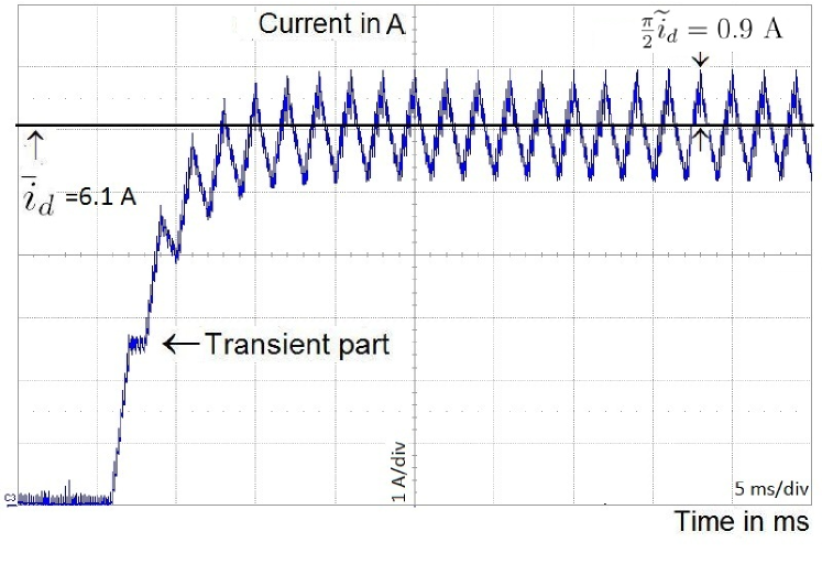
Figure 1: Experimental time response of idsubscript𝑖𝑑i_{d} in (31)-(32)

IV Estimation of magnetic parameters

The seven parameters in the saturation model (7)-(8) must of course be estimated. This can be done with a rather simple procedure also relying on signal injection and averaging.

IV-A Principle

The rotor is locked in the position θ:=0assign𝜃0\theta:=0, hence the model (1)–(3) reduces to ω=0𝜔0\omega=0 and

dϕdqdt𝑑subscriptitalic-ϕ𝑑𝑞𝑑𝑡\displaystyle\frac{d\phi_{dq}}{dt} =\displaystyle= udqRidq,subscript𝑢𝑑𝑞𝑅subscript𝑖𝑑𝑞\displaystyle u_{dq}-Ri_{dq}, (31)

with idq=dq(ϕdq)subscript𝑖𝑑𝑞subscript𝑑𝑞subscriptitalic-ϕ𝑑𝑞i_{dq}=\mathcal{I}_{dq}(\phi_{dq}). Moreover udqsubscript𝑢𝑑𝑞u_{dq} can now be physically impressed and idqsubscript𝑖𝑑𝑞i_{dq} physically measured.

As in section III-A, but now working directly in the dq𝑑𝑞d-q frame, we inject a fast-varying pulsating voltage

udqsubscript𝑢𝑑𝑞\displaystyle u_{dq} =\displaystyle= u¯dq+u~dqf(Ωt),subscript¯𝑢𝑑𝑞subscript~𝑢𝑑𝑞𝑓Ω𝑡\displaystyle\overline{u}_{dq}+\widetilde{u}_{dq}f({\Omega}t), (32)

with constant u¯dqsubscript¯𝑢𝑑𝑞\overline{u}_{dq} and u~dqsubscript~𝑢𝑑𝑞\widetilde{u}_{dq}. The solution of (31)-(32) is then

ϕdqsubscriptitalic-ϕ𝑑𝑞\displaystyle\phi_{dq} =\displaystyle= ϕ¯dq+u~dqΩF(Ωt)+𝒪(1Ω2)subscript¯italic-ϕ𝑑𝑞subscript~𝑢𝑑𝑞Ω𝐹Ω𝑡𝒪1superscriptΩ2\displaystyle\overline{\phi}_{dq}+\frac{\widetilde{u}_{dq}}{\Omega}F(\Omega t)+{\mathcal{O}}(\frac{1}{\Omega^{2}})

where ϕ¯dqsubscript¯italic-ϕ𝑑𝑞\overline{\phi}_{dq}, the “slowly-varying” component of ϕdqsubscriptitalic-ϕ𝑑𝑞\phi_{dq}, satisfies

dϕ¯dqdt𝑑subscript¯italic-ϕ𝑑𝑞𝑑𝑡\displaystyle\frac{d\overline{\phi}_{dq}}{dt} =\displaystyle= u¯dRi¯d,subscript¯𝑢𝑑𝑅subscript¯𝑖𝑑\displaystyle\overline{u}_{d}-R\overline{i}_{d}, (33)

with i¯dq=dq(ϕ¯dq)subscript¯𝑖𝑑𝑞subscript𝑑𝑞subscript¯italic-ϕ𝑑𝑞\overline{i}_{dq}=\mathcal{I}_{dq}(\overline{\phi}_{dq}). Moreover (29) now boils down to

i~dqsubscript~𝑖𝑑𝑞\displaystyle\widetilde{i}_{dq} =\displaystyle= Ddq(dq1(i¯dq))u~dqΩ.𝐷subscript𝑑𝑞superscriptsubscript𝑑𝑞1subscript¯𝑖𝑑𝑞subscript~𝑢𝑑𝑞Ω\displaystyle D\mathcal{I}_{dq}\bigl{(}\mathcal{I}_{dq}^{-1}(\overline{i}_{dq})\bigr{)}\frac{\widetilde{u}_{dq}}{\Omega}. (34)

Since u¯dqsubscript¯𝑢𝑑𝑞\overline{u}_{dq} is constant (33) implies Ri¯dq𝑅subscript¯𝑖𝑑𝑞R\overline{i}_{dq} tends to u¯dqsubscript¯𝑢𝑑𝑞\overline{u}_{dq}, hence after an initial transient i¯dqsubscript¯𝑖𝑑𝑞\overline{i}_{dq} is constant. As a consequence i~dqsubscript~𝑖𝑑𝑞\widetilde{i}_{dq} is by (34) also constant. Fig. 1 shows for instance the time response of idsubscript𝑖𝑑i_{d} for the SPM motor of section IV-C starting from id(0)=0subscript𝑖𝑑00i_{d}(0)=0 and using a square function f𝑓f; notice the current ripples seen on the scope are maxτ[0,2π]F(τ)=π2subscript𝜏02𝜋𝐹𝜏𝜋2\max_{\tau\in[0,2\pi]}F(\tau)=\frac{\pi}{2} (since f𝑓f is square with period 2π2𝜋2\pi) smaller than i~dqsubscript~𝑖𝑑𝑞\widetilde{i}_{dq}.

The magnetic parameters can then be estimated repeatedly using (34) with various values of u¯dqsubscript¯𝑢𝑑𝑞\overline{u}_{dq} and u~dqsubscript~𝑢𝑑𝑞\widetilde{u}_{dq}, as detailed in the next section.

TABLE I: Rated and estimated magnetic parameters of test motors
Motor IPM SPM
Rated power 750 W 1500 W
Rated current Insubscript𝐼𝑛I_{n} (peak) 4.51 A 5.19 A
Rated voltage (peak per phase) 110 V 245 V
Rated speed 1800 rpm 3000 rpm
Rated torque 3.98 Nm 6.06 Nm
n𝑛n 3 5
R𝑅R 1.52Ω1.52Ω1.52~{}{\Omega} 2.1Ω2.1Ω2.1~{}{\Omega}
λ𝜆\lambda (peak) 196196196 mWb 155155155 mWb
Ldsubscript𝐿𝑑L_{d} 9.159.159.15 mH 7.867.867.86 mH
Lqsubscript𝐿𝑞L_{q} 13.5813.5813.58 mH 8.188.188.18 mH
α3,0Ld2Insubscript𝛼30superscriptsubscript𝐿𝑑2subscript𝐼𝑛\alpha_{3,0}L_{d}^{2}I_{n} 0.0390.0390.039 0.0560.0560.056
α1,2LdLqInsubscript𝛼12subscript𝐿𝑑subscript𝐿𝑞subscript𝐼𝑛\alpha_{1,2}L_{d}L_{q}I_{n} 0.0530.0530.053 0.0550.0550.055
α4,0Ld3In2subscript𝛼40superscriptsubscript𝐿𝑑3superscriptsubscript𝐼𝑛2\alpha_{4,0}L_{d}^{3}I_{n}^{2} 0.00510.00510.0051 0.01640.01640.0164
α2,2LdLq2In2subscript𝛼22subscript𝐿𝑑superscriptsubscript𝐿𝑞2superscriptsubscript𝐼𝑛2\alpha_{2,2}L_{d}L_{q}^{2}I_{n}^{2} 0.01710.01710.0171 0.0270.0270.027
α0,4Lq3In2subscript𝛼04superscriptsubscript𝐿𝑞3superscriptsubscript𝐼𝑛2\alpha_{0,4}L_{q}^{3}I_{n}^{2} 0.00600.00600.0060 0.00670.00670.0067
Refer to caption
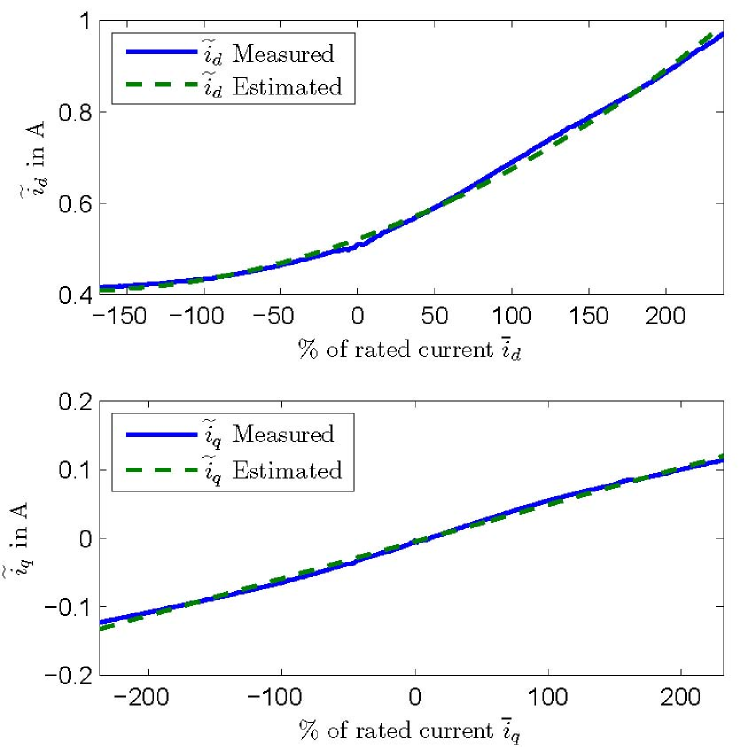
Figure 2: IPM: fitted values vs measurements for (37) and (39)
Refer to caption
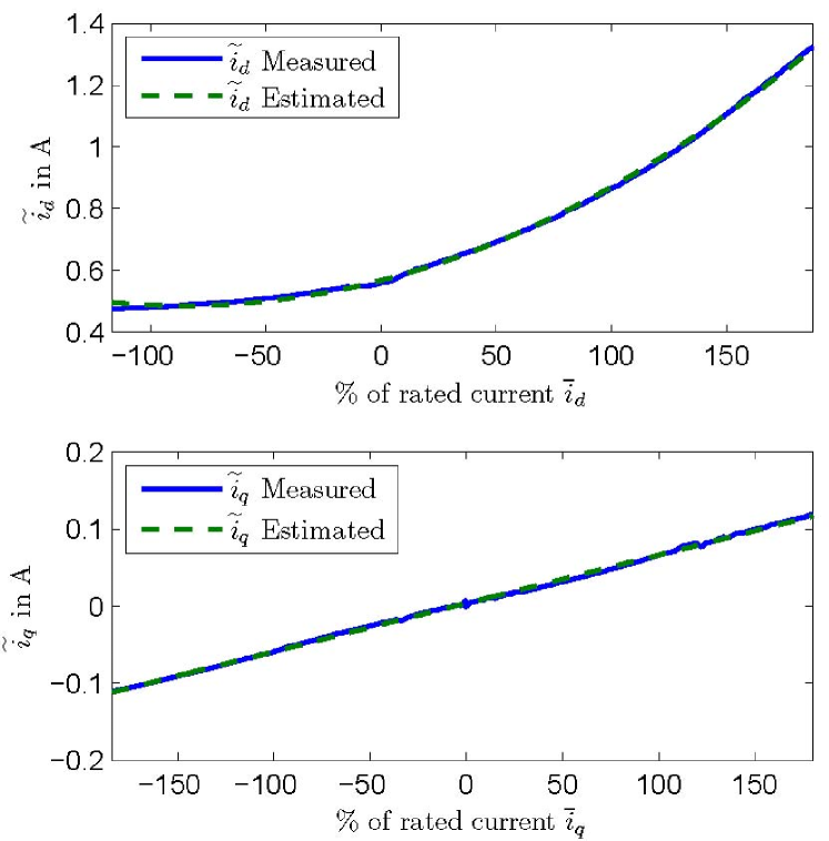
Figure 3: SPM: fitted values vs measurements for (37) and (39)

IV-B Estimation of the parameters

From (11) the entries of Ddq(dq1(i¯dq))𝐷subscript𝑑𝑞superscriptsubscript𝑑𝑞1subscript¯𝑖𝑑𝑞D\mathcal{I}_{dq}\bigl{(}\mathcal{I}_{dq}^{-1}(\overline{i}_{dq})\bigr{)} are given by

Gdd(i¯dq)subscript𝐺𝑑𝑑subscript¯𝑖𝑑𝑞\displaystyle G_{dd}(\overline{i}_{dq}) =1Ld+6α3,0Ldi¯d+12α4,0Ld2i¯d2+2α2,2Lq2i¯q2absent1subscript𝐿𝑑6subscript𝛼30subscript𝐿𝑑subscript¯𝑖𝑑12subscript𝛼40superscriptsubscript𝐿𝑑2superscriptsubscript¯𝑖𝑑22subscript𝛼22superscriptsubscript𝐿𝑞2superscriptsubscript¯𝑖𝑞2\displaystyle=\frac{1}{L_{d}}+6\alpha_{3,0}L_{d}\overline{i}_{d}+12\alpha_{4,0}L_{d}^{2}\overline{i}_{d}^{2}+2\alpha_{2,2}L_{q}^{2}\overline{i}_{q}^{2}
Gdq(i¯dq)subscript𝐺𝑑𝑞subscript¯𝑖𝑑𝑞\displaystyle G_{dq}(\overline{i}_{dq}) =2α1,2Lqi¯q+4α2,2Ldi¯dLqi¯qabsent2subscript𝛼12subscript𝐿𝑞subscript¯𝑖𝑞4subscript𝛼22subscript𝐿𝑑subscript¯𝑖𝑑subscript𝐿𝑞subscript¯𝑖𝑞\displaystyle=2\alpha_{1,2}L_{q}\overline{i}_{q}+4\alpha_{2,2}L_{d}\overline{i}_{d}L_{q}\overline{i}_{q}
Gqq(i¯dq)subscript𝐺𝑞𝑞subscript¯𝑖𝑑𝑞\displaystyle G_{qq}(\overline{i}_{dq}) =1Lq+2α1,2Ldi¯d+2α2,2Ld2i¯d2+12α0,4Lq2i¯q2.absent1subscript𝐿𝑞2subscript𝛼12subscript𝐿𝑑subscript¯𝑖𝑑2subscript𝛼22superscriptsubscript𝐿𝑑2superscriptsubscript¯𝑖𝑑212subscript𝛼04superscriptsubscript𝐿𝑞2superscriptsubscript¯𝑖𝑞2\displaystyle=\frac{1}{L_{q}}+2\alpha_{1,2}L_{d}\overline{i}_{d}+2\alpha_{2,2}L_{d}^{2}\overline{i}_{d}^{2}+12\alpha_{0,4}L_{q}^{2}\overline{i}_{q}^{2}.

Since combinations of the magnetic parameters always enter linearly those equations, they can be estimated by simple linear least squares; moreover by suitably choosing u¯dqsubscript¯𝑢𝑑𝑞\overline{u}_{dq} and u~dqsubscript~𝑢𝑑𝑞\widetilde{u}_{dq}, the whole least squares problem for the seven parameters can be split into several subproblems involving fewer parameters:

  • with u¯dq:=0assignsubscript¯𝑢𝑑𝑞0\overline{u}_{dq}:=0, hence i¯dq=0subscript¯𝑖𝑑𝑞0\overline{i}_{dq}=0, (34) reads

    Ldsubscript𝐿𝑑\displaystyle L_{d} =\displaystyle= 1Ωu~di~d1Ωsubscript~𝑢𝑑subscript~𝑖𝑑\displaystyle\frac{1}{{\Omega}}\frac{\widetilde{u}_{d}}{\widetilde{i}_{d}} (35)
    Lqsubscript𝐿𝑞\displaystyle L_{q} =\displaystyle= 1Ωu~qi~q1Ωsubscript~𝑢𝑞subscript~𝑖𝑞\displaystyle\frac{1}{{\Omega}}\frac{\widetilde{u}_{q}}{\widetilde{i}_{q}} (36)
  • with u¯q=0subscript¯𝑢𝑞0\overline{u}_{q}=0, hence i¯q=0subscript¯𝑖𝑞0\overline{i}_{q}=0, and u~q=0subscript~𝑢𝑞0\widetilde{u}_{q}=0 (34) reads

    i~dsubscript~𝑖𝑑\displaystyle\widetilde{i}_{d} =\displaystyle= u~dΩ(1Ld+6α3,0Ldi¯d+12α4,0Ld2i¯d2)subscript~𝑢𝑑Ω1subscript𝐿𝑑6subscript𝛼30subscript𝐿𝑑subscript¯𝑖𝑑12subscript𝛼40superscriptsubscript𝐿𝑑2superscriptsubscript¯𝑖𝑑2\displaystyle\frac{\widetilde{u}_{d}}{{\Omega}}\left(\frac{1}{L_{d}}+6\alpha_{3,0}L_{d}\overline{i}_{d}+12\alpha_{4,0}L_{d}^{2}\overline{i}_{d}^{2}\right) (37)
    i~qsubscript~𝑖𝑞\displaystyle\widetilde{i}_{q} =\displaystyle= 00\displaystyle 0
  • with u¯d=0subscript¯𝑢𝑑0\overline{u}_{d}=0, hence i¯d:=0assignsubscript¯𝑖𝑑0\overline{i}_{d}:=0, and u~q=0subscript~𝑢𝑞0\widetilde{u}_{q}=0 (34) reads

    i~dsubscript~𝑖𝑑\displaystyle\widetilde{i}_{d} =u~dΩ(1Ld+2α2,2Lq2i¯q2)absentsubscript~𝑢𝑑Ω1subscript𝐿𝑑2subscript𝛼22superscriptsubscript𝐿𝑞2superscriptsubscript¯𝑖𝑞2\displaystyle=\frac{\widetilde{u}_{d}}{{\Omega}}\Bigl{(}\frac{1}{L_{d}}+2\alpha_{2,2}L_{q}^{2}\overline{i}_{q}^{2}\Bigr{)} (38)
    i~qsubscript~𝑖𝑞\displaystyle\widetilde{i}_{q} =2u~dΩα1,2Lqi¯qabsent2subscript~𝑢𝑑Ωsubscript𝛼12subscript𝐿𝑞subscript¯𝑖𝑞\displaystyle=\frac{2\widetilde{u}_{d}}{{\Omega}}\alpha_{1,2}L_{q}\overline{i}_{q} (39)
  • with u¯d=0subscript¯𝑢𝑑0\overline{u}_{d}=0, hence i¯d:=0assignsubscript¯𝑖𝑑0\overline{i}_{d}:=0, and u~d=0subscript~𝑢𝑑0\widetilde{u}_{d}=0 (34) reads

    i~dsubscript~𝑖𝑑\displaystyle\widetilde{i}_{d} =2u~qΩα1,2Lqi¯qabsent2subscript~𝑢𝑞Ωsubscript𝛼12subscript𝐿𝑞subscript¯𝑖𝑞\displaystyle=\frac{2\widetilde{u}_{q}}{{\Omega}}\alpha_{1,2}L_{q}\overline{i}_{q} (40)
    i~qsubscript~𝑖𝑞\displaystyle\widetilde{i}_{q} =u~qΩ(1Lq+12α0,4Lq2i¯q2).absentsubscript~𝑢𝑞Ω1subscript𝐿𝑞12subscript𝛼04superscriptsubscript𝐿𝑞2superscriptsubscript¯𝑖𝑞2\displaystyle=\frac{\widetilde{u}_{q}}{{\Omega}}\Bigl{(}\frac{1}{L_{q}}+12\alpha_{0,4}L_{q}^{2}\overline{i}_{q}^{2}\Bigr{)}. (41)

Ldsubscript𝐿𝑑L_{d} and Lqsubscript𝐿𝑞L_{q} are then immediately determined from (35) and (36); α3,0subscript𝛼30\alpha_{3,0} and α4,0subscript𝛼40\alpha_{4,0} are jointly estimated by least squares from (37); α2,2subscript𝛼22\alpha_{2,2}, α1,2subscript𝛼12\alpha_{1,2} and α0,4subscript𝛼04\alpha_{0,4} are separately estimated by least squares from respectively (38), (39)-(40) and (41).
Refer to caption
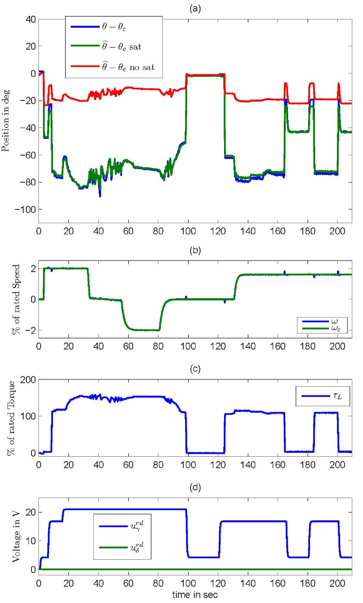
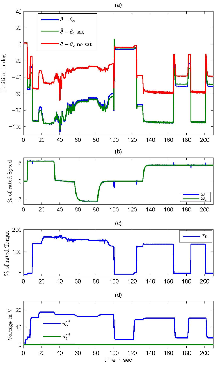
Figure 4: Long test under various conditions for IPM: (a) measured θθc𝜃subscript𝜃𝑐\theta-\theta_{c}, estimated θ^θc^𝜃subscript𝜃𝑐\widehat{\theta}-\theta_{c} with and without saturation model; (b) measured speed ω𝜔\omega, reference speed ωcsubscript𝜔𝑐\omega_{c}; (c) load torque τLsubscript𝜏𝐿\tau_{L}; (d) voltages uγδrdsuperscriptsubscript𝑢𝛾𝛿𝑟𝑑u_{\gamma\delta}^{rd}
Refer to caption
Figure 5: Long test under various conditions for SPM: (a) measured θθc𝜃subscript𝜃𝑐\theta-\theta_{c}, estimated θ^θc^𝜃subscript𝜃𝑐\widehat{\theta}-\theta_{c} with and without saturation model; (b) measured speed ω𝜔\omega, reference speed ωcsubscript𝜔𝑐\omega_{c}; (c) load torque τLsubscript𝜏𝐿\tau_{L}; (d) voltages uγδrdsuperscriptsubscript𝑢𝛾𝛿𝑟𝑑u_{\gamma\delta}^{rd}

IV-C Experimental setup

The methodology developed in the paper was tested on two types of motors, an Interior Magnet PMSM (IPM) and a Surface-Mounted PMSM (SPM), with rated parameters listed in the top part of table I.

The experimental setup consists of an industrial inverter (400400400 V DC bus, 444 kHz PWM frequency), an incremental encoder, a dSpace fast prototyping system with 3 boards (DS1005, DS5202 and EV1048), and a host PC. The measurements are sampled also at 444 kHz, and synchronized with the PWM frequency. The load torque is created by a 444 kW DC motor.

IV-D Estimation of the magnetic parameters

We follow the procedure described in section IV: with the rotor locked in the position θ:=0assign𝜃0\theta:=0, a square wave voltage with frequency Ω:=2π×500rad/sassignΩ2𝜋500rad/s\Omega:=2\pi\times 500\,\text{rad/s} and constant amplitude u~dsubscript~𝑢𝑑\widetilde{u}_{d} or u~qsubscript~𝑢𝑞\widetilde{u}_{q} (15 V for the IPM, 141414 V for the SPM) is applied to the motor; but for the determination of Ld,Lqsubscript𝐿𝑑subscript𝐿𝑞L_{d},L_{q} where u¯d=u¯q:=0subscript¯𝑢𝑑subscript¯𝑢𝑞assign0\overline{u}_{d}=\overline{u}_{q}:=0, several runs are performed with various u¯dsubscript¯𝑢𝑑\overline{u}_{d} (resp. u¯qsubscript¯𝑢𝑞\overline{u}_{q}) such that i¯dsubscript¯𝑖𝑑\overline{i}_{d} (resp. i¯qsubscript¯𝑖𝑞\overline{i}_{q}) ranges from 200%percent200-200\% to +200%percent200+200\% of the rated current. The magnetic parameters are then estimated by linear least squares according to section IV-B, yielding the values in the bottom part of table I. Notice the SPM exhibits as expected little geometric saliency (LdLqsubscript𝐿𝑑subscript𝐿𝑞L_{d}\approx L_{q}) hence the saturation-induced saliency is paramount to estimate the rotor position. Notice also the cross-saturation term α12subscript𝛼12\alpha_{12} is as expected quantitatively important for both motors.

The good agreement between the fitted curves and the measurements is demonstrated for instance for (37) and (39) on Fig. 2-3; notice (37) corresponds to saturation on a single axis while (39) corresponds to cross-saturation.
Refer to caption
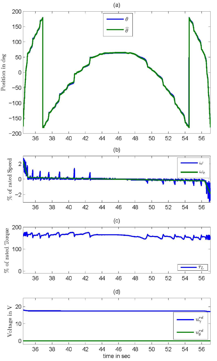
Figure 6: Slow speed reversal for IPM: (a) measured θ𝜃\theta, estimated θ^^𝜃\widehat{\theta}; (b) measured speed ω𝜔\omega, reference speed ωcsubscript𝜔𝑐\omega_{c}; (c) load torque τLsubscript𝜏𝐿\tau_{L}; (d) voltages uγδrdsuperscriptsubscript𝑢𝛾𝛿𝑟𝑑u_{\gamma\delta}^{rd}
Refer to caption
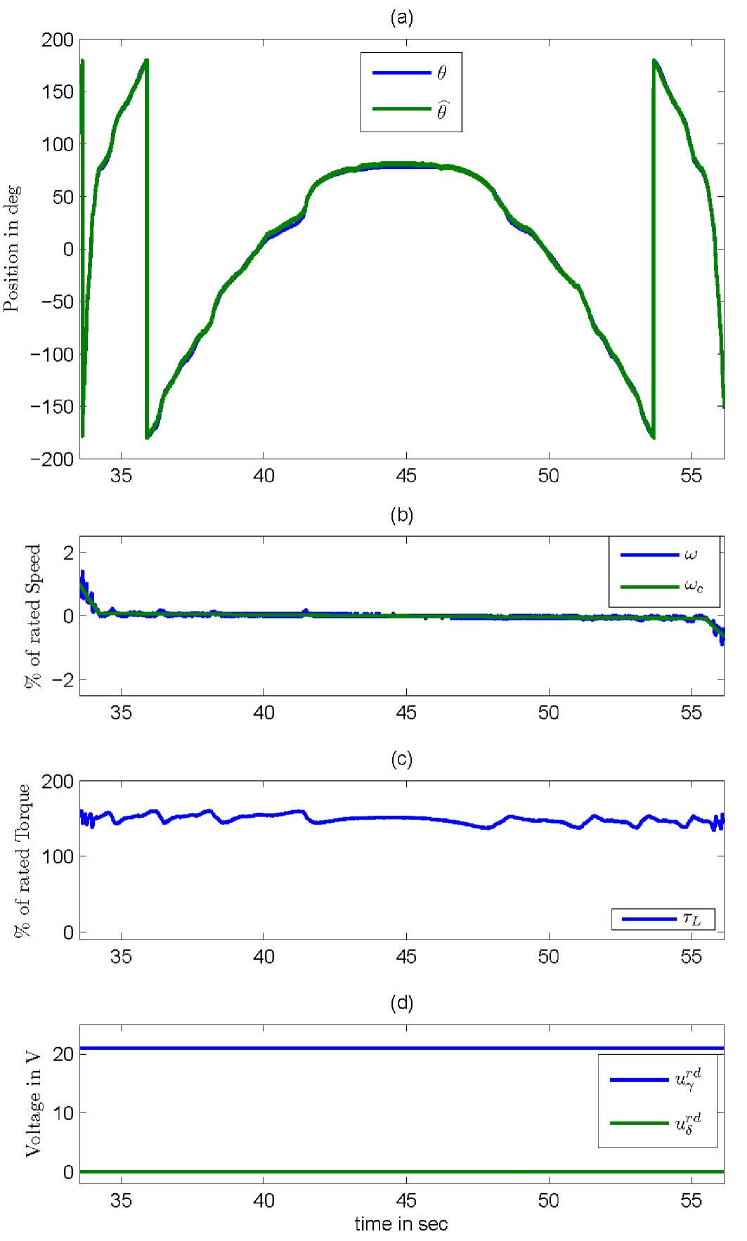
Figure 7: Slow speed reversal for SPM: (a) measured θ𝜃\theta, estimated θ^^𝜃\widehat{\theta}; (b) measured speed ω𝜔\omega, reference speed ωcsubscript𝜔𝑐\omega_{c}; (c) load torque τLsubscript𝜏𝐿\tau_{L}; (d) voltages uγδrdsuperscriptsubscript𝑢𝛾𝛿𝑟𝑑u_{\gamma\delta}^{rd}

IV-E Validation of the rotor position estimation procedure

The relevance of the position estimation methodology developed in section  III is now illustrated on the two test motors, using the parameters estimated in the previous section. Since the goal is only to test the validity of the angle estimation procedure, a very simple V/f𝑉𝑓V/f open-loop (i.e. ΩcsubscriptΩ𝑐\Omega_{c} and 𝒰γδsubscript𝒰𝛾𝛿\mathcal{U}_{\gamma\delta} do not depend on iγδsubscript𝑖𝛾𝛿i_{\gamma\delta}) control law is used for (12)–(16); a fast-varying (Ω:=2π×500rad/sassignΩ2𝜋500rad/s\Omega:=2\pi\times 500\,\text{rad/s}) square voltage with constant amplitude is added in accordance with (21), resulting in

dθcdt𝑑subscript𝜃𝑐𝑑𝑡\displaystyle\frac{d\theta_{c}}{dt} =ωc(t)absentsubscript𝜔𝑐𝑡\displaystyle={\omega}_{c}(t)
uγδsubscript𝑢𝛾𝛿\displaystyle u_{\gamma\delta} =uγδrd(t)+ωc(t)ϕm+u~γδf(Ωt).absentsuperscriptsubscript𝑢𝛾𝛿𝑟𝑑𝑡subscript𝜔𝑐𝑡subscriptitalic-ϕ𝑚subscript~𝑢𝛾𝛿𝑓Ω𝑡\displaystyle=u_{\gamma\delta}^{rd}(t)+{\omega}_{c}(t)\phi_{m}+\widetilde{u}_{\gamma\delta}f(\Omega t).

Here ωc(t)subscript𝜔𝑐𝑡{\omega}_{c}(t) is the motor speed reference; uγδrd(t)superscriptsubscript𝑢𝛾𝛿𝑟𝑑𝑡u_{\gamma\delta}^{rd}(t) is a filtered piece-wise constant vector compensating the resistive voltage drop in order to maintain the torque level and the motor stability; finally u~γδ:=(u~,0)Tassignsubscript~𝑢𝛾𝛿superscript~𝑢0𝑇\widetilde{u}_{\gamma\delta}:=(\widetilde{u},0)^{T} with u~:=15assign~𝑢15\widetilde{u}:=15 V.

The rotor position θ^^𝜃\widehat{\theta} is then estimated according to (30).

IV-E1 Long test under various conditions, Fig. 4-5

Speed and torque are changed over a period of 210210210 seconds; the speed remains between ±5%plus-or-minuspercent5\pm 5\% of the rated speed and the torque varies from 0%percent00\% to 180%percent180180\% of the rated toque. This represents typical operation conditions at low speed.

When the saturation model is used the agreement between the estimated position θ^^𝜃\widehat{\theta} and the measured position θ𝜃\theta is very good, with an error always smaller than a few (electrical) degrees. By contrast the estimated error without using the saturation model (i.e. with all the magnetic saturation parameters αijsubscript𝛼𝑖𝑗\alpha_{ij} taken to zero) can reach up to 40superscript4040^{\circ} for the IPM and 70superscript7070^{\circ} the SPM. This demonstrates the importance of considering an adequate saturation model including in particular cross-saturation.

IV-E2 Slow speed reversal, Fig. 6-7

This is an excerpt of the long experiment between 353535 s and 555555 s. The speed is slowly changed from 0.2%percent0.2-0.2\% to +0.2%percent0.2+0.2\% of the rated speed at 150%percent150150\% of the rated torque. This is a very demanding test since the motor always remains in the poor observability region, moreover under high load. Once again the estimated angle closely agrees with the measured angle.

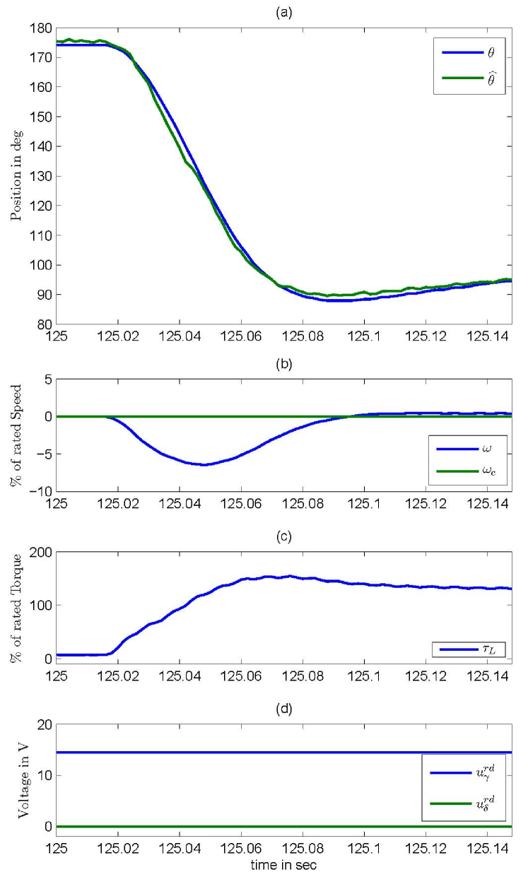
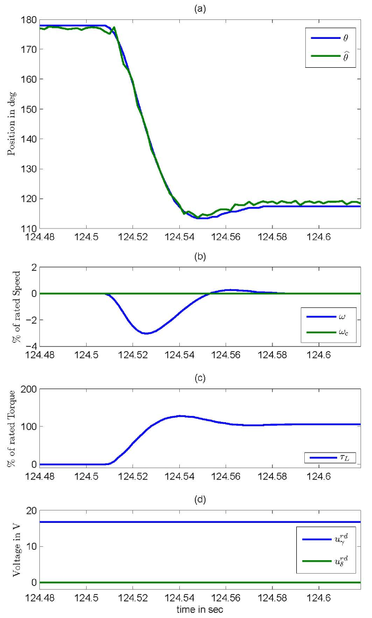
IV-E3 Load step at zero speed, Fig. 8-9

This is an excerpt of the long experiment around t=125𝑡125t=125 s. The load is suddenly changed from 0%percent00\% to 100%percent100100\% of the rated torque while the motor is at rest. This test illustrates the quality of the estimation also under dynamic conditions.
Refer to caption
Figure 8: Load step at zero speed for IPM: (a) measured θ𝜃\theta, estimated θ^^𝜃\widehat{\theta}; (b) measured speed ω𝜔\omega, reference speed ωcsubscript𝜔𝑐\omega_{c}; (c) load torque τLsubscript𝜏𝐿\tau_{L}; (d) voltages uγδrdsuperscriptsubscript𝑢𝛾𝛿𝑟𝑑u_{\gamma\delta}^{rd}
Refer to caption
Figure 9: Load step at zero speed for SPM: (a) measured θ𝜃\theta, estimated θ^^𝜃\widehat{\theta}; (b) measured speed ω𝜔\omega, reference speed ωcsubscript𝜔𝑐\omega_{c}; (c) load torque τLsubscript𝜏𝐿\tau_{L}; (d) voltages uγδrdsuperscriptsubscript𝑢𝛾𝛿𝑟𝑑u_{\gamma\delta}^{rd}

V Conclusion

We have presented a simple parametric model of the saturated PMSM together with a new procedure based on signal injection for estimating the rotor angle at low speed relying on an original analysis based on second-order averaging. This is not an easy problem in view of the observability degeneracy at zero speed. The method is general in the sense it can accommodate virtually any control law, saturation model, and form of injected signal. The relevance of the method and the importance of using an adequate magnetic saturation model has been experimentally demonstrated on a SPM motor with little geometric saliency as well as on an IPM motor.

References

  • [1] P. Jansen and R. Lorenz, “Transducerless position and velocity estimation in induction and salient AC machines,” IEEE Trans. Industry Applications, vol. 31, pp. 240–247, 1995.
  • [2] S. Ogasawara and H. Akagi, “An approach to real-time position estimation at zero and low speed for a PM motor based on saliency,” IEEE Trans. Industry Applications, vol. 34, pp. 163–168, 1998.
  • [3] M. Corley and R. Lorenz, “Rotor position and velocity estimation for a salient-pole permanent magnet synchronous machine at standstill and high speeds,” IEEE Trans. Industry Applications, vol. 34, pp. 784–789, 1998.
  • [4] T. Aihara, A. Toba, T. Yanase, A. Mashimo, and K. Endo, “Sensorless torque control of salient-pole synchronous motor at zero-speed operation,” IEEE Trans. Power Electronics, vol. 14, pp. 202–208, 1999.
  • [5] A. Consoli, G. Scarcella, and A. Testa, “Industry application of zero-speed sensorless control techniques for PM synchronous motors,” IEEE Trans. Industry Applications, vol. 37, no. 2, pp. 513–521, 2001.
  • [6] J.-I. Ha, K. Ide, T. Sawa, and S.-K. Sul, “Sensorless rotor position estimation of an interior permanent-magnet motor from initial states,” IEEE Trans. Industry Applications, vol. 39, no. 3, pp. 761–767, 2003.
  • [7] J.-H. Jang, S.-K. Sul, J.-I. Ha, K. Ide, and M. Sawamura, “Sensorless drive of surface-mounted permanent-magnet motor by high-frequency signal injection based on magnetic saliency,” IEEE Trans. Industry Applications, vol. 39, pp. 1031–1039, 2003.
  • [8] J.-H. Jang, J.-I. Ha, M. Ohto, K. Ide, and S.-K. Sul, “Analysis of permanent-magnet machine for sensorless control based on high-frequency signal injection,” IEEE Trans. Industry Applications, vol. 40, no. 6, pp. 1595–1604, 2004.
  • [9] E. Robeischl and M. Schroedl, “Optimized INFORM measurement sequence for sensorless PM synchronous motor drives with respect to minimum current distortion,” IEEE Trans. Industry Applications, vol. 40, no. 2, pp. 591–598, 2004.
  • [10] S. Shinnaka, “A new speed-varying ellipse voltage injection method for sensorless drive of permanent-magnet synchronous motors with pole saliency - New PLL method using high-frequency current component multiplied signal,” IEEE Trans. Industry Applications, vol. 44, no. 3, pp. 777–788, 2008.
  • [11] L. Harnefors and H.-P. Nee, “A general algorithm for speed and position estimation of AC motors,” IEEE Trans. Industrial Electronics, vol. 47, no. 1, pp. 77–83, 2000.
  • [12] O. Wallmark, L. Harnefors, and O. Carlson, “An improved speed and position estimator for salient permanent-magnet synchronous motors,” IEEE Trans. Industrial Electronics, vol. 52, no. 1, pp. 255–262, 2005.
  • [13] C. Silva, G. Asher, and M. Sumner, “Hybrid rotor position observer for wide speed-range sensorless PM motor drives including zero speed,” IEEE Trans. Industrial Electronics, vol. 53, no. 2, pp. 373–378, 2006.
  • [14] A. Piippo, M. Hinkkanen, and J. Luomi, “Analysis of an adaptive observer for sensorless control of interior permanent magnet synchronous motors,” IEEE Trans. Industrial Electronics, vol. 55, no. 2, pp. 570–576, 2008.
  • [15] G. Foo and M. Rahman, “Sensorless sliding-mode MTPA control of an IPM synchronous motor drive using a sliding-mode observer and HF signal injection,” IEEE Trans. Industrial Electronics, vol. 57, no. 4, pp. 1270–1278, 2010.
  • [16] P. Guglielmi, M. Pastorelli, and A. Vagati, “Cross-saturation effects in IPM motors and related impact on sensorless control,” IEEE Trans. Industry Applications, vol. 42, pp. 1516–1522, 2006.
  • [17] N. Bianchi, S. Bolognani, J.-H. Jang, and S.-K. Sul, “Comparison of PM motor structures and sensorless control techniques for zero-speed rotor position detection,” IEEE Trans. Power Electronics, vol. 22, no. 6, pp. 2466–2475, 2007.
  • [18] J. Holtz, “Acquisition of position error and magnet polarity for sensorless control of PM synchronous machines,” IEEE Trans. Industry Applications, vol. 44, no. 4, pp. 1172–1180, 2008.
  • [19] D. Reigosa, P. García, D. Raca, F. Briz, and R. Lorenz, “Measurement and adaptive decoupling of cross-saturation effects and secondary saliencies in sensorless controlled IPM synchronous machines,” IEEE Trans. Industry Applications, vol. 44, no. 6, pp. 1758–1767, 2008.
  • [20] N. Bianchi, S. Bolognani, and A. Faggion, “Predicted and measured errors in estimating rotor position by signal injection for salient-pole PM synchronous motors,” in IEEE International Electric Machines and Drives Conference, 2009, pp. 1565–1572.
  • [21] H. De Kock, M. Kamper, and R. Kennel, “Anisotropy comparison of reluctance and PM synchronous machines for position sensorless control using HF carrier injection,” IEEE Trans. Power Electronics, vol. 24, no. 8, pp. 1905–1913, 2009.
  • [22] Y. Li, Z. Zhu, D. Howe, C. Bingham, and D. Stone, “Improved rotor-position estimation by signal injection in brushless AC motors, accounting for cross-coupling magnetic saturation,” IEEE Trans. Industry Applications, vol. 45, pp. 1843–1850, 2009.
  • [23] P. Sergeant, F. De Belie, and J. Melkebeek, “Effect of rotor geometry and magnetic saturation in sensorless control of PM synchronous machines,” IEEE Trans. Magnetics, vol. 45, no. 3, pp. 1756–1759, 2009.
  • [24] D. Raca, P. García, D. Reigosa, F. Briz, and R. Lorenz, “Carrier-signal selection for sensorless control of PM synchronous machines at zero and very low speeds,” IEEE Trans. Industry Applications, vol. 46, no. 1, pp. 167–178, 2010.
  • [25] N. Bianchi, E. Fornasiero, and S. Bolognani, “Effect of stator and rotor saturation on sensorless rotor position detection,” in IEEE Energy Conversion Congress and Exposition, 2011, pp. 1528–1535.
  • [26] Z. Zhu and L. Gong, “Investigation of effectiveness of sensorless operation in carrier-signal-injection-based sensorless-control methods,” IEEE Trans. Industrial Electronics, vol. 58, no. 8, pp. 3431–3439, 2011.
  • [27] F. Parasiliti and P. Poffet, “Model for saturation effects in high-field permanent magnet synchronous motors,” IEEE Trans. Energy Conversion, vol. 4, no. 3, pp. 487–494, 1989.
  • [28] M. Cheng, K. Chau, and C. Chan, “Nonlinear varying-network magnetic circuit analysis for doubly salient permanent-magnet motors,” IEEE Trans. Magnetics, vol. 36, no. 1 PART 2, pp. 339–348, 2000.
  • [29] B. Štumberger, G. Štumberger, D. Dolinar, A. Hamler, and M. Trlep, “Evaluation of saturation and cross-magnetization effects in interior permanent-magnet synchronous motor,” IEEE Trans. Industry Applications, vol. 39, no. 5, pp. 1264–1271, 2003.
  • [30] K. Rahman and S. Hiti, “Identification of machine parameters of a synchronous motor,” IEEE Trans. Industry Applications, vol. 41, no. 2, pp. 557–565, 2005.
  • [31] G. Štumberger, B. Štumberger, B. Štumberger, M. Toman, and D. Dolinar, “Evaluation of experimental methods for determining the magnetically nonlinear characteristics of electromagnetic devices,” IEEE Trans. Magnetics, vol. 41, no. 10, pp. 4030–4032, 2005.
  • [32] E. Armando, P. Guglielmi, G. Pellegrino, M. Pastorelli, and A. Vagati, “Accurate modeling and performance analysis of IPM-PMASR motors,” IEEE Trans. Industry Applications, vol. 45, no. 1, pp. 123–130, 2009.
  • [33] A. Jebai, F. Malrait, P. Martin, and P. Rouchon, “Estimation of saturation of permanent-magnet synchronous motors through an energy-based model,” in IEEE International Electric Machines Drives Conference, 2011, pp. 1316 –1321.
  • [34] Y.-D. Yoon, S.-K. Sul, S. Morimoto, and K. Ide, “High-bandwidth sensorless algorithm for AC machines based on square-wave-type voltage injection,” IEEE Trans. Industry Applications, vol. 47, no. 3, pp. 1361–1370, 2011.
  • [35] D. Basic, F. Malrait, and P. Rouchon, “Euler-Lagrange models with complex currents of three-phase electrical machines and observability issues,” IEEE Trans. Automatic Control, vol. 55, pp. 212–217, 2010.
  • [36] D. Basic, A. K. Jebai, F. Malrait, P. Martin, and P. Rouchon, “Using Hamiltonians to model saturation in space vector representations of AC electrical machines,” in Advances in the theory of control, signals and systems with physical modeling, ser. Lecture Notes in Control and Information Sciences, J. Lévine and P. Müllhaupt, Eds.   Springer, 2011, pp. 41–48.
  • [37] J. A. Sanders, F. Verhulst, and J. Murdock, Averaging methods in nonlinear dynamical systems, 2nd ed., ser. Applied Mathematical Sciences.   Springer, 2007, no. 59.