Measuring the Irreversibility of Numerical Schemes for Reversible Stochastic Differential Equations

Abstract.

For a stationary Markov process the detailed balance condition is equivalent to the time-reversibility of the process. For stochastic differential equations (SDE’s), the time discretization of numerical schemes usually destroys the time-reversibility property. Despite an extensive literature on the numerical analysis for SDE’s, their stability properties, strong and/or weak error estimates, large deviations and infinite-time estimates, no quantitative results are known on the lack of reversibility of discrete-time approximation processes. In this paper we provide such quantitative estimates by using the concept of entropy production rate, inspired by ideas from non-equilibrium statistical mechanics. The entropy production rate for a stochastic process is defined as the relative entropy (per unit time) of the path measure of the process with respect to the path measure of the time-reversed process. By construction the entropy production rate is nonnegative and it vanishes if and only if the process is reversible. Crucially, from a numerical point of view, the entropy production rate is an a posteriori quantity, hence it can be computed in the course of a simulation as the ergodic average of a certain functional of the process (the so-called Gallavotti-Cohen (GC) action functional). We compute the entropy production for various numerical schemes such as explicit Euler-Maruyama and explicit Milstein’s for reversible SDEs with additive or multiplicative noise. In addition we analyze the entropy production for the BBK integrator for the Langevin equation. The order (in the time-discretization step $\Delta t$) of the entropy production rate provides a tool to classify numerical schemes in terms of their (discretization-induced) irreversibility. Our results show that the type of the noise critically affects the behavior of the entropy production rate. As an example of our results we show that the Euler scheme for multiplicative noise is not an adequate scheme from a reversibility point of view.

Pour un processus de Markov la condition de balance détaillée est équivalente à la reversibilité du processus par rapport au renversement du temps. Pour des équations différentielles stochastiques, les schémas de discrétisation détruisent en général cette proprieté de reversibilité. En dépit d’une vaste littérature sur l’analyse numérique des équations differentielles stochastiques, leur proprieté de stabilité, les erreurs fortes et/ou faibles, les proprietés de grandes déviations et à long temps, il n’y a pas eu jusqu’à maintenant de résultats quantitatifs sur l’irréversibilité introduite par les approximation numériques. Dans cet article nous fournissons de telles estimations, en nous basant sur le taux de production d’entropie, inspirés par des idées de mécanique statistique hors-équilibre. Le taux de production d’entropie est, par définition, l’entropie relative (par unité de temps) du processus par rapport au processus renversé en temps. Par construction, le taux de production d’entropie est non-négatif et il est zéro si et seulement si le procesus est réversible. Crucialement, d’un point de vue numérique, le taux de production d’entropie peut être evalué directement comme la moyenne ergodique d’une certaine fonctionnelle du processus (la fonctionelle de Gallavotti-Cohen), sous des conditions d’ergodicité adéquates. Nous calculons la production d’entropie pour le schéma explicite d’Euler-Maruyama et le schéma explicite de Milstein pour des equations différentielles stochastiques reversibles avec des bruit additifs ou multiplicatifs. Nos résultats démontrent que le type de bruit change le comportement la production d’entropie de manière critique. Finalement nous analysons la production d’entropie pour le schéma BBK pour l’équation de Langevin.

Introduction

In molecular dynamics algorithms arising in the simulation of systems in materials science, chemical engineering, evolutionary games, computational statistical mechanics, etc. the steady- state statistics obtained from numerical simulations is of great importance [6, 28, 22]. For instance, the free energy of the system or free energy differences as well dynamical transitions between metastable states are quantities which are sampled in the stationary regime. In addition, physical processes are often modeled at a microscopic level as interactions between particles which obey a system of stochastic differential equations (SDE’s) [12, 6]. To perform steady-state simulations for the sampling of desirable observables, the solution of the system of SDE’s must possess a (unique) ergodic invariant measure. The uniqueness of the invariant measure follows from the ellipticity or hypoellipticity of the generator of the process together with irreducibility, which means that the process can reach at some positive time any open subset of the state space with positive probability [16, 20]. Under such conditions the distribution process converges to the invariant measure (ergodicity) which has a smooth density and the process started in the invariant measure is stationary, i.e. the distribution of the paths of the processes, is invariant under time-shift. Many processes of physical origin, such as diffusion and adsoprtion/desoprtion of interacting particles, satisfy the condition of detailed balance (DB), or equivalently, time-reversibility, i.e., the distribution of the path of the processes are invariant under time-reversal. It is easy to see that time-reversibility implies stationarity but this a strictly stronger condition in general. The condition of detailed balance often arises from a gradient-like behavior of the dynamics or from Hamiltonian dynamics if the time-reversal includes reversal of the velocities.

However, the numerical simulation of SDE’s necessitates the use of numerical discretization schemes. Discretization procedures, except in very special cases, results in the destruction of the DB condition. This affects the approximation process in at least two ways. First, the invariant measure of the approximation process, if it exists at all, is not known explicitly and, second, the time reversibility of the process is lost. Several recent results prove the existence of the invariant measure for the discrete-time approximation and provide error estimates [2, 3, 15, 14] but, to the best of our knowledge, there is no quantitative assessment of the irreversibility of the approximation process. Of course there exist Metropolized numerical schemes such as MALA [21] and variations thereof which do satisfy the DB condition but they are numerically more expensive, especially in high-dimensional systems, as they require an accept/reject step. Thus, a quantitative understanding of the lack of reversibility for simpler discretization schemes can provide new insights for selecting which schemes are closer to satisfying the DB condition.

The implications of irreversibility are only partially understood, both from the physical and mathematical point of view. These issues have emerged as a main theme in non-equilibrium statistical mechanics and it is well-known that irreversibility introduces a stationary current (net flow) to the system [18, 23, 13, 8] but it is unclear how this current affects the long-time properties (i.e., the dynamics and large deviations) of the process such as exit times, correlation times and phase transitions of metastable states. Reversibility is a natural and fundamental property of physical systems and thus, if numerical simulation results in the destruction of reversibility, one should carefully quantify the irreversibility of the approximation process and we do in this paper using the entropy production rate. The entropy production rate which is defined as the relative entropy (per unit time) of the path measure of the process with respect to the path measure of the reversed process is widely used in statistical mechanics for the study of non-equilibrium steady states of irreversible systems [5, 11, 13, 8]. A fundamental result on the structure of non-equilibrium steady states is the Gallavotti-Cohen fluctuation theorem that describes the fluctuations (of large deviations type) of the entropy production [5, 11, 13, 8] and this result can be viewed as a generalization of the Kubo-formula and Onsager relations far from equilibrium. For our purpose, it is important to note that the entropy production rate is zero when the process is reversible and positive otherwise making entropy production rate a sensible quantitative measure of irreversibility. Furthermore, if we assume ergodicity of the approximation process, the entropy production rate equals the time-average of the Gallavotti-Cohen (GC) action functional which is defined as the logarithm of the Radon-Nikodym derivative between the path measure of the process and the path measure of the reversed process. A key observation of this paper is that GC action functional is an a posteriori quantity, hence, it is easily computable during the simulation making the numerical computation of entropy production rate tractable. We show that entropy production is a computable observable that distinguishes between different numerical schemes in terms of their discretization-induced irreversibility and as such could allow us to adjust the discretization in the course of the simulation.

We use entropy production to assess the irreversibility of various numerical schemes for reversible continuous-time processes. A simple class of reversible processes, yet of great interest, is the overdamped Langevin process with gradient-type drift [6, 7, 12]. The discretization of the process is performed using the explicit Euler-Maruyama (EM) scheme and we distinguish between two different cases depending on the kind of the noise. In the case of additive noise, under the assumption of ergodicity of the approximation process [2, 3, 15, 14] we prove that the entropy production rate is of order $O(\Delta t^{2})$ where $\Delta t$ is the time step of the numerical scheme. In the case of multiplicative noise, the results are strikingly different. Indeed, under ergodicity assumption, the entropy production rate for the explicit EM scheme is proved to have a lower positive bound which is independent of $\Delta t$. Thus irreversibility is not reduced by adjusting $\Delta t$, as the approximation process converges to the continuous-time process. The different behavior of entropy production depending on the kind of noise is one of the prominent findings of this paper. As a further step in our study, we analyze the explicit Milstein’s scheme with multiplicative noise (it is the next higher-order numerical scheme). We prove that the entropy production rate of Milstein’s scheme decreases as time step decreases with order $O(\Delta t)$.

Finally, we compute both analytically and numerically the entropy production rate for a discretization scheme for Langevin systems which is another important and widely-used class of reversible models [6, 12]. The Langevin equation is time-reversible if addition to reversing time, one reverses the sign of the velocity of all particles. The noise is degenerate but the process is hypo-elliptic and under mild conditions the Langevin equation is ergodic [26, 15, 19]. Our discretization scheme is a quasi-symplectic splitting scheme also known as BBK integrator [4, 12]. We rigorously prove, under ergodicity assumption of the approximation process, that the entropy rate produced by the numerical scheme for the Langevin process with additive noise is of order $O(\Delta t)$, hence, in terms of irreversibility it is an acceptable integration scheme.

The paper is organized in four sections. In Section 1 we recall some basic facts about reversible processes and define the entropy production. Moreover we give the basic assumptions necessary for our proofs, namely, the ergodicity of both continuous-time and discrete-time approximation process. In Section  2 we compute the entropy production rate for reversible overdamped Langevin processes. The section is split into three subsections for the additive and multiplicative noise for the Euler and Milstein schemes. In Section 3 we compute the entropy production rate for the reversible (up to momenta flip) Langevin process using the BBK integrator. Conclusions and future extensions of the current work are summarized in the fourth and final Section.

1. Reversibility, Gallavotti-Cohen Action Functional, and Entropy Production

Let us consider a $d$-dimensional system of SDE’s written as

$$dX_{t}=a(X_{t})dt+b(X_{t})dB_{t}$$ (1)

where $X_{t}\in\mathbb{R}^{d}$ is a diffusion Markov process, $a:\mathbb{R}^{d}\rightarrow\mathbb{R}^{d}$ is the drift vector, $b:\mathbb{R}^{d}\rightarrow\mathbb{R}^{d\times m}$ is the diffusion matrix, and $B_{t}\in\mathbb{R}^{m}$ is a standard $m$-dimensional Brownian motion. We will always assume that $a$ and $b$ are sufficiently smooth and satisfy suitable growth conditions and/or dissipativity conditions at infinity to ensure the existence of global solutions. The generator of the diffusion process is defined by

$$\mathcal{L}f=\sum_{i=1}^{d}a_{i}\frac{\partial f}{\partial x_{i}}+\frac{1}{2}\sum_{i,j=1}^{d}(bb^{T})_{i,j}\frac{\partial^{2}f}{\partial x_{i}\partial x_{j}}.$$ (2)

for smooth test functions $f$. We assume that the process $X_{t}$ has a (unique) invariant measure $\mu(dx)$, and that it satisfies the Detailed Balance (DB) condition, i.e., its generator is symmetric in the Hilbert space $L^{2}(\mu)$:

$$<\mathcal{L}f,g>_{L^{2}(\mu)}=<f,\mathcal{L}g>_{L^{2}(\mu)}$$ (3)

for suitable smooth test functions $f,g$.

A Markov process $X_{t}$ is said to be time-reversible if for any $n$ and sequence of times $t_{1}<\cdots<t_{n}$ the finite dimensional distributions of $(X_{t_{1}},...,X_{t_{n}})$ and of $(X_{t_{n}},...,X_{t_{1}})$ are identical. More formally, let ${\bf P}^{\rho}_{[0,t]}$ denote the path measure of the process $X_{t}$ on the time-interval $[0,t]$ with $X_{0}\sim\rho$. Let $\Theta$ denote the time reversal, i.e. $\Theta$ acts on a path $\{X_{s}\}_{0\leq s\leq t}$ has

$$(\Theta X)_{s}\,=\,X_{t-s}$$ (4)

Then reversibility is equivalent to ${\bf P}^{\mu}_{[0,t]}\,=\,{\bf P}^{\mu}_{[0,t]}\circ\Theta$ and it is well-known that a stationary process which satisfies the DB condition is time-reversible.

The condition of reversibility can be also expressed in terms of relative entropy as follows. Recall that for two probability measure $\pi_{1},\pi_{2}$ on some measurable space, the relative entropy of $\pi_{1}$ with respect to $\pi_{2}$ is given by $R(\pi_{1}|\pi_{2})\equiv\int d\pi_{1}\log\frac{d\pi_{1}}{d\pi_{2}}$ if $\pi_{1}$ is absolutely continuous with respect to $\pi_{2}$ and $+\infty$ otherwise. The relative entropy is nonnegative, $R(\pi_{1}|\pi_{2})\geq 0$ and $R(\pi_{1}|\pi_{2})=0$ if and only if $\pi_{1}=\pi_{2}$. The entropy production rate of a Markov process $X_{t}$ is defined by

$$EP_{cont}:=\lim_{t\rightarrow\infty}\frac{1}{t}R({\bf P}^{\rho}_{[0,t]}|{\bf P}^{\rho}_{[0,t]}\circ\Theta)=\lim_{t\rightarrow\infty}\frac{1}{t}\int d{\bf P}^{\rho}_{[0,t]}\log\frac{d{\bf P}^{\rho}_{[0,t]}}{d{\bf P}^{\rho}_{[0,t]}\circ\Theta}$$ (5)

If $X_{t}$ satisfies DB and $X_{0}\sim\mu$ then $R({\bf P}^{\mu}_{[0,t]}|{\bf P}^{\mu}_{[0,t]}\circ\Theta)$ is identically $0$ for all $t$ and the entropy production rate is $0$. Note that if $X_{0}\sim\rho\not=\mu$ then $R({\bf P}^{\rho}_{[0,t]}|{\bf P}^{\rho}_{[0,t]}\circ\Theta)$ is a boundary term, in the sense that it is $O(1)$ and so the entropy rate vanishes in this case in the large time limit (under suitable ergodicity assumptions). Conversely when $EP_{cont}\neq 0$ the process is truly irreversible. The entropy production rate for Markov processes and stochastic differential equations is discussed in more detail in [11, 13].

Let us consider a numerical integration scheme for the SDE (1) which has the general form

$$x_{i+1}=F(x_{i},\Delta t,\Delta W_{i})\ \ \ i=1,2,...$$ (6)

Here $x_{i}\in\mathbb{R}^{d}$ is a discrete-time continuous state-space Markov process, $\Delta t$ is the time-step and $\Delta W_{i}\in\mathbb{R}^{m},\ i=1,2,...$ are i.i.d. Gaussian random variables with mean $0$ and variance $\Delta tI_{m}$. We will assume that the Markov process $x_{i}$ has transition probabilities which are absolutely continuous with respect to Lebesgue measure with everywhere positive densities $\Pi(x_{i},x_{i+1}):=\Pi_{F(x,\Delta t,\Delta W)}(x_{i+1}|x_{i})$ and we also assume that $x_{i}$ has a invariant measure which we denote $\bar{\mu}(dx)$ and which is then unique and has a density with respect to Lebesgue. In general the invariant measure for $X_{t}$ and $x_{i}$ differ, $\mu\not=\bar{\mu}$ and $x_{i}$ does not satisfy a DB condition. Note also that the very existence of $\bar{\mu}$ is not guaranteed in general. Results on the existence of $\bar{\mu}$ do exist however and typically require that the SDE is elliptic or hypoellitptic and that the state space of $X_{t}$ is compact or that a global Lipschitz condition on the drift holds [2, 3, 15, 14].

Proceeding as in the continuous case we introduce an entropy production rate for the Markov process $x_{i}$. Let us assume that the process starts from some distribution $\rho(x)dx$, then the finite dimensional distribution on the time window $[0,t]$ where $t=n\Delta t$ is given by

$$\bar{{\bf P}}_{[0,t]}(dx_{0},\cdots,dx_{n})=\rho(x_{0})\Pi(x_{0},x_{1})\cdots\Pi(x_{n-1},x_{n})dx_{0}\cdots dx_{n}\,.$$ (7)

For the time reversed path $\Theta(x_{0},\cdots x_{n})\,=\,(x_{n},\cdots,x_{0})$ we have then

$$\bar{{\bf P}}_{[0,t]}\circ\Theta(dx_{0},...,dx_{n})=\rho(x_{n})\Pi(x_{n},x_{n-1})\cdots\Pi(x_{1},x_{0})dx_{0}\cdots dx_{n}$$ (8)

and the Radon-Nikodym derivative takes the form

$$\frac{d\bar{{\bf P}}_{[0,t]}}{d\bar{\bf P}_{[0,t]}\circ\Theta}=\exp(W(t))\frac{\rho(x_{0})}{\rho(x_{n})}$$ (9)

where $W(t)$ is the Gallavotti-Cohen (GC) action functional given by

$$W(t)=W(n;\Delta t):=\sum_{i=0}^{n-1}\log\frac{\Pi(x_{i},x_{i+1})}{\Pi(x_{i+1},x_{i})}\,.$$ (10)

Note that $W(t)$ is an additive functional of the paths and thus if $x_{i}$ is ergodic, by the ergodic theorem the following limit exists

$$EP(\Delta t)=\lim_{t\rightarrow\infty}\frac{1}{t}W(t)=\lim_{n\rightarrow\infty}\frac{1}{n\Delta t}W(n;\Delta t)\ \ \ \bar{P}-a.s..$$ (11)

We call the quantity $EP(\Delta t)$ the entropy production rate associated to the numerical scheme. Note that we have, almost surely,

$$EP(\Delta t)\,=\,\frac{1}{\Delta t}\lim_{n\to\infty}\frac{1}{n}\sum_{i=0}^{n-1}\log\frac{\Pi(x_{i},x_{i+1})}{\Pi(x_{i+1},x_{i})}\,=\,\frac{1}{\Delta t}\int\int\bar{\mu}(x)\Pi(x,y)\log\frac{\Pi(x,y)}{\Pi(y,x)}\,dxdy$$ (12)

and for concrete numerical schemes we will compute fairly explicitly the entropy production in the next sections. Since we are interested in the ergodic average we will systematically omit boundary terms which do not contribute to ergodic averages and we will use the notation

$$W_{1}(t)\dot{=}W_{2}(t)\quad{\rm~{}if~{}}\quad\lim_{t\to\infty}\frac{1}{t}(W_{1}(t)-W_{2}(t))=0\,.$$ (13)

For example we have

$$W(t)\,\dot{=}\,\log\frac{d\bar{{\bf P}}_{[0,t]}}{d\bar{\bf P}_{[0,t]}\circ\Theta}\,.$$ (14)

Note also that using (11) and (10), entropy production rate is tractable numerically and it can be easily calculated “on-the-fly” once the transition probability density function $\Pi(\cdot,\cdot)$ is provided.

In the following sections we investigate the behavior of the entropy production rate for different discretization schemes of various reversible processes in the stationary regime. However, before proceeding with our analysis, let us state formally the basic assumptions necessary for our results to apply.

Assumption .

We have

• The drift $a$ and the diffusion $b$ in (1) as well as the vector $F$ in (6) are $C^{\infty}$ and all their derivatives have at most polynomial growth at infinity.

• The generator $\mathcal{L}$ is elliptic or hypo-elliptic, in particular the transition probabilities and the invariant measure (if it exists) are absolutely continuous with respect to Lebesgue with smooth densities. We assume that $x_{t}$ is ergodic, i.e. every open set can be reached with positive probability starting from any point. For the discretized scheme we assume that $x_{i}$ has smooth everywhere positive transition probabilities.

• Both the continuous-time process $X_{t}$ and discrete-time process $x_{i}$ are ergodic with unique invariant measures $\mu$ and $\bar{\mu}$, respectively. Furthermore for sufficiently small $\Delta t$ we have

  $$\left|\mathbb{E}_{\mu}[f]-\mathbb{E}_{\bar{\mu}}[f]\right|=O(\Delta t)$$ (15)

  for functions $f$ which are $C^{\infty}$ with at most polynomial growth at infinity.

Notice that inequality (15) is an error estimate for the invariant measures of the processes $X_{t}$ and $x_{i}$. The rate of convergence in terms of $\Delta t$ depends on the particular numerical scheme [25, 14]. Ergodicity results for (numerical) SDEs can be found in [21, 15, 26, 25, 27, 2, 3, 14, 9]. For instance, if both drift term $a(x)$ and diffusion term $b(x)$ have bounded derivatives of any order, the covariance matrix $(bb^{T})(x)$ is elliptic for all $x\in\mathbb{R}^{d}$ and there is a compact set outside of which holds $x^{T}a(x)<-C|x|^{2}$ for all $x\in\mathbb{R}^{d}$ (Lyapunov exponent) then it was shown in [25] that the continuous-time process as well both Euler and Milstein numerical schemes are ergodic and error estimate (15) holds. Another less restrictive example where ergodicity properties were proved is for SDE systems with degenerate noise and particularly for Langevin processes [15, 26]. Again, a Lyapunov functional is the key assumption in order to handle the stochastic process at the infinity. More recently, Mattingly et al. [14] showed ergodicity for SDE-driven processes restricted on a torus as well their discretizations utilizing only the assumptions of ellipticity or hypoellipticity and the assumption of local Lipschitz continuity for both drift and diffusion terms.

2. Entropy Production for Overdamped Langevin Processes

The overdamped Langevin process, $X_{t}\in\mathbb{R}^{d}$, is the solution of the following system of SDE’s

$$dX_{t}=-\frac{1}{2}\Sigma(X_{t})\nabla V(X_{t})dt+\frac{1}{2}\nabla\Sigma(X_{t})dt+\sigma(X_{t})dB_{t}$$ (16)

where $V:\mathbb{R}^{d}\rightarrow\mathbb{R}$ is a smooth potential function, $\sigma:R^{d}\rightarrow\mathbb{R}^{d\times m}$ is the diffusion matrix, $\Sigma:=\sigma\sigma^{T}:R^{d}\rightarrow\mathbb{R}^{d\times d}$ is the covariance matrix and $B_{t}$ is a standard $m$-dimensional Brownian motion. We assume from now on that $\Sigma(x)$ is invertible for any $x$ so that the process is elliptic. It is straightforward to show that the generator of the process $X_{t}$ satisfies the DB condition (3) with invariant measure

$$\mu(dx)=\frac{1}{Z}\exp(-V(x))dx$$ (17)

where $Z=\int_{\mathbb{R}^{d}}\exp(-V(x))dx$ is the normalization constant and thus if $X_{0}\sim\mu$ then the Markov process $X_{t}$ is reversible.

The explicit Euler-Maruyama (EM) scheme for numerical integration of (16) is given by

$$x_{i+1}=x_{i}-\frac{1}{2}\Sigma(x_{i})\nabla V(x_{i})\Delta t+\frac{1}{2}\nabla\Sigma(x_{i})\Delta t+\sigma(x_{i})\Delta W_{i}$$ (18)

with $\Delta W_{i}\sim N(0,\Delta tI_{m})$, $i=1,2,...$ are $m$-dimensional iid Gaussian random variables. The process $x_{i}$ is a discrete-time Markov process with transition probability density given by

$$\Pi(x_{i},x_{i+1})=\frac{1}{Z(x_{i})} \exp\left(\frac{1}{2\Delta t}(\Delta x_{i}+\frac{1}{2}\Sigma(x_{i})\nabla V(x_{i})\Delta t-\frac{1}{2}\nabla\Sigma(x_{i})\Delta t)^{T}\right.$$ (19)

$$\left.\Sigma^{-1}(x_{i})(\Delta x_{i}+\frac{1}{2}\Sigma(x_{i})\nabla V(x_{i})\Delta t-\frac{1}{2}\nabla\Sigma(x_{i})\Delta t)\right)$$

where $\Delta x_{i}=x_{i+1}-x_{i}$ and $Z(x_{i})=(2\pi)^{m/2}|\det\Sigma(x_{i})|^{1/2}$ is the normalization constant for the multidimensional Gaussian distribution. The following lemma provides the GC action functional for the explicit EM time-discretization scheme of the overdamped Langevin process.

Assume that $\det\Sigma(x)\neq 0\ \forall x\in\mathbb{R}^{d}$. Then the GC action functional of the process $x_{i}$ solving (18) is

$$W(n;\Delta t) \dot{=}-\frac{1}{2}\sum_{i=0}^{n-1}\Delta x_{i}^{T}[\nabla V(x_{i+1})+\nabla V(x_{i})]+\frac{1}{2}\sum_{i=0}^{n-1}\Delta x_{i}^{T}[\Sigma^{-1}(x_{i+1})\nabla\Sigma(x_{i+1})+\Sigma^{-1}(x_{i})\nabla\Sigma(x_{i})]$$ (20)

$$+\frac{1}{2\Delta t}\sum_{i=0}^{n-1}\Delta x_{i}^{T}\left[\Sigma^{-1}(x_{i+1})-\Sigma^{-1}(x_{i})\right]\Delta x_{i}$$

where $\dot{=}$ means equality up to boundary terms, as defined in (13).

Proof.

The assumption for non-zero determinant is imposed so that the transition probabilities and hence the GC action functional are non-singular. The proof is then a straightforward computation using (19) and (10).

$$W(n;\Delta t):=\sum_{i=0}^{n-1}\left[\log\Pi(x_{i},x_{i+1})-\log\Pi(x_{i+1},x_{i})\right]=\sum_{i=0}^{n-1}\left[\log Z(x_{i+1})-\log Z(x_{i})\right]$$

$$-\frac{1}{2\Delta t}\sum_{i=0}^{n-1}\left[(\Delta x_{i}+\frac{1}{2}\Sigma(x_{i})\nabla V(x_{i})\Delta t-\frac{1}{2}\nabla\Sigma(x_{i})\Delta t)^{T}\Sigma^{-1}(x_{i})(\Delta x_{i}+\frac{1}{2}\Sigma(x_{i})\nabla V(x_{i})\Delta t-\frac{1}{2}\nabla\Sigma(x_{i})\Delta t)\right.$$

$$\left.-(-\Delta x_{i}+\frac{1}{2}\Sigma(x_{i+1})\nabla V(x_{i+1})\Delta t-\frac{1}{2}\nabla\Sigma(x_{i+1})\Delta t)^{T}\Sigma^{-1}(x_{i+1})(-\Delta x_{i}+\frac{1}{2}\Sigma(x_{i+1})\nabla V(x_{i+1})\Delta t-\frac{1}{2}\nabla\Sigma(x_{i+1})\Delta t)\right]$$

$$\dot{=}-\frac{1}{2\Delta t}\sum_{i=0}^{n-1}\left[\Delta x_{i}^{T}\Sigma^{-1}(x_{i})\Delta x_{i}\right.+\frac{1}{4}\nabla V(x_{i})^{T}\Sigma(x_{i})\nabla V(x_{i})\Delta t^{2}+\frac{1}{4}\nabla\Sigma(x_{i})^{T}\Sigma^{-1}(x_{i})\nabla\Sigma(x_{i})\Delta t^{2}$$

$$+\Delta x_{i}^{T}\nabla V(x_{i})\Delta t-\Delta x_{i}^{T}\Sigma^{-1}(x_{i})\nabla\Sigma(x_{i})\Delta t-\frac{1}{2}\nabla V(x_{i})^{T}\nabla\Sigma(x_{i})\Delta t^{2}$$

$$-\Delta x_{i}^{T}\Sigma^{-1}(x_{i+1})\Delta x_{i}-\frac{1}{4}\nabla V(x_{i+1})^{T}\Sigma(x_{i+1})\nabla V(x_{i+1})\Delta t^{2}-\frac{1}{4}\nabla\Sigma(x_{i+1})^{T}\Sigma^{-1}(x_{i+1})\nabla\Sigma(x_{i+1})\Delta t^{2}$$

$$\left.+\Delta x_{i}^{T}\nabla V(x_{i+1})\Delta t-\Delta x_{i}^{T}\Sigma^{-1}(x_{i+1})\nabla\Sigma(x_{i+1})\Delta t+\frac{1}{2}\nabla V(x_{i+1})^{T}\nabla\Sigma(x_{i+1})\Delta t^{2}\right]$$

$$\dot{=}-\frac{1}{2\Delta t}\sum_{i=0}^{n-1}\Delta x_{i}^{T}\left[\Sigma^{-1}(x_{i})-\Sigma^{-1}(x_{i+1})\right]\Delta x_{i}-\frac{1}{2}\sum_{i=0}^{n-1}\Delta x_{i}^{T}[\nabla V(x_{i+1})+\nabla V(x_{i})]$$

$$+\frac{1}{2}\sum_{i=0}^{n-1}\Delta x_{i}^{T}[\Sigma^{-1}(x_{i+1})\nabla\Sigma(x_{i+1})+\Sigma^{-1}(x_{i})\nabla\Sigma(x_{i})]$$

where all the terms of the general form $G(x_{i})-G(x_{i+1})$ in the sums were cancelled out since they form telescopic sums which become boundary terms. ∎

Three important remarks can readily be made from the above computation.

The numerical computation of entropy production rate as the time-average of the GC action functional on the path space (i.e., based on (9)) at first sight seems computationally intractable due to the large dimension of the path space. However, due to ergodicity, the numerical computation of the entropy production can be performed as a time-average based on (11) and (20) for large $n$. Additionally, this computation can be done for free and “on-the-fly” since the quantities involved are already computed in the simulation of the process. The numerical entropy production rate shown in the following figures is computed using this approach.

It was shown in [13] that the GC action functional of the continuous-time process driven by (16) equals the Stratonovich integral

$$W_{cont}(t)=-\int_{0}^{t}\nabla V(X_{s})\circ dX_{s}=V(x_{0})-V(x_{t})$$ (21)

which reduces to a boundary term as expected. This functional has the discretization

$$W_{cont}(t)\approx\frac{1}{2}\sum_{i=0}^{n-1}\Delta x_{i}^{T}[\nabla V(x_{i+1})+\nabla V(x_{i})]$$ (22)

and this is exactly the first term in the GC action functional $W(n;\Delta t)$ for the explicit EM approximation process (see (20)). However, the discretization scheme introduces two additional terms to the GC action functional which may greatly affect the asymptotic behavior of entropy production as $\Delta t$ goes to zero, as we demonstrate in Section 2.2. Notice that when the noise is additive, i.e., when the diffusion matrix is constant, then these two additional terms vanish and taking the limit $\Delta t\rightarrow 0$, the GC action functional $W(n;\Delta t)$, if exists, becomes the Stratonovich integral $W_{cont}(t)$ which is a boundary term.

The GC action functional $W(n;\Delta t)$ consists of three terms (see (20)), each of which stems from a particular term in the SDE. Thus, each term in the SDE contributes to the entropy production functional a component which is totally decoupled to the other terms. The reason for this decomposition lies in the particular form of the transition probabilities for the explicit EM scheme which are exponentials with quadratic argument. This feature can be exploited for the study of entropy production of numerical schemes for processes with irreversible dynamics. Indeed, if a non-gradient term of the form $a(X_{t})dt$ is added to the drift of (16), the process is irreversible and its GC action functional is not anymore a boundary term and is given by [13]

$$W_{cont}(t)\dot{=}-\int_{0}^{t}\Sigma^{-1}(X_{t})a(X_{t})\circ dX_{t}\approx\frac{1}{2}\sum_{i=0}^{n-1}\Delta x_{i}^{T}[\Sigma^{-1}(x_{i})a(x_{i})+\Sigma^{-1}(x_{i+1})a(x_{i+1})]$$ (23)

On the other hand, due to the separation property of the explicit EM scheme, the GC action functional of the discrete-time approximation process $W(n;\Delta t)$ has the additional term

$$\frac{1}{2}\sum_{i=0}^{n-1}\Delta x_{i}^{T}[\Sigma^{-1}(x_{i})a(x_{i})+\Sigma^{-1}(x_{i+1})a(x_{i+1})].$$ (24)

Evidently, the discretization of $W_{cont}(t)$ equals the additional term of the GC functional $W(n;\Delta t)$. Thus, GC action functional $W(n;\Delta t)$ is decomposed into two components, one stemming from the irreversibility of the continuous-time process and another one stemming from the irreversibility of the discretization procedure.

2.1. Entropy Production for the Additive Noise Case

An important special case of (16) is the case of additive noise, i.e., when the covariance matrix does not depend in the process, $\Sigma(x)\equiv\Sigma$. In this case, the SDE system becomes

$$dX_{t}=-\frac{1}{2}\Sigma\nabla V(X_{t})dt+\sigma dB_{t}$$ (25)

$$X_{0}\sim\mu$$

and the GC action functional is simply given by

$$W(n;\Delta t)\dot{=}-\frac{1}{2}\sum_{i=0}^{n-1}\Delta x_{i}^{T}[\nabla V(x_{i+1})+\nabla V(x_{i})]$$ (26)

In this section we prove an upper bound for the entropy production of the explicit EM scheme. The proof uses several lemmas stated and proved in Appendix A.

Let Assumption 1 hold. Assume also that the potential function $V$ has bounded fifth-order derivative and that the covariance matrix $\Sigma$ is invertible. Then, for sufficiently small $\Delta t$, there exists $C=C(V,\Sigma)>0$ such that

$$EP(\Delta t)\leq C\Delta t^{2}$$ (27)

Proof.

Utilizing the generalized trapezoidal rule (84) for $k=3$, the GC action function is rewritten as

$$W(n;\Delta t) \dot{=}-\frac{1}{2}\sum_{i=0}^{n-1}\Delta x_{i}^{T}[\nabla V(x_{i+1})+\nabla V(x_{i})]$$ (28)

$$=\sum_{i=0}^{n-1}\left\{-(V(x_{i+1})-V(x_{i}))+\sum_{|\alpha|=3}C_{\alpha}[D^{\alpha}V(x_{i+1})+D^{\alpha}V(x_{i})]\Delta x_{i}^{\alpha}\right.$$

$$\left.+\sum_{|\alpha|=1,3,5}\sum_{|\beta|=5-|\alpha|}B_{\beta}[R_{\alpha}^{\beta}(x_{i},x_{i+1})+R_{\alpha}^{\beta}(x_{i+1},x_{i})]\Delta x_{i}^{\alpha+\beta}\right\}$$

$$\dot{=}\sum_{i=0}^{n-1}\sum_{|\alpha|=3}C_{\alpha}[D^{\alpha}V(x_{i+1})+D^{\alpha}V(x_{i})]\Delta x_{i}^{\alpha}$$

$$+\sum_{i=0}^{n-1}\sum_{|\alpha|=1,3,5}\sum_{|\beta|=5-|\alpha|}B_{\beta}[R_{\alpha}^{\beta}(x_{i},x_{i+1})+R_{\alpha}^{\beta}(x_{i+1},x_{i})]\Delta x_{i}^{\alpha+\beta}\,.$$

Applying, once again, Taylor series expansion to $D^{\alpha}V(x_{i+1})$, the GC action functional becomes

$$W(n;\Delta t) \dot{=}\sum_{i=0}^{n-1}\left\{\sum_{|\alpha|=3}2C_{\alpha}D^{\alpha}V(x_{i})\Delta x_{i}^{\alpha}+\sum_{|\alpha|=3}C_{\alpha}\sum_{|\beta|=1}D^{\alpha+\beta}V(x_{i})\Delta x_{i}^{\alpha+\beta}\right\}$$ (29)

$$+\sum_{i=0}^{n-1}\sum_{|\alpha|=1,3,5}\sum_{|\beta|=5-|\alpha|}\bar{R}_{\alpha}^{\beta}(x_{i},x_{i+1})\Delta x_{i}^{\alpha+\beta}$$

where $\bar{R}_{\alpha}^{\beta}(x_{i},x_{i+1})=B_{\beta}[R_{\alpha}^{\beta}(x_{i},x_{i+1})+R_{\alpha}^{\beta}(x_{i+1},x_{i})]+\mathbbm{1}_{|\alpha|=3}R_{\beta}^{\alpha}(x_{i},x_{i+1})$. Moreover, expanding $\Delta x_{i}^{\alpha}$ using the multi-binomial formula

$$\Delta x_{i}^{\alpha}=(-\frac{1}{2}\Sigma\nabla V(x_{i})\Delta t+\sigma\Delta W_{i})^{\alpha}=\sum_{\nu\leq\alpha}\binom{\alpha}{\nu}(-\frac{1}{2}\Sigma\nabla V(x_{i})\Delta t)^{\nu}(\sigma\Delta W_{i})^{\alpha-\nu}\,.$$ (30)

Then, the GC action functional becomes

$$W(n;\Delta t)\dot{=}2\sum_{i=0}^{n-1}\sum_{|\alpha|=3}\sum_{\nu\leq\alpha}C_{\alpha}\binom{\alpha}{\nu}D^{\alpha}V(x_{i})(-\frac{1}{2}\Sigma\nabla V(x_{i})\Delta t)^{\nu}(\sigma\Delta W_{i})^{\alpha-\nu}$$ (31)

$$+\sum_{i=0}^{n-1}\sum_{|\alpha|=3}\sum_{|\beta|=1}\sum_{\nu\leq\alpha+\beta}C_{\alpha}\binom{\alpha+\beta}{\nu}D^{\alpha+\beta}V(x_{i})(-\frac{1}{2}\Sigma\nabla V(x_{i})\Delta t)^{\nu}(\sigma\Delta W_{i})^{\alpha+\beta-\nu}$$

$$+\sum_{i=0}^{n-1}\sum_{|\alpha|=1,3,5}\sum_{|\beta|=5-|\alpha|}\sum_{\nu\leq\alpha+\beta}\binom{\alpha+\beta}{\nu}\bar{R}_{\alpha}^{\beta}(x_{i},x_{i+1})(-\frac{1}{2}\Sigma\nabla V(x_{i})\Delta t)^{\nu}(\sigma\Delta W_{i})^{\alpha+\beta-\nu}\,.$$

From (11), the entropy production rate is the time-averaged GC action functional as $n\rightarrow\infty$. Thus,

$$EP(\Delta t)=\lim_{n\rightarrow\infty}\frac{W(n;\Delta t)}{n\Delta t}$$ (32)

$$=\frac{2}{\Delta t}\sum_{|\alpha|=3}\sum_{\nu\leq\alpha}C_{\alpha}\binom{\alpha}{\nu}\lim_{n\rightarrow\infty}\frac{1}{n}\sum_{i=0}^{n-1}D^{\alpha}V(x_{i})(-\frac{1}{2}\Sigma\nabla V(x_{i})\Delta t)^{\nu}(\sigma\Delta W_{i})^{\alpha-\nu}$$

$$+\frac{1}{\Delta t}\sum_{|\alpha|=3}\sum_{|\beta|=1}\sum_{\nu\leq\alpha+\beta}C_{\alpha}\binom{\alpha+\beta}{\nu}\lim_{n\rightarrow\infty}\frac{1}{n}\sum_{i=0}^{n-1}D^{\alpha+\beta}V(x_{i})(-\frac{1}{2}\Sigma\nabla V(x_{i})\Delta t)^{\nu}(\sigma\Delta W_{i})^{\alpha+\beta-\nu}$$

$$+\frac{1}{\Delta t}\sum_{|\alpha|=1,3,5}\sum_{|\beta|=5-|\alpha|}\sum_{\nu\leq\alpha+\beta}\binom{\alpha+\beta}{\nu}\lim_{n\rightarrow\infty}\frac{1}{n}\sum_{i=0}^{n-1}\bar{R}_{\alpha}^{\beta}(x_{i},x_{i+1})(-\frac{1}{2}\Sigma\nabla V(x_{i})\Delta t)^{\nu}(\sigma\Delta W_{i})^{\alpha+\beta-\nu}\,.$$

The ergodicity of $x_{i}$ as well the Gaussianity of $\Delta W_{i}$ guarantees that the first two limits in the entropy production formula exist. Additionally, the residual terms, $\bar{R}_{\alpha}^{\beta}(x_{i},x_{i+1})$, are bounded due to the assumption on bounded fifth-order derivative of $V$, hence, the third limit also exists. Note here that this assumption could be changed by assuming boundedness of a higher order derivative and performing a higher-order Taylor expansion. Appendix A gives rigorous proofs of these ergodicity statements. Hence,

$$EP(\Delta t)=\frac{2}{\Delta t}\sum_{|\alpha|=3}\sum_{\nu\leq\alpha}C_{\alpha}\binom{\alpha}{\nu}\mathbb{E}_{\bar{\mu}}[D^{\alpha}V(x)(-\frac{1}{2}\Sigma\nabla V(x)\Delta t)^{\nu}]\mathbb{E}_{\rho}[(\sigma y)^{\alpha-\nu}]$$ (33)

$$+\frac{1}{\Delta t}\sum_{|\alpha|=3}\sum_{|\beta|=1}\sum_{\nu\leq\alpha+\beta}C_{\alpha}\binom{\alpha+\beta}{\nu}\mathbb{E}_{\bar{\mu}}[D^{\alpha+\beta}V(x)(-\frac{1}{2}\Sigma\nabla V(x)\Delta t)^{\nu}]\mathbb{E}_{\rho}[(\sigma y)^{\alpha+\beta-\nu}]$$

$$+\frac{1}{\Delta t}\sum_{|\alpha|=1,3,5}\sum_{|\beta|=5-|\alpha|}\sum_{\nu\leq\alpha+\beta}\binom{\alpha+\beta}{\nu}\mathbb{E}_{\bar{\mu}\times\rho}[\bar{R}_{\alpha}^{\beta}(x,y)(-\frac{1}{2}\Sigma\nabla V(x)\Delta t)^{\nu}]\mathbb{E}_{\rho}[(\sigma y)^{\alpha+\beta-\nu}]$$

where $\bar{\mu}$ is the equilibrium measure for $x_{i}$ while $\rho$ is the Gaussian measure of $\Delta W_{i}$. Using the Isserlis-Wick formula we can compute the higher moments of multivariate Gaussian random variable from the second-order moments. Indeed, we have

$$\mathbb{E}[y^{\nu}]=\mathbb{E}[y_{1}^{\nu_{1}}...y_{d}^{\nu_{d}}]=\mathbb{E}[z_{1}z_{2}...z_{|\nu|}]=\left\{\begin{matrix}0&\ \ \text{if}\ \ \ |\nu|\ \ \ \text{odd}\\ \sum\prod\mathbb{E}[z_{i}z_{j}]&\ \ \ \text{if}\ \ \ |\nu|\ \ \ \text{even}\end{matrix}\right.$$ (34)

where $\sum\prod$ means summing over all distinct ways of partitioning $z_{1},...,z_{|\nu|}$ into pairs. Moreover, $\mathbb{E}[z_{i}z_{j}]=\Sigma_{ij}\Delta t$, hence, applying (34) into (33) and changing the multi-index notation to the usual notation, the entropy production rate becomes

$$EP(\Delta t)=\frac{2}{\Delta t}\sum_{k_{1}=1}^{d}\sum_{k_{2}=1}^{d}\sum_{k_{3}=1}^{d}C_{k_{1}k_{2}k_{3}}\left\{\mathbb{E}_{\bar{\mu}}[\frac{\partial^{3}V}{\partial x_{k_{1}}\partial x_{k_{2}}\partial x_{k_{3}}}(-\frac{1}{2}\Sigma\nabla V)_{k_{1}}]\Sigma_{k_{2}k_{3}}\Delta t^{2}\right.$$ (35)

$$\left.+\mathbb{E}_{\bar{\mu}}[\frac{\partial^{3}V}{\partial x_{k_{1}}\partial x_{k_{2}}\partial x_{k_{3}}}(-\frac{1}{2}\Sigma\nabla V)_{k_{2}}]\Sigma_{k_{1}k_{3}}\Delta t^{2}+\mathbb{E}_{\bar{\mu}}[\frac{\partial^{3}V}{\partial x_{k_{1}}\partial x_{k_{2}}\partial x_{k_{3}}}(-\frac{1}{2}\Sigma\nabla V)_{k_{3}}]\Sigma_{k_{1}k_{2}}\Delta t^{2}+O(\Delta t^{3})\right\}$$

$$+\frac{1}{\Delta t}\sum_{k_{1}=1}^{d}\sum_{k_{2}=1}^{d}\sum_{k_{3}=1}^{d}\sum_{k_{4}=1}^{d}C_{k_{1}k_{2}k_{3}}\left\{\mathbb{E}_{\bar{\mu}}[\frac{\partial^{4}V}{\partial x_{k_{1}}...\partial x_{k_{4}}}][\Sigma_{k_{1}k_{2}}\Sigma_{k_{3}k_{4}}+\Sigma_{k_{1}k_{3}}\Sigma_{k_{2}k_{4}}+\Sigma_{k_{1}k_{4}}\Sigma_{k_{2}k_{3}}]\Delta t^{2}+O(\Delta t^{3})\right\}$$

$$+\frac{1}{\Delta t}O(\Delta t^{3})\,.$$

Using that $(-\frac{1}{2}\Sigma\nabla V)_{k_{i}}=-\frac{1}{2}\sum_{k_{4}=1}^{d}\Sigma_{k_{i}k_{4}}\frac{\partial V}{\partial x_{k_{4}}}$, entropy production is rewritten as

$$EP(\Delta t)=\sum_{k_{1}=1}^{d}\sum_{k_{2}=1}^{d}\sum_{k_{3}=1}^{d}\sum_{k_{4}=1}^{d}C_{k_{1}k_{2}k_{3}}\left\{\Sigma_{k_{1}k_{2}}\Sigma_{k_{3}k_{4}}\left(-\mathbb{E}_{\bar{\mu}}[\frac{\partial^{3}V}{\partial x_{k_{1}}\partial x_{k_{3}}\partial x_{k_{4}}}\frac{\partial V}{\partial x_{k_{2}}}]+\mathbb{E}_{\bar{\mu}}[\frac{\partial^{4}V}{\partial x_{k_{1}}...\partial x_{k_{4}}}]\right)\right.$$ (36)

$$+\Sigma_{k_{1}k_{3}}\Sigma_{k_{2}k_{4}}\left(-\mathbb{E}_{\bar{\mu}}[\frac{\partial^{3}V}{\partial x_{k_{1}}\partial x_{k_{2}}\partial x_{k_{4}}}\frac{\partial V}{\partial x_{k_{3}}}]+\mathbb{E}_{\bar{\mu}}[\frac{\partial^{4}V}{\partial x_{k_{1}}...\partial x_{k_{4}}}]\right)$$

$$\left.+\Sigma_{k_{1}k_{4}}\Sigma_{k_{2}k_{3}}\left(-\mathbb{E}_{\bar{\mu}}[\frac{\partial^{3}V}{\partial x_{k_{1}}\partial x_{k_{2}}\partial x_{k_{3}}}\frac{\partial V}{\partial x_{k_{4}}}]+\mathbb{E}_{\bar{\mu}}[\frac{\partial^{4}V}{\partial x_{k_{1}}...\partial x_{k_{4}}}]\right)\right\}\Delta t+O(\Delta t^{2})\,.$$

By a simple integration by parts, we observe that for any combination $k_{1},...,k_{4}=1,...,d$

$$\mathbb{E}_{\mu}[\frac{\partial^{3}V}{\partial x_{k_{1}}\partial x_{k_{2}}\partial x_{k_{3}}}\frac{\partial V}{\partial x_{k_{4}}}]=\mathbb{E}_{\mu}[\frac{\partial^{4}V}{\partial x_{k_{1}}...\partial x_{k_{4}}}]$$ (37)

where the expectation is taken with respect of $\mu$ which is the invariant measure of the continuous-time process. However, in (36) the expectation is w.r.t. the invariant measure of the discrete-time process (i.e., $\bar{\mu}$ instead of $\mu$). Nevertheless, Assumption 1 guarantees that the alternation of the measure from $\mu$ to $\bar{\mu}$ costs an error of order $O(\Delta t)$. Hence, for any coefficient in (36), we obtain that

$$\left|\mathbb{E}_{\bar{\mu}}[\frac{\partial^{3}V}{\partial x_{k_{1}}\partial x_{k_{2}}\partial x_{k_{3}}}\frac{\partial V}{\partial x_{k_{4}}}]-\mathbb{E}_{\bar{\mu}}[\frac{\partial^{4}V}{\partial x_{k_{1}}...\partial x_{k_{4}}}]\right|\leq 2K\Delta t$$ (38)

since the potential $V$ as well its derivatives are sufficiently smooth. Hence, we overall showed that

$$EP(\Delta t)=O(\Delta t^{2})$$ (39)

which completes the proof. ∎

Depending on the potential function the entropy production could be even smaller. For instance, when the potential $V$ is a quadratic function (i.e. the continuous-time process is an Ornstein-Uhlenbeck process), then, it is easily checked by a trivial calculation of (26) that the GC action function is a boundary term, thus, the entropy production of the explicit EM scheme is zero. However, for a generic potential $V$ we expect that the entropy production rate decays quadratically as a function of $\Delta t$ but not faster.

2.1.1. Fourth-order potential on a torus

Lets now proceed with an important example where the potential is a forth-order polynomial while the process takes values on a torus. Assume $d=2$ while potential $V=V_{\beta}$ is given by

$$V_{\beta}(x)=\beta\left(\frac{|x|^{4}}{4}-\frac{|x|^{2}}{2}\right)$$ (40)

where $\beta$ is a positive real number which in statistical mechanics has the meaning of the inverse temperature. The diffusion matrix is set to $\sigma=\sqrt{2\beta^{-1}}I_{d}$. Based on [15], Assumption 1 is satisfied because the domain is restricted to a torus, the potential is locally Lipschitz continuous and the covariance matrix is elliptic. Figure 1 presents both the GC action functional (upper panel) and the entropy production rate (lower panel) as a function of time for fixed $\Delta t=0.05$. Both quantities are numerically computed while the inverse temperature is set to $\beta=10$. Even though the variance of the GC action functional is large, entropy production which is the cumulative sum of the GC functional converges due to the law of large numbers to a (positive) value after relatively long time. Additionally, due to the ergodicity assumption, it converges to the correct value.

Figure 1. Upper panel: The GC action functional as a function of time for fixed $\Delta t=0.05$. Its variance is large necessitating the use of many samples in order to obtain statistically confident quantities. Lower Panel: The entropy production rate as a function of time for the same $\Delta t$. It converges to a positive value as expected.

Figure 2 shows the loglog plot of the numerical entropy production rate as a function of $\Delta t$ for $\beta=20,\ 40,\ 60$. Final time was set to $t=2\cdot 10^{6}$ while initial point was set to one of the attraction points of the deterministic counterpart. For reader’s convenience, the thick black line denotes the $O(\Delta t^{2})$ rate of convergence. This plot is in agreement with the theorem’s estimate (27). Notice also that, for small $\Delta t$, entropy production rate is very close to 0 and even larger final time is needed in order to obtain a statistically confident numerical estimate for the entropy production. Moreover, as it is evident from the figure and the GC action functional in (26), the dependence of the entropy production w.r.t. the inverse temperature is inverse proportional. Thus, from a statistical mechanics point of view, the larger is the temperature the larger –in a linear manner– is the entropy production rate of the numerical scheme.

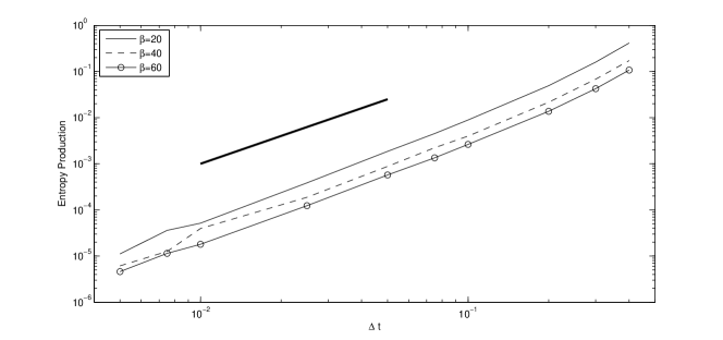
Figure 2. Entropy production rate as a function of time step $\Delta t$ for additive noise. The entropy production rate is of order $O(\Delta t^{2})$ for small $\Delta t$ while it decreases linearly as a function of inverse temperature $\beta$.

2.2. Entropy Production for the Multiplicative Noise Case: Euler-Marayuma scheme

In this section we consider the EM scheme for overdamped Langevin processes with multiplicative noise. For simplicity we restrict our discussion to the one dimensional case, but our results extend immediately to higher dimension if the the diffusion matrix $\sigma(x)$ is diagonal. We rewrite the GC action function given in Lemma 20,

$$W(n;\Delta t) \dot{=}-\frac{1}{2}\sum_{i=0}^{n-1}[V^{\prime}(x_{i+1})+V^{\prime}(x_{i})]\Delta x_{i}+\frac{1}{2}\sum_{i=0}^{n-1}[\Sigma^{-1}(x_{i+1})\Sigma^{\prime}(x_{i+1})+\Sigma^{-1}(x_{i})\Sigma^{\prime}(x_{i})]\Delta x_{i}$$ (41)

$$\quad+\frac{1}{2\Delta t}\sum_{i=0}^{n-1}\left[\Sigma^{-1}(x_{i+1})-\Sigma^{-1}(x_{i})\right]\Delta x_{i}^{2}$$

$$=:W_{1}(n;\Delta t)+W_{2}(n;\Delta t)+W_{3}(n;\Delta t)\,.$$

The first term $W_{1}(n;\Delta t)$ has been computed in the previous section and after an interesting and rather unexpected cancellation it was proved to be of order $O(\Delta t^{2})$. For the multiplicative case, a cancellation also occurs (see (45) and (46) below) but it does not fully eliminate the lower order term; in the end $W_{1}(n;\Delta t)$ contributes to the entropy production an $O(\Delta t)$ term. Additionally, $W_{2}(n;\Delta t)$ turns out to be the sum of gradient terms since $\Sigma^{-1}(x)\Sigma^{\prime}(x)=(\log\Sigma(x))^{\prime}$. Thus, assuming a suitable condition on $\Sigma(x)$, the same computation as for $W_{1}(n;\Delta t)$ applies and the entropy production rate stemming from $W_{2}(n;\Delta t)$ is also of order $O(\Delta t)$. However, $W_{3}(n;\Delta t)$ contributes to the entropy production a nonzero, positive term which is of order $O(1)$. The following theorem summarizes the behavior of entropy production rate for the explicit EM scheme for multiplicative noise. Let Assumption 1 hold and assume that the potential function $V$ has a bounded fifth-order derivative, while there exists $M>0$ such that $\Sigma(x)>M^{-1}$ for all $x$.
(a) If $c:=\frac{3}{4}\mathbb{E}_{\mu}[(\Sigma^{-1})(x)(\Sigma^{\prime})^{2}(x)]$, then, for sufficiently small $\Delta t$, there exists $C=C(V,\Sigma)>0$ independent of $\Delta t$ such that

$$|EP(\Delta t)-c|\leq C\Delta t$$ (42)

(b) Assuming that $\mathbb{E}_{\mu}[(\Sigma^{-1})(x)(\Sigma^{\prime})^{2}(x)]\neq 0$, then, for sufficiently small $\Delta t$, there exists a lower bound $c^{\prime}=c^{\prime}(V,\Sigma)>0$ independent of $\Delta t$ such that

$$c^{\prime}\leq EP(\Delta t)$$ (43)

Proof.

The assumption that $\Sigma(x)>M^{-1}\ \forall x$, which is the ellipticity condition in one space dimension, is necessary because it implies that $\Sigma^{-1}(x)$ as well its derivatives are bounded around 0. Additionally, as discussed earlier both $W_{1}(n;\Delta t)$ and $W_{2}(n;\Delta t)$ contribute to the entropy production by a $O(\Delta t)$ amount. Therefore we can concentrate on the term $W_{3}(n;\Delta t)$; after a Taylor series expansion we have,

$$W_{3}(n;\Delta t)=\frac{1}{2\Delta t}\sum_{i=0}^{n-1}\left[(\Sigma^{-1})^{\prime}(x_{i})\Delta x_{i}^{3}+\frac{1}{2}(\Sigma^{-1})^{\prime\prime}(x_{i})\Delta x_{i}^{4}+\frac{1}{2\Delta t}\sum_{i=0}^{n-1}\int_{0}^{1}(1-t)(\Sigma^{-1})^{\prime\prime\prime}(tx_{i+1}+(1-t)x_{i})dt\Delta x_{i}^{5}\right]$$

$$=\frac{1}{2\Delta t}\sum_{i=0}^{n-1}\sum_{k=0}^{3}\binom{3}{k}(\Sigma^{-1})^{\prime}(x_{i})(-\frac{1}{2}\Sigma(x_{i})V^{\prime}(x_{i})\Delta t+\frac{1}{2}\Sigma^{\prime}(x_{i})\Delta t)^{k}(\sigma(x_{i})\Delta W_{i})^{3-k}$$

$$+\frac{1}{4\Delta t}\sum_{i=0}^{n-1}\sum_{k=0}^{4}\binom{4}{k}(\Sigma^{-1})^{\prime\prime}(x_{i})(-\frac{1}{2}\Sigma(x_{i})V^{\prime}(x_{i})\Delta t+\frac{1}{2}\Sigma^{\prime}(x_{i})\Delta t)^{k}(\sigma(x_{i})\Delta W_{i})^{4-k}$$

$$+\frac{1}{2\Delta t}\sum_{i=0}^{n-1}\sum_{k=0}^{5}\binom{5}{k}\int_{0}^{1}(1-t)(\Sigma^{-1})^{\prime\prime\prime}(tx_{i+1}+(1-t)x_{i})dt(-\frac{1}{2}\Sigma(x_{i})V^{\prime}(x_{i})\Delta t+\frac{1}{2}\Sigma^{\prime}(x_{i})\Delta t)^{k}(\sigma(x_{i})\Delta W_{i})^{5-k}\,.$$

As in Theorem 2.1, applying the ergodic lemmas of the appendix, the entropy production rate stemming from $W_{3}(n;\Delta t)$ equals to

$$EP_{3}(\Delta t)=\lim_{t\rightarrow\infty}\frac{W_{3}(n;\Delta t)}{n\Delta t}$$ (44)

$$=\frac{1}{2\Delta t^{2}}\sum_{k=0}^{3}\binom{3}{k}\mathbb{E}_{\bar{\mu}}[(\Sigma^{-1})^{\prime}(x)(-\frac{1}{2}\Sigma(x)V^{\prime}(x)\Delta t+\frac{1}{2}\Sigma^{\prime}(x)\Delta t)^{k}\sigma(x)^{3-k}]\mathbb{E}_{\rho}[\Delta W^{3-k}]$$

$$+\frac{1}{4\Delta t^{2}}\sum_{k=0}^{4}\binom{4}{k}\mathbb{E}_{\bar{\mu}}[(\Sigma^{-1})^{\prime\prime}(x)(-\frac{1}{2}\Sigma(x)V^{\prime}(x)\Delta t+\frac{1}{2}\Sigma^{\prime}(x)\Delta t)^{k}\sigma(x)^{4-k}]\mathbb{E}_{\rho}[\Delta W^{4-k}]$$

$$+\frac{1}{2\Delta t^{2}}\sum_{k=0}^{5}\mathbb{E}_{\bar{\mu}\times\rho}[R(x,y)(-\frac{1}{2}\Sigma(x)V^{\prime}(x)\Delta t+\frac{1}{2}\Sigma^{\prime}(x)\Delta t)^{k}\sigma(x)^{5-k}]\mathbb{E}_{\rho}[\Delta W^{5-k}]$$

$$=\frac{1}{2\Delta t^{2}}\left[-\frac{3}{2}\mathbb{E}_{\bar{\mu}}[(\Sigma^{-1})^{\prime}(x)\Sigma^{2}(x)V^{\prime}(x)]\Delta t^{2}+\frac{3}{2}\mathbb{E}_{\bar{\mu}}[(\Sigma^{-1})^{\prime}(x)\Sigma^{\prime}(x)\Sigma(x)]\Delta t^{2}+O(\Delta t^{3})\right]$$

$$+\frac{1}{4\Delta t^{2}}\left[\mathbb{E}_{\bar{\mu}}[(\Sigma^{-1})^{\prime\prime}(x)\Sigma^{2}(x)]3\Delta t^{2}+O(\Delta t^{3})\right]+\frac{1}{2\Delta t^{2}}O(\Delta t^{3})$$

$$=\frac{3}{4}\left[-\mathbb{E}_{\bar{\mu}}[(\Sigma^{-1})^{\prime}(x)\Sigma^{2}(x)V^{\prime}(x)]+\frac{1}{2}\mathbb{E}_{\bar{\mu}}[(\Sigma^{-1})^{\prime}(x)(\Sigma^{2})^{\prime}(x)]+\mathbb{E}_{\bar{\mu}}[(\Sigma^{-1})^{\prime\prime}(x)\Sigma^{2}(x)]\right]+O(\Delta t)$$

On the other hand,

$$\mathbb{E}_{\mu}[(\Sigma^{-1})^{\prime}(x)\Sigma^{2}(x)V^{\prime}(x)]=\mathbb{E}_{\mu}[(\Sigma^{-1})^{\prime\prime}(x)\Sigma^{2}(x)]+\mathbb{E}_{\mu}[(\Sigma^{-1})^{\prime}(x)(\Sigma^{2})^{\prime}(x)]$$ (45)

Using (15) in Assumption 1 we obtain, as in the additive case, that

$$EP_{3}(\Delta t)-\frac{3}{4}\mathbb{E}_{\bar{\mu}}[(\Sigma^{-1})(x)(\Sigma^{\prime})^{2}(x)]=O(\Delta t)$$ (46)

which concludes the proof of (a). Part (b) is a direct consequence of (a). ∎

2.2.1. Example: Quadratic potential on $\mathbb{R}$

Let the quadratic potential $V(x)=\frac{x^{2}}{2}$ , and the diffusion term

$$\sigma_{\epsilon}(x)=\sqrt{\frac{1}{1+\epsilon x^{2}}}\,.$$ (47)

The choice of the diffusion term is justified by the fact that we can control its variation in terms of $x$, while sending $\epsilon$ to zero, the additive noise case is recovered. The invariant measure of this process is the Gaussian measure with zero mean and variance one. Moreover, all the assumptions of Theorem 43 are satisfied thus we expect a $O(1)$ behavior of the entropy production rate at least for small $\Delta t$. Indeed, Figure 3 shows the numerically-computed entropy production as a function of $\Delta t$, which clearly does not decrease to zero as $\Delta t$ tends to zero. Consequently, the explicit EM scheme for the multiplicative noise case totally destroys the reversibility property of the discrete-time approximation process independently of how small time-step is selected. Additionally, notice that as $\epsilon$ decreases, entropy production also decreases. This behavior is expected since $\sigma(x)\rightarrow\sigma=\text{constant}$ as $\epsilon\rightarrow 0$ and in combination with the quadratic potential $V$, $EP(\Delta t)\rightarrow 0$ as $\epsilon\rightarrow 0$ for any $\Delta t$ sufficiently small.

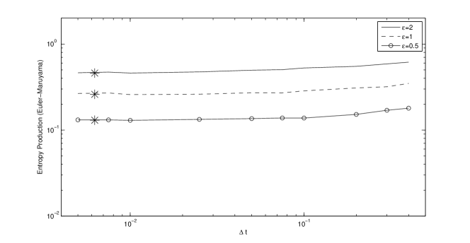
Figure 3. Entropy production rate as a function of time step $\Delta t$ for multiplicative noise and the explicit EM scheme. As Theorem 43 asserts, entropy production does not decrease as $\Delta t$ is decreased. This results in a permanent loss of reversibility which cannot be fixed by reducing the time step. Star symbols denote the theoretical value of the lower bound as it is given by the Theorem (i.e., $c^{\prime}\approx c=\frac{3}{4}\mathbb{E}_{\mu}[(\Sigma_{\epsilon})^{-1}(x)(\Sigma_{\epsilon}^{\prime})^{2}(x)]$). The agreement between the theoretical and the numerical values is excellent.

2.3. Entropy Production for the Multiplicative Noise Case: Milstein scheme

Since the EM scheme has entropy production rate which does not decrease as $\Delta t$ decreases, we turn our attention to the Milstein’s scheme which is the next higher-order scheme [10, 17]:

$$x_{i+1}=x_{i}-\frac{1}{2}\Sigma(x_{i})V^{\prime}(x_{i})\Delta t+\frac{1}{2}\Sigma^{\prime}(x_{i})\Delta t+\sigma(x_{i})\Delta W_{i}+\frac{1}{2}\sigma(x_{i})\sigma^{\prime}(x_{i})(\Delta W_{i}^{2}-\Delta t)\,,$$ (48)

which can be rewritten as

$$\Delta x_{i}=a(x_{i})\Delta t+\sigma(x_{i})\Delta W_{i}+\frac{1}{4}\Sigma^{\prime}(x_{i})\Delta W_{i}^{2}\,,$$ (49)

where $a(x_{i})=-\frac{1}{2}\Sigma(x_{i})V^{\prime}(x_{i})+\frac{1}{4}\Sigma^{\prime}(x_{i})$. Since $\Delta W_{i}$ is a zero-mean Gaussian random variable with variance $\Delta t$, the transition probability for Milstein’s scheme is

$$\Pi(x_{i},x_{i+1}) =\frac{1}{|\sqrt{2\pi\Delta tZ(x_{i},\Delta x_{i})}|}\left[\exp\left(-\frac{1}{2\Delta t}\left|\frac{-\sigma(x_{i})+\sqrt{Z(x_{i},\Delta x_{i})}}{\frac{1}{2}\Sigma^{\prime}(x_{i})}\right|^{2}\right)\right.$$ (50)

$$\left.+\exp\left(-\frac{1}{2\Delta t}\left|\frac{\sigma(x_{i})+\sqrt{Z(x_{i},\Delta x_{i})}}{\frac{1}{2}\Sigma^{\prime}(x_{i})}\right|^{2}\right)\right]$$

where

$$Z(x_{i},\Delta x_{i})=\Sigma(x_{i})+\Sigma^{\prime}(x_{i})\left(\Delta x_{i}-a(x_{i})\Delta t\right)\,.$$ (51)

Notice also that $Z(x_{i},\Delta x_{i})=(\sigma(x_{i})+\frac{1}{2}\Sigma^{\prime}(x_{i})\Delta W_{i})^{2}\geq 0$ which is positive almost surely. Moreover, the arguments of the exponentials in (50) are of different order in terms of $\Delta t$. Indeed, it is straightforward to show that for small time step, $\Delta t$, the argument of the first exponential in (50) is of order $O(1)$ while the argument of the second exponential is of order $O(\frac{1}{\Delta t})$. Thus, as $\Delta t$ tends to zero, the second exponential becomes exponentially small and the dominating term is the first exponential. Therefore, using the fact that $\log\left(e^{-a}+e^{-b/\Delta t}\right)=-a+O(e^{-b/\Delta t})$ for positive $a$ and $b$, the GC action functional for Milstein’s scheme reduces to

$$W(n;\Delta t) =-\frac{1}{2}\sum_{i=0}^{n-1}\log\frac{Z(x_{i},\Delta x_{i})}{Z(x_{i+1},-\Delta x_{i})}-\frac{2}{\Delta t}\sum_{i=0}^{n-1}\left[\left(\frac{-\sigma(x_{i})+\sqrt{Z(x_{i},\Delta x_{i})}}{\frac{1}{2}\Sigma^{\prime}(x_{i})}\right)^{2}-\left(\frac{-\sigma(x_{i+1})+\sqrt{Z(x_{i+1},-\Delta x_{i})}}{\frac{1}{2}\Sigma^{\prime}(x_{i+1})}\right)^{2}\right]$$ (52)

$$=W_{1}(n;\Delta t)+W_{2}(n;\Delta t)$$

where $Z(x_{i+1},-\Delta x_{i})=\Sigma(x_{i+1})+\Sigma^{\prime}(x_{i+1})\left(-\Delta x_{i}-a(x_{i+1})\Delta t\right)$. The following theorem demonstrates that the entropy production of the Milstein Scheme is at least linear in $\Delta t$:

Under the assumptions of Theorem 43 and for sufficiently small $\Delta t$, there exists $C=C(V,\Sigma)>0$ independent of $\Delta t$ such that

$$EP(\Delta t)\leq C\Delta t$$ (53)

Proof.

In order to compute the detailed asymptotics for $W_{1}(n;\Delta t)$ and $W_{2}(n;\Delta t)$ we write the partition function $Z(x_{i},\Delta x_{i})$ as

$$Z(x_{i},\Delta x_{i}) =\Sigma(x_{i})+\Sigma^{\prime}(x_{i})\left(\Delta x_{i}-a(x_{i})\Delta t\right)$$ (54)

$$=\Sigma(x_{i+1})-\left(\frac{1}{2}\Sigma^{\prime\prime}(x_{i})\Delta x_{i}^{2}+\frac{1}{6}\Sigma^{\prime\prime\prime}(x_{i})\Delta x_{i}^{3}+\Sigma^{\prime}(x_{i})a(x_{i})\Delta t\right)+O(\Delta x_{i}^{4})\ .$$

Similarly we have

$$Z(x_{i+1},-\Delta x_{i}) =\Sigma(x_{i+1})+\Sigma^{\prime}(x_{i+1})\left(-\Delta x_{i}-a(x_{i+1})\Delta t\right)$$ (55)

$$=\Sigma(x_{i})-\left(\frac{1}{2}\Sigma^{\prime\prime}(x_{i+1})\Delta x_{i}^{2}-\frac{1}{6}\Sigma^{\prime\prime\prime}(x_{i+1})\Delta x_{i}^{3}+\Sigma^{\prime}(x_{i+1})a(x_{i+1})\Delta t\right)+O(\Delta x_{i}^{4})\ ,$$

and thus

$$Z(x_{i+1},-\Delta x_{i})-Z(x_{i-1},\Delta x_{i-1})=-\frac{1}{2}(\Sigma^{\prime\prime}(x_{i+1})\Delta x_{i}^{2}-\Sigma^{\prime\prime}(x_{i-1})\Delta x_{i-1}^{2})$$ (56)

$$+\frac{1}{6}(\Sigma^{\prime\prime\prime}(x_{i+1})\Delta x_{i}^{3}+\Sigma^{\prime\prime\prime}(x_{i-1})\Delta x_{i-1}^{3})-(\Sigma^{\prime}(x_{i+1})a(x_{i+1})-\Sigma^{\prime}(x_{i-1})a(x_{i-1}))\Delta t$$

is obtained. Moreover, in what follows and by slight abuse of $O(\cdot)$ notation, we repeatedly use the relation

$$\left[f(x_{i})g(x_{i\pm 1})-f(x_{i\pm 1})g(x_{i})\right]\Delta x_{i}^{k}=O(\Delta x_{i}^{k+1})$$ (57)

which holds for any $i,k=0,1,...$ and any smooth functions $f$ and $g$ and it is easily derived by suitable Taylor expansions of the functions. We obtain for $W_{1}(n;\Delta t)$

$$W_{1}(n;\Delta t) =\frac{1}{2}\sum_{i=0}^{n-1}\log\frac{Z(x_{i+1},-\Delta x_{i})}{Z(x_{i},\Delta x_{i})}$$ (58)

$$\dot{=}\frac{1}{2}\sum_{i=0}^{n-1}\log\frac{Z(x_{i+1},-\Delta x_{i})}{Z(x_{i-1},\Delta x_{i-1})}$$

$$=\frac{1}{2}\sum_{i=0}^{n-1}\log\left(1-\frac{\frac{1}{2}(\Sigma^{\prime\prime}(x_{i+1})\Delta x_{i}^{2}-\Sigma^{\prime\prime}(x_{i-1})\Delta x_{i-1}^{2})+(\Sigma^{\prime}(x_{i+1})a(x_{i+1})-\Sigma^{\prime}(x_{i-1})a(x_{i-1}))\Delta t+O(\Delta x_{i}^{3})}{Z(x_{i-1},\Delta x_{i-1})}\right)$$

$$=\frac{1}{2}\sum_{i=0}^{n-1}\sum_{k=1}^{\infty}\left(\frac{\frac{1}{2}(\Sigma^{\prime\prime}(x_{i+1})\Delta x_{i}^{2}-\Sigma^{\prime\prime}(x_{i-1})\Delta x_{i-1}^{2})+O(\Delta t\Delta x_{i}+\Delta x_{i}^{3})}{Z(x_{i-1},\Delta x_{i-1})}\right)^{k}$$

$$=\frac{1}{4}\sum_{i=0}^{n-1}\left[\frac{\Sigma^{\prime\prime}(x_{i+1})\Delta x_{i}^{2}-\Sigma^{\prime\prime}(x_{i-1})\Delta x_{i-1}^{2}}{\Sigma(x_{i})+O(\Delta t+\Delta x_{i}^{2})}+O(\Delta t\Delta x_{i}+\Delta x_{i}^{3})\right]$$

$$=\frac{1}{4}\sum_{i=0}^{n-1}\left[\frac{\Sigma^{\prime\prime}(x_{i+1})\Delta x_{i}^{2}-\Sigma^{\prime\prime}(x_{i-1})\Delta x_{i-1}^{2}}{\Sigma(x_{i})}\sum_{k=0}^{\infty}\left(O(\Delta t+\Delta x_{i}^{2})\right)^{k}+O(\Delta t\Delta x_{i}+\Delta x_{i}^{3})\right]$$

$$=\frac{1}{4}\sum_{i=0}^{n-1}\left[\frac{\Sigma^{\prime\prime}(x_{i+1})\Delta x_{i}^{2}-\Sigma^{\prime\prime}(x_{i-1})\Delta x_{i-1}^{2}}{\Sigma(x_{i})}+O(\Delta t\Delta x_{i}+\Delta x_{i}^{3})\right]$$

$$\dot{=}\frac{1}{4}\sum_{i=0}^{n-1}\left[\left(\frac{1}{\Sigma(x_{i})}-\frac{1}{\Sigma(x_{i+1})}\right)\Sigma^{\prime\prime}(x_{i})\Delta x_{i}^{2}+O(\Delta t\Delta x_{i}+\Delta x_{i}^{3})\right]$$

$$=\sum_{i=0}^{n-1}O(\Delta x_{i}^{3})+\Delta t\sum_{i=0}^{n-1}O(\Delta x_{i})$$

The second term of the GC action functional is rewritten as

$$W_{2}(n;\Delta t) =\frac{2}{\Delta t}\sum_{i=0}^{n-1}\left[\left(\frac{\sigma(x_{i+1})-\sqrt{Z(x_{i+1},-\Delta x_{i})}}{\frac{1}{2}\Sigma^{\prime}(x_{i+1})}\right)^{2}-\left(\frac{\sigma(x_{i})-\sqrt{Z(x_{i},\Delta x_{i})}}{\frac{1}{2}\Sigma^{\prime}(x_{i})}\right)^{2}\right]$$ (59)

$$=\frac{2}{\Delta t}\sum_{i=0}^{n-1}\left[\left(\frac{\sigma(x_{i+1})-\sigma(x_{i})\Big{(}1-\frac{1}{2\Sigma(x_{i})}\big{(}\frac{1}{2}\Sigma^{\prime\prime}(x_{i+1})\Delta x_{i}^{2}-\frac{1}{6}\Sigma^{\prime\prime\prime}(x_{i+1})\Delta x_{i}^{3}+\Sigma^{\prime}(x_{i+1})a(x_{i+1})\Delta t+O(\Delta x_{i}^{4})\big{)}\Big{)}}{\frac{1}{2}\Sigma^{\prime}(x_{i+1})}\right)^{2}\right.$$

$$\left.-\left(\frac{\sigma(x_{i})-\sigma(x_{i+1})\Big{(}1-\frac{1}{2\Sigma(x_{i+1})}\big{(}\frac{1}{2}\Sigma^{\prime\prime}(x_{i})\Delta x_{i}^{2}+\frac{1}{6}\Sigma^{\prime\prime\prime}(x_{i})\Delta x_{i}^{3}+\Sigma^{\prime}(x_{i})a(x_{i})\Delta t+O(\Delta x_{i}^{4})\big{)}\Big{)}}{\frac{1}{2}\Sigma^{\prime}(x_{i})}\right)^{2}\right]$$

$$=\frac{2}{\Delta t}\sum_{i=0}^{n-1}\left[\left(2\frac{\sigma(x_{i+1})-\sigma(x_{i})}{\Sigma^{\prime}(x_{i+1})}+\frac{1}{2}\frac{\Sigma^{\prime\prime}(x_{i+1})\Delta x_{i}^{2}}{\sigma(x_{i})\Sigma^{\prime}(x_{i+1})}-\frac{1}{6}\frac{\Sigma^{\prime\prime\prime}(x_{i+1})\Delta x_{i}^{3}}{\sigma(x_{i})\Sigma^{\prime}(x_{i+1})}+\frac{1}{2}\frac{\Sigma^{\prime}(x_{i+1})a(x_{i+1})\Delta t}{\sigma(x_{i})\Sigma^{\prime}(x_{i+1})}+O(\Delta x_{i}^{4})\right)^{2}\right.$$

$$\left.-\left(2\frac{\sigma(x_{i})-\sigma(x_{i+1})}{\Sigma^{\prime}(x_{i})}+\frac{1}{2}\frac{\Sigma^{\prime\prime}(x_{i})\Delta x_{i}^{2}}{\sigma(x_{i+1})\Sigma^{\prime}(x_{i})}+\frac{1}{6}\frac{\Sigma^{\prime\prime\prime}(x_{i})\Delta x_{i}^{3}}{\sigma(x_{i+1})\Sigma^{\prime}(x_{i})}+\frac{1}{2}\frac{\Sigma^{\prime}(x_{i})a(x_{i})\Delta t}{\sigma(x_{i+1})\Sigma^{\prime}(x_{i})}+O(\Delta x_{i}^{4})\right)^{2}\right]$$

where a Taylor series expansion to the square root function was applied. Expanding the squares and keeping only the terms that have order in terms of $\Delta x_{i}$ less than 5 we obtain that

$$W_{2}(n;\Delta t) =\frac{2}{\Delta t}\sum_{i=0}^{n-1}\left[4\left(\frac{(\sigma(x_{i+1})-\sigma(x_{i}))^{2}}{\Sigma^{\prime}(x_{i+1})^{2}}-\frac{(\sigma(x_{i+1})-\sigma(x_{i}))^{2}}{\Sigma^{\prime}(x_{i})^{2}}\right)\right.$$ (60)

$$+2\left(\frac{\Sigma^{\prime\prime}(x_{i+1})(\sigma(x_{i+1})-\sigma(x_{i}))}{\sigma(x_{i})\Sigma^{\prime}(x_{i+1})^{2}}+\frac{\Sigma^{\prime\prime}(x_{i})(\sigma(x_{i+1})-\sigma(x_{i}))}{\sigma(x_{i+1})\Sigma^{\prime}(x_{i})^{2}}\right)\Delta x_{i}^{2}$$

$$-\frac{2}{3}\left(\frac{\Sigma^{\prime\prime\prime}(x_{i+1})(\sigma(x_{i+1})-\sigma(x_{i}))}{\sigma(x_{i})\Sigma^{\prime}(x_{i+1})^{2}}-\frac{\Sigma^{\prime\prime\prime}(x_{i})(\sigma(x_{i+1})-\sigma(x_{i}))}{\sigma(x_{i+1})\Sigma^{\prime}(x_{i})^{2}}\right)\Delta x_{i}^{3}$$

$$+4\left(\frac{a(x_{i+1})(\sigma(x_{i+1})-\sigma(x_{i}))}{\sigma(x_{i})\Sigma^{\prime}(x_{i+1})}+\frac{a(x_{i})(\sigma(x_{i+1})-\sigma(x_{i}))}{\sigma(x_{i+1})\Sigma^{\prime}(x_{i})}\right)\Delta t$$

$$\left.+\left(\frac{\Sigma^{\prime\prime}(x_{i+1})a(x_{i+1})}{\Sigma(x_{i})\Sigma^{\prime}(x_{i+1})}-\frac{\Sigma^{\prime\prime}(x_{i})a(x_{i})}{\Sigma(x_{i+1})\Sigma^{\prime}(x_{i})}\right)\Delta t\Delta x_{i}^{2}+O(\Delta x_{i}^{5})+O(\Delta t\Delta x_{i}^{3})\right]$$

$$=\frac{2}{\Delta t}\sum_{i=0}^{n-1}\left[\frac{\sigma^{\prime}(x_{i+1})^{2}\Delta x_{i}^{2}-\sigma^{\prime}(x_{i+1})\sigma^{\prime\prime}(x_{i+1})\Delta x_{i}^{3}+\left(\frac{1}{3}\sigma^{\prime}(x_{i+1})\sigma^{\prime\prime\prime}(x_{i+1})+\frac{1}{4}\sigma^{\prime\prime}(x_{i+1})^{2}\right)\Delta x_{i}^{4}}{\sigma(x_{i+1})^{2}\sigma^{\prime}(x_{i+1})^{2}}\right.$$

$$-\frac{\sigma^{\prime}(x_{i})^{2}\Delta x_{i}^{2}+\sigma^{\prime}(x_{i})\sigma^{\prime\prime}(x_{i})\Delta x_{i}^{3}+\left(\frac{1}{3}\sigma^{\prime}(x_{i})\sigma^{\prime\prime\prime}(x_{i})+\frac{1}{4}\sigma^{\prime\prime}(x_{i})^{2}\right)\Delta x_{i}^{4}}{\sigma(x_{i})^{2}\sigma^{\prime}(x_{i})^{2}}$$

$$+2\frac{\sigma(x_{i+1})(\sigma^{\prime}(x_{i+1})\Delta x_{i}-\frac{1}{2}\sigma^{\prime\prime}(x_{i+1})\Delta x_{i}^{2})\Sigma^{\prime\prime}(x_{i+1})\Sigma^{\prime}(x_{i})^{2}+\sigma(x_{i})(\sigma^{\prime}(x_{i})\Delta x_{i}+\frac{1}{2}\sigma^{\prime\prime}(x_{i})\Delta x_{i}^{2})\Sigma^{\prime\prime}(x_{i})\Sigma^{\prime}(x_{i+1})^{2}}{\sigma(x_{i})\sigma(x_{i+1})\Sigma^{\prime}(x_{i})^{2}\Sigma^{\prime}(x_{i+1})^{2}}\Delta x_{i}^{2}$$

$$\left.+2\left(\frac{a(x_{i+1})(\sigma^{\prime}(x_{i+1})\Delta x_{i}-\frac{1}{2}\sigma^{\prime\prime}(x_{i+1})\Delta x_{i}^{2})}{\sigma(x_{i+1})\sigma^{\prime}(x_{i+1})\sigma(x_{i})}+\frac{a(x_{i})(\sigma^{\prime}(x_{i})\Delta x_{i}+\frac{1}{2}\sigma^{\prime\prime}(x_{i})\Delta x_{i}^{2})}{\sigma(x_{i})\sigma^{\prime}(x_{i})\sigma(x_{i+1})}\right)\Delta t+O(\Delta x_{i}^{5})+O(\Delta t\Delta x_{i}^{3})\right]$$

$$=\frac{2}{\Delta t}\sum_{i=0}^{n-1}\left[\left(\frac{1}{\sigma(x_{i+1})^{2}}-\frac{1}{\sigma(x_{i})^{2}}\right)\Delta x_{i}^{2}-\left(\frac{\sigma^{\prime\prime}(x_{i+1})}{\sigma(x_{i+1})^{2}\sigma^{\prime}(x_{i+1})}+\frac{\sigma^{\prime\prime}(x_{i})}{\sigma(x_{i})^{2}\sigma^{\prime}(x_{i})}\right)\Delta x_{i}^{3}\right.$$

$$\left.+\frac{\Sigma^{\prime\prime}(x_{i+1})\Sigma^{\prime}(x_{i})+\Sigma^{\prime\prime}(x_{i})\Sigma^{\prime}(x_{i+1})}{\sigma(x_{i})\sigma(x_{i+1})\Sigma^{\prime}(x_{i})\Sigma^{\prime}(x_{i+1})}\Delta x_{i}^{3}+2\frac{a(x_{i+1})+a(x_{i})}{\sigma(x_{i})\sigma(x_{i+1})}\Delta x_{i}\Delta t+O(\Delta x_{i}^{5})+O(\Delta t\Delta x_{i}^{3})\right]$$

$$=\frac{2}{\Delta t}\sum_{i=0}^{n-1}\left[-\left(\frac{\sigma^{\prime}(x_{i+1})}{\sigma(x_{i+1})^{3}}+\frac{\sigma^{\prime}(x_{i})}{\sigma(x_{i})^{3}}+\frac{\sigma^{\prime\prime}(x_{i+1})}{\sigma(x_{i+1})^{2}\sigma^{\prime}(x_{i+1})}+\frac{\sigma^{\prime\prime}(x_{i})}{\sigma(x_{i})^{2}\sigma^{\prime}(x_{i})}\right)\Delta x_{i}^{3}\right.$$

$$\left.+\left(\frac{\sigma^{\prime}(x_{i+1})}{\sigma(x_{i+1})^{2}\sigma(x_{i})}+\frac{\sigma^{\prime\prime}(x_{i+1})}{\sigma(x_{i+1})\sigma^{\prime}(x_{i+1})\sigma(x_{i})}+\frac{\sigma^{\prime}(x_{i})}{\sigma(x_{i})^{2}\sigma(x_{i+1})}+\frac{\sigma^{\prime\prime}(x_{i})}{\sigma(x_{i})\sigma^{\prime}(x_{i})\sigma(x_{i+1})}\right)\Delta x_{i}^{3}+O(\Delta x_{i}^{5})\right]$$

$$+4\sum_{i=0}^{n-1}\left[\left(\frac{a(x_{i+1})}{\Sigma(x_{i+1})}+\frac{a(x_{i})}{\Sigma(x_{i})}\right)\Delta x_{i}+O(\Delta x_{i}^{3})\right]$$

After few more Taylor expansions in the first sum, the terms of order $\Delta x_{i}^{3}$ are cancelled out while the forth order terms consists of differences of the form (57) thus they become fifth order. Moreover, the second sum can be handled exactly as the terms $W_{1}$ and $W_{2}$ in EM scheme using (84) and the leading term is of order $O(\Delta x_{i}^{3})$. Overall, we rigorously computed that

$$W_{2}(n;\Delta t)\dot{=}\frac{1}{\Delta t}\sum_{i=0}^{n-1}O(\Delta x_{i}^{5})+\sum_{i=0}^{n-1}O(\Delta x_{i}^{3})\ .$$ (61)

Therefore, the entropy production for Milstein’s scheme in the one dimensional overdamped Langevin case with multiplicative noise is at least of order

$$EP(\Delta t) =\lim_{t\rightarrow\infty}\frac{1}{n\Delta t}(W_{1}(n;\Delta t)+W_{2}(n;\Delta t))$$ (62)

$$=\lim_{n\rightarrow\infty}\frac{1}{n}\sum_{i=0}^{n-1}O(\Delta x_{i})+\frac{1}{\Delta t}\lim_{n\rightarrow\infty}\frac{1}{n}\sum_{i=0}^{n-1}O(\Delta x_{i}^{3})+\frac{1}{\Delta t^{2}}\lim_{n\rightarrow\infty}\frac{1}{n}\sum_{i=0}^{n-1}O(\Delta x_{i}^{5})$$

$$=O(\Delta t)+\frac{1}{\Delta t}O(\Delta t^{2})+\frac{1}{\Delta t^{2}}O(\Delta t^{3})$$

$$=O(\Delta t)\,.$$

Here we used the fact that $\lim_{n\rightarrow\infty}\frac{1}{n}\sum_{i=0}^{n-1}f(x_{i})\Delta x_{i}^{k}=O(\Delta t^{\lceil\frac{k}{2}\rceil})$, where $\lceil\cdot\rceil$ denotes the ceiling function; this last relation is easily verified by substituting $\Delta x_{i}$ by (LABEL:multi:sde:explMilstein) and then applying the ergodic average lemmas in Appendix A. ∎

2.3.1. Quadratic potential on $\mathbb{R}$

We compute numerically the entropy production as the time-average of the GC action functional. Figure 4 shows the numerically computed entropy production for the same example shown in Figure 3. Evidently, entropy production rate decreases at least linearly as time step $\Delta t$ is decreasing as Theorem 53 asserts.

We note that the rigorous asymptotics for the entropy production quickly become quite involved as the Milstein scheme analysis demonstrates. However, the GC functional is easily accessible numerically and this allows to assess the reversibility of each scheme computationally, as demonstrated in Figure 3 and Figure 4.

Figure 4. Entropy production rate as a function of time step $\Delta t$ for the explicit Milstein’s scheme. The decrease of the entropy production rate for this numerical scheme is linear.

3. Entropy Production for Langevin Processes

Let us consider another important class of reversible processes, namely the processes driven by the Langevin equation

$$dq_{t}=M^{-1}p_{t}dt$$ (63)

$$dp_{t}=-\nabla V(q_{t})dt-\gamma M^{-1}p_{t}dt+\sigma dB_{t}$$

where $q_{t}\in\mathbb{R}^{dN}$ is the position vector of the $N$ particles, $p_{t}\in\mathbb{R}^{dN}$ is the momentum vector of the particles, $M$ is the mass matrix, $V$ is the potential energy, $\gamma$ is the friction factor (matrix), $\sigma$ is the diffusion factor (matrix) and $B_{t}$ is a $dN$-dimensional Brownian motion. Even though the Langevin system is degenerate since the noise applies only to the momenta, the process is hypoelliptic and is ergodic under mild conditions on $V$. The fluctuation-dissipation theorem asserts that friction and diffusion terms are related with the inverse temperature $\beta\in\mathbb{R}$ of the system by

$$(\sigma\sigma^{T})=2\beta^{-1}\gamma\,.$$ (64)

The Langevin system is reversible (modulo momenta flip, see (67)) with invariant measure

$$\mu(dq,dp)=\frac{1}{Z}\exp\left(-\beta H(q,p)\right)dqdp.$$ (65)

where $H(q,p)$ is the Hamiltonian of the system given by

$$H(q,p)=V(q)+\frac{1}{2}p^{T}M^{-1}p\,.$$ (66)

Indeed if $\mathcal{L}$ denotes the generator of (63), it is straightforward to verify the following modified DB condition

$$<\mathcal{L}f(q,p),g(q,p)>_{L^{2}(\mu)}=<f(q,-p),\mathcal{L}g(q,-p)>_{L^{2}(\mu)}$$ (67)

for any test functions $f$ and $g$ which are bounded, twice differentiable with bounded derivatives. This shows that the Langevin process is reversible modulo flipping the momenta of all particles.

The BBK integrator [4, 12] which utilizes a Strang splitting is applied for the discretization of (63). It is written as

$$p_{i+\frac{1}{2}} =p_{i}-\nabla V(q_{i})\frac{\Delta t}{2}-\gamma M^{-1}p_{i}\frac{\Delta t}{2}+\sigma\Delta W_{i}$$ (68)

$$q_{i+1} =q_{i}+M^{-1}p_{i+\frac{1}{2}}\Delta t$$

$$p_{i+1} =p_{i+\frac{1}{2}}-\nabla V(q_{i+1})\frac{\Delta t}{2}-\gamma M^{-1}p_{i+1}\frac{\Delta t}{2}+\sigma\Delta W_{i+\frac{1}{2}}$$

with $\Delta W_{i},\Delta W_{i+\frac{1}{2}}\sim N(0,\frac{\Delta t}{2}I_{dN})$. Its stability and convergence properties were studied in [4, 12] while its ergodic properties can be found in [26, 15, 14]. An important property of this numerical scheme which simplifies the computation of the transition probabilities is that the transition probabilities are non-degenerate. We rewrite the BBK integrator as

$$q_{i+1}=q_{i}+M^{-1}[p_{i}-\nabla V(q_{i})\frac{\Delta t}{2}-\gamma M^{-1}p_{i}\frac{\Delta t}{2}]\Delta t+M^{-1}\sigma\Delta t\Delta W_{i}\\$$ (69a)

$$p_{i+1}=(I+\gamma M^{-1}\frac{\Delta t}{2})^{-1}[\frac{1}{\Delta t}M(q_{i+1}-q_{i})-\nabla V(q_{i+1})\frac{\Delta t}{2}]+(I+\gamma M^{-1}\frac{\Delta t}{2})^{-1}\sigma\Delta W_{i+\frac{1}{2}}$$ (69b)

and thus the transition probabilities of the discrete-time approximation process are given by the product

$$\Pi(q_{i},p_{i},q_{i+1},p_{i+1})=P(q_{i+1}|q_{i},p_{i})P(p_{i+1}|q_{i+1},q_{i},p_{i})$$ (70)

where $P(q_{i+1}|q_{i},p_{i})$ is the propagator of the positions given by

$$P(q_{i+1}|q_{i},p_{i}) =\frac{1}{Z_{0}}\exp\{-\frac{1}{\Delta t^{3}}(\Delta q_{i}+M^{-1}(p_{i}-\nabla V(q_{i})\frac{\Delta t}{2}+\gamma M^{-1}p_{i}\frac{\Delta t}{2})\Delta t)^{T}$$ (71)

$$(\sigma M^{-T}M^{-1}\sigma^{T})^{-1}(\Delta q_{i}+M^{-1}(p_{i}-\nabla V(q_{i})\frac{\Delta t}{2}+\gamma M^{-1}p_{i}\frac{\Delta t}{2})\Delta t)\}$$

where $\Delta q_{i}=q_{i+1}-q_{i}$ while $P(p_{i+1}|q_{i+1},q_{i},p_{i})$ is the propagator of the momenta given by

$$P(p_{i+1}|q_{i+1},q_{i},p_{i})=\frac{1}{Z_{1}}\exp\{-\frac{1}{\Delta t}(p_{i+1}-(I+\gamma)M^{-1}\frac{\Delta t}{2})^{-1}(\frac{1}{\Delta t}M\Delta q_{i}-\nabla V(q_{i+1})\frac{\Delta t}{2}))^{T}$$ (72)

$$(\sigma^{T}(I+\gamma M)^{-T}(I+\gamma M^{-1})\sigma)^{-1}(p_{i+1}-(I+\gamma)M^{-1}\frac{\Delta t}{2})^{-1}(\frac{1}{\Delta t}M\Delta q_{i}-\nabla V(q_{i+1})\frac{\Delta t}{2}))\}$$

Finally, since the Langevin process is reversible modulo flip of the momenta, the GC action functional takes the form

$$W(n;\Delta t)=\sum_{i=0}^{n-1}\log\frac{\Pi(q_{i},p_{i},q_{i+1},p_{i+1})}{\Pi(q_{i+1},-p_{i+1},q_{i},-p_{i})}.$$ (73)

3.1. Langevin Process with Additive Noise

In the following we assume for simplicity that particles have equal masses (i.e. $M=mI$) and that $\sigma=\sigma I$, $\gamma=\gamma I$. In the next lemma we compute the GC action functional.

The GC action functional of the BBK integrator equals to

$$W(n;\Delta t)\dot{=}\frac{\beta}{\Delta t}\sum_{i=0}^{n-1}\left[\Delta p_{i}^{T}\Delta q_{i}-\frac{\Delta t^{2}}{2m}(\nabla V(q_{i})^{T}p_{i}+\nabla V(q_{i+1})^{T}p_{i+1})\right]$$ (74)

Proof.

Firstly, (LABEL:trans:prob:position) and (LABEL:trans:prob:momenta) are rewritten as

$$P(q_{i+1}|q_{i},p_{i})=\frac{1}{Z_{0}}\exp\left\{-\frac{m^{2}}{\sigma^{2}\Delta t^{3}}|\Delta q_{i}+(p_{i}-\frac{1}{m}\nabla V(q_{i})\frac{\Delta t}{2}+\frac{\gamma}{m}p_{i}\frac{\Delta t}{2})\Delta t|^{2}\right\}$$ (75)

and

$$P(p_{i+1}|q_{i+1},q_{i},p_{i})=\frac{1}{Z_{1}}\exp\left\{-\frac{1}{\sigma^{2}\Delta t}|(1+\frac{\gamma\Delta t}{2m})p_{i+1}-(\frac{m}{\Delta t}\Delta q_{i}-\frac{\Delta t}{2}\nabla V(q_{i+1}))|^{2}\right\}$$ (76)

respectively. Then, as in the overdamped Langevin case, the computation of the GC action functional is straightforward,

$$W(n;\Delta t) =-\frac{m^{2}}{\sigma^{2}\Delta t^{3}}\sum_{i=0}^{n-1}\left[\left|\Delta q_{i}+\frac{\Delta t^{2}}{2m}\nabla V(q_{i})-\frac{\Delta t}{m}(1-\frac{\gamma\Delta t}{2m})p_{i}\right|^{2}-\left|-\Delta q_{i}+\frac{\Delta t^{2}}{2m}\nabla V(q_{i+1})+\frac{\Delta t}{m}(1-\frac{\gamma\Delta t}{2m})p_{i+1}\right|^{2}\right]$$

$$-\frac{1}{\sigma^{2}\Delta t}\sum_{i=0}^{n-1}\left[\left|(1+\frac{\gamma\Delta t}{2m})p_{i+1}-\frac{m}{\Delta t}\Delta q_{i}+\frac{\Delta t}{2}\nabla V(q_{i+1})\right|^{2}-\left|-(1+\frac{\gamma\Delta t}{2m})p_{i}+\frac{m}{\Delta t}\Delta q_{i}+\frac{\Delta t}{2}\nabla V(q_{i})\right|^{2}\right]$$

$$=-\frac{m^{2}}{\sigma^{2}\Delta t^{3}}\sum_{i=0}^{n-1}\left[|\Delta q_{i}|^{2}+|\frac{\Delta t^{2}}{2m}\nabla V(q_{i})|^{2}+|\frac{\Delta t}{m}(1-\frac{\gamma\Delta t}{2m})p_{i}|^{2}+\frac{\Delta t^{2}}{m}\Delta q_{i}^{T}\nabla V(q_{i})\right.$$

$$-\frac{2\Delta t}{m}(1-\frac{\gamma\Delta t}{2m})\Delta q_{i}^{T}p_{i}-\frac{\Delta t^{3}}{m^{2}}(1-\frac{\gamma\Delta t}{2m})\nabla V(q_{i})^{T}p_{i}$$

$$-|\Delta q_{i}|^{2}-|\frac{\Delta t^{2}}{2m}\nabla V(q_{i+1})|^{2}-|\frac{\Delta t}{m}(1-\frac{\gamma\Delta t}{2m})p_{i+1}|^{2}+\frac{\Delta t^{2}}{m}\Delta q_{i}^{T}\nabla V(q_{i+1})$$

$$\left.+\frac{2\Delta t}{m}(1-\frac{\gamma\Delta t}{2m})\Delta q_{i}^{T}p_{i+1}-\frac{\Delta t^{3}}{m^{2}}(1-\frac{\gamma\Delta t}{2m})\nabla V(q_{i+1})^{T}p_{i+1}\right]$$

$$-\frac{1}{\sigma^{2}\Delta t}\sum_{i=0}^{n-1}\left[|(1+\frac{\gamma\Delta t}{2m})p_{i+1}|^{2}+|\frac{m}{\Delta t}\Delta q_{i}|^{2}+|\frac{\Delta t}{2}\nabla V(q_{i+1})|^{2}-(1+\frac{\gamma\Delta t}{2m})\frac{2m}{\Delta t}p_{i+1}^{T}\Delta q_{i}\right.$$

$$+(1+\frac{\gamma\Delta t}{2m})\Delta tp_{i+1}^{T}\nabla V(q_{i+1})-m\Delta q_{i}^{T}\nabla V(q_{i+1})$$

$$-|(1+\frac{\gamma\Delta t}{2m})p_{i}|^{2}-|\frac{m}{\Delta t}\Delta q_{i}|^{2}-|\frac{\Delta t}{2}\nabla V(q_{i})|^{2}+(1+\frac{\gamma\Delta t}{2m})\frac{2m}{\Delta t}p_{i}^{T}\Delta q_{i}$$

$$+\left.(1+\frac{\gamma\Delta t}{2m})\Delta tp_{i}^{T}\nabla V(q_{i})-m\Delta q_{i}^{T}\nabla V(q_{i})\right]\,.$$

Thus we have,

$$W(n;\Delta t) \dot{=}-\frac{m^{2}}{\sigma^{2}\Delta t^{3}}\sum_{i=0}^{n-1}\left[\frac{\Delta t^{2}}{m}\Delta q_{i}^{T}(\nabla V(q_{i})+\nabla V(q_{i+1}))+\frac{2\Delta t}{m}(1-\frac{\gamma\Delta t}{2m})\Delta q_{i}^{T}\Delta p_{i}\right.$$

$$\left.-\frac{\Delta t^{3}}{m^{2}}(1-\frac{\gamma\Delta t}{2m})(\nabla V(q_{i+1})^{T}p_{i+1}+\nabla V(q_{i})^{T}p_{i})\right]$$

$$-\frac{1}{\sigma^{2}\Delta t}\sum_{i=0}^{n-1}\left[-(1+\frac{\gamma\Delta t}{2m})\frac{2m}{\Delta t}\Delta p_{i}^{T}\Delta q_{i}-m\Delta q_{i}^{T}(\nabla V(q_{i})+\nabla V(q_{i+1}))\right.$$

$$\left.+(1+\frac{\gamma\Delta t}{2m})\Delta t(p_{i}^{T}\nabla V(q_{i})+p_{i+1}^{T}\nabla V(q_{i+1}))\right]$$

$$=\frac{2m}{\sigma^{2}\Delta t^{2}}\sum_{i=0}^{n-1}\left[-(1-\frac{\gamma\Delta t}{2m})\Delta q_{i}^{T}\Delta p_{i}+(1+\frac{\gamma\Delta t}{2m})\Delta q_{i}^{T}\Delta p_{i}\right.$$

$$\left.+\frac{\Delta t^{2}}{2m}(1-\frac{\gamma\Delta t}{2m})(\nabla V(q_{i+1})^{T}p_{i+1}+\nabla V(q_{i})^{T}p_{i})-\frac{\Delta t^{2}}{2m}(1+\frac{\gamma\Delta t}{2m})(\nabla V(q_{i+1})^{T}p_{i+1}+\nabla V(q_{i})^{T}p_{i})\right]$$

$$=\frac{2\gamma}{\sigma^{2}\Delta t}\sum_{i=0}^{n-1}\left[\Delta p_{i}^{T}\Delta q_{i}-\frac{\Delta t^{2}}{2m}(\nabla V(q_{i+1})^{T}p_{i+1}+\nabla V(q_{i})^{T}p_{i})\right]$$

which is equal with (74). ∎

Proceeding as in Remark 2 we can compare the GC action functional of the BBK integrator to the GC functional for the additive Langevin process with constant temperature, which is given, [13], by

$$W_{cont}(t)=\frac{\beta}{m}\int_{0}^{t}\nabla V(q_{t})p_{t}dt\approx\frac{\beta\Delta t}{2m}\sum_{i=0}^{n-1}(\nabla V(q_{i+1})^{T}p_{i+1}+\nabla V(q_{i})^{T}p_{i})$$ (77)

and is a boundary term in continuous time. Comparing the GC functionals, it is evident that the discrete version of $W_{cont}(t)$ is contained in the functional $W(n;\Delta t)$ given by (74). This is similar to the overdamped Langevin case when discretized utilizing the explicit EM scheme. In addition the remaining term in the GC action functional $W(n;\Delta t)$ stems from the Strang splitting of the numerical scheme. Moreover, this additional term critically affects the irreversibility of the discrete-time approximation process since it is the leading order term in the entropy production rate, as shown in the following theorem.

Let Assumption 1 hold. Assume also that the potential function $V$ has bounded fifth-order derivative. Then, for sufficiently small $\Delta t$, there exists $C=C(N,\gamma,m)>0$ such that

$$EP(\Delta t)\leq C\Delta t$$ (78)

Proof.

Solving (69ba) for $p_{i}$ and multiplying with the transpose of $p_{i}$, the square of the absolute of the momenta equal to

$$(1-\frac{\gamma\Delta t}{2m})|p_{i}|^{2}=\frac{m}{\Delta t}p_{i}^{T}\Delta q_{i}+\frac{\Delta t}{2}p_{i}^{T}\nabla V(q_{i})-\sigma p_{i}^{T}\Delta W_{i}$$ (79)

and similarly for $p_{i+1}$ in (69bb)

$$(1+\frac{\gamma\Delta t}{2m})|p_{i+1}|^{2}=\frac{m}{\Delta t}p_{i+1}^{T}\Delta q_{i}+\frac{\Delta t}{2}p_{i+1}^{T}\nabla V(q_{i+1})+\sigma p_{i+1}^{T}\Delta W_{i+\frac{1}{2}}\ .$$ (80)

Taking the difference between the above two equations for the momenta, we obtain

$$|p_{i+1}|^{2}-|p_{i}|^{2}+\frac{\gamma\Delta t}{2m}(|p_{i+1}|^{2}+|p_{i}|^{2})=\frac{m}{\Delta t}\Delta p_{i}^{T}\Delta q_{i}-\frac{\Delta t}{2}(p_{i+1}^{T}\nabla V(q_{i+1})+p_{i}^{T}\nabla V(q_{i}))+\sigma(p_{i+1}^{T}\Delta W_{i+\frac{1}{2}}+p_{i}^{T}\Delta W_{i})\ ,$$ (81)

hence, the GC action functional is rewritten as

$$W(n;\Delta t) \dot{=}\frac{\beta}{\Delta t}\sum_{i=0}^{n-1}\left[\Delta p_{i}^{T}\Delta q_{i}-\frac{\Delta t^{2}}{2m}(\nabla V(q_{i+1})^{T}p_{i+1}+\nabla V(q_{i})^{T}p_{i})\right]$$ (82)

$$=\frac{\beta}{m}\sum_{i=0}^{n-1}\left[|p_{i+1}|^{2}-|p_{i}|^{2}+\frac{\gamma\Delta t}{2m}(|p_{i+1}|^{2}+|p_{i}|^{2})-\sigma(p_{i+1}^{T}\Delta W_{i+\frac{1}{2}}+p_{i}^{T}\Delta W_{i})\right]$$

$$\dot{=}\frac{\beta\gamma\Delta t}{m^{2}}\sum_{i=0}^{n-1}|p_{i}|^{2}-\frac{\beta\sigma}{m}\sum_{i=0}^{n-1}(p_{i+1}^{T}\Delta W_{i+\frac{1}{2}}+p_{i}^{T}\Delta W_{i})$$

Using the fact that $p_{i}$ and $\Delta W_{i}$ are independent while $p_{i+1}$ and $\Delta W_{i+\frac{1}{2}}$ are not as well as the fact that the momenta in the continuous setting are zero-mean Gaussian r.v. with variance $\frac{m}{\beta}I_{dN}$, the entropy production rate for the BBK integrator becomes

$$EP(\Delta t) =\frac{\beta\gamma}{m^{2}}\lim_{n\rightarrow\infty}\frac{1}{n}\sum_{i=0}^{n-1}|p_{i}|^{2}-\frac{\beta\sigma}{m\Delta t}\lim_{n\rightarrow\infty}\frac{1}{n}\sum_{i=0}^{n-1}(p_{i+1}^{T}\Delta W_{i+\frac{1}{2}}+p_{i}^{T}\Delta W_{i})$$ (83)

$$=\frac{\beta\gamma}{m^{2}}\mathbb{E}_{\bar{\mu}}[|p|^{2}]-\frac{\beta\sigma^{2}}{m\Delta t\big{(}1+\frac{\gamma\Delta t}{2m}\big{)}}\mathbb{E}_{\rho}[|\Delta W|^{2}]$$

$$=\frac{\beta\gamma}{m^{2}}\left(\frac{mN}{\beta}+O(\Delta t)\right)-\frac{4\gamma}{\Delta t(2m+\gamma\Delta t)}\frac{\Delta tN}{2}$$

$$=\frac{\gamma^{2}N}{m(2m+\gamma\Delta t)}\Delta t+O(\Delta t)$$

which completes the proof.

∎

3.1.1. Quadratic potential on a torus

The conclusions of the above theorem are illustrated by a numerical example where the potential function is quadratic, $V(x)=\frac{|x|^{2}}{2}$. Figure 5 shows the behavior of numerical entropy production rate as a function of $\Delta t$ computed as the time-average of the GC action functional. Number of particles was set to $N=5$ while the mass of its particle was set to $m=1$. The variance of the stochastic term was set $\sigma^{2}=0.01$ while the final time was set to $t=2\cdot 10^{5}$. The initial data was chosen randomly from the zero-mean Gaussian distribution with appropriate variance. Notice also that due to the quadratic potential of this example Gaussian distribution is also the invariant measure of the process. Thus, the simulation is performed at the equilibrium regime. Evidently, the entropy production rate is of order $O(\Delta t)$ as it is expected. Additionally, we plot (stars in the Figure) the leading term of the theoretical value of the entropy production rate as it given by (83). Apparently, the theoretical coefficient, $\frac{N\gamma^{2}}{2m^{2}}$, is very close to the numerically-computed coefficient. Finally, notice that the entropy production rate is quadratically proportional to the friction factor $\gamma$ which is in accordance with (83).

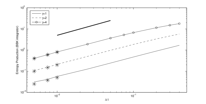
Figure 5. Entropy production rate as a function of time step, $\Delta t$, for various friction factors $\gamma$. The decrease of the entropy production rate is linear as Theorem 78 asserts. Additionally, the theoretically-computed entropy production rate (star points) perfectly matches the numerically-computed entropy rate.

4. Summary and Future Work

In this paper we use the entropy production rate as a novel tool to assess quantitatively the (lack of) reversibility of discretization schemes for various reversible SDE’s. Reversibility of the discrete-time approximation process is a desirable feature when equilibrium simulations are performed. The entropy production rate which is defined as the time-average of the relative entropy between the path measure of the forward process and the path measure of the time-reversed process is zero when the process is reversible and positive when it is irreversible. Thus, it provides a way to quantify the (ir)reversibility of the approximation process. Moreover, under an ergodicity assumption, the entropy production rate can be computed numerically on-the-fly utilizing the GC action functional. This is another attractive feature of the entropy production rate.

We computed the entropy production rate for overdamped Langevin processes both analytically and numerically when discretized with the explicit Euler-Maruyama scheme. One of the main finding in this paper is that depending on the type of the noise –additive vs multiplicative– the entropy production for the explicit EM scheme had totally different behavior. Indeed, for additive noise entropy production rate is of order $O(\Delta t^{2})$ while for multiplicative noise it is of order $O(1)$. Hence, reversibility of the discrete-time approximation process does not depend only on the numerical scheme but also on the intrinsic characteristics of the SDE. For the Milstein’s scheme the entropy production rate $O(\Delta t)$ for multiplicative noise. Furthermore, we computed the entropy production rate both analytically and numerically for discretization schemes of the Langevin process with additive noise. Specifically, we computed the entropy production rate for the BBK integrator of the Langevin equation which is a quasi-symplectic splitting numerical scheme. The rate of entropy production was shown to be of order $O(\Delta t)$.

This paper offers a new conceptual tool for the evaluation of discretization schemes of SDE systems simulated at the equilibrium regime. We consider only the simplest schemes here and we will analyze in future work the behavior of the entropy production for other numerical schemes such as fully implicit EM, drift-implicit EM, higher-order schemes as well as different kind of splitting methods. Moreover, other reversible or even non-reversible processes can be analyzed in the same way, in particular extended, spatially-distributed processes. A particularly interesting example, where the reversibility of the original system is destroyed by numerical schemes in the form of spatio-temporal fractional step approximations of the generator, arises in the (partly asynchronous) parallelization of Kinetic Monte Carlo algorithms [24], [1]. Finally, another possible extension of this work is to develop adaptive schemes based on the a posteriori simulation of entropy production rate, which should guarantee the reversibility or the approximate reversibility of the discrete-time approximation process. In this direction, the decomposition of entropy production functional for Metropolis-adjusted Langevin algorithms (MALA) [21, 12] should be further studied and understood.

Appendix A Tools for proving Theorem 2.1

[Generalized Trapezoidal Rule] For $k$ odd,

$$V(x_{i+1})-V(x_{i}) =\sum_{|\alpha|=1,3,...}^{k}C_{\alpha}[D^{\alpha}V(x_{i+1})+D^{\alpha}V(x_{i})]\Delta x_{i}^{\alpha}$$ (84)

$$+\sum_{|\alpha|=1,3,...}^{k+2}\sum_{|\beta|=k+2-|\alpha|}B_{\beta}[R_{\alpha}^{\beta}(x_{i},x_{i+1})+R_{\alpha}^{\beta}(x_{i+1},x_{i})]\Delta x_{i}^{\alpha+\beta}$$

where $\alpha=(\alpha_{1},...,\alpha_{d})$ is a typical $d$-dimensional multi-index vector, $D^{\alpha}V(x)=\frac{\partial^{|\alpha|}V}{\partial x_{1}^{\alpha_{1}}...\partial x_{d}^{\alpha_{d}}}(x)$ is the $\alpha$-th partial derivative while $x^{\alpha}=x_{1}^{\alpha_{1}}...x_{d}^{\alpha_{d}}$. The coefficients $C_{\alpha}$ are defined recursively by

$$C_{\alpha}=\frac{1}{2}\ \ \ \ \ \ \ \text{for}\ \ \ |\alpha|=1$$ (85)

$$C_{\alpha}=\frac{1}{2}\left(\frac{1}{\alpha!}-\sum_{|\gamma|=1,3,...}^{|\alpha|-2}\frac{1}{(\alpha-\gamma)!}C_{\gamma}\right)\ \ \ \ \ \ \ \text{for}\ \ \ |\alpha|=3,5,...,k$$

while the coefficients $B_{\beta}$ are also recursively defined by

$$B_{\beta}=\frac{1}{2}\ \ \ \ \text{for}\ \ \ |\beta|=0$$ (86)

$$B_{\beta}=-\frac{1}{2}\sum_{|\gamma|=2,4,...}^{|\beta|}\frac{1}{\gamma!}B_{\beta-\gamma}\ \ \ \ \text{for}\ \ \ |\beta|=2,4,...,k+1$$

Finally, the remainder terms are given by
$R_{\alpha}^{\beta}(x_{i},x_{i+1})=\frac{|\alpha|}{\alpha!}\int_{0}^{1}(1-t)^{|\alpha|-1}D^{\alpha+\beta}V((1-t)x_{i}+tx_{i+1})dt$.

Proof.

The starting point is the usual Taylor series expansion around $x_{i}$

$$V(x_{i+1})-V(x_{i})=\sum_{|\alpha|=1}^{k+1}\frac{1}{\alpha!}D^{\alpha}V(x_{i})\Delta x_{i}^{\alpha}+\sum_{|\alpha|=k+2}R_{\alpha}^{0}(x_{i},x_{i+1})\Delta x_{i}^{\alpha}$$ (87)

and around $x_{i+1}$

$$V(x_{i+1})-V(x_{i})=-\sum_{|\alpha|=1}^{k+1}\frac{1}{\alpha!}D^{\alpha}V(x_{i+1})(-\Delta x_{i})^{\alpha}-\sum_{|\alpha|=k+2}R_{\alpha}^{0}(x_{i+1},x_{i})(-\Delta x_{i})^{\alpha}\,.$$ (88)

Adding the two equations we obtain the symmetrized Taylor series expansion for $V$ given by

$$V(x_{i+1})-V(x_{i})=\frac{1}{2}\sum_{|\alpha|=1,3,...}^{k}\frac{1}{\alpha!}[D^{\alpha}V(x_{i+1})+D^{\alpha}V(x_{i})]\Delta x_{i}^{\alpha}$$ (89)

$$-\frac{1}{2}\sum_{|\alpha|=2,4,...}^{k+1}\frac{1}{\alpha!}[D^{\alpha}V(x_{i+1})-D^{\alpha}V(x_{i})]\Delta x_{i}^{\alpha}+\frac{1}{2}\sum_{|\alpha|=k+2}[R_{\alpha}^{0}(x_{i},x_{i+1})+R_{\alpha}^{0}(x_{i+1},x_{i})]\Delta x_{i}^{\alpha}\,.$$

Moreover, generalized trapezoidal formula (84) for $D^{\alpha}V$ with $|\alpha|$ even is

$$D^{\alpha}V(x_{i+1})-D^{\alpha}V(x_{i})=\sum_{|\gamma|=1,3,...}^{k-|\alpha|}C_{\gamma}[D^{\alpha+\gamma}V(x_{i+1})+D^{\alpha+\gamma}V(x_{i})]\Delta x_{i}^{\gamma}$$ (90)

$$+\sum_{|\gamma|=1,3,...}^{k+2-|\alpha|}\sum_{|\beta|=k+2-|\alpha|-|\gamma|}B_{\beta}[R_{\gamma}^{\alpha+\beta}(x_{i},x_{i+1})+R_{\gamma}^{\alpha+\beta}(x_{i+1},x_{i})]\Delta x_{i}^{\beta+\gamma}\,.$$

Hence, substituting (90) into (89), a recursive Taylor series expansion

$$V(x_{i+1})-V(x_{i})=\frac{1}{2}\sum_{|\alpha|=1,3,...}^{k}\frac{1}{\alpha!}[D^{\alpha}V(x_{i+1})+D^{\alpha}V(x_{i})]\Delta x_{i}^{\alpha}$$ (91)

$$-\frac{1}{2}\sum_{|\alpha|=2,4,...}^{k+1}\frac{1}{\alpha!}\sum_{|\gamma|=1,3,...}^{k-|\alpha|}C_{\gamma}[D^{\alpha+\gamma}V(x_{i+1})+D^{\alpha+\gamma}V(x_{i})]\Delta x_{i}^{\alpha+\gamma}$$

$$-\frac{1}{2}\sum_{|\alpha|=2,4,...}^{k+1}\frac{1}{\alpha!}\sum_{|\gamma|=1,3,...}^{k+2-|\alpha|}\sum_{|\beta|=k+2-|\alpha|-|\gamma|}B_{\beta}[R_{\gamma}^{\alpha+\beta}(x_{i},x_{i+1})+R_{\gamma}^{\alpha+\beta}(x_{i+1},x_{i})]\Delta x_{i}^{\alpha+\beta+\gamma}$$

$$+\frac{1}{2}\sum_{|\alpha|=k+2}[R_{\alpha}^{0}(x_{i},x_{i+1})+R_{\alpha}^{0}(x_{i+1},x_{i})]\Delta x_{i}^{\alpha}$$

$$=\frac{1}{2}\sum_{|\alpha|=1,3,...}^{k}\frac{1}{\alpha!}[D^{\alpha}V(x_{i+1})+D^{\alpha}V(x_{i})]\Delta x_{i}^{\alpha}$$

$$-\frac{1}{2}\sum_{|\alpha|=3,5,...}^{k}\sum_{|\gamma|=1,3,...}^{|\alpha|-2}\frac{1}{(\alpha-\gamma)!}C_{\gamma}[D^{\alpha}V(x_{i+1})+D^{\alpha}V(x_{i})]\Delta x_{i}^{\alpha}$$

$$+\frac{1}{2}\sum_{|\alpha|=k+2}\sum_{|\beta|=k+2-|\alpha|}[R_{\alpha}^{\beta}(x_{i},x_{i+1})+R_{\alpha}^{\beta}(x_{i+1},x_{i})]\Delta x_{i}^{\alpha}$$

$$-\frac{1}{2}\sum_{|\alpha|=1,3,...}^{k}\sum_{|\beta|=k+2-|\alpha|}\sum_{|\gamma|=2,4,...}^{|\beta|}\frac{1}{\gamma!}B_{\beta-\gamma}[R_{\alpha}^{\beta}(x_{i},x_{i+1})+R_{\alpha}^{\beta}(x_{i+1},x_{i})]\Delta x_{i}^{\alpha+\beta}$$

is obtained after rearrangements of the sums. Equating the same powers of (LABEL:recursive:Taylor:series) and (84), the coefficients $C_{\alpha}$ and $B_{\beta}$ are obtained.

Thus far, we presented how to compute the coefficients of the generalized trapezoidal formula. A rigorous proof of the lemma is then easily derived by induction on the order, $k$, of (84) and proceeding on the reverse direction of the above formulae. ∎

Assume that the discrete-time Markov process $x_{i}$ driven by

$$x_{i+1}=F(x_{i},\Delta W_{i})$$ (92)

where $\Delta W_{i}$ are i.i.d. Gaussian random variables is ergodic with invariant measure $\bar{\mu}$. Then,

• For sufficiently smooth function $h$ we have

  $$\lim_{n\rightarrow\infty}\frac{1}{n}\sum_{i=0}^{n-1}h(x_{i},\Delta W_{i})=\mathbb{E}_{\bar{\mu}\times\rho}[h(x,y)]\,.$$ (93)

• For sufficiently smooth functions $f$ and $g$ we have

  $$\lim_{n\rightarrow\infty}\frac{1}{n}\sum_{i=0}^{n-1}f(x_{i})g(\Delta W_{i})=\mathbb{E}_{\bar{\mu}}[f(x)]\mathbb{E}_{\rho}[g(y)]\,.$$ (94)

• For sufficiently smooth functions $f$ and $g$ and for bounded $f$ holds that

  $$\lim_{n\rightarrow\infty}\frac{1}{n}\sum_{i=0}^{n-1}f(x_{i},\Delta W_{i})g(\Delta W_{i})=\mathbb{E}_{\bar{\mu}\times\rho}[f(x,y)]\mathbb{E}_{\rho}[g(y)]\,,$$ (95)

  where $\rho$ is the Gaussian measure.

Proof.

Proving (i) is based on showing that the transition density of the joint process $z_{i}=(x_{i},\Delta W_{i})$ exists and it is positive. Both are trivial since the transition density is the product of the two densities which are both positive. Thus, irreducibility for the joint process is proved and in combination with stationarity, the joint process is ergodic. Relation (ii) is a direct consequence of (i) for $h(x,y)=f(x)g(y)$. By denoting $\bar{f}=\mathbb{E}_{\bar{\mu}\times\rho}[f(x,y)]$ and $\bar{g}=\mathbb{E}_{\rho}[g(y)]$, (iii) is proved by applying (i), noting that

$$\left|\frac{1}{n}\sum_{i=0}^{n-1}f(x_{i},\Delta W_{i})g(\Delta W_{i})-\bar{f}\bar{g}\right|$$ (96)

$$=\left|\frac{1}{n}\sum_{i=0}^{n-1}f(x_{i},\Delta W_{i})g(\Delta W_{i})-\frac{1}{n}\sum_{i=0}^{n-1}f(x_{i},\Delta W_{i})\bar{g}+\frac{1}{n}\sum_{i=0}^{n-1}f(x_{i},\Delta W_{i})\bar{g}-\bar{f}\bar{g}\right|$$

$$\leq M|\frac{1}{n}\sum_{i=0}^{n-1}g(\Delta W_{i})-\bar{g}|+|\bar{g}||\frac{1}{n}\sum_{i=0}^{n-1}f(x_{i},\Delta W_{i})-\bar{f}|\,,$$

since $f$ is bounded (i.e., $|f|\leq M$). Hence, sending $n\rightarrow\infty$, (iii) is proved. ∎

References

• [1] G. Arampatzis, M. A. Katsoulakis, P. Plechac, M. Taufer, and L. Xu. Hierarchical fractional-step approximations and parallel kinetic Monte Carlo algorithms. J. Comp. Phys. (accepted), ArXiv e-prints, May 2012.
• [2] V. Bally and D. Talay. The law of the Euler scheme for stochastic differential equations. I. Convergence rate of the density. Monte Carlo Methods Appl., 2:93–128, 1996.
• [3] V. Bally and D. Talay. The law of the Euler scheme for stochastic differential equations. I. Convergence rate of the distribution function. Probab. Theory Related Fields, 104:43–60, 1996.
• [4] A. Brunger, C. B. Brooks, and M. Karplus. Stochastic boundary conditions for molecular dynamics simulations of ST2 water. Chem. Phys. Lett., 105:495–500, 1984.
• [5] G. Gallavotti and E. G. D. Cohen. Dynamical ensembles in nonequilibrium statistical mechanics. Phys. Rev. Lett., 74:2694–2697, 1995.
• [6] C. Gardiner. Handbook of Stochastic Methods: for Physics, Chemistry and the Natural Sciences. Springer, 1985.
• [7] D. T. Gillespie. Markov Processes: An Introduction for Physical Scientists. NewYork: Academic Press, 1992.
• [8] V. Jakšić, C.-A. Pillet, and L. Rey-Bellet. Entropic fluctuations in statistical mechanics: I. classical dynamical systems. Nonlinearity, 24(3):699–763, 2011.
• [9] R. Khasminskii. Stochastic Stability of Differential Equations. Springer, 2nd Edition, 2010.
• [10] P. E. Kloeden and E. Platen. Numerical Solution of Stochastic Differential Equations. Springer-Verlag, 3rd Ed., 1999.
• [11] J. L. Lebowitz and H. Spohn. A Gallavotti-Cohen type symmetry in the large deviation functional for stochastic dynamics. J. Stat. Phys., 95:333–365, 1999.
• [12] T. Lelievre, M. Rousset, and G. Stoltz. Free energy computations: a mathematical perspective. Imperial College Press, 2010.
• [13] C. Maes, F. Redig, and A. Van Moffaert. On the definition of entropy production, via examples. J. Math. Phys., 41:1528–1553, 2000.
• [14] J. C. Mattingly, A.M. Stuart, and M.V. Tretyakov. Convergence of numerical time-averaging and stationary measures via Poisson equations. SIAM J. Numer. Anal., 48:552–577, 2010.
• [15] J.C. Mattingly, A.M. Stuart, and D.J. Higham. Ergodicity for SDEs and approximations: locally Lipschitz vector fields and degenerate noise. Stochastic Processes and their Applications, 101:185–232, 2002.
• [16] S.P. Meyn and R.L. Tweedie. Markov Chains and Stochastic Stability. Springer-Verlag, 1993.
• [17] G. Milstein and M. Tretyakov. Stochastic Numerics for Mathematical Physics. Springer, 2004.
• [18] G. Nicolis and I. Prigogine. Self-Organization in Nonequilibrium Systems. Wiley, New York, 1977.
• [19] L. Rey-Bellet and L.E. Thomas. Exponential convergence to non-equilibrium stationary states in classical statistical mechanics. Comm. Math. Phys., 225(2):305–329, 2002.
• [20] Luc Rey-Bellet. Ergodic properties of Markov processes. In Open quantum systems. II, volume 1881 of Lecture Notes in Math., pages 1–39. Springer, Berlin, 2006.
• [21] G. O. Roberts and R. L. Tweedie. Geometric convergence and central limit theorems for multidimensional Hastings and Metropolis algorithms. Biometrika, 83:95–110, 1996.
• [22] T. Schlick. Molecular Modeling and Simulation. Springer, 2002.
• [23] J. Schnakenberg. Network theory of microscopic and macroscopic behavior of master equation systems. Rev. Modern Phys., 48(4):571–585, 1976.
• [24] Yunsic Shim and Jacques G. Amar. Semirigorous synchronous relaxation algorithm for parallel kinetic Monte Carlo simulations of thin film growth. Phys. Rev. B, 71(12):125432, Mar 2005.
• [25] D. Talay. Second order discretization schemes of stochastic differential systems for the computation of the invariant law. Stochastics Stochastics Rep., 29:13–36, 1990.
• [26] D. Talay. Stochastic Hamiltonian systems: exponential convergence to the invariant measure, and discretization by the implicit Euler scheme. Markov Processes and Related Fields, 8:163–198, 2002.
• [27] D. Talay and L. Tubaro. Expansion of the global error for numerical schemes solving stochastic differential equations. Stoch. Anal. Appl, 8:483–509, 1990.
• [28] N. G. van Kampen. Stochastic Processes in Physics and Chemistry. North Holland, 2006.