The Interval Property in Multiple Testing of Pairwise Differences

Abstract

The usual step-down and step-up multiple testing procedures most often lack an important intuitive, practical, and theoretical property called the interval property. In short, the interval property is simply that for an individual hypothesis, among the several to be tested, the acceptance sections of relevant statistics are intervals. Lack of the interval property is a serious shortcoming. This shortcoming is demonstrated for testing various pairwise comparisons in multinomial models, multivariate normal models and in nonparametric models.

Residual based stepwise multiple testing procedures that do have the interval property are offered in all these cases.

and

1 Introduction

Stepwise multiple testing procedures are valuable because they are less conservative than standard single-step procedures which often rely on Bonferroni critical values. In other words, they are more powerful than their single-step counterparts. In constructing stepwise testing procedures it is common to begin with tests for the individual hypotheses that are known to have desirable properties. For example, the tests may be UMPU, they may have invariance properties and are likely to be admissible. Then a sequential component is added that tells us which hypotheses to accept or reject at each step and when to stop. We begin with the realization that all stepwise procedures induce new tests on the individual testing problems. Carrying out a stepwise procedure in a multiple hypothesis testing problem is equivalent to applying these induced tests separately to the individual hypotheses. Thus, if the induced individual tests can be improved, then the entire procedure is improved. Due to the sequential component, the nature of these induced tests is typically complicated and overlooked. Unfortunately they frequently do not retain all the desirable properties that the original tests possessed.

In this paper we focus on an important type of practical property (which in many models is also a necessary theoretical property) that we call the interval property. This is a desirable property that the original tests would typically have but that the stepwise induced tests can easily lose. Informally the interval property is simply that the resulting test has acceptance sections that are intervals.

To further clarify, suppose one is constructing a test for a one-sided hypothesis testing problem. In addition to asking for other properties it is sensible to examine the acceptance and rejection regions. There are often pairs of sample points, $\mathbf{X}$ and $\mathbf{X}^{\ast}$, for which there are compelling practical (and sometimes theoretical) reasons for the following to be true. If the point $\mathbf{X}$ is in the rejection region, then the point $\mathbf{X}^{\ast}$ should also be in the rejection region. The practical desirability of this property is usually due to the fact that it is intuitively “clear” that $\mathbf{X}^{\ast}$ is a stronger indication of the alternative than is $\mathbf{X}$. In the case of two-sided hypotheses there are often triples of points, $\mathbf{X},\mathbf{X}^{\ast}$ and $\mathbf{X}^{\ast\ast}$ (on the same line), such that if both X and $\mathbf{X}^{\ast\ast}$ are in the acceptance region, then one would also want $\mathbf{X}^{\ast}$ to be in the acceptance region if in fact $\mathbf{X}^{\ast}$ was not the most indicative of the alternative of the three points.

We illustrate this idea with an example that will be treated fully in Section 5.1. Suppose one observes the data in Table 1 based on the three labeled independent treatments. One of the hypotheses of interest is whether or not the distribution for Dose 1 is stochastically larger than that for the placebo. If the method used decides in favor of stochastic order based on observing Table 1, then it should also decide in favor of Dose 1 if Table 2 is observed. Repeated use of a test procedure not having this property will ultimately lead to conclusions that seem contradictory and would be difficult to justify. The interval property is not only natural but is necessary for admissibility. We will return to Tables 1 and 2 later in Section 5.1.

Table 1: Health Status data at sample point $\mathbf{x}$

	Same	Improved	Cured
Placebo	15	226	04	245
Dose 1	04	226	15	245
Dose 2	06	196	43	245

Table 2: Health Status data at sample point $\mathbf{x}^{\bolds{\ast}}$

	Same	Improved	Cured
Placebo	16	226	03	245
Dose 1	03	226	16	245
Dose 2	06	196	43	245

We study this idea in the most common of multiple testing situations, that is, those where hypotheses under consideration involve collections of pairwise differences. The most common of these are(i) treatments versus control problems, (ii) change point problems and (iii) problems examining all pairwise differences. We will investigate these problems in a broad spectrum of models: univariate models involving means or variances, multivariate models concerning mean vectors, ordinal data models involving equality of multinomial distributions and nonparametric models involving equality of distributions.

Two popular types of multiple testing procedures for such problems are a step-down procedure (to be defined later) and a step-up procedure. To simplify the presentation we focus mainly on the step-down procedure as analogous results can be obtained for the FDR controlling step-up procedure of Benjamini and Hochberg (1995). We will see that these step-down induced tests often do not retain the interval property. In fact, among all the models considered the usual step-down procedure maintains the interval property only when testing treatments versus control in the one-sided case. We will also show how to construct a step-down procedure that does have the interval property. Furthermore, it should be clear from the examples and from the way that the methods are used that this phenomenon exists in a far greater variety of models.

The usual step-down procedure is given in Lehmann and Romano (2005). For testing all pairwise comparisons variations are offered in Holm (1979), Shaffer (1986), Royen (1989) and Westfall and Tobias (2007). The lack of the interval property in a one-way ANOVA model for testing all pairwise contrasts is shown in Cohen, Sackrowitz and Chen (2010) (CSC) under a normal model. It has also been demonstrated for rank tests in a one-way ANOVA model in Cohen and Sackrowitz (2012) (CS).

Many multiple testing procedures are designed to control some error rate such as the familywise error rate FWER (weak and strong), the false discovery rate FDR and k-FWER (see (Lehmann and Romano, 2005)). Some researchers also take a finite action decision theory problem approach with a variety of loss functions (e.g., (Genovese and Wasserman, 2002)). In these studies procedures are evaluated and compared by their risk functions. The risk function approach does not always necessitate the need to control a particular type of error rate. Dudoit and Van der Laan (2008) study expected values of functions of numbers of Type I and Type II errors. In any particular application one would typically have a sense of desirable criteria as well as those portions of the parameter space that are most relevant. To get a more complete understanding of the behavior of one’s procedure we recommend that, if feasible, error control and risk function properties should be examined.

In this paper we specify procedures that have the interval property for a much wider class of both univariate and multivariate models. For exponential family models, where individual test statistics are dependent, each individual test induced by usual step-down and step-up procedures has been shown to be inadmissible with respect to the classical hypothesis testing 0–1 loss. See Cohen and Sackrowitz (2005, 2007, 2008) and CSC (2010) cited above.Those proofs are based on results of Matthes and Truax (1967) that, in effect, say that the interval property is equivalent to admissibility. One implication of this is that no Bayesian approach would lead to a procedure that lacks the interval property. Thus no prior distribution can be used to explain a lack of the interval property.

Lack of the interval property not only means that, in exponential family models, procedures exist with both better size and power for every individual hypothesis, but it may also lead to very counterintuitive results. It is hard to believe a client would be happy with a procedure that could yield a reject of a null hypothesis in one instance and then yield an accept of the same hypothesis in another instance when the evidence and intuition is more intuitively compelling in the latter case.

The methodology we present leads to procedures that are admissible. Furthermore, their operating characteristics often compare favorably with theusual step-down procedures. This behavior can be seen from the simulations presented in Cohen, Sackrowitz and Xu (2009) (CSX). In that same paper a family of residual based procedures were defined. The step-down procedures having the interval property that will be presented in this paper stem from those procedures. They are exhibited in special cases in CSC (2010) and CS (2012).

In the models considered here, the Residual based Step-Down procedures, labeled RSD, exhibit two important characteristics. It begins with the set $S=\{1,2,\ldots,k\}$ where each integer is associated with a population. Next, based on all the data, $S$ is partitioned into a collection of disjoint sets through a sequential process. Finally, hypothesis $H_{ij}$ (that population i is equal to population j) is accepted if and only if both $i$ and $j$ are in the same set of the final partition. Second, the partitioning process is based on the pooling of various samples (depending on the particular model at hand) at each stage. The final partition of the set is reached through a sequence of partitions that become finer at each step

There are some noteworthy differences between step-up or step-down and RSD. Depending on the collection of hypotheses being tested, there will be correlation between many of the test statistics being used. Neither step-up nor step-down allows for this in the construction of the test statistic itself. Thus those test statistics will be the same regardless of the correlation structure. The RSD methodology yields statistics that are determined by the correlation structure. Furthermore, the RSD test statistics change at each step depending on the actions taken at the previous step.

Unfortunately, insight as to why the interval property will ensue in some cases but not others is still wanting. The crucial element seems to be the way the test statistics and stopping rules mesh and this must be checked mathematically.

We point out that many of the step-down procedures discussed here are symmetric in the sense that whatever is true for any one hypothesis to be tested is also true for the other hypotheses to be tested. So although the lack of the interval property is shown for one particular testing problem, it is true for all individual problems. This takes on added significance for exponential family models. It means that every individual test is inadmissible. When the number of hypotheses is large, the number of opportunities for inconsistent decisions also gets to be large. For risk functions that would sum mistakes, such as the classification risk ((Genovese and Wasserman, 2002)), this could amount to considerable error.

Lastly, we mention the issue of critical values. The shortcoming of RSD and to some extent all stepwise procedures is in determining sharp critical values. This is particularly true in the face of dependence which is exactly the situations in which usual stepwise procedures tend to lack the interval property. With knowledge (based on practicality) of relevant criteria and relevant portions of the parameter space as focus, one can search for appropriate critical values using simulations. A good first simulation for RSD is to use the critical values suggested in the work of Benjamini and Gavrilov (2009) and modify them if necessary. The standard step-up and step-down procedures do not take dependency into account in choosing a level and can also benefit by using simulation to modify their critical values. As examples, two simulations are given for a simple model in Section 6.3. There we compare RSD and step-up in a treatments versus control setting.

In the next section we give models and definitions. Several models, for which the results of the paper hold, are listed. These include normal models, multinomial models, and arbitrary continuous distribution models treated nonparametrically. Section 3 discusses counterexamples to the interval property. In Section 4 we introduce a step-down method, called RSD, that leads to procedures that do have the interval property. Sections 5, 6 and 7 contain results for multinomial models, multivariate normal models and nonparametric models, respectively.

2 Models and Definitions

Let $\pi_{i},i=1,\ldots,k$, be $k$ independent populations. Data from population $\pi_{i}$ is denoted by a $q\times 1$ vector $\mathbf{X}_{i}$ and $\mathbf{X}$ represents $(\mathbf{X}_{1}^{\prime},\ldots,\mathbf{X}_{k}^{\prime})^{\prime}$.

Hypotheses of interest, for particular (i, j) combinations, are denoted by $H_{ij}\dvtx\pi_{i}=\pi_{j}$ versus $K_{ij}\dvtx\pi_{i}\neq\pi_{j}$ or $K_{ij}\dvtx\pi_{i}<\pi_{j}$. The latter one-sided case can be interpreted as the difference in two scalar parameters in case $\pi_{i}$ is characterized by a single parameter or $<$ can be interpreted as $\pi_{j}$ is stochastically larger than $\pi_{i}$ in case $\pi_{i}$ are multinomial distributions or other distributions not necessarily characterized by parameters. We consider situations where there are at least two connected hypotheses among those to be tested, that is, an $H_{ij},H_{jm}$ or an $H_{ij},H_{im}$. We study the following three problems in the domain of pairwise differences:

1. All pairwise differences. Here $H_{ij}\dvtx\pi_{i}=\pi_{j}$ versus $K_{ij}\dvtx\pi_{i}\neq\pi_{j},$ all $i<j,i,j=1,\ldots,k.$

2. Change point. $H_{i(i+1)}\dvtx\pi_{i}=\pi_{i+1}$ versus $K_{i(i+1)}\dvtx\allowbreak\pi_{i}<\pi_{i+1},i=1,\ldots,k-1,$ where $<$ can mean stochastically less than or if $\pi_{i}$ is characterized by a parameter it simply means that the parameter for population $i$ is less than the parameter for population $i+1.$ Two-sided alternatives can also be considered.

3. Treatments versus control. $H_{ik}\dvtx\pi_{i}=\pi_{k}$ versus $K_{ij}\dvtx\pi_{i}\neq\pi_{k},i=1,\ldots,k-1$.

Problems 1, 2 and 3 will be studied for the following probability models:

1. $\pi_{i}$ are independent multinomial distributions. For problem 2 assume $\pi_{1}\leq\pi_{2}\leq\cdots\leq\pi_{k}$ so that the alternative hypotheses are strict stochastic order.

2. $\pi_{i}$ are independent $p$-variate normal distributions with unknown mean vectors $\bolds{\mu}_{i}$ and known covariance matrix $\Sigma$.

3. Assume $\pi_{i}$ has c.d.f. $F_{i}$ with $F_{i}$ continuous. For problem 2 assume $F_{1}\leq\cdots\leq F_{k}$ so alternatives are strict stochastic order.

The intuitive description of the interval property given in Section 1 will be given a formal interpretation on a case by case basis as follows. In each specific model, when $H_{ij}$ is being tested, a vector $\mathbf{g}_{ij}$ will be identified based on compelling practical (and/or theoretical) considerations so that a nonrandomized test $\varphi_{ij}(\mathbf{x})$ will be said to have the interval property (relative to the identified $\mathbf{g}_{ij}$) if $\varphi_{ij}(\mathbf{x}+a\mathbf{g}_{ij})$

[(ii)]

is nondecreasing as a function of $a$ in the one-sided case,

has a convex acceptance region in $a$ in the two-sided case.

These practical considerations turn out to involve only the data coming from the populations $\pi_{i}$ and $\pi_{j}$ as they are independent of all the other populations. Thus $\mathbf{g}_{ij}$ will be seen to have entries of 0 for all coordinates that do not correspond to data from $\pi_{i}$ or $\pi_{j}$. Let $\widehat{\mathbf{g}}_{ij}$ be the $2q\times 1$ vector consisting of the elements of $\mathbf{g}_{ij}$ that pertain to $\pi_{i}$ and $\pi_{j}$.

Now let $\widehat{T}_{ij}(\mathbf{x}_{i},\mathbf{x}_{j})$ be the two-population test statistic for testing $H_{ij}$ that, when only $(\mathbf{x}_{i},\mathbf{x}_{j})$ are observed, is the basis of the usual step-down procedure. When all of $\mathbf{x}$ is observed we define $T_{ij}(\mathbf{x})=\widehat{T}_{ij}(\mathbf{x}_{i},\mathbf{x}_{j})$. That is, $T_{ij}$ is a function that depends on $\mathbf{x}$ only through $(\mathbf{x}_{i},\mathbf{x}_{j})$.

Also let $\widehat{\psi}_{ij}((\mathbf{x}_{i},\mathbf{x}_{j}))$ be the nonrandomized test function which utilizes $\widehat{T}_{ij}(\mathbf{x}_{i},\mathbf{x}_{j})$. That is, for a one-sided test $\widehat{\psi}_{ij}(\mathbf{x}_{i},\mathbf{x}_{j})=1$ if $\widehat{T}_{ij}((\mathbf{x}_{i},\mathbf{x}_{j}))>C$ and $\widehat{\psi}_{ij}(\mathbf{x}_{i},\mathbf{x}_{j})=0$ otherwise. For a two-sided test $\widehat{\psi}_{ij}(\mathbf{x}_{i},\allowbreak\mathbf{x}_{j})=1$ if $\widehat{T}_{ij}(\mathbf{x}_{i},\mathbf{x}_{j})<C_{L}$ or $\widehat{T}_{ij}(\mathbf{x}_{i},\mathbf{x}_{j})>C_{U}$. Otherwise $\widehat{\psi}_{ij}(\mathbf{x}_{i},\mathbf{x}_{j})=0$.

In the vast majority of multiple testing problems the same two-sample test statistic is used for every $H_{ij}$. To simplify notation we will use this setting. Extension to the general case would follow easily. Thus, when clear, we suppress subscript notation for two-sample functions as follows:

$$\widehat{\mathbf{g}}_{ij} = \widehat{\mathbf{g}},\quad\widehat{T}_{ij}(\mathbf{x}_{i},\mathbf{x}_{j})=\widehat{T}(\mathbf{x}_{i},\mathbf{x}_{j})\quad\mbox{and}$$

$$\widehat{\psi}_{ij}(\mathbf{x}_{i},\mathbf{x}_{j}) = \widehat{\psi}(\mathbf{x}_{i},\mathbf{x}_{j}),\quad\mbox{all }i<j.$$

We will say $\widehat{\psi}(\mathbf{x}_{i},\mathbf{x}_{j})$ has the interval property relative to $\widehat{\mathbf{g}}$ in the two-sample problem if $\widehat{\psi}_{ij}((\mathbf{x}_{i}^{\prime},\mathbf{x}_{j}^{\prime})^{\prime}+a\widehat{\mathbf{g}})$ satisfies (i) and (ii) above.

At this point we describe the usual step-down procedure for multiple testing of a collection of hypotheses $H_{ij}$ based on statistics $\widehat{T}(\mathbf{x}_{i},\mathbf{x}_{j})$. See, for example, Cohen, Sackrowitz and Xu (2009). We describe the procedure for one-sided alternatives. For two-sided alternatives sometimes statistics are absolute values or upper and lower critical values are used. For one-sided alternatives let $K$ be the number of hypotheses to be tested and let $0\leq C_{1}<C_{2}<\cdots<C_{K}$ be critical values. Define the collection of pairs $Q=\{(i,j)\dvtx H_{ij}$ is to be tested$\}$.

[Step 1:]

Let $\widehat{T}_{i_{1},j_{1}}=\max_{(i,j)\in Q}\widehat{T}(\mathbf{x}_{i},\mathbf{x}_{j}).$ If $\widehat{T}_{i_{1},j_{1}}\leq C_{K},$ accept all hypotheses and stop.

If $\widehat{T}_{i_{1},j_{1}}>C_{K},$ reject $H_{i_{1},j_{1}}$ and go to step 2.

Consider $\widehat{T}_{i_{2},j_{2}}\,{=}\,\max_{(i,j)\in Q\setminus(i_{1},j_{1})}\widehat{T}(\mathbf{x}_{i},\mathbf{x}_{j})$. If $\widehat{T}_{i_{2},j_{2}}\leq C_{K-1},$ accept all remaining hypotheses. If $\widehat{T}_{i_{2},j_{2}}>C_{K-1},$ reject $H_{i_{2},j_{2}}$ and go to step 3.

Consider

$$\widehat{T}_{i_{m},j_{m}}=\max_{(i,j)\in Q\setminus\{(i_{1},j_{1})\cdots(i_{m-1},j_{m-1})\}}\widehat{T}(\mathbf{x}_{i},\mathbf{x}_{j}).$$

If $\widehat{T}_{i_{m},j_{m}}\leq C_{K-(m-1)},$ accept all remaining hypotheses.

If $\widehat{T}_{i_{m},j_{m}}>C_{K-(m-1)},$ reject $H_{i_{m},j_{m}}$ and go to step $(m+1)$.

We remark that the RSD methods presented are also based on the function $\widehat{T}$. However, the arguments used are not $(\mathbf{x}_{i},\mathbf{x}_{j})$.

3 Prototype Counterexamples to the Interval Property

In this section we describe the fundamentals of searching for points at which step-down procedures might violate the interval property. The idea is to capitalize on a consequence of the sequential process as follows. Suppose, when $\mathbf{x}$ is observed, the step-down procedure rejects $H_{ij}$ based on the value of $T_{ij}(\mathbf{x})$ but does not do so until stage $m>1$. Further suppose that when $\mathbf{x}^{*}$ is observed there is even more evidence to reject $H_{ij}$ based on $T_{ij}(\mathbf{x}^{*})$. The difficulty is that the stopping rule may prevent the procedure from even reaching stage m when $\mathbf{x}^{*}$ is observed.

To demonstrate we will consider some multiple testing situations using only three populations $\pi_{1}$, $\pi_{2}$, $\pi_{3}$. All the fundamentals can be seen in the case that all $\mathbf{x}_{i}$ are one-dimensional and $T_{ij}=\mathbf{x}_{j}-\mathbf{x}_{i}$ in the one-sided case and $T_{ij}=|\mathbf{x}_{i}-\mathbf{x}_{j}|$ in the two-sided case. Figures 1 and 2 give an intuitive sense of the sort of behavior that one seeks for a violation of the interval property. To extend these ideas to more general situations we use the figures to determine the desired relative positions (with distances measured by the value of the test statistic) of sample points as one moves along the sequence of points $\mathbf{x},\mathbf{x}^{*}\mbox{ and }\mathbf{x}^{**}$.

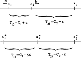
Figure 1: Violation of interval property for one-sided change point problem.

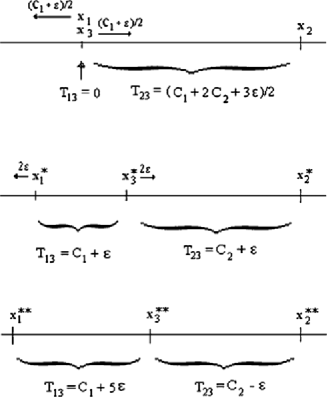
Figure 2: Violation of interval property for two-sided treatments versus control problem.

Figure 1 is appropriate when the (change point) hypotheses to be tested are $H_{12}\dvtx\pi_{1}=\pi_{2}$ versus $K_{12}\dvtx\allowbreak\pi_{1}<\pi_{2}$ and $H_{23}\dvtx\pi_{2}=\pi_{3}$ versus $K_{23}\dvtx\pi_{2}<\pi_{3}$. Suppose $\mathbf{g}_{12}=(-1,1,0)$. When $\mathbf{x}$ is observed $H_{23}$ is rejected at stage 1 and then $H_{12}$ is rejected at stage 2. When $\mathbf{x}^{*}=\mathbf{x}+(2\varepsilon)\mathbf{g}_{12}$ is observed $H_{23}$ is now accepted at stage 1, causing the procedure to stop. Thus $H_{12}$ is now accepted despite an increase in evidence against it.

Figure 2 is appropriate when the (treatments versus control) hypotheses to be tested are $H_{13}\dvtx\pi_{1}=\pi_{3}$ versus $K_{13}\dvtx\pi_{1}\neq\pi_{3}$ and $H_{23}\dvtx\pi_{2}=\pi_{3}$ versus $K_{23}\dvtx\allowbreak\pi_{2}\neq\pi_{3}$. Here $\pi_{3}$ is the control and $\mathbf{g}_{13}=(-1,0,1)$. When $\mathbf{x}$ is observed $H_{23}$ is rejected at stage 1 and then $H_{13}$ is accepted at stage 2. When $\mathbf{x}^{*}=\mathbf{x}+((C_{1}+\varepsilon)/2)\mathbf{g}_{13}$ is observed $H_{23}$ is rejected at stage 1 and then $H_{13}$ is rejected at stage 2. Finally, when $\mathbf{x}^{**}=\mathbf{x}^{*}+(2\varepsilon))\mathbf{g}_{13}$ is observed both hypotheses are accepted. In the sample space as we go from $\mathbf{x}$ to $\mathbf{x}^{*}$ to $\mathbf{x}^{**}$ the evidence against $H_{13}$ continues to mount. Yet the step-down procedure’s decisons are to accept, reject and then accept again on this sequence of points.

Figure 2 is also appropriate when testing all pairwise comparisons provided $C_{1}+2C_{2}>2C_{3}$.

4 RSD Features and First Properties

In this section we describe some specifics of the step-down procedures we will present that do have the interval property. As previously mentioned, decisions are, in effect, based on a final partition of the set $S=\{1,2,\ldots,k\}$ that is reached through a sequence of data based partitions that become finer at each step. Each integer is associated with a population. Suppose the hypothesis $H_{ij}\dvtx\pi_{i}=\pi_{j}$ is under consideration. Then $H_{ij}$ is rejected if and only if $i$ and $j$ are in different sets of the final partition of $S$. The precise rules for the partitioning depend on the model and the data. Illustrative examples of the process will be given at the end of this section. However, certain principles are common to all models.

At the first step the process either stops and $S$ itself is the final partition (in this case no hypothesis can be rejected) or $S$ is divided into two sets. At any future step the process either stops or one of the sets in the current partition is divided into two nonempty sets. The types of allowable sets in the partition process are often restricted by the particular model being considered. For the process to begin we must determine three (model-driven) classes of sets, $\Omega,\Omega_{1}$ and $\Omega_{2}$. At any step only sets that lie in $\Omega$ are eligible to be split. Of course $\Omega$ must contain at least two integers. One way the process will be stopped is if the current partition contains no such sets. Further, if a set $B\in\Omega$ is to be divided into $A$ and $B\setminus A$ we require $A\in\Omega_{1}$ and $B\setminus A\in\Omega_{2}$. It is often the case that $\Omega_{1}=\Omega_{2}$. Whenever a set, say $B=\{i_{1},\ldots,i_{m}\}$, is under consideration to be split into two parts the decision is based on some metric $H(A,B\setminus A;\mathbf{x})$ of set dispersion. Here $H$ is defined only for $A\subset B$ with $A$ and $B\setminus A$ both nonempty. For any set of integers, $A$, define

$$n(A) = \mbox{number of integers in }A\quad\mbox{and}$$

$$Y(A;\mathbf{x}) = \sum_{j\in\mathrm{A}}x_{j}.$$

Due to the pairwise nature of each $H_{ij}$ the functions $H(A,B\setminus A;\mathbf{x})$ used in the various multiple testing problems will be chosen to depend only on the functions $n(\cdot)$ and $Y(\cdot;\mathbf{x})$. Next let, for any $B\subset\Omega$,

$$D(B;\mathbf{x})=\max_{A\subset B,A\subset\Omega_{1},B\setminus A\subset\Omega_{2}}H(A,B\setminus A;\mathbf{x})$$

and let the max be attained for the set $A_{B}$. That is, $D(B;\mathbf{x})=H(A_{B},B\setminus A_{B};\mathbf{x})$. If the set $B$ is ever to be divided, it will be split into $A_{B}$ and $B\setminus A_{B}$. The dependence of $A_{B}$ on $\mathbf{x}$ will usually be suppressed in the notation.

Let $\{C_{m}\},m=1,\ldots,k$ be an increasing set of critical values. Suppose that for some sample point $\mathbf{x}$ stage m is reached and the current partition entering stage m is denoted by $B_{1m},\ldots,B_{mm}$. If

$$\max(D(B_{1m};\mathbf{x}),\ldots,D(B_{mm};\mathbf{x}))>C_{k+1-m}$$

then split the set corresponding to the largest$D(B_{im};\mathbf{x})$ and continue to the next stage. Otherwise stop.

This construction leads to the following two basic results.

Theorem 4.1.

Suppose $H(A,B\setminus A;\mathbf{x}+a\mathbf{g})$ has the following properties. It is [(iii)]

a nondecreasing function of a if $\{i\}\in A,\{j\}\in B\setminus A$ or $\{j\}\in A,\{i\}\in B\setminus A;$

constant as a function of a if $\{i,j\}\subseteq A$ or $\{i,j\}\subseteq B\setminus A;$

constant as a function of a if $\{i,j\}\cap B=\phi.$ If the final partition at the sample point $\mathbf{x}$ places $i$ and $j$ in different sets, then the final partition at $\mathbf{x}^{*}=\mathbf{x}+a\mathbf{g},a>0$ will also place $i$ and $j$ in different sets.

Since the final partition at the point $\mathbf{x}$ placed i and j in different sets, the partitioning process continued, at least, until $i$ and $j$ were separated. Consider any stage in which $i$ and $j$ have not yet been separated. In that partition let $B^{*}$ denote the set containing both $i$ and $j$. By assumptions (i)–(iii), for any $B$ in that same partition we must have $H(A,B\setminus A;\mathbf{x}+a\mathbf{g})=H(A,B\setminus A;\mathbf{x})$ unless $B=B^{*}$ and $\{i\}\in A,\{j\}\in B^{*}\setminus A$ or $\{j\}\in A,\{i\}\in B^{*}\setminus A$. In that case if they are not equal, then [by (i)] we must have $H(A,B^{*}\setminus A;\mathbf{x}+a\mathbf{g})>H(A,B^{*}\setminus A;\mathbf{x})$. Thus i and j would become separated at the point $\mathbf{x}+a\mathbf{g}$ at least as early as they were at the point $\mathbf{x}$. The result now follows.

Theorem 4.2.

Suppose $H(A,B\setminus A;\mathbf{x}+a\mathbf{g})$ has the following properties. It is [(iii)]

nonincreasing and then nondecreasing asa function of a if $\{i\}\in A,\{j\}\in B\setminus A$ or $\{j\}\in A,\allowbreak\{i\}\in B\setminus A;$

constant as a function of a if $\{i,j\}\subseteq A$ or $\{i,j\}\subseteq B\setminus A;$

constant as a function of a if $\{i,j\}\cap B=\phi.$

If the final partition at the sample point $\mathbf{x}$ places $i$ and $j$ in the same set but the final partition at the sample point $\mathbf{x}^{*}=\mathbf{x}+a_{1}\mathbf{g},a_{1}>0$ places $i$ and $j$ in different sets, then the final partition at $\mathbf{x}^{**}=\mathbf{x}+a_{2}\mathbf{g},a_{2}>a_{1}$ will also place $i$ and $j$ in different sets.

Since the final partition at the point $\mathbf{x}$ placed i and j in the same set the partitioning process stopped before i and j were separated. Consider any stage and suppose $B^{*}$ is the set in the partition containing both i and j. By assumptions (i)–(iii), for any $B$ in that partition we must have $H(A,B\setminus A;\break\mathbf{x}\,{+}\,a_{1}\mathbf{g})\,{=}\,H(A,B\setminus A;\mathbf{x})$ unless $B\,{=}\,B^{*}$ and $\{i\}\,{\in}\,A,\break\{j\}\,{\in}\,B^{*}\setminus A$ or $\{j\}\,{\in}\,A,\{i\}\,{\in}\,B^{*}\setminus A$. Since $i$ and $j$ are separated in the final partition at the point $\mathbf{x}+a_{1}\mathbf{g}$ we must have, at some stage, $H(A,B^{*}\setminus A;\allowbreak\mathbf{x}+a_{1}\mathbf{g})>H(A,B^{*}\setminus A;\allowbreak\mathbf{x})$ for some $A$. It now follows from (i) that $H(A,B^{*}\setminus A;\mathbf{x}+a_{2}\mathbf{g})>H(A,B^{*}\setminus A;\allowbreak\mathbf{x}+a_{1}\mathbf{g})$ for this $A$. Hence i and j will be separated at the point $\mathbf{x}+a_{2}\mathbf{g}$ at least as early as they were at $\mathbf{x}+a_{1}\mathbf{g}$.

We conclude this section with some examples of the partitioning process using simple models.

Example 4.1 ((Treatments versus control in a normal model)).

Let $X_{i}\sim N(\mu_{i},1),i=1,2,3,4$ be independent. Let $i=4$ represent the control population and $i=1,2,3$ represent the treatment populations. The objective is to test $H_{i4}\dvtx\mu_{i}=\mu_{4}$ versus $K_{i4}\dvtx\mu_{i}\neq\mu_{4},i=1,2,3$.

To determine an RSD procedure we have opted to begin by taking $\Omega$ to be the collection of all sets containing the integer 4 (control) and at least one other integer chosen from $\{1,2,3\}$. $\Omega_{1}$ is the collection of sets containing exactly one integer from among 1, 2 and 3. $\Omega_{2}$ is the collection of sets containing the integer 4. As our $H(A,B\setminus A;\mathbf{X})$ function we will use

$$H(A,B\setminus A;\mathbf{X})$$

$$\quad=\biggl{|}\sum_{j\in A}X_{j}/n(A)-\sum_{j\in B\setminus A}X_{j}/n(B\setminus A)\biggr{|}\big{/}\tau,$$

where $\tau=\sqrt{1/n(A)+1/n(B\setminus A)}$.

We take our three constants from the Benjamini and Gavrilov (2009) critical values by using the normal distribution with $\alpha=0.05$. That is, $C_{1}=1.48$, $C_{2}=1.97$ and $C_{3}=2.40$. To fix ideas we will take some simple numbers and let $X_{1}=1,X_{2}=4,X_{3}=-2$, $X_{4}=0$.

By our choice of $\Omega_{1}$ one set must contain only one integer and be of the form $A=\{i\}$. Thus at step 1, the RSD procedure considers the following three possible partitions of $S$: [(iii)]

$A=\{1\},S\setminus A=\{2,3,4\},$

$A=\{2\},S\setminus A=\{1,3,4\},$

$A=\{3\},S\setminus A=\{1,2,4\}.$

Thus we have $n(A)=1$ and $n(S\setminus A)=3$ in all three cases. When $A=\{i\}$ the function $H$ becomes

$$H(A,S\setminus A;\mathbf{X})=\biggl{|}X_{i}-\sum_{j\neq i}X_{j}/3\biggr{|}\Big{/}\sqrt{4/3}.$$

In case (i)

$$H = H(\{1\},\{2,3,4\};\mathbf{X})$$

$$= |1-(4-2+0)/3|/\sqrt{4/3}=0.29.$$

In case (ii)

$$H = H(\{2\},\{1,3,4\};\mathbf{X})$$

$$= |4-(1-2+0)/3|/\sqrt{4/3}=3.75.$$

In case (iii)

$$H = H(\{3\},\{1,2,4\};\mathbf{X})$$

$$= |-2-(1+4+0)/3|/\sqrt{4/3}=3.18.$$

The largest of these is 3.75 which is greater than $2.40=C_{3}$. Thus, at step 1, $S$ is split into {2} and $\{1,3,4\}$ and we continue to step 2. Next we consider splitting $B=\{1,3,4\}$ into two parts where the possibilities are

[(iv)]

$A=\{1\}$, and $B\setminus A=\{3,4\},$

$A=\{3\}$, and $B\setminus A=\{1,4\}.$

Thus we have $n(A)=1$ and $n(B\setminus A)=2$ in both cases. When $A=\{i\}$ the function $H$ becomes

$$H(A,B\setminus A;\mathbf{X})=\biggl{|}X_{i}-\sum_{j\neq i}X_{j}/2\biggr{|}\Big{/}\sqrt{3/2}.$$

In case (iv)

$$H = H(\{1\},\{3,4\};\mathbf{X})$$

$$= |1-(-2+0)/2|/\sqrt{3/2}=1.63.$$

In case (v)

$$H = H(\{3\},\{1,4\};\mathbf{X})$$

$$= |-2-(1+0)/2|/\sqrt{3/2}=2.04.$$

The largest of these is 2.04 which is greater than $1.97=C_{2}$. Thus, at step 2, $\{1,3,4\}$ is split into {3} and $\{1,4\}$ and we continue to step 3. At step 3 we consider splitting {1,4} into two parts. $H$ is now simply

$$H=H(\{1\},\{4\};\mathbf{X})=|1-(0)|/\sqrt{2}=0.71.$$

Since $0.71<1.48=C_{1}$ the set $\{1,4\}$ remains intact and the process stops. The final partition is $\{2\}$, $\{3\}$ and $\{1,4\}$. Recalling that if i and j are placed in different sets then $H_{ij}$ will be rejected, we find that $H_{14}$ is accepted, $H_{24}$ is rejected and $H_{34}$ is rejected.

For each (treatment) $i=1,2,3$ in this setting the interval property would pertain to the behavior of the test as $X_{i}$ increased and $X_{k}$ decreased while the other (independent variables) remained fixed. Thus the vector $\mathbf{g}$ would have a $-1$ in the fourth position, a $+1$ in the $i$th position and zeroes elsewhere. It is not difficult to check that the function $H$ given in (4.1) satisfies the conditions of Theorems 1 and 2.

Example 4.2 ((Change point in a normal model)).

Let $X_{i}\sim N(\mu_{i},1),i=1,\ldots,10$, be independent. The objective is to test $H_{i,i+1}\dvtx\mu_{i}=\mu_{i+1}$ versus $K_{i,i+1}\dvtx\break\mu_{i}\neq\mu_{i+1},i=1,\ldots,9$.

To determine an RSD procedure we will begin by taking $\Omega$ to be the collection of all sets containing at least two consecutive integers chosen from $\{1,\ldots,10\}$. $\Omega_{1}$ is the collection of sets containing consecutive integers chosen from among $1,\ldots,9$. $\Omega_{2}$ is the collection of sets containing consecutive integers chosen from $2,\ldots,10$. As our $H(A,B\setminus A;\mathbf{X})$ function we will again use the function defined in Equation (4.1). Now there can be, at most, nine steps in the partition process. Again we can use nine constants coming from the Benjamini and Gavrilov (2009) critical values by using the normal distribution with $\alpha=0.05$.

At step 1 the possible partitions are

$$A=\{1,\ldots,i\},\quad S\setminus A=\{i+1,\ldots,10\}$$

$$\eqntext{\mbox{for }i=1,\ldots,9.}$$ (3)

Proceeding as in Example 4.1 we use the $H$ function and the constant $C_{9}$ to decide if and how to divide $S$. Suppose it is determined (based on the data) to split $S$ into the sets $\{1,\ldots,d\}$ and $\{d+1,\ldots,10\}$ for some $d=1,\ldots,9$. If $d=1$, then at step 2 only $\{2,\ldots,10\}$ is eligible to be split while if $d=9$, only $\{1,\ldots,9\}$ is eligible. However, if $1<d<9$, then both $\{1,\ldots,d\}\mbox{ and }\{d+1,\ldots,10\}$ must be considered at step 2. At step 2 we consider all divisions of the form

$$A=\{1,\ldots,i\},\quad B\setminus A=\{i+1,\ldots,d\}$$

$$\eqntext{\mbox{for }i=1,\ldots,d-1}$$ (4)

and

$$A=\{d+1,\ldots,i\},\quad B\setminus A=\{i+1,\ldots,10\}$$

$$\eqntext{\mbox{for }i=1,\ldots,9.}$$ (5)

Now using the $H$ functions and the constant $C_{8}$ we would determine one which, if any, of the above sets should be split. We continue in this fashion until either there are no more sets eligible to be split or none satisfy the criterion to be split. As in Example 4.1, if i and $i+1$ are placed in different sets of the final partition, then $H_{i,i+1}$ will be rejected.

5 Multinomial Models

In this section we assume that there are $k$ independent multinomial populations each with $q$ cells. Let $\pi_{i},i=1,\ldots,k$ represent the $i$th population with cell probabilities $p_{ij},j=1,\ldots,q$.

The individual testing problems are either $H_{i,j}\dvtx\break\pi_{i}=\pi_{j}$ versus $K_{i,j}\dvtx\pi_{i}<\pi_{j}$ or $H_{i,j}\dvtx\pi_{i}=\pi_{j}$ versus $K_{i,j}\dvtx\pi_{i}\neq\pi_{j}$ where $i<j$. In this case $\pi_{i}<\pi_{j}$ means population $j$ is stochastically larger than population $i$, that is, $\sum_{l=1}^{m}p_{il}\geq\sum_{l=1}^{m}p_{jl}$ for $m=1,\ldots,q$ with some strict inequality.

Let $\widehat{T}(\mathbf{x}_{i},\mathbf{x}_{j})$ be the two-sample test statistics used to test $H_{ij}$ that are to be used in the usual step-down multiple testing procedure. A variety of such test statistics have been recommended. See, for example, Basso et al. (2009) (BPSS). Most such statistics, when used to test $H_{ij}$, not as part of a step-down multiple testing procedure, have the interval property described below.

In this setting it is natural to consider a test’s behavior as $x_{i1}$ and $x_{jq}$ both increase while $x_{iq}$ and $x_{j1}$ both decrease. Such changes in data would suggest to a practitioner an ever-increasing amount of stochastic order. To be precise, suppose $(\mathbf{x}_{i},\mathbf{x}_{j})$ is a reject sample point by virtue of using the two-sample test $\widehat{\varphi}$. Next, for $a>0$, consider any sample point $\mathbf{x}^{\ast}$ where $x_{\alpha,\beta}^{\ast}=x_{\alpha,\beta}+a$ for $(\alpha,\beta)=(i,1)$ and $(\alpha,\beta)=(j,q)$, $x_{\alpha,\beta}^{\ast}=x_{\alpha,\beta}-a$ for $(\alpha,\beta)=(j,1)$ and $(\alpha,\beta)=(i,q)$ and $x_{\alpha,\beta}^{\ast}=x_{\alpha,\beta}$ otherwise. Then $\widehat{\varphi}$ has the interval property if $\widehat{\varphi}$ also rejects at $(\mathbf{x}_{i}^{\ast},\mathbf{x}_{j}^{\ast})$. In other words $(\mathbf{x}_{i}^{\ast},\mathbf{x}_{j}^{\ast})$ is more indicative of stochastic order than $(\mathbf{x}_{i},\mathbf{x}_{j})$. So if $(\mathbf{x}_{i},\mathbf{x}_{j})$ is a reject point, $(\mathbf{x}_{i}^{\ast},\mathbf{x}_{j}^{\ast})$ should also be a reject point.

Here $\widehat{\varphi}$ has the interval property relative to the $2q\times 1$ vector $\widehat{\mathbf{g}}$ with 1 in positions 1 and 2$q$, $-1$ in positions $q$ and $q+1$ and 0 elsewhere. Thus for the multiple testing problem the $kq\times 1$ vector $\mathbf{g}_{ij}$ has the value $+1$ in positions $(i-1)(q)+1$ and $(j)(q)$, the value $-1$ in positions $(i)(q)$ and $(j-1)(q)+1$ and the value 0 in all other positions.

It can be verified that all linear statistics and most nonlinear statistics listed in BPSS (2009), Section 2.2 have this interval property. However, these same statistics used as part of a step-down multiple testing procedure will often lead to induced tests that fail to have the interval property.

5.1 Change Point

In the one-sided change point problem the hypotheses are $H_{i,i+1}\dvtx\pi_{i}\,{=}\,\pi_{i+1}$ versus $K_{i,i+1}\dvtx\pi_{i}\,{<}\,\pi_{i+1}$, $i=1,\ldots,k-1$. That is, in the above $j=i+1$. At this point we will demonstrate a simple search that would often lead to the result that the usual step-down procedure for testing $H_{12}$, for example, will not have the interval property. That is, if $\varphi_{12}$ denotes the induced test of $H_{12}$ for the usual step-down procedure, $\varphi_{12}$ will not have the interval property relative to $\mathbf{g}_{12}$. The only impediment to this type of search is the fact that the data consists of integers in each cell and if sample sizes are small this could be problematic. An example will follow the recipe.

We follow the pattern exhibited in Figure 1 while allowing for the presence of additional hypotheses (i.e., $k$ can be greater than 3). Recall that $T_{i(i+1)}(\mathbf{x})$ depends only on $(\mathbf{x}_{i},\mathbf{x}_{i+1})$. Begin by choosing a sample point $\mathbf{x}=(\mathbf{x}_{1}^{\prime},\mathbf{x}_{2}^{\prime},\ldots,\mathbf{x}_{k}^{\prime})^{\prime}$ so that $T_{i(i+1)}(\mathbf{x})>C_{i},i=3,\ldots,k-1;T_{12}(\mathbf{x})=C_{1}+\varepsilon_{1},T_{23}(\mathbf{x})=C_{2}+\varepsilon_{2},\varepsilon_{1}>0,\varepsilon_{2}>0.$ At $\mathbf{x}$, all hypotheses are rejected by step-down. Next consider points $\mathbf{x}^{*}$ of the form $\mathbf{x}^{*}=\mathbf{x}+a\mathbf{g}$. That is, $\mathbf{x}^{\ast}=(\mathbf{x}_{1}^{\ast\prime},\ldots,\mathbf{x}_{k}^{\ast\prime})^{\prime}$ where $\mathbf{x}_{i}^{\ast}=\mathbf{x}_{i}$ for $i=3,\ldots,k$ but $x_{11}^{\ast}=x_{11}+a$, $x_{1j}^{\ast}=x_{1j}$, $j=2,\ldots,q-1$, $x_{1q}^{\ast}=x_{1q}-a$, $x_{21}^{\ast}=x_{21}-a$, $x_{2j}^{\ast}=x_{2j}$, $j=2,\ldots,q-1$, $x_{2q}^{\ast}=x_{2q}+a$.

We note that for most of the statistics used in BPSS (2009) $T_{12}$ is an increasing function of $a$, $T_{23}$ is a decreasing function of $a$ and $T_{i,i+1}$ for $i\geq 3$ does not change with $a$. Choose $a>0$ so that $T_{23}(\mathbf{x}^{\ast})\leq C_{2}$ and $C_{1}+\varepsilon_{1}<T_{12}(\mathbf{x}^{\ast})<C_{2}$. Hence at $\mathbf{x}^{\ast}$ the step-down procedure would reject $H_{i,i+1}$ for $i\geq 3$, but $H_{12}$ and $H_{23}$ would be accepted. Thus the usual step-down procedure does not have the interval property in this case.

Example 5.1.

Consider three independent multinomial distributions, each with three cells. Test $H_{12}\dvtx\allowbreak\pi_{1}=\pi_{2}$ versus $K_{12}\dvtx\pi_{1}<\pi_{2}$ and $H_{23}\dvtx\pi_{2}=\pi_{3}$ versus $K_{23}\dvtx\pi_{2}<\pi_{3}$. Use Wilcoxon–Mann–Whitney (WMW) test statistics $W_{i(i+1)}$ using midranks. See BPSS (2009). The statistics are then normalized by letting $Z_{i(i+1)}=[W_{i(i+1)}-m(m+n+1)/2]/\sqrt{mn(m+n+1)/12}$,where $m$ and $n$ are the row totals of a two-row table.

For the usual step-down procedure choose constants $C_{1}=1.645$ and $C_{2}=1.96$. The data in Table 1 offers sample point $\mathbf{x}$.

The statistics are $Z_{12}(\mathbf{x})=1.653$ and $Z_{23}(\mathbf{x})=2.006$ leading to rejection of $H_{23}$ followed by rejection of $H_{12}$. Now we simply choose $a=1$ to get the sample point $\mathbf{x}^{\ast}$ corresponding to Table 2. For $\mathbf{x}^{\ast}$, $Z_{12}(\mathbf{x}^{\ast})=1.954$ and $Z_{23}(\mathbf{x}^{\ast})=1.865.$ The usual step-down procedure now accepts both hypotheses at $\mathbf{x}^{\ast}$. Thus the usual step-down procedure with induced test $\varphi_{12}$ for $H_{12}$ does not have the interval property relative to $\mathbf{g}_{12}$ where $\widehat{\mathbf{g}}$ has a 1 in positions 1 and 6, a $-1$ in positions 3 and 4 and 0 elsewhere.

Next we introduce another procedure based on the RSD method that does have the interval property. Informally, the RSD approach will, at each stage, consider collections of $2\times q$ tables formed by collapsing sets of consecutive rows. It will then apply a two-sample test having the interval property to these adaptively formed $2\times q$ tables. In order to make this precise we need only define the function $H$ and the sets $\Omega,\Omega_{1}$ and $\Omega_{2}$. First we take $\Omega$ to be the collection of sets containing at least two consecutive integers and take $\Omega_{1}=\Omega_{2}$ to be the collection of all sets of consecutive integers chosen from $S=\{1,2,\ldots,k\}$. Then for any $\widehat{T}$ having the interval property relative to $\widehat{\mathbf{g}}$ let

$$H(A,B\setminus A;\mathbf{x})=\widehat{T}\bigl{(}Y(A),Y(B\setminus A)\bigr{)},$$

where $Y$ is as defined in Equation (4).

Now we use the current choice of $\mathbf{g}$ along with the definitions of $Y$ and $H$ as well as the fact that $\widehat{\mathbf{T}}$ has the interval property relative to $\widehat{\mathbf{g}}$. This allows us to verify that assumptions (i)–(iii) of Theorem 4.1 are satisfied. Thus we have

Theorem 5.1.

RSD has the interval property.

To demonstrate the use of the RSD methodology here we apply it to the model of Example 5.1.

Example 5.1 ((Continued)).

RSD for the data in Table 1, which represents sample point $\mathbf{x}$, is carried out as follows: First Tables 3 and 4 are formed from Table 1 by averaging frequencies in rows 1 and 2 for Table 3 and averaging rows 2 and 3 for Table 4.

Table 3: Data of Table 1 with first two rows combined

	Same	Improved	Cured
(Placebo${}+{}$Dose 1)${}/{}$2	$9.5$	226	$9.5$	245
Dose 2	$6$	196	$43$	245

Table 4: Data of Table 1 with second two rows combined

	Same	Improved	Cured
Placebo	15	226	04	245
(Dose 1${}+{}$Dose 2)${}/{}$2	05	211	29	245

At step 1, WMW test statistics $W_{12,3}(\mathbf{x})$ and$W_{1,23}(\mathbf{x})$ are calculated using midranks and then converted to normalized statistics $Z_{12,3}(\mathbf{x})$ and$Z_{1,23}(\mathbf{x})$. We calculate $Z_{12,3}(\mathbf{x})=2.78$ and $Z_{1,23}(\mathbf{x})=2.603$. Using critical values $C_{1}=1.645$ and $C_{2}=1.96$ we reject $H_{23}$ at step 1 based on $Z_{12,3}(\mathbf{x})$. At step 2 we test $H_{12}$ by using $W_{12}(\mathbf{x})$ normalized to $Z_{12}(\mathbf{x})=1.653$ and thereby reject $H_{12}$ as well. The sample point $\mathbf{x}^{*}$ is represented by the data in Table 2. Proceeding as above we calculate $Z_{12,3}(\mathbf{x}^{*})=2.78$ and $Z_{1,23}(\mathbf{x}^{*})=2.824$. This leads to rejection of $H_{23}$. Next calculate $Z_{12}(\mathbf{x}^{*})=1.946$ which leads to rejection of $H_{12}$.

5.2 Treatments versus Control

Let $\pi_{k}$ be the control population. The hypotheses are $H_{ik}\dvtx\pi_{i}=\pi_{k}$ versus $K_{ik}\dvtx\pi_{i}\neq\pi_{k},i=1,\ldots,k-1$. Let $T(\mathbf{x}_{i},\mathbf{x}_{k})$ be the two-sample test statistics used for testing $H_{ik}$ that are to be used in the usual step-down testing procedure. A wide variety of such tests are listed in BPSS (2009). When we focus on just one hypothesis testing problem we are again comparing just two populations. Therefore the natural $\widehat{\mathbf{g}}$ is the same as that defined in the beginning of this section. That is, the two-sample interval property is relative to the $2q\times 1$ vector $\widehat{\mathbf{g}}$ with 1 in positions 1 and $2q$, $-1$ in positions $q$ and $q+1$ and 0 elsewhere. For the multiple testing problem the $kq\times 1$ vector $\mathbf{g}_{ik}$ has the value $+1$ in positions $(i-1)(q)+1$ and $(k)(q)$, the value $-1$ in positions $(i)(q)$ and $(k-1)(q)+1$ and the value 0 in all other positions.

To show that the usual step-down procedure does not have the interval property we follow the pattern exhibited in Figure 2 while allowing for the presence of additional hypotheses (i.e., $k$ can be greater than 3). Again the discreteness could create a problem with small sample sizes. Recall that $T_{ik}(\mathbf{x})$ depends only on $(\mathbf{x}_{i},\mathbf{x}_{k})$.

Choose a sample point $\mathbf{x}$ so that $\mathbf{x}_{1}$ and $\mathbf{x}_{k}$ are the same, $\mathbf{x}_{i},i=3,\ldots,k-1$ are such that $T_{ik}(\mathbf{x})$ exceeds $C_{i}$ by a substantial amount, $\mathbf{x}_{2}$ is such that $T_{2k}(\mathbf{x})>C_{1}+C_{2}.$ Thus at $\mathbf{x},H_{2k}$ is accepted. Now choose $\mathbf{x}^{*}$ so that $C_{1}<T_{1k}(\mathbf{x}^{\ast})<C_{2}$, and $T_{2k}(\mathbf{x}^{\ast})=C_{2}+\varepsilon$. This is possible since $T_{1k}$ has the interval property and since $\mathbf{x}_{2}^{\ast}$ is closer to $\mathbf{x}_{k}^{\ast}$ than $\mathbf{x}_{2}$ is to $\mathbf{x}_{k}$. Now at $\mathbf{x}^{\ast}$ the procedure rejects $H_{1k}$ and $H_{2k}$. Finally choose $\mathbf{x}^{\ast\ast}$ so that $T_{2k}(\mathbf{x}^{\ast\ast})\leq C_{2}$ and$T_{1k}(\mathbf{x}^{\ast\ast})\leq C_{2}$. This is possible since $\mathbf{x}^{\ast\ast}$ is such that $\mathbf{x}_{1}^{\ast\ast}$ and $\mathbf{x}_{k}^{\ast\ast}$ are moving further apart while $\mathbf{x}_{2}^{\ast\ast}$ and $\mathbf{x}_{k}^{\ast\ast}$ are moving closer to each other. Thus at $\mathbf{x}_{2}^{\ast\ast}$, $H_{1k}$ and $H_{2k}$ are accepted. This demonstrates that the usual step-down procedure lacks the intervalproperty relative to $\mathbf{g}$.

Now we indicate the RSD method that does have the interval property. Informally, the RSD approach will, at each stage, consider collections of $2\times q$ tables formed by taking one row to be one of the treatments while the other row is the result of combining all other treatments with the control. It will then apply a two-sample test having the interval property to these adaptively formed $2\times q$ tables. In order to make this precise we need only define the function $H$ and the sets $\Omega,\Omega_{1}$ and $\Omega_{2}$. First we take $\Omega$ to be the collection of all sets containing $k$ and at least one other integer chosen from $\{1,2,\ldots,k-1\}$. $\Omega_{1}$ is the collection of sets containing exactly one integer. $\Omega_{2}$ is the collection of sets containing the integer $k$. Then for any $\widehat{T}$ having the interval property relative to $\widehat{\mathbf{g}}$ let

$$H(A,B\setminus A;\mathbf{x})=\widehat{T}\bigl{(}Y(A),Y(B\setminus A)\bigr{)}.$$

Now we use the current choice of $\mathbf{g}$ along with the definitions of $Y$ and $H$ as well as the fact that $\mathbf{T}$ has the interval property relative to $\widehat{\mathbf{g}}$. This allows us to verify that assumptions (i)–(iii) of Theorem 4.2 are satisfied. Thus we have

Theorem 5.2.

RSD has the interval property.

5.3 All Pairwise Differences

The hypotheses are $H_{ij}\dvtx\pi_{i}=\pi_{j}$ versus $K_{ij}\dvtx\pi_{i}\neq\pi_{j},i=1,\ldots,k-1,j=i+1,\ldots,k.$ Once again it can be shown that the usual step-down procedure does not have the interval property in this case. Focusing on $H_{12}$ and utilizing statistics $T_{12}\mbox{ and }T_{23}$ as in the arguments of Section 5.1 will suffice to give the results in this case.

We now offer an RSD procedure that does have the interval property. The basis of this RSD procedure is the PADD procedure for testing all pairwise normal means in CSC (2010). For the multinomial case we describe the procedure now.

Again it suffices to follow the exposition in Section 3. Here we let $\Omega$ be the collection of all sets containing at least two integers. Further let $\Omega_{1}=\Omega_{2}$ be the collection of all nonempty subsets of $S=\{1,2,\ldots,k\}$. Next take

$$H(A,B\setminus A;\mathbf{x})=\widehat{T}\bigl{(}Y(A;\mathbf{x}),Y(B\setminus A;\mathbf{x})\bigr{)},$$

where $\widehat{T}$ is any test statistic for testing independence in a $2\times q$ table that has the interval property relative to $\widehat{\mathbf{g}}$.

The interpretation is as follows: By definition every $Y(A;\mathbf{x})$ will be the result of combining all rows corresponding to indices in $A$. In determining how a set $B$ might be split we look at every possible way to collapse all the rows corresponding to the indices in $B$ into just two rows. Then a test is performed for each resulting $2\times q$ table. For example, if $k=4$ and $B=\{1,2,3,4\}$, then the possible splits are $\{1\}$ and $\{2,3,4\}$, $\{2\}$ and $\{1,3,4\}$, $\{3\}$ and $\{1,2,4\}$, $\{4\}$ and $\{1,2,3\}$, $\{1,2\}$ and $\{3,4\}$, $\{1,3\}$ and $\{2,4\}$ or $\{1,4\}$ and $\{2,3\}$.

With these definitions one can check that assumptions (i)–(iii) of Theorem 4.2 are satisfied. Thus we have

Theorem 5.3.

RSD has the interval property.

6 Multivariate Normal Models

Let $\mathbf{x}_{i},i=1,\ldots,k$, be independent q-variate normal random vectors with mean vectors $\bolds{\mu}_{i}$ and known nonsingular covariance matrix $\Sigma$. All hypotheses are concerned with pairwise differences between mean vectors. In light of this we assume without loss of generality that $\Sigma=\mathrm{I}$. The two-sample test statistic that will serve as the basis for all usual step-down procedures considered to test $H_{ij}\dvtx\bolds{\mu}_{i}=\bolds{\mu}_{j}$ versus $K_{ij}\dvtx\bolds{\mu}_{i}\neq\bolds{\mu}_{j}$ is

$$\widehat{T}(\mathbf{x}_{i},\mathbf{x}_{j})=(\mathbf{x}_{i}-\mathbf{x}_{j})^{\prime}(\mathbf{x}_{i}-\mathbf{x}_{j})/2$$ (6)

which has a chi-squared distribution with q degrees of freedom.

Here a natural form of the interval property is along points

$$\mathbf{x} = (\mathbf{x}_{1}^{\prime},\mathbf{x}_{2}^{\prime},\ldots,\mathbf{x}_{k}^{\prime})^{\prime},$$ (7)

$$\mathbf{x}^{\ast} = \bigl{(}(\mathbf{x}_{1}-r_{1}\mathbf{1})^{\prime},(\mathbf{x}_{2}+r_{1}\mathbf{1})^{\prime},\mathbf{x}_{3}^{\prime},\ldots,\mathbf{x}_{k}^{\prime}\bigr{)}^{\prime},$$ (8)

$$\qquad\mathbf{x}^{\ast\ast} = \bigl{(}(\mathbf{x}_{1}-r_{2}\mathbf{1})^{\prime},(\mathbf{x}_{2}+r_{2}\mathbf{1})^{\prime},\mathbf{x}_{3}^{\prime},\ldots,\mathbf{x}_{k}^{\prime}\bigr{)}^{\prime},$$ (9)

where $0<r_{1}<r_{2}$ and $\mathbf{1}$ is a vector of all 1’s. Thus $\widehat{\mathbf{g}}=(-1,\ldots,-1,1,\ldots,1)^{\prime}$ and $\mathbf{g}$ has entries of $-1$ for coordinates corresponding to population i, 1 for coordinates corresponding to population j and 0 elsewhere.

6.1 All Pairwise Differences

The case of $q=1$ has been studied by CSC (2010). For arbitrary q, the lack of the interval property of the usual step-down procedure is shown by focusing on $H_{12}$ and utilizing statistics $T_{12},T_{23}$ as in the argument of Section 5.1.

At this point we describe an RSD which does have the interval property. Here we let $\Omega$ be the collection of all sets containing at least two integers. Further let $\Omega_{1}=\Omega_{2}$ be the collection of all nonempty subsets of $S=\{1,2,\ldots,k\}$. Next take

$$H(A,B\setminus A;\mathbf{x})$$

$$\quad=\widehat{T}\bigl{(}Y(A;\mathbf{x})/n(A),Y(B\setminus A;\mathbf{x})/n(B\setminus A)\bigr{)}$$

$$\qquad{}/\bigl{(}1/n(A)+1/n(B\setminus A)\bigr{)}.$$

Again the assumptions of Theorem 4.2 can be verified and the interval property established.

6.2 Change Point

The hypotheses are $H_{i(i+1)}\dvtx\bolds{\mu}_{i}=\bolds{\mu}_{i+1}$ versus$K_{i(i+1)}\dvtx\bolds{\mu}_{i}\neq\bolds{\mu}_{i+1},i=1,2,\ldots,k-1$. Test statistics for the usual step-down procedure are $\widehat{T}(\mathbf{x}_{i},\mathbf{x}_{i+1})$ as given in (6). The lack of the interval property for the usual step-down is shown by focusing on $H_{12}$ and utilizing statistics $T_{12}$ and $T_{23}$ as in the argument of Section 5.1. Here again we let $\mathbf{x},\mathbf{x}^{\ast},\mathbf{x}^{\ast\ast}$ be as in (7), (8) and (9).

For RSD we proceed as follows: Take $\Omega$ to be the collection of sets containing at least two consecutive integers and take $\Omega_{1}=\Omega_{2}$ to be the collection of all sets of consecutive integers chosen from $S=\{1,2,\ldots,k\}$ and again choose

$$H(A,B\setminus A;\mathbf{x})$$

$$\quad=\widehat{T}\bigl{(}Y(A;\mathbf{x})/n(A),Y(B\setminus A;\mathbf{x})/n(B\setminus A)\bigr{)}$$

$$\qquad{}/\bigl{(}1/n(A)+1/n(B\setminus A)\bigr{)}.$$

Table 5: Performance of RSD and SU. The mean of the control population is 0.0. Each mean value listed represents five treatments. All unspecified means are equal to 0.0

			Expected number of errors
4-9
Means for treatment number			Type I		Type II		Total		FDR
1-3,4-5,6-7,8-9,10-11
1–5	6–10	11–15	RSD	SU	RSD	SU	RSD	SU	RSD	SU
0.00	0.00	$0.00$	0.1	0.7	$0.0$	$0.0$	$0.1$	$0.7$	0.048	0.045
0.00	0.00	$-2.00$	0.1	0.7	$3.5$	$4.4$	$3.6$	$5.1$	0.046	0.050
0.00	0.00	$-4.00$	0.3	0.8	$0.0$	$0.8$	$0.4$	$1.6$	0.051	0.054
0.00	2.00	$-2.00$	0.3	0.7	$6.0$	$8.8$	$6.2$	$9.5$	0.045	0.044
0.00	2.00	$2.00$	0.2	0.8	$6.8$	$8.5$	$7.0$	$9.2$	0.048	0.044
0.00	2.00	$-4.00$	0.4	1.0	$2.7$	$4.6$	$3.1$	$5.6$	0.049	0.054
0.00	2.00	$4.00$	0.4	0.8	$2.7$	$4.8$	$3.2$	$5.6$	0.048	0.048
0.00	4.00	$-4.00$	0.6	0.9	$0.0$	$1.0$	$0.6$	$1.9$	0.050	0.052
0.00	4.00	$4.00$	0.6	0.9	$0.0$	$1.1$	$0.6$	$2.0$	0.049	0.050
2.00	2.00	$-2.00$	0.4	0.9	$8.1$	$12.8$	$8.5$	$13.7$	0.045	0.048
2.00	2.00	$2.00$	0.4	0.9	$10.0$	$12.3$	$10.3$	$13.2$	0.055	0.045
2.00	2.00	$-4.00$	0.6	0.9	$5.3$	$8.2$	$5.9$	$9.2$	0.051	0.048
2.00	2.00	$4.00$	0.6	0.9	$5.3$	$8.6$	$5.9$	$9.4$	0.034	0.047
2.00	4.00	$-4.00$	0.7	1.1	$2.3$	$4.6$	$3.0$	$5.7$	0.049	0.052
2.00	4.00	$4.00$	0.7	1.0	$2.3$	$4.7$	$3.0$	$5.7$	0.049	0.049
4.00	4.00	$-4.00$	0.8	1.2	$0.0$	$1.1$	$0.8$	$2.3$	0.048	0.050
4.00	4.00	$4.00$	0.8	1.3	$0.0$	$1.3$	$0.9$	$2.6$	0.050	0.055

Once again the assumptions of Theorem 4.2 can be verified and so RSD has the interval property in this case.

Remark 6.1.

For the univariate normal change point problem, MRD is a special case of an RSD procedure. For a numerical simulation study comparing MRD with step-down see Cohen, Sackrowitz and Xu (2009).

6.3 Treatments versus Control

The case $q=1$ is treated in CSX (2009) and the case of arbitrary $q$ was treated in Cohen, Sackrowitz and Xu (2008) (CSX).

The hypotheses are $H_{ik}\dvtx\bolds{\mu}_{i}=\bolds{\mu}_{k}$ versus $K_{ik}\dvtx\bolds{\mu}_{i}\neq\bolds{\mu}_{k}$, $i=1,2,\ldots,k-1$. The usual step-down two-sample statistics at step 1 are $T_{ik}=(\mathbf{x}_{i}-\mathbf{x}_{k})^{\prime}(\mathbf{x}_{i}-\mathbf{x}_{k})/2.$ To determine the RSD procedure we take $\Omega$ to be the collection of all sets containing the integer $k$ and at least one other integer chosen from $\{1,2,\ldots,k-1\}$. $\Omega_{1}$ is the collection of sets containing exactly one integer from among $\{1,\ldots,k-1\}$. $\Omega_{2}$ is the collection of sets containing the integer k. As in Sections 6.1 and 6.2 let

$$H(A,B\setminus A;\mathbf{x})$$

$$\quad=\widehat{T}\bigl{(}Y(A;\mathbf{x})/n(A),Y(B\setminus A;\mathbf{x})/n(B\setminus A)\bigr{)}$$

$$\qquad{}/\bigl{(}1/n(A)+1/n(B\setminus A)\bigr{)}.$$

The RSD we use in this situation is simply the vector analog to the procedure shown in Example 4.1. Now, of course, $q\geq 1$, scalar variables and parameters become vectors and the number of treatments is $k-1$. For the function $H$ we use the vector analog to (4.1) that is given in (6.3). Implementation follows the same steps as in Example 4. The only difference might be in the choice of constants as discussed below.

Here again it can be shown that the usual step-down test of $H_{ik}$ does not have the interval property when $\mathbf{g}=(\mathbf{0},\ldots,\mathbf{0},-\mathbf{1},\mathbf{0},\ldots,\mathbf{0},\mathbf{1})$ with the $-\mathbf{1}$ in the $i$th position while RSD does have the interval property.

We now give two simple examples of how the RSD method might be constructed and used. First we mention that for the standard step-up procedure the Benjamini and Hochberg (1995) constants in the two-sided case are given by

$$C^{\mathrm{BH}}_{i}=\Phi^{-1}\bigl{(}1-(k+1-i)(\alpha/2)/k\bigr{)}.$$ (11)

The constants given in Benjamini and Gavrilov (2009) are

$$C^{\mathrm{BG}}_{i}=\Phi^{-1}\bigl{(}1-i(\alpha/2)/(k+1-i(1-\alpha/2)\bigr{)}.$$ (12)

Table 6: Performance of RSD and SU. The mean of the control population is 0.0. Each mean value listed represents eight treatments. All unspecified means are equal to 0.0

			Expected number of errors
4-9
Means for treatment number			Type I		Type II		Total		FDR
1-3,4-5,6-7,8-9,10-11
1–8	9–16	17–24	RSD	SU	RSD	SU	RSD	SU	RSD	SU
0.00	0.00	$0.00$	0.0	0.5	$0.0$	$0.0$	$0.0$	$0.5$	0.031	0.038
0.00	0.00	$-2.00$	0.1	0.7	$6.1$	$6.9$	$6.2$	$7.6$	0.029	0.046
0.00	0.00	$-4.00$	0.3	0.8	$0.0$	$0.9$	$0.3$	$1.8$	0.031	0.051
0.00	2.00	$-2.00$	0.2	0.8	$9.6$	$13.7$	$9.8$	$14.5$	0.027	0.043
0.00	2.00	$2.00$	0.2	0.8	$12.1$	$13.0$	$12.3$	$13.8$	0.037	0.043
0.00	2.00	$-4.00$	0.4	1.1	$4.5$	$6.7$	$4.9$	$7.8$	0.030	0.051
0.00	2.00	$4.00$	0.4	1.0	$4.6$	$6.9$	$5.0$	$7.9$	0.029	0.048
0.00	4.00	$-4.00$	0.5	1.4	$0.0$	$1.2$	$0.6$	$2.6$	0.030	0.056
0.00	4.00	$4.00$	0.5	1.3	$0.0$	$1.3$	$0.6$	$2.6$	0.030	0.053
2.00	2.00	$-2.00$	0.3	1.0	$13.3$	$19.6$	$13.6$	$20.6$	0.028	0.045
2.00	2.00	$2.00$	0.3	1.0	$19.2$	$18.8$	$19.5$	$19.7$	0.058	0.040
2.00	2.00	$-4.00$	0.5	1.0	$9.4$	$12.1$	$9.9$	$13.1$	0.034	0.045
2.00	2.00	$4.00$	0.5	1.0	$9.4$	$12.5$	$10.0$	$13.5$	0.034	0.045
2.00	4.00	$-4.00$	0.6	1.3	$3.8$	$6.5$	$4.5$	$7.8$	0.030	0.048
2.00	4.00	$4.00$	0.6	1.2	$3.8$	$6.7$	$4.5$	$7.9$	0.029	0.046
4.00	4.00	$-4.00$	0.8	1.4	$0.0$	$1.3$	$0.8$	$2.7$	0.030	0.047
4.00	4.00	$4.00$	0.8	1.6	$0.0$	$1.4$	$0.8$	$3.0$	0.030	0.052

Take $q=1$ and $k=101$ so we have 100 treatments and one control. Suppose further that the only reasonable scenario is that the number of truly significant treatments is sparse, say, at the very most, 15% of the treatments. Table 5 gives the results of a simulation using 5000 iterations at each parameter point. We compare the RSD method with step-up on the criteria of FDR, the expected number of Type I errors and the expected number of Type II errors. For RSD we were able to use the critical values of (12) with $\alpha=0.05$ without any modification. For step-up, on the other hand, using $\alpha=0.05$ in (11) resulted in a procedure that was (due to the dependence) too conservative and put it at a disadvantage. Instead we found, using simulation, that taking $\alpha=0.07$ in (11) gave a better performing procedure for this covariance structure. For this application RSD has the interval property, is comparable to step-up relative to FDR and makes fewer mistakes than step-up. Table 6 allows for a less sparse situation allowing as many as 24% better treatments. Here simulation indicated that we should again take $\alpha=0.07$ in (11) for step-up and the critical values of RSD should correspond to $\alpha=0.03$ in (12).

In both Tables 5 and 6 the mean of the control population is taken to be 0.0. In Table 5 the means given in the first three columns each represent five treatment means. The other 85 treatment means are 0.0. For example, in the next to last row, the first 10 treatment means would be 4.00 and the next five treatment means would be $-4.00$. In this case 15% of the treatments would be nonzero. In Table 6 the means given in the first three columns each represent eight treatment means. Thus the maximum number of nonzero treatment means would be, at most, 24%. Note both Tables 5 and 6 indicate fewer errors for RSD for all parameter points considered.

Remark 6.2.

For the univariate normal treatments versus control problem MRD is a special case and natural choice of an RSD procedure. One of the simulation studies in Cohen, Sackrowitz and Xu (2009) was done for this same model but for many more treatments. Both step-up and step-down were considered. As described in that paper it was more difficult to arrive at appropriate choices for critical values. The nature of the results was the same but, due to the large number of populations, the results were stronger.

7 Nonparametric Models

Nonparametric multiple testing is discussed inHochberg and Tamhane (1987). Here we begin with $n$ independent observations from each of $k$ independent populations $F_{1},\ldots,F_{k}$. The collection of all nk observations are ranked and we let $R_{i}=$ the average of the ranks for the observations coming from population $i$. Also let $\mathbf{R}=(R_{1},\ldots,R_{k})^{\prime}$. For testing $H_{ij}\dvtx F_{i}=F_{j}$ versus $K_{ij}\dvtx F_{i}<F_{j}$ or $H_{ij}\dvtx F_{i}=F_{j}$ versus $K_{ij}\dvtx F_{i}\neq F_{j}$ based on $\mathbf{R}$ it is natural to study the behavior of testing procedures as $R_{i}$ decreases and $R_{j}$ increases.

This model fits our original setting with $R_{i}$ playing the role of $\mathbf{x}_{i}$ and $q=1$. Here $\widehat{\mathbf{g}}=(-1,1)^{\prime}$ and $\mathbf{g}$ is the $k\times 1$ vector with $-1$ as the $i$th coordinate, 1 as the $j$th coordinate and 0 elsewhere.

7.1 All Pairwise Differences

The problem of nonparametric multiple testing of all pairwise comparisons of distributions has been treated by Cohen and Sackrowitz (2012) (CS). There it is shown that the step-down procedure of Campbell and Skillings (1985) based on ranks lacks an interval property. It is also shown in CS (2010) that the RSD procedure (called RPADD there) does have the interval property.

7.2 Change Point

Next we consider testing $H_{i(i+1)}\dvtx F_{i}=F_{i+1}$ versus $K_{i(i+1)}\dvtx F_{i}<F_{i+1},i=1,\ldots,k-1$ assuming $F_{i}\leq F_{2}\leq\cdots\leq F_{k}$. Assume sample sizes are $n$ for each population. It is possible to show that a typical step-down procedure using two-sample rank tests (based on separate ranks or joint ranks) for $H_{i(i+1)}$ would not have the interval property. However, the RSD procedure which we now describe will have the interval property. As in the other change point settings, take $\Omega$ to be the collection of sets containing at least two consecutive integers and take $\Omega_{1}=\Omega_{2}$ to be the collection of all sets of consecutive integers chosen from $S=\{1,2,\ldots,k\}.$ Here we let

$$H(A,B\setminus A;\mathbf{R})$$

$$\quad=\bigl{(}Y(A;\mathbf{R})/N(A)$$

$$\hskip 2.0pt\qquad{}-Y(B\setminus A;\mathbf{R})/N(B\setminus A)\bigr{)}/\sigma_{A,B},$$

where

$$\sigma_{A,B}^{2} = w\bigl{(}1/N(A)+1/N(B\setminus A)\bigr{)}/12\quad\mbox{and}$$

$$w = k(kn+1).$$

With these definitions it is easy to verify the conditions of Theorem 4.1 to obtain

Theorem 7.1.

RSD has the interval property for testing $H_{i,i+1}.$

7.3 Treatments versus Control

For testing treatments versus control the hypotheses are $H_{ik}\dvtx F_{i}=F_{k}$ versus $K_{ik}\dvtx F_{i}\neq F_{k}$. Now consider the usual step-down procedure which is based on the two-population statistic

$$T_{ik}=|R_{i}-R_{k}|/\sigma_{\{i\},\{k\}}$$

in comparing the $i$th treatment with the control. It can be shown that the usual step-down procedure does not have the interval property for testing $H_{ik}$.

On the other hand, it can be shown that the RSD procedure for this model does have the interval property for testing $H_{ik}$. RSD in this case is defined as follows: Let $\Omega$ be the collection of all sets containing $k$ and at least one other integer chosen from $S=\{1,2,\ldots,k-1\}$. $\Omega_{1}$ is the collection of sets containing exactly one integer. $\Omega_{2}$ is the collection of sets containing the integer k. Then take

$$H(A,B\setminus A;\mathbf{R})$$

$$\quad=\bigl{|}Y\bigl{(}A;\mathbf{R}/N(A)\bigr{)}$$

$$\hskip 2.0pt\qquad{}-Y(B\setminus A;\mathbf{R})/N(B\setminus A)\bigr{|}/\sigma_{A,B},$$

where $\sigma_{A,B}^{2}$ is as defined in Section 7.2 above. With these definitions it is easy to verify the conditions of Theorem 4.1 to obtain

Theorem 7.2.

RSD has the interval property for testing $H_{i,k}.$

References

- Basso et al. (2009) {bbook}[auto:STB—2012/01/18—07:48:53] \bauthor\bsnmBasso, \bfnmD.\binitsD., \bauthor\bsnmPesarin, \bfnmF.\binitsF., \bauthor\bsnmSalmaso, \bfnmL.\binitsL. and \bauthor\bsnmSolari, \bfnmA.\binitsA. (\byear2009). \btitlePermutation Tests for Stochastic Ordering and Anova. \bpublisherSpringer, \baddressNew York. \bptokimsref \endbibitem
- Benjamini and Gavrilov (2009) {barticle}[mr] \bauthor\bsnmBenjamini, \bfnmYoav\binitsY. and \bauthor\bsnmGavrilov, \bfnmYulia\binitsY. (\byear2009). \btitleA simple forward selection procedure based on false discovery rate control. \bjournalAnn. Appl. Stat. \bvolume3 \bpages179–198. \biddoi=10.1214/08-AOAS194, issn=1932-6157, mr=2668704 \bptokimsref \endbibitem
- Benjamini and Hochberg (1995) {barticle}[mr] \bauthor\bsnmBenjamini, \bfnmYoav\binitsY. and \bauthor\bsnmHochberg, \bfnmYosef\binitsY. (\byear1995). \btitleControlling the false discovery rate: A practical and powerful approach to multiple testing. \bjournalJ. Roy. Statist. Soc. Ser. B \bvolume57 \bpages289–300. \bidissn=0035-9246, mr=1325392 \bptokimsref \endbibitem
- Campbell and Skillings (1985) {barticle}[mr] \bauthor\bsnmCampbell, \bfnmGregory\binitsG. and \bauthor\bsnmSkillings, \bfnmJohn H.\binitsJ. H. (\byear1985). \btitleNonparametric stepwise multiple comparison procedures. \bjournalJ. Amer. Statist. Assoc. \bvolume80 \bpages998–1003. \bidissn=0162-1459, mr=0819606 \bptokimsref \endbibitem
- Cohen and Sackrowitz (2005) {barticle}[mr] \bauthor\bsnmCohen, \bfnmArthur\binitsA. and \bauthor\bsnmSackrowitz, \bfnmHarold B.\binitsH. B. (\byear2005). \btitleCharacterization of Bayes procedures for multiple endpoint problems and inadmissibility of the step-up procedure. \bjournalAnn. Statist. \bvolume33 \bpages145–158. \biddoi=10.1214/009053604000000986, issn=0090-5364, mr=2157799 \bptokimsref \endbibitem
- Cohen and Sackrowitz (2007) {barticle}[mr] \bauthor\bsnmCohen, \bfnmArthur\binitsA. and \bauthor\bsnmSackrowitz, \bfnmHarold B.\binitsH. B. (\byear2007). \btitleMore on the inadmissibility of step-up. \bjournalJ. Multivariate Anal. \bvolume98 \bpages481–492. \biddoi=10.1016/j.jmva.2006.02.002, issn=0047-259X, mr=2293009 \bptokimsref \endbibitem
- Cohen and Sackrowitz (2008) {barticle}[mr] \bauthor\bsnmCohen, \bfnmArthur\binitsA. and \bauthor\bsnmSackrowitz, \bfnmHarold B.\binitsH. B. (\byear2008). \btitleMultiple Testing of two-sided alternatives with dependent data. \bjournalStatist. Sinica \bvolume18 \bpages1593–1602. \bidissn=1017-0405, mr=2469325 \bptokimsref \endbibitem
- Cohen and Sackrowitz (2012) {bmisc}[auto:STB—2012/01/18—07:48:53] \bauthor\bsnmCohen, \bfnmA.\binitsA. and \bauthor\bsnmSackrowitz, \bfnmH. B.\binitsH. B. (\byear2012). \bhowpublishedMultiple Rank Test for Pairwise Comparisons. IMS Collections. To appear. \bptokimsref \endbibitem
- Cohen, Sackrowitz and Chen (2010) {bmisc}[auto:STB—2012/01/18—07:48:53] \bauthor\bsnmCohen, \bfnmA.\binitsA., \bauthor\bsnmSackrowitz, \bfnmH. B.\binitsH. B. and \bauthor\bsnmChen, \bfnmC.\binitsC. (\byear2010). \bhowpublishedMultiple testing of pairwise comparisons. In Borrowing Strength: Theory Powering Applications—A Festschrift for Lawwrence D. Brown. IMS Collections 6 144–157. IMS, Beachwood, OH. \bptokimsref \endbibitem
- Cohen, Sackrowitz and Xu (2008) {barticle}[mr] \bauthor\bsnmCohen, \bfnmArthur\binitsA., \bauthor\bsnmSackrowitz, \bfnmH. B.\binitsH. B. and \bauthor\bsnmXu, \bfnmMinya\binitsM. (\byear2008). \btitleThe use of an identity in Anderson for multivariate multiple testing. \bjournalJ. Statist. Plann. Inference \bvolume138 \bpages2615–2621. \biddoi=10.1016/j.jspi.2008.03.004, issn=0378-3758, mr=2439974 \bptokimsref \endbibitem
- Cohen, Sackrowitz and Xu (2009) {barticle}[mr] \bauthor\bsnmCohen, \bfnmArthur\binitsA., \bauthor\bsnmSackrowitz, \bfnmHarold B.\binitsH. B. and \bauthor\bsnmXu, \bfnmMinya\binitsM. (\byear2009). \btitleA new multiple testing method in the dependent case. \bjournalAnn. Statist. \bvolume37 \bpages1518–1544. \biddoi=10.1214/08-AOS616, issn=0090-5364, mr=2509082 \bptokimsref \endbibitem
- Dudoit and Van der Laan (2008) {bbook}[mr] \bauthor\bsnmDudoit, \bfnmSandrine\binitsS. and \bauthor\bparticlevan der \bsnmLaan, \bfnmMark J.\binitsM. J. (\byear2008). \btitleMultiple Testing Procedures with Applications to Genomics. \bpublisherSpringer, \baddressNew York. \biddoi=10.1007/978-0-387-49317-6, mr=2373771 \bptokimsref \endbibitem
- Genovese and Wasserman (2002) {barticle}[mr] \bauthor\bsnmGenovese, \bfnmChristopher\binitsC. and \bauthor\bsnmWasserman, \bfnmLarry\binitsL. (\byear2002). \btitleOperating characteristics and extensions of the false discovery rate procedure. \bjournalJ. R. Stat. Soc. Ser. B Stat. Methodol. \bvolume64 \bpages499–517. \biddoi=10.1111/1467-9868.00347, issn=1369-7412, mr=1924303 \bptokimsref \endbibitem
- Hochberg and Tamhane (1987) {bbook}[mr] \bauthor\bsnmHochberg, \bfnmYosef\binitsY. and \bauthor\bsnmTamhane, \bfnmAjit C.\binitsA. C. (\byear1987). \btitleMultiple Comparison Procedures. \bpublisherWiley, \baddressNew York. \biddoi=10.1002/9780470316672, mr=0914493 \bptokimsref \endbibitem
- Holm (1979) {barticle}[mr] \bauthor\bsnmHolm, \bfnmSture\binitsS. (\byear1979). \btitleA simple sequentially rejective multiple test procedure. \bjournalScand. J. Statist. \bvolume6 \bpages65–70. \bidissn=0303-6898, mr=0538597 \bptokimsref \endbibitem
- Lehmann and Romano (2005) {bbook}[mr] \bauthor\bsnmLehmann, \bfnmE. L.\binitsE. L. and \bauthor\bsnmRomano, \bfnmJoseph P.\binitsJ. P. (\byear2005). \btitleTesting Statistical Hypotheses, \bedition3rd ed. \bpublisherSpringer, \baddressNew York.\bidmr=2135927 \bptokimsref \endbibitem
- Matthes and Truax (1967) {barticle}[mr] \bauthor\bsnmMatthes, \bfnmT. K.\binitsT. K. and \bauthor\bsnmTruax, \bfnmD. R.\binitsD. R. (\byear1967). \btitleTests of composite hypotheses for the multivariate exponential family. \bjournalAnn. Math. Statist. \bvolume38 \bpages681–697. \bidissn=0003-4851, mr=0208745 \bptokimsref \endbibitem
- Royen (1989) {barticle}[mr] \bauthor\bsnmRoyen, \bfnmTh.\binitsT. (\byear1989). \btitleGeneralized maximum range tests for pairwise comparisons of several populations. \bjournalBiometrical J. \bvolume31 \bpages905–929. \bidissn=0323-3847, mr=1054514 \bptokimsref \endbibitem
- Shaffer (1986) {barticle}[auto:STB—2012/01/18—07:48:53] \bauthor\bsnmShaffer, \bfnmJ. P.\binitsJ. P. (\byear1986). \btitleModified sequantially rejective multiple test procedures. \bjournalJ. Amer. Statist. Assoc. \bvolume81 \bpages826–831. \bptokimsref \endbibitem
- Westfall and Tobias (2007) {barticle}[mr] \bauthor\bsnmWestfall, \bfnmPeter H.\binitsP. H. and \bauthor\bsnmTobias, \bfnmRandall D.\binitsR. D. (\byear2007). \btitleMultiple testing of general contrasts: Truncated closure and the extended Shaffer-Royen method. \bjournalJ. Amer. Statist. Assoc. \bvolume102 \bpages487–494. \biddoi=10.1198/016214506000001338, issn=0162-1459, mr=2325112 \bptokimsref \endbibitem