Joint Specification of Model Space and Parameter Space Prior Distributions

Abstract

We consider the specification of prior distributions for Bayesian model comparison, focusing on regression-type models. We propose a particular joint specification of the prior distribution across models so that sensitivity of posterior model probabilities to the dispersion of prior distributions for the parameters of individual models (Lindley’s paradox) is diminished. We illustrate the behavior of inferential and predictive posterior quantities in linear and log-linear regressions under our proposed prior densities with a series of simulated and real data examples.

abstractwidth345pt keywordwidth345pt

, and

1 Introduction and Motivation

A Bayesian approach to inference under model uncertainty proceeds as follows. Suppose that the data $\mathbf{y}$ are considered to have been generated by a model $m$, one of a set $M$ of competing models. Each model specifies the distribution of $\mathbf{Y}$, $f(\mathbf{y}|m,\allowbreak\bolds{\beta}_{m})$ apart from an unknown parameter vector $\bolds{\beta}_{m}\in B_{m}$, where $B_{m}$ is the set of all possible values for the coefficients of model $m$. We assume that $B_{m}=\mathcal{R}^{d_{m}}$ where $d_{m}$ is the dimensionality of $\bolds{\beta}_{m}$.

If $f(m)$ is the prior probability of model $m$, then the posterior probability is given by

$$f(m|\mathbf{y})={{{f(m)f(\mathbf{y}|m)}}\over{\sum\limits_{m\in M}f(m)f(\mathbf{y}|m)}},\quad m\in M,$$ (1)

where $f(\mathbf{y}|m)$ is the marginal likelihood calculated using $f(\mathbf{y}|m)=\int f(\mathbf{y}|m,\bolds{\beta}_{m})f(\bolds{\beta}_{m}|m)\,d\bolds{\beta}_{m}$ and$f(\bolds{\beta}_{m}|m)$ is the conditional prior distribution of $\bolds{\beta}_{m}$, the model parameters for model $m$. Therefore

$$f(m|\mathbf{y})\propto{f(m)f(\mathbf{y}|m)},\quad m\in M.$$

For any two models $m_{1}$ and $m_{2}$, the ratio of the posterior model probabilities (posterior odds in favor of $m_{1}$) is given by

$$\frac{f(m_{1}|\mathbf{y})}{f(m_{2}|\mathbf{y})}=\frac{f(m_{1})}{f(m_{2})}\frac{f(\mathbf{y}|m_{1})}{f(\mathbf{y}|m_{2})},$$ (2)

the ratio of prior probabilities multiplied by the ratio of marginal likelihoods, also known as the Bayes factor.

The posterior distribution for the parameters of a particular model is given by the familiar expression

$$f(\bolds{\beta}_{m}|m,\mathbf{y})\propto f(\bolds{\beta}_{m}|m)f(\mathbf{y}|\bolds{\beta}_{m},m),\quad m\in M.$$

For a single model, a highly diffuse prior on the model parameters is often used (perhaps to represent ignorance). Then the posterior density takes the shape of the likelihood and is insensitive to the exact value of the prior density function, provided that the prior is relatively flat over the range of parameter values with nonnegligible likelihood. When multiple models are being considered, however, the use of such a prior may create an apparent difficulty. The most obvious manifestation of this occurs when we are considering two models $m_{1}$ and $m_{2}$ where $m_{1}$ is completely specified (no unknown parameters) and $m_{2}$ has parameter $\bolds{\beta}_{m_{2}}$ and associated prior density $f(\bolds{\beta}_{m_{2}}|m_{2})$. Then, for any observed data $\mathbf{y}$, the Bayes factor in favor of $m_{1}$ can be made arbitrarily large by choosing a sufficiently diffuse prior distribution for $\bolds{\beta}_{m_{2}}$ (corresponding to a prior density $f(\bolds{\beta}_{m_{2}}|m_{2})$ which is sufficiently small over the range of values of $\bolds{\beta}_{m_{2}}$ with nonnegligible likelihood). Hence, under model uncertainty, two different diffuse prior distributions for model parameters might lead to essentially the same posterior distributions for those parameters, but very different Bayes factors.

This result was discussed by Lindley (1957) and is often referred to as “Lindley’s paradox” although it is also variously attributed to Bartlett (1957) and Jeffreys (1961). As Dawid (2011) pointed out, the Bayes factor is only one of the two elements on the right side of (2) which contribute toward the posterior model probabilities. The prior model probabilities are of equal significance. By focusing on the impact of the prior distributions for model parameters on the Bayes factor, there is an implicit understanding that the prior model probabilities are specified independently of these prior distributions. This is often the case in practice, where a uniform prior distribution over models is commonly adopted, as a reference position. Examples where nonuniform prior distributions have been suggested include the works of Madigan et al. (1995), Chipman (1996), Laud and Ibrahim (1995, 1996), Chipman, George and McCulloch (2001), Cui and George (2008), Ley and Steel (2009) and Wilson et al. (2010). We propose a different approach where we consider how the two elements of the prior distribution under model uncertainty might be jointly specified so that perceived problems with Bayesian model comparison can be avoided. This leads to a nonuniform specification for the prior distribution over models, depending directly on the prior distributions for model parameters.

A related issue concerns the use of improper prior distributions for model parameters. Such prior distributions involve unspecified constants of proportionality, which do not appear in posterior distributions for model parameters but do appear in the marginal likelihood for any model and in any associated Bayes factors, so these quantities are not uniquely determined. There have been several attempts to address this issue, and to define an appropriate Bayes factor for comparing models with improper priors; see Kadane and Lazar (2004) for a review. In such examples, Dawid (2011) proposed that the product of the prior model “probability” and the prior density for a given model could be determined simultaneously by eliciting the relative prior “probabilities” of particular sets of parameter values for different models. He also suggested an approach for constructing a general noninformative prior, over both models and model parameters, based on Jeffreys priors for individual models. Although the prior distributions for individual models are not generally proper, they have densities which are uniquely determined and hence the posterior distribution over models can be evaluated. Clyde (2000) proposed a similar approach where the priors for parameters of individual models are uniform and the relative weights of different models are chosen by constraining the resulting posterior model probabilities to be equivalent to those resulting from a specified information criterion, such as BIC.

Here, we do not consider improper prior distributions for the model parameters, but our approach is similar in spirit as we do explicitly consider a joint specification of the prior over models and model parameters.

We focus on models in which the parameters are sufficiently homogeneous (perhaps under transformation) so that a multivariate normal prior density $N(\bolds{\mu}_{m},V_{m})$ is appropriate, and in which the likelihood is sufficiently regular for standard asymptotic results to apply. Examples are linear regression models, generalized linear models and standard time series models. In much of what follows, with minor modification, the normal prior can be replaced by any elliptically symmetric prior density proportional to $|V|^{-1/2}g((\bolds{\beta}-\bolds{\mu})^{T}V^{-1}(\bolds{\beta}-\bolds{\mu}))$ where$\int_{0}^{\infty}r^{d-1}g(r^{2})\,dr<\infty$ and $d$ is the dimensionality of $\bolds{\beta}$. This includes prior distributions from the multivariate $t$ or Laplace families. Similarly, our approach can also be adapted to common prior distributions for parameters of graphical models.

We choose to decompose the prior variance matrix as $V_{m}=c_{m}^{2}\Sigma_{m}$ where $c_{m}$ represents the scale of the prior dispersion and $\Sigma_{m}$ is a matrix with a specified value of $|\Sigma_{m}|$, although for the remainder of this section we do not require an explicit value; further discussion of this issue is presented in Section 2. Hence, suppose that

$$f(\bolds{\beta}_{m}|m)$$

$$\quad=(2\pi)^{-d_{m}/2}|\Sigma_{m}|^{-1/2}c_{m}^{-d_{m}}$$ (3)

$$\qquad{}\cdot\exp\biggl{(}-\frac{1}{2c_{m}^{2}}(\bolds{\beta}_{m}-\bolds{\mu}_{m})^{T}\Sigma_{m}^{-1}(\bolds{\beta}_{m}-\bolds{\mu}_{m})\biggr{)}.$$

Then,

$$f(m|\mathbf{y}) \propto f(m)\int f(\mathbf{y}|m,\bolds{\beta}_{m})f(\bolds{\beta}_{m}|m)\,d\bolds{\beta}_{m}$$

$$= f(m)(2\pi)^{-d_{m}/2}|\Sigma_{m}|^{-1/2}c_{m}^{-d_{m}}$$

$${}\cdot\int_{\mathcal{R}^{d_{m}}}\exp\biggl{(}-\frac{1}{2c_{m}^{2}}(\bolds{\beta}_{m}-\bolds{\mu}_{m})^{T}\Sigma_{m}^{-1}$$

$${}\hphantom{\int_{\mathcal{R}^{d_{m}}}\exp\biggl{(}}\cdot(\bolds{\beta}_{m}-\bolds{\mu}_{m})\biggr{)}f(\mathbf{y}|m,\bolds{\beta}_{m})\,d\bolds{\beta}_{m}$$

and for suitably large $c_{m}$,

$$f(m|\mathbf{y}) \approx f(m)(2\pi)^{-d_{m}/2}|\Sigma_{m}|^{-1/2}c_{m}^{-d_{m}}$$

$${}\cdot\int_{\mathcal{R}^{d_{m}}}f(\mathbf{y}|m,\bolds{\beta}_{m})\,d\bolds{\beta}_{m}.$$

Hence, as $c_{m}^{2}$ gets larger, $f(m|\mathbf{y})$ gets smaller, assuming everything else remains fixed. Therefore, for two models of different dimension with the same value of $c_{m}^{2}$, the posterior odds in favor of the more complex model tend to zero as $c_{m}^{2}$ gets larger, that is, as the prior dispersion increases at a common rate. This is essentially Lindley’s paradox.

There have been substantial recent computational advances in methodology for exploring the model space; see, for example, Green (1995, 2003), Kohn, Smith and Chan (2001), Denison et al. (2002), Hans, Dobra and West (2007). The related discussion of the important problem of choosing prior parameter dispersions has been largely focused on ways to avoid Lindley’s paradox; see, for example, Fernández, Ley and Steel (2001) and Liang et al. (2008) for detailed discussion on appropriate choices of $g$-priors for linear regression models and Raftery (1996) and Dellaportas and Forster (1999) for some guidelines on selecting dispersion parameters of normal priors for generalized linear model parameters. Other approaches which have been proposed for specifying default prior distributions under model uncertainty which provide plausible posterior model probabilities include intrinsic priors (Berger and Pericchi, 1996) and, for normal linear models, mixtures of $g$-priors (Liang et al., 2008). The important effect that any of these prior specifications might have on the parameter posterior distributions within each model has been largely neglected. For example, a set of values of $c_{m}$ might be appropriate for addressing model uncertainty, but might produce prior densities $f(\bolds{\beta}_{m}|m)$ that are insufficiently diffuse and overstate prior information within certain models. This has a serious effect on posterior and predictive densities of all quantities of interest in any data analysis. This is a particularly important consideration when posterior or predictive inferences are integrated over models (model-averaging). In such analyses both the prior model probabilities and prior distributions over model parameters can have a significant impact on inferences.

In this paper we propose that prior distributions for model parameters should be specified with the issue of inference conditional on a particular model being the primary focus. For example, when only weak information concerning the model parameters is available, a highly diffuse prior may be deemed appropriate. The key element of our proposed approach is that sensitivity of posterior model probabilities to the exact scale of such a diffuse prior is avoided by suitable specification of prior model probabilities $f(m)$. As mentioned above, these probabilities are rarely specified carefully, a discrete uniform prior distribution across models usually being adopted. However, it is straightforward to see that setting $f(m)\propto c_{m}^{d_{m}}$ in (1) will have the effect of eliminating dependence of the posterior model probability $f(m|y)$ on the prior dispersion $c_{m}$. This provides a motivation for investigating how prior model probabilities can be chosen in conjunction with prior distributions for model parameters, by first considering properties of the resulting posterior distribution.

The strategy described in this paper can be viewed as a full Bayesian approach where the prior distribution for model parameters is specified by focusing on the uncertainty concerning those parameters alone, and the prior model probabilities can be specified by considering the way in which an associated “information criterion” balances parsimony and goodness of fit. In the past, informative specifications for these probabilities have largely been elicited via the notion of imaginary data; see, for example, Chen, Ibrahim and Yiannoutsos (1999) Chen et al. (2003). Within the approach suggested here, prior model probabilities are specified by considering the way in which data yet to be observed might modify one’s beliefs about models, given the prior distributions for the model parameters. Full posterior inference under model uncertainty, including model averaging, is then available for the chosen prior.

2 Prior and Posterior Distributions

We consider the joint specification of the two components of the prior distribution by investigating its impact on the asymptotic posterior model probabilities. This allows us to investigate, across a wide class of models, the sensitivity of posterior inferences to the specification of prior model probabilities and prior distributions for model parameters. By using Laplace’s method to approximate the posterior marginal likelihood in (1), we obtain, subject to certain regularity conditions (see Kass, Tierney and Kadane, 1988; Schervish, 1995, Section 7.4.3)

$$f(m|\mathbf{y}) \propto f(m)|\Sigma_{m}|^{-1/2}c_{m}^{-d_{m}}f(\mathbf{y}|m,\widehat{\bolds{\beta}}_{m})$$

$${}\cdot\exp\biggl{(}-\frac{1}{2c_{m}^{2}}(\widehat{\bolds{\beta}}_{m}-\bolds{\mu}_{m})^{T}\Sigma_{m}^{-1}(\widehat{\bolds{\beta}}_{m}-\bolds{\mu}_{m})\biggr{)}$$

$${}\cdot|c_{m}^{-2}\Sigma_{m}^{-1}-H(\widehat{\bolds{\beta}}_{m})|^{-1/2}\bigl{(}1+O_{p}(n^{-1})\bigr{)},$$

where $n$ is the sample size, $\widehat{\bolds{\beta}}_{m}$ is the maximum likelihood estimate and $H(\bolds{\beta}_{m})$ is the second derivative matrix for $\log f(\mathbf{y}|m,\bolds{\beta}_{m})$. Then,

$$\log f(m|\mathbf{y})$$

$$\quad=C+\log f(m)-\frac{1}{2}\log|\Sigma_{m}|-d_{m}\log c_{m}$$

$$\qquad{}+\log f(\mathbf{y}|m,\widehat{\bolds{\beta}}_{m})$$

$$\qquad{}-\frac{1}{2c_{m}^{2}}(\widehat{\bolds{\beta}}_{m}-\bolds{\mu}_{m})^{T}\Sigma_{m}^{-1}(\widehat{\bolds{\beta}}_{m}-\bolds{\mu}_{m})$$

$$\qquad{}-\frac{1}{2}\log|c_{m}^{-2}\Sigma_{m}^{-1}-H(\widehat{\bolds{\beta}}_{m})|+O_{p}(n^{-1})$$ (7)

$$\quad=C+\log f(m)$$

$$\qquad{}-\frac{1}{2}\log|\Sigma_{m}|-d_{m}\log c_{m}+\log f(\mathbf{y}|m,\widehat{\bolds{\beta}}_{m})$$

$$\qquad{}-\frac{1}{2c_{m}^{2}}(\widehat{\bolds{\beta}}_{m}-\bolds{\mu}_{m})^{T}\Sigma_{m}^{-1}(\widehat{\bolds{\beta}}_{m}-\bolds{\mu}_{m})-\frac{d_{m}}{2}\log n$$

$$\qquad{}-\frac{1}{2}\log|i(\widehat{\bolds{\beta}}_{m})|+O_{p}(n^{-1/2}),$$

where $C$ is a normalizing constant to ensure that the posterior model probabilities sum to 1 and $i(\bolds{\beta}_{m})\approx-n^{-1}H(\bolds{\beta}_{m})$ is the Fisher information matrix for a unit observation; see Kass and Wasserman (1995).

We propose specifying the decomposition of the prior variance matrix $c^{2}_{m}\Sigma_{m}$ so that $|\Sigma_{m}|\!=\!|i(\bolds{\beta}_{m})|^{-1}$, resulting in

$$\log f(m|\mathbf{y}) = C+\log f(\mathbf{y}|m,\widehat{\bolds{\beta}}_{m})$$

$${}-\frac{1}{2c_{m}^{2}}(\widehat{\bolds{\beta}}_{m}-\bolds{\mu}_{m})^{T}\Sigma_{m}^{-1}(\widehat{\bolds{\beta}}_{m}-\bolds{\mu}_{m})$$

$${}+\log f(m)-d_{m}\log c_{m}$$

$${}-\frac{d_{m}}{2}\log n+O_{p}(n^{-1/2}),$$

where $c_{m}^{-2}$ defined as

$$c_{m}^{-2}=(|V_{m}||i(\bolds{\beta}_{m})|)^{-1/d_{m}}$$ (9)

can be interpreted as the number of units of information in the prior.

Note that substituting $c_{m}=1$ (unit information) into (2), and choosing a discrete uniform prior distribution across models, suggests model comparison on the basis of a modified version of the Schwarz criterion (BIC; Schwarz, 1978) where maximum likelihood is replaced by maximum penalized likelihood. In a comparison of two nested models, Kass and Wasserman (1995) gave extra conditions on a unit information prior which lead to model comparison asymptotically based on BIC; see Volinsky and Raftery (2000) for an example of the use of unit information priors for Bayesian model comparison. For regression-type models where the components of $\mathbf{y}$ are not identically distributed, depending on explanatory data, the unit information as defined above potentially changes as the sample size changes, so a little care is required with asymptotic arguments. We assume that the explanatory variables arise in such a way that $i(\bolds{\beta}_{m})=i_{\lim}(\bolds{\beta}_{m})+O(n^{-1/2})$ where $i_{\lim}(\bolds{\beta}_{m})$ is a finite limit. This is not a great restriction and is true, for example, where the explanatory data may be thought of as i.i.d. observations from a distribution with finite variance.

In general, $i(\bolds{\beta}_{m})$ depends on the unknown model parameters, so the number of units of information $c_{m}^{-2}$ corresponding to any given prior variance matrix $V_{m}$ will also not be known, and hence it is not generally possible to construct an exact unit information prior. Dellaportas and Forster (1999) and Ntzoufras, Dellaportas and Forster (2003) advocated substituting $\bolds{\mu}_{m}$, the prior mean of $\bolds{\beta}_{m}$, into $i(\bolds{\beta}_{m})$ to give a prior for model comparison which has a unit information interpretation but for which model comparison is not asymptotically based on BIC.

When the prior distribution for the parameters of model $m$ is highly diffuse, so that $c_{m}$ is large, then (2) can be rewritten as

$$\log f(m|\mathbf{y}) \approx C+\log f(\mathbf{y}|m,\widehat{\bolds{\beta}}_{m})$$

$${}+\log f(m)-d_{m}\log c_{m}-\frac{d_{m}}{2}\log n,$$

where $\widehat{\bolds{\beta}}_{m}$ is the maximum likelihood estimate of ${\bolds{\beta}}_{m}$. Equation (2) corresponds asymptotically to an information criterion with complexity penalty equal to $\log n+\log c_{m}^{2}-2d_{m}^{-1}\log f(m)$ compared with BIC, for example, where the complexity penalty is equal to $\log n$. The relative discrepancy between these two penalties is asymptotically zero. Poskitt and Tremayne (1983) discussed the interplay between prior model probabilities $f(m)$ and BIC and other information criteria in a time series context when Jeffreys priors are used for model parameters.

It is clear from (2) that a large value of $c_{m}$ arising from a diffuse prior penalizes more complex models. On the other hand, a more moderate value of $c_{m}$ (such as unit information) may have the effect of shrinking the posterior distributions of the model parameters toward the prior mean to a greater extent than desired. This has a particular impact when model averaging is used to provide predictive inferences (see, e.g., Hoeting et al., 1999), where both the posterior model probabilities and the posterior distributions of the model parameters are important. A conflict can arise where to achieve the amount of dispersion desired in the prior distribution for model parameters, more complex models are unfairly penalized. To avoid this, we suggest choosing the dispersion of the prior distributions of model parameters to provide the amount of shrinkage to the prior mean which is considered appropriate a priori, and to choose prior model probabilities to adjust for the resulting effect this will have on the posterior model probabilities. We propose

$$f(m)\propto p(m)c_{m}^{d_{m}},$$ (11)

where $p(m)$ are baseline model probabilities. The purpose of decomposing prior model probabilities $f(m)$ in this way is to explicitly specify a direct dependence between these probabilities and the hyperparameters of the prior distributions for the parameters of each model. There is no requirement that $p(m)$ be uniform, and any differences between $f(m)$ for different $m$ which are unrelated to the prior distributions for the model parameters are absorbed in $p(m)$. Often, we might expect $p(m)$ not to depend on the dimensionalities of the models, although we do not prohibit this. With this choice of $f(m)$, (2) becomes

$$\log f(m|\mathbf{y}) = C+\log f(\mathbf{y}|m,\widehat{\bolds{\beta}}_{m})$$

$${}-\frac{1}{2c_{m}^{2}}(\widehat{\bolds{\beta}}_{m}-\bolds{\mu}_{m})^{T}\Sigma_{m}^{-1}(\widehat{\bolds{\beta}}_{m}-\bolds{\mu}_{m})$$

$$+\log p(m)-\frac{d_{m}}{2}\log n+O_{p}(n^{-1/2}),$$

where the specification of the base variance $\Sigma_{m}$ is not in terms of unit information, the extra term $-\log(|\Sigma_{m}|\cdot|i(\bolds{\beta}_{m})|)/2$ is required in (2). When $c_{m}^{2}$ is large and when all $p(m)$ are equal, model comparison is asymptotically based on BIC. More generally, we propose choosing prior model probabilities based on (11) for any prior variance $V_{m}$. Substituting (9) into (11), we obtain

$$f(m)\propto p(m)(|V_{m}||i(\bolds{\beta}_{m})|)^{1/2}.$$ (13)

The choice of $p(m)$ can be based on the form of the equivalent model complexity penalty which is deemed to be appropriate a priori. Setting all $p(m)$ equal, which we propose as the default option, leads to model determination based on a modified BIC criterion involving penalized maximum likelihood. Hence, the impact of the prior distribution on the posterior model probability through $(\widehat{\bolds{\beta}}_{m}-\break\bolds{\mu}_{m})^{T}\Sigma_{m}^{-1}(\widehat{\bolds{\beta}}_{m}-\bolds{\mu}_{m})/2c_{m}^{2}$ in (2) is straightforward to assess, and any undesirable side effects of large prior variances are eliminated. In Section 1, we discussed existing approaches for specifying nonuniform $f(m)$ based on considerations such as the desire to control model size. These can easily be incorporated into the specification of nonuniform $p(m)$, if desired. Other possible approaches to specifying or eliciting $p(m)$ are discussed in Sections 4 and 5.

In order to specify prior model probabilities using (11), with $p(m)$ chosen to correspond to a particular complexity penalty, it is necessary to be able to evaluate $c_{m}^{-2}$, the number of units of information implied by the specified prior variance $V_{m}$ for $\bolds{\beta}_{m}$. Equivalently, as $f(m)\propto p(m)|V_{m}|^{1/2}|i(\bolds{\beta}_{m})|^{1/2}$,knowledge of $|i(\bolds{\beta}_{m})|$ is required. Except in certain circumstances, such as normal linear models, this quantity depends on the unknown model parameters $\bolds{\beta}_{m}$. This is not appropriate as a specification for the marginal prior distribution over model space. One possibility is to use a sample-based estimate $|i(\widehat{\bolds{\beta}}_{m})|$ to determine the “prior” model probability, in which case the approach is not fully Bayesian. Alternatively, as suggested above, substituting $\bolds{\mu}_{m}$, the prior mean of $\bolds{\beta}_{m}$, into $i(\bolds{\beta}_{m})$ gives a prior for model comparison which has a unit information interpretation but for which model comparison is not asymptotically based on (2), the extra term $\log(|i(\bolds{\mu}_{m})|/\allowbreak|i(\bolds{\beta}_{m})|)/2$ being required.

3 Normal Linear Models

Here we consider normal linear models where for $m\in M$, $\mathbf{y}\sim N(\mathbf{X}_{m}\bolds{\beta}_{m},\sigma^{2}I)$ with the conjugate prior specification

$$\bolds{\beta}_{m}|\sigma^{2},m \sim N(\bolds{\mu}_{m},\sigma^{2}V_{m})\quad\mbox{and}$$

$$\sigma^{-2} \sim \operatorname{Gamma}(\alpha,\lambda).$$

For such models the posterior model probabilities can be calculated exactly. Dropping the model subscript $m$ for clarity,

$$f(m|\mathbf{y})$$

$$\quad\propto f(m)\frac{|V^{*}|^{1/2}}{|V|^{1/2}}$$

$$\qquad{}\cdot\bigl{(}2\lambda+\mathbf{y}^{T}\mathbf{y}+\bolds{\mu}^{T}V^{-1}\bolds{\mu}-\widetilde{\bolds{\beta}}^{T}(V^{*})^{-1}\widetilde{\bolds{\beta}}\bigr{)}^{-\alpha-n/2},$$

where $V^{*}=(V^{-1}+\mathbf{X}^{T}\mathbf{X})^{-1}$ and $\widetilde{\bolds{\beta}}=V^{*}(V^{-1}\bolds{\mu}+\mathbf{X}^{T}\mathbf{y})$ is the posterior mean. Hence, setting $V=c^{2}\Sigma$, as before,

$$\log f(m|\mathbf{y})$$

$$\quad=C+\log f(m)-\frac{1}{2}\log|c^{-2}\Sigma^{-1}+\mathbf{X}^{T}\mathbf{X}|$$

$$\qquad{}-\frac{1}{2}\log|\Sigma|-d\log c$$

$$\qquad{}-(\alpha+n/2)\log\bigl{(}2\lambda+\mathbf{y}^{T}\mathbf{y}+\bolds{\mu}^{T}V^{-1}\bolds{\mu}$$ (15)

$$\qquad\hphantom{-(\alpha+n/2)\log\bigl{(}}{}-\widetilde{\bolds{\beta}}^{T}(V^{*})^{-1}\widetilde{\bolds{\beta}}\bigr{)}$$

$$\quad=C-(\alpha+n/2)\log\bigl{(}2\lambda+(\mathbf{y}-\mathbf{X}\widetilde{\bolds{\beta}})^{T}(\mathbf{y}-\mathbf{X}\widetilde{\bolds{\beta}})$$

$$\qquad\hphantom{C-(\alpha+n/2)\log\bigl{(}}{}+(\widetilde{\bolds{\beta}}-\bolds{\mu})^{T}V^{-1}(\widetilde{\bolds{\beta}}-\bolds{\mu})\bigr{)}$$

(16)

$$\qquad{}+\log f(m)-\frac{1}{2}\log|i|$$

$$\qquad{}-\frac{d}{2}\log n-\frac{1}{2}\log|\Sigma|-d\log c+O(n^{-1}),$$

where, with a slight abuse of notation, $i=n^{-1}\mathbf{X}^{T}\mathbf{X}$ is the unit information matrix multiplied by $\sigma^{2}$. Notice the correspondence between (2) and (3). As before, if $|\Sigma|=|i|^{-1}$, then $c^{-2}$ can be interpreted as the number of units of information in the prior (as the prior variance is $c^{2}\sigma^{2}\Sigma$) and

$$\log f(m|\mathbf{y})$$

$$\quad=C-(\alpha+n/2)\log\bigl{(}2\lambda+(\mathbf{y}-\mathbf{X}\widetilde{\bolds{\beta}})^{T}(\mathbf{y}-\mathbf{X}\widetilde{\bolds{\beta}})$$

(17)

$$\qquad\hphantom{C-(\alpha+n/2)\log(}{}+(\widetilde{\bolds{\beta}}-\bolds{\mu})^{T}V^{-1}(\widetilde{\bolds{\beta}}-\bolds{\mu})\bigr{)}$$

$$\qquad{}+\log f(m)-\frac{d}{2}\log n-d\log c+O(n^{-1}).$$

In both (3) and (3) the posterior mean $\widetilde{\bolds{\beta}}$ can be replaced by the least squares estimator $\widehat{\bolds{\beta}}$. Again, if $c=1$ (unit information) and the prior distribution across models is uniform, model comparison is performed using a modified version of BIC, as presented for example by Raftery (1995), where $n/2$ times the logarithm of the residual sum of squares for the model has been replaced by the first term on the right-hand side of (3). The residual sum of squares is evaluated at the posterior mode, and is penalized by a term representing deviation from the prior mean, as in (2). This expression also depends on the prior for $\sigma^{2}$ through the prior parameters $\alpha$ and $\lambda$, although these terms vanish when the improper prior $f(\sigma^{2})\propto\sigma^{-2}$, for which $\alpha=\lambda=0$, is used. With these values, and setting $\Sigma^{-1}=i=n^{-1}\mathbf{X}^{T}\mathbf{X}$, we obtain the prior used by Fernández, Ley and Steel (2001), who also noted the unit information interpretation when $c=1$ for all $m$. This is an example of a $g$-prior (Zellner, 1986).

As before, if the prior variance $V$ suggests a different value of $c$, then the resulting impact on the posterior model probabilities can be moderated by an appropriate choice of $f(m)$ and again we propose the use of (11) and (13), noting that for normal models $i$ is known. In the context of normal linear models, Pericchi (1984) suggested a similar adjustment of prior model probabilities by an amount related to the expected gain in information. Alternatively, replacing $|i|$ by $|i+n^{-1}V^{-1}|$ in (13), resulting in

$$f(m)\propto p(m)|V|^{1/2}|i+n^{-1}V^{-1}|^{1/2},$$ (18)

makes (3) exact, eliminating the $O(n^{-1})$ term. Again, for highly diffuse prior distributions on the model parameters (large values of $c^{2}$), together with $\alpha=\lambda=0$ and prior model probabilities based on (11) and (13), equation (3) implies that model comparison is performed on the basis of BIC.

We note that when the $g$-prior $\Sigma^{-1}=i=n^{-1}\mathbf{X}^{T}\mathbf{X}$ is used, together with $\bolds{\mu}={\bf 0}$, then the posterior model probability (3) can be written as

$$\log f(m|\mathbf{y})$$

$$\quad=C+\log f(m)-\frac{d}{2}\log(n+c^{-2})-d\log c$$

(19)

$$\qquad{}-(\alpha+n/2)\log\biggl{(}2\lambda+\frac{1}{1+nc^{2}}\mathbf{y}^{T}\mathbf{y}$$

$$\qquad\hphantom{-(\alpha+n/2)\log\biggl{(}}{}+\frac{nc^{2}}{1+nc^{2}}S^{2}_{y}(1-R^{2})\biggr{)},$$

where $S^{2}_{y}=\sum_{i=1}^{n}(y_{i}-\bar{y})^{2}$ and $R^{2}$ is the standard coefficient of determination for the model. For our prior, where $f(m)\propto p(m)c^{d}$, we obtain

$$\log f(m|\mathbf{y})$$

$$\quad=C+\log p(m)-\frac{d}{2}\log(n+c^{-2})$$

$$\qquad{}-(\alpha+n/2)\log\biggl{(}2\lambda+\frac{1}{1+nc^{2}}\mathbf{y}^{T}\mathbf{y}$$

$$\qquad\hphantom{-(\alpha+n/2)\log\biggl{(}}{}+\frac{nc^{2}}{1+nc^{2}}S^{2}_{y}(1-R^{2})\biggr{)}.$$

The trade-off between model fit, as reflected by $R^{2}$, and complexity, measured by $d$, is immediately apparent, with the complexity penalty tending to BIC as $c^{-2}$ tends to zero. The posterior model probability (3) is similar to expression (5) of Liang et al. (2008). Their approach differs in that they consider the intercept parameter of the linear model separately, giving it an improper uniform prior, as this parameter is common to all models under consideration. Such a specification might also be adopted within our framework, both for linear models and for more general regression models.

4 Specification of $p(m)$ Based on Relationship with Other Information Criteria

In Sections 2 and 3, we have investigated how prior model probabilities might be specified by considering their joint impact, together with the prior distributions for the model parameters, on the posterior model probabilities. It was shown that making these probabilities depend on the prior variance of the associated model parameters using (11) or (13) with uniform $p(m)$ leads to posterior model probabilities which are asymptotically equivalent (to order $n^{-1/2}$) to those implied by BIC. For models other than normal linear regression models, a prior value of $\bolds{\beta}$ must be substituted into (13) and so the approximation only attains this accuracy for $\bolds{\beta}$ within an $O(n^{-1/2})$ neighborhood of this value. Nevertheless, we might expect BIC to more accurately reflect the full Bayesian analysis for such a prior than more generally, where the error of BIC as an approximation to the log-Bayes factor is $O(1)$.

Alternative (nonuniform) specifications for $p(m)$ might be based on matching the posterior model probabilities (2) using prior weights (13) with other information criteria of the form

$$\log f(\mathbf{y}|m,\widehat{\bolds{\beta}}_{m})-\tfrac{1}{2}\psi(n)d_{m},$$

where $\psi(n)$ is a “penalty” function; for BIC, $\psi(n)=\log n$ and for AIC $\psi(n)=2$. From (2), for large $c_{m}^{2}$ or for a modified criterion, we have $\psi(n)=\log n+2d_{m}^{-1}\log p(m)$. As $p(m)$ contributes to the prior model probability through (11) it cannot be a function of $n$ since our prior belief on models should not change as the sample size changes. Therefore, strictly, the only penalty functions which can be equivalent to setting prior model probabilities as in (11) are of the form $\psi(n)=\log n+\psi_{0}$ for some positive constant $\psi_{0}>0$. Any alternative dependence on $n$ would correspond to a prior which depended on $n$, through $f(m)$ or $f(\bolds{\beta}_{m}|m)$. Hence AIC, for example, is prohibited (as would be expected since AIC is not consistent), whereas any approach arising from a proper prior must be consistent. Nevertheless, if a penalty function of a particular form is desired for a sample of a specified size $n_{0}$, then setting $\log p(m)=\frac{d_{m}}{2}\{\log n_{0}-\psi(n_{0})\}$ will ensure that posterior model probabilities are calculated on the basis of the information criterion with penalty $\psi(n_{0})$, at the relevant sample size $n_{0}$.

Clyde (2000) proposed CIC, a calibrated information criterion, based on a joint specification of (improper) uniform prior distributions for model parameters, together with prior model probabilities

$$f(\bolds{\beta}_{m}|m)f(m)\propto(2\pi)^{-d_{m}/2}\biggl{|}\frac{n}{c}i(\widehat{\bolds{\beta}}_{m})\biggr{|}^{1/2},$$

where $c$ is a constant which is determined by constraining the posterior model probabilities to be the same as those which would arise from an alternative information criterion, such as BIC. For our prior, in the limit as $c_{m}^{-2}\to 0$, we have

$$f(\bolds{\beta}_{m}|m)f(m)\propto(2\pi)^{-d_{m}/2}|\Sigma_{m}|^{-1/2}p(m)$$

so in the case where $|\Sigma_{m}|=|i(\bolds{\beta}_{m})|$ for a value of $\bolds{\beta}_{m}$ close to the m.l.e. these approaches will yield similar results if $p(m)$ is calibrated to $(n/c)^{d/2}$, which is plausible if $c\propto n$. Note also that, if $p(m)\propto\break(2\pi)^{d_{m}/2}|\Sigma_{m}|^{1/2}$, our prior in this limiting case reduces to a uniform measure over the “parameter space” for $(m,\bolds{\beta}_{m})$.

5 Alternative Arguments for $f(m)\propto c_{m}^{d_{m}}$

The purpose of the following discussion is not to advocate a particular prior, but simply to illustrate that one can arrive at (11) by direct consideration of prior probabilities, or prior densities, or by the behavior of posterior means, as well as by the asymptotic behavior of posterior model probabilities, or associated numerical approximations, as earlier.

5.1 Constant Probability in a Neighborhood of the Prior Mean

Specifying the prior distribution on the basis of how it is likely to impact the posterior distribution is entirely valid, but may perhaps seem unnatural. In particular, the consequence that the prior model probabilities might depend on the prior distributions for the model parameters may seem somewhat alien. This is particularly true of the implication of (13), that models where we have more information (smaller dispersion) in the prior distribution should be given lower prior probabilities than models for which we are less certain about the parameter values. One justification for this is to examine the prior model probabilities for particular subsets of the parameter spaces within models. This can be considered as an extension of the approach of Robert (1993) for two normal models. We consider the prior probability of the event

$$E = \{\mbox{model }m\mbox{ is `true'}\}$$

$${}\cap\{(\bolds{\beta}_{m}-\bolds{\mu}_{m})^{T}i(\bolds{\beta}^{0}_{m})(\bolds{\beta}_{m}-\bolds{\mu}_{m})<\varepsilon^{2}\}$$

for some reference parameter value $\bolds{\beta}^{0}_{m}$, possibly the prior mean $\bolds{\mu}$. The dependence of this subset of the parameter space on the unit information at $\bolds{\beta}^{0}_{m}$ enforces some degree of comparability across models. This is particularly true if the various values of $\bolds{\beta}^{0}_{m}$ are compatible (e.g., they imply the same linear predictor in a generalized linear model, as they would generally do if set equal to $\bf 0$). For the purposes of the current discussion, we also require $V_{m}=c_{m}^{2}i(\bolds{\beta}^{0}_{m})^{-1}$. This is a plausible default choice, but nevertheless represents considerable restriction on the structure of the prior variance, which was previously unconstrained. Then

$$P(E) = f(m)P\biggl{(}\chi^{2}_{d_{m}}<\frac{\varepsilon^{2}}{c_{m}^{2}}\biggr{)}$$

$$\approx \frac{f(m)\varepsilon^{d_{m}}}{2^{d_{m}/2-1}\Gamma(d_{m}/2)c_{m}^{d_{m}}}$$

for small $\varepsilon$. Therefore, for this prior, if the joint prior probability of model $m$ in conjunction with $\bolds{\beta}_{m}$ being in some specified neighborhood (defined according to a unit information inner product) of its prior mean is to be uniform across models, then we require $f(m)\propto p(m)c_{m}^{d_{m}}$ as in (11), with $p(m)=2^{d_{m}/2-1}\Gamma(d_{m}/2)/\varepsilon^{d_{m}}$.

5.2 Flattening Prior Densities

An alternative justification of (11) when the model parameters are given diffuse normal prior distributions arises as follows. One way of taking a “baseline” prior distribution and making it more diffuse, to represent greater prior uncertainty, is to raise the prior density to the power $1/c^{2}$ for some $c^{2}>1$, and then renormalize. For example, for a single normal distribution this has the effect of multiplying the variance by $c^{2}$, which increases the prior dispersion in an obvious way. Highly diffuse priors, suitable in the absence of strong prior information, may be thought of as arising from a baseline prior transformed in this way for some large value of $c^{2}$. Where model uncertainty exists, the joint prior distribution is a mixture whose components correspond to the models, with mixture weights $f(m)$. As suggested above, a diffuse prior distribution might be obtained by raising a baseline prior density (with respect to the natural measure over models and associated parameter spaces) to the power $1/c^{2}$ and renormalizing. Where the baseline prior distribution for $\bolds{\beta}_{m}$ is normal with mean $\bolds{\mu}_{m}$ and variance $\Sigma_{m}$, the effect of raising the mixture prior density to the power $1/c^{2}$ is to increase the variance of each $\bolds{\beta}_{m}$ by a factor of $c^{2}$, as before. For large values of $c^{2}$ the effect of the subsequent renormalization is that the model probabilities are proportional to $|\Sigma_{m}|^{1/2}(2\pi)^{d_{m}/2}c^{d_{m}}$, independent of the model probabilities in the original baseline mixture prior. Again this illustrates a relationship between prior model probabilities and prior dispersion parameters satisfying (11). For the two normal models considered by Robert (1993) the resulting prior model probabilities are identical. Where the baseline variance is based on unit information, so $|\Sigma_{m}|=|i(\bolds{\beta}_{m})|$, then the prior model probabilities can be written as (13) with $p(m)=(2\pi)^{d_{m}/2}|i(\bolds{\beta}_{m})|^{-1/2}$.

5.3 Bayesian Model Averaging and Shrinkage

Finally, this approach can be justified by considering the behavior of the posterior mean under model averaging. We restrict consideration here to two nested models, $m_{0}$ and $m_{1}$, differing by a single parameter $\beta$ and suppose that $f(y|m_{0})=f(y|m_{1},\beta_{0})$. We assume that the prior for $\beta$ under $m_{1}$ is $N(\beta_{0},c^{2})$, so the prior mean under model $m_{1}$ is the specified value of $\beta$ under model $m_{0}$, and, without loss of generality, we take $\beta_{0}=0$. Under model $m_{1}$ the Bayes estimator for $\beta$ is the posterior mean $E_{1}(\beta|y)$, which has asymptotic expansion

$$E_{1}(\beta|y)=\widehat{\beta}\biggl{(}1-\frac{i(\widehat{\beta})}{nc^{2}}\biggr{)}+\frac{a_{3}}{2i(\widehat{\beta})^{2}n}+o(n^{-1}),$$ (20)

where $na_{3}$ is the third derivative of the log-likelihood, evaluated at $\widehat{\beta}$ (see, e.g., Johnson, 1970; Ghosh, 1994). This illustrates the usual effect of prior variance $c^{2}$ and the corresponding prior precision $c^{-2}$ as a shrinkage parameter, with the posterior mean being shrunk away from the m.l.e., with the amount of shrinkage diminishing as $c^{-2}\to 0$. Hence, for fixed $y$, the posterior mean for $\beta$ is (asymptotically) monotonic in $c^{-2}$. Allowing for model uncertainty, we have$E(\beta|y)=f(m_{1}|y)E_{1}(\beta|y)$ where

$$f(m_{1}|y)=\frac{1}{1+k(2\pi)^{1/2}cf_{1}(0|y)},$$ (21)

where $f_{1}(\beta|y)$ is the posterior (marginal) density for $\beta$ under $m_{1}$, and $k$ are the prior odds in favor of $m_{0}$ over $m_{1}$. Combining (20) and (21), we see that, in $E(\beta|y)$, the model-averaged posterior mean for $\beta$, the m.l.e. $\hat{\beta}$ is multiplied by a shrinkage coefficient, $f(m_{1}|y)E_{1}(\beta|y)$, which is not a monotonic function of the prior precision for $\beta$ and hence $c^{-2}$ no longer has a simple interpretation as a shrinkage parameter. A simple

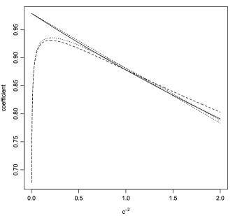
Figure 1: Model average coefficient on $\widehat{\beta}$ [evaluated as $\widehat{\beta}/\beta$], for normal likelihood with known error variance, $\sigma^{2}$. The plot here is for $n=10,\widehat{\beta}=1,\sigma^{2}=1$. The dashed line is for a uniform prior over models, and the solid line uses prior model probability $f(m_{1})\propto c^{-1}$. The dotted lines are approximations based on replacing $(2\pi)^{1/2}f_{1}(0|y)$ in (21) with its normal approximation $\exp(-\frac{i(\widehat{\beta})n}{2}\widehat{\beta}^{2})$, ignoring the dependence, to $O(n^{-1})$, of $f_{1}(0|y)$ on $c^{-2}$.

illustration of this is provided by Figure 1, where this coefficient is plotted for various values of $c^{-2}$, for the simple example of a normal distribution with known error variance, and prior odds $k=1$, corresponding to a uniform prior on model space. Note that a high value of the coefficient on $\widehat{\beta}$ corresponds to low shrinkage. It can be seen that, regardless of the value of $c^{-2}$, there is a certain amount of shrinkage toward the prior mean and the shrinkage is not a monotone function of $c^{-2}$. For values of $c^{-2}$ greater than 0.5, the shrinkage to the prior mean is an approximately linearly increasing function of $c^{-2}$ as expected. For small values of $c^{-2}$, posterior probability is increasingly concentrated on $m_{0}$ as $c^{-2}$ decreases (Lindley paradox) and hence the model-averaged estimate is increasingly shrunk to the prior mean. Adopting the approach advocated in this paper has the effect of setting $k\propto c^{-1}$ which mitigates this effect, and returns control over the shrinkage to the analyst.

6 Illustrated Examples

We illustrate our approach in a series of simulations and real data applications. For comparison, we also present results under other prior specifications, notably the hyper $g$-prior of Liang et al. (2008), for which computation is performed using the BAS package; see Clyde (2010).

Section 6.1 illustrates that unit information prior specifications (or other specifications suggestingsmaller prior parameter dispersion) can indeed significantly shrink posterior distributions toward zero. This effect suggests that although prior variances based on unit information might have desirable behavior with respect to model determination, they may unintentionally distort the parameter posterior distributions. We demonstrate that this can affect the predictive ability of routinely used model averaging approaches in which information is borrowed across a set of models.

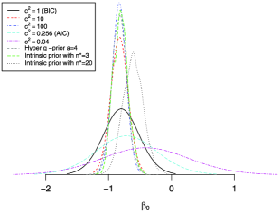
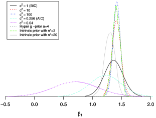
$\beta_{0}$	$\beta_{1}$

Figure 2: Posterior densities of parameters $\beta_{0}$ and $\beta_{1}$ under different prior dispersions; $c_{m}^{2}\!=\!c^{2}$ for all models $m$ for Example 6.1.

In Section 6.2 we illustrate the effect of Lindley’s paradox in a standard linear regression context emphasizing its dramatic effect on inference concerning model uncertainty. At the same time, we demonstrate that if instead of using the standard discrete uniform prior distribution for $f(m)$ we adopt our proposed adjusted prior distribution given by (11) with $p(m)=1$, the prior distribution for the model parameters can be made highly diffuse in a way which does not impact strongly on the posterior model probabilities.

Finally, Section 6.3 investigates the behavior of posterior model probabilities when substantive prior information about the parameters is available. We demonstrate through a real data example that the uniform prior on models may have a significant impact on posterior model probabilities and we illustrate the advantages of specifying prior model probabilities that are appropriately adjusted for parameter prior dispersions.

6.1 Example 1: A Simple Linear Regression Example

Montgomery, Peck and Vining (2001) investigated the effect of the logarithm of wind velocity ($x$), measured in miles per hour, on the production of electricity from a water mill ($y$), measured in volts, via a linear regression model of the form

$$y_{i}\sim N(\beta_{0}+\beta_{1}x_{i},\sigma^{2}),\quad i=1,\dots,n$$

based on $n=25$ data points. We calculate the posterior odds of the above model, denoted by $m_{1}$, against the constant model denoted by $m_{0}$, adopting the usual conjugate prior specification given by (3) with zero mean, variance $V_{m}=c_{m}^{2}n(\mathbf{X}_{m}^{T}\mathbf{X}_{m})^{-1}$ and $\alpha=\lambda=10^{-2}$. Since there is a high sample correlation coefficient of $0.978$ between $y$ and $x$, we expect that $m_{1}$ will be a posteriori strongly preferred to $m_{0}$. Indeed, the posterior probability of $m_{1}$ is very close to 1 for values of $c_{m}^{2}$ as large as $10^{28}$. This behavior provides a source of security with respect to the choice of $c_{m}^{2}$ and Lindley’s paradox, and we use this example to investigate the effect of $c_{m}^{2}$ on the posterior densities of $\beta_{0}$ and $\beta_{1}$; see Figure 2. We have used values of $c_{m}^{2}$ that represent highly diffuse priors with $c_{m}^{2}=10$ and $c_{m}^{2}=100$, the unit information prior that approximates BIC with $c_{m}^{2}=1$, a prior that approximates AIC for this sample size $c_{m}^{2}=(e^{2}-1)/n=0.256$ and a prior suggested by the risk inflation criterion (RIC) of Foster and George (1994) with $c_{m}^{2}=0.04$; see also George and Foster (2000). It is striking that the resulting posterior densities differ highly in both location and scale. The danger of misinformation when unit information priors are used was discussed in detail by Paciorek (2006).

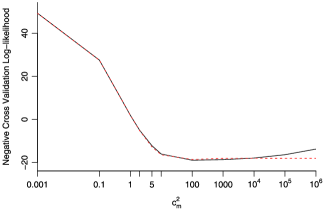
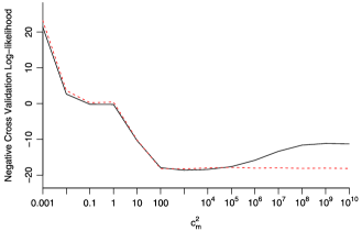
(a) g-prior $(V_{m}=c_{m}^{2}n(\mathbf{X}^{T}_{m}\mathbf{X}_{m})^{-1})$.	(b) Independence prior ($V_{m}=c_{m}^{2}\mathbf{I}_{d_{m}}$).

Figure 3: Negative cross-validation log-likelihood for two prior dispersion structures with uniform prior (solid line) and adjusted prior (dashed line) for Example 6.1.

We also investigated how the Zellner and Siow (1980) prior and the Liang et al. (2008) hyper $g$-prior behave in this example. With the recommended hyperparameter values $2<a\leq 4$, these priors produced posterior densities close to the low information $g$-prior with $c^{2}_{m}=100$; see Figure 2. The results are quite robust across this range for $a$ and, for example, quite large values of $a$, around 20, are required before the level of shrinkage becomes comparable to the unit information $g$-prior. Hence inferences arising from the hyper-$g$ prior are quite robust across the recommended range of hyperparameter values.

Finally, we examined the effect of intrinsic priors on posterior distributions for model parameters. We adopted the approach of Perez and Berger (2002) to construct an intrinsic (or expected posterior) prior by setting as a baseline prior the $g$-prior with $c^{2}=100$ and the null model as a reference. For this simple linear regression model the minimal training sample has size $n^{*}=3$. The resulting posterior distributions of $\beta_{0}$ and $\beta_{1}$, also shown in Figure 2, are in close agreement with the baseline $g$-prior. However, in variable selection problems the minimal training sample is usually set so that the full model can be estimated. Hence, the value of $n^{*}$ could be much higher if more covariates were available and this would affect the prior variance of the parameters. As an example, we have calculated the posterior densities of $\beta_{0}$ and $\beta_{1}$ when $n^{*}=20$, also displayed in Figure 2. The effect of the prior densities to the posterior distributions is dramatic. This nicely illustrates the effect of the training sample size in intrinsic priors; see the relevant discussion in Berger and Pericchi (2004).

We now investigate the effect of prior specification when prediction is of primary interest. A common way of evaluating predictive performance is to compute the negative cross-validation score (see Geisser and Eddy, 1979) given by

$$S=-\sum_{j=1}^{n}\log f^{p}(j),$$

where

$$f^{p}(j)=\sum_{m\in M}f(m)f(y_{j}|\mathbf{y}_{\setminus j},m)$$

is the model-averaged predictive density of observation $y_{j}$ given the rest of the data $\mathbf{y}_{\setminus j}$. Lower values of $S$ indicate greater predictive accuracy. Following Gelfand (1996) we estimate $f^{p}(j)$ from an MCMC sample by the inverse of the posterior (over $m,\bolds{\beta}_{m}$) mean of the inverse predictive density of observation $j$.

We generated three additional covariates that have correlation coefficients $0.99$, $0.97$ and $0.89$ with $x$ and performed the same model determination exercise. Posterior model probabilities for all models were calculated for all models under consideration. We used a $g$-prior with $V_{m}=c_{m}^{2}n(\mathbf{X}^{T}_{m}\mathbf{X}_{m})^{-1}$ and an independent prior with $V_{m}=c_{m}^{2}\mathbf{I}_{d_{m}}$. For the uniform prior on models combined with the unit information prior obtained by $c_{m}^{2}=1$, $S$ is far away from the minimum value achieved for higher values of $c_{m}^{2}$; see Figure 3(a). For $c_{m}^{2}>10^{5}$, $S$ increases due to the effect of Lindley’s paradox focusing posterior probability on models that are unrealistically simple. On the other hand, our proposed adjusted prior specification achieves the maximum predictive ability for any large value of $c_{m}^{2}$; see Figure 3(b). The same exercise was also repeated for the hyper-$g$ prior for various values of the hyperparameter $a$. The corresponding negative cross-validation score was close to the stabilized value of the $g$-prior and it was proven to be very robust for a wide range of values of $a$. Only for $a$ very close to $2$, did predictive ability start to deteriorate in a similar fashion to the $g$-prior.

This simulated data exercise does indicate that predictive ability can be optimized if highly dispersed prior parameter densities are chosen together with the adjusted prior over model space. Alternatively, in this example, the hyper-$g$ family is sufficiently robust to simultaneously provide a diffuse prior for model parameters, together with reasonable behavior under model uncertainty.

6.2 Example 2: Simulated Regressions

We now consider the first simulated dataset of Dellaportas, Forster and Ntzoufras (2002) based on $n=50$ observations of $15$ standardized independent normal covariates $X_{j},j=1,\ldots,15$, and a response variable $Y$ generated as

$$Y\sim N(X_{4}+X_{5},~{}2.5^{2}).$$ (22)

Assuming a conjugate normal inverse gamma prior distribution given by (3) with zero mean, $V_{m}=c_{m}^{2}\Sigma_{m}$ and $a=\lambda=10^{-2}$, we calculated posterior model probabilities for all models under consideration. Similar behavior is exhibited either when $\Sigma_{m}$ is specified as $\Sigma_{m}=n(\mathbf{X}_{m}^{T}\mathbf{X}_{m})^{-1}$ (described below) or as $\Sigma_{m}=\mathbf{I}_{d_{m}}$.

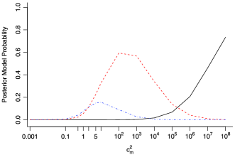
(a) Zellner’s $g$-prior with uniform prior on model space.

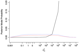
(b) Hyper-$g$ prior with uniform prior on model space.

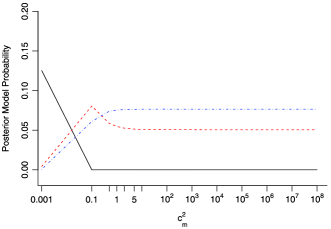
(c) Zellner’s $g$-prior with adjusted prior on model space.

Figure 4: Posterior model probabilities under different prior dispersions for the Dellaportas, Forster and Ntzoufras (2002) dataset of Section 6.2 generated using (22). Solid line: constant model; short dashed line: $1+X_{4}+X_{5}$ model; long dashed line: $1+X_{4}+X_{5}+X_{12}$ model.

Figure 4(a) and (b), illustrates the behavior of the posterior model probabilities, under a uniform prior on model space, of three indicative models. For the parameters we used the $g$-prior and the hyper-$g$ prior with $c_{m}^{2}=2n^{-1}/(a-2)$ obtained by equating the shrinkage proportion $g/(g-1)$ of the $g$-prior with its prior mean under the hyper-$g$ prior. The effect of Lindley’s paradox is more evident for the $g$-prior where all posterior probabilities are quite sensitive to the values of $c_{m}^{2}$ while the hyper-$g$ prior demonstrates a remarkable robustness for a wide range of prior parameter values and only for quite large values of $c_{m}^{2}$ which correspond to values of $a$ close to $2$ is Lindley’s paradox exhibited. We note that the hyper-$g$ prior seems to result in increased uncertainty on model space resulting in lower posterior model probabilities for the higher posterior probability models.

By contrast, using the adjusted prior in Figure 4(c) identifies $1+X_{4}+X_{5}+X_{12}$ as the highest probability model for any value of $c_{m}^{2}>1$. Note that, when $\Sigma_{m}=n(\mathbf{X}_{m}^{T}\mathbf{X}_{m})^{-1}$, $c_{m}^{2}=1$ represents the dispersion induced by the unit information prior. Similarly, Figure 5 summarizes the posterior inclusion probability of each variable $X_{j}$. Again, for the uniform prior these probabilities are sensitive to changes in $c_{m}^{2}$ across its range, whereas the adjusted prior produces stable results for $c_{m}^{2}>1$.

In a more detailed simulation study, we repeated the above analysis by generating $100$ datasets of the same model. The distribution of the posterior model probabilities over the $100$ simulated datasets reinforces the findings of the one-sample based simulation. We also repeated the above simulation experiment with a more challenging simulated dataset based on a simulation structure suggested by Nott and Kohn (2005). Each dataset consisted of $n=50$ observations and $p=15$ covariates and one response generated using the following sampling scheme:

$$\left\{\begin{array}[]{rcl}X_{j}&\sim&N(0,1)\quad\mbox{for }j=1,\ldots,10\\ X_{j}&\sim&N(0.3X_{1}+0.5X_{2}+0.7X_{3}\\ &&\hphantom{N(}{}+0.9X_{4}+1.1X_{5},1)\\ &&\mbox{for }j=11,\ldots,15\\ Y&\sim&N(4+2X_{1}-X_{5}+1.5X_{7}\\ &&\hphantom{N(}{}+X_{11}+0.5X_{13},2.5^{2})\end{array}\right\}.$$ (23)

The general conclusions of this study are in close agreement with the results obtained above. Further details are available in the electronic supplement which is available at http://stat-athens.aueb.gr/ ~jbn/papers/paper24.htm.

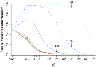
(a) Zellner’s $g$-prior with uniform prior on model space.

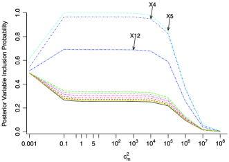
(b) Hyper-$g$ prior with uniform prior on model space.

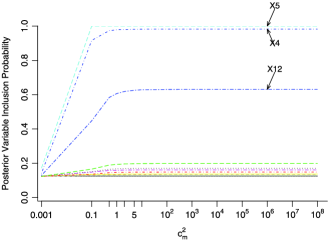
(c) Zellner’s $g$-prior with adjusted prior on model space.

Figure 5: Posterior variable inclusion probabilities under different prior dispersions for the Dellaportas, Forster and Ntzoufras (2002) dataset of Section 6.2 generated using (22).

6.3 Example 3: A $3\times 2\times 4$ Contingency Table Example with Available Prior Information

We consider data presented by Knuiman and Speed (1988) to illustrate how our proposed methodology performs in an example where prior information for the model parameters is available. The data consist of $491$ individuals classified in $n$ cells by categorical variables obesity (O: low, average, high), hypertension (H: yes, no) and alcohol consumption (A: 1, 1–2, 3–5, 6$+$ drinks per day). We adopt the notation of the full hierarchical log-linear model used by Dellaportas and Forster (1999):

$$y_{i}\sim\operatorname{Poisson}(\lambda_{i})\quad\mbox{for }i=1,2,\dots,n,\quad\log(\bolds{\lambda})=\mathbf{X}\bolds{\beta},$$

where $\bolds{\lambda}=(\lambda_{1},\dots,\lambda_{n})^{T}$, $\mathbf{X}$ is the $n\times n$ design matrix of the full model, $\bolds{\beta}=(\bolds{\beta}_{j};j\in{\mathcal{V}})$ is an $n\times 1$ parameter vector, $\bolds{\beta}_{j}$ are the model parameters that correspond to $j$ term and ${\mathcal{V}}$ is the set of all terms under consideration. All parameters here are defined using the sum-to-zero constraints. Dellaportas and Forster (1999) proposed as a default prior for parameters of log-linear models

$$\bolds{\beta}_{j}\sim N\pmatrix{\bolds{\mu}_{j},&k_{j}^{2}(\mathbf{X}_{j}^{T}\mathbf{X}_{j})^{-1}}$$ (24)

with $\bolds{\mu}_{j}$ being a vector of zeros and $k_{j}^{2}=2n$ for all $j\in{\mathcal{V}}=\{\varnothing,O,H,A,OH,OA,HA,OHA\}$; we denote this prior by DF.

In their analysis, Knuiman and Speed (1988) took into account some prior information available about the parameters $\bolds{\beta}_{j}$. In particular, prior to this study information was available indicating that $\bolds{\beta}_{OHA}$and $\bolds{\beta}_{OA}$ are negligible and only ${\mathcal{V}}=\{\varnothing,O,H,A,\allowbreak OH,HA\}$ should be considered. Moreover, theterm $\bolds{\beta}_{HA}$ is nonzero with a priori estimated effects $\overline{\bolds{\beta}}_{HA}^{T}=(0.204,-0.088,-0.271)$; note that the signs of the prior mean are opposite when compared with reported values of Knuiman and Speed since we have used a different ordering of the variable levels.

Knuiman and Speed adopted the prior (24) with $\bolds{\mu}_{HA}=\overline{\bolds{\beta}}_{HA}$ and $\bolds{\mu}_{j}={\bf 0}$ for $j\in{\mathcal{V}}\setminus\{HA\}$ and prior variance coefficients $k_{HA}^{2}=0.05$ and $k_{j}^{2}=\infty$ for $j\in\{\varnothing,O,H,A,OH\}$. In our data analysis we used $k_{j}^{2}=10^{4}$ instead of $k_{j}^{2}=\infty$. We denote this prior as KS. We also used a combination of the DF and KS priors, denoted by KS/DF, modifying slightly the KS prior so that $k_{j}^{2}=2n$ for terms $j\in\{\varnothing,O,H,A,OH\}$. Finally, an additional diffuse independence prior, denoted by IND, with zero prior mean and variance $10^{3}$ for all model parameters was also used.

In log-linear models $i(\bolds{\beta}_{m})$ depends on $\bolds{\beta}_{m}$ so to specify the adjusted prior we utilize the prior mean $\bolds{\mu}_{m}$ of $\bolds{\beta}_{m}$ resulting in

$$f(m)\propto p(m)|V_{m}|^{1/2}|\mathbf{X}_{m}^{T}\operatorname{Diag}(\bolds{\lambda}_{0})\mathbf{X}_{m}|^{1/2}n^{-d_{m}/2},$$

$$\quad\bolds{\lambda}_{0}=\exp(\mathbf{X}_{m}\bolds{\mu}_{m}),$$

while the prior parameters $p(m)$ were set equal to $\log p(m)=-\frac{d_{m}}{2}\log(2)$ in line with the DF prior.

Table 1: Prior and posterior model probabilities under different parameter and model prior densities for Example 6.3

	Parameter prior	Model space prior	Prior model probabilities				Posterior model probabilities
4-7,9-12			O${}\bolds{+}{}$H${}\bolds{+}{}$A	OH${}\bolds{+}{}$A	O${}\bolds{+}{}$HA	OH${}\bolds{+}{}$HA		O${}\bolds{+}{}$H${}\bolds{+}{}$A	OH${}\bolds{+}{}$A	O${}\bolds{+}{}$HA	OH${}\bolds{+}{}$HA
1.	DF	uniform	0.250	0.250	0.25$0\times^{1-5}$	0.25$0\times^{1-5}$		0.657	0.336	0.004	0.002
2.	KS	uniform	0.250	0.250	0.25$0\times^{1-5}$	0.25$0\times^{1-5}$		0.075	0.000	0.923	0.002
3.	KS/DF	uniform	0.250	0.250	0.25$0\times^{1-5}$	0.25$0\times^{1-5}$		0.059	0.023	0.638	0.280
4.	DF	adjusted	0.247	0.247	0.251$\times^{1-5}$	0.2557440.		0.677	0.317	0.004	0.002
5.	KS	adjusted	0.046	0.954	$2.0\times 10^{-6}$	$3.3\times 10^{-5}$		0.665	0.335	0.000	0.000
6.	KS/DF	adjusted	0.500	0.500	$1.7\times 10^{-5}$	$1.7\times 10^{-5}$		0.690	0.310	0.000	0.000
7.	IND	adjusted	0.003	0.996	$3.0\times 10^{-6}$	0.001$\times^{1-5}$		0.690	0.303	0.004	0.003

Posterior model probabilities (estimated using reversible jump MCMC) for all prior specifications are presented in Table 1. The top right panel of the table illustrates the striking effect of informative parameter priors on posterior model probabilities. The difficulty of making joint inferences on parameter and model space is evident by inspecting the sensitivity of model probabilities to different priors. However, the specification for adjusting the prior model probabilities has the effect that posterior model probabilities are robust under all prior specifications.

7 Conclusion

There are clearly alternative specifications for the prior model probabilities $p(m)$ which satisfy (11), and we do not seek to justify one over the other. Indeed, choosing model probabilities to satisfy (11) may not be appropriate in some situations. Hence, we do not propose (11) as a necessary condition for $f(m)$ although we do believe that there are compelling reasons for considering such a specification, perhaps as a default or reference position in the type of situations we have considered in this paper. What we do argue is that there is nothing sacred about a uniform prior distribution over models, and hence by implication, about the Bayes factor. It is completely reasonable to consider specifying $f(m)$ in a way which takes account of the prior distributions for the model parameters for individual models. Then, certainly within the contexts discussed in this paper, as demonstrated by the examples we have presented, the issues surrounding the role of the prior distribution for model parameters, in examples with model uncertainty, become much less significant.

References

- Bartlett (1957) {barticle}[mr] \bauthor\bsnmBartlett, \bfnmM. S.\binitsM. S. (\byear1957). \btitleComment on D. V. Lindley’s statistical paradox. \bjournalBiometrika \bvolume44 \bpages533–534. \bptnotecheck related\bptokimsref \endbibitem
- Berger and Pericchi (1996) {barticle}[mr] \bauthor\bsnmBerger, \bfnmJames O.\binitsJ. O. and \bauthor\bsnmPericchi, \bfnmLuis R.\binitsL. R. (\byear1996). \btitleThe intrinsic Bayes factor for model selection and prediction. \bjournalJ. Amer. Statist. Assoc. \bvolume91 \bpages109–122. \bidissn=0162-1459, mr=1394065 \bptokimsref \endbibitem
- Berger and Pericchi (2004) {barticle}[mr] \bauthor\bsnmBerger, \bfnmJames O.\binitsJ. O. and \bauthor\bsnmPericchi, \bfnmLuis R.\binitsL. R. (\byear2004). \btitleTraining samples in objective Bayesian model selection. \bjournalAnn. Statist. \bvolume32 \bpages841–869. \biddoi=10.1214/009053604000000238, issn=0090-5364, mr=2065191 \bptokimsref \endbibitem
- Chen, Ibrahim and Yiannoutsos (1999) {barticle}[mr] \bauthor\bsnmChen, \bfnmMing-Hui\binitsM.-H., \bauthor\bsnmIbrahim, \bfnmJoseph G.\binitsJ. G. and \bauthor\bsnmYiannoutsos, \bfnmConstantin\binitsC. (\byear1999). \btitlePrior elicitation, variable selection and Bayesian computation for logistic regression models. \bjournalJ. R. Stat. Soc. Ser. B Stat. Methodol. \bvolume61 \bpages223–242. \biddoi=10.1111/1467-9868.00173, issn=1369-7412, mr=1664057 \bptokimsref \endbibitem
- Chen et al. (2003) {barticle}[mr] \bauthor\bsnmChen, \bfnmMing-Hui\binitsM.-H., \bauthor\bsnmIbrahim, \bfnmJoseph G.\binitsJ. G., \bauthor\bsnmShao, \bfnmQi-Man\binitsQ.-M. and \bauthor\bsnmWeiss, \bfnmRobert E.\binitsR. E. (\byear2003). \btitlePrior elicitation for model selection and estimation in generalized linear mixed models. \bjournalJ. Statist. Plann. Inference \bvolume111 \bpages57–76. \biddoi=10.1016/S0378-3758(02)00285-9, issn=0378-3758, mr=1955872 \bptokimsref \endbibitem
- Chipman (1996) {barticle}[mr] \bauthor\bsnmChipman, \bfnmHugh\binitsH. (\byear1996). \btitleBayesian variable selection with related predictors. \bjournalCanad. J. Statist. \bvolume24 \bpages17–36. \biddoi=10.2307/3315687, issn=0319-5724, mr=1394738 \bptokimsref \endbibitem
- Chipman, George and McCulloch (2001) {bincollection}[mr] \bauthor\bsnmChipman, \bfnmHugh\binitsH., \bauthor\bsnmGeorge, \bfnmEdward I.\binitsE. I. and \bauthor\bsnmMcCulloch, \bfnmRobert E.\binitsR. E. (\byear2001). \btitleThe practical implementation of Bayesian model selection. In \bbooktitleModel Selection. \bseriesInstitute of Mathematical Statistics Lecture Notes—Monograph Series \bvolume38 \bpages65–134. \bpublisherIMS, \baddressBeachwood, OH. \biddoi=10.1214/lnms/1215540964, mr=2000752 \bptnotecheck related\bptokimsref \endbibitem
- Clyde (2000) {barticle}[auto:STB—2011/11/09—09:54:39] \bauthor\bsnmClyde, \bfnmM.\binitsM. (\byear2000). \btitleModel uncertainty and health effect studies for particulate matter. \bjournalEnvironmetrics \bvolume11 \bpages745–763. \bptokimsref \endbibitem
- Clyde (2010) {bmisc}[auto:STB—2011/11/09—09:54:39] \bauthor\bsnmClyde, \bfnmM.\binitsM. (\byear2010). \bhowpublishedThe BAS Package: Bayesian model averaging and stochastic search using Bayesian adaptive sampling (Version 0.91). Available at http://www.stat.duke.edu/ ~clyde/BAS/. \bptokimsref \endbibitem
- Cui and George (2008) {barticle}[mr] \bauthor\bsnmCui, \bfnmWen\binitsW. and \bauthor\bsnmGeorge, \bfnmEdward I.\binitsE. I. (\byear2008). \btitleEmpirical Bayes vs. fully Bayes variable selection. \bjournalJ. Statist. Plann. Inference \bvolume138 \bpages888–900. \biddoi=10.1016/j.jspi.2007.02.011, issn=0378-3758, mr=2416869 \bptokimsref \endbibitem
- Dawid (2011) {bincollection}[auto:STB—2011/11/09—09:54:39] \bauthor\bsnmDawid, \bfnmA. P.\binitsA. P. (\byear2011). \btitlePosterior model probabilities. In \bbooktitlePhilosophy of Statistics (\beditor\bfnmP. S.\binitsP. S. \bsnmBandyopadhyay and \beditor\bfnmM.\binitsM. \bsnmForster, eds.) \bpages607–630. \bpublisherElsevier, \baddressNew York. \bptokimsref \endbibitem
- Dellaportas and Forster (1999) {barticle}[mr] \bauthor\bsnmDellaportas, \bfnmPetros\binitsP. and \bauthor\bsnmForster, \bfnmJonathan J.\binitsJ. J. (\byear1999). \btitleMarkov chain Monte Carlo model determination for hierarchical and graphical log-linear models. \bjournalBiometrika \bvolume86 \bpages615–633. \biddoi=10.1093/biomet/86.3.615, issn=0006-3444, mr=1723782 \bptokimsref \endbibitem
- Dellaportas, Forster and Ntzoufras (2002) {barticle}[auto:STB—2011/11/09—09:54:39] \bauthor\bsnmDellaportas, \bfnmP.\binitsP., \bauthor\bsnmForster, \bfnmJ. J.\binitsJ. J. and \bauthor\bsnmNtzoufras, \bfnmI.\binitsI. (\byear2002). \btitleOn Bayesian model and variable selection using MCMC. \bjournalStat. Comput. \bvolume12 \bpages27–36. \bptokimsref \endbibitem
- Denison et al. (2002) {bbook}[mr] \bauthor\bsnmDenison, \bfnmDavid G. T.\binitsD. G. T., \bauthor\bsnmHolmes, \bfnmChristopher C.\binitsC. C., \bauthor\bsnmMallick, \bfnmBani K.\binitsB. K. and \bauthor\bsnmSmith, \bfnmAdrian F. M.\binitsA. F. M. (\byear2002). \btitleBayesian Methods for Nonlinear Classification and Regression. \bpublisherWiley, \baddressChichester. \bidmr=1962778 \bptokimsref \endbibitem
- Fernández, Ley and Steel (2001) {barticle}[mr] \bauthor\bsnmFernández, \bfnmCarmen\binitsC., \bauthor\bsnmLey, \bfnmEduardo\binitsE. and \bauthor\bsnmSteel, \bfnmMark F. J.\binitsM. F. J. (\byear2001). \btitleBenchmark priors for Bayesian model averaging. \bjournalJ. Econometrics \bvolume100 \bpages381–427. \biddoi=10.1016/S0304-4076(00)00076-2, issn=0304-4076, mr=1820410 \bptnotecheck year\bptokimsref \endbibitem
- Foster and George (1994) {barticle}[mr] \bauthor\bsnmFoster, \bfnmDean P.\binitsD. P. and \bauthor\bsnmGeorge, \bfnmEdward I.\binitsE. I. (\byear1994). \btitleThe risk inflation criterion for multiple regression. \bjournalAnn. Statist. \bvolume22 \bpages1947–1975. \biddoi=10.1214/aos/1176325766, issn=0090-5364, mr=1329177 \bptokimsref \endbibitem
- Geisser and Eddy (1979) {barticle}[mr] \bauthor\bsnmGeisser, \bfnmSeymour\binitsS. and \bauthor\bsnmEddy, \bfnmWilliam F.\binitsW. F. (\byear1979). \btitleA predictive approach to model selection. \bjournalJ. Amer. Statist. Assoc. \bvolume74 \bpages153–160. \bidissn=0003-1291, mr=0529531 \bptokimsref \endbibitem
- Gelfand (1996) {bincollection}[mr] \bauthor\bsnmGelfand, \bfnmAlan E.\binitsA. E. (\byear1996). \btitleModel determination using sampling-based methods. In \bbooktitleMarkov Chain Monte Carlo in Practice (\beditor\bfnmW. R.\binitsW. R. \bsnmGilks, \beditor\bfnmS.\binitsS. \bsnmRichardson and \beditor\bfnmD. J.\binitsD. J. \bsnmSpiegelhalter, eds.) \bpages145–161. \bpublisherChapman & Hall, \baddressLondon. \bidmr=1397969 \bptokimsref \endbibitem
- George and Foster (2000) {barticle}[mr] \bauthor\bsnmGeorge, \bfnmEdward I.\binitsE. I. and \bauthor\bsnmFoster, \bfnmDean P.\binitsD. P. (\byear2000). \btitleCalibration and empirical Bayes variable selection. \bjournalBiometrika \bvolume87 \bpages731–747. \biddoi=10.1093/biomet/87.4.731, issn=0006-3444, mr=1813972 \bptokimsref \endbibitem
- Ghosh (1994) {bbook}[auto:STB—2011/11/09—09:54:39] \bauthor\bsnmGhosh, \bfnmJ. K.\binitsJ. K. (\byear1994). \btitleHigher Order Asymptotics. \bpublisherIMS, \baddressHayward, CA. \bptokimsref \endbibitem
- Green (1995) {barticle}[mr] \bauthor\bsnmGreen, \bfnmPeter J.\binitsP. J. (\byear1995). \btitleReversible jump Markov chain Monte Carlo computation and Bayesian model determination. \bjournalBiometrika \bvolume82 \bpages711–732. \biddoi=10.1093/biomet/82.4.711, issn=0006-3444, mr=1380810 \bptokimsref \endbibitem
- Green (2003) {bincollection}[mr] \bauthor\bsnmGreen, \bfnmPeter J.\binitsP. J. (\byear2003). \btitleTrans-dimensional Markov chain Monte Carlo. In \bbooktitleHighly Structured Stochastic Systems. \bseriesOxford Statist. Sci. Ser. \bvolume27 \bpages179–206. \bpublisherOxford Univ. Press, \baddressOxford. \bidmr=2082410 \bptnotecheck related\bptokimsref \endbibitem
- Hans, Dobra and West (2007) {barticle}[mr] \bauthor\bsnmHans, \bfnmChris\binitsC., \bauthor\bsnmDobra, \bfnmAdrian\binitsA. and \bauthor\bsnmWest, \bfnmMike\binitsM. (\byear2007). \btitleShotgun stochastic search for “large ” regression. \bjournalJ. Amer. Statist. Assoc. \bvolume102 \bpages507–516. \biddoi=10.1198/016214507000000121, issn=0162-1459, mr=2370849 \bptokimsref \endbibitem
- Hoeting et al. (1999) {barticle}[mr] \bauthor\bsnmHoeting, \bfnmJennifer A.\binitsJ. A., \bauthor\bsnmMadigan, \bfnmDavid\binitsD., \bauthor\bsnmRaftery, \bfnmAdrian E.\binitsA. E. and \bauthor\bsnmVolinsky, \bfnmChris T.\binitsC. T. (\byear1999). \btitleBayesian model averaging: A tutorial. \bjournalStatist. Sci. \bvolume14 \bpages382–417. \biddoi=10.1214/ss/1009212519, issn=0883-4237, mr=1765176 \bptnotecheck related\bptokimsref \endbibitem
- Jeffreys (1961) {bbook}[mr] \bauthor\bsnmJeffreys, \bfnmHarold\binitsH. (\byear1961). \btitleTheory of Probability, \bedition3rd ed. \bpublisherClarendon Press, \baddressNew York. \bidmr=0187257 \bptokimsref \endbibitem
- Johnson (1970) {barticle}[mr] \bauthor\bsnmJohnson, \bfnmRichard A.\binitsR. A. (\byear1970). \btitleAsymptotic expansions associated with posterior distributions. \bjournalAnn. Math. Statist. \bvolume41 \bpages851–864. \bidissn=0003-4851, mr=0263198 \bptokimsref \endbibitem
- Kadane and Lazar (2004) {barticle}[mr] \bauthor\bsnmKadane, \bfnmJoseph B.\binitsJ. B. and \bauthor\bsnmLazar, \bfnmNicole A.\binitsN. A. (\byear2004). \btitleMethods and criteria for model selection. \bjournalJ. Amer. Statist. Assoc. \bvolume99 \bpages279–290. \biddoi=10.1198/016214504000000269, issn=0162-1459, mr=2061890 \bptokimsref \endbibitem
- Kass, Tierney and Kadane (1988) {bincollection}[mr] \bauthor\bsnmKass, \bfnmR. E.\binitsR. E., \bauthor\bsnmTierney, \bfnmL.\binitsL. and \bauthor\bsnmKadane, \bfnmJ. B.\binitsJ. B. (\byear1988). \btitleAsymptotics in Bayesian computation. In \bbooktitleBayesian Statistics, 3 (Valencia, 1987). \bseriesOxford Sci. Publ. \bpages261–278. \bpublisherOxford Univ. Press, \baddressNew York. \bidmr=1008051 \bptokimsref \endbibitem
- Kass and Wasserman (1995) {barticle}[mr] \bauthor\bsnmKass, \bfnmRobert E.\binitsR. E. and \bauthor\bsnmWasserman, \bfnmLarry\binitsL. (\byear1995). \btitleA reference Bayesian test for nested hypotheses and its relationship to the Schwarz criterion. \bjournalJ. Amer. Statist. Assoc. \bvolume90 \bpages928–934. \bidissn=0162-1459, mr=1354008 \bptokimsref \endbibitem
- Knuiman and Speed (1988) {barticle}[mr] \bauthor\bsnmKnuiman, \bfnmM. W.\binitsM. W. and \bauthor\bsnmSpeed, \bfnmT. P.\binitsT. P. (\byear1988). \btitleIncorporating prior information into the analysis of contingency tables. \bjournalBiometrics \bvolume44 \bpages1061–1071. \biddoi=10.2307/2531735, issn=0006-341X, mr=0981000 \bptokimsref \endbibitem
- Kohn, Smith and Chan (2001) {barticle}[mr] \bauthor\bsnmKohn, \bfnmRobert\binitsR., \bauthor\bsnmSmith, \bfnmMichael\binitsM. and \bauthor\bsnmChan, \bfnmDavid\binitsD. (\byear2001). \btitleNonparametric regression using linear combinations of basis functions. \bjournalStat. Comput. \bvolume11 \bpages313–322. \biddoi=10.1023/A:1011916902934, issn=0960-3174, mr=1863502 \bptokimsref \endbibitem
- Laud and Ibrahim (1995) {barticle}[mr] \bauthor\bsnmLaud, \bfnmPurushottam W.\binitsP. W. and \bauthor\bsnmIbrahim, \bfnmJoseph G.\binitsJ. G. (\byear1995). \btitlePredictive model selection. \bjournalJ. Roy. Statist. Soc. Ser. B \bvolume57 \bpages247–262. \bidissn=0035-9246, mr=1325389 \bptokimsref \endbibitem
- Laud and Ibrahim (1996) {barticle}[mr] \bauthor\bsnmLaud, \bfnmPurushottam W.\binitsP. W. and \bauthor\bsnmIbrahim, \bfnmJoseph G.\binitsJ. G. (\byear1996). \btitlePredictive specification of prior model probabilities in variable selection. \bjournalBiometrika \bvolume83 \bpages267–274. \biddoi=10.1093/biomet/83.2.267, issn=0006-3444, mr=1439783 \bptokimsref \endbibitem
- Ley and Steel (2009) {barticle}[mr] \bauthor\bsnmLey, \bfnmEduardo\binitsE. and \bauthor\bsnmSteel, \bfnmMark F. J.\binitsM. F. J. (\byear2009). \btitleOn the effect of prior assumptions in Bayesian model averaging with applications to growth regression. \bjournalJ. Appl. Econometrics \bvolume24 \bpages651–674. \biddoi=10.1002/jae.1057, issn=0883-7252, mr=2675199 \bptokimsref \endbibitem
- Liang et al. (2008) {barticle}[mr] \bauthor\bsnmLiang, \bfnmFeng\binitsF., \bauthor\bsnmPaulo, \bfnmRui\binitsR., \bauthor\bsnmMolina, \bfnmGerman\binitsG., \bauthor\bsnmClyde, \bfnmMerlise A.\binitsM. A. and \bauthor\bsnmBerger, \bfnmJim O.\binitsJ. O. (\byear2008). \btitleMixtures of priors for Bayesian variable selection. \bjournalJ. Amer. Statist. Assoc. \bvolume103 \bpages410–423. \biddoi=10.1198/016214507000001337, issn=0162-1459, mr=2420243 \bptokimsref \endbibitem
- Lindley (1957) {barticle}[mr] \bauthor\bsnmLindley, \bfnmD. V.\binitsD. V. (\byear1957). \btitleA statistical paradox. \bjournalBiometrika \bvolume44 \bpages187–192. \bptokimsref \endbibitem
- Madigan et al. (1995) {bmisc}[auto:STB—2011/11/09—09:54:39] \bauthor\bsnmMadigan, \bfnmD.\binitsD., \bauthor\bsnmRaftery, \bfnmA. E.\binitsA. E., \bauthor\bsnmYork, \bfnmJ.\binitsJ., \bauthor\bsnmBradshaw, \bfnmJ. M.\binitsJ. M. and \bauthor\bsnmAlmond, \bfnmR. G.\binitsR. G. (\byear1995). \bhowpublishedStrategies for graphical model selection. Selecting Models from Data: AI and Statistics IV (P. Cheesman and R. W. Oldford, eds.) 91–100. Springer, Berlin. \bptokimsref \endbibitem