Statistical Significance of the Netflix Challenge

Abstract

Inspired by the legacy of the Netflix contest, we provide an overview of what has been learned—from our own efforts, and those of others—concerning the problems of collaborative filtering and recommender systems. The data set consists of about 100 million movie ratings (from 1 to 5 stars) involving some 480 thousand users and some 18 thousand movies; the associated ratings matrix is about 99% sparse. The goal is to predict ratings that users will give to movies; systems which can do this accurately have significant commercial applications, particularly on the world wide web. We discuss, in some detail, approaches to “baseline” modeling, singular value decomposition (SVD), as well as kNN (nearest neighbor) and neural network models; temporal effects, cross-validation issues, ensemble methods and other considerations are discussed as well. We compare existing models in a search for new models, and also discuss the mission-critical issues of penalization and parameter shrinkage which arise when the dimensions of a parameter space reaches into the millions. Although much work on such problems has been carried out by the computer science and machine learning communities, our goal here is to address a statistical audience, and to provide a primarily statistical treatment of the lessons that have been learned from this remarkable set of data.

, and

1 Introduction and Summary

In what turned out to be an invaluable contribution to the research community, Netflix Inc. of Los Gatos, California, on October 2, 2006, publicly released a remarkable set of data, and offered a Grand Prize of one million US dollars to the person or team who could succeed in modeling this data to within a certain precisely defined predictive specification. While this contest attracted attention from many quarters—and most notably from within the computer science and artificial intelligence communities—the heart of this contest was a problem of statistical modeling, in a context known as collaborative filtering. Our goal in this paper is to provide a discussion and overview—from a primarily statistical viewpoint—of some of the lessons for statistics which emerged from this contest and its data set. This vantage will also allow us to search for alternative approaches for analyzing such data (while noting some open problems), as well as to attempt to understand the commonalities and interplay among the various methods that key contestants have proposed.

Netflix, the world’s largest internet-based movie rental company, maintains a data base of ratings their users have assigned (from 1 “star” to 5 “stars”) to movies they have seen. The intended use of this data is toward producing a system for recommending movies to users based on predicting how much someone is going to like or dislike any particular movie. Such predictions can be carried out using information on how much a user liked or disliked other movies they have rated, together with information on how much other users liked or disliked those same, as well as other, movies. Such recommender systems, when sufficiently accurate, have considerable commercial value, particularly in the context of the world wide web.

The precise specifications of the Netflix data are a bit involved, and we postpone our description of it to Section 2. Briefly, however, the training data consists of some 100 million ratings made by approximately 480,000 users, and involving some 18,000 movies. (The corresponding “matrix” of user-by-movie ratings is thus almost 99% sparse.) A subset of about 1.5 million ratings of the training set, called the probe subset, was identified. A further data set, called the qualifying data was also supplied; it was divided into two approximately equal halves, called the quiz and test subsets, each consisting of about 1.5 million cases, but with the ratings withheld. The probe, quiz and test sets were constructed to have similar statistical properties.

The Netflix contest was based on a root mean squared error (RMSE) criterion applied to the three million predictions required for the qualifying data. If one naively uses the overall average rating for each movie on the training data (with the probe subset removed) to make the predictions, then the RMSE attained is either 1.0104, 1.0528 or 1.0540, respectively, depending on whether it is evaluated in sample (i.e., on the training set), on the probe set or on the quiz set. Netflix’s own recommender system, called Cinematch, which is known to be based on computer-intensive but “straightforward linear statistical models with a lot of data conditioning” is known to attain (after fitting on the training data) an RMSE of either 0.9514 or 0.9525, on the quiz and test sets, respectively. (See Bennett and Lanning, 2007.) These values represent, approximately, a 9$\frac{1}{2}$% improvement over the naive movie-average predictor. The contest’s Grand Prize of one million US dollars was offered to anyone who could first improve the predictions so as to attain an RMSE value of not more than 90% of 0.9525, namely, 0.8572, or better, on the test set.

The Netflix contest began on Oct 2, 2006, and was to run until at least Oct 2, 2011, or until the Grand Prize was awarded. More than 50,000 contestants internationally participated in this contest. Yearly Progress Prizes of $50,000 US were offered for the best improvement of at least 1% over the previous year’s result. The Progress Prizes for 2007 and 2008 were won, respectively, by teams named “BellKor” and “BellKor in BigChaos.” Finally, on July 26, 2009, the Grand Prize winning entry was submitted by the “BellKor’s Pragmatic Chaos” team, attaining RMSE values of 0.8554 and 0.8567 on the quiz and test sets, respectively, with the latter value representing a 10.06% improvement over the contest’s baseline. Twenty minutes after that submission (and in accordance with the Last Call rules of the contest) a competing submission was made by “The Ensemble”—an amalgamation of many teams—who attained an RMSE value of 0.8553 on the quiz set, and an RMSE value of 0.8567 on the test set. To two additional decimal places, the RMSE values attained on the test set were 0.856704 by the winners, and 0.856714 by the runners up. Since the contest rules were based on test set RMSE, and also were limited to four decimal places, these two submissions were in fact a tie. It is therefore the order in which these submissions were received that determined the winner; following the rules, the prize went to the earlier submission. Fearing legal consequences, a second and related contest which Netflix had planned to hold was canceled when it was pointed out by a probabilistic argument (see Narayanan and Shmatikov, 2008) that, in spite of the precautions taken to preserve anonymity, it might theoretically be possible to identify some users on the basis of the seemingly limited information in the data.

Of course, nonrepeatability, and other vagaries of ratings by humans, itself imposes some lower bound on the accuracy that can be expected from any recommender system, regardless of how ingenious it may be. It now appears that the 10% improvement Netflix required to win the contest is close to the best that can be attained for this data. It seems fair to say that Netflix technical staff possessed “fortuitous insight” in setting the contest bar precisely where it did (i.e., 0.8572 RMSE); they also were well aware that this goal, even if attainable, would not be easy to achieve.

The Netflix contest has come and gone; in this story, significant contributions were made by Yehuda Koren and by “BellKor” (R. Bell, Y. Koren, C. Volinsky), “BigChaos” (M. Jahrer, A. Toscher), larger teams called “The Ensemble” and “Grand Prize,” “Gravity” (G. Takacs, I. Pilaszy, B. Nemeth,D. Tikk), “ML@UToronto” (G. Hinton, A. Mnih, R. Salakhutdinov; “ML” stands for “machine learning”), lone contestant Arkadiusz Paterek, “Pragmatic Theory” (M. Chabbert, M. Piotte) and many others. Noteworthy of the contest was the craftiness of some participants, and the open collaboration of others. Among such stories, one that stands out is that of Brandyn Webb, a “cybernetic epistemologist” having the alias Simon Funk (see Piatetsky, 2007). He was the first to publicly reveal use of the SVD model together with a simple algorithm for its implementation that allowed him to attain a good early score in the contest (0.8914 on the quiz set). He also maintains an engaging website at http:// sifter.org/~simon/journal.

Although inspired by it, our emphasis in this paper is not on the contest itself, but on the fundamentally different individual techniques which contribute to effective collaborative filtering systems and, in particular, on the statistical ideas which underpin them. Thus, in Section 2, we first provide a careful description of the Netflix data, as well as a number of graphical displays. In Section 3 we establish the notation we will use consistently throughout, and also include a table summarizing the performance of many of the methods discussed. Sections 4, 5, 6 and 7 then focus on four key “stand-alone” techniques applicable to the Netflix data. Specifically, in Section 4 we discuss ANOVA techniques which provide a baseline for most other methods. In Section 5 we discuss the singular value decomposition or SVD (also known as the latent factor model, or matrix factorization) which is arguably the most effective single procedure for collaborative filtering. A fundamentally different paradigm is based on neural networks—in particular, the restricted Boltzman machines (RBM)—which we describe in Section 6. Last of these stand-alone methods are the nearest neighbor or kNN methods which are the subject of Section 7.

Most of the methods that have been devised for collaborative filtering involve parameterizations of very high dimension. Furthermore, many of the models are based on subtle and substantive contextual insight. This leads us, in Section 8, to undertake a discussion of the issues involved in dimension reduction, specifically penalization and parametershrinkage. In Section 9 we digress briefly to describe certain temporal issues that arise, but we return to our main discussion in Section 10 where, after exploring their comparative properties, and taking stock of the lessons learned from the ANOVA, SVD, RBM and kNN models, we speculate on the requisite characteristics of effective models as we search for new model classes.

In response to the Netflix challenge, subtle, new and imaginative models were proposed by many contest participants. A selection of those ideas is summarized in Section 11. At the end, however, winning the actual contest proved not to be possible without the use of many hybrid models, and without combining the results from many prediction methods. This ensemble aspect of combining many procedures is discussed briefly in Section 11. Significant computational issues are involved in a data set of this magnitude; some numerical issues are described briefly in Section 13. Finally, in Section 14, we summarize some of the statistical lessons learned, and briefly note a few open problems. In large part because of the Netflix contest, the research literature on such problems is now sufficiently extensive that a complete listing is not feasible; however, we do include a broadly representative bibliography. For earlier background and reviews, see, for example, ACM SIGKDD (2007), Adomavicius and Tuzhilin (2005), Bell et al. (2009), Hill et al. (1995), Hoffman (2001b), Marlin (2004), Netflix (2006/2010), Park and Pennock (2007), Pu et al. (2008), Resnick and Varian (1997) and Tuzhilin at al. (2008).

2 The Netflix Data

In this section we provide a more detailed overview of the Netflix data; these in fact consist of two key components, namely, a training set and a qualifying set. The qualifying data set itself consists of two halves, called the quiz set and the test set; furthermore, a particular subset of the training set, called the probe set, was identified. The quiz, test and probe subsets were produced by a random three way split of a certain collection of data, and so were intended to have identical statistical properties.

The main component of the Netflix data—namely, the “training” set—can be thought of as a matrix of ratings consisting of 480,189 rows, corresponding to randomly selected anonymous users from Netflix’s customer base, and 17,770 columns, corresponding to movie titles. This matrix is 98.8% sparse; out of a possible $480{,}189\times 17{,}770=8{,}532{,}958{,}530$ entries, only 100,480,507 ratings are actually available. Each such rating is an integer value (a number of “stars”) between 1 (worst) and 5 (best). The data were collected between October 1998 and December 2005, and reflect the distribution of all ratings received by Netflix during that period. It is known that Netflix’s own database consisted of over 1.9 billion ratings, on over 85,000 movies, from over 11.7 million subscribers; see Bennett and Lanning (2007).

In addition to the training set, a qualifying data set consisting of 2,817,131 user–movie pairs was also provided, but with the ratings withheld. It consists of two halves: a quiz set, consisting of 1,408,342 user–movie pairs, and a test set, consisting of 1,408,789 pairs; these subsets were not identified. Contestants were required to submit predicted ratings for the entire qualifying set. To provide feedback to all participants, each time a contestant submitted a set of predictions Netflix made public the RMSE value they attained on a web-based Leaderboard, but only for the quiz subset. Prizes, however, were to be awarded on the basis of RMSE values attained on the test subset. The purpose of this was to prevent contestants from tuning their algorithms on the “answer oracle.”

Netflix also provided the dates on which each of the ratings in the data sets were made. The reason for this is that Netflix is more interested in predicting future ratings than in explaining those of the past. Consequently, the qualifying data set had been selected from among the most recent ratings that were made. However, to allow contestants to understand the sampling characteristics of the qualifying data set, Netflix identified the probe subset of 1,408,395 user-movie pairs within the training set (and hence with known ratings), whose distributional properties were meant to match those of the qualifying data set. (The quiz, test and probe subsets were produced from the random three-way split already mentioned.) As a final point, prior to releasing their data, Netflix applied some statistically neutral perturbations (such as deletions, changes of dates and/or ratings) to try to protect the confidentiality and proprietary nature of its client base.

In our discussions, the term “training set” will generally refer to the training data, but with the probe subset removed; this terminology is in line with common usage when a subset is held out during a statistical fitting process. Of course, for producing predictions to submit to Netflix, contestants would normally retrain their algorithms on the full training set (i.e., with probe subset included). As the subject of our paper is more concerned with collaborative filtering generally, rather than with the actual contest, we will make only limited reference to the qualifying data set, and mainly in our discussion on implicit data in Section 11, or when indicating certain scores that contestants achieved.

Finally, we mention that Netflix also provided the titles, as well as the release years, for all of the movies. In producing predictions for its internal use, Netflix’s Cinematch algorithm does make use of other data sources, such as (presumably) geographical, or other information about its customers, and this allows it to achieve substantial improvements in RMSE. However, it is known that Cinematch does not use names of the movies, or dates of ratings. In any case, to produce the RMSE values on which the contest was to be based, Cinematch was trained without any such other data. Nevertheless, no restrictions were placed on contestants from using external sources, as, for instance, other databases pertaining to movies. Interestingly however, none of the top contestants made use of any such auxiliary information.

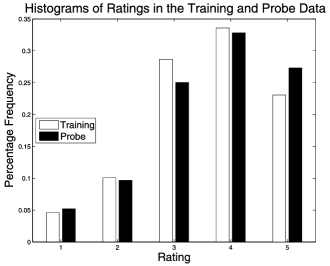
Figure 1: Frequency histograms for ratings in the training set (white) and probe set (black).

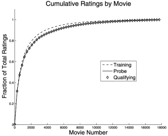
Figure 2: Cumulative proportion of ratings, by movies, for the training, probe and qualifying sets. Movies are on the horizontal axis, sorted from most to least rated.

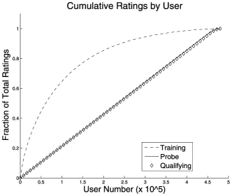
Figure 3: Cumulative proportion of ratings, by users, for the training, probe and qualifying sets. Users are on the horizontal axis, sorted by number of movies rated (from most to least).

Figures 1 through 6 provide some visualizations of the data. Figure 1 gives histograms for the ratings in the training set, and in the probe set. Reflecting temporal effects to be discussed in Section 9 (but see also Figure 5), the overall mean rating, 3.6736, of the probe set is significantly higher than the overall mean, 3.6033, of the training set. Figures 2 and 3 are plots (in lieu of histograms) of the cumulative number of ratings in the training, probe and qualifying sets. Figure 2 is cumulative by movies (horizontal axis, and sorted from most to least rated in the training set), while Figure 3 is cumulative by users. The steep rise in Figure 2 indicates, for instance, that the 100 and 1000 most rated movies account for over 14.3% and 62.5% of the ratings, respectively. In fact, the most rated movie (Miss Congeniality) was rated by almost half the users in the training set, while the least rated was rated only 3 times. Figure 2 also evidences a slight—although statistically significant—difference in the profiles for the training and the qualifying (and probe) data. In Figure 3, the considerable mismatch between the curve for the training data, with the curves for the probe and qualifying sets which match closely, reflects the fact that the representation of user viewership in the training set is markedly different from that of the cases for which predictions are required; clearly, Netflix constructed the qualifying data to have a much more uniform distribution of user viewership.

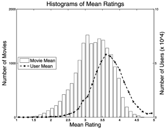
Figure 4: Histograms for mean movie ratings (bars) and mean user ratings (line with points) in the training set.

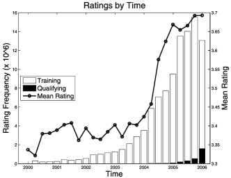
Figure 5: Temporal effects: Histograms for the dates (quarterly) of ratings in the training set (white bars) and qualifying set (inlaid black bars). The line with points shows quarterly mean ratings for the training data (scale on right).

Figure 4 provides histograms for the movie mean ratings and the user mean ratings. The reason for the evident mismatch between these two histograms is that the best rated movies were watched by disproportionately large numbers of users. Finally, Figure 5 exemplifies some noteworthy temporal effects in the data. Histograms are shown for the number of ratings, quarterly, in the training and in the qualifying data sets, with the dates in the qualifying set being much later than the dates in the training set. Figure 5 also shows a graph of the quarterly mean ratings for the training data (with the scale being at the right). Clearly, a significant rise in mean rating occurred starting around the beginning of 2004. Whether this occurred due to changes in the ratings definitions, to the introduction of a recommender system, to a change in customer profile, or due to some other reason, is not known.

Figure 6: Mean movie ratings versus (logarithm of) number of ratings (for a random subset of movies).

Finally, Figure 6 plots the mean movie ratings against the (log) number of ratings. (Only a random sample of movies is used so as not to clutter the plot.) The more rated movies do tend to have the higher mean ratings but with some notable exceptions, particularly among the less rated movies which can sometimes have very high mean ratings.

As a general comment, the layout of the Netflix data contains enormous variation. While the average number of ratings per user is 209, and the average number of ratings per movie is 5654.5 (over the entire training set), five users rated over 10,000 movies each, while many rated fewer than 5 movies. Likewise, while some movies were rated tens of thousands of times, most were rated fewer than 1000 times, and many less than 200 times. The extent of this variation implies large differences in the accuracies with which user and movie parameters can be estimated, a problem which is particularly severe for the users. Such extreme variation is among the features of typical collaborative filtering data which complicate their analyses.

3 Notation and a Summary Table

In this section we establish the notation we will adhere to in our discussions throughout this paper. We also include a table, which will be referred to in the sequel, of RMSE performance for many of the fitting methods we will discuss.

=15cm Predictive model RMSE Remarks and references $\hat{r}_{i,j}=\mu$ 1.1296 RMSE on probe set, using mean of training set $\hat{r}_{i,j}=\alpha_{i}$ 1.0688 Predict by user’s training mean, on probe set $\hat{r}_{i,j}=\beta_{j}$ 1.0528 Predict by movie’s training mean, on probe set $\hat{r}_{i,j}=\mu+\alpha_{i}+\beta_{j}$, naive 0.9945 Two-way ANOVA, no iteraction $\hat{r}_{i,j}=\mu+\alpha_{i}+\beta_{j}$ 0.9841 Two-way ANOVA, no iteraction “Global effects” 0.9657 Bell and Koren (2007a, 2007b, 2007c) Cinematch, on quiz set 0.9514 As reported by Netflix Cinematch, on test set 0.9525 Target is to beat this by 10% kNN 0.9174 Bell and Koren (2007a, 2007b, 2007c) “Global”${}+{}$SVD 0.9167 Bell and Koren (2007a, 2007b, 2007c) SVD 0.9167 Bell and Koren (2007a, 2007b, 2007c), on probe set “Global”${}+{}$SVD${}+{}$“joint kNN” 0.9071 Bell and Koren (2007a, 2007b, 2007c), on probe set “Global”${}+{}$SVD${}+{}$“joint kNN” 0.8982 Bell and Koren (2007a, 2007b, 2007c), on quiz set Simon Funk 0.8914 An early submission; Leaderboard TemporalDynamics${}+{}$SVD$++$ 0.8799 Koren (2009) Arkadiusz Paterek’s best score 0.8789 An ensemble of many methods; Leaderboard ML Team: RBM${}+{}$SVD 0.8787 See Section 6; Leaderboard Gravity’s best score 0.8743 November 2007; Leaderboard Progress Prize, 2007, quiz 0.8712 Bell, Koren and Volinsky (2007a, 2007b, 2007c) Progress Prize, 2007, test 0.8723 As above, but on the test set Progress Prize, 2008, quiz 0.8616 Bell, Koren and Volinsky (2008), Toscher and Jahrer (2008) Progress Prize, 2008, test 0.8627 As above, but on the test set Grand Prize, target 0.8572 10 % below Cinematch’s RMSE on test set Grand Prize, runner up 0.8553 The Ensemble, 20 minutes too late; on quiz set Grand Prize, runner up 0.8567 As above, but on the test set Grand Prize, winner 0.8554 BellKor${}+{}$BigChaos${}+{}$PragmaticTheory, on quiz set Grand Prize, winner 0.8567 As above, but on the test set []Selected RMSE values, compiled from various sources. Except as noted, RMSE values shown are either for the probe set after fitting on the training data with the probe set held out, or for the quiz set (typically from the Netflix Leaderboard) after fitting on the training data with the probe set included.

Table 1: RMSE values attained by various methods

Turning to notation, we will let $i=1,2,\ldots,I$ range over the users (or their indices) and $j=1,2,\ldots,J$ range over the movies (or their indices). For the Netflix training data, $I=480{,}189$ and $J=17{,}770$. Next, we will let $J(i)$ be the set of movies rated by user $i$ and $I(j)$ be the set of users who rated movie $j$. The cardinalities of these sets will be denoted variously as $J_{i}\equiv|J(i)|$ and $I_{j}\equiv|I(j)|$. We shall also use the notation $\mathcal{C}$ for the set of all user-movie pairs $(i,j)$ whose ratings are given. Denoting the total number of user-movie ratings in the training set by $N$, note that $N=|{\mathcal{C}}|=\sum_{i=1}^{I}J_{i}=\sum_{j=1}^{J}I_{j}$. The ratings are made on an ordered scale (such scales are known as “Likert scales”) and are coded as integers having values $k=1,2,\ldots,K$; for Netflix, $K=5$. The actual ratings themselves, for $(i,j)\in\mathcal{C}$, will be denoted by $r_{i,j}$. Averages of $r_{i,j}$ over $i\in I(j)$, over $j\in J(i)$, or over $\mathcal{C}$ (i.e., over movies, or users, or over the entire training data set) will be denoted by $r_{\bolds\cdot,j}$, $r_{i,\bolds\cdot}$ and $r_{\bolds\cdot,\bolds\cdot}$ respectively. Estimated values are denoted by “hats” as in $\hat{r}_{i,j}$, which may refer to the fitted value from a model when $(i,j)\in\mathcal{C}$, or to a predicted value otherwise. Many of the procedures we discuss are typically fitted to the residuals from a baseline fit such as an ANOVA; where this causes no confusion, we continue using the notations $r_{i,j}$ and $\hat{r}_{i,j}$ in referring to such residuals. Some procedures, however, involve both the original ratings as well as their residuals from other fits; in such cases, the residuals are denoted as $e_{i,j}$ and $\hat{e}_{i,j}$. Finally, the notation $I(j,j^{\prime})$ will refer to the set of all users who saw both movies $j$ and $j^{\prime}$, and $J(i,i^{\prime})$ will refer to the set of movies that were seen by both users $i$ and $i^{\prime}$.

Finally, we also include, in this section, a table which provides a summary, compiled from multiple sources, of the RMSE values attained by many of the methods discussed in this paper. The RMSE values shown in Table 1 are typically for the probe set, after fitting on the remainder of the training set; or where known, on the quiz set, after fitting on the entire training set; but exceptions to this are noted. References to the “Leaderboard” refer to performance on the quiz set publicly released by Neflix. We refer to Table 1 in our subsequent discussions.

4 ANOVA Baselines

ANOVA methods furnish baselines for many analyses. One basic approach—referred to as preprocessing—involves first removing global effects such as user and movie means, and using the residuals as input to subsequent models. Alternatively, such “row” and “column” effects can be incorporated directly into those models where they are sometimes referred to as biases. In any case, most models work best when global effects are explicitly accounted for. In this section we discuss minimizing the sum of squared errors criterion

$$\operatorname{\sum\sum}\limits_{(i,j)\in\mathcal{C}}(r_{i,j}-\hat{r}_{i,j})^{2}$$ (1)

using various ANOVA methods for the predictions $\hat{r}_{i,j}$ of the user-movie ratings $r_{i,j}$. Due to the large number of parameters, regularization (i.e., penalization) would normally be used, but we reserve our discussions of regularization issues to Section 8.

We first note that the best fitting model of the form

$$\hat{r}_{i,j}\equiv\mu\quad\mbox{ for all }i,j,$$ (2)

obtained by setting $\mu=$ 3.6033, the mean of all user-movie ratings in the training set (with probe removed), results in an RMSE on the training set equal to its standard deviation 1.0846; on the probe set, using this same $\mu$ results in an RMSE of 1.1296, although the actual mean and standard deviation for the probe set are 3.6736 and 1.1274.

Next, if we predict each rating by the mean rating for that user on the training set, thus fitting the model

$$\hat{r}_{i,j}=\mu+\alpha_{i},$$ (3)

we obtain an RMSE of 0.9923 on the training set, and 1.0688 using the same values on the probe. If, instead, we predict each rating by the mean for that movie, thus fitting

$$\hat{r}_{i,j}=\mu+\beta_{j},$$ (4)

we obtain RMSE values 1.0104 and 1.0528 on the training and probe sets, respectively. The solutions for (2)–(4) are just the least squares fits associated with

$$\operatorname{\sum\sum}\limits_{(i,j)\in\mathcal{C}}(r_{i,j}-\mu)^{2},$$

$$\operatorname{\sum\sum}\limits_{(i,j)\in\mathcal{C}}(r_{i,j}-\mu-\alpha_{i})^{2}\quad\mbox{and}$$ (5)

$$\operatorname{\sum\sum}\limits_{(i,j)\in\mathcal{C}}(r_{i,j}-\mu-\beta_{j})^{2},$$

respectively, where $\mathcal{C}$ is the set of indices $(i,j)$ over the training set. Histograms of the user and movie means were given in Figure 4; we note, for later use, that the the variances of the user and movie means on the test set (with probe removed) are 0.23074 and 0.27630, corresponding to standard deviations of 0.48035 and 0.52564, respectively.

We now consider two-factor models of the form

$$\hat{r}_{i,j}=\mu+\alpha_{i}+\beta_{j}.$$ (6)

Identifiability conditions, such as $\sum_{i}\alpha_{i}=0$ and$\sum_{j}\beta_{j}=0$, would normally be imposed, although they become unnecessary under typical regularization. If we were to proceed as in a balanced two-way layout (i.e., with no ratings missing), then we would first estimate $\mu$ as the mean of all available ratings; the values of $\alpha_{i}$ and $\beta_{j}$ would then be estimated as the row and column means, over the available ratings, after $\mu$ has been subtracted throughout. Doing this results in RMSE values of 0.9244 and 0.9945 on the training and probe sets. If we proceed sequentially, the order of the operations for estimating the $\alpha_{i}$’s and the $\beta_{j}$’s will matter: If we estimate the $\alpha_{i}$’s first and subtract their effects before estimating the $\beta_{j}$’s, the result will not be the same as first estimating the $\beta_{j}$’s and subtracting their effect before estimating the $\alpha_{i}$’s; these procedures result, respectively, in RMSE values of 0.9218 and 0.9177 on the training set.

The layout for the Netflix data is unbalanced, with the vast majority of user-movie pairings not rated; we therefore seek to minimize

$$\sum_{(i,j)\in\mathcal{C}}(r_{i,j}-\mu-\alpha_{i}-\beta_{j})^{2}$$ (7)

over the training set. This quadratic criterion is convex, however, standard methods for solving the “normal” equations, obtained by setting derivatives with respect to $\mu$, $\alpha_{i}$ and $\beta_{j}$ to zero, involve matrix inversions which are not feasible over such high dimensions. The optimization of (7) may, however, be carried out using either an EM or a gradient descent algorithm. When no penalization is imposed, minimizing (7) results in an RMSE value of 0.9161 on the training set, and 0.9841 on the probe subset.

A consideration when fitting (6) as well as other models is that some predicted ratings $\hat{r}_{i,j}$ can fall outside the $[1,5]$ range. This can occur when highly rated movies are rated by users prone to giving high ratings, or when poorly rated movies are rated by users prone to giving low ratings. Under optimization of (7) over the test set, approximately 5.1 million $\hat{r}_{i,j}$ estimates fall below 1, and 19.4 million fall above 5. Although we may Winsorize (clip) these $\hat{r}_{i,j}$ to lie in $[1,5]$, clipping in advance need not be optimal when residuals from a baseline fit are input to other procedures. We do not consider here the problem of minimizing (7) when $\mu+\alpha_{i}+\beta_{j}$ there is replaced by a Winsorized version.

Of course, not all is well here. The differences in RMSE values between the training and the probe sets reflect temporal effects, some of which were already noted. Furthermore, these models have parameterizations of high-dimensions and have therefore been overfit, resulting in inferior predictions. These issues will be dealt with in Sections 8 and 9.

Finally, we remark that interaction terms can be added to (6). The standard approach $\hat{r}_{i,j}=\mu+\alpha_{i}+\beta_{j}+\gamma_{i,j}$ will not be effective, although it could possibly be combined with regularization. Alternatively, interactions could be based on user $\times$ movie groupings via “many to one” functions $a(i)$ and $b(j)$, and models such as

$$\hat{r}_{i,j}=\mu+\alpha_{i}+\beta_{j}+\gamma_{a(i),b(j)}.$$ (8)

There are many possibilities for defining such groups; for example, the covariates discussed in Section 11 or nearest neighbor methods (kNN) can be used to construct suitable $a(i)$ and $b(j)$. Some further interaction-type ANOVA models are considered in Section 10.

5 SVD Methods

In statistics, the singular value decomposition(SVD) is best known for its connection to principal components: If $X=(X_{1},X_{2},\ldots,X_{n})^{\prime}$ is a random vector of means $0$, and $n\times n$ covariance matrix $\Sigma$, then one may represent $\Sigma$ as a linear combination of mutually orthogonal rank 1 matrices, as in

$$\Sigma=\sum_{j=1}^{n}\lambda_{j}P_{j}P_{j}^{\prime},$$

where $\lambda_{1}\geq\lambda_{2}\geq\cdots\geq\lambda_{n}\geq 0$ are ordered eigenvalues of $\Sigma$, and $P_{j}$ corresponding orthonormal (column) eigenvectors. The principal components are the random variables $P_{j}^{\prime}X$. Less commonly known is that the $n\times n$ matrix ${\mathcal{T}}^{(k)}=\sum_{j=1}^{k}\lambda_{j}P_{j}P_{j}^{\prime}$ gives the best rank $k$ reconstruction of $\Sigma$, in the sense of minimizing the Frobenius norm $\|\Sigma-{\mathcal{T}}^{(k)}\|$, defined as the square root of the sum of the squares of its entries.

These results generalize. If $A$ is an arbitrary real-valued $m\times n$ matrix, its singular value decomposition is given by

$$A=UDV^{\prime},$$

where $U\,{=}\,(U_{1},U_{2},\ldots,U_{m})$ is an $m\times m$ matrix whose columns $U_{j}$ are orthonormal eigenvectors of $AA^{\prime}$, where $V=(V_{1},V_{2},\ldots,V_{n})$ is an $n\times n$ matrix whose columns $V_{j}$ are orthonormal eigenvectors of $A^{\prime}A$, and where $D$ is an $m\times n$ “diagonal” matrix whose diagonal entries may be taken as the descending order nonnegative values

$$\lambda_{j} = +\sqrt{\{\operatorname{eigval}AA^{\prime}\}_{j}}$$

$$= +\sqrt{\{\operatorname{eigval}A^{\prime}A\}_{j}},\quad j=1,2,\ldots,\min(m,n),$$

called the singular values of $A$. The columns of $V$ and $U$ provide natural bases for inputs to and outputs from the linear transformation $A$. In particular, $AV_{j}=\lambda_{j}U_{j}$, $A^{\prime}U_{j}=\lambda_{j}V_{j}$, so given an input $B=\sum_{j=1}^{n}c_{j}V_{j}$, the corresponding output is $AB=\sum_{j=1}^{{\rm min}(m,n)}\lambda_{j}c_{j}U_{j}$.

Given an SVD of $A$, the Eckart–Young Theorem states that, for a given $k<\min(m,n)$, the best rank $k$ reconstruction of $A$, in the sense of minimizing the Frobenius norm of the difference, is $U^{(k)}D^{(k)}(V^{(k)})^{\prime}$, where $U^{(k)}$ is the $m\times k$ matrix formed from the first $k$ columns of $U$, $V^{(k)}$ is the $n\times k$ matrix formed by the first $k$ columns of $V$, and $D^{(k)}$ is the upper left $k\times k$ block of $D$. This reconstruction may be expressed in the form $FG^{\prime}$ where $F$ is $m\times k$ and $G$ is $k\times n$; the reconstruction is thus formed from the inner products between the $k$-vectors comprising $F$ with those comprising $G$. These $k$-vectors may be thought of as associated, respectively, with the rows and the columns of $A$, and (in applications) the components of these vectors are often referred to as features. A numerical consequence of the Eckart–Young Theorem is that “best” rank $k$ approximations can be determined iteratively: given a best rank $k-1$ approximation, $FG^{\prime}$, say, a best rank $k$ approximation is obtained by attaching a column vector to each of $F$ and $G$ which provide a best fit to the residual matrix $A-FG^{\prime}$. SVD algorithms can therefore be quite straightforward. Here, however, we are specifically concerned with algorithms applicable to matrices which are sparse. We briefly discuss two such algorithms, useful in collaborative filtering, namely, alternating least squares (ALS) and gradient descent. Some relevant references are Bell and Koren (2007c), Bell, Koren and Volinsky (2007a), Funk (2006/2007), Koren, Bell and Volinsky (2009), Raiko, Ilin and Karhunen (2007), Srebro and Jaakkola (2003), Srebro, Rennie and Jaakkola (2005), Takacs et al. (2007, 2008a, 2008b, 2008c), Wu (2007) and Zhou et al. (2008). See also Hofmann (2001a, 2004), Hofmann and Puzicha (1999), Kim and Yum (2005), Marlin and Zemel (2004), Rennie and Srebro (2005), Sali (2008) and Zou et al. (2006).

The alternating least squares (ALS) method for determining the best rank $p$ reconstruction involves expressing the summation in the objective function in two ways:

$$\sum\sum_{\mathcal{C}}\Biggl{(}r_{i,j}-\sum_{k=1}^{p}u_{i,k}v_{j,k}\Biggr{)}^{2}$$

$$\quad=\sum_{j=1}^{J}\sum_{i\in I(j)}\Biggl{(}r_{i,j}-\sum_{k=1}^{p}u_{i,k}v_{j,k}\Biggr{)}^{2}$$ (9)

$$\quad=\sum_{i=1}^{I}\sum_{j\in J(i)}\Biggl{(}r_{i,j}-\sum_{k=1}^{p}u_{i,k}v_{j,k}\Biggr{)}^{2}.$$

The $u_{i,k}$ may be initialized using small independent normal variables, say. Then, for each fixed $j$, we carry out the least squares fit for the $v_{j,k}$ based on the inner sum in the middle expression of (5). And then, for each fixed $i$, we carry out the least squares fit for $u_{i,k}$ based on the inner sum of the last expressions in (5). This procedure is iterated until convergence; several dozen iterations typically suffice.

ALS for SVD with regularization proceeds similarly. For example, minimizing

$$\sum\sum_{\mathcal{C}}\Biggl{(}r_{i,j}-\sum_{k=1}^{p}u_{i,k}v_{j,k}\Biggr{)}^{2}$$

(10)

$${}+\lambda_{1}\sum_{i=1}^{I}\|u_{i}\|^{2}+\lambda_{2}\sum_{j=1}^{J}\|v_{j}\|^{2}$$

leads to iterations which alternate between minimizing

$$\sum_{i\in I(j)}\Biggl{(}r_{i,j}-\sum_{k=1}^{p}u_{i,k}v_{j,k}\Biggr{)}^{2}+\lambda_{1}\|v_{j}\|^{2}$$ (11)

with respect to the $v_{j,k}$, and then minimizing

$$\sum_{j\in J(i)}\Biggl{(}r_{i,j}-\sum_{k=1}^{p}u_{i,k}v_{j,k}\Biggr{)}^{2}+\lambda_{2}\|u_{i}\|^{2}$$ (12)

with respect to the $u_{i,k}$; these are just ridge regression problems.

ALS can also be performed one feature at a time, with the advantage of yielding factors in descending order of importance. To do this, we initialize as before, and again arrange the order of summation in the objective function in two different ways; for the first feature, this is

$$\sum_{j=1}^{J}\biggl{[}\sum_{i\in I(j)}(r_{i,j}-u_{i,1}v_{j,1})^{2}\biggr{]}$$

(13)

$$\quad=\sum_{i=1}^{I}\biggl{[}\sum_{j\in J(i)}(r_{i,j}-u_{i,1}v_{j,1})^{2}\biggr{]}.$$

We then iterate between the least squares problems of the inner sums in (5), namely,

$$\hat{v}_{j,1}=\sum_{i\in I(j)}u_{i,1}r_{i,j}\Big{/}\sum_{i\in I(j)}u_{i,1}^{2}$$ (14)

for all $j$, and then

$$\hat{u}_{i,1}=\sum_{j\in J(i)}v_{j,1}r_{i,j}\Big{/}\sum_{j\in J(i)}v_{j,1}^{2}$$ (15)

for all $i$, until convergence. After $k-1$ features have been fit, we compute the residuals

$$e_{i,j}=r_{i,j}-\sum_{\ell=1}^{k-1}u_{i,\ell}v_{j,\ell}$$

and replace (14) and (15) by

$$\hat{v}_{j,k}=\sum_{i\in I(j)}u_{i,k}e_{i,j}\Big{/}\sum_{i\in I(j)}u_{i,k}^{2}$$

and

$$\hat{u}_{i,k}=\sum_{j\in J(i)}v_{j,k}e_{i,j}\Big{/}\sum_{j\in J(i)}v_{j,k}^{2},$$

ranging over all $j$ and all $i$, respectively.

Regularization in one-feature-at-a-time ALS can be effected in several ways. Bell, Koren and Volinsky (2007a) shrink the residuals $e_{i,j}$ via

$$e_{i,j}\leftarrow\frac{n_{i,j}}{n_{i,j}+\lambda_{k}}e_{i,j},$$

where $n_{i,j}=\min(I_{j},J_{i})$ measures the “support”for $r_{i,j}$, and they increase the shrinkage parameter $\lambda_{k}$ with each feature $k$. Alternately, one could add a regularization term

$$\lambda_{k}(\|u_{k}\|^{2}+\|v_{k}\|^{2})$$

when fitting the $k$th feature, choosing the $\lambda_{k}$ by cross-validation.

Finally, we consider gradient descent approaches for fitting SVD models. For an SVD of dimension $p$, say, we first initialize all $u_{i,k}$ and $v_{j,k}$ in

$$\sum\sum_{\mathcal{C}}\Biggl{(}r_{i,j}-\sum_{k=1}^{p}u_{i,k}v_{j,k}\Biggr{)}^{2}.$$

Then write

$$e_{i,j}=r_{i,j}-\sum_{k=1}^{p}u_{i,k}v_{j,k},$$

and note that

$$\frac{\partial e_{i,j}^{2}}{\partial u_{i,k}}=-2e_{i,j}v_{j,k}$$

and

$$\frac{\partial e_{i,j}^{2}}{\partial v_{j,k}}=-2e_{i,j}u_{i,k}.$$

Updating can then be done locally following the negative gradients:

$$u_{i,k}^{\mathrm{new}} = u_{i,k}^{\mathrm{old}}+2\eta e_{i,j}v_{j,k}^{\mathrm{old}}\quad\mbox{and}$$

$$v_{j,k}^{\mathrm{new}} = v_{j,k}^{\mathrm{old}}+2\eta e_{i,j}u_{i,k}^{\mathrm{old}},$$

where the learning rate $\eta$ controls for overshoot. For a given $(i,j)\in\mathcal{C}$, these equations are used to update the $u_{i,k}$ and $v_{j,k}$ for all $k$; we then cycle over the $(i,j)\in\mathcal{C}$ until convergence. If we regularize the problem, as in

$$\sum\sum_{\mathcal{C}}\Biggl{(}r_{i,j}-\sum_{k=1}^{p}u_{i,k}v_{j,k}\Biggr{)}^{2}$$

(17)

$$\quad{}+\lambda\biggl{(}\sum_{i}\|u_{i}\|^{2}+\sum_{j}\|v_{j}\|^{2}\biggr{)},$$

the update equations become

$$\hskip 6.0pt\qquad u_{i,k}^{\mathrm{new}} = u_{i,k}^{\mathrm{old}}+\eta\biggl{(}2e_{i,j}v_{j,k}^{\mathrm{old}}-\frac{\lambda}{J_{i}}u_{i,k}^{\mathrm{old}}\biggr{)}\quad\mbox{and}$$

$$v_{j,k}^{\mathrm{new}} = v_{j,k}^{\mathrm{old}}+\eta\biggl{(}2e_{i,j}u_{i,k}^{\mathrm{old}}-\frac{\lambda}{I_{j}}v_{j,k}^{\mathrm{old}}\biggr{)}.$$

We note that, as in ALS, there are other ways to sequence the updating steps in gradient descent. Simon Funk (2006/2007), for instance, trained the features one at a time. To train the $k$th feature, one initializes the $u_{i,k}$ and $v_{j,k}$ randomly, and then loops over all $(i,j)\in{\mathcal{C}}$, updating the $k$th feature for all users and all movies. The updating equations are as before [e.g., (5)] except based on residuals $e_{i,j}=r_{i,j}-\sum_{\ell=1}^{k}u_{i,\ell}v_{j,\ell}$. After convergence, one proceeds to the next feature.

We remark that sparse SVD problems are known to be nonconvex and to have multiple local minima; see, for example, Srebro and Jaakkola (2003). Nevertheless, starting from different initial conditions, we found that SVD seldom settled into entirely unsatisfactory minima, although the minima attained did vary slightly. The magnitude of these differences was commensurate with the variation inherent among the options available for regularization. We also found that averaging the results from several SVD fits started at different initial conditions could lead to better results than a single SVD fit of a higher dimension. On this point, see also Wu (2007). Finally, we note the recent surge of work on a problem referred to as matrix completion; see, for example, Candes and Plan (2009).

6 Neural Networks and RBMs

A restricted Boltzman machine (RBM) is a neural network consisting of one layer of visible units, and one layer of invisible ones; there are no connections between units within either of these layers, but all units of one layer are connected to all units of the other layer. To be an RBM, these connections must be bidirectional and symmetric; some definitions require that the units only take on binary values, but this restriction is unnecessary. We remark that the symmetry condition is only needed so as to simplify the training process. See Figure 7; additional clarification will emerge from the discussion below. The name for these networks derives from the fact that their governing probability distributions are analogous to the Boltzman distributions which arise in statistical mechanics. For further background, see, for example, Hertz, Krogh and Palmer (1991), Section 7.1, Izenman (2008), Chapter 10, or Ripley (1996), Section 8.4. See also Bishop (1995, 2006). We will describe the RBM model that has been applied to the Netflix data by Salakhutdinov, Mnih and Hinton (2007), whom we will also refer to as SMH.

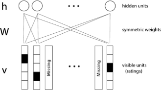
Figure 7: The RBM model for a single user: Each of the user’s hidden units is connected to every visible unit (a multinomial observation) that represents a rating made by that user. Every user is associated with one RBM, and the RBM models for the different users are linked through the common symmetric weight parameters $W_{j,f}^{k}$.

In the SMH model, to each user $i$, there corresponds a length $F$ vector of hidden (i.e., unobserved) units, or features, $h=(h_{1},h_{2},\ldots,h_{F})$. These features, $h_{f}$, for $f=1,2,\ldots,F$, are random variables posited to take on binary values, 0 or 1. Note that subscripting to indicate the dependence of $h$ on the $i$th user has been suppressed. Next, instead of thinking of the ratings of the $i$th user as the collection of values $r_{i,j}$ for $j\in J(i)$, we think of this user’s ratings as the collection of vectors $v_{j}=(v_{j}^{1},v_{j}^{2},\ldots,v_{j}^{K})$, for $j\in J(i)$, that is, for each of the movies he or she has seen. Each of these vectors is defined by setting all of its elements to 0, except for one: namely, $v_{j}^{k}=1$, corresponding to $r_{i,j}=k$. Here $K$ is the number of possible ratings; for Netflix, $K=5$. The collection of these $v_{j}$ vectors for our $i$th user [with $j\in J(i)$] will be denoted by $v$. Here again, the dependence of $v$, as well as of the $v_{j}$ and the $v_{j}^{k}$, on the user $i$ is suppressed.

We next introduce the symmetric weight parameters $W_{j,f}^{k}$ for $1\leq j\leq J$, $1\leq f\leq F$ and $1\leq k\leq K$, which link each of the $F$ hidden features of a user with each of the $J$ possible movies; these weights also carry a dependence on the rating values $k$.The $W_{j,f}^{k}$ are not dependent on the user; the same weights apply to all users, however, only weights for the movies he or she has rated will be relevant for any particular user.

We next specify the underlying stochastic model. First, the distributions of the $(v,h)$ are assumed to be independent across users. We therefore only need to specify a probability distribution on the collection $(v,h)$ for the $i$th user. This distribution is determined by its two conditional distributions modeled as follows: The conditional distribution of the $i$th user’s observed ratings information $v$, given that user’s hidden features vector $h$, is modeled as a (one-trial) multinomial distribution

$$P(v_{j}^{k}=1|h)$$

(19)

$$\quad=\frac{\exp(b_{j}^{k}+\sum_{f=1}^{F}h_{f}W_{j,f}^{k})}{\sum_{\ell=1}^{K}\exp(b_{j}^{\ell}+\sum_{f=1}^{F}h_{f}W_{j,f}^{\ell})},$$

where the denominator is just a normalizing factor. Next, the conditional distributions of the $i$th user’s hidden features variables, given that user’s observed ratings $v$, are modeled as conditionally independent Bernoulli variables

$$\qquad P(h_{f}=1|v)=\sigma\Biggl{(}b_{f}+\sum_{j\in J(i)}\sum_{k=1}^{K}v_{j}^{k}W_{j,f}^{k}\Biggr{)},$$ (20)

where $\sigma(x)=1/(1+e^{-x})$ is the sigmoidal function. Note that (20) is equivalent to the linear logit model

$$\log\biggl{(}\frac{P(h_{f}=1|v)}{1-P(h_{f}=1|v)}\biggr{)}$$

(21)

$$\quad=b_{f}+\sum_{j\in J(i)}\sum_{k=1}^{K}v_{j}^{k}W_{j,f}^{k};$$

in effect, (20)/(6) models user features in terms of the movies the user has rated, and the user’s ratings for them. Note that the weights (interaction parameters) $W_{j,f}^{k}$ are assumed to act symmetrically in (6) and (20). The parameters $b_{j}^{k}$ and $b_{f}$ are referred to as biases; the $b_{j}^{k}$ may be initialized to the logs of their respective sample proportions over all users. We remark that in this model there is no analogue for user biases.

To obtain the joint density of $v$ and $h$ from their two conditional distributions, we make use of the following result: Suppose $f(x,y)$ is a joint density for $(X,Y)$, and that $f_{1}(x|y)$, $f_{2}(y|x)$ are the corresponding conditional density functions for $X|Y$ and $Y|X$. Then noting the elementary equalities

$$f(x,y) = f_{1}(x|y)\times\frac{f_{2}(y|x^{*})}{f_{1}(x^{*}|y)}\times f_{X}(x^{*})$$

$$= f_{2}(y|x)\times\frac{f_{1}(x|y^{*})}{f_{2}(y^{*}|x)}\times f_{Y}(y^{*}),$$

we see that $f(x,y)$ can be determined from $f_{1}$ and $f_{2}$ since it is proportional to either of

$$f_{1}(x|y)\times\frac{f_{2}(y|x^{*})}{f_{1}(x^{*}|y)}\quad\mbox{and}\quad f_{2}(y|x)\times\frac{f_{1}(x|y^{*})}{f_{2}(y^{*}|x)}.$$

Here $f_{X}$ and $f_{Y}$ are the marginals of $X$ and $Y$, and the choices of $x^{*}$ and $y^{*}$ are arbitrary. It follows that the joint density of $(v,h)$ satisfies the proportionality

$$p(v,h)\propto\frac{P_{2}(h|v)P_{1}(v|h^{*})}{P_{2}(h^{*}|v)};$$

with the choice $h^{*}=0$, this yields

$$p(v,h)\propto\exp\{-E(v,h)\},$$

where

$$E(v,h) = -\sum_{j\in J(i)}\sum_{f=1}^{F}\sum_{k=1}^{K}W_{j,f}^{k}h_{f}v_{j}^{k}-\sum_{j\in J(i)}\sum_{k=1}^{K}v_{j}^{k}b_{j}^{k}$$

$${}-\sum_{f=1}^{F}h_{f}b_{f}+\sum_{j\in J(i)}\log\Biggl{(}\sum_{k=1}^{K}b_{j}^{k}\Biggr{)}.$$

The computations here just involve taking products over the observed ratings using (6), and over the hidden features using (20). By analogy to formulae in statistical mechanics, $E(v,h)$ is referred to as an energy; note that only movies whose ratings are known contribute to it. The joint density of $(v,h)$ can therefore be expressed as

$$p(v,h)=\frac{\exp\{-E(v,h)\}}{\sum_{v^{\prime},h^{\prime}}\exp\{-E(v^{\prime},h^{\prime})\}},$$

so that the likelihood function (i.e., the marginal distribution for the observed data) is

$$p(v)=\frac{\sum_{h}\exp\{-E(v,h)\}}{\sum_{v^{\prime},h^{\prime}}\exp\{-E(v^{\prime},h^{\prime})\}}.$$ (22)

We will use the notation

$$Z=\sum_{v^{\prime}}\sum_{h^{\prime}}\exp\bigl{(}-E(v^{\prime},h^{\prime})\bigr{)}$$

for the denominator term of (22).

Now the updating protocol for the $W_{j,f}^{k}$ is given by

$$\Delta W_{j,f}^{k}\equiv\varepsilon\frac{\partial\log p(v)}{\partial W_{j,f}^{k}},$$

where $\varepsilon$ is a “learning rate.” To determine $\Delta W_{ij}^{k}$, we will need the derivatives

$$\frac{\partial E(v,h)}{\partial W_{j,f}^{k}}=-h_{f}v_{j}^{k}$$

and

$$\frac{\partial Z}{\partial W_{j,f}^{k}}=\sum_{v^{\prime}}\sum_{h^{\prime}}\exp\{-E(v^{\prime},h^{\prime})\}h_{f}^{\prime}{v_{j}^{k}}^{\prime}.$$

Now

$$\frac{{\partial\log p(v)}}{{\partial W_{j,f}^{k}}} = \frac{{\partial\log(\sum_{h}{\exp(-E(v,h))})}}{{\partial W_{j,f}^{k}}}$$

$${}-\frac{{\partial\log Z}}{{\partial W_{j,f}^{k}}};$$

the first term on the right in (6) equals

$$\frac{1}{\sum_{h}\exp(-E(v,h))}\sum_{h}\exp\bigl{(}-E(v,h)\bigr{)}h_{f}v_{j}^{k}$$

$$\quad=\sum_{h}p(h|v){h_{j}}v_{i}^{k},$$

while the second term on the right in (6) is

$$\frac{1}{Z}\frac{\partial Z}{\partial W_{j,f}^{k}} = \frac{1}{Z}\sum_{v^{\prime}}{\sum_{h^{\prime}}\exp\bigl{(}-E(v^{\prime},h^{\prime})\bigr{)}}h_{f}^{\prime}{v_{j}^{k}}^{\prime}$$

$$= \sum_{v^{\prime}}\sum_{h^{\prime}}p(v^{\prime},h^{\prime})h_{f}^{\prime}{v_{j}^{k}}^{\prime}.$$

Hence, altogether,

$$\Delta W_{j,f}^{k}$$

$$\quad=\varepsilon\biggl{(}\sum_{h}p(h|v)h_{f}v_{j}^{k}-\sum_{v^{\prime}}\sum_{h^{\prime}}p(v^{\prime},h^{\prime})h_{j}^{\prime}{v_{i}^{k}}^{\prime}\biggr{)},$$

or, expressed more concisely,

$$\Delta W_{j,f}^{k}=\varepsilon(\langle v_{j}^{k}h_{f}\rangle_{\mathrm{data}}-\langle v_{j}^{k}h_{f}\rangle_{\mathrm{model}}).$$ (24)

Similarly, we obtain the updating protocols

$$\Delta b_{f}=\varepsilon(\langle h_{f}\rangle_{\mathrm{data}}-\langle h_{f}\rangle_{\mathrm{model}})$$ (25)

and

$$\Delta b_{j}^{k}=\varepsilon(\langle v_{j}^{k}\rangle_{\mathrm{data}}-\langle v_{j}^{k}\rangle_{\mathrm{model}}).$$ (26)

Note that the gradients here are for a single user only; therefore, the three updating equations (24), (25) and (26) must first be averaged over all users.

The updating equations (24), (25) and (26) for implementing maximum likelihood “learning” in-volves two forms of averaging. The averaging over the “data,” that is, based on the $p(h|v)$, is relatively straightforward. However, the averaging over the “model” is impractical, as it requires Gibbs-type MCMC sampling from $p(v,h)$ which involves iterating between (6) and (20). SMH instead suggest running this Gibbs sampler for only a small number of steps at each stage, a procedure referred to as “contrastive divergence” (Hinton, 2002). For further details, we refer the reader to SMH.

Numerous variations on the model defined by (6) and (20) are possible. In particular, the user features $h$ may be modeled as Gaussian variables having, say, unit variances. In this case the model for $P(v_{j}^{k}=1|h)$ remains as at (6), but (20) becomes

$$P(h_{f}=h|v)$$

$$\quad=\frac{1}{\sqrt{2\pi}}\exp\Biggl{\{}-\frac{1}{2}\Biggl{(}h-b_{f}-\sum_{j\in J(i)}\sum_{k=1}^{K}v_{j}^{k}W_{j,f}^{k}\Biggr{)}^{2}\Biggr{\}}.$$

The marginal distribution $p(v)$ remains as at (22) except with energy term

$$E(v,h) = -\sum_{j\in J(i)}\sum_{f=1}^{F}\sum_{k=1}^{K}W_{j,f}^{k}h_{f}v_{j}^{k}-\sum_{j\in J(i)}\sum_{k=1}^{K}v_{j}^{k}b_{j}^{k}$$

$${}+\frac{1}{2}\sum_{f=1}^{F}(h_{f}-b_{f})^{2}+\sum_{j\in J(i)}\log\Biggl{(}\sum_{k=1}^{K}b_{j}^{k}\Biggr{)}.$$

The parameter updating equations remain unchanged. Salakhutdinov, Mnih and Hinton (2007) report that this Gaussian version does not perform as well as the binary one; perhaps the nonlinear structure in (20) is useful for modeling the Netflix data. Bell, Koren and Volinsky (2007b, 2008), on the other hand, prefer the Gaussian model.

SMH indicate that to contrast sufficiently among users, good models typically require the number of binary user features to be not less than about $F=100$. Hence, the dimension of the weights $W$, which is $J\times F\times K$, can be upward of ten million. The parameterization of $W$ can be reduced somewhat by representing it as a product of matrices of lower rank, as in $W_{j,f}^{k}=\sum_{\ell=1}^{p}A_{j\ell}^{k}B_{\ell f}$. This approach reduces the number of $W$ parameters to $J\times p\times K+p\times F$, a factor of about $p/F$.

There is a further point which we mention only briefly here, but return to in Section 11. While the Netflix qualifying data omits ratings, it does provide implicit information in the form of which movies users chose to rate; this is particularly useful for users having only a small number of ratings in the training set. In fact, the full binary matrix indicating which user-movie pairs were rated (regardless of whether or not the ratings are known) is an important information source. This information is valuable because the values missing in the ratings matrix are not “missing at random” and for purposes of the contest, exploiting this information was critical. It turns out that RBM models can incorporate such implicit information in a relatively straightforward way; according to Bell, Koren and Volinsky (2007b), this is a key strength of RBM models. For further details we refer the reader to SMH.

SMH reported that, when they also incorporated this implicit information, RBMs slightly outperformed carefully-tuned SVD models. They also found that the errors made by these two types of models were significantly different so that linearly combining multiple RBM and SVD models, using coefficients determined over the probe set, allowed them to achieve an error rate over 6% better than Cinematch. The ML@UToronto team’s Leaderboard score ultimately attained an RMSE of 0.8787 on the quiz set (see Table 1).

7 Nearest Neighbor (kNN) Methods

Early recommender systems were based on nearest neighbors (kNN) methods, and have the advantage of conceptual and computational simplicity useful for producing convincing explanations to users as to why particular recommendations are being made to them. Usually applied to the residuals from a preliminary fit, kNN tries to identify (pairwise) similarities among users or among movies and use these to make predictions. Although generally less accurate than SVD, kNN models capture local aspects of the data not fitted completely by SVD or other global models we have described. Key references include Bell and Koren (2007a, 2007b, 2007c), Bell, Koren and Volinsky (2007a, 2008), Koren (2008, 2010), Sarwar et al. (2001), Toscher, Jahrer and Legenstein (2008) and Wang, de Vries and Reinders (2006). See also Herlocker et al. (2000), Tintarev and Masthoff (2007) and Ungar and Foster (1998).

While the kNN paradigm applies symmetrically to movies and to users, we focus our discussion on movie nearest neighbors, as these are the more accurately estimable, however, both effects are actually important. A basic kNN idea is to estimate the rating that user $i$ would assign to movie $j$ by means of a weighted average of the ratings he or she has assigned to movies most similar to $j$ among movies which that user has rated:

$$\hat{r}_{i,j}=\frac{\sum_{j^{\prime}\in N(j;i)}s_{j,j^{\prime}}r_{i,j^{\prime}}}{\sum_{j^{\prime}\in N(j;i)}s_{j,j^{\prime}}}.$$ (27)

Here the $s_{j,j^{\prime}}$ are similarity measures which act as weights, and $N(j;i)$ is the set of, say, $K$ movies, that $i$ has seen and that are most similar to $j$. Letting $I(j,j^{\prime})=I(j)\cap I(j^{\prime})$ be the set of users who have seen both movies $j$ and $j^{\prime}$, similarity between pairs of movies can be measured using Pearson’s correlation

$$s_{j,j^{\prime}}=\frac{\sum_{i\in I(j,j^{\prime})}(r_{i,j}-r_{\bolds\cdot,j})(r_{i,j^{\prime}}-r_{\bolds\cdot,j^{\prime}})}{\sqrt{\sum_{i\in I(j,j^{\prime})}(r_{i,j}-r_{\bolds\cdot,j})^{2}}\sqrt{\sum_{i\in I(j,j^{\prime})}(r_{i,j^{\prime}}-r_{\bolds\cdot,j^{\prime}})^{2}}},$$

or by the variant

$$s_{j,j^{\prime}}=\frac{\sum_{i\in I(j,j^{\prime})}(r_{i,j}-r_{i,\bolds\cdot})(r_{i,j^{\prime}}-r_{i,\bolds\cdot})}{\sqrt{\sum_{i\in I(j,j^{\prime})}(r_{i,j}-r_{i,\bolds\cdot})^{2}}\sqrt{\sum_{i\in I(j,j^{\prime})}(r_{i,j^{\prime}}-r_{i,\bolds\cdot})^{2}}}$$

in which centering is at the user instead of the movie means, or by cosine similarity

$$s_{j,j^{\prime}}=\frac{\sum_{i\in I(j,j^{\prime})}r_{i,j}r_{i,j^{\prime}}}{\sqrt{\sum_{i\in I(j,j^{\prime})}r_{i,j}^{2}}\sqrt{\sum_{i\in I(j,j^{\prime})}r_{i,j^{\prime}}^{2}}}.$$

The similarity measure is used to determine the nearest neighbors, as well as to provide the weightsin (27). In practice, if an ANOVA, SVD and/or other fit is carried out first, kNN would be applied to the residuals from that fit; under such “centering” the behavior of the three similarity measures above would be very alike. As the common supports $I(j,j^{\prime})$ vary greatly, it is usual to regularize the $s_{j,j^{\prime}}$ via a rule such as

$$s_{j,j^{\prime}}\leftarrow\frac{|I(j,j^{\prime})|}{|I(j,j^{\prime})|+\lambda}s_{j,j^{\prime}}.$$

A more data-responsive kNN procedure could be based on

$$\hat{r}_{i,j}=\sum_{j^{\prime}\in N(j;i)}w_{j,j^{\prime}}r_{i,j^{\prime}},$$

where the weights $w_{j,j^{\prime}}$ (which are specific to the $i$th user) are meant to be chosen via least squares fits

$$\qquad\arg\min_{w}{\sum_{i^{\prime}\neq i}\biggl{(}r_{i^{\prime},j}-\sum_{j^{\prime}\in N(j;i)}w_{j,j^{\prime}}r_{i^{\prime},j^{\prime}}\biggr{)}}^{2}.$$ (28)

This procedure cannot be implemented effectively as shown because enough $r_{i^{\prime},j^{\prime}}$ ratings are often not available, however, Bell and Koren (2007c) suggest how one may compensate for the missing ratings here in a natural way.

Many variations of such methods can be proposed and can produce slightly better estimates, although at an increased computational burden; see Bell, Koren and Volinsky (2008) and Koren (2008, 2010). For example, user-specific weights, with their relatively inaccurate local optimizations, could be replaced by global weights having a relatively more accurate global optimization, as in the model

$$\hat{r}_{i,j} = b_{i,j}+\sum_{j^{\prime}\in N^{k}(j;i)}(r_{i,j^{\prime}}-b_{i,j^{\prime}})w_{j,j^{\prime}}$$

$${}+\sum_{j^{\prime}\in N^{k}(j;i)}C_{i,j^{\prime}}.$$

Here $w_{j,j^{\prime}}$ is the same for all users, and the neighborhoods are now $N^{k}(j;i)\equiv J(i)\cap N^{k}(j)$, where $N^{k}(j)$ is the set of $k$ movies most similar to $j$ as determined by the similarity measure. The sum involving the $C_{i,j^{\prime}}$ is included in order to model implicit information inherent in the choice of movies a user rated; for purposes of the Netflix contest, this sum would include the cases in the qualifying data. As a further enhancement, the $b_{i,j}$ following the equality and the $b_{i,j^{\prime}}$ within the sum could be decoupled, with the second of these remaining as the original baseline values, and the first of these set to $\mu+a_{i}+b_{j}$ and then trained simultaneously with the model. Furthermore, the sums in (7) could each be normalized, for instance, using coefficients such as $|N^{k}(j;i)|^{-1/2}$.

8 Dimensionality and Parameter Shrinkage

The large number (often millions) of parameters in the models discussed make them prone to overfitting, affecting the accuracy of the prediction process. Reducing dimensionality through penalization therefore becomes mission critical. This leads to considerations which are relatively recent in statistics, such as the effective number of degrees of freedom of a regularized model and its use in assessing predictive accuracy, as well as to the connections between that viewpoint and James–Stein shrinkage and empirical Bayes ideas. In this section we attempt to place such issues within the Netflix context. A difficulty which arises here stems from the distributional mismatch between the training and validation data, however, we will sidestep this issue so as to focus on key theoretical considerations. Our discussion draws from Casella (1985), Copas (1983), Efron (1975, 1983, 1986, 1996, 2004), Efron et al. (2004), Efron and Morris (1971, 1972a, 1972b, 1973a, 1973b, 1975, 1977), Houwelingen (2001), Morris (1983), Stein (1981), Ye (1998) and Zou et al. (2007). See also Barbieri and Berger (2004), Baron (1984), Berger (1982), Breiman and Friedman (1997), Candes and Tao (2007), Carlin and Louis (1996), Fan and Li (2006), Friedman (1994), Greenshtein and Ritov(2004), Li (1985), Mallows (1973), Maritz and Lwin (1989), Moody (1992), Robins (1956, 1964, 1983), Sarwar et al. (2000), Stone (1974) and Yuan and Lin (2005).

Prediction Optimism

To give some context to our discussion, suppose $Y$ is an $n\times 1$ random vector with entries $Y_{i}$, for $i=1,2,\ldots,n$, all having finite second moment, and suppose the mean of $Y$ is modeled by a vector $\mu(\beta)$ with entries $\mu_{i}(\beta)$, where $\beta$ is a $p\times 1$ vector of parameters. We will assume $\mu(\beta)$ is twice differentiable, and that it uniquely identifies $\beta$. We also assume that there is a unique value of $\beta$, namely, $\beta_{0}$, for which $Y$ can be modeled as

$$Y_{i}=\mu_{i}(\beta_{0})+e_{i},$$ (30)

with the $e_{i}$ then assumed to have zero means, equal variances $\operatorname{Var}(e_{i})=\sigma^{2}$, and to be uncorrelated. The vector $\mu(\beta)$ may or may not be based on a known, fixed design matrix $X$; all that matters about $X$ is that it is considered known, and that it fully determines the stochastic properties of $Y$.

Now let $Y^{*}$, with entries $Y_{i}^{*}$, be a stochastically independent copy of $Y$ also defined on $X$, that is, on the same experiment. We consider expectation $E$ to be defined on the joint probability structure of $(Y,Y^{*})$ or, more precisely, of $(Y,Y^{*})|X$; sometimes $E$ will act on a function of $Y$ alone, and sometimes on a function of both $Y$ and $Y^{*}$. Our starting point is the pair of inequalities

$$E\inf_{\beta}\sum_{i=1}^{n}[Y_{i}-\mu_{i}(\beta)]^{2} < \inf_{\beta}E\sum_{i=1}^{n}[Y_{i}-\mu_{i}(\beta)]^{2}$$

$$< E\sum_{i=1}^{n}[Y_{i}^{*}-\mu_{i}(\hat{\beta})]^{2},$$

which clearly will be strict, except in degenerate situations. The infimum in the middle expression is assumed to occur at the value $\beta=\beta_{0}$ identified at (30). The infimum inside the expectation on the left occurs at the value of $\beta$ denoted as $\hat{\beta}$; we interchangeably use the notation $\hat{\beta}^{(n)}$, $\hat{\beta}(Y)$ and $\hat{\beta}^{(n)}(Y)$ for $\hat{\beta}$ when we wish to stress its dependence on the sample size $n$, on the data $Y$, or on both. The $\mu_{i}(\hat{\beta})$ occurring in the rightmost expression in (8) refers to entries of $\mu(\hat{\beta}^{(n)}(Y))$, so that the $Y_{i}^{*}$ and $\mu_{i}(\hat{\beta})$ there are independent. The inequalities (8) have the interpretation

$$E(\mbox{training error})\,{<}\,n\sigma^{2}\,{<}\,E(\mbox{prediction error}),$$ (32)

it being understood that here the predictions $\mu(\hat{\beta})$ are for an independent repetition $Y^{*}$ of the same random experiment. Efron (1983) refers to the difference between prediction error and fitted error, that is, between the right- and left-hand sides in (8)/(32), as the optimism.

It is helpful, for the sake of exposition, to examine the inequalities (8)/(32) for a linear model, where $\mu(\beta)=X\beta$, and $X$ is $n\times p$. In that case, the leftmost and rightmost expressions in (8) are equidistant from the middle one, and (8)/(32) become

$$(n-p)\sigma^{2}<n\sigma^{2}<(n+p)\sigma^{2}.$$ (33)

Here the leftmost evaluation follows from the standard regression ANOVA, and corresponds to the fact that unbiased estimation of $\sigma^{2}$ requires dividing the training error sum of squares by $n-p$, while the rightmost evaluation follows from

$$E\sum_{i=1}^{n}[Y_{i}^{*}-\mu_{i}(\hat{\beta})]^{2} = E\sum_{i=1}^{n}[\mu_{i}(\beta_{0})+e_{i}^{*}-\mu_{i}(\hat{\beta})]^{2}$$

$$= n\sigma^{2}+E\sum_{i=1}^{n}[\mu_{i}(\beta_{0})-\mu_{i}(\hat{\beta})]^{2},$$

where the last expectation here evaluates as

$$E(X\beta_{0}-X\hat{\beta})^{\prime}(X\beta_{0}-X\hat{\beta})$$

$$\quad=E(\beta_{0}-\hat{\beta})^{\prime}(X^{\prime}X)(\beta_{0}-\hat{\beta})$$

$$\quad=p\sigma^{2}$$

since $\beta_{0}-\hat{\beta}$ has mean $0$ and covariance $\sigma^{2}(X^{\prime}X)^{-1}$.

The inequalities (8)/(32) hold whether or not we have a linear model $\mu(\beta)=X\beta$, but the exact evaluations of their left- and right-most terms as at (33) do not. However, these evaluations (as well as their equidistances from $n\sigma^{2}$) continue to hold asymptotically: if the dimension of $\beta$ stays fixed at $p$, and if the design $X$ changes with $n$ in such a way that the convergence of the least squares estimate $\hat{\beta}^{(n)}$ to $\beta_{0}$ is $\sqrt{n}$-consistent, then both

$$\qquad\lim_{n\rightarrow\infty}\Biggl{\{}n\sigma^{2}-E\inf_{\beta}\sum_{i=1}^{n}[Y_{i}-\mu_{i}(\beta)]^{2}\Biggr{\}}=p\sigma^{2}$$ (34)

and

$$\qquad\lim_{n\rightarrow\infty}\Biggl{\{}E\sum_{i=1}^{n}[Y_{i}^{*}-\mu_{i}(\hat{\beta})]^{2}-n\sigma^{2}\Biggr{\}}=p\sigma^{2}.$$ (35)

The proofs involve Taylor expanding $\mu(\hat{\beta}^{(n)})$ around $\beta=\beta_{0}$ (recall $\mu$ is twice differentiable) and following the proofs for the linear case; terms in the expansion beyond the linear one are inconsequential by the $\sqrt{n}$-consistency.

Effective Degrees of Freedom

The distances $p\sigma^{2}$ across both boundaries in (33), as well as at (34) and (35), lead to a natural definition for the effective number of degrees of freedom of a statistical fitting procedure. In the linear case, $\mu(\beta)=X\beta$, using the least squares estimator $\hat{\beta}=(X^{\prime}X)^{-1}X^{\prime}Y$, we have $\mu(\hat{\beta})=X\hat{\beta}=HY$, where $H=X(X^{\prime}X)^{-1}X^{\prime}$. Assuming the columns of $X$ are not colinear, the matrices $H$ and $M=I-H$ project onto orthogonal subspaces of dimensions $p$ and $n-p$. The occurrence of $p$ at the left in (33) is usually viewed as connected with the decomposition $Y^{\prime}Y=Y^{\prime}HY+Y^{\prime}MY$ and the fact that the projection matrix $H$ has rank $p$. For a projection matrix, however, rank and trace are identical, but it is the trace which actually matters.

To appreciate this, note that if $\hat{\mu}_{i}$ is any quantity determined independently of $Y_{i}^{*}$, then

$$E(Y_{i}^{*}-\hat{\mu}_{i})^{2}=E(Y_{i}^{*}-\mu_{i})^{2}+E(\hat{\mu}_{i}-\mu_{i})^{2}.$$ (36)

On the other hand,

$$E(Y_{i}-\hat{\mu}_{i})^{2} = E(Y_{i}-\mu_{i})^{2}+E(\hat{\mu}_{i}-\mu_{i})^{2}$$

$${}-2\operatorname{Cov}(Y_{i},\hat{\mu}_{i}).$$

Taken together, and remembering that $E(Y_{i}^{*}\,{-}\,\mu_{i})^{2}\,{=}\,\break E(Y_{i}-\mu_{i})^{2}$, these give

$$E(Y_{i}^{*}-\hat{\mu}_{i})^{2}=E(Y_{i}-\hat{\mu}_{i})^{2}+2\operatorname{Cov}(Y_{i},\hat{\mu}_{i}),$$ (38)

and then summing over $i$ shows that the difference between the right- and the left-hand sides of (8) is

$$2\sum_{i=1}^{n}\operatorname{Cov}(Y_{i},\hat{\mu}_{i}).$$

Equating this with $2p\sigma^{2}$ leads to the definition

$$\mbox{effective d.f.}\equiv\frac{1}{\sigma^{2}}\sum_{i=1}^{n}\operatorname{Cov}(Y_{i},\hat{\mu}_{i}).\vspace*{1pt}$$ (39)

The relations (36), (8) and (38) hold for any estimator. But if $\hat{\mu}=HY$, that is, for a linear estimator, the covariances $\operatorname{Cov}(Y_{i},\hat{\mu}_{i})$ are just the diagonal elements of $H$, so that

$$\mbox{effective d.f.}=\frac{1}{\sigma^{2}}\operatorname{trace}(H).\vspace*{1pt}$$ (40)

For nonlinear models, the (approximate) effective number of degrees of freedom may be defined either via (39), or via (40) if we use the trace of its locally linear approximation $\mu(\hat{\beta})\simeq\mu(\beta_{0})+H(Y-\mu(\beta_{0}))$, with both of these definitions being justifiable asymptotically in view of (34) and (35), under the smoothness condition referred to there.

Example: $I\times J$ ANOVA

To help fix ideas, it is instructive to consider the optimization problem for the (complete) quadratically penalized $I\times J$ ANOVA

$$\sum_{i=1}^{I}\sum_{j=1}^{J}(r_{i,j}-\mu-\alpha_{i}-\beta_{j})^{2}$$

(41)

$$\quad{}+\lambda_{1}\Biggl{(}\sum_{i=1}^{I}\alpha_{i}^{2}\Biggr{)}+\lambda_{2}\Biggl{(}\sum_{j=1}^{J}\beta_{j}^{2}\Biggr{)}.\vspace*{1pt}$$

We deliberately do not penalize for $\mu$ here because $\mu$ is typically known to differ substantially from zero. We will use the identity

$$\sum_{i=1}^{I}\sum_{j=1}^{J}(r_{i,j}-\mu-\alpha_{i}-\beta_{j})^{2}$$

$$\quad=\sum_{i=1}^{I}\sum_{j=1}^{J}[r_{i,j}-r_{\bolds\cdot,\bolds\cdot}-(r_{i,\bolds\cdot}-r_{\bolds\cdot,\bolds\cdot})-(r_{\bolds\cdot,j}-r_{\bolds\cdot,\bolds\cdot})]^{2}$$

(42)

$$\qquad{}+IJ(\mu-r_{\bolds\cdot,\bolds\cdot})^{2}+\sum_{i=1}^{I}J[\alpha_{i}-(r_{i,\bolds\cdot}-r_{\bolds\cdot,\bolds\cdot})]^{2}$$

$$\qquad{}+\sum_{j=1}^{J}I[\beta_{j}-(r_{\bolds\cdot,j}-r_{\bolds\cdot,\bolds\cdot})]^{2},$$

where the “dots” represent averaging. It differs from the standard ANOVA identity, but is derived similarly, although it requires $\sum_{i=1}^{I}\alpha_{i}=0$ and $\sum_{j=1}^{J}\beta_{j}=0$. Using (8), the optimization problem (8) separates, leading to the solutions

$$\qquad\hat{\mu} = r_{\bolds\cdot,\bolds\cdot},$$

$$\hat{\alpha}_{i} = \frac{J}{J+\lambda_{1}}(r_{i,\bolds\cdot}-r_{\bolds\cdot,\bolds\cdot})\quad\mbox{and}$$ (43)

$$\hat{\beta}_{j} = \frac{I}{I+\lambda_{2}}(r_{\bolds\cdot,j}-r_{\bolds\cdot,\bolds\cdot}).$$

Optimal choices for the regularization parameters $\lambda_{1}$ and $\lambda_{2}$ in (8) are usually estimated by cross-validation, however, here we wish to understand these analytically. We can do this by minimizing Akaike’s predictive information criterion (AIC),

$$\mathrm{AIC}=-2\log({\mathcal{L}}_{\lambda})+2\operatorname{df}(\lambda),$$

where ${\mathcal{L}}_{\lambda}$ is the value (under $\lambda$-regularization) of the likelihood for the $\{r_{i,j}\}$ at the MLE, and $\operatorname{df}(\lambda)$ is the effective number of degrees of freedom; here $\lambda\equiv(\lambda_{1},\lambda_{2})$. As we are in a Gaussian case, with an RMSE perspective, this is (except for additive constants) the same as Mallows’ ${\rm C}_{p}$ statistic,

$$\mathrm{C}_{p}=\frac{\{\mbox{residual sum of squares}\}_{\lambda}}{\sigma^{2}}+2\operatorname{df}(\lambda).$$

Minimizing this will (for linear models) be equivalent to minimizing the expected squared prediction error, defined as the rightmost term in (8), or (for nonlinear models) to minimizing it asymptotically. For further discussion of these points, see Chapter 7 of Hastie et al. (2009).

Now, the effective number of degrees of freedom associated with (8) can be determined by viewing the minimizing solution to (8) as a linear transformation, $\hat{r}=H_{\lambda}r$, from the vector $r$ consisting of the observations $r_{i,j}$, to the vector $\hat{r}$ of fitted values $\hat{r}_{i,j}$. The entries of the matrix $H_{\lambda}$ are determined from the relation $\hat{r}_{i,j}=\hat{\mu}+\hat{\alpha}_{i}+\hat{\beta}_{j}$, where $\hat{\mu}$, $\hat{\alpha}_{i}$ and $\hat{\beta}_{j}$ are given at (8). Thus, the effective number of degrees of freedom, when penalizing by $(\lambda_{1},\lambda_{2})$, is found to be

$$\qquad\hskip 5.0pt\operatorname{df} = \operatorname{trace}H_{\lambda}$$

$$= 1+(I-1)\frac{J}{J+\lambda_{1}}+(J-1)\frac{I}{I+\lambda_{2}}.$$

Next, for a given $\lambda_{1}$ and $\lambda_{2}$, the residual sum of squares is

$$\sum_{i=1}^{I}\sum_{j=1}^{J}\biggl{[}r_{i,j}-r_{\bolds\cdot,\bolds\cdot}-\frac{J}{J+\lambda_{1}}(r_{i,\bolds\cdot}-r_{\bolds\cdot,\bolds\cdot})$$

$$\hskip 41.0pt\hphantom{\sum_{i=1}^{I}\sum_{j=1}^{J}\biggl{[}}-\frac{I}{I+\lambda_{2}}(r_{\bolds\cdot,j}-r_{\bolds\cdot,\bolds\cdot})\biggr{]}^{2},$$

and this may be expanded as

$$\sum_{i=1}^{I}\sum_{j=1}^{J}[(r_{i,j}-r_{\bolds\cdot,\bolds\cdot})-(r_{i,\bolds\cdot}-r_{\bolds\cdot,\bolds\cdot})-(r_{\bolds\cdot,j}-r_{\bolds\cdot,\bolds\cdot})]^{2}$$

$$\quad{}+J\biggl{(}1-\frac{J}{J+\lambda_{1}}\biggr{)}^{2}\sum_{i=1}^{I}(r_{i,\bolds\cdot}-r_{\bolds\cdot,\bolds\cdot})^{2}$$

$$\quad{}+I\biggl{(}1-\frac{I}{I+\lambda_{2}}\biggr{)}^{2}\sum_{j=1}^{J}(r_{\bolds\cdot,j}-r_{\bolds\cdot,\bolds\cdot})^{2},$$

where the first of the three terms here may subsequently be ignored.

Hence, the $\mathrm{C}_{p}$ criterion we seek to minimize can be taken as

$$\frac{1}{\sigma^{2}}\sum_{i=1}^{I}\sum_{j=1}^{J}\biggl{[}r_{i,j}-r_{\bolds\cdot,\bolds\cdot}-\frac{J}{J+\lambda_{1}}(r_{i,\bolds\cdot}-r_{\bolds\cdot,\bolds\cdot})$$

$$\hskip 41.0pt\hphantom{\frac{1}{\sigma^{2}}\sum_{i=1}^{I}\sum_{j=1}^{J}\biggl{[}}{}-\frac{I}{I+\lambda_{2}}(r_{\bolds\cdot,j}-r_{\bolds\cdot,\bolds\cdot})\biggr{]}^{2}$$

$$\quad{}+2\biggl{\{}1+(I-1)\frac{J}{J+\lambda_{1}}+(J-1)\frac{I}{I+\lambda_{2}}\biggr{\}}$$

or, equivalently,

$$\frac{1}{\sigma^{2}}\Biggl{\{}J\biggl{(}1-\frac{J}{J+\lambda_{1}}\biggr{)}^{2}\sum_{i=1}^{I}(r_{i,\bolds\cdot}-r_{\bolds\cdot,\bolds\cdot})^{2}$$

$$\hphantom{\frac{1}{\sigma^{2}}\Biggl{\{}}{}+I\biggl{(}1-\frac{I}{I+\lambda_{2}}\biggr{)}^{2}\sum_{j=1}^{J}(r_{\bolds\cdot,j}-r_{\bolds\cdot,\bolds\cdot})^{2}\Biggr{\}}$$

$$\quad{}+2\biggl{\{}(I-1)\frac{J}{J+\lambda_{1}}+(J-1)\frac{I}{I+\lambda_{2}}\biggr{\}}.$$

The minimizations with respect to $J/(J+\lambda_{1})$ and $I/(I+\lambda_{2})$ thus separate, and setting derivatives to zero leads to the approximate solutions

$$\qquad\lambda_{1} = \biggl{\{}\frac{\sigma^{2}}{\sum_{i=1}^{I}(r_{i,\bolds\cdot}-r_{\bolds\cdot,\bolds\cdot})^{2}/(I-1)}\biggr{\}}\quad\mbox{and}$$

$$\lambda_{2} = \biggl{\{}\frac{\sigma^{2}}{\sum_{j=1}^{J}(r_{\bolds\cdot,j}-r_{\bolds\cdot,\bolds\cdot})^{2}/(J-1)}\biggr{\}}.$$

On substituting these into (8), we also see that under the theoretically optimal regularization the effective number of degrees of freedom for the ANOVA becomes

$$(I+J-1)$$

$$\quad{}-\biggl{\{}\frac{I-1}{J}\frac{\sigma^{2}}{(1/(I-1))\sum_{i=1}^{I}(r_{i,\bolds\cdot}-r_{\bolds\cdot,\bolds\cdot})^{2}}$$

$$\hphantom{\quad{}-\biggl{\{}}{}+\frac{J-1}{I}\frac{\sigma^{2}}{(1/(J-1))\sum_{j=1}^{J}(r_{\bolds\cdot,j}-r_{\bolds\cdot,\bolds\cdot})^{2}}\biggr{\}};$$

the expression in braces gives the reduction in degrees of freedom which results under the optimal penalization. Equations (8) and (8) may be interpreted as saying that optimal penalization (or shrinkage) should be done differentially by parameter groupings, with each group of (centered) parameters shrunk in accordance with that group’s variability (the variances of the row and column effects here) relative to the variability of error, and each parameter in accordance with its support base (i.e., with the information content of the data relevant to its estimation—here $I$ and $J$).

Empirical Bayes Viewpoint

The preceding computations may be compared with an empirical Bayes approach. For this we will assume that $r_{i,j}=\mu+\alpha_{i}+\beta_{j}+e_{i,j}$, with the $e_{i,j}$ being independent $N(0,\sigma^{2})$ variables. For simplicity, we assume that $\mu$ and $\sigma^{2}$ are known. On the parameters, $\alpha_{i}$ and $\beta_{j}$, respectively, we posit independent $N(0,\sigma_{1}^{2})$ and $N(0,\sigma_{2}^{2})$ priors, with $\sigma_{1}^{2}$ and $\sigma_{2}^{2}$ being hyperparameters. Multiplying up the $I+J+IJ$ normal densities for the $\alpha_{i}$, $\beta_{j}$ and $r_{i,j}$, and again using (8), we can complete squares and integrate out the $\alpha_{i}$ and $\beta_{j}$. This leads to a likelihood function for $\sigma_{1}^{2}$ and $\sigma_{2}^{2}$ which, to within a factor not depending on $\sigma_{1}^{2}$ and $\sigma_{2}^{2}$, is given by

$$\biggl{(}\frac{\sqrt{2\pi}\sigma}{\sqrt{J\sigma_{1}^{2}+\sigma^{2}}}\biggr{)}^{I}\exp\Biggl{[}\biggl{(}-\frac{1}{2\sigma^{2}}\biggr{)}\biggl{(}J-\frac{J^{2}}{J+(\sigma^{2}/\sigma_{1}^{2})}\biggr{)}$$

$$\hskip 160.0pt{}\cdot\sum_{i=1}^{I}(r_{i,\bolds\cdot}-r_{\bolds\cdot,\bolds\cdot})^{2}\Biggr{]}$$

$$\quad{}\cdot\biggl{(}\frac{\sqrt{2\pi}\sigma}{\sqrt{I\sigma_{2}^{2}+\sigma^{2}}}\biggr{)}^{J}\exp\Biggl{[}\biggl{(}-\frac{1}{2\sigma^{2}}\biggr{)}\biggl{(}I-\frac{I^{2}}{I+(\sigma^{2}/\sigma_{2}^{2})}\biggr{)}$$

$$\hskip 155.0pt{}\cdot\sum_{j=1}^{J}(r_{\bolds\cdot,j}-r_{\bolds\cdot,\bolds\cdot})^{2}\Biggr{]},$$

and maximizing this leads to the estimates

$$\hat{\sigma}_{1}^{2} = \frac{1}{I}\sum_{i=1}^{I}(r_{i,\bolds\cdot}-r_{\bolds\cdot,\bolds\cdot})^{2}-\frac{\sigma^{2}}{J}\quad\mbox{and}$$

$$\hat{\sigma}_{2}^{2} = \frac{1}{J}\sum_{j=1}^{J}(r_{\bolds\cdot,j}-r_{\bolds\cdot,\bolds\cdot})^{2}-\frac{\sigma^{2}}{I}.$$

The resulting empirical Bayes Gaussian prior can thus be seen as being essentially equivalent to the quadratically penalized optimization (8) under the optimal choice (8) for the penalty parameters $\lambda_{1},\lambda_{2}$.

Generalizing

We begin with a few remarks on the penalized sparse ANOVA

$$\sum\sum_{\mathcal{C}}(r_{i,j}-\mu-\alpha_{i}-\beta_{j})^{2}$$

(46)

$$\quad{}+\lambda_{1}\Biggl{(}\sum_{i=1}^{I}\alpha_{i}^{2}\Biggr{)}+\lambda_{2}\Biggl{(}\sum_{j=1}^{J}\beta_{j}^{2}\Biggr{)}.$$

This optimization can be carried out by EM or by gradient descent; it has no analytical solution, but analogy with the complete case suggests that the shrinkage rules

$$\hat{\alpha}_{i}^{\mathrm{shrink}}=\frac{J_{i}}{J_{i}+\lambda_{1}}\hat{\alpha}_{i}\quad\mbox{and}\quad\hat{\beta}_{j}^{\mathrm{shrink}}=\frac{I_{j}}{I_{j}+\lambda_{2}}\hat{\beta}_{j},$$

where $\hat{\alpha}_{i}$ and $\hat{\beta}_{j}$ are the unpenalized estimates, will be approximately optimal provided we again take $\lambda_{1}$ and $\lambda_{2}$ as ratios of row and column variation relative to error as at (8). Koren (2010) proposed the less accurate but simpler penalization

$$\hat{\beta}_{j}=\frac{\sum_{i\in I(j)}(r_{i,j}-\hat{\mu})}{I_{j}+\lambda_{2}}$$

first, and then

$$\hat{\alpha}_{i}=\frac{\sum_{j\in J(i)}(r_{i,j}-\hat{\mu}-\hat{\beta}_{j})}{J_{i}+\lambda_{1}},$$

where $\hat{\mu}$ is the overall mean; typical values he used were $\lambda_{1}=10$ and $\lambda_{2}=25$.

For more complex models, such as sparse SVD, the lessons here suggest that penalties on parameter groupings should correspond to priors which model the distributions of the groups. For Gaussian priors (quadratic regularization) we then need estimates for the group variances. For SVD we thus want estimates of the variances of each of the user and movie features. We experimented with fitting SVDs using minimal regularization—with features in descending order of importance—first removing low usage users to better assess the true user variation. Because free constants can move between corresponding user and movie features, we examined products of the variances of corresponding features. These do tend toward zero (theoretically, this sequence must be summable) but appear to do so in small batches, settling down and staying near some small value, before settling still further, again staying a while, and so on. Our explanation for this is that there soon are no obvious features to be modeled, and that batches of features then contribute small, approximately equal amounts of explanatory power. Such considerations help suggest protocols for increasing regularization as we proceed along features. It is an important point that, in principle, the number of features may be allowed to become infinite, as long as their priors tend toward degeneracy sufficiently quickly.

Bell, Koren and Volinsky (2007a) proposed a particularly interesting empirical Bayes regularization for the feature parameters in SVD. They modeled user parameters as $u_{i}\sim N(\mu,\Sigma_{1})$, movie parameters as $v_{j}\sim N(\nu,\Sigma_{2})$, and individual SVD-based ratings as $r_{i,j}\sim N(u_{i}^{\prime}v_{j},\sigma^{2})$, with the natural assumptions on independence. They fitted such models using an EM and a Gibbs sampling procedure, alternating between fitting the SVD parameters and fitting the parameters of the prior. See also Lim and Teh (2007).

9 Temporal Considerations

This section addresses the temporal discordances between the Netflix training and qualifying data sets. See, for example, Figures 1 and 5 of Section 2 for evidence of such effects. Peoples’ tastes—collectively and individually—change with time, and the movie “landscape” changes as well. The specific user who submits the ratings for an account may change, and day-of-week as well as seasonal effects occur as well. Furthermore, the introduction (and evolution) ofa recommender system itself affects ratings. Here we provide a very brief overview of the main ideas which have been proposed for dealing with such issues, although to limit our scope, time effects are not emphasized in our subsequent discussions. Key references here are Koren (2008, 2009).

We first note that temporal effects can be entered into models in a “global” way. Specifically, the standard baseline ANOVA can be modified to read

$$r_{i,j}=\mu+\alpha_{i}(t)+\beta_{j}(t)+e_{i,j}.$$

Here all effects are shown as functions which depend on time, but the time arguments $t$ can (variously) represent chronological time, or can represent a user-specific or a movie-specific time $t_{i}$ or $t_{j}$, or even a jointly indexed time $t_{i,j}$.

Time effects can also be incorporated into both SVD and kNN type models. An example in the SVD case is the highly accurate model

$${\hat{r}}_{ij}(t) = \mu+\alpha_{i}(t)+\beta_{j}(t)$$

$${}+v_{j}^{\prime}\biggl{(}u_{i}(t)+|J(i)|^{-1/2}\sum_{j^{\prime}\in J(i)}C_{j^{\prime}}\biggr{)},$$

referred to as “SVD$++$” by Koren (2009), and fit using both regularization and cross-validation. Here the baseline values $\alpha_{i}(t)$ and $\beta_{j}(t)$, as well the user effects $u_{i}(t)$, are both allowed to vary over time but—on grounds that movies are more constant than users—the movie effects $v_{j}$ are not. The last sum models feedback from the implicit information. Detailed proposals for temporal modeling of the user and movie biases, and for the user SVD factors, $u_{i}(t)$, as well as for modeling temporal effects in nearest neighbor models may be found in Koren (2008, 2009).

10 In Search of Models

Examining and contrasting such models as ANOVA, SVD, RBM and kNN is useful in a search for new model classes. We first remark that the best fitting models—such as SVD and RBM—have high-dimensional, simultaneously fitted parameterizations. On the other hand, useful models need not have, with ANOVA and kNN both suggestive of this. If a model has $p$ parameters, and if it is viewed as spanning a $p$-dimensional submanifold of $R^{N}$, then we want $p$ to not be too large, and yet for this submanifold to contain a vector close to the expected $N$-dimensional vector of data to be fitted. For this to happen, the model will have to reflect some substantive aspect of the structure from whence the data arose. One striking feature of collaborative filtering data is the apparent absence of any single model that can explain most of the explainable variation observed. The reason for this may be that the available data are insufficient to reliably fit such a model. Were sufficient data available, it is tempting to think that some variation of SVD might be such a single model. In this section we indicate some extensions to the models already discussed. Most of these were arrived at independently, although many do contain features resembling those in models proposed by others. It is to be understood that regularization is intended to be used with most of the procedures discussed.

Extending ANOVA

Likert scales, such as the Netflix stars system, are subjective, with each user choosing for themselves what rating (or ratings distribution) corresponds to an average movie, and just how much better (or worse) it needs to be to change that rating into a higher (or a lower) one. This not only speaks to a centering for each user, captured by $\alpha_{i}$ terms, but also to a scaling specific to each user, and suggests a variation of the usual ANOVA of the form

$$r_{i,j}=\mu+\alpha_{i}+\gamma_{i}\beta_{j}+\mbox{error}.$$ (47)

The scaling factors $\gamma_{i}$ here are meant to be shrunk toward 1 in regularization. This model is of an interaction type, and may be generalized to

$$\qquad r_{i,j}=\mu+\alpha_{i}+\beta_{j}+\mbox{Interact}+\mbox{error},$$ (48)

where the Interact term in (48) can vary among

$$\mbox{(a) }\gamma_{i}\alpha_{i}\beta_{j},\quad\mbox{(b) }\gamma_{j}\alpha_{i}\beta_{j},$$

(49)

$$\mbox{(c) }\gamma_{i}\delta_{j}\alpha_{i}\quad\mbox{or}\quad\mbox{(d) }\gamma_{i}\delta_{j}\beta_{j}.$$

While these are all interaction models, note that (47) is equivalent to a one-feature SVD with only a user baseline. Likewise, note that (10)(a)and (10)(b) can be viewed as truncated nonlinear SVDs. As an experiment, we fitted (47) and obtained an RMSE of 0.90256 on the training set as compared with 0.9161 from the 2-way ANOVA fit of Section 4. In terms of MSE, this reduction is more than 6 times that expected under pure randomness.

Finally, we remark that ANOVA ideas can also be adapted to model probability distributions of ratings. A typical model of this type, in obvious notation, is

$$P[r_{i,j}=k]\propto\exp\bigl{\{}\mu^{(k)}+\alpha_{i}^{(k)}+\beta_{j}^{(k)}\bigr{\}}.$$

If we wish, the dependence of $\alpha_{i}^{(k)}$ on $k$ here could be suppressed. The numerical issues which arise here are similar to those of the SVD-based multinomial model described below.

Extending SVD

Likert scales are not intrinsically linear; the distance between a 1 and 2 rating, for instance, is not equivalent to the distance between a 4 and 5. This suggests that the five possible rating values might first be transformed into five other numbers, $g(r)=g_{1},g_{2},g_{3},g_{4}$ and $g_{5}$, say. Since SVD is scale but not location invariant, such transformation offers 4 degrees of freedom. The $r_{i,j}$ can thus be transformed into new data, $g_{i,j}$, say, and an SVD fitted to the $g_{i,j}$ resulting in estimates $\hat{g}_{i,j}=u_{i}^{\prime}v_{j}$. These fits may then be transformed back to the original scale by fitting a transformation $\hat{r}_{i,j}=h(u_{i}^{\prime}v_{j})$.

A further nonlinear extension to SVD is arrived at by arguing that people and movies are not comparable entities, so requiring their descriptors to have equal lengths is artificial. Furthermore, users are much more numerous than movies, so movie features are easier to estimate, while user features create the more severe overfitting. If we posit that each user is governed by $p$ features $u_{i}=(u_{i,1},u_{i,2},\ldots,u_{i,p})$, and each movie by $q$ features $v_{j}=(v_{j,1},v_{j,2},\ldots,v_{j,q})$, with $p<q$, we may propose models such as

$$r_{i,j} = \mu+\alpha_{i}+\beta_{j}+\sum_{k=1}^{p}\sum_{\ell=1}^{q}a_{k,\ell}u_{i,k}v_{j,\ell}$$

$${}+\sum_{k=1}^{p}\sum_{k^{\prime}=1}^{p}\sum_{\ell=1}^{q}b_{k,k^{\prime},\ell}u_{i,k}u_{i,k^{\prime}}v_{j,\ell}$$

$${}+\sum_{k=1}^{p}\sum_{\ell=1}^{q}\sum_{\ell^{\prime}=1}^{q}c_{k,\ell,\ell^{\prime}}u_{i,k}v_{j,\ell}v_{j,\ell^{\prime}}$$

$${}+\sum_{k=1}^{p}\sum_{k^{\prime}=1}^{p}\sum_{\ell=1}^{q}\sum_{\ell^{\prime}=1}^{q}d_{k,k^{\prime},\ell,\ell^{\prime}}u_{i,k}u_{i,k^{\prime}}v_{j,\ell}v_{j,\ell^{\prime}}$$

$${}+\mathrm{error}.$$

Such models can allow for additional flexibility, and modest gains from the lower-dimensional parameterization combined with the reduced regularization required.

SVD can also be adapted to model the multinomial distributions of the $r_{i,j}$, instead of just their expected values. A typical model of this type is

$$P[r_{i,j}=k]=\frac{\exp\{u_{i}^{\prime}v_{j}^{k}\}}{\sum_{\ell=1}^{K}\exp\{u_{i}^{\prime}v_{j}^{\ell}\}};$$ (51)

here each movie $j$ is associated with five feature vectors $v_{j}^{k}$, one for each rating value $k$. Note that, except for the absence of ratings-dependent movie biases, (51) is similar to the defining equation (6) of the RBM model. Because movies are relatively few compared to users, the parameterization of such models is not much greater than for a standard SVD. Furthermore, the user terms $u_{i}$ in (51) can be modeled as sums of movie parameters, as indicated further below. We remark that in one of our experiments, we tried to fit such models solely using means and RMSE criteria, as in

$$\operatorname{\sum\sum}\limits_{(i,j)\in\mathcal{C}}\biggl{(}r_{i,j}-\frac{\sum_{k=1}^{K}k\exp\{u_{i}^{\prime}v_{j}^{k}\}}{\sum_{\ell=1}^{K}\exp\{u_{i}^{\prime}v_{j}^{\ell}\}}\biggr{)}^{2}+\mathrm{penalty},$$

but encountered difficulties with convergence.

Deeper kNN

The kNN models of Section 7 can loosely be described as one layer deep; they involve like-minded users and/or similarly rated movies. However, this does not exhaust the combinatorial possibilities. To focus on one simple case, suppose user $i$ has seen movies, $j$ and $j^{\prime}$, and that we wish to predict his or her rating for movie $j^{\prime\prime}$. The remaining users can then be partitioned into eighteen sets, according to whether they did or did not see each of $j$, $j^{\prime}$ and $j^{\prime\prime}$, and if they had seen either of $j$ or $j^{\prime}$, according to whether their ratings did or did not agree with $i$. Such partitioning can carry information relevant to modeling $i$’s rating for $j^{\prime\prime}$, but we do not pursue these issues here.

Lessons of the RBM

We start by recalling the defining equations (6) and (20) for the RBM model in the form

$$P(r_{i,j}=k|h_{i})$$

(52)

$$\quad=\frac{\exp(b_{j}^{k}+\sum_{\ell=1}^{F}h_{i,\ell}W_{j,\ell}^{k})}{\sum_{n=1}^{K}\exp(b_{j}^{n}+\sum_{\ell=1}^{F}h_{i,\ell}W_{j,\ell}^{n})}$$

and

$$\quad P(h_{i,\ell}=1|r_{i})=\sigma\biggl{(}b_{\ell}+\sum_{j^{\prime}\in J(i)}W_{j^{\prime},\ell}^{r_{i,j^{\prime}}}\biggr{)}.$$ (53)

Examining these equations leads to valuable insights. First, the fact that (in this version of the model) the hidden user features are restricted to being binary seems inessential, except possibly in contributing to regularization. In any case, binary features are associated with probabilities, so users are, in effect, being described by continuously-valued quantities. Second, it is not clear what essential data-fitting advantage is offered by viewing the user features as being stochastic; indeed, the probabilities associated with them may themselves be regarded as nonstochastic descriptors. (It may be, however, that this randomness proxies an underlying empirical Bayes mechanism.) On the other hand, having a probability model for the $r_{i,j}$ seems natural—and perhaps even essential—for viewing the data in a fuller context. Next, aside from its contribution to parsimony, and to simplifying the fitting algorithms, the obligatory symmetry of the $W_{j,\ell}^{k}$ weights in (10) and (53) seems restrictive. Finally, we remark that the limitation on the bias terms $b_{j}^{k}$ in (10) to depend on movie but not on user also seems restrictive. The RBM model does offer certain advantages; in particular, it is trainable.

It pays to consider in further detail what it is that the RBM equations, (10) and (53), actually do. The second of these equations, in effect, models each user’s features as a function of the movies he or she has seen, together with the ratings they had assigned to those movies. Doing so limits the dimension of the parameterization for the user features, a highly desirable goal. On the other hand, aside from the $b_{j}^{k}$ bias terms, and aside from the stochastic nature of the user features, the first equation models each of the multinomial probabilities for the $r_{i,j}$ as a function of an SVD-like inner product of the user’s feature vector with a movie features vector (associated with the rating value $k$) whose probability is being modeled.

Such considerations lead us to propose a model which we arrived at by adapting the RBM equations (10) and (53) for $P[r_{i,j}=k|h_{i}]$ and for$P[h_{i,\ell}=1|r_{i}]$ into analogous equations for expectations, namely,

$$E(r_{i,j}|h_{i})=g\Biggl{(}b_{j}+\sum_{\ell=1}^{F}h_{i,\ell}\tilde{W}_{j,\ell}\Biggr{)}$$ (54)

and

$$E(h_{i,\ell}|r_{i})=\tilde{b}_{\ell}+\sum_{j^{\prime}\in J(i)}W_{j^{\prime},\ell}(r_{i,j^{\prime}}).$$ (55)

Here we have separated the different roles for the weights by using a tilde in (54); and because (54) now models expectations rather than probabilities, the dependence of the weights on $k$ there has been removed. We next propose to use the right-hand side of (55) to estimate $h_{i,\ell}$, and substitute it into (54); the bias terms then all combine, and we are led to the single equation model

$$E(r_{i,j})=g\Biggl{(}b_{j}+\sum_{\ell=1}^{F}\biggl{\{}\sum_{j^{\prime}\in J(i)}W_{j^{\prime},\ell}(r_{i,j^{\prime}})\biggr{\}}\tilde{W}_{j,\ell}\Biggr{)}$$

or, generalizing this slightly,

(56)

$$E(r_{i,j})\,{=}\,g\Biggl{(}b_{j}\,{+}\,\mbox{weight}\sum_{\ell=1}^{F}\biggl{\{}\sum_{j^{\prime}\in J(i)}\!W_{j^{\prime},\ell}(r_{i,j^{\prime}})\biggr{\}}\tilde{W}_{j,\ell}\Biggr{)}.$$

This model has SVD-like weights (features) $\tilde{W}_{j,\ell}$ for the movies, and it models each user’s weights (features) as a function of the movies they have seen, using weights associated with the movies, but depending also on the user’s ratings for those movies. Although derived independently, we note that Paterek (2007) proposed a related model, except that in Paterek’s model, the movie functions which determine the user weights [corresponding to our $W_{i,j}(k)$ here] do not depend on $k$, that is, on the user’s ratings. Our model is therefore more general, but having more parameters requires different penalization. See also the section on asymmetric factors in Bell, Koren and Volinsky (2007b).

Modeling Users via Movie Parameters

Parsimony of parameterization is a critical issue. Because users are 27 times more numerous than movies, assigning model parameters to users exacts a far greater price, in degrees of freedom, than assigning parameters to movies. This suggests that parameterization be arranged in such a way that its dimension is a multiple of the number of movies rather than of the number of users; we thus try to model user features in terms of parameters associated with movies. In the context of the Neflix contest, Paterek (2007) was the first to have publicly suggested this.

However, users cannot be regarded as being alike merely for having seen the identical set of movies; their ratings for those movies must also be taken into account. Such considerations lead to three immediate possibilities: [(A)]

There is one feature vector, $v_{j}$, associated with each movie. The feature, $u_{i}$, for the $i$th user is modeled as a sum (variously weighted) of functions of the $v_{j}$ for the movies he or she has seen, and the ratings he or she assigned to them.

There are two feature vectors, $v_{j}$ and $\tilde{v}_{j}$, associated with each movie, and $u_{i}$ is based on the $\tilde{v}_{j}$ for the movies $i$ has seen, together with the ratings assigned to them.

There are six feature vectors, $v_{j}$ and $\tilde{v}_{j}^{k}\equiv\tilde{v}_{j}(k)$, for $k=1,2,\ldots,K$ (with $K=5$) associated with each movie, and $u_{i}$ is based on the $\tilde{v}_{j}^{k}$ for the movies $i$ has seen, and the ratings $k$ assigned to them. (There are possibilities beyond just these three.)

These considerations lead to models such as

$$\hat{r}_{i,j}=\mu+\alpha_{i}+\beta_{j}+u_{i}^{\prime}v_{j},$$

where the $v_{j}$ are free $p$-dimensional movie parameters, while the $u_{i}$ are defined in terms of other ($p$-di-mensional) movie parameters. For the approaches (A), (B) and (C) mentioned above, typical possibilities include

$$u_{i} = \gamma\times\sum_{j^{\prime}\in J(i)}(r_{i,j^{\prime}}-r_{i,\bolds\cdot})v_{j^{\prime}},$$

$$u_{i} = \gamma\times\sum_{j^{\prime}\in J(i)}r_{i,j^{\prime}}\tilde{v}_{j^{\prime}}\quad\mbox{and}$$

$$u_{i} = \gamma\times\sum_{j^{\prime}\in J(i)}\tilde{v}_{j^{\prime}}(r_{i,j}),$$

respectively, where the $\gamma$’s are normalizing factors. In case (C), for example, the overall model would become

$$\quad\hat{r}_{i,j} = \mu+\alpha_{i}+\beta_{j}$$

$${}+\gamma\times\sum_{\ell=1}^{p}\sum_{j^{\prime}\in J(i)}\tilde{v}_{j^{\prime},\ell}(r_{i,j^{\prime}})v_{j,\ell}.$$

Note that (10) is essentially the same as the RBM-inspired model (56), but alternately arrived at. Here the weights $\gamma$ might take the form $|J(i)|^{-\delta}$, with typical possibilities for $\delta$ being $0$, $1/2$ or $1$, or as determined by cross-validation.

11 Further Ideas and Methods

Whether driven by fortune or by fame, the tenacity of the contestants in the Netflix challenge has not often been surpassed. In this section we collect together a few ideas which have not yet been discussed elsewhere in this paper. A very few of these are our own (or at least were obtained independently), but the boundaries between those and the many other methods that have been proposed are necessarily blurred.

We start by noting that covariates can be included with many procedures, as in

$$\hat{r}_{i,j} = \mu+\alpha_{i}(t)+\beta_{j}(t)$$

$${}+\sum_{\ell=1}^{p}u_{i,\ell}v_{j,\ell}+\sum_{m=1}^{M}c_{m}X_{i,j}^{m}+\cdots,$$

where the $X_{i,j}^{m}$ for $m=1,2,\ldots,M$ are covariates. Such models can generally be fit using gradient descent, and since regularization is typically used as well, it would control automatically for collinearities among covariates. Covariates introduce very few additional parameters; hence, as a general rule (for this data), the more the better. A covariate will typically differ across both users and movies, unless it is viewed as being explanatory to the “row” or “column” effects. There are many possibilities for covariates. (See, e.g., Toscher and Jahrer, 2008). A selection of these include the following:

1. [9.]

2. User and movie supports $J_{i}$, $I_{j}$ and various functions (singly and jointly) of these.

3. Time between movie’s release date and date rating was made.

4. The number and/or proportion of movies user $i$ has rated before and/or after rating movie $j$; the number and/or proportion of users who have rated movie $j$ before and/or after user $i$ has rated it; and functions of these.

5. The relative density of movie ratings by the user around the time the rating was made; also, the movie’s density of being rated around the time of rating.

6. Seasonal and day-of-week-effects.

7. Standard deviations and variances of the user’s ratings and of the user’s residuals. Same for movies.

8. Measures of “surge of interest” to detect “runaway movies.”

9. The first few factors or principal components of the covariance matrix for the movie ratings.

10. Relationship between how frequently rated versus how highly rated the movie is, for example, $(\log I_{j}-{\rm Avg})\times\beta_{j}$.

We next remark that although they are the easiest to treat numerically, neither the imposed RMSE criterion, nor the widely used quadratic penalties, are sacrosanct for collaborative filtering. A mean absolute error criterion, for instance, penalizes large prediction errors less harshly or, equivalently, rewards correct estimates more generously, and penalties based on $L^{1}$ regularization, as in the lasso (Tibshirani, 1996), produce models with fewer nonzero parameters. Although the lasso is geared more to model identification and parsimony than to optimal prediction, the additional regularization it offers can be useful in models with large parameterization. Other departures from RMSE are also of interest. For example, if we focus on estimating probability distributions for the ratings, a question of interest is: With what probability can we predict a rating value exactly? An objective function could be based on trying to predict the highest proportion of ratings exactly correctly. A yet different approach can be based on viewing the problem as one of ranking, as in Cohen, Schapire and Singer (1999). See also Popescul et al. (2001).

A natural question is whether or not it helps to shrink estimated ratings toward nearby integers.Takacs et al. (2007) considered this question from an RMSE viewpoint and argued that the answer is no. One can similarly ask whether it helps to shrink estimated ratings toward corresponding modes of estimated probability distributions; we would expect there too the answer to be negative.

Collaborative filtering contexts typically harbor substantial implicit information. In many contexts, a user’s search history or even mouse-clicks can be useful. As mentioned several times previously, for Netflix, which movies a user rated carries information additional to the actual ratings. Here 99% of the data is “missing,” but not “missing at random” (MAR). Marlin et al. (2007) discuss the impact of the MAR assumption for such data. Paterek (2007) introduced modified SVD models (called NSVD) of the type

$$\hat{r}_{i,j}=\mu+\alpha_{i}+\beta_{j}+v_{j}^{\prime}\biggl{(}u_{i}+|J_{i}|^{-1/2}\sum_{j^{\prime}\in J(i)}y_{j^{\prime}}\biggr{)},$$

where the $y_{j}$ are secondary movie features intended to model the implicit choices a user has made. The Netflix qualifying data set, for example, contains important information by identifying many cases of movies that users had rated, even though those rating values were not revealed. Corresponding to such information is an $I\times J$ matrix which can be thought of as consisting of 0’s and 1’s, indicating which user-movie pairs had been rated regardless of whether or not the actual ratings are known. This matrix is full, not sparse, and contains invaluable information. All leading contestants reported that including such implicit information in their ensembles and procedures made a vital difference. Hu, Koren and Volinsky (2008) treat the issue of implicit information in greater detail. See also Oard et al. (1998).

Measures of similarity based on correlation-like quantities were discussed in Section 7. Alternate similarity measures can be constructed by defining distances between the feature vectors of SVD fits. Implicit versions of similarity may also be useful. For example, the proportion of users who have seen movie $j$ is $|I(j)|/I$, and who have seen movie $j^{\prime}$ is $|I(j^{\prime})|/I$. Under independence, the proportion who have seen both movies should be about $|I(j)||I(j^{\prime})|/I^{2}$, but is actually $|I(j,j^{\prime})|/I$. Significant differences between these two proportions is indicative of movies that appeal to rather different audiences.

Among the most general models which have been suggested, Koren (2008) proposed combining theSVD and kNN methodologies while allowing for implicit information within each component, leading to models such as

$$\hat{r}_{i,j} = \mu+\alpha_{i}+\beta_{j}+v_{j}^{\prime}\biggl{(}u_{i}+|J(i)|^{-1/2}\sum_{j\in J(i)}y_{j}\biggr{)}$$

$${}+|N^{k}(j;i)|^{-1/2}\sum_{j^{\prime}\in N^{k}(j;i)}(r_{i,j^{\prime}}-b_{i.j^{\prime}})W_{j,j^{\prime}}$$

$${}+|R^{k}(j;i)|^{-1/2}\sum_{j^{\prime}\in R^{k}(j;i)}C_{j,j^{\prime}},$$

where the $b_{i.j^{\prime}}$ are a baseline fit. Here the sum involving the $y_{j}$ makes the $v_{j}^{\prime}u_{i}$ SVD component “implicit information aware.” The sets $N^{k}(j;i)$ and $R^{k}(j;i)$ represent neighborhoods based on the explicit and implicit information, respectively, while the last sum is the implicit neighborhood based kNN term. This model is among the best that have been devised for the Netflix problem.

12 In Pursuit of Epsilon: Ensemble Methods

Meeting the 10% RMSE reduction requirement of the Netflix contest proved to be impossible using any single statistical procedure, or even by combining only a small number of procedures. BellKor’s 2007 Progress Prize submission, for instance, involved linear combinations of 107 different prediction methods. These were based on variations on themes, refitting with different tuning parameters, and different methods of regularization (quadratic, lasso and flexible normal priors). BellKor applied such variations to both movie and user oriented versions of kNN, both multinomial and Gaussian versions of RBM, as well as to various versions of SVD. Residuals from global and other fits were used, as were covariates as well as time effects. The 2008 Progress Prize submission involved more of the same, blending over 100 different fitting methods, and, in particular, modeling time effects in deeper detail; the individual models were all fit using gradient descent algorithms. Finally, the Grand Prize winning submission was based on a complex blending of no fewer than 800 models.

Several considerations underpin the logic of combining models. First, different methods pick up subtly different aspects of the data so the nature of errors made by different models differ; combining therefore improves predictions. Second, prediction methods fare differently across various strata of the data, and user behavior across such strata differs as well. For instance, users who rated thousands of movies differ from those who only rated only a few. If regularized (e.g., ridge) regression is used to combine estimators, the data can be partitioned according (say) to support (i.e., based on the $J_{i}$ and/or $I_{j}$), and separate regressions fit in each set, with the ridge parameters selected using cross-validation.A third consideration is related to the absence of any unique way to approach estimation and prediction in complex highly parameterized models. In the machine learning literature, ways of combining predictions from many versions of many methods are referred to as ensemble methods and are known to be highly effective. (See, e.g., Chapter 16 of Hastie, Tibshirani and Friedman, 2009.) In fact, the Netflix problem provides a striking and quintessential demonstration of this phenomenon.

Various methods for blending (combining) models were used to significantly improve prediction performance in the Netflix contest and are described in Toscher and Jahrer (2008), Toscher, Jahrer and Bell (2009) and Toscher, Jahrer and Logenstein (2010). These include kernel ridge regression blending, kNN blending, bagged gradient boosted decision trees and neural net blending. Modeling the residuals from other models provided useful inputs, for example, applying kNN on RBM residuals. It was found that linear blending could be significantly outperformed and that neural net blending combined with bagging was among the more accurate of the proposed methods. Essentially, individual models were fit on the training data while blending was done on the probe set, as it represented the distribution of user/movie ratings to be optimized over. In their winning submission, Toscher, Jahrer and Bell (2009) noted that optimizing the RMSE of individual predictors is not optimal when only the RMSE of the ensemble counts; they implemented sequential fitting-while-blending procedures as well as ensembles-of-blends. Further details may be found in the cited papers. Some general discussion of ensemble methods is given in Hastie et al. (2009), Chapter 16. See also DeCoste (2006), and Toscher, Jahrer and Legenstein (2010).

It should be noted that although the Netflix contest required combining very large numbers of prediction methods, good collaborative filtering procedures do not. In fact, predictions of good quality can usually be obtained by combining a small number of judiciously chosen methods.

13 Numerical Issues

The scale of the Netflix data demands attention to numerical issues and limits the range of algorithms that can be implemented; we make a few remarks concerning our computations. We used a PC with 8 GB of RAM, driven by a 3 GH, four-core, “Intel Core 2 Extreme X9650” processor. Our computations were mainly carried out using compiled C$++$ code called within a 64 bit version of MatLab running on a 64 bit Windows machine.

For speed of computation, storing all data in RAM was critical. Briefly, we did this by vectorizing the data in two ways: In the first, ratings were sorted by user and then by movie within user; and in the second, conversely. A separate vector carried the ratings dates. Two other vectors carried identifiers for the users and for the movies; those vectors were shortened considerably by only keeping track of the indices at which a new user or a new movie began. Ratings were stored as “single” (4 bytes per data point, so 400 MB for all ratings) and user number as “Int32” (long integer, using 400 MB). As not all variables are required by any particular algorithm, and dates often were not needed in our work, we could often compress all required data into less than 1 GB of RAM. Takacs et al. (2007) also discuss methods to avoid swapping data across ROM.

Except for the RBM, we implemented many of the methods discussed in this paper, as well as many others proposed in the literature. In general, we found that gradient descent methods (stopping when RMSE on the probe set is minimized) worked effectively. For SVD, for example, one full pass through the training data using our setup took approximately 3 seconds; thus, fitting a regularized SVD of rank 40 (which required approximately 4000–6000 passesthrough) took approximately 4–6 hours.

14 Concluding Remarks

The Netflix challenge was unusual for the breadth of the statistical problems it raised and illustrated, and for how closely those problems lie at the frontiers of recent research. Few data sets are available, of such dimensions, that allow both theoretical ideas and applied methods to be developed and tested to quite this extent. This data set is also noteworthy for its potential to draw together such diverse research communities. It is to be hoped that similar contributions could be made by other such contests in the future.

In this paper, we discussed many key ideas that have been proposed by a large number of individuals and teams, and tried to contribute a few ideas and insights of our own. To provoke by trivializing, let us propose that there is one undercurrent which underlies most of what we have discussed. Thus, ANOVA/baseline values can all be produced by the features of an SVD. Likewise, fits from an SVD can be used to define kNN neighborhoods. And finally, the internal structure of an RBM is, in essence, analogous to a kind of SVD. Hence, if there a single undercurrent, it surely is the SVD; that, plus covariates, plus a variety of other effects. What complicates this picture are the dimensions of the problem and of its parameterization, together with the ensuing requirements for regularization, and the difficulties (particularly the inaccuracies) of the estimation.

For the Netflix problem, an interesting question to speculate on is: What is the absolutely best attainable RMSE? At one time, the 10% improvement barrier seemed insurmountable. But the algorithms of the winning and runner up teams ultimately tied to produce a 10.06% improvement (Test RMSE 0.8567) over the contest’s baseline. When the prediction methods of these two top teams is combined using a 50/50 blend, the resulting improvement is 10.19% (Test RMSE 0.8555); see http:// www.the-ensemble.com.

The Netflix challenge also raises new questions. Some of these have already been under active research in recent years, while others pose new questions of problems that had been thought of as having been understood. For example, in the context of data sets of this size, how can one deal most effectively with optimization under nonconvexity, as occurs, for instance, in very sparse SVD? Can better algorithms be devised for fitting RBM models, for having them converge to global optima, and for deciding on early stopping for regularization purposes? Furthermore, currently available theoretical results for determining optimal cross-validation parameters are based on contexts in which the distributions of the training data and of the cases for which predictions are required are the same. Can these theoretical results be effectively extended to cover cases in which the training and test sets are not identically distributed? The Netflix problem also highlights the value of further work to gain still deeper understanding of issues and methods surrounding penalization, shrinkage and regularization, general questions about bagging, boosting and ensemble methods, as well as of the trade-offs between model complexity and prediction accuracy. Related to this are questions about choosing effective priors in empirical Bayes contexts (particularly if the number of parameters is potentially infinite), and of the consequences of choosing them suboptimally. What, for example, are the trade-offs between using a regularized model having a very large number of parameters, as compared to using a model having still more parameters but stronger regularization? For instance, if two SVD models are fit using different numbers of features, but with penalization arranged so that the effective number of degrees of freedom of both models is the same, can one deal theoretically with questions concerning which model is better? And finally, can general guidelines be developed, with respect to producing effective ensembles of predictors, which apply to modeling of large data sets requiring extensive parameterization? Such questions are among the legacies of the challenge unleashed by the Netflix contest.

References

- ACM SIGKDD (2007) {bmisc}[auto:STB—2011/08/02—11:14:52] \borganizationACM SIGKDD (\byear2007). \btitleKDD Cup and Workshop 2007. \bnoteAvailable at www.cs.uic.edu/~liub/Netflix-KDD-Cup- 2007.html. \bptokimsref \endbibitem
- Adomavicius and Tuzhilin (2005) {barticle}[auto:STB—2011/08/02—11:14:52] \bauthor\bsnmAdomavicius, \bfnmG.\binitsG. and \bauthor\bsnmTuzhilin, \bfnmA.\binitsA. (\byear2005). \btitleTowards the next generation of recommender systems: A survey of the state-of-the-art and possible extensions. \bjournalIEEE Transactions on Knowledge and Data Engineering \bvolume17 \bpages634–749. \bptokimsref \endbibitem
- Barbieri and Berger (2004) {barticle}[mr] \bauthor\bsnmBarbieri, \bfnmMaria Maddalena\binitsM. M. and \bauthor\bsnmBerger, \bfnmJames O.\binitsJ. O. (\byear2004). \btitleOptimal predictive model selection. \bjournalAnn. Statist. \bvolume32 \bpages870–897. \biddoi=10.1214/009053604000000238, issn=0090-5364, mr=2065192 \bptokimsref \endbibitem
- Baron (1984) {bincollection}[auto:STB—2011/08/02—11:14:52] \bauthor\bsnmBaron, \bfnmA.\binitsA. (\byear1984). \btitlePredicted squared error: A criterion for automatic model selection. In \bbooktitleSelf-Organizing Methods in Modeling (\beditor\bfnmS.\binitsS. \bsnmFarrow, ed.). \bpublisherMarcel Dekker, \baddressNew York. \bptokimsref \endbibitem
- Bell and Koren (2007a) {barticle}[auto:STB—2011/08/02—11:14:52] \bauthor\bsnmBell, \bfnmR.\binitsR. and \bauthor\bsnmKoren, \bfnmY.\binitsY. (\byear2007a). \btitleLessons from the Netflix Prize challenge. \bjournalACM SIGKDD Explorations Newsletter \bvolume9 \bpages75–79. \bptokimsref \endbibitem
- Bell and Koren (2007b) {bincollection}[auto:STB—2011/08/02—11:14:52] \bauthor\bsnmBell, \bfnmR.\binitsR. and \bauthor\bsnmKoren, \bfnmY.\binitsY. (\byear2007b). \btitleImproved neighborhood-based collaborative filtering. In \bbooktitleProc. KDD Cup and Workshop 2007 \bpages7–14. \bpublisherACM, \baddressNew York. \bptokimsref \endbibitem
- Bell and Koren (2007c) {bincollection}[auto:STB—2011/08/02—11:14:52] \bauthor\bsnmBell, \bfnmR.\binitsR. and \bauthor\bsnmKoren, \bfnmY.\binitsY. (\byear2007c). \btitleScalable collaborative filtering with jointly derived neighborhood interpolation weights. In \bbooktitleProc. Seventh IEEE Int. Conf. on Data Mining \bpages43–52. \bpublisherIEEE Computer Society, \baddressLos Alamitos, CA. \bptokimsref \endbibitem