Doppler Signatures of the Atmospheric Circulation on Hot Jupiters

Abstract

The meteorology of hot Jupiters has been characterized primarily with thermal measurements, but recent observations suggest the possibility of directly detecting the winds by observing the Doppler shift of spectral lines seen during transit. Motivated by these observations, we show how Doppler measurements can place powerful constraints on the meteorology. We show that the atmospheric circulation—and Doppler signature—of hot Jupiters splits into two regimes. Under weak stellar insolation, the day-night thermal forcing generates fast zonal jet streams from the interaction of atmospheric waves with the mean flow. In this regime, air along the terminator (as seen during transit) flows toward Earth in some regions and away from Earth in others, leading to a Doppler signature exhibiting superposed blue- and redshifted components. Under intense stellar insolation, however, the strong thermal forcing damps these planetary-scale waves, inhibiting their ability to generate jets. Strong frictional drag likewise damps these waves and inhibits jet formation. As a result, this second regime exhibits a circulation dominated by high-altitude, day-to-night airflow, leading to a predominantly blueshifted Doppler signature during transit. We present state-of-the-art circulation models including nongray radiative transfer to quantify this regime shift and the resulting Doppler signatures; these models suggest that cool planets like GJ 436b lie in the first regime, HD 189733b is transitional, while planets hotter than HD 209458b lie in the second regime. Moreover, we show how the amplitude of the Doppler shifts constrains the strength of frictional drag in the upper atmospheres of hot Jupiters. If due to winds, the $\sim$$2\rm\,km\,s^{-1}$ blueshift inferred on HD 209458b may require drag time constants as short as $10^{4}$–$10^{6}$ seconds, possibly the result of Lorentz-force braking on this planet’s hot dayside.

1. Introduction

To date, the exotic meteorology of hot Jupiters has been characterized primarily with thermal emission observations, particularly infrared light curves (e.g. Knutson et al., 2007, 2009, 2012; Cowan et al., 2007; Crossfield et al., 2010) and secondary eclipse measurements (e.g., Charbonneau et al., 2005; Deming et al., 2005). Together, these observations place important constraints on the vertical temperature profiles, day-night temperature differences, and magnitude of day-night heat transport due to the atmospheric circulation. Moreover, in the case of HD 189733b and Ups And b, infrared lightcurves indicate an eastward displacement of the hottest region from the substellar longitude (Knutson et al., 2007, 2009; Crossfield et al., 2010). This feature is a common outcome of atmospheric circulation models, which generally exhibit fast eastward windflow at the equator that displaces the thermal maxima to the east (Showman & Guillot, 2002; Cooper & Showman, 2005; Showman et al., 2008, 2009; Dobbs-Dixon & Lin, 2008; Dobbs-Dixon et al., 2010; Menou & Rauscher, 2009, 2010; Rauscher & Menou, 2010, 2012; Burrows et al., 2010; Thrastarson & Cho, 2010; Lewis et al., 2010; Heng et al., 2011b, a; Showman & Polvani, 2011; Perna et al., 2012). In this way, the light curves provide information—albeit indirectly—on the atmospheric wind regime.

Recent developments, however, open the possibility of direct observational measurement of the atmospheric winds on hot Jupiters. Snellen et al. (2010) presented high-resolution groundbased, 2-$\mu$m spectra obtained during the transit of HD 209458b in front of its host star. From an analysis of 56 spectral lines of carbon monoxide, they reported an overall blueshift of $2\pm 1\rm\,km\,s^{-1}$ relative to the expected planetary motion, which they interpreted as a signature of atmospheric winds flowing from dayside to nightside toward Earth along the planet’s terminator. In a similar vein, Hedelt et al. (2011) presented transmission spectra of Venus from its 2004 transit, in which they detected Doppler shifted spectral lines in the upper atmosphere, again seemingly the result of atmospheric winds. These observations pave the way for an entirely new approach to characterizing hot Jupiter meteorology.

The possibility of characterizing hot Jupiter meteorology via Doppler provides a strong motivation for determining the types of Doppler signatures generated by the atmospheric circulation. Seager & Sasselov (2000) first mentioned the possible influence of exoplanet winds on their transit spectra, and Brown (2001) considered the effect in more detail. More recently, Miller-Ricci Kempton & Rauscher (2012) took a detailed look at the ability of the atmospheric circulation to affect the transmission spectrum. Here, we continue this line of inquire to show how Doppler measurements can place powerful constraints on the meteorology of hot Jupiters. We show that the atmospheric circulation of hot Jupiters splits into two regimes—one with strong zonal jets and superposed eddies, and the other comprising predominant day-to-night flow at high-altitudes, with weaker jets—which exhibit distinct Doppler signatures.

In Section 2, we present theoretical considerations demonstrating why two regimes should occur and the conditions for transition between them. In Section 3, we test these ideas with an idealized dynamical model. Section 4 presents state-of-the-art three-dimensional dynamical models of three planets—GJ 436b, HD 189733b, and HD 209458b—that bracket a wide range of stellar irradiation and plausibly span the transition from jet to eddy-dominated at the low pressures sensed by Doppler measurements. Section 5 presents the expected Doppler signatures from these models, and Section 6 concludes.

2. Two regimes of atmospheric circulation: Theory

We expect the Doppler signature of the atmospheric circulation on hot Jupiters to fall into two regimes, illustrated in Figure 1.

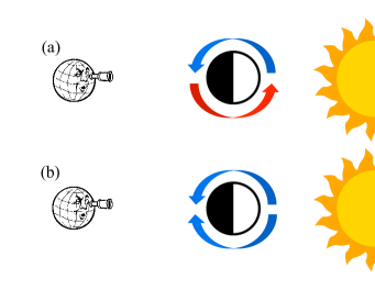
Figure 1.— Schematic implications of atmospheric circulation for Doppler measurements of a hot Jupiter observed in transit. Planet’s host star is depicted at right, planet (viewed looking down over north pole) is at the center, and Earth is at the left. (a): In the presence of zonal jets, air flows along latitude circles (colored arrows), leading to airflow toward Earth along one terminator (blue arrow) and away from Earth along the other (red arrow). A Doppler signature that is broadened, or in extreme cases may be bimodally split into blue- and redshifted components, results. (b): When zonal jets are damped, air flows primarily from day to night at low pressure, leading to airflow toward Earth along both terminators (blue arrows). A primarily blueshifted Doppler signature results.

2.1. Jet-dominated regime

On rotating planets, the interaction of atmospheric turbulence with the anisotropy introduced by the meridional gradient of the Coriolis parameter (known as the $\beta$ effect) leads to the emergence of zonal jets, which often dominate the circulation (e.g., Rhines (1975, 1994), Williams (1978, 1979), Vallis & Maltrud (1993), Cho & Polvani (1996) Dritschel & McIntyre (2008); for recent reviews in the planetary context, see Vasavada & Showman (2005) and Showman et al. (2010)). When radiative forcing and friction are weak, the heating of air parcels as they cross the dayside or nightside will be too small to induce significant day-night temperature variations; the dominant driver of the flow will then be the meridional (latitudinal) gradient in the zonal-mean radiative heating. Such a flow will exhibit significant zonal symmetry in temperature and winds with the primary horizontal temperature variations occurring between the equator and the poles. For this regime to occur, the radiative timescale must be significantly longer than the timescale for air parcels to cross a hemisphere; the rotation rate must also be sufficiently fast, and the friction sufficiently weak. The speed and number of the zonal jets will depend on a zonal momentum balance between Coriolis accelerations acting on the mean-meridional circulation and eddy accelerations resulting from baroclinic and/or barotropic instabilities, if any.

When the radiative forcing is sufficiently strong, as expected for typical hot Jupiters, large day-night heating contrasts will occur. As shown by Showman & Polvani (2011), such heating contrasts induce standing, planetary-scale Rossby and Kelvin waves. For typical hot Jupiter parameters, these waves cause an equatorward flux of eddy angular momentum that drives a superrotating (eastward) jet at the equator (Showman & Polvani, 2011). This provides a theoretical explanation for the near-ubiquitous emergence of eastward equatorial jets in atmospheric circulation models of hot Jupiters.

In these jet-dominated regimes (Fig. 1a), air along the terminator—as seen during transit—flows toward Earth in some regions and away from Earth in others. This leads to a Doppler signature where spectral lines are broadened, with minimal overall shift in the central wavelength. In extreme cases the Doppler signature may be split into distinct, superposed blue- and redshifted velocity peaks.

2.2. Suppression of jets by damping

The presence of sufficiently strong radiative or frictional damping can suppress the formation of zonal jets, leading to a circulation that at high altitudes is dominated by day-to-night flow rather than jets that are quasi-symmetric in longitude (Fig. 1b). Here, we demonstrate the conditions under which the mechanisms of Showman & Polvani (2011) are suppressed.

Showman & Polvani (2011) identified two specific mechanisms for the emergence of equatorial superrotation in models of synchronously rotating hot Jupiters. We consider each in turn.

2.2.1 Differential zonal wave propagation

As described above, the day-night thermal forcing on a highly irradiated, synchronously rotating planet generates standing, planetary-scale Rossby and Kelvin waves. The Kelvin waves straddle the equator while the Rossby waves exhibit pressure perturbations peaking in the midlatitudes for typical hot Jupiter parameters. The (group) propagation of Kelvin waves is to the east while that of long Rossby waves is to the west; this differential zonal propagation induces an eastward phase shift of the standing wave pattern near the equator and a westward phase shift at high latitudes. The result is a pattern of eddy velocities (northwest-southeast in the northern hemisphere and southwest-northeast in the southern hemisphere) that causes an equatorward flux of eddy angular momentum.

If the radiative or frictional timescales are significantly shorter than the time required for Kelvin and Rossby waves to propagate over a planetary radius, the waves are damped, inhibiting their zonal propagation and preventing the latitude-dependent phase shift necessary for the meridional angular momentum fluxes. Therefore, this mechanism for generating zonal jets is suppressed when radiative or frictional damping timescales are sufficiently short. The Kelvin-wave dispersion relation in the primitive equations

$$\omega={Nk\over\left({m^{2}+{1\over 4H^{2}}}\right)^{1/2}}$$ (1)

where $\omega$ is wave frequency, $k>0$ and $m$ are zonal and vertical wavenumbers, respectively, $N$ is the Brunt-Vaisala frequency, and $H$ is the scale height. The fastest propagation speeds occur in the limit of long vertical wavelength ($m\to 0$), which yields $\omega=2NHk$ and thus phase and group propagation velocities of $2NH$. The propagation time across a hemisphere is thus roughly $a/NH$, where $a$ is the planetary radius. We thus expect this jet-driving mechanism to be inhibited when

$$\tau_{\rm rad}\ll{a\over NH}\quad{\rm or}\quad\tau_{\rm drag}\ll{a\over NH}.$$ (2)

For typical hot-Jupiter parameters ($a=10^{8}\rm\,m$, $H\approx 400\rm\,km$, and $N\approx 3\times 10^{-3}\rm\,s^{-1}$ appropriate to a vertically isothermal temperature profile for a gravity of $10\rm\,m\,s^{-2}$ and specific heat at constant pressure of $1.3\times 10^{4}\rm\,J\,kg^{-1}\,K^{-1}$), we obtain $a/NH\sim 10^{5}\sec$. Thus, this mechanism should be inhibited when the radiative or drag time scales are much shorter than $\sim$$10^{5}\rm\,s$.

2.2.2 Multi-way force balance

Even when the radiative timescale is extremely short and zonal propagation of Rossby and Kelvin waves is inhibited, an eddy-velocity pattern that promotes equatorial superrotation can occur under some conditions. As pointed out by Showman & Polvani (2011) in the context of linear solutions, a three-way horizontal force balance between pressure-gradient, Coriolis, and frictional drag forces can lead to eddy velocities tilted northwest-southeast in the northern hemisphere and southwest-northeast in the southern hemisphere if the drag and Coriolis forces are comparable. This occurs because drag generally points opposite to the wind direction, whereas the Coriolis force points to the right (left) of the wind in the northern (southern) hemisphere. When these two forces are comparable, balancing them with the pressure-gradient force requires that the horizontal wind rotates clockwise of the day-night pressure-gradient force in the northern hemisphere and counterclockwise of it in the southern hemisphere (Figure 2). In the limit of short $\tau_{\rm rad}$ when the horizontal pressure-gradient force points from day to night, these arguments imply that, at low latitudes, the eddy velocities tilt northwest-southeast in the northern hemisphere and southwest-northeast in the southern hemisphere (Figure 2; see Showman & Polvani, 2011, Appendix D, for an analytic demonstration).

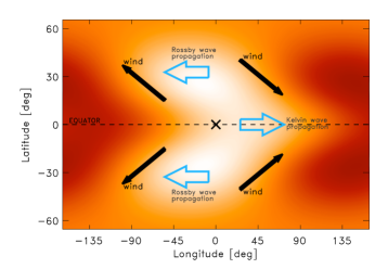
Figure 2.— Schematic illustrating two mechanisms for driving equatorial superrotation on a hot Jupiter from Showman & Polvani (2011). (a) The day-night thermal forcing generates standing, planetary-scale Kelvin and Rossby waves. Differential zonal (east-west) propagation of these waves—Kelvin wave to the east and Rossby waves to the west—leads to an eastward displacement of the thermal structure at the equator and a westward displacement at midlatitudes and, in turn, eddy velocities that tilt northwest-southeast in the northern hemisphere and southwest-northeast in the southern hemisphere. This pattern leads to an equatorward flux of eddy momentum and the emergence of equatorial superrotation. (b). Even when radiative forcing is sufficiently strong to suppress the differential zonal thermal offsets just mentioned, a three-way force balance between pressure-gradient, Coriolis, and drag forces can lead to equatorward-eastward and poleward-westward velocity tilts, thereby driving equatorial superrotation. Light regions indicate the dayside (with the substellar point marked by an $\times$), and darker regions indicate the nightside. When the radiative time constant is short over a broad range of pressures, the pressure-gradient force points from day to night (long gray open arrows). In the linear limit, the pressure-gradient force is balanced by the sum of drag (short gray open arrows) and Coriolis forces (short white open arrows). The fact that the Coriolis force points to the right (left) of the wind vector in the northern (southern) hemisphere, and that drag typically points in the opposite direction of the wind itself, implies that drag and Coriolis forces will exhibit orientations qualitatively similar to those drawn in the figure when their amplitudes are comparable. This three-way force balance therefore implies that the wind vectors themselves exhibit an orientation which is rotated clockwise relative to $-\nabla p$ in the northern hemisphere and counterclockwise relative to $-\nabla p$ in the southern hemisphere. The figure makes clear that, at low latitudes, these eddy wind-vector orientations correspond to northwest-southeast tilts in the northern hemisphere and southwest-northeast tilts in the southern hemisphere. The result would be the equatorward transport of eddy angular momentum and the development of equatorial superrotation.

Even when frictional drag is too weak to play an important role in the force balance, a similar three-way balance between pressure-gradient, Coriolis, and advection forces can under appropriate conditions lead to velocity tilts that promote equatorial superrotation. As air flows from day to night, the Coriolis force will deflect the trajectory of the airflow to the right of the pressure-gradient force in the northern hemisphere and to the left of it in the southern hemisphere. When the pressure-gradient force per mass, Coriolis force per mass, and advective acceleration are all comparable, as expected under the Rossby number $Ro\sim 1$ conditions typical of hot Jupiters, then the deflection will be substantial. In the limit of short $\tau_{\rm rad}$ when the horizontal pressure-gradient force points from day to night, these arguments again imply that the eddy velocities tilt northwest-southeast in the northern hemisphere and southwest-northeast in the southern hemisphere.

Now consider the effect of damping on this mechanism. To the degree that the radiative timescale is short enough for temperatures to be close to radiative equilibrium, radiative damping will not inhibit this mechanism; however, strong frictional damping can prevent it from occurring. When the frictional force is much stronger than the Coriolis and advective forces, the horizontal force balance is no longer a multi-way force balance but rather becomes essentially a two-way balance between the pressure-gradient force and drag. In this case, winds simply flow down the pressure gradient from day to night. There is thus no overall tendency for prograde eddy-velocity tilts to develop, so the jet-pumping Reynolds stress, and the jets themselves, are weak.

To quantify the amplitude of drag needed for this transition to occur, consider a drag force per mass parameterized by $-{\bf v}/\tau_{\rm drag}$, where ${\bf v}$ is horizontal velocity and $\tau_{\rm drag}$ is the drag time constant. The drag force dominates over the Coriolis force when $\tau_{\rm drag}\ll f^{-1}$, where $f=2\Omega\sin\phi$ is the Coriolis parameter, $\Omega$ is the planetary rotation rate ($2\pi$ over the rotation period), and $\phi$ is latitude. Models of hot Jupiters predict flows whose dominant length scales are global, in which case the advective acceleration should scale as $U^{2}/a$, where $U$ is the characteristic horizontal wind speed. Drag will then dominate over the advection force when $\tau_{\rm drag}\ll(a/|\nabla\Phi|)^{1/2}$, where $|\nabla\Phi|$ is the characteristic amplitude of the horizontal day-night pressure-gradient force on isobars, given to order of magnitude by $|\nabla\Phi|\sim R\Delta T_{\rm horiz}\Delta\ln p/a$, where $R$ is the specific gas constant, $\Delta T_{\rm horiz}$ is the characteristic day-night temperature difference, and $\Delta\ln p$ is the range of $\ln p$ over which this temperature difference extends. For typical hot Jupiter parameters, both conditions imply drag dominance for $\tau_{\rm drag}\ll 10^{5}\sec$. When this condition is satisfied, the horizontal force balance is between the pressure-gradient and drag forces. As mentioned above, the resulting circulation at low pressure involves day-to-night flow with minimal zonal-mean eddy-momentum flux convergences in the meridional direction and weak zonal jets.

2.2.3 Direct damping of jets by friction

Frictional drag can also directly damp the zonal jets. A robust understanding of how drag influences the equilibrated jet speed—and hence a rigorous theoretical prediction of the amplitudes of drag needed to damp the jet—requires a detailed theory for the full, three-dimensional interactions of the global-scale planetary waves with the background flow, which is currently lacking. It is therefore not possible at present to provide a robust theoretical estimate of the amplitude of drag necessary to damp the zonal jets. Still, because the jets are fundamentally driven by global-scale waves that result from the day-night heating gradients (Showman & Polvani, 2011), and because the radiative time constant increases rapidly with depth, we expect that the magnitude of zonal-mean acceleration of the zonal-mean zonal wind varies strongly with depth. These arguments heuristically suggest that the necessary frictional damping times are less than a value ranging from $10^{4}\sec$ at low pressures of say $\lesssim$0.1 bar to $10^{6}\sec$ or more at pressures of several bars, below the infrared photosphere.

2.2.4 Recap

When the jets and the waves that generate them are suppressed, the planet will tend to exhibit a large day-night temperature difference at low pressure, resulting in a large horizontal pressure gradient force between day to night that will drive a day-night flow (modified by the Coriolis effect) at low pressure. In this regime, air flows toward Earth along most of the terminator, leading to a predominantly blueshifted Doppler signature during transit. Mass continuity requires the existence of a return flow from night to day in the deep atmosphere (below the regions sensed by Doppler transit measurements). Because the density at depth is much larger than that aloft, the velocities of this return flow can be small.

3. Test of the two regimes with an idealized model

We now demonstrate this transition from jet- to eddy-dominated circulation regimes in an idealized dynamical model. As in Showman & Polvani (2011), we consider a two-layer model, with constant densities in each layer; the upper layer represents the stratified, meteorologically active atmosphere and the lower layer represents the denser, quiescent deep interior. When the lower layer is taken to be infinitely deep and the lower-layer winds and pressure field are steady in time, the governing equations are the shallow-water equations for the flow in the upper layer:

$${d{\bf v}\over dt}+g\nabla h+f{\bf k}\times{\bf v}={\bf R}-{{\bf v}\over{\tau_{\rm drag}}}$$ (4)

$${\partial h\over\partial t}+\nabla\cdot({\bf v}h)={h_{\rm eq}(\lambda,\phi)-h\over\tau_{\rm rad}}\equiv Q$$ (5)

where ${\bf v}(\lambda,\phi,t)$ is horizontal velocity, $h(\lambda,\phi,t)$ is the upper layer thickness, $\lambda$ is longitude, $t$ time, $g$ is the (reduced) gravity, and $d/dt\equiv{\partial/\partial t}+{\bf v}\cdot\nabla$ is the material (total) derivative. The term ${\bf R}$ in Eq. (4) represents momentum advection between the layers; it is $-{\bf v}Q/h$ in regions of heating ($Q>0$) and zero in regions of cooling ($Q<0$). See Showman & Polvani (2011) for further discussion and interpretation of the equations.

In the context of a three-dimensional (3D) atmosphere, the boundary between the layers represents an atmospheric isentrope, and radiative heating/cooling, which transports mass between layers, is therefore represented as a mass source/sink, $Q$, in the upper-layer equations. We parameterize this as a Newtonian cooling that relaxes the thickness toward a radiative-equilibrium thickness, $h_{\rm eq}(\lambda,\phi)$, over a prescribed radiative time constant $\tau_{\rm rad}$. Here, we set

$$h_{\rm eq}(\lambda,\phi)=\begin{cases}H&{\rm on\;the\;nightside;}\\ H+\Delta h_{\rm eq}\cos\lambda\cos\phi&{\rm on\;the\;dayside}\end{cases}$$ (6)

where the substellar point is at $(\lambda,\phi)=(0^{\circ},0^{\circ})$. This expression incorporates the fact that, on the nightside, the radiative equilibrium temperature profile of a synchronously rotating hot Jupiter is constant (e.g., Showman et al., 2008), whereas on the dayside the radiative-equilibrium temperature increases from the terminator to the substellar point. An important property of Eq. (6) is that the zonal-mean radiative-equilibrium thickness, $\overline{h_{\rm eq}}$, is greater at the equator than the poles, reflecting the fact that a planet with zero obliquity (whether tidally locked or not) absorbs more sunlight at low latitudes than high latitudes. Note that Eq. (6) differs from the formulation of $h_{\rm eq}$ adopted by Showman & Polvani (2011), where $h_{\rm eq}$ was set to $H+\Delta h_{\rm eq}\cos\lambda\cos\phi$ across the entire planet (dayside and nightside).

In addition to radiation, we include frictional drag parameterized with Rayleigh friction, $-{\bf v}/\tau_{\rm drag}$, where $\tau_{\rm drag}$ is a specified drag timescale. The drag could result from vertical turbulent mixing (Li & Goodman, 2010), Lorentz-force braking (Perna et al., 2010), or other processes.

Our model formulation is identical to that described in Showman & Polvani (2011, Section 3.2) in all ways except for the prescription of $h_{\rm eq}(\lambda,\phi)$.

Parameters are chosen to be appropriate for hot Jupiters. We take $gH=4\times 10^{6}\rm\,m^{2}\sec^{-2}$ and set $\Delta h_{\rm eq}/H=1$, implying that the radiative-equilibrium temperatures vary by order-unity from nightside to dayside. We also take $\Omega=3.2\times 10^{-5}\sec^{-1}$ and $a=8.2\times 10^{7}\rm\,m$, implying a rotation period of 2.2 Earth days and radius of 1.15 Jupiter radii, similar to the values for HD 189733b. The radiative and frictional timescales are varied over a wide range to characterize the dynamical regime.

We solved Equations (4)–(5) in full spherical geometry using the Spectral Transform Shallow Water Model (STSWM) of Hack & Jakob (1992). The equations are integrated using a spectral truncation of T170, corresponding to a resolution of $0.7^{\circ}$ in longitude and latitude (i.e., a global grid of $512\times 256$ in longitude and latitude). All models were integrated until a steady state is reached.

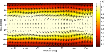
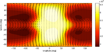
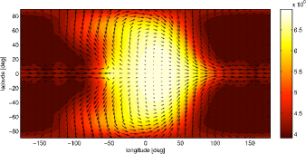
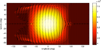
Figure 3.— Geopotential $gh$ (orange scale, units $\rm m^{2}\,s^{-2}$) and winds (arrows) for the equilibrated (steady-state) solutions to the shallow-water equations (Equations 4–5) in full spherical geometry assuming no upper-level drag ($\tau_{\rm drag}\to\infty$) and $\tau_{\rm rad}$=10, 1, 0.1, and 0.01 Earth days from top to bottom, respectively. Note the transition from a circulation dominated by zonally symmetric jets at long $\tau_{\rm rad}$ to one dominated by day-to-night flow at short $\tau_{\rm rad}$.

The solutions confirm our theoretical predictions of a regime transition. Figure 3 illustrates the equilibrated solutions for radiative time constants, $\tau_{\rm rad}$, of 10, 1, 0.1, and 0.01 days for the case where drag is turned off (i.e., $\tau_{\rm drag}\to\infty$). As expected, when the radiative time constant is long (10 days, panel (a)), jets dominate the circulation, with relatively weak eddies in comparison to the zonal-mean zonal winds. At intermediate values of the radiative time constant (1 and 0.1 days, panels (b) and (c)), the flow consists of strong jets and superposed eddies. At short values of the radiative time constant (0.01 days, panel (d)), the jets are relatively weak—though not absent—and day-to-night eddy flow dominates the circulation.

The dynamical behavior of this sequence can be understood as follows. When the radiative time constant is long (Figure 3(a)), the day-night thermal forcing is weak—air parcels experience only weak heating/cooling as they circulate from day to night—and the circulation is instead dominated by the equator-to-pole variation in the zonal-mean $h_{\rm eq}$ (i.e., by the zonal-mean radiative heating at low latitudes and cooling at high latitudes). At intermediate values of the radiative time constant (panels (b) and (c)), the day-night thermal forcing becomes sufficiently strong to generate a significant planetary wave response, and the eddy-momentum convergence induced by these waves generates equatorial superrotation via the mechanisms identified by Showman & Polvani (2011), particularly the differential zonal propagation of the standing Kelvin and Rossby waves. At short radiative time constant (panel (d)), such zonal propagation is inhibited but, as predicted by the theory in Section 2, the three-way force balance between pressure-gradient, Coriolis, and advection forces still generates prograde phase tilts in the velocities. Although, visually, the flow appears dominated primarily by day-to-night flow (Figure 3(d)), these phase tilts still drive superrotation near the equator, and even at higher latitudes the zonal-mean zonal wind remains a significant fraction of the eddy wind amplitude.

The transition from a regime dominated by jets to a regime dominated by day-to-night flow is even more striking when drag is included. Figure 4 shows a sequence of models with radiative time constants, $\tau_{\rm rad}$, of 10, 1, 0.1, and 0.01 days (as in Figure 3) but with $\tau_{\rm drag}=10\tau_{\rm rad}$ in all cases. Overall, the trend resembles that in Figure 3: at long radiative time constants (panel (a)), the flow is dominated by high-latitude, highly zonal jets; at intermediate radiative time constants (panel (b) and (c)), the flow is transitional, exhibiting strong eddies associated with the standing planetary-scale wave response to the day-night thermal forcing, and zonal jets driven by those eddies (cf Showman & Polvani, 2011); and at short radiative time constants (panel (d)), the Kelvin and Rossby waves are damped and the circulation consists almost entirely of day-to-night flow. As predicted by the theory in Section 2, drag in this case is strong enough to overwhelm the advection and Coriolis forces, leading to a two-way horizontal force balance between the pressure-gradient force and drag. As a result, there is no overall prograde phase tilt of the velocity pattern. The eddy forcing of the zonal-mean flow, and the jets themselves, are therefore weak.

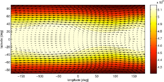
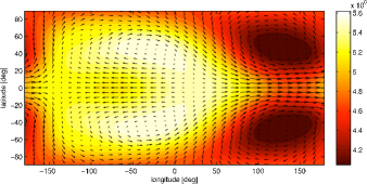
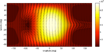
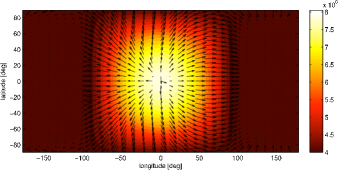
Figure 4.— Geopotential $gh$ (orange scale, units $\rm m^{2}\,s^{-2}$) and winds (arrows) for the equilibrated (steady-state) solutions to the shallow-water equations (Equations 4–5) in full spherical geometry assuming $\tau_{\rm drag}=10\tau_{\rm rad}$ and $\tau_{\rm rad}$=10, 1, 0.1, and 0.01 days from top to bottom, respectively. Note the transition from a circulation dominated by zonally symmetric jets at long $\tau_{\rm rad}$ to one dominated by day-to-night flow at short $\tau_{\rm rad}$.

To better characterize the dominance of jets versus day-night flow, we performed integrations over a complete grid including all possible combinations of 0.01, 0.1, 1, 10, and 100 days in $\tau_{\rm rad}$ and 0.1, 1, 10, 100, and $\infty$ days in $\tau_{\rm drag}$. The typical amplitude of the jets can be characterized by the root-mean-square of the zonal-mean zonal wind variation in latitude:

$$\overline{u}_{\rm rms}=\left[{1\over\pi}\int_{-\pi/2}^{\pi/2}\overline{u}(\phi)^{2}\,d\phi\right]^{1/2}$$ (7)

where the overbar denotes a zonal average. To characterize the amplitude of the eddies, we adopt a metric representing the variation of the zonal wind in longitude:

$$u_{\rm eddy}(\phi)=\left[{1\over 2\pi}\int_{-\pi}^{\pi}(u-\overline{u})^{2}\,d\lambda\right]^{1/2}$$ (8)

and then determine the root-mean-square variations of this quantity in latitude:

$$u_{\rm eddy,rms}=\left[{1\over\pi}\int_{-\pi/2}^{\pi/2}u_{\rm eddy}(\phi)^{2}\,d\phi\right]^{1/2}.$$ (9)

The ratio of $\overline{u}_{\rm rms}$ to $u_{\rm eddy,rms}$ then provies a measure of the relative dominance of jets versus day-night flow.

These calculations demonstrate that jets dominate when both the radiative and drag time constant are long, and that day-to-night eddy flow dominates when either time constant is very short. This is shown in Figure 5, which presents the ratio $\overline{u}_{\rm rms}/u_{\rm eddy,rms}$ versus $\tau_{\rm rad}$ and $\tau_{\rm drag}$. The dashed curve in panel (b), corresponding to $\overline{u}_{\rm rms}/u_{\rm eddy,rms}=1$, demarcates the approximate transition between regimes (jets dominate above and to the right of the curve, while day-night flow dominates below and to the left of the curve). Although extremely short values of either $\tau_{\rm rad}$ or $\tau_{\rm drag}$ are sufficient to ensure eddy-dominated flow, the trend of the transition differs for the two time constants. When drag is weak or absent, $\tau_{\rm rad}$ must be extremely short—less than 0.1 day—to ensure eddy- rather than jet-dominated flow (Figure 5). On the other hand, over a wide range of $\tau_{\rm rad}$ values, $\tau_{\rm drag}$ need only be less than $\sim$3 days to ensure eddy-dominated flow. The transition between jet and eddy-dominated regimes as a function of drag occurs more sharply when $\tau_{\rm rad}$ is large than when it is small.

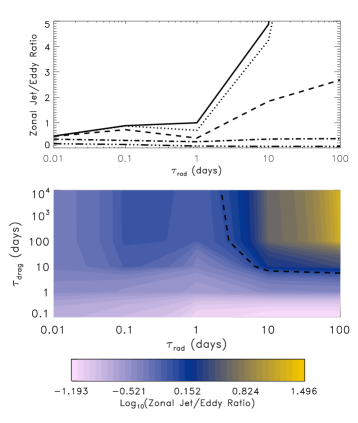
Figure 5.— Ratio $\overline{u}_{\rm rms}/u_{\rm eddy,rms}$, characterizing the ratio of jets to eddies, versus $\tau_{\rm rad}$ and $\tau_{\rm drag}$. Top: triple-dashed-dotted, dashed-dotted, dashed, dotted, and solid curves depict results from models with $\tau_{\rm drag}$ values of 0.1, 1, 10, 100 days, and infinite (i.e., no drag in the upper layer), respectively. Bottom: Two-dimensional representation of the same data. Colorscale depicts $\log_{\rm 10}(\overline{u}_{\rm rms}/u_{\rm eddy,rms})$ with even log-spacing of the contour intervals. Values of $\overline{u}_{\rm rms}/u_{\rm eddy,rms}$ range from 0.06 (i.e., $10^{-1.193}$) to 31 (i.e., $10^{1.496}$). The dashed black contour denotes $\overline{u}_{\rm rms}/u_{\rm eddy,rms}=1$ (i.e., $\log_{\rm 10}(\overline{u}_{\rm rms}/u_{\rm eddy,rms})=0$), giving an approximate demarcation between the jet- and eddy-dominated regimes. Jets dominate when both $\tau_{\rm rad}$ and $\tau_{\rm drag}$ are long, and eddies (essentially day-night flow) dominate when either time constant becomes very short.

4. Three-dimensional models

We now demonstrate this regime shift in three-dimensional atmospheric circulation models including realistic radiative transfer. GJ 436b, HD 189733b, and HD 209458b are selected as examples that bracket a large range in stellar irradiation and yet are relatively easily observable, hence representing good targets for Doppler characterization.

4.1. Model setup

We solve the radiation hydrodynamics equations using the Substellar and Planetary Atmospheric Circulation and Radiation (SPARC) model of Showman et al. (2009). This model couples the dynamical core of the MITgcm (Adcroft et al., 2004), which solves the primitive equations of meteorology in global, spherical geometry, using pressure as a vertical coordinate, to the state-of-the-art, nongray radiative transfer scheme of Marley & McKay (1999), which solves the multi-stream radiative transfer equations using the correlated-$k$ method to treat the wavelength dependence of the opacities. Here, we use a two-stream implementation of this model. To date, this is the only circulation model of hot Jupiters to include a realistic radiative transfer solver, which is necessary for accurate determination of heating rates, temperatures, and flowfield. The composition and therefore opacities in hot-Jupiter atmospheres are uncertain. Here, gaseous opacities are calculated assuming local chemical equilibrium for a specified atmospheric metallicity, allowing for rainout of any condensates. We neglect any opacity due to clouds or hazes.

Model parameters are summarized in Table 1. Although the atmosphere of GJ 436b is likely enriched in heavy elements (Spiegel et al., 2010; Lewis et al., 2010; Madhusudhan & Seager, 2011), solar metallicity represents a reasonable baseline for HD 189733b and HD 209458b, and to establish the effect of differing stellar flux at constant metallicity we therefore adopt solar metallicity for the gas opacities in our nominal models of all three planets. To bracket the range of plausible metallicities, we also explore a model of GJ 436b with 50 times solar metallicity. For HD 189733b and GJ 436b, we neglect opacity due to strong visible-wavelength absorbers such as TiO and VO, as TiO and VO are not expected for these cooler planets. For HD 209458b, secondary-eclipse measurements suggest the presence of a stratosphere (Knutson et al., 2008), and we therefore include TiO and VO opacity for this planet, which allows a thermal inversion due to the large visible-wavelength opacity of these species (Hubeny et al., 2003; Fortney et al., 2008; Showman et al., 2009). While debate exists about the ability of TiO to remain in the atmosphere (Showman et al., 2009; Spiegel et al., 2009), our present purpose is simply to use TiO as a proxy for any chemical species that strongly absorbs in the visible wavelengths and hence allows a stratosphere to exist; other strong visible-wavelength absorbers would exert qualitatively similar effects. Synchronous rotation is assumed for HD 189733b and HD 209458b (with a substellar longitude perpetually at $0^{\circ}$); the rotation of GJ 436b, however, is assumed to be pseudosychronized with its slightly eccentric orbit (Lewis et al., 2010). The obliquity of all models is zero so that the substellar point lies along the equator.

Table 1Model Parameters

	GJ 436b	HD 189733b	HD 209458b
radius (m)	$2.69\times 10^{7}$	$8.2396\times 10^{7}$	$9.437\times 10^{7}$
rotation period (days)	2.3285	2.2	3.5
gravity ($\rm m\,s^{-2}$)	12.79	21.4	9.36
$p_{\rm base}(\rm bars)$	200	200	200
$p_{\rm top}(\rm bars)$	$2\times 10^{-5}$	$2\times 10^{-6}$	$2\times 10^{-6}$
$N_{r}$	47	53	53
metallicity (solar)	1 and 50	1	1

Our nominal models do not include explicit frictional drag in the upper levels. However, several frictional processes may be important for hot Jupiters, including vertical turbulent mixing (Li & Goodman, 2010), breaking small-scale gravity waves (Watkins & Cho, 2010), and magnetohydrodynamic drag (Perna et al., 2010). The latter may be particularly important for hot planets such as HD 209458b. Accordingly, we additionally present a sequence of HD 209458b integrations that include frictional drag, which we crudely parameterize as a linear relaxation of the zonal and meridional velocities toward zero over a prescribed drag time constant, $\tau_{\rm drag}$. Within any given model, we treat $\tau_{\rm drag}$ as a constant everywhere within the domain. This is not a rigorous representation of drag (for example, Lorentz forces will vary greatly from dayside to nightside and may act anisotropically on the zonal and meridional winds); still, the approach allows a straightforward evaluation of how drag of a given strength alters the circulation.

For all three planets, we solve the equations on the cubed-sphere grid using a horizontal resolution of C32, corresponding to an approximate global resolution of $128\times 64$ in longitude and latitude. The lowermost $N_{r}-1$ vertical levels are evenly spaced in log-pressure from an average basal pressure $p_{\rm base}$ of 200 bars to a top pressure, $p_{\rm top}$, of $20\,\mu$bars for GJ 436b and $2\,\mu$bars for HD 189733b and HD 209458b. The uppermost model level extends from a pressure of $p_{\rm top}$ to zero. Our models of GJ 436b and HD 189733b were originally presented in Lewis et al. (2010) and Fortney et al. (2010), respectively, while for HD 204958b we present new models here. These new integrations adopt 11 opacity bins in our correlated-$k$ scheme; detailed tests show that this 11-bin scheme produces net radiative fluxes, heating rates, and atmospheric circulations very similar to those of the 30-bin models (see Kataria et al., 2012). We integrate these models until they reach an essentially steady flow configuration at pressures $<1\,$bar, corresponding to integration times typically ranging from one to four thousand Earth days, depending on the model.

4.2. Results: nominal models

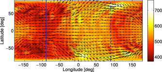
Figure 6.— Global temperature (orange scale) and winds (arrows) for a sequence of 3D SPARC/MITgcm models at a pressure of 0.1 mbar, where Doppler measurements are likely to sense. Panels (a), (b), (c), and (d) show solar-metallicity GJ 436b, $50\times$ solar GJ 436b, solar-metallicity HD 189733b, and solar-metallicity HD 209458b models, respectively. The vertical blue solid and dashed lines show the location of the terminators $90^{\circ}$ west and east of the substellar longitude, respectively. The substellar point is at longitude $0^{\circ}$ in all panels. The models show a gradual transition from a circulation dominated by zonal jets (top) to one dominated by day-night flow at low pressure (bottom).

Our nominal, three-dimensional models exhibit a fundamental transition in the upper-atmospheric behavior—at pressures where Doppler measurements are likely to sense—as stellar insolation increases from modest (for GJ 436b) to intermediate (for HD 189733b) to large (for HD 209458b). This is illustrated in Figures 6 and 7. Figure 6 shows temperature and winds over the globe for models of GJ 436b, HD 189733b, and HD 209458b. Figure 7 presents histograms of the fraction of terminator arc length versus terminator zonal-wind speed for these same models, which gives an approximate sense of how a discrete spectral line would be split, shifted, or smeared in frequency due to the Doppler shift of zonal winds along the terminator. To isolate the effect of dynamics, the contribution of planetary rotation to the velocity is not included in Figure 7, although we will return to its effects subsequently.

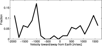
Figure 7.— Histograms showing the fraction of the full, $360^{\circ}$ terminator, at a pressure of 0.1 mbar, flowing at various wind speeds toward or away from Earth for the four models presented in Figure 6. (To isolate the dynamical contribution, this does not include the contribution of planetary rotation to the inertial-frame velocity.) Negatives values are toward Earth and positive values are away from Earth. Panels (a), (b), (c), and (d) show solar-metallicity GJ 436b, $50\times$ solar GJ 436b, solar-metallicity HD 189733b, and solar-metallicity HD 209458b models, respectively. This gives a crude sense of the dynamical contribution to the Doppler splitting of a discrete spectral line. The models exhibit a transition from flows that exhibit both blue- and red-shifted components (top) to a flow whose Doppler signature would be predominantly blueshifted (bottom).

In the case of solar-metallicity GJ 436b (Figure 6a), the predominant dynamical feature is a broad superrotating (eastward) jet that extends over all longitudes and in latitude almost from pole to pole. The jet exhibits significant wave activity, manifesting as small-scale fluctuations in temperature and zonal wind, particularly at the high latitudes of both hemispheres where the zonal-mean zonal winds peak. Nevertheless, the model exhibits little tendency toward a zonal-wavenumber-one pattern that would be associated with a predominant day-to-night flow. Save for small regions near the poles, the zonal winds at low pressure are everywhere eastward, implying that, during transit, the zonal winds flow away from Earth along the leading limb and toward Earth along the trailing limb. This would lead to almost equal blueshifted and redshifted Doppler components, with a relative minimum near zero Doppler shift (Figure 7a).

Next consider HD 189733b (Figure 6c). The model again exhibits a superrotating equatorial jet, which is fast across most of the nightside—achieving eastward speeds of $4\rm\,km\,s^{-1}$—but slows down considerably over the dayside, reaching zero speed near the substellar point. Despite this variation, the zonal winds within the jet (latitudes equatorward of $60^{\circ}$) are eastward along both terminators. In contrast, the high-latitude zonal wind (poleward of $60^{\circ}$ latitude) is westward along the western terminator and eastward along the eastern terminator, as expected for day-to-night flow. As seen during transit, along the trailing limb, the zonal winds flow toward Earth. Along the leading limb, they flow toward Earth poleward of $60^{\circ}$ latitude and away from Earth equatorward of $60^{\circ}$ latitude. Spectral lines would thus exhibit a broadened or bimodal character, with the blueshifted component considerably stronger than the redshifted component (Figure 7c). HD 189733b is thus a transitional case between the two regimes discussed in Section 2.

In the case of HD 209458b (Figure 6d), the strong superrotating jet continues to exist, but at and west of the western terminator it is confined substantially closer to the equator than in our GJ 436b or HD 189733b models. Poleward of $\sim$$30^{\circ}$ latitude on the western terminator, and everywhere along the eastern terminator, the airflow direction is from day to night. This implies that, as seen during transit, the trailing limb exhibits zonal winds toward Earth. The leading limb exhibits zonal winds that are toward Earth poleward of $\sim$$30^{\circ}$ latitude and away from Earth equatorward of $\sim$$30^{\circ}$ latitude. This would lead to Doppler shifts that are almost entirely blueshifted (Figure 7d).

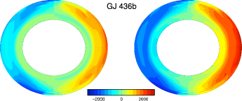
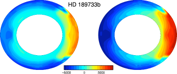
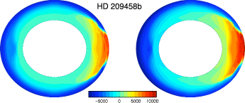
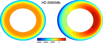
Figure 8.— Winds toward or away from Earth (colorscale, $\rm m\,s^{-1}$) along the full, $360^{\circ}$ terminator in a sequence of models as viewed during the center of transit. Colorscale is such that red (positive) represents redshifted velocities while blue (negative) represents blueshifted velocities. The radial coordinate represents log pressure, and the plotted range is from 200 bars at the inside to $2\,\mu$bar at the outside. The first, second, and third rows show our solar-metallicity nominal models of GJ 436b, HD 189733b, and HD 209458b, respectively. The fourth row shows our model of HD 209458b where frictional drag is imposed with a drag time constant of $10^{4}\rm\,s$. For each model, the left panel shows the winds alone, and the right panel shows the sum of the winds and the planet’s rotation. From top to bottom, the transition from high-altitude velocities that have both blue and redshifted components to velocities that are entirely blueshifted is clearly evident.

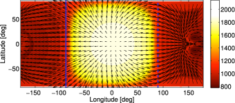
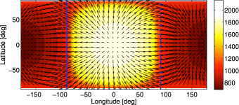
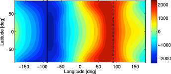
Figure 9.— Temperature and winds at 0.1 mbar pressure in models of HD 209458b with frictional drag. Left: a model with a drag time constant of $3\times 10^{4}\,$s. Right: a model with a drag time constant of $10^{4}\,$s. Top panels show temperature in K (orange scale) and winds (arrows). Bottom panels show zonal wind in $\rm m\,s^{-1}$. In the case with weaker drag, an equatorial jet extends partway across the nightside, but the jet is damped out in the case with stronger drag. Vertical solid and dashed lines show the terminators.

To summarize, these models exhibit a transition from a circulation dominated by zonal jets at modest insolation (GJ 436b) to one dominated by day-night flow at high insolation (HD 209458b). Qualitatively, this transition matches well the predictions from our theory in Section 2—as the stellar insolation increases, the effective radiative timescale decreases, and this damps the standing planetary-scale Rossby and Kelvin waves, limiting their ability to drive a dominant zonal flow and leading to a circulation comprised primarily of day-to-night flow at low pressure. We emphasize that the models in Figures 6–7 do not contain frictional drag at the low pressures sensed by remote measurements, and so the only source of damping is the radiation (as well as the Shapiro filter, which exerts minimal effect at large scales). The models show that the regime transition occurs very gradually as stellar insolation is varied (Figures 6a–d). This is also consistent with theoretical expectations; as shown in Figure 5, when large-scale drag is absent, the radiative time constant must be decreased by over a factor of $\sim$30 (from $\sim$3 days to less than 0.1 day) to force the flow from the jet-dominated to eddy-dominated regime. Moreover, as discussed in Section 2, damping through radiation alone can inhibit differential zonal propagation of the planetary-scale waves, but the multi-way horizontal force balance between pressure-gradient, Coriolis, and advective forces can still produce prograde phase tilts near the equator. Thus, we still expect a narrow equatorial jet over at least some longitudes. This can be seen in the nonlinear shallow-water solutions (see Figure 3(d)) and also explains the continuing existence of a narrow equatorial jet even for extreme radiative forcing in the 3D models (Figure 6(d)).

This regime transition manifests clearly in plots of terminator winds. Figure 8 shows the wind component projected along the line of sight to Earth at the terminator for a sequence of models. Red represents velocities away from Earth (hence redshifted) while blue represents velocities toward Earth (hence blueshifted). The first, second, and third rows of Figure 8 show our nominal models of GJ 436b, HD 189733b, and HD 209458b, while the fourth row depicts our model of HD 209458b adopting frictional drag with $\tau_{\rm drag}=10^{4}\rm\,s$. For GJ 436b, the leading limb is redshifted while the trailing limb is blueshifted. For HD 189733b, the redshifted portion—corresponding to the equatorial jet—is confined to the low and midlatitudes on the leading limb. As a result, at high altitudes, only about one-quarter of the limb is redshifted, while about three-quarters is blueshifted. For our nominal HD 209458b model, the confinement of the equatorial jet to low latitudes on the leading limb is even stronger, such that only about $\sim$10% of the high-altitude limb is redshifted while $\sim$90% is blueshifted. In the HD 209458b model with frictional drag, the high-altitude winds are blueshifted over the entire terminator, completing the transition from a circulation dominated by jets to one dominated by high-altitude day-to-night flow.

The regime transition discussed here is affected not only by the stellar insolation but also the atmospheric metallicity. Larger metallicities imply larger gaseous opacities (due to the increased abundance of H₂O, CO, and CH₄), and this moves the photosphere to lower pressures (cf Spiegel et al., 2010; Lewis et al., 2010), implying that the bulk of the starlight is then absorbed in a region with very little atmospheric mass. As a result, increasing the atmospheric metallicity enhances the dayside heating and nightside cooling per mass at the photosphere even when the stellar insolation remains unchanged. The effects of this are illustrated in Figure 6b, which shows a GJ 436b model identical to that in Figure 6a except that the metallicity is 50 times solar (Lewis et al., 2010). Because of the greater absorption of stellar radiation at high levels, the atmosphere exhibits a large day-night temperature difference and significant zonal-wavenumber-one structure in the zonal wind, with strong longitudinal variations in the equatorial jet reminiscent of that in our HD 189733b model (compare Figures 6(b) and (c)). Although eastward flow still dominates along most of the terminator, as in the solar-metallicity GJ 436b model, the western terminator exhibits westward flow within $\sim$$30^{\circ}$ latitude of the pole. Spectral lines as seen during transit still exhibit bimodel blue and redshifts, but the blueshifts are now slightly more dominant (Figure 7b).

Although we have focused on the existence of a regime transition in models with differing stellar fluxes, it is worth emphasizing that the same transition often occurs within a given model from low pressure to high pressure. Generally speaking, the radiative time constants are short at low pressure and long at high pressure (Iro et al., 2005; Showman et al., 2008). The theory presented here therefore predicts that, as long as the incident stellar flux is sufficiently high and frictional drag is sufficiently weak, the air should transition from a day-to-night flow pattern at low pressure to a jet-dominated zonal flow at high pressures. Just such a pattern is seen in many published 3D hot Jupiter models (e.g., Cooper & Showman, 2005, 2006; Showman et al., 2008, 2009; Rauscher & Menou, 2010; Heng et al., 2011b). Note, however, that if the incident stellar flux is sufficiently low (and the drag is very weak), the atmosphere may be in a regime of jet-dominated flow throughout; on the other hand, if frictional drag is sufficiently strong, jets may be unable to form at all, and the atmosphere may be in a regime of day-night flow aloft with a very weak return flow at depth.

4.3. Results: influence of drag

We now consider the effect of frictional drag in 3D models. As discussed in Section 2, sufficiently strong frictional drag (i) damps the standing planetary-scale waves that are the natural response to the day-night heating gradient, and (ii) drives the horizontal force balance into a two-way balance between pressure-gradient and drag forces, both of which inhibit the development of prograde phase tilts in the eddy velocities and in turn the pumping of zonal jets, and, finally (iii) directly damps the zonal jets. Thus, we expect that an atmosphere with sufficiently strong frictional drag will lack zonal jets and that its circulation will instead consist primarily of day-to-night flow at high altitude, with return flows at depth. Figure 9 illustrates this for solar-metallicity models of HD 209458b where Rayleigh drag is implemented with time constants of $3\times 10^{4}\rm\,s$ (left column) and $10^{4}\rm\,s$ (right column). As predicted, the air at 0.1 mbar flows directly from dayside to nightside over both terminators. The model with $\tau_{\rm drag}=3\times 10^{4}\rm\,s$ exhibits a remnant equatorial jet on the nightside that extends from the eastern terminator to the antistellar point. Because the stronger frictional drag damps it out, the model with $\tau_{\rm drag}=10^{4}\rm\,s$ lacks such a jet, and the flow exhibits only modest asymmetry (due to the $\beta$ effect) between the western and eastern terminators. Doppler lines would be entirely blueshifted in both cases.

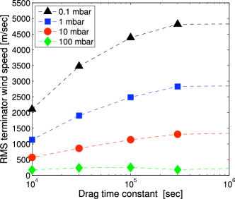
Figure 10.— Steady-state root-mean-square wind speeds at the terminator versus frictional drag time constant from a sequence of HD 209458b models including drag. For each 3D model, performed for a given drag time constant, the root-mean-square wind speeds—calculated along the terminator—are shown at pressures of 0.1, 1, 10, and 100 mbar. For these models the speeds generally represent day-night flow. The dashed lines to the right of the rightmost points are connecting to the model with no drag in the upper atmosphere ($\tau_{\rm drag}\to\infty$), where the rms terminator wind speed is 5200, 3800, 2600, and $1900\rm\,m\,s^{-1}$ at 0.1, 1, 10, and 100 mbar, respectively. The equilibrated speeds depend significantly on the drag time constant and, within a given model, on pressure.

Friction affects not only the qualitative circulation regime (e.g., existence or lack of zonal jets) but also the speed of the high-altitude flow between day and night. Figure 10 shows the root-mean-square zonal wind speeds at the terminator for a sequence of HD 209458b models with differing drag time constants. All of these runs are in the same regime as the model in Figure 9, where day-to-night flow dominates at low pressure. When $\tau_{\rm drag}$ is sufficiently long, the flow speeds are independent of the drag time constant, but they start to decrease when $\tau_{\rm drag}$ is sufficiently short. When drag is absent in the upper atmosphere, our HD 209458b model equilibrates to an rms terminator wind speed of $5.2\rm\,km\,s^{-1}$ at 0.1 mbar, decreasing with depth to $3.8$, $2.6$, and $1.9\rm\,km\,s^{-1}$ at 1, 10, and 100 mbar, respectively. As shown in Figure 10, the addition of weak drag ($\tau_{\rm drag}=3\times 10^{5}\rm\,s$) exerts only a modest effect on the day-night flow speeds at pressures $\lesssim 10\rm\,mbar$. Drag time constants $\tau_{\rm drag}\lesssim 10^{5}\rm\,s$ start to matter significantly in the upper atmosphere, however; for example, for $\tau_{\rm drag}=10^{4}\rm\,s$, the rms terminator speeds are $2.1$, $1.1$, $0.6$, and $0.2\rm\,km\,s^{-1}$ at 0.1, 1, 10, and 100 mbar—significantly less than the equilibrated speeds in the absence of upper-level drag.

The above results suggest that the amplitude of the observed Doppler shift can place constraints on the strength of frictional drag in the upper atmospheres of hot Jupiters. Snellen et al. (2010)’s inference of winds on HD 209458b is tentative but, at face value, suggests wind speeds toward Earth of $2\pm 1\rm\,km\,s^{-1}$. Snellen et al. (2010) suggest that their measurements are sensing pressure levels of 0.01–0.1 mbar. At these levels, the winds in our models equilibrate to $\sim$4–$6\rm\,km\,s^{-1}$ when drag is weak, and Figure 10 shows that reducing the wind speed to $2\rm\,km\,s^{-1}$ requires drag time constants potentially as short as $\sim$$10^{4}\rm\,s$. This hints that strong frictional drag processes may operate in the atmosphere of HD 209458b. But caution is warranted: Figure 10 also demonstrates that the rms terminator wind speeds also depend strongly on pressure within any given model; therefore, making robust inferences about drag amplitudes from observed Doppler shifts requires extremely careful and accurate estimates of the pressure levels being probed. This may be a challenge, at least until the composition and hence wavelength-dependent opacity of hot Jupiters are better understood. If the Snellen et al. (2010) measurements are actually sensing deeper pressures of $\sim$$10\rm\,mbar$, say, then explaining their 2-$\rm km\,s^{-1}$ signal would require little if any drag in the observable atmosphere.

In light of Figure 10, it is interesting to briefly comment on the pressures being probed in transmission spectra computed from our models. In Section 5, we will present transmission spectra for our 3D models computed self-consistently from high-spectral-resolution versions of the same opacities used to integrate the GCM. These calculations indicate that, in the $K$-band region considered by Snellen et al., our synthetic transmission spectra probe pressures ranging from $\sim$10 mbar in the continuum between spectral lines to less than $\sim$0.1 mbar at line cores. It is the Doppler shifts of the spectral lines that are observable—the Doppler shift of the continuum, if any, is almost undetectable since the absorption depends only weakly on wavelength there. As a result, the overall Doppler signal detected in a spectral cross-correlation is heavily weighted toward the Doppler shift of the spectral lines. We find that, when cross-correlating our synthetic transmission spectra with template spectra, our models of HD 209458b primarily probe the atmospheric winds at pressures of 0.1 to 1 mbar.

The qualitative dependence of terminator wind speed on the drag time constant—illustrated in Figure 10—can be understood analytically. To order of magnitude, the horizontal pressure gradient force in pressure coordinates between day and night can be written $R\Delta T_{\rm horiz}\Delta\ln p/a$. This is balanced by some combination of advection, of magnitude $U^{2}/a$, Coriolis force, of magnitude $fU$, and drag, of magnitude $U/\tau_{\rm drag}$. Drag will dominate when $\tau_{\rm drag}\lesssim f^{-1}$ and when $U/\tau_{\rm drag}\gtrsim U^{2}/a$, which requires $\tau_{\rm drag}\ll(a/|\nabla\Phi|)^{1/2}$, equivalent to the requirement that $\tau_{\rm drag}\ll a/(R\Delta T_{\rm horiz}\Delta\ln p)^{1/2}$. As long as these conditions are satisfied, we can balance drag against the pressure-gradient force. Solving for $\tau_{\rm drag}$ then implies that the amplitude of drag necessary to obtain a wind speed $U$ is

$$\tau_{\rm drag}\sim{Ua\over R\Delta T_{\rm horiz}\Delta\ln p}$$ (10)

Inserting parameters appropriate to the 0.1 mbar level on HD 209458b ($a\sim 10^{8}\rm\,m$, $R\sim 3700\rm\,J\,kg^{-1}\,K^{-1}$, $\Delta T_{\rm horiz}\sim 1000\rm\,K$, and $\Delta\ln p\sim 5$), and adopting $U\sim 2\rm\,km\,s^{-1}$ motivated by the Snellen et al. measurement of HD 209458b, we obtain $\tau_{\rm drag}\sim 10^{4}\rm\,s$. This value agrees well with the strength of drag needed in our 3D model intregrations to achieve a speed of $2\rm\,km\,s^{-1}$ at the 0.1 mbar level (leftmost black triangle in Figure 10).

5. Transmission Spectrum Calculations

To quantify the implications for observations, in this section we present theoretical transmission spectra from our 3D models demonstrating the influence of Doppler shifts due to atmospheric winds. These spectra illustrate how the dynamical regime shifts described in the preceding sections manifest in transit spectra.

5.1. Methods

We have previously developed a code to compute the transmission spectrum of transiting planet atmospheres, which we extend here to include Doppler shifts due to atmospheric winds. The first generation of the code, which used one-dimensional atmospheric pressure-temperature (p-T) profiles, is described in Hubbard et al. (2001) and Fortney et al. (2003). In Shabram et al. (2011) the one-dimensional (1D) version of the code was well-validated against the analytic transmission atmosphere model of Lecavelier Des Etangs et al. (2008). In Fortney et al. (2010) we implemented a method to calculate the transmission spectrum of fully 3D models.

The calculation of the absorption of light passing through the planet’s atmosphere is based on a simple physical picture. One can imagine a straight path through the planet’s atmosphere, parallel to the star-planet-observer axis, at an impact parameter $r$ from this axis. The gaseous optical depth $\tau_{\rm G}$, starting at the terminator and moving outward in one direction along this path, can be calculated via the equation:

$$\tau_{\rm G}=\int_{r}^{\infty}\frac{r^{\prime}\sigma(r^{\prime})n(r^{\prime})}{{(r^{\prime 2}-r^{2})}^{1/2}}\,dr^{\prime},$$ (11)

where $r^{\prime}$ is the distance between the local location in the atmosphere and the planetary center, $n$ is the local number density of molecules in the atmosphere, and $\sigma$ is the wavelength-dependent cross-section per molecule. Later we will discuss the role of winds leading to a Doppler shifted $\sigma$ away from rest wavelengths. We assume hydrostatic equilibrium with a gravitational acceleration that falls off with the inverse of the distance squared. The base radius is taken at a pressure of 10 bars, where the atmosphere is opaque, and this radius level is adjusted to yield the best fit to observations, where applicable. Here we define the wavelength-dependent transit radius as the radius where the total slant optical depth reaches 0.56, following Lecavelier Des Etangs et al. (2008). Additional detail and description can be found in Fortney et al. (2010), as the 3D setup here is the same as described in that paper.

For any particular column of atmosphere, hydrostatic equilibrium is assumed, and we use the given local p-T profile to interpolate in a pre-tabulated chemical equilibrium and opacity grid that extends out to 1 $\mu$bar. The equilibrium chemistry mixing ratios (Lodders, 1999; Lodders & Fegley, 2002, 2006) are paired with the opacity database (Freedman et al., 2008) to generate pressure - , temperature-, and wavelength-dependent absorption cross-sections that are used for that particular column. For a different column of atmosphere, with a different p-T profile, local pressures and temperatures will yield different mixing ratios and wavelength-dependent cross-sections.

We include the Doppler shifts due to the local atmospheric winds and planetary rotation when evaluating the opacity at any given region of the 3D grid. At high spectral resolution, rotation tends to cause a broadening of spectral lines (Spiegel et al., 2007), while the atmospheric wind speeds lead to absorption features that are Doppler shifted from their rest wavelengths (Snellen et al., 2010; Miller-Ricci Kempton & Rauscher, 2012). The cross section $\sigma$ is not evaluated at the rest wavelength, $\lambda_{0}$, but rather at the Doppler shifted value, $\lambda$, found via

$$\lambda=\lambda_{0}(1-\frac{v_{\rm los}}{c}),$$ (12)

where $v_{\rm los}$ is the line-of-sight velocity—including both rotation and atmospheric winds—and $c$ is the speed of light. The Snellen et al. (2010) observations were performed at a resolving power of $R\sim 10^{5}$. For additional clarity in presentation, we have computed opacities and transmission spectra at $R=10^{6}$. In practice we interpolate within our $R=10^{6}$ opacity database to yield the correct $\sigma$ for every height in the atmosphere, on every column, given the calculated velocities at every location in our grid. This is done at 128 locations around the terminator. The contribution to the transmission spectrum is strongly weighted toward regions near the terminator, and falls essentially to zero more than $\sim$$20^{\circ}$ from the terminator (where the transit chord reaches extremely low pressures). Therefore, we only include in the calculation regions within $\pm 20^{\circ}$ of the terminator (i.e., a total swath $40^{\circ}$ wide centered on the terminator). Note that for simplicity we do not include the Doppler shift due to orbital motion, and we are therefore essentially evaluating the transmission spectrum at the center of the transit for a planet with zero orbital eccentricity. The effect of orbital motion was considered by Miller-Ricci Kempton & Rauscher (2012).

5.2. HD 209458b Cases and the Role of Drag

We now turn to a detailed analysis of the HD 209458b models in the vicinity of the Snellen et al. (2010) observations of HD 209458b near 2.2 $\mu$m. The Doppler shift was not measured across all wavelengths, but only within the narrow CO lines, since flat transmission spectra (corresponding to the continuum between the spectral lines) yield no leverage on the Doppler shifts. These peaks are all of nearly the same strength (see, e.g. Snellen et al., 2010, supplemental online material), so they probe very similar heights in the atmosphere. In Figure 11 we have computed the transmitted spectrum at $R=10^{6}$, 1300 wavelengths, from 2.3080 to 2.3011 $\mu$m, for three models of HD 209458b: a model with no drag in the upper atmosphere (top left panel), a weak-drag model with a drag time constant of $3\times 10^{5}\rm\,s$ (middle left panel), and a strong-drag model with a drag time constant of $1\times 10^{4}\rm\,s$ (bottom left panel).

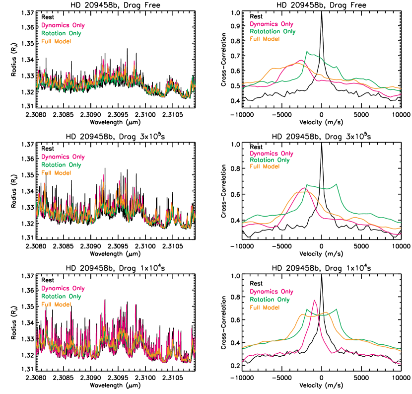
Figure 11.— Left panels: High spectral resolution ($R\sim~{}10^{6}$) planet radius versus wavelength for three models of HD 209458b with various drag strengths. Solid black is the “Rest” model calculated without a Doppler shift. Magenta includes Doppler shifts due to atmospheric dynamics only. Green includes Doppler shifts due to planetary rotation only. In orange, the “Full Model” includes both dynamics and rotation. Right panels: Cross-correlations for the planetary transmission spectra shown at left. As drag becomes stronger one generally finds slower and more peaked wind speeds. See text for additional details.

For each of the three drag cases we calculated the model planet radius vs. wavelength for four variants of the dynamical model. One uses rest-wavelength values (black, this corresponds to a reference case where winds are assumed to be zero), one includes atmospheric dynamics only (magenta, ignoring rotation but using the full 3D winds), one includes only rotation (green, ignoring dynamics), and in orange is the full model, including both dynamics and rotation. The transmission spectra in Figure 11 are somewhat difficult to interpret. Therefore we have also calculated the cross-correlation, compared to the rest wavelength model, across the 1300 wavelengths in our calculation.

There are several aspects of note for these plots. Starting in the upper right of Figure 11, the drag free HD 209458b model, we see that the self cross-correlation is strongly peaked at 0 m s^-1, as expected. The dynamics-only model shows winds that peaked at $-2500\rm\,m\,s^{-1}$ (meaning a blueshift), with strong winds (generally at the equator) reaching beyond $-5000\rm\,m\,s^{-1}$. As seen in the dynamics output, there is also a component of redshift winds, taking up a relatively small fraction of the terminator, which range from $\sim$0 to $5000\rm\,m\,s^{-1}$. Interestingly, for this drag-free case, the cross-correlation curve of the rotation-only model is not symmetric about the zero-velocity point. This asymmetry only appears in models with a strong leading/trailing hemispheric temperature contrast. It appears to be due the trailing (hotter) hemisphere having a larger scale height, and therefore more prominent absorption features. The full model, including dynamics and rotation, has a broader peak than the dynamics-only model due to rotational broadening. The peak $-5000\rm\,m\,s^{-1}$ velocities from dynamics and $-2000\rm\,m\,s^{-1}$, from rotation, lead to velocities on the trailing hemisphere’s equator of $-7000\rm\,m\,s^{-1}$. The full model is not merely just a broadened dynamics-only model due to the asymmetric rotational component.

The weak-drag case (middle right of Figure 11) has a more constrained atmospheric flow, which is generally day-to-night, with a much reduced super-rotating jet. Velocities from dynamics are peaked more narrowly around $-2200\rm\,m\,s^{-1}$ (red curve). The rotational component is close to symmetric, due to the small leading/trailing temperature difference. The full model looks much like the dynamics-only model, broadened due to planetary rotation.

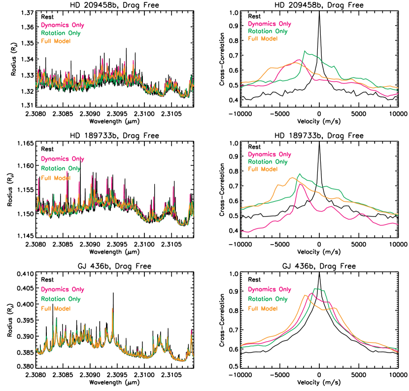
Figure 12.— Left panels: High spectral resolution ($R\sim~{}10^{6}$) planet radius versus wavelength for drag-free models of HD 209458b, HD 189733b, and GJ 436b. Solid black is the “Rest” model calculated without a Doppler shift. Magenta includes Doppler shifts due to atmospheric dynamics only. Green includes Doppler shifts due to planetary rotation only. In orange, the “Full Model” includes both dynamics and rotation. Right panels: Cross-correlations for the planetary transmission spectra shown at left. As the incident flux becomes smaller, from HD 209458b, to HD 189733b, to GJ 436b, peak wind speeds become smaller, and the planet’s dynamics become more dominated by a super-rotating jet. See text for additional details.

The strong-drag case (lower right of Figure 11) has a very constrained circulation, with a relatively uniform day-to-night flow around the entire planet, with little sign of an equatorial jet. The dynamics velocities are strongly peaked at $-1000\rm\,m\,s^{-1}$ and the small leading/trailing temperature contrast leads to a symmetric rotational component. The full model looks very much like a broadened version of the dynamics-only model. The slightly higher peak on the right side of the full model is due to a slight asymmetry in the velocities around $-1000\rm\,m\,s^{-1}$ in the dynamics-only model.

Overall, a comparison of the models in Figure 11 highlights the possibility that the amplitude of drag in the atmosphere of HD 209458b can be inferred from observations. The no-drag, weak-drag, and strong-drag models (Figure 11) exhibit peaks in the cross-correlation centered at $-4$, $-2.5$, and $-1\rm\,km\,s^{-1}$, respectively. We emphasize that these values are the quantitative result of our rigorously calculated transmission spectra from our fully coupled 3D models (and are not, for example, simply the velocity at some assumed pressure of the 3D models). At face value, the results in Figure 11 indicate that models with a drag time constant of $10^{4}$–$10^{6}\rm\,s$ provide a better fit to the Snellen et al. (2010) observations than models with no drag in the upper atmosphere. This is consistent with the inferences drawn in Section 4.3.

The possibility of drag in the atmosphere of HD 209458b is particularly interesting in light of recent suggestions that thermal ionization of alkali metals at high temperature can lead to Lorentz forces that act to brake the atmospheric winds (Perna et al., 2010; Menou, 2012). In the regime of day-to-night flow, air at the terminator has just crossed much of the dayside, and so the wind speed at the terminator is predominantly determined by drag on the dayside rather than the nightside. Secondary-eclipse observations indicate that HD 209458b exhibits a dayside stratosphere with temperatures potentially reaching $\sim$$2000\rm\,K$ (Knutson et al. (2008); see also our Figure 6). Based on the scaling relations in Perna et al. (2010), such high temperatures should lead to very short drag times, potentially consistent with the inferences on drag drawn here.

5.3. Comparing Three Different Planets

Figure 12 allows us to diagnose the different atmospheric dynamics and Doppler shift signatures of HD 209458b, HD 189733b, and GJ 436b. All cases are drag-free. The top row is the same HD 209458b model described in the top row of Figure 11. The dynamical wind velocities for HD 189733b (middle panels of Figure 12) are relatively similar to those of HD 209458b, but lacking a very high velocity component. The planet’s rotation period of 2.2 days is only 63% of the period of HD 209458b, meaning HD 189733b has a significantly larger rotational velocity component. The asymmetry shown is also due to a relatively large leading/trailing temperature contrast. The full model has a smaller, high velocity peak at -5000 m s^-1 due to the strong blue-shifted peak of rotational velocity.

The GJ 436b spectrum clearly shows a transition to a different regime of atmospheric dynamics. The flow is dominated by a wide super-rotating jet, with little flow purely being day to night. This manifests itself in the dynamics-only model as being somewhat symmetric, with a slightly higher cross-correlation peak on the blue-shifted side. The rotational component is nearly symmetric, owning to relative temperature homogenization of the planet. The magnitude of the rotational velocities are quite small because the planet has a small radius. The full model shows little Doppler shift. The spectrum plot at left shows very little difference between all of the models, other than that they have been Doppler broadened compared to the rest model.

6. Discussion

Recent observations suggest that atmospheric winds on hot Jupiters can be directly inferred via the Doppler shift of spectral lines seen during transit (Snellen et al., 2010). Motivated by these observations, we have shown that the atmospheric circulation of hot Jupiters divides into two regimes depending on the strength of the radiative forcing and frictional drag, with implications for the Doppler signature:

• Under moderate stellar fluxes and weak to moderate drag, atmospheric waves generated by the day-night thermal forcing interact with the mean flow to produce fast east-west (zonal) jets. In this regime, air along the terminator flows toward Earth in some regions and away from Earth in others, leading to blue-shifted and red-shifted contributions to the Doppler signature seen during transit. Depending on the speed of the winds relative to the planetary rotation, as well as the variation of zonal winds in latitude and height, this will cause Doppler lines observed during transit to be broadened or, in extreme cases, split into distinct, superposed blue-shifted and red-shifted velocity peaks.

• Under extreme stellar fluxes and/or strong frictional drag, however, the radiative and/or frictional damping is so strong that it damps these waves and inhibits jet formation. At the low pressures sensed by transit measurements, the atmospheric circulation then involves a day-to-night flow, with a return flow at deeper levels. In this regime, the airflow at levels sensed by transit measurements is toward Earth along most or all of the terminator, leading to a predominantly blue-shifted Doppler signature of spectral lines observed during transit.

We presented a theory predicting this regime transition, and we confirmed its existence and explored its properties in one-layer shallow-water models and in three-dimensional models coupling the dynamics to realistic non-gray radiative transfer. We then presented detailed radiative transfer calculations of the transit spectra expected from our 3D models in the 2-$\mu$m spectral region observed by Snellen et al. (2010); these calculations can help to guide future observational efforts.

We also showed that, in the second regime described above, the speed of the day-night windflow depends on the amplitude of the drag at the low pressures sensed by transit measurements. Under relatively weak drag, the wind speeds at the terminator of our HD 209458b models reach $\sim$4–$6\rm\,km\,s^{-1}$ depending on altitude and forcing conditions. Under strong drag, the wind speeds are slower. Interestingly, at the low pressures sensed by transit observations, the drag must be relatively strong—with effective drag time constants of $\sim$$10^{6}\rm\,s$ or less—to reduce the speeds by a significant fraction. Our models of HD 209458b without significant drag in the upper atmosphere produce peak cross-correlations of the transit spectrum corresponding to blueshifts of $\sim$3–$7\rm\,km\,s^{-1}$; this exceeds, albeit marginally, the $\sim$$2\rm\,km\,s^{-1}$ blueshift inferred by Snellen et al. (2010). On the other hand, our models that agree best with the Snellen et al. (2010) inference—where the peak cross-correlations of the transit spectrum lie at $\sim$1–$3\rm\,km\,s^{-1}$—exhibit drag timescales of $10^{4}$–$10^{6}\rm\,s$. This suggests, tentatively, that frictional drag may be important on the dayside of HD 209458b. An attractive possibility is that the dayside of HD 209458b is sufficiently hot for partial ionization to occur, leading to Lorentz-force braking of the winds (Perna et al., 2010; Menou, 2012). Regardless, these models demonstrate that, in principle, measurements of the Doppler shift of spectral lines can place constraints on the amplitude of drag in the atmospheres of hot Jupiters.

In light of this issue, we note that our results differ from those of Miller-Ricci Kempton & Rauscher (2012), who obtained peak cross-correlations in the transmission spectra corresponding to blueshifted velocities of about $-2.5\rm\,km\,s^{-1}$ and $-1\rm\,km\,s^{-1}$ in models without and with drag, respectively. Their velocity shifts for their drag-free case are significantly slower than the velocity shifts we obtain of $-4\rm\,km\,s^{-1}$ for our drag-free HD 209458b model. A significant difference in the two studies is that, in Miller-Ricci Kempton & Rauscher (2012), the heating/cooling in the thermodynamic energy equation was determined using a simplified Newtonian relaxation scheme based on that presented in Cooper & Showman (2005); in contrast, our dynamical models are fully coupled to non-gray radiative transfer, from which the radiative heating/cooling rates are calculated. This may lead to a quantitative difference in the radiative heating rates and hence three-dimensional wind structure. Future work may shed light on the discrepancies between the results.

It is worth mentioning that, within each of the two broad dynamical regimes studied in this paper, there may lie additional subregimes involving important transitions between dynamical mechanisms. For example, in the regime of zonal jets, we have emphasized the development of equatorial superrotation by standing, planetary-scale Rossby and Kelvin waves induced by the day-night thermal forcing (Showman & Polvani, 2011). However, when the stellar flux is lower than considered in most hot-Jupiter models, the importance of the day-night thermal forcing decreases and the equator-to-pole heating gradient becomes dominant. Baroclinic instabilities can then occur, particularly when the rotation rate is fast, and these may lead to multiple mid-latitude east-west jets, with an equatorial jet that may be of either sign depending on the details. A transition analogous to this is evident in models of GJ 436b presented by Lewis et al. (2010). We will explore such dynamical transitions further in future work.

It is also worth discussing the proposal of Montalto et al. (2011), who suggested that the $\sim$$2\rm\,km\,s^{-1}$ blueshift inferred by Snellen et al. (2010) results not from atmospheric winds but from planetary orbital motion due to an eccentric orbit. The radial velocity at the time the planet crosses the line of sight to Earth is ${\rm RV_{0}}=\tilde{K}e\cos\omega/\sqrt{1-e^{2}}$ where $e$ is the eccentricity, $\omega$ is the argument of periastron, and $\tilde{K}\equiv[2\pi G/P]^{1/3}M_{\star}\sin i/(M_{\star}+m_{p})^{2/3}=1.47\times 10^{5}\,\rm m\sec^{-1}$ is a constant, which we have evaluated for HD 209458 parameters. Here, $P$ is the orbital period, $G$ is the gravitational constant, $i$ is the orbital inclination, and $M_{\star}$ and $m_{p}$ are the mass of the star and planet, respectively. Explaining a 2-$\rm km\,\sec^{-1}$ blueshift would thus require that $e\cos\omega\approx 0.014$. Montalto et al. (2011) point out that the eccentricity itself is rather poorly constrained; however, what matters is not eccentricity alone but the combination $e\cos\omega$. A key point, apparently not appreciated by Montalto et al. (2011), is that $e\cos\omega$ is tightly constrained by observations of transit and secondary eclipse. Observations of the relative timing of transit and secondary eclipse from Deming et al. (2005) show that $e\cos\omega<0.002$ at 1-$\sigma$. Observations from Knutson et al. (2008) and Crossfield et al. (2012) place even tighter upper limits on $e\cos\omega$; the latter study yields $e\cos\omega=0.00004\pm 0.00033$, corresponding to a 3-$\sigma$ upper limit of the orbit-induced Doppler shift of $140\rm\,m\,s^{-1}$ at the center of transit. This appears to rule out any orbital explanation for the Doppler shift inferred by Snellen et al. (2010).

One also might wonder whether the Snellen et al. (2010) measurements could be explained by a greater abundance of CO on the eastern terminator, where temperatures are warm and wind preferentially flows from day to night, and a reduced abundance of CO (and enhancement of CH₄) on the western terminator, where temperatures are generally cooler. This is unlikely, however, because the timescales for chemical interconversion between CO and CH₄ in the observable atmosphere are orders of magnitude longer than dynamical timescales, so CO and CH₄ should be chemically quenched (Cooper & Showman, 2006). Therefore, the abundance of CO should be essentially the same everywhere along the terminator at pressures low enough to be sensed remotely.

Finally, while we have emphasized the wind patterns and implications for transit Doppler measurements, the dynamics described here also predict a regime transition in the temperature structure that may be important in explaining thermal observations from light curves and secondary eclipses. The shallow-water models in Figures 3 and 4, and the 3D models in Figure 6, show that the flow tends to a state with small longitudinal temperature variations when radiation and friction are weak, whereas the day-night temperature differences become large when either radiation or friction become strong. Our models therefore predict a transition from small to large fractional day-night temperature differences at the infrared photosphere as stellar flux increases from small to large. We will explore this issue further in future work.

References

- Adcroft et al. (2004) Adcroft, A., Campin, J.-M., Hill, C., & Marshall, J. 2004, Monthly Weather Review, 132, 2845
- Brown (2001) Brown, T. M. 2001, ApJ, 553, 1006
- Burrows et al. (2010) Burrows, A., Rauscher, E., Spiegel, D. S., & Menou, K. 2010, ApJ, 719, 341
- Charbonneau et al. (2005) Charbonneau, D., Allen, L. E., Megeath, S. T., Torres, G., Alonso, R., Brown, T. M., Gilliland, R. L., Latham, D. W., Mandushev, G., O’Donovan, F. T., & Sozzetti, A. 2005, ApJ, 626, 523
- Cho & Polvani (1996) Cho, J. Y.-K., & Polvani, L. M. 1996, Science, 8, 1
- Cooper & Showman (2005) Cooper, C. S., & Showman, A. P. 2005, ApJ, 629, L45
- Cooper & Showman (2006) —. 2006, ApJ, 649, 1048
- Cowan et al. (2007) Cowan, N. B., Agol, E., & Charbonneau, D. 2007, MNRAS, 379, 641
- Crossfield et al. (2010) Crossfield, I. J. M., Hansen, B. M. S., Harrington, J., Cho, J., Deming, D., Menou, K., & Seager, S. 2010, ApJ, 723, 1436
- Crossfield et al. (2012) Crossfield, I. J. M., Knutson, H., Fortney, J., Showman, A. P., Cowan, N. B., & Deming, D. 2012, ApJ, 752, 81
- Deming et al. (2005) Deming, D., Seager, S., Richardson, L. J., & Harrington, J. 2005, Nature, 434, 740
- Dobbs-Dixon et al. (2010) Dobbs-Dixon, I., Cumming, A., & Lin, D. N. C. 2010, ApJ, 710, 1395
- Dobbs-Dixon & Lin (2008) Dobbs-Dixon, I., & Lin, D. N. C. 2008, ApJ, 673, 513
- Dritschel & McIntyre (2008) Dritschel, D. G., & McIntyre, M. E. 2008, Journal of Atmospheric Sciences, 65, 855
- Fortney et al. (2008) Fortney, J. J., Lodders, K., Marley, M. S., & Freedman, R. S. 2008, ApJ, 678, 1419
- Fortney et al. (2010) Fortney, J. J., Shabram, M., Showman, A. P., Lian, Y., Freedman, R. S., Marley, M. S., & Lewis, N. K. 2010, ApJ, 709, 1396
- Fortney et al. (2003) Fortney, J. J., Sudarsky, D., Hubeny, I., Cooper, C. S., Hubbard, W. B., Burrows, A., & Lunine, J. I. 2003, ApJ, 589, 615
- Freedman et al. (2008) Freedman, R. S., Marley, M. S., & Lodders, K. 2008, ApJS, 174, 504
- Hack & Jakob (1992) Hack, J. J., & Jakob, R. 1992, Description of a global shallow water model based on the spectral transform method, Tech. rep., National Center for Atmospheric Research Technical note NCAR/TN-343+STR, Boulder, CO
- Hedelt et al. (2011) Hedelt, P., Alonso, R., Brown, T., Collados Vera, M., Rauer, H., Schleicher, H., Schmidt, W., Schreier, F., & Titz, R. 2011, A&A, 533, A136
- Heng et al. (2011a) Heng, K., Frierson, D. M. W., & Phillipps, P. J. 2011a, MNRAS, 418, 2669
- Heng et al. (2011b) Heng, K., Menou, K., & Phillipps, P. J. 2011b, MNRAS, 413, 2380
- Hubbard et al. (2001) Hubbard, W. B., Fortney, J. J., Lunine, J. I., Burrows, A., Sudarsky, D., & Pinto, P. 2001, ApJ, 560, 413
- Hubeny et al. (2003) Hubeny, I., Burrows, A., & Sudarsky, D. 2003, ApJ, 594, 1011
- Iro et al. (2005) Iro, N., Bézard, B., & Guillot, T. 2005, A&A, 436, 719
- Kataria et al. (2012) Kataria, J. F., Showman, A. P., Lewis, N. K., Fortney, J. J., & Marley, M. S. 2012, ApJ, in preparation
- Knutson et al. (2008) Knutson, H. A., Charbonneau, D., Allen, L. E., Burrows, A., & Megeath, S. T. 2008, ApJ, 673, 526
- Knutson et al. (2007) Knutson, H. A., Charbonneau, D., Allen, L. E., Fortney, J. J., Agol, E., Cowan, N. B., Showman, A. P., Cooper, C. S., & Megeath, S. T. 2007, Nature, 447, 183
- Knutson et al. (2009) Knutson, H. A., Charbonneau, D., Cowan, N. B., Fortney, J. J., Showman, A. P., Agol, E., Henry, G. W., Everett, M. E., & Allen, L. E. 2009, ApJ, 690, 822
- Knutson et al. (2012) Knutson, H. A., Lewis, N., Fortney, J. J., Burrows, A., Showman, A. P., Cowan, N. B., Agol, E., Aigrain, S., Charbonneau, D., Deming, D., Désert, J.-M., Henry, G. W., Langton, J., & Laughlin, G. 2012, ApJ, 754, 22
- Lecavelier Des Etangs et al. (2008) Lecavelier Des Etangs, A., Pont, F., Vidal-Madjar, A., & Sing, D. 2008, A&A, 481, L83
- Lewis et al. (2010) Lewis, N. K., Showman, A. P., Fortney, J. J., Marley, M. S., Freedman, R. S., & Lodders, K. 2010, ApJ, 720, 344
- Li & Goodman (2010) Li, J., & Goodman, J. 2010, ArXiv e-prints
- Lodders (1999) Lodders, K. 1999, ApJ, 519, 793
- Lodders & Fegley (2002) Lodders, K., & Fegley, B. 2002, Icarus, 155, 393
- Lodders & Fegley (2006) Lodders, K., & Fegley, Jr., B. 2006, in Astrophysics Update 2, ed. J. W. Mason (Springer Praxis Books), 1–28
- Madhusudhan & Seager (2011) Madhusudhan, N., & Seager, S. 2011, ApJ, 729, 41
- Marley & McKay (1999) Marley, M. S., & McKay, C. P. 1999, Icarus, 138, 268
- Menou (2012) Menou, K. 2012, ApJ, 745, 138
- Menou & Rauscher (2009) Menou, K., & Rauscher, E. 2009, ApJ, 700, 887
- Menou & Rauscher (2010) —. 2010, ApJ, 713, 1174
- Miller-Ricci Kempton & Rauscher (2012) Miller-Ricci Kempton, E., & Rauscher, E. 2012, ApJ, 751, 117
- Montalto et al. (2011) Montalto, M., Santos, N. C., Boisse, I., Boué, G., Figueira, P., & Sousa, S. 2011, A&A, 528, L17+
- Perna et al. (2012) Perna, R., Heng, K., & Pont, F. 2012, ApJ, 751, 59
- Perna et al. (2010) Perna, R., Menou, K., & Rauscher, E. 2010, ApJ, 719, 1421
- Rauscher & Menou (2010) Rauscher, E., & Menou, K. 2010, ApJ, 714, 1334
- Rauscher & Menou (2012) —. 2012, ApJ, 750, 96
- Rhines (1975) Rhines, P. B. 1975, Journal of Fluid Mechanics, 69, 417
- Rhines (1994) —. 1994, Chaos, 4, 313
- Seager & Sasselov (2000) Seager, S., & Sasselov, D. D. 2000, ApJ, 537, 916
- Shabram et al. (2011) Shabram, M., Fortney, J. J., Greene, T. P., & Freedman, R. S. 2011, ApJ, 727, 65
- Showman et al. (2008) Showman, A. P., Cooper, C. S., Fortney, J. J., & Marley, M. S. 2008, ApJ, 682, 559
- Showman et al. (2009) Showman, A. P., Fortney, J. J., Lian, Y., Marley, M. S., Freedman, R. S., Knutson, H. A., & Charbonneau, D. 2009, ApJ, 699, 564
- Showman & Guillot (2002) Showman, A. P., & Guillot, T. 2002, A&A, 385, 166
- Showman & Polvani (2011) Showman, A. P., & Polvani, L. M. 2011, ApJ, 738, 71
- Showman et al. (2010) Showman, A. P., Y-K. Cho, J., & Menou, K. 2010, ArXiv e-prints
- Snellen et al. (2010) Snellen, I. A. G., de Kok, R. J., de Mooij, E. J. W., & Albrecht, S. 2010, Nature, 465, 1049
- Spiegel et al. (2010) Spiegel, D. S., Burrows, A., Ibgui, L., Hubeny, I., & Milsom, J. A. 2010, ApJ, 709, 149
- Spiegel et al. (2007) Spiegel, D. S., Haiman, Z., & Gaudi, B. S. 2007, ApJ, 669, 1324
- Spiegel et al. (2009) Spiegel, D. S., Menou, K., & Scharf, C. A. 2009, ApJ, 691, 596
- Thrastarson & Cho (2010) Thrastarson, H. T., & Cho, J. 2010, ApJ, 716, 144
- Vallis (2006) Vallis, G. K. 2006, Atmospheric and Oceanic Fluid Dynamics: Fundamentals and Large-Scale Circulation (Cambridge Univ. Press, Cambridge, UK)
- Vallis & Maltrud (1993) Vallis, G. K., & Maltrud, M. E. 1993, J. Phys. Oceanography, 23, 1346
- Vasavada & Showman (2005) Vasavada, A. R., & Showman, A. P. 2005, Reports of Progress in Physics, 68, 1935
- Watkins & Cho (2010) Watkins, C., & Cho, J. 2010, ApJ
- Williams (1978) Williams, G. P. 1978, Journal of Atmospheric Sciences, 35, 1399
- Williams (1979) —. 1979, Journal of Atmospheric Sciences, 36, 932