Exact results on the Kondo-lattice magnetic polaron

Abstract

In this work we revise the theory of one electron in a ferromagnetically saturated local moment system interacting via a Kondo-like exchange interaction. The complete eigenstates for the finite lattice are derived. It is then shown, that parts of these states lose their norm in the limit of an infinite lattice. The correct (scattering) eigenstates are calculated in this limit. The time-dependent Schrödinger equation is solved for arbitrary initial conditions and the connection to the down-electron Green’s function and the scattering states is worked out. A detailed analysis of the down-electron decay dynamics is given.

I introduction

The Kondo-lattice model (KLM) has found widespread application as a basic model for the description of itinerant carriers interacting with local magnetic moments formed by inner shells of the constituting atoms. It was successfully applied in the theoretical description of the europium chalcogenides Methfessel and Mattis (1968); Nolting (1979a); Wachter (1979), aspects of the physics of manganites Salamon and Jaime (2001); Stier and Nolting (2007, 2008); Held and Vollhardt (2000) and the diluted magnetic (III,Mn)V semiconductors Jungwirth et al. (2006); Stier et al. (2011).

It has long been known that the KLM, although it forms a complicated many-body problem not solvable in general, has a non-trivial, exactly solvable limiting case - the (ferro-)magnetic polaronMethfessel and Mattis (1968); Izumov and Medvedev (1971); Richmond (1970). This magnetic polaron is set up by adding one electron into the otherwise empty conduction band and a ferromagnetically saturated background.

Shastry and MattisShastry and Mattis (1981) gave a detailed discussion of the spectral properties of the polaron in terms of the retarded one-electron Green’s function (GF). Berciu and Sawatzky Berciu and Sawatzky (2009) have extended the GF solution to describe complex lattices and longer ranged exchange interactions. Knowledge of the GF allows for the direct calculation of the bare line shape of a photo emission experimentNolting (2009) via the spectral density (SD). This strength of the GF approach comes at the expense of getting only indirect information about the underlying eigenstates of the one-electron quantum system.

Therefore other approaches have solved Schrödinger’s equation directly to get this state informationIzumov and Medvedev (1971); Methfessel and Mattis (1968); Nolting (1979b); Shastry and Mattis (1981). Sigrist et. al.Sigrist et al. (1991) gave a rigorous proof, that the ground state for a system with antiferromagnetic exchange coupling is of incomplete ferromagnetic order. We found these derivations to be incomplete in one way or another and there is, to our knowledge, no exhaustive derivation of the eigenstates for the finite system of $N$ lattice sites in the literature until now.

In the limit $N\to\infty$ the free dispersion of the electron becomes a continuous function of the wavevector. It was van Hove who pointed out in his seminal papers Hove (1955, 1957) that in case of a continuous (free) spectrum the interaction part of the Hamiltonian can lead to persistent effects not amenable to scattering theory. This self-energy effects can be of dissipative nature (finite lifetime of quasi-particles) and/or cloud effects (formation of a new quasi-particle with infinite lifetime). Both effects are present in the problem of the magnetic polaron.

The phenomenon of decaying states has attracted the interest of many physicists. Far from being comprehensive here we just want to mention the works, that have inspired us to the present investigation.

Nakanishi Nakanishi (1958) proposed an extended quantum theory, that contains complex eigenvalues of the Hamiltonian which can be associated with an unstable particle. To this aim he constructed the analytic continuation of the propagator for that particle and found poles in the continuation. By introducing a complex distribution he was able to construct a new eigenstate of the Hamiltonian with complex eigenvalue (equal to the pole position) leading to an exponential decay of the particle in time. Deviations from an exponential decay law at long times and the importance of the van Hove singularity on the lower bound of the spectrum was discussed by HöhlerHöhler (1958) and KhalfinKhalfin (1958). The short-time deviations and the resulting quantum Zeno effect where derived in Misra and Sudarshan (1977); Chiu et al. (1977). Sudarshan et. al. have extended the ideas of NakanishiSudarshan et al. (1978) and gave also a more formal derivation in a rigged Hilbert space formalismParravicini et al. (1980); Sudarshan and Chiu (1993).

We will use the methods developed in the above mentioned works as a pragmatic device to get a deeper understanding of the decay dynamics of a down-electron in the problem of the magnetic polaron.

The paper is organized as follows.
In section II we explain the model Hamiltonian and give the parameters used throughout this work. Section III summarizes the results obtained with the GF approach. The spectral density of up/down-electrons is discussed in detail. The complete eigenstates for the finite lattice are derived in section IV. Section V is devoted to the problems arising in the limit of an infinite lattice. New (scattering) eigenstates are constructed and the time-dependent Schrödinger equation is solved for arbitrary initial conditions. The connection of certain initial conditions with the electronic GF is given. In section VI a detailed analysis of the dynamics of the quantum system for two different initial conditions is given. The connection to the scattering states and the limitations of scattering theory are discussed. Finally we give a summary and draw conclusions in section VII.

II model

Throughout the paper we are concerned with the s-f-like Hamiltonian:

$$H=\sum_{ij\sigma}T_{ij}c_{i\sigma}^{+}c_{j\sigma}-\frac{J}{2}\sum_{i\sigma}\left(z_{\sigma}S^{z}_{i}c_{i\sigma}^{+}c_{i\sigma}+S^{\sigma}_{i}c_{i-\sigma}^{+}c_{i\sigma}\right)$$ (1)

where $\sigma=\pm$, $z_{\pm}=\pm 1$ and $S^{\pm}_{i}=S^{x}_{i}\pm iS^{y}_{i}$, describing free electrons hopping trough the lattice and undergoing a local (contact) interaction with immobile local moments formed by the inner shells of the underlying atoms. The $c_{i\sigma}^{+}$ ($c_{i\sigma}$) denote the creation (annihilation) operator of an electron with spin $\sigma$ at lattice site $\mathbf{R}_{i}$.
The above Hamiltonian constitutes a highly involved many-body problem not solvable for the general case. It has long been known, however, that there exists a non-trivial solution in the limiting case of one electron in the otherwise empty conduction band moving in a lattice of fully ferromagnetically ordered background spins ($T=0K$).
The Hamiltonian (1) does not distinguish energetically between different configurations of the localized spins in case of an empty band. One could enforce a fully aligned ground state by introducing an additional direct exchange term of Heisenberg type between the localized spins as was done in some works Shastry and Mattis (1981). This additional term would lead to a true magnon dispersion of the localized moments (which is flat in our case) and to energy corrections of the eigenstates where a magnon is present. Since these energy corrections are small (typical magnon energies are 2-3 orders of magnitude smaller than the electronic energies) and the additional term would complicate the already involved calculations we omit this term and choose the fully aligned state out of the highly degenerate ground-state manifold “by hand”. One has to keep in mind, however, that the dynamics of the localized spins are mediated only by the electron.
If not stated otherwise we will use the following model-parameters for the concrete evaluation of our theory. We choose a magnetic moment $S=\frac{7}{2}$ for the local spin system which reflects the magnetic moment of the prototypical rare-earth compounds EuO and EuS. The underlying lattice will be the three-dimensional (3D) simple cubic (SC) lattice and the hopping $T_{ij}$ is chosen to give the tight-binding dispersion:

$$\epsilon_{\mathbf{k}}=-\frac{W}{6}\left(\cos(kx)+\cos(ky)+\cos(kz)\right)$$ (2)

with bandwidth $W=1$.

III one-electron green’s function

Figure 1: (color online) Down electron spectral density along lines of high symmetry in $\mathbf{k}$-space and quasi-particle density of states for two different coupling strengths $J$. Parameters: $S=3.5$, $W=1.0$ eV.

The limiting case of the “magnetic polaron” is usually discussed in terms of the retarded one-electron Green’s function (GF). For the derivation of the latter one transforms (1) into reciprocal $\mathbf{k}$-space and writes down the equation of motion (EQM) of the GF. Under the above assumptions (ferromagnetic saturated local moment system, empty band) this EQM can be simplified in case of an up-electron (parallel to local moments) to give:

$$G_{\mathbf{k}\uparrow}(E)=G^{(0)}_{\mathbf{k}}(E+\frac{JS}{2})=\frac{1}{E+i0^{+}-\epsilon_{\mathbf{k}}+\frac{JS}{2}}.$$ (3)

An up-electron behaves essentially like a free electron with a shifted energy equal to the mean field value due to the ferromagnetic background. It has an infinite lifetime because it will not find a partner to flip its spin in the already saturated local moment system.
The situation is quite different for a down-electron. In the EQM appears a higher spin-flip GF (SF-GF) and one has to go one step further in the EQM-hierarchy to get a closed set of equations. This results in:

$$G_{\mathbf{k}\downarrow}(E)=\frac{1}{E+i0^{+}-\epsilon_{\mathbf{k}}-\Sigma_{\downarrow}(E)},$$ (4)

with the electronic self-energyShastry and Mattis (1981):

$$\Sigma_{\downarrow}(E)=\frac{JS}{2}\left(1+\frac{JG^{(0)}(E+\frac{JS}{2})}{1-\frac{J}{2}G^{(0)}(E+\frac{JS}{2})}\right),$$ (5)

where $G^{(0)}(E)=\frac{1}{N}\sum_{\mathbf{k}}G^{(0)}_{\mathbf{k}}(E)$ denotes the $\mathbf{k}$-summed free electronic GF. The center of gravity of the down-spectral density is given by the first spectral moment:

$$M_{\mathbf{k}\downarrow}^{(1)}=\epsilon_{\mathbf{k}}+\frac{JS}{2},$$ (6)

which is the mean-field energy of the down-electron. Despite this one expects significant changes in the down-spectral density compared to the mean-field result due to correlation effects. Especially possible spin-flips of the down-electron should result in a finite lifetime of quasi-particles as is indicated by the complex-valued self-energy. Inspecting (5) reveals, that states with finite lifetime can be expected exactly in the energy range of the up-spectrum because the self-energy has a finite imaginary part there. These states are commonly called the scattering states. In order to fulfill (6) for the center of gravity one then should find additional states (of infinite lifetime) above ($J>0$) or below ($J<0$) the scattering states as real roots of the denominator of (4) at least for sufficiently large $J$. In the next section we will show, that there is exactly one such additional state called the bound state or polaron state.
To illustrate our findings we have plotted the down-spectral density and the quasi-particle density of states (QDOS) in Fig. 1 for two different values of $J$. For large enough $J$ ($J=0.3$ eV, upper figure) the bound states are completely separated from the scattering states and form a polaron band. It can be shown Richmond (1970); Izumov and Medvedev (1971), that in the limit of large $J$ ($|J|\gg W/S$) this polaron band has its center of gravity at $E_{c}^{p}=\frac{J}{2}(S+1)$ and the bandwidth is reduced by a factor of $\frac{2S}{2S+1}$ compared to $W$.
When $J$ is smaller ($J=0.1$ eV, lower figure) parts of the polaron-band dip into the scattering states. There is still a visible polaron dispersion in the scattering region, but now in form of a peak with finite linewidth implying a finite lifetime of the quasi-particle. We will show in a later section (VI), that each quasi-particle peak in the scattering states is associated with a pole in the suitably analytically continued propagator leading to an exponential contribution in the decay dynamics. The polaron dispersion is strongly disturbed at the positions of the van Hove singularities (horizontal dashed lines) of the scattering spectrum. The special role of the van Hove singularities as limit/branch points for analytic continuation will also become clear in that section.

IV The finite system - Eigenstates

In this section we derive the complete eigensystem for a finite lattice ($N$ lattice sites) with periodic boundary conditions. Although parts of this derivation can be found in the literature Methfessel and Mattis (1968); Shastry and Mattis (1981), to our knowledge, the complete spectrum was never calculated. Especially the appearance of pure up-electron states with one magnon emitted is not recognized.
We use the following notation. The state of one electron with wavevector $\mathbf{k}$, spin $\sigma$ and all local moments aligned (magnon vacuum) will be denoted by:

$$c_{\mathbf{k}\sigma}^{+}|0;0\rangle=|\mathbf{k}\sigma;0\rangle.$$ (7)

An up-electron with wavevector $\mathbf{k}$ plus a magnon of wavevector $\mathbf{q}$ is written as:

$$\frac{1}{\sqrt{2S}}S_{\mathbf{q}}^{-}c_{\mathbf{k}\uparrow}^{+}|0;0\rangle=|\mathbf{k}\uparrow;\mathbf{q}\rangle.$$ (8)

These states span the Hilbert subspace we are interested in. The Hamiltonian (1) commutes with the z-component of the total spin operator $\hat{S}_{tot}^{z}=\sum_{i}(S_{i}^{z}+\frac{1}{2}\sum_{\sigma}z_{\sigma}\hat{n}_{i\sigma})$. Therefore we can classify the eigenstates by $S_{tot}^{z}$ and by their (outer) wavevector $\mathbf{k}$ due to translational invariance.
In the subspace of $S_{tot}^{z}=NS+\frac{1}{2}$ the eigenstates are simply the up-electron states with magnon vacuum:

$$H|\mathbf{k}\uparrow;0\rangle=\left(\epsilon_{\mathbf{k}}-\frac{JS}{2}\right)|\mathbf{k}\uparrow;0\rangle.$$ (9)

The subspace $S_{tot}^{z}=NS-\frac{1}{2}$ is more interesting. It will be spanned by the states of one down electron in magnon vacuum and an up-electron plus one magnon emitted. By using the following Ansatz for the wave-function:

$$|\Psi_{\mathbf{k}}^{n}\rangle=A\left\{\alpha_{\mathbf{k}}|\mathbf{k}\downarrow;0\rangle+\sum_{\mathbf{q}}\beta_{\mathbf{k,q}}|\mathbf{k-q}\uparrow;\mathbf{q}\rangle\right\}$$ (10)

we get a system of equations for the coefficients from Schrödinger’s equation:

$$0 = \left(E-\epsilon_{\mathbf{k}}-\frac{JS}{2}\right)\alpha_{\mathbf{k}}+J\sqrt{\frac{S}{2N}}\sum_{\mathbf{q}}\beta_{\mathbf{k,q}}$$ (11)

$$0 = \left(E-\epsilon_{\mathbf{k-q}}+\frac{JS}{2}\right)\beta_{\mathbf{k,q}}+J\sqrt{\frac{S}{2N}}\alpha_{\mathbf{k}}-\frac{J}{2N}\sum_{\mathbf{q}}\beta_{\mathbf{k,q}}.$$

This are $N+1$ equations for the same number of coefficients and we expect $N+1$ eigenvalues per $\mathbf{k}$-value ($N(N+1)$ eigenvalues in total). The characteristic polynomial of (11) turns out to be of the simple form:

$$0=\left(\prod_{i=1}^{N}E_{i}\right)\left(E_{0}-\frac{J}{2}(E_{0}+JS)\frac{1}{N}\sum_{j}^{N}\frac{1}{E_{j}}\right)$$ (12)

with

$$E_{0} = E-\epsilon_{\mathbf{k}}-\frac{JS}{2},$$ (13)

$$E_{n\neq 0} = E-\epsilon_{\mathbf{k-q_{n}}}+\frac{JS}{2}.$$ (14)

Not all $\epsilon_{\mathbf{k-q_{n}}}$ will be different by symmetry arguments. Therefore we collect all equal $\epsilon_{\mathbf{k-q_{n}}}$ in groups, where the numeric value of the group members is denoted by $\epsilon_{\mathbf{k}}^{(n)}$ with the convention that $\epsilon_{\mathbf{k}}^{(1)}=\epsilon_{\mathbf{k}}$. Let us assume that $N_{G}$ such groups with respective degree of degeneracy $g_{n}$ exist. The $\mathbf{q}$ belonging to one group are denoted by $\mathbf{q}_{l}^{(n)}$ with $l\in 0\cdots g_{n}-1$. With the definition: $F_{n}=E-\epsilon_{\mathbf{k}}^{(n)}+\frac{JS}{2}$ we can recast (12) to give:

$$0=\left(\prod_{i=1}^{N_{G}}F_{i}^{g_{i}}\right)\left(E_{0}-F_{1}\frac{J}{2N}\sum_{j=1}^{N_{G}}\frac{g_{j}}{F_{j}}\right).$$ (15)

The first product contributes $N_{G}$ differing eigenvalues:

$$E_{\mathbf{k}}^{(n)}=\epsilon_{\mathbf{k}}^{(n)}-\frac{JS}{2}.$$ (16)

The respective multiplicity of these eigenvalues will be $g_{n}-1$, since we divide by $F_{j}$ (for $j>1$) in the second factor of (15). Only $E_{\mathbf{k}}^{(1)}$ has the full multiplicity $g_{1}$. For the construction of the eigenvectors we notice first, that the eigenenergies (16) are equal to the pure up-electron energies (9) found in the $S_{tot}^{z}=NS+\frac{1}{2}$ sector of the Hilbert space. It is therefore reasonable to assume the sought-after states to be up-states as well. We try $\alpha_{\mathbf{k}}=0$ and $\beta_{\mathbf{k,q}}\neq 0$ only for $\mathbf{q}\in\{\mathbf{q}^{(n)}_{l}\}$ in our Ansatz (10). From (11) we then get the condition:

$$\sum_{\mathbf{q}\in\{\mathbf{q}^{(n)}_{l}\}}\beta_{\mathbf{k,q}}=0.$$ (17)

This condition can be nontrivial fulfilled when the $\beta_{\mathbf{k,q}}$ are chosen to be suitable normalized powers of the primitive $g_{n}$th roots of unity. With this we find for the eigenstates:

$$|\Psi_{\mathbf{k}}^{n,m}\rangle=\frac{1}{\sqrt{g_{n}}}\sum_{l=0}^{g_{n}-1}\mathrm{e}^{i\frac{2\pi}{g_{n}}ml}|\mathbf{k-q}_{l}^{(n)}\uparrow;\mathbf{q}_{l}^{(n)}\rangle$$ (18)

where $m\in 1\cdots g_{n}-1$ is numerating the eigenstates of the subspace with energy $E_{\mathbf{k}}^{(n)}$.
One eigenstate is missing so far, since the degeneracy of $E_{\mathbf{k}}^{(1)}$ is $g_{1}$. The states, which have only an up-electron (plus magnon) component are exhausted by (18). By substituting $E_{\mathbf{k}}^{(1)}$ into (11) a simple calculation shows, that the last eigenstate is given by:

$$|\Psi_{\mathbf{k}}^{1,0}\rangle=\frac{|\mathbf{k}\downarrow;0\rangle+\frac{\sqrt{2NS}}{g_{1}}\sum_{l=0}^{g_{1}-1}|\mathbf{k-q}_{l}^{(1)}\uparrow;\mathbf{q}_{l}^{(1)}\rangle}{\sqrt{1+\frac{2NS}{g_{1}}}}.$$ (19)

It has a finite down-electron component.
Until now we have found $1+\sum_{i=1}^{N_{G}}(g_{i}-1)=1+N-N_{G}$ eigenvalues and corresponding eigenvectors from the first factor of (15). The remaining $N_{G}$ eigenvalues come from the second factor:

$$0 = E_{0}-F_{1}\frac{J}{2N}\sum_{j=1}^{N_{G}}\frac{g_{j}}{F_{j}}$$

$$= E-\epsilon_{\mathbf{k}}-\frac{J}{2}\left(S+1+\frac{1}{N}\sum_{n=2}^{N_{G}}\frac{g_{n}(\epsilon_{\mathbf{k}}^{(n)}-\epsilon_{\mathbf{k}})}{E-\epsilon_{\mathbf{k}}^{(n)}+\frac{JS}{2}}\right).$$

The function on the rhs of (IV) has $N_{G}-1$ zero-crossings between the up-state energies (16) and one above ($J>0$) or below ($J<0$) the scattering states near $E_{c}\approx\epsilon_{\mathbf{k}}+\frac{J}{2}(S+1)$.

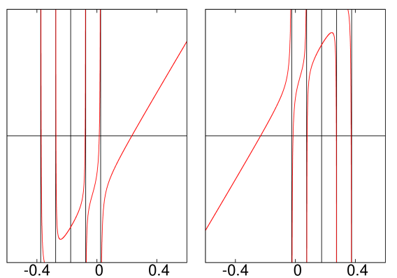
Figure 2: (color online) Plot of eigenvalue equation (IV) with positive (left figure) and negative (right figure) $J$. Parameters: $|J|=0.1$, $S=3.5$, $\epsilon_{\mathbf{k}}=0$, $\epsilon_{\mathbf{k}}^{(1)}=-0.2$, $\epsilon_{\mathbf{k}}^{(2)}=-0.1$, $\epsilon_{\mathbf{k}}^{(3)}=0.1$, $\epsilon_{\mathbf{k}}^{(4)}=0.2$, $g_{n}=1$.

The situation is depicted in Fig. 2. Rewriting (IV) we get an implicit equation for the (polaron)-eigenenergies:

$$E_{\mathbf{k}}^{p,(n)}=\epsilon_{\mathbf{k}}+\frac{J}{2}\left(S+1+\Phi_{\mathbf{k}}(E_{\mathbf{k}}^{p,(n)}+\frac{JS}{2})\right)$$ (21)

with

$$\Phi_{\mathbf{k}}(z)=\frac{1}{N}\sum_{\mathbf{q}}\frac{\epsilon_{\mathbf{k-q}}-\epsilon_{\mathbf{k}}}{z-\epsilon_{\mathbf{k-q}}}.$$ (22)

The corresponding eigenstates are again obtained from (11) to yield:

$$|\Psi_{\mathbf{k}}^{p,(n)}\rangle = \mathcal{N}|\mathbf{k}\downarrow;0\rangle$$

$$- \mathcal{N}\frac{\sum_{\mathbf{q}}\left(1+\frac{\epsilon_{\mathbf{k-q}}-\epsilon_{\mathbf{k}}}{E_{\mathbf{k}}^{p,(n)}-\epsilon_{\mathbf{k-q}}+\frac{JS}{2}}\right)|\mathbf{k-q}\uparrow;\mathbf{q}\rangle}{\sqrt{2NS}}$$

with the obvious normalization factor:

$$\mathcal{N}=\left(1+\frac{1}{2NS}\sum_{\mathbf{q}}\left|1+\frac{\epsilon_{\mathbf{k-q}}-\epsilon_{\mathbf{k}}}{E_{\mathbf{k}}^{p,(n)}-\epsilon_{\mathbf{k-q}}+\frac{JS}{2}}\right|^{2}\right)^{-\frac{1}{2}}.$$ (24)

V The infinite system

In the limit of an infinite lattice ($N\to\infty$) the free electronic band energies $\epsilon_{\mathbf{k}}$ become continuous functions of the wavevector. All summations will therefore be replaced by integrations:

$$\frac{1}{N}\sum_{\mathbf{k}}\rightarrow\frac{1}{V_{\mathrm{BZ}}}\int\mathrm{d}\mathbf{k}.$$ (25)

In this limit all eigenstates with down-electron part whose energies lie in the scattering region ($\epsilon_{\mathbf{k}}^{\mathrm{min}}-\frac{JS}{2}\leq E\leq\epsilon_{\mathbf{k}}^{\mathrm{max}}-\frac{JS}{2}$) lose their norm as becomes clear immediately by inspecting (19) and (24). Only the bound (polaron) state above ($J>0$) or below ($J<0$) the scattering region will survive provided that $J$ is sufficiently large so that the state is energetically well separated from the scattering states.
The question then becomes, what are the eigenstates in this limit? We will construct scattering states and show, that these states (+ polaron state) form a complete basis in the continuum limit. Thereafter we solve the time-dependent Schrödinger equation which does not suffer from such difficulties for arbitrary initial conditions and show the connection to Green’s function theory and the scattering states.

V.1 scattering states

In this section we ask for the result of a scattering process of an up-electron with a magnon, that is we want to solve the Lippmann-Schwinger equation Lippmann and Schwinger (1950) :

$$|\mathbf{k-q}\uparrow;\mathbf{q}\rangle^{\pm}=|\mathbf{k-q}\uparrow;\mathbf{q}\rangle+R_{\pm}H_{1}|\mathbf{k-q}\uparrow;\mathbf{q}\rangle^{\pm},$$ (26)

with the free propagator $R_{\pm}=(E_{0}-H_{0}\pm i0^{+})^{-1}$. First we divide the Hamiltonian (1) into a free part $H_{0}$ and an interaction part $H_{1}$:

$$H_{0} = \sum_{\mathbf{k}\sigma}\left(\epsilon_{\mathbf{k}}-z_{\sigma}\frac{JS}{2}\right)\hat{n}_{\mathbf{k}\sigma},$$ (27)

$$H_{1} = -\frac{J}{2\sqrt{N}}\sum_{\mathbf{kq}\sigma}\left(z_{\sigma}S_{\mathbf{q}}^{z}c_{\mathbf{k-q}-\sigma}^{+}c_{\mathbf{k}\sigma}+S_{\mathbf{q}}^{\sigma}c_{\mathbf{k-q}-\sigma}^{+}c_{\mathbf{k}\sigma}\right)$$

$$+ \sum_{\mathbf{k}\sigma}z_{\sigma}\frac{JS}{2}\hat{n}_{\mathbf{k}\sigma}.$$

With this division one can derive:

$$R_{\pm}H_{1}|\mathbf{k-q}\uparrow,\mathbf{q}\rangle = |Z_{1}\rangle+|Z_{2}\rangle$$

$$R_{\pm}H_{1}|Z_{1}\rangle = A_{1}|Z_{2}\rangle,$$

$$R_{\pm}H_{1}|Z_{2}\rangle = A_{2}(|Z_{1}\rangle+|Z_{2}\rangle),$$ (28)

where the $A_{i}$ and $|Z_{i}\rangle$ are given in the appendix (53). Defining the matrix:

$$\hat{\mathbf{A}}=\begin{pmatrix}0&A_{1}\\ A_{2}&A_{2}\end{pmatrix}=\hat{\mathbf{U}}\hat{\mathbf{D}}\hat{\mathbf{U}}^{-1},$$ (29)

we can iterate (26) and get:

$$|\mathbf{k}-\mathbf{q}\uparrow\rangle^{\pm} =|\mathbf{k}-\mathbf{q}\uparrow\rangle+\begin{pmatrix}1\\ 1\end{pmatrix}\left(\sum_{l=0}^{\infty}\hat{\mathbf{A}}^{l}\right)\begin{pmatrix}|Z_{1}\rangle\\ |Z_{2}\rangle\end{pmatrix}$$

$$=|\mathbf{k}-\mathbf{q}\uparrow\rangle+\begin{pmatrix}1\\ 1\end{pmatrix}\hat{\mathbf{U}}\left(\sum_{l=0}^{\infty}\hat{\mathbf{D}}^{l}\right)\hat{\mathbf{U}}^{-1}\begin{pmatrix}|Z_{1}\rangle\\ |Z_{2}\rangle\end{pmatrix}$$

$$=|\mathbf{k}-\mathbf{q}\uparrow\rangle+\frac{|Z_{1}\rangle}{1-A_{2}(1+A_{1})}+\frac{|Z_{2}\rangle}{\frac{1}{1+A_{1}}-A_{2}}$$

$$=\alpha_{\mathbf{q}}^{\mathbf{k}}|\mathbf{k}\downarrow;0\rangle+\sum_{\mathbf{q^{\prime}}}\beta_{\mathbf{q},\mathbf{q^{\prime}}}^{\mathbf{k}}|\mathbf{k}-\mathbf{q^{\prime}}\uparrow;\mathbf{q^{\prime}}\rangle$$ (30)

for the ingoing and outgoing scattering states. The diagonal matrix $\hat{\mathbf{D}}$ and the matrix of the eigenvectors $\hat{\mathbf{U}}$ are given in the appendix A as equation (55), the coefficients $\alpha_{\mathbf{q}}^{\mathbf{k}}$ and $\beta_{\mathbf{q},\mathbf{q^{\prime}}}^{\mathbf{k}}$ as equation (56).
It remains to show, that the so constructed scattering states form a basis set in the limit of an infinite lattice. Applying the Hamiltonian results in:

$$H|\mathbf{k}-\mathbf{q}\uparrow;\mathbf{q}\rangle^{\pm} = \left(\epsilon_{\mathbf{k-q}}-\frac{JS}{2}\right)|\mathbf{k}-\mathbf{q}\uparrow;\mathbf{q}\rangle^{\pm}$$

$$+ \sum_{\mathbf{q^{\prime}}}\mathcal{R}_{\mathbf{q,q^{\prime}}}^{\mathbf{k}}|\mathbf{k}-\mathbf{q^{\prime}}\uparrow;\mathbf{q^{\prime}}\rangle.$$

The residue term $\mathcal{R}_{\mathbf{q,q^{\prime}}}^{\mathbf{k}}$ that is given in the appendix (57) goes to zero as $O(1/N)$. Therefore the scattering states (30) indeed become the correct eigenstates in the infinite lattice limit with densely lying eigenenergies in the expected region.

V.2 time dependent Schrödinger equation

Choosing the Ansatz:

$$|\Psi_{\mathbf{k}}(t)\rangle=\alpha_{\mathbf{k}}(t)|\mathbf{k}\downarrow;0\rangle+\sum_{\mathbf{q}}\beta_{\mathbf{k,q}}(t)|\mathbf{k-q}\uparrow;\mathbf{q}\rangle$$ (32)

for the wave-function one gets the following system of differential equations from the time-dependent Schrödinger equation ($\hbar=1$):

$$i\dot{\alpha}_{\mathbf{k}}(t) = \left(\epsilon_{\mathbf{k}}+\frac{JS}{2}\right)\alpha_{\mathbf{k}}(t)-J\sqrt{\frac{S}{2N}}\sum_{\mathbf{q}}\beta_{\mathbf{k,q}}(t),$$

$$i\dot{\beta}_{\mathbf{k,q}}(t) = \left(\epsilon_{\mathbf{k-q}}-\frac{JS}{2}\right)\beta_{\mathbf{k,q}}(t)-J\sqrt{\frac{S}{2N}}\alpha_{\mathbf{k}}(t)$$ (33)

$$+\frac{J}{2N}\sum_{\mathbf{q}}\beta_{\mathbf{k,q}}(t).$$

This can be transformed into a system of algebraic equations by the Laplace transform:

$$\bar{f}(s)=\int_{0}^{\infty}\mathrm{e}^{-st}f(t)\mathrm{d}t;\>\mathrm{Re}(s)>0$$ (34)

and one obtains the solution for the coefficients in the $s$-domain:

$$\bar{\alpha}_{\mathbf{k}}(s) = \frac{i\alpha_{\mathbf{k}}(0)}{is-\epsilon_{\mathbf{k}}-\frac{JS}{2}\left(1+\frac{JG^{(0)}(is+\frac{JS}{2})}{1-\frac{J}{2}G^{(0)}(is+\frac{JS}{2})}\right)}$$

$$- \frac{iJS}{\sqrt{2NS}}\sum_{\mathbf{q}}\frac{\beta_{\mathbf{k,q}}(0)}{\left(is-\epsilon_{\mathbf{k-q}}+\frac{JS}{2}\right)h_{1}(is)},$$

$$\bar{\beta}_{\mathbf{k,q}}(s) = \frac{i\beta_{\mathbf{k,q}}(0)+\frac{i\alpha_{\mathbf{k}}(0)-(is-\epsilon_{\mathbf{k}}+\frac{JS}{2})\bar{\alpha}_{\mathbf{k}}(s)}{\sqrt{2NS}}}{is-\epsilon_{\mathbf{k-q}}+\frac{JS}{2}},$$ (36)

with

$$h_{1}(z)=z-\epsilon_{\mathbf{k}}-\frac{J}{2}\left(S+1+\Phi_{\mathbf{k}}(z+\frac{JS}{2})\right).$$ (37)

For the back-transformation into the time-domain one has to solve the Bromwich integral:

$$f(t)=\frac{1}{2\pi i}\int_{\gamma-i\infty}^{\gamma+i\infty}\mathrm{e}^{st}\bar{f}(s)\mathrm{d}s,$$ (38)

where $\gamma$ is a real constant, that is larger than the real part of any singularity of $\bar{f}(s)$. In our case all singularities/branch cuts of $\bar{\alpha}_{\mathbf{k}}(s)$ and $\bar{\beta}_{\mathbf{k,q}}(s)$ lie in a finite domain on the imaginary axis. Therefore $\gamma$ can take any value $\gamma>0$.

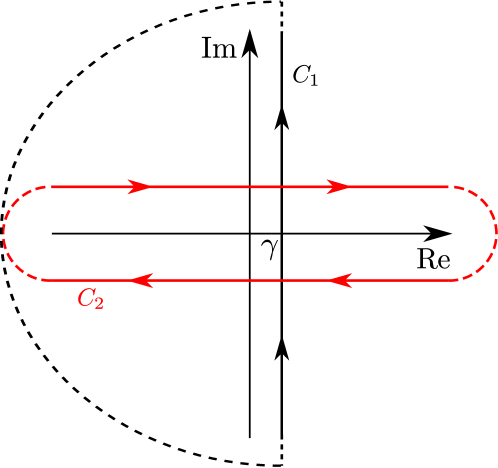
Figure 3: (color online) Integration contour in complex plane.

The integration path is shown in Fig. 3 and denoted by $C_{1}$. The contour can be closed at infinity since the integrand vanishes there (dashed black line). Performing the variable substitution $s\to-iz$ and a contour deformation one can change the integration path to become $C_{2}$ (red line). The singularities/ branch cuts now lie on the real axis.
We will give the solutions for two special boundary conditions here. The choice:

$$\mathrm{a)}\;\alpha_{\mathbf{k}}(t=0)=1;\beta_{\mathbf{k,q}}(t=0)=0,\forall\mathbf{q}$$ (39)

results in:

$$\alpha_{\mathbf{k}}(t) =\frac{-1}{2\pi i}\int_{C_{2}}\mathrm{d}z\frac{\mathrm{e}^{-izt}}{z-\epsilon_{\mathbf{k}}-\frac{JS}{2}\left(1+\frac{JG^{(0)}(z+\frac{JS}{2})}{1-\frac{J}{2}G^{(0)}(z+\frac{JS}{2})}\right)}$$

$$=\frac{-1}{2\pi i}\int_{-\infty}^{\infty}\mathrm{d}x\>\mathrm{e}^{-ixt}\left(G_{\mathbf{k}\downarrow}(x+i0^{+})-G_{\mathbf{k}\downarrow}(x-i0^{+})\right)$$

$$=\int_{-\infty}^{\infty}\mathrm{d}x\>\mathrm{e}^{-ixt}S_{\mathbf{k}\downarrow}(x),$$ (40)

that is, $\alpha_{\mathbf{k}}(t)$ is the Fourier transform of the spectral density obtained from the down-electron Green’s function derived earlier (4).
Choosing:

$$\mathrm{b)}\;\beta_{\mathbf{k,q_{n}}}(0)=1;\alpha_{\mathbf{k}}(0)=\beta_{\mathbf{k,q_{m}}}(0)=0,\forall m\neq n$$ (41)

one gets:

$$\alpha_{\mathbf{k}}(t)=\frac{JS}{\sqrt{2NS}}\frac{1}{2\pi i}\int_{C_{2}}\mathrm{d}z\>\frac{\mathrm{e}^{-izt}}{\left(z-\epsilon_{\mathbf{k-q_{n}}}+\frac{JS}{2}\right)h_{1}(z)}.$$ (42)

It is to be expected, that this will become the $\alpha_{\mathbf{q}_{n}}^{\mathbf{k}}$ of the scattering states (30) for large times. We will test this conjecture in the next section, when we have build up the machinery to investigate different time domains of $\alpha_{\mathbf{k}}(t)$.

VI dynamics of decay

The absolute square of the coefficient $\alpha_{\mathbf{k}}(t)$ in (32) can be interpreted as the probability to find a down-electron in the system at time $t$. In Fig. 4 we show $P(t)=|\alpha_{\mathbf{k}}(t)|^{2}$ of a system subjected to the boundary conditions (39) for two different couplings $J=0.1/0.3$ eV.

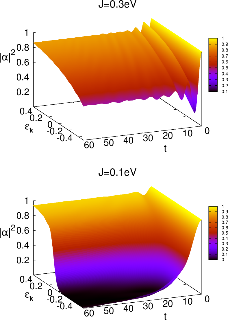
Figure 4: (color online) Probability to find a down-electron $P(t)=|\alpha_{\mathbf{k}}(t)|^{2}$ as a function of time and the free electron dispersion $\epsilon_{\mathbf{k}}$ for two different values of $J$. The time is given in units of $\approx 6.58212*10^{-16}$s. Parameters: $S=3.5$, $W=1.0$ eV.

For large $J$ (upper panel in Fig. 1 shows the corresponding spectral density) there is always a finite probability to find a down-electron in the system. $P(t)$ shows characteristic oscillations over time. These oscillation will be damped with increasing $t$ and $P(t)$ becomes static in the long-run limit. When $J$ is smaller, parts of the polaron band dip into the scattering states (lower panel in Fig. 1). For wavevectors $\mathbf{k}$ where $\epsilon_{\mathbf{k}}$ lies below a certain threshold $P(t)$ decreases exponentially and become zero in the long-run limit. The down-electron decays inevitably. However, it is clearly visible in the figure, that there are deviations from an exponential decay law in the short and the long time regime. We will now give a more detailed analysis of the different time domains.

VI.1 short time behavior

For small times a Taylor expansion of the exponential function in (V.2) gives:

$$\alpha_{\mathbf{k}}(t) = \int\limits_{-\infty}^{\infty}\mathrm{d}xS_{\mathbf{k}\downarrow}(x)\left[1+ixt-\frac{(xt)^{2}}{2}-i\frac{(xt)^{3}}{6}+\cdots\right]$$ (43)

$$= 1+iM_{\mathbf{k}\downarrow}^{(1)}t-\frac{M_{\mathbf{k}\downarrow}^{(2)}}{2}t^{2}-i\frac{M_{\mathbf{k}\downarrow}^{(3)}}{6}t^{3}+O(t^{4}).$$

The spectral moments $M_{\mathbf{k}\downarrow}^{(i)}$ can be calculated exactly in our case and we give the first four in the appendix (C). From this we get the short time expansion of $P(t)$:

$$|\alpha_{\mathbf{k}}(t)|^{2}=1-C_{1}t^{2}+O(t^{4})$$ (44)

with

$$C_{1}=M_{\mathbf{k}\downarrow}^{(2)}-(M_{\mathbf{k}\downarrow}^{(1)})^{2}=\frac{J^{2}S}{2}.$$ (45)

Since $C_{1}\geq 0$ $P(t)$ will always decrease (or stay constant) for small times as it should be for normalization reasons. The change of $P(t)$ has a zero slope at $t=0$ since $\mathrm{d}P(t)/\mathrm{d}t|_{0}=0$. This leads to the famous quantum Zeno effectMisra and Sudarshan (1977) - a down electron whose existence is monitored continuously by measurement will never decay.

VI.2 intermediate and long time behavior

For times $t>0$ we can omit the part of the integration contour $C_{2}$ in (V.2) that lies below the real axis because it does not contribute to the integral. The remaining integration path is shown in Fig. 5 as $C_{1}$. To study the long time behavior we pull the contour into the lower complex plane. For this aim we mention first, that the down electron GF has a branch cut in the energy region of the scattering states. To pull the contour below the real axis we have to find the analytic continuation of the GF over the cut from above to below the axis. This is equivalent to find the analytic continuation of the free GF: $G^{(0)}(z)$ as becomes clear by inspecting (V.2). To be specific we choose here the free GF of the simple cubic lattice with the dispersion given in (2). The analytic continuation of this function is discussed in detail in the appendix (B). The important point is, that the van Hove singularities are branch points and one reaches different Riemann sheets depending on the position relative to the singularity (left/right) where the continuation is performed.
The situation is depicted in Fig. 5.

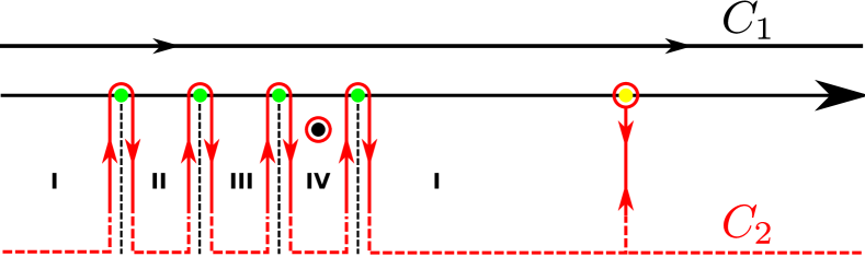
Figure 5: (color online) Deformation of the integration contour in the complex plane to study the intermediate and long time behavior. Green dots: van Hove singularities of the scattering states. Yellow dot: separated polaron pole. Black dot: complex pole of decaying state.

The green dots mark the positions of the van Hove singularities. The deformed contour $C_{2}$ (red) cannot overcome these points analytically. The contributions to the integral (V.2) from the path left and right of the singularities will not cancel each other because they lie on different sheets of the Riemann surface. We exemplify the (approximate) analysis of the integral by giving a concrete expression for the path around the lower band edge at $x_{\mathrm{s}}^{\mathrm{I/II}}=-\left(\frac{JS}{2}+\frac{W}{2}\right)$.

$$\alpha_{\mathbf{k}}^{\mathrm{I/II}}(t)=\frac{-1}{2\pi}\int\limits_{-\infty}^{0}\mathrm{d}x\>\mathrm{e}^{-i\left(x_{\mathrm{s}}^{\mathrm{I/II}}+ix\right)t}$$

$$\times\left(G_{\mathbf{k}\downarrow}^{\mathrm{I}}\left(x_{\mathrm{s}}^{\mathrm{I/II}}+ix\right)-G_{\mathbf{k}\downarrow}^{\mathrm{II}}\left(x_{\mathrm{s}}^{\mathrm{I/II}}+ix\right)\right)$$

$$= \frac{-1}{2\pi}\int\limits_{-\infty}^{0}\mathrm{d}x\>\mathrm{e}^{-i\left(x_{\mathrm{s}}^{\mathrm{I/II}}+ix\right)t}\left(C_{s}^{\mathrm{I/II}}\sqrt{x}+\mathcal{O}\left(x^{\frac{3}{2}}\right)\right)$$

$$= \frac{-i}{2\sqrt{\pi}}\mathrm{e}^{-ix_{\mathrm{s}}^{\mathrm{I/II}}t}\left(\frac{1}{2}C_{s}^{\mathrm{I/II}}t^{-\frac{3}{2}}+\mathcal{O}(t^{-\frac{5}{2}})\right).$$ (47)

The other van Hove singularities give rise to similar terms and we have summarized the explicit expressions for the coefficients $C_{s}$ in the appendix (D). From (47) we see, that the van Hove singularities contribute an oscillatory term with a frequency equal to the energetic position to $\alpha_{\mathbf{k}}(t)$. This term is damped in time with a decay rate given by a power law. The exponent of this power law depends only on the nature of the van Hove singularity, that is a square root singularity in our caseHöhler (1958).
For large enough $J$ there is a separated pole of the down-electron GF on the real axis shown as yellow dot in Fig. 5. If we denote the position of this pole by $x_{\mathrm{pol}}$ the contribution to $\alpha_{\mathbf{k}}(t)$ is given as the residue of the integrand in (V.2) at this point:

$$\alpha_{\mathbf{k}}^{\mathrm{pol}}(t) = \left.\frac{\mathrm{e}^{-ixt}}{1-JS\partial_{x}\left(\frac{1}{1-\frac{J}{2}G^{(0)}\left(x+\frac{JS}{2}\right)}\right)}\right|_{x=x_{\mathrm{pol}}}$$ (48)

$$= C_{\mathrm{pol}}\mathrm{e}^{-ix_{\mathrm{pol}}t}.$$

The characteristic oscillations of $P(t)$ visible in the upper panel of Fig. 4 are superpositions of the oscillatory terms in (47) and (48). They are damped in time as ($\sim t^{-\frac{3}{2}}$) at least. For large times only the contribution from (48) will survive and we get:

$$\lim_{t\to\infty}|\alpha_{\mathbf{k}}(t)|^{2}=|C_{\mathrm{pol}}|^{2}.$$ (49)

For large coupling strength $|J|\gg 1$ the pole position becomes approximately $x_{\mathrm{pol}}\approx\frac{J}{2}(S+1)$. Using the high energy expansion of the free GF in (48) we can derive an explicit result for $P(t)$ in this limit:

$$\lim_{t\to\infty}|\alpha_{\mathbf{k}}(t)|^{2}\stackrel{{\scriptstyle|J|\gg 1}}{{\approx}}\left(\frac{2S}{2S+1}\right)^{2}.$$ (50)

The electron polarization can be calculated from $P(t)$:

$$\left\langle\sigma_{z}\right\rangle(t)=\frac{\sum_{\mathbf{q}}|\beta_{\mathbf{k,q}}(t)|^{2}-|\alpha_{\mathbf{k}}(t)|^{2}}{2}=\frac{1}{2}-|\alpha_{\mathbf{k}}(t)|^{2},$$ (51)

where in the last step the normalization condition $\sum_{\mathbf{q}}|\beta_{\mathbf{k,q}}(t)|^{2}+|\alpha_{\mathbf{k}}(t)|^{2}=1$ is used.
We come now to the case of small $|J|$, when parts of the polaron band lie inside the scattering states. For those $\mathbf{k}$-values the initial down-electron will decay over time and vanish completely in the long time limit. One therefore expects an exponential decaying contribution to $\alpha_{\mathbf{k}}(t)$. As soon as the polaron peak runs into the scattering states there appear poles in regions II,III or IV of the analytic continuation of the down-electron GF that account for such an exponential term. This is depicted in Fig. 5 by the black dot in region IV. These poles contribute a term to $\alpha_{\mathbf{k}}(t)$ that equals (48) but now with a complex pole energy $x_{\mathrm{pol}}=x_{r}-i\gamma$.
There is one pole in each sheet of the different analytic continuations. In Fig. 6 (lower panel) the pole lines in the complex plane (parametrized by $\epsilon_{\mathbf{k}}$) are shown for $J=0.1$ eV. Whenever a pole has a real part $x_{r}$, that lies inside the energy region where the analytic continuation of the corresponding sheet has been performed (II, III or IV) it will add a term (48) to $\alpha_{\mathbf{k}}(t)$. The upper panel of Fig. 6 shows the free dispersion $\epsilon_{\mathbf{k}}$ for a path along the high symmetry lines in the first Brillouin zone.

Figure 6: (color online) Lower figure: Pole lines (parametrized by $\epsilon_{\mathbf{k}}$) in the different Riemann sheets. The colors of the lines denote the sheet where the poles can be found: red: II, green: III, blue: IV. When a pole lies in its window of visibility (dashed area with the same color) it gives an exponentially declining contribution to $\alpha_{\mathbf{k}}(t)$. The yellow line shows the positions of the polaron peak, when it lies outside the scattering region. Upper figure: Free electron dispersion $\epsilon_{\mathbf{k}}$ and the windows of visibility for the different poles. Parameters: $S=3.5$, $J=0.1$ eV and $W=1.0$ eV.

The $\epsilon_{\mathbf{k}}$ for which the corresponding pole is inside its region of visibility can be read off from the horizontal colored lines. Whenever this is the case, a pronounced (quasi particle) peak is visible in the down-electron spectral density, that lies approximately at the position of the real part of the pole $x_{r}$. We demonstrate this in Fig. 7 for two different values of $\epsilon_{\mathbf{k}}$.

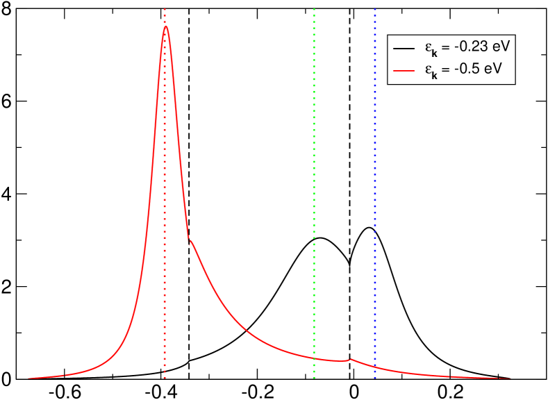
Figure 7: (color online) Down-electron spectral density for two different values of $\epsilon_{\mathbf{k}}$. Vertical black, dashed lines: position of the van Hove singularities. Vertical dotted lines: real part of the pole positions. Parameters: $S=3.5$, $J=0.1$ eV and $W=1.0$ eV.

For $\epsilon_{\mathbf{k}}=-0.5$ eV there is only a pole in region II (endpoint of the red pole-line). One finds a distinctive quasi-particle peak in the spectral density (red line) at approximately the real part of the pole position (vertical dotted line). An interesting constellation arises for $\epsilon_{\mathbf{k}}=-0.23$ eV. From Fig. 6 one can read off that two poles are now in their respective region (III,IV). Consequently two quasi-particle peaks can be found in the SD (black line). The negative imaginary part of the pole position can be interpreted as (half of) the inverse lifetime: $\tau\sim\frac{2}{\gamma}$. This is reflected directly by the width of the quasi-particle peaks, the smaller $\tau$ the broader the corresponding peak in the SD.
We had seen, that there are deviations from an exponential decay law at small times. The same is true for the long time limit. When $t\gg\frac{2}{\gamma}$ the exponentially decaying term (48) is damped away and only the contribution from the van Hove singularities (47) remain, which leads to a power law decay rate ($|\alpha_{\mathbf{k}}(t)|^{2}\sim t^{-3}$). It was first shown by KhalfinKhalfin (1958), that this deviation from exponential decay at large times is a general property of a system with a spectrum, that is bounded from below.
At the end of this section we want to discuss the long time behavior of a system, where we have chosen the initial conditions (41). If we deform the integration contour $C_{2}$ in (42) as shown in Fig. 5 and chose $J$ sufficiently small, so that $h_{1}(z)$ has no real root outside the scattering spectrum we get for large times:

$$\lim_{t\to\infty}\alpha_{\mathbf{k}}(t)=\mathrm{e}^{-i(\epsilon_{\mathbf{k-q_{n}}}-\frac{JS}{2})t}\times$$

$$\frac{1}{\sqrt{2NS}}\frac{-JS}{\epsilon_{\mathbf{k-q}}-\epsilon_{\mathbf{k}}-\frac{J}{2}(2S+1)-\frac{J}{2}\Phi_{\mathbf{k}}(\epsilon_{\mathbf{k-q}}+i0^{+})}.$$

This is indeed identical to the $\alpha_{\mathbf{q}}^{\mathbf{k}}$ coefficient found earlier for the scattering states (30) up to a trivial time dependent factor. For larger $J$ there will be additional terms coming from the real root of $h_{1}(z)$ which are not contained in the result of scattering theory. The reason for this are the persistent self-energy effects (cloud effects) already mentioned by van HoveHove (1955).

VII Summary and Conclusions

In this work we have revised the theory of the magnetic polaron to get a deeper understanding of one of the few exactly solvable limiting cases of the KLM.

First we have derived the complete eigenvalue spectrum of the finite lattice and the corresponding eigenstates are constructed.

In the limit of an infinite lattice parts of these eigenstates lose their norm and the eigenvalues of these states degenerate with the eigenvalues of the pure up-states. We then calculate the scattering states and show, that these states become the new eigenstates in this limit.

By solving the time-dependent Schrödinger equation for arbitrary initial conditions we are able to give a detailed analysis of the decay dynamics of the system. This is done for a down-electron with wavevector $\mathbf{k}$ prepared at $t=0$. For large exchange coupling $J$ the probability $P(t)$ to find a down-electron at time $t>0$ shows characteristic oscillations which are damped as $\sim t^{-\frac{3}{2}}$. We find the reason of these oscillations to be interference of different oscillatory terms with frequencies equal to the energetic positions of the van Hove singularities and the separated pole (polaron peak). For large times $P(t)$ becomes static with a value $P(t)<1$ and for $|J|\gg 1$ an explicit value can be derived.

For small coupling $J$ and $\epsilon_{\mathbf{k}}$ below a certain threshold $P(t)$ goes to zero over time - the down-electron decays. The main contribution to the decay dynamics stems from poles in the analytic continuation of the propagator giving rise to an exponential decay law. The imaginary part of the poles determines the lifetime of the down-electron.

We find deviations from an exponential decay law for small and large times. At $t=0$ the slope of $P(t)$ is zero. This leads to the quantum Zeno effect. At large times the exponential term is damped away and the decay behavior is solely determined by the contributions from the van Hove singularities. We get a power law decay ($P(t)\sim t^{-3}$) in this regime and there are also oscillations caused by interference effects.

The connection between certain initial conditions for the solution of the time-dependent Schrödinger equation and the retarded Green’s function approach as well as scattering theory is worked out. When a pure down-electron state is prepared at $t=0$ the time development of the down state coefficient of the wave function is given by the time-dependent down-electron spectral density, that can be obtained from the retarded Green’s function. Preparing an up-electron and a magnon at $t=0$ and taking the $t\to\infty$ limit the result of scattering theory (for the down-electron coefficient) can be reproduced for small $J$. For large $J$ however a new quasi-particle with infinite lifetime is created. Scattering theory is not able to describe this formation of a new quasi-particle.

The limiting case of the magnetic polaron is believed to describe the essential physics of the magnetic semiconductors EuO and EuS. For a realistic description of the quasi particle density of states of these materials one has to replace the model band structure (2) used in this work by a material specific one, that can be obtained from a ab initio band structure calculation. Such a calculation was done by Nolting et. al.Nolting et al. (1987) for EuO and Borstel et. al.Borstel et al. (1987) for EuS. From the experimental side the natural way of measuring the unoccupied states would be an inverse photoemission experiment. An alternative method is the two-photon photoemission spectroscopySteinmann (1989). This experimental technique can be used to get time and spin resolved spectral information with time resolutions down to the femtosecond and even attosecond regime Scholl et al. (1997); Pickel et al. (2006); Cavalieri et al. (2007). These new experimental methods could open up a possible road to a direct measurement of the decay dynamics of an (down) electron in the above mentioned prototypical compounds.

Appendix A Definitions scattering section

$$A_{1} = \frac{JS}{\epsilon_{\mathbf{k-q}}-\epsilon_{\mathbf{k}}-JS\pm i0^{+}},$$

$$A_{2} = \frac{J}{2N}\sum_{\mathbf{q^{\prime}}}\frac{1}{\epsilon_{\mathbf{k-q}}-\epsilon_{\mathbf{k-q^{\prime}}}\pm i0^{+}},$$

$$|Z_{1}\rangle = -\frac{J}{2}\sqrt{\frac{2S}{N}}\frac{|\mathbf{k}\downarrow;0\rangle}{\epsilon_{\mathbf{k-q}}-\epsilon_{\mathbf{k}}-JS\pm i0^{+}},$$

$$|Z_{2}\rangle = \frac{J}{2N}\sum_{\mathbf{q^{\prime}}}\frac{|\mathbf{k-q^{\prime}}\uparrow;\mathbf{q^{\prime}}\rangle}{\epsilon_{\mathbf{k-q}}-\epsilon_{\mathbf{k-q^{\prime}}}\pm i0^{+}}.$$ (53)

$$\hat{\mathbf{D}} =\frac{A_{2}}{2}\begin{pmatrix}1-\sqrt{4\frac{A_{1}}{A_{2}}+1}&0\\ 0&1+\sqrt{4\frac{A_{1}}{A_{2}}+1}\end{pmatrix},$$ (54)

$$\hat{\mathbf{U}} =\begin{pmatrix}-\frac{1}{2}-\sqrt{\frac{A_{1}}{A_{2}}+\frac{1}{4}}&-\frac{1}{2}+\sqrt{\frac{A_{1}}{A_{2}}+\frac{1}{4}}\\ 1&1\end{pmatrix}.$$ (55)

$$\alpha_{\mathbf{q}}^{\mathbf{k}} =\frac{1}{\sqrt{2NS}}\frac{-JS}{\epsilon_{\mathbf{k-q}}-\epsilon_{\mathbf{k}}-\frac{J}{2}(2S+1)-\frac{J}{2}\Phi_{\mathbf{k}}(\epsilon_{\mathbf{k-q}}\pm i0^{+})},$$

$$\beta_{\mathbf{q},\mathbf{q^{\prime}}}^{\mathbf{k}} =\delta_{\mathbf{q,q^{\prime}}}-\frac{1}{\sqrt{2NS}}\left(1+\frac{\epsilon_{\mathbf{k-q^{\prime}}}-\epsilon_{\mathbf{k}}}{\epsilon_{\mathbf{k-q}}-\epsilon_{\mathbf{k-q^{\prime}}}\pm i0^{+}}\right)\alpha_{\mathbf{q}}^{\mathbf{k}}.$$ (56)

$$\mathcal{R}_{\mathbf{q,q^{\prime}}}^{\mathbf{k}} = \frac{\alpha_{\mathbf{q}}^{\mathbf{k}}}{\sqrt{2NS}}\left\{\frac{2(\epsilon_{\mathbf{k-q}}-\epsilon_{\mathbf{k-q^{\prime}}})(\epsilon_{\mathbf{k-q}}-\epsilon_{\mathbf{k}})}{\epsilon_{\mathbf{k-q}}-\epsilon_{\mathbf{k-q^{\prime}}}\pm i0^{+}}\right.$$ (57)

$$\left.\pm i0^{+}\frac{2\epsilon_{\mathbf{k-q}}-\epsilon_{\mathbf{k-q^{\prime}}}-\epsilon_{\mathbf{k}}}{\epsilon_{\mathbf{k-q}}-\epsilon_{\mathbf{k-q^{\prime}}}\pm i0^{+}}\right\}$$

Appendix B Analytic continuation of $G^{(0)}(z)$

The simple cubic lattice Green’s function can be expressed in terms of the Gauss hypergeometric functionJoyce and Delves (2004):

$$G^{(0)}(z)=\mu_{1}(z)\left({}_{2}F_{1}\left(\frac{1}{3},\frac{2}{3};1;\eta_{1}(z)\right)\right)^{2}$$ (58)

with

$$\mu_{1}(z) = \frac{1}{2z}\left(3\sqrt{1-\frac{1}{z^{2}}}-\sqrt{1-\frac{9}{z^{2}}}\right),$$ (59)

$$\eta_{1}(z) = \frac{1}{8z^{2}}\left(4z^{2}+(9-4z^{2})\sqrt{1-\frac{9}{z^{2}}}-27\sqrt{1-\frac{1}{z^{2}}}\right).$$

This function is analytic in the complete complex plane with the exception of a branch cut on the real axis in the region $E_{B}\in-3\dots 3$ (bandwidth: $W=6$). When the real axis is crossed in this region, the imaginary part of (58) shows a discontinuity of $\Delta(x)=\pm 2\pi\rho(x)$ where $\rho(x)$ denotes the free density of states at point $x$.

Figure 8: (color online) Free GF slightly above the real axis. Vertical dashed lines: position of the van Hove singularities that form the boundaries for a possible analytic continuation below the real axis. Parameters: $W=1.0$ eV.

In Fig. 8 $G^{(0)}(x+i0^{+})$ is plotted slightly above the real axis. The clearly visible van Hove singularities at the band edges ($-3,3$) and at ($-1,1$) are limiting points for a possible analytic continuation over the branch cut. Therefore one reaches different Riemann sheets, depending on the section (II, III or IV) where the analytic continuation is performed.
To find these continuations we discuss firstly the analytic properties of the constituting functions. The square root function has branch points (of first order) at $0,-\infty$ and a branch cut connecting them on the negative real axis. Whenever one crosses this cut, one has to change the sign of the square root function to get an analytic continuation.
The hypergeometric function:

$$\mathrm{Hyp1}(z)={}_{2}F_{1}\left(\frac{1}{3},\frac{2}{3};1;x\right)$$ (60)

has a branch point of second order at the points $1,\infty$ and a branch cut on the real axis connecting them. Using formulas given in [Abramowitz and Stegun, 1964] one finds for the continuation from above to below the real axis:

$$\mathrm{Hyp2}(z) = (-z)^{-\frac{1}{3}}\frac{\Gamma\left(\frac{1}{3}\right)\mathrm{e}^{-i\frac{4\pi}{3}}}{\left(\Gamma\left(\frac{2}{3}\right)\right)^{2}}\>{}_{2}F_{1}\left(\frac{1}{3},\frac{1}{3};\frac{2}{3};\frac{1}{z}\right)$$

$$+ (-z)^{-\frac{2}{3}}\frac{\Gamma\left(-\frac{1}{3}\right)\mathrm{e}^{-i\frac{8\pi}{3}}}{\left(\Gamma\left(\frac{1}{3}\right)\right)^{2}}\>{}_{2}F_{1}\left(\frac{2}{3},\frac{2}{3};\frac{4}{3};\frac{1}{z}\right),$$

and from below to above the real axis:

$$\mathrm{Hyp3}(z) = (-z)^{-\frac{1}{3}}\frac{\Gamma\left(\frac{1}{3}\right)\mathrm{e}^{-i\frac{2\pi}{3}}}{\left(\Gamma\left(\frac{2}{3}\right)\right)^{2}}\>{}_{2}F_{1}\left(\frac{1}{3},\frac{1}{3};\frac{2}{3};\frac{1}{z}\right)$$

$$+ (-z)^{-\frac{2}{3}}\frac{\Gamma\left(-\frac{1}{3}\right)\mathrm{e}^{-i\frac{4\pi}{3}}}{\left(\Gamma\left(\frac{1}{3}\right)\right)^{2}}\>{}_{2}F_{1}\left(\frac{2}{3},\frac{2}{3};\frac{4}{3};\frac{1}{z}\right).$$

With this analysis it is now easy to find the analytic continuation of (58) from above to below the branch cut. To exemplify this, we discuss the continuation in region II. By crossing the real axis one also crosses the branch cut of the square root function $\sqrt{1+\frac{3}{x}}$. Defining new functions:

$$\mu_{2}(z) = \frac{1}{2z}\left(3\sqrt{1-\frac{1}{z^{2}}}+\sqrt{1-\frac{9}{z^{2}}}\right),$$ (63)

$$\eta_{2}(z) = \frac{1}{8z^{2}}\left(4z^{2}-(9-4z^{2})\sqrt{1-\frac{9}{z^{2}}}-27\sqrt{1-\frac{1}{z^{2}}}\right),$$

one then finds:

$$G_{\mathrm{II}}^{(0)}(z)=\mu_{2}(z)\left(\mathrm{Hyp1}(\eta_{2}(z))\right)^{2}$$ (64)

for the analytic continuation.

Figure 9: Analytic continuations of the free GF from above to below the real axis over the different branch cuts. Parameters: $W=1.0$ eV.

Similar results can be obtained for the other regions. They are summarized in Fig. 9. The two missing definitions are:

$$\mu_{3}(z) = -\frac{1}{2z}\left(3\sqrt{1-\frac{1}{z^{2}}}-\sqrt{1-\frac{9}{z^{2}}}\right),$$ (65)

$$\eta_{3}(z) = \frac{1}{8z^{2}}\left(4z^{2}-(9-4z^{2})\sqrt{1-\frac{9}{z^{2}}}+27\sqrt{1-\frac{1}{z^{2}}}\right).$$

Appendix C spectral moments

The moments of the down-electron spectral density are defined by:

$$M_{\mathbf{k}\downarrow}^{(n)}=\int\limits_{-\infty}^{\infty}\mathrm{d}EE^{n}S_{\mathbf{k}\downarrow}(E).$$ (66)

They can be calculated algebraically by the following ruleNolting (2009):

$$M_{\mathbf{k}\downarrow}^{(n)}=\left\langle[\underbrace{[\dots[[c_{\mathbf{k}\downarrow},H]_{-},H]_{-}\dots,H]_{-}}_{n-\mathrm{times}},c_{\mathbf{k}\downarrow}^{+}]_{+}\right\rangle.$$ (67)

We give the first four moments for the limiting case of the magnetic polaron:

$$M_{\mathbf{k}\downarrow}^{(0)} = 1,$$ (68)

$$M_{\mathbf{k}\downarrow}^{(1)} = \epsilon_{\mathbf{k}}+\frac{JS}{2},$$ (69)

$$M_{\mathbf{k}\downarrow}^{(2)} = \left(\epsilon_{\mathbf{k}}+\frac{JS}{2}\right)^{2}+\frac{J^{2}S}{2},$$ (70)

$$M_{\mathbf{k}\downarrow}^{(3)} = \left(\epsilon_{\mathbf{k}}+\frac{JS}{2}\right)^{3}$$ (71)

$$+J^{2}S(\epsilon_{\mathbf{k}}+J(S+1)/4).$$

Appendix D coefficients long time expansion

$$x_{s}^{\mathrm{I/II}} = -\left(\frac{JS}{2}+\frac{1}{2}\right):$$

$$C_{s}^{\mathrm{I/II}} = -\frac{4(-1)^{3/4}\text{Hyp1}\left(\frac{1}{4}\left(2-\sqrt{2}\right)\right)J^{2}S\left(3\sqrt{2}\text{Hyp1}^{\prime}\left(\frac{1}{4}\left(2-\sqrt{2}\right)\right)+2\text{Hyp1}\left(\frac{1}{4}\left(2-\sqrt{2}\right)\right)\right)}{\left((2\epsilon_{\mathbf{k}}+1)\left(\sqrt{2}\text{Hyp1}\left(\frac{1}{4}\left(2-\sqrt{2}\right)\right)^{2}J+1\right)+2JS\right)^{2}}$$ (72)

$$x_{s}^{\mathrm{II/III}} = -\left(\frac{JS}{2}+\frac{1}{6}\right):$$

$$C_{s}^{\mathrm{II/III}} = -\frac{(324-324i)\sqrt{3}\text{Hyp1}\left(\frac{1}{4}\left(2+5i\sqrt{2}\right)\right)J^{2}S\left(9i\text{Hyp1}^{\prime}\left(\frac{1}{4}\left(2+5i\sqrt{2}\right)\right)+\sqrt{2}\text{Hyp1}\left(\frac{1}{4}\left(2+5i\sqrt{2}\right)\right)\right)}{\left(6JS+(6\epsilon_{\mathbf{k}}+1)\left(1-3i\sqrt{2}\text{Hyp1}\left(\frac{1}{4}\left(2+5i\sqrt{2}\right)\right)^{2}J\right)\right)^{2}}$$ (73)

$$x_{s}^{\mathrm{III/IV}} = -\left(\frac{JS}{2}-\frac{1}{6}\right):$$

$$C_{s}^{\mathrm{III/IV}} = \frac{(324+324i)\sqrt{3}\text{Hyp1}\left(\frac{1}{4}\left(2-5i\sqrt{2}\right)\right)J^{2}S\left(\sqrt{2}\text{Hyp1}\left(\frac{1}{4}\left(2-5i\sqrt{2}\right)\right)-9i\text{Hyp1}^{\prime}\left(\frac{1}{4}\left(2-5i\sqrt{2}\right)\right)\right)}{\left(6JS+(6\epsilon_{\mathbf{k}}-1)\left(1-3i\sqrt{2}\text{Hyp1}\left(\frac{1}{4}\left(2-5i\sqrt{2}\right)\right)^{2}J\right)\right)^{2}}$$ (74)

$$x_{s}^{\mathrm{IV/I}} = -\left(\frac{JS}{2}-\frac{1}{2}\right):$$

$$C_{s}^{\mathrm{IV/I}} = \frac{4\sqrt[4]{-1}\text{Hyp1}\left(\frac{1}{4}\left(2-\sqrt{2}\right)\right)J^{2}S\left(3\sqrt{2}\text{Hyp1}^{\prime}\left(\frac{1}{4}\left(2-\sqrt{2}\right)\right)+2\text{Hyp1}\left(\frac{1}{4}\left(2-\sqrt{2}\right)\right)\right)}{\left((2\epsilon_{\mathbf{k}}-1)\left(\sqrt{2}\text{Hyp1}\left(\frac{1}{4}\left(2-\sqrt{2}\right)\right)^{2}J-1\right)-2JS\right)^{2}}$$ (75)

References

- Methfessel and Mattis (1968) S. Methfessel and D. C. Mattis, in Handb. Phys., edited by S. Flügge (Springer, 1968), vol. XVIII/1, p. 389.
- Nolting (1979a) W. Nolting, physica status solidi (b) 96, 11 (1979a), ISSN 1521-3951, URL http://dx.doi.org/10.1002/pssb.2220960102.
- Wachter (1979) P. Wachter, in Alloys and Intermetallics, edited by J. Karl A. Gschneidner and L. Eyring (Elsevier, 1979), vol. 2 of Handbook on the Physics and Chemistry of Rare Earths, pp. 507 – 574, URL http://www.sciencedirect.com/science/article/pii/S01681273790%20109.
- Salamon and Jaime (2001) M. B. Salamon and M. Jaime, Rev. Mod. Phys. 73, 583 (2001), URL http://link.aps.org/doi/10.1103/RevModPhys.73.583.
- Stier and Nolting (2007) M. Stier and W. Nolting, Phys. Rev. B 75, 144409 (2007), URL http://link.aps.org/doi/10.1103/PhysRevB.75.144409.
- Stier and Nolting (2008) M. Stier and W. Nolting, Phys. Rev. B 78, 144425 (2008), URL http://link.aps.org/doi/10.1103/PhysRevB.78.144425.
- Held and Vollhardt (2000) K. Held and D. Vollhardt, Phys. Rev. Lett. 84, 5168 (2000), URL http://link.aps.org/doi/10.1103/PhysRevLett.84.5168.
- Jungwirth et al. (2006) T. Jungwirth, J. Sinova, J. Mašek, J. Kučera, and A. H. MacDonald, Rev. Mod. Phys. 78, 809 (2006), URL http://link.aps.org/doi/10.1103/RevModPhys.78.809.
- Stier et al. (2011) M. Stier, S. Henning, and W. Nolting, Journal of Physics: Condensed Matter 23, 276006 (2011), URL http://stacks.iop.org/0953-8984/23/i=27/a=276006.
- Izumov and Medvedev (1971) Y. A. Izumov and M. V. Medvedev, Sov. Phys. JETP 32, 302 (1971).
- Richmond (1970) P. Richmond, Journal of Physics C: Solid State Physics 3, 2402 (1970), URL http://stacks.iop.org/0022-3719/3/i=12/a=004.
- Shastry and Mattis (1981) B. S. Shastry and D. C. Mattis, Phys. Rev. B 24, 5340 (1981), URL http://link.aps.org/doi/10.1103/PhysRevB.24.5340.
- Berciu and Sawatzky (2009) M. Berciu and G. A. Sawatzky, Phys. Rev. B 79, 195116 (2009), URL http://link.aps.org/doi/10.1103/PhysRevB.79.195116.
- Nolting (2009) W. Nolting, Fundamentals of Many-body Physics (Springer Berlin Heidelberg, 2009).
- Nolting (1979b) W. Nolting, Journal of Physics C: Solid State Physics 12, 3033 (1979b), URL http://stacks.iop.org/0022-3719/12/i=15/a=012.
- Sigrist et al. (1991) M. Sigrist, H. Tsunetsugu, and K. Ueda, Phys. Rev. Lett. 67, 2211 (1991), URL http://link.aps.org/doi/10.1103/PhysRevLett.67.2211.
- Hove (1955) L. V. Hove, Physica 21, 901 (1955), ISSN 0031-8914, URL http://www.sciencedirect.com/science/article/pii/S00318914559%28329.
- Hove (1957) L. V. Hove, Physica 23, 441 (1957), ISSN 0031-8914, URL http://www.sciencedirect.com/science/article/pii/S00318914579%28914.
- Nakanishi (1958) N. Nakanishi, Progress of Theoretical Physics 19, 607 (1958), URL http://ptp.ipap.jp/link?PTP/19/607/.
- Höhler (1958) G. Höhler, Zeitschrift für Physik A Hadrons and Nuclei 152, 546 (1958), ISSN 0939-7922, 10.1007/BF01375212, URL http://dx.doi.org/10.1007/BF01375212.
- Khalfin (1958) S. A. Khalfin, Sov. Phys. JETP 6, 1053 (1958).
- Misra and Sudarshan (1977) B. Misra and E. C. G. Sudarshan, Journal of Mathematical Physics 18, 756 (1977), URL http://link.aip.org/link/?JMP/18/756/1.
- Chiu et al. (1977) C. B. Chiu, E. C. G. Sudarshan, and B. Misra, Phys. Rev. D 16, 520 (1977), URL http://link.aps.org/doi/10.1103/PhysRevD.16.520.
- Sudarshan et al. (1978) E. C. G. Sudarshan, C. B. Chiu, and V. Gorini, Phys. Rev. D 18, 2914 (1978), URL http://link.aps.org/doi/10.1103/PhysRevD.18.2914.
- Parravicini et al. (1980) G. Parravicini, V. Gorini, and E. C. G. Sudarshan, Journal of Mathematical Physics 21, 2208 (1980), URL http://link.aip.org/link/?JMP/21/2208/1.
- Sudarshan and Chiu (1993) E. C. G. Sudarshan and C. B. Chiu, Phys. Rev. D 47, 2602 (1993), URL http://link.aps.org/doi/10.1103/PhysRevD.47.2602.
- Lippmann and Schwinger (1950) B. A. Lippmann and J. Schwinger, Phys. Rev. 79, 469 (1950), URL http://link.aps.org/doi/10.1103/PhysRev.79.469.
- Nolting et al. (1987) W. Nolting, G. Borstel, and W. Borgiel, Phys. Rev. B 35, 7015 (1987), URL http://link.aps.org/doi/10.1103/PhysRevB.35.7015.
- Borstel et al. (1987) G. Borstel, W. Borgiel, and W. Nolting, Phys. Rev. B 36, 5301 (1987), URL http://link.aps.org/doi/10.1103/PhysRevB.36.5301.
- Steinmann (1989) W. Steinmann, Applied Physics A: Materials Science & Processing 49, 365 (1989), ISSN 0947-8396, 10.1007/BF00615019, URL http://dx.doi.org/10.1007/BF00615019.
- Scholl et al. (1997) A. Scholl, L. Baumgarten, R. Jacquemin, and W. Eberhardt, Phys. Rev. Lett. 79, 5146 (1997), URL http://link.aps.org/doi/10.1103/PhysRevLett.79.5146.
- Pickel et al. (2006) M. Pickel, A. Schmidt, M. Donath, and M. Weinelt, Surface Science 600, 4176 (2006), ISSN 0039-6028, URL http://www.sciencedirect.com/science/article/pii/S00396028060%05437.
- Cavalieri et al. (2007) A. L. Cavalieri, N. Muller, T. Uphues, V. S. Yakovlev, A. Baltuska, B. Horvath, B. Schmidt, L. Blumel, R. Holzwarth, S. Hendel, et al., Nature 449, 1029 (2007), ISSN 0028-0836, URL http://dx.doi.org/10.1038/nature06229.
- Joyce and Delves (2004) G. S. Joyce and R. T. Delves, Journal of Physics A: Mathematical and General 37, 3645 (2004), URL http://stacks.iop.org/0305-4470/37/i=11/a=008.
- Abramowitz and Stegun (1964) M. Abramowitz and I. Stegun, Handbook of Mathematical Functions: With Formulas, Graphs, and Mathematical Tables, Applied mathematics series (Dover Publications, 1964), ISBN 9780486612720.