Realized Laplace transforms for pure-jump semimartingales

Abstract

We consider specification and inference for the stochastic scale of discretely-observed pure-jump semimartingales with locally stable Lévy densities in the setting where both the time span of the data set increases, and the mesh of the observation grid decreases. The estimation is based on constructing a nonparametric estimate for the empirical Laplace transform of the stochastic scale over a given interval of time by aggregating high-frequency increments of the observed process on that time interval into a statistic we call realized Laplace transform. The realized Laplace transform depends on the activity of the driving pure-jump martingale, and we consider both cases when the latter is known or has to be inferred from the data.

T1Supported in part by NSF Grant SES-0957330.

and

1 Introduction

Continuous-time semimartingales are used extensively for modeling many processes in various areas, particularly in finance. Typically the model of interest is an Itô semimartingale (semimartingale with absolute continuous characteristics) given by

$$dX_{t}=\alpha_{t}\,dt+\sigma_{t-}\,dZ_{t}+dY_{t},$$ (1)

where $\alpha_{t}$ and $\sigma_{t}$ are some processes with càdlàg paths, $Z_{t}$ is an infinite variation Lévy martingale and $Y_{t}$ is a finite variation jump process satisfying certain regularity conditions (all technical conditions on the various processes will be given later). The martingale $Z_{t}$ can be continuous (i.e., Brownian motion), jump-diffusion or of pure-jump type (i.e., without a continuous component). The presence of the last term in (1) might appear redundant, as $Z_{t}$ can already contain jumps, but its presence will allow us to encompass also the class of time-changed Lévy processes in our analysis. In any case, this last term in (1) is dominated over small scales by the term involving $Z_{t}$.

Our interest in this paper will be in inference to the process $\sigma_{t}$ when $Z_{t}$ is a pure-jump Lévy process. Pure-jump models have been used to study various processes of interest such as volatility and volume of financial prices BNS01 , Davis , traffic data Mikosch and electricity prices Kluppelberg .

Parametric or nonparametric estimation of a model satisfying (1) in the pure-jump case is quite complicated for at least the following reasons. First, very often the transitional density of $X_{t}$ is not known in closed-form. This holds true, even in the relatively simple case when $X_{t}$ is a pure-jump Lévy process. Second, in many situations the realistic specification of $\sigma_{t}$ often implies that $X_{t}$ is not a Markov process, with respect to its own filtration, and hence all developed methods for estimation of the latter will not apply. Third, the various parameters of the model (1) capture different statistical properties of the process $X_{t}$ and hence will have various rates of convergence depending on the sampling scheme. For example, in general, $\alpha_{t}$ and the tails of $Z_{t}$ can be estimated consistently only when the span of the data increases, whereas the so-called activity of $Z_{t}$ can be recovered even from a fixed-span data set, provided the mesh of the latter decreases; see B10 for estimation of the activity from low-frequency data set. Finally, the simulation of the process $X_{t}$ can be, in many cases, difficult or time consuming.

In view of the above-mentioned difficulties, our goal here is specification analysis for only part of the model, mainly the process $\sigma_{t}$, in the case when $X_{t}$ is a pure-jump process following (1). We conduct inference in the case when we have a high-frequency data set of $X_{t}$ with increasing time span; see B10 and NR for inference about jump processes based on low frequency. We refer to $\sigma_{t}$ as the stochastic scale of the pure-jump process $X_{t}$ in analogy with the scale parameter of a stable process, that is, when $X_{t}$ is a stable process then the constant $\sigma$ is the scale of the process. $\sigma_{t}$ is key in the specification of (1) and, in particular, it captures the time-variation of the process $X_{t}$ over small intervals of time. Our goal here will be to make the inference about $\sigma_{t}$ robust to the rest of the components of the model, that is, the specification of $\alpha_{t}$ and $Y_{t}$, as well as the dependence between $\sigma_{t}$ and $Z_{t}$.

The inference in the paper is for processes for which the Lévy measure of the driving martingale $Z_{t}$ in (1) behaves around zero like that of a stable process. This covers, of course, the stable process, but also many other Lévy processes of interest with details provided in Section 2 below. The idea of our proposed method of inference is to use the fact that when $Z_{t}$ is locally stable, the leading component of the process $X_{t}$ over small scales is governed by that of the “stable component” of $Z_{t}$. Moreover, when $\sigma_{t}$ is an Itô semimartingale, then “locally” its changes are negligible and $\sigma_{t}$ can be treated as constant. Intuitively then infill asymptotics can be conducted as if the increments of $X_{t}$ are products of (a locally constant) stochastic scale and independent i.i.d. stable random variables. This, in particular, implies that the empirical characteristic function of the high-frequency increments over a small interval of time will estimate the characteristic function of a scaled stable process. The latter, however, is the Laplace transform for the locally constant stochastic scale. Therefore, aggregating over a fixed interval time the empirical characteristic function of the (appropriately re-scaled) high-frequency increments of $X_{t}$ provides a nonparametric estimate for the empirical Laplace transform of the stochastic scale over that interval. We refer to this simple statistic as realized Laplace transform for pure-jump processes. The connection between the empirical characteristic function of the driving martingale and the Laplace transform of the stochastic scale in the context of time-changed Lévy processes, with time-change independent of the driving martingale, has been previously used for low-frequency estimation in B11 .

The inference based on the realized Laplace transform is robust to the specification of $\alpha_{t}$, as well as the tail behavior of $Z_{t}$. Intuitively, this is due to our use of the high-frequency data whose marginal law is essentially determined by the small jumps of $Z_{t}$ and the stochastic scale $\sigma_{t}$. Quite naturally, however, our inference depends on the activity of the small jumps of the driving martingale $Z_{t}$. The latter corresponds to the index of the stable part of $Z$, and using the self-similarity of the stable process, it determines its scaling over different (high) frequencies. Therefore, the activity index enters directly into the calculation of the realized Laplace transform. We conduct inference, both in the case where the activity is assumed known, and when it needs to be estimated from the data. The estimation of the activity index, however, differs from the inference for the stochastic scale. While for the latter we need, in general, the time-span to increase to infinity (except for the degenerate case when $\sigma_{t}$ is actually constant), for the former, this is not the case. The activity index can be estimated only with a fixed span of high-frequency data, and, in general, increasing time-span will not help for its nonparametric estimation. Therefore, we estimate the activity index of $Z_{t}$ using the initial part of the sample with a fixed span and then plug it into the construction of the realized Laplace transform. We further quantify the asymptotic effect from this plug-in approach on the inference for the Laplace transform of the stochastic scale.

The Laplace transform of the stochastic scale preserves the information for its marginal distribution. Therefore, it can be used for efficient estimation and specification testing. We illustrate this in a parametric setting by minimizing the distance between our nonparametric Laplace estimate and a model implied one, which is similar to estimation based on the empirical characteristic function, as in Feuerverger .

Finally, the current paper studies the realized Laplace transform for the case when $Z_{t}$ is pure-jump, while TT10 (and the empirical application of it in TTG11 ) consider the case where $Z_{t}$ is a Brownian motion. The pure-jump case is substantively different, starting from the very construction of the statistic as well as its asymptotic behavior. The leading component in the asymptotic expansions in the pure-jump case is a stable process with an index of less than $2$, and this index is, in general, unknown and needs to be estimated, which further necessitates different statistical analysis from the continuous case. Also, the residual components in $X_{t}$, like $\alpha_{t}$, play a more prominent role when $X_{t}$ is of pure-jump type, and when the activity is low this requires modifying appropriately the realized Laplace transform to purge them.

The paper is organized as follows. Section 2 presents the formal setup and assumptions. Section 3 introduces the realized Laplace transform and derives its limit behavior. In Section 4 we conduct a Monte Carlo study, and in Section 5 we present a parametric application of the developed limit theory. Section 6 concludes. The proofs are given in Section 7.

2 Setting and assumptions

Throughout the paper, the process of interest is denoted with $X_{t}$ and is defined on some filtered probability space $(\Omega,\mathcal{F},(\mathcal{F}_{t})_{t\geq 0},\mathbb{P})$. Before stating our assumptions, we recall that a Lévy process $L_{t}$ with characteristic triplet $(b,c,\nu)$ with respect to truncation function $\kappa(x)=x$ (we will always assume that the process has a finite first order moment) is a process with characteristic function given by

$$\mathbb{E}(e^{iuL_{t}})=\exp\biggl{(}t\biggl{(}iub-u^{2}c/2+\int_{\mathbb{R}}(e^{iux}-1-iux)\nu(dx)\biggr{)}\biggr{)}.$$ (2)

With this notation, we assume that the Lévy process $Z_{t}$ in (1) has a characteristic triplet $(0,0,\nu)$ for $\nu$ some Lévy measure. Note that since the truncation function with respect to which the characteristics of the Lévy processes are presented is the identity, the above implies that $Z_{t}$ is a pure-jump martingale. The first term in (1) is the drift term. It captures the persistence in the process, and when $X_{t}$ is used to model financial prices, the drift captures compensation for risk and time. The second term in (1) is defined in a stochastic sense, since in Assumption A below, we will assume that $Z_{t}$ is of infinite variation. The last term in (1) is a finite variation pure-jump process. Assumption A below will impose some restrictions on its properties, but we stress that there is no assumption of independence between the processes $\sigma_{t}$, $Z_{t}$ and $Y_{t}$.

In the pure-jump model the jump martingale, $Z_{t}$ substitutes the Brownian motion used in jump-diffusions to model the “small” moves. We note that the “dominant” part of the increment of $X_{t}$ over a short interval of time $(t,t+\Delta)$ is $\sigma_{t-}\times(Z_{t+\Delta}-Z_{t})$. This term is of order $O_{p}(\Delta^{\alpha})$ for $\alpha\in[1/2,1)$, while the rest of the components of $X_{t}$ are at most $O_{p}(\Delta)$ when $\Delta\downarrow 0$.

We recall from the introduction that our object of interest in this paper is the stochastic scale of the martingale component of $X_{t}$, that is, $\sigma_{t}$. Of course we observe only $X_{t}$ and $\sigma_{t}$ is hidden into it, so our goal in the paper will be to uncover $\sigma_{t}$, and its distribution in particular, with assuming as little as possible about the rest of the components of $X_{t}$ and the specification of $\sigma_{t}$ itself (including the activity of the driving martingale). Given the preceding discussion, the scaling of the driving martingale components over short intervals of time will be of crucial importance for us, as, at best, we can observe only a product of the stochastic scale with $Z_{t,t+\Delta}$. Our Assumption A below characterizes the behavior of $Z_{t}$ and $Y_{t}$ over small scales.

Assumption A

The Lévy density of $Z_{t}$, $\nu$, is given by

$$\nu(x)=\frac{A}{|x|^{\beta+1}}+\nu^{\prime}(x),\qquad\beta\in(1,2),\qquad\int_{\mathbb{R}}|x|\nu(x)\,dx<\infty,$$ (3)

where

$$A=\biggl{(}\frac{4\Gamma(2-\beta)|\cos(\beta\pi/2)|}{\beta(\beta-1)}\biggr{)}^{-1},\qquad\beta\in(1,2)$$ (4)

and further there exists $x_{0}>0$ such that for $|x|\leq x_{0}$ we have $|\nu^{\prime}(x)|\leq\frac{C}{|x|^{\beta^{\prime}+1}}$ for some $\beta^{\prime}<1$ and a constant $C\geq 0$.

We further have $Y_{t}$ absolutely integrable and $\mathbb{E}|Y_{t}-Y_{s}|^{\beta^{\prime}}<C|t-s||\log|t-s||$ for every $t,s\geq 0$ with $|t-s|\leq 1$, some positive constant $C$, and $\beta^{\prime}<1$ being the constant above.

Assumption A implies that the small scale behavior of the driving martingale $Z_{t}$ is like that of a stable process with index $\beta$. The index $\beta$ determines the “activity” of the driving process, that is, the vibrancy of its trajectories, and thus henceforth we will refer to it as the activity. Formally, $\beta$ equals the Blumenthal–Getoor index of the Lévy process $Z_{t}$. The value of the index $\beta$ is crucial for recovering $\sigma_{t}$ from the discrete data on $X_{t}$, as intuitively it determines how big on average the increments $Z_{t,t+\Delta}$ should be for a given sampling frequency. The following lemma makes this formal.

Lemma 1.

Let $Z_{t}$ satisfy Assumption A. Then for $h\rightarrow 0$, we have

$$h^{-1/\beta}Z_{th}\stackrel{{\scriptstyle\mathcal{L}}}{{\longrightarrow}}S_{t},$$ (5)

where the convergence is for the Skorokhod topology on the space of càdlàg functions. $\mathbb{R}_{+}\rightarrow\mathbb{R}$, and $S_{t}$ is a stable process with characteristic function $\mathbb{E}(e^{iuS_{1}})=e^{-|u|^{\beta}/2}$.

The value of the constant $A$ in (4) is a normalization that we impose. We are obviously free to do that since what we observe is $X_{t}$, whose leading component over small scales is an integral of $\sigma_{t}$, with respect to the jump martingale $Z_{t}$, and we never observe the two separately. The above choice of $A$ is a convenient one that ensures that when $\beta\rightarrow 2$, the jump process converges finite-dimensionally to Brownian motion. We note that in Assumption A we rule out the case $\beta\leq 1$, but this is done for brevity of exposition, as most processes of interest are of infinite variation (although we rule out some important processes like the generalized hyperbolic).

In Assumption A we restrict the “activity” of the “residual” jump components of $X_{t}$; that is, we limit their effect in determining the small moves of $X$. The effect of the “residual” jump components on the small moves is controlled by the parameter $\beta^{\prime}$. From (3), the leading component of $\nu(x)$ is the Lévy density of a stable, and $\nu^{\prime}(x)$ is the residual one. The restriction $\beta^{\prime}<1$, implies that the “residual” jump component is of finite variation. This restriction is not necessary for convergence in probability results (only $\beta^{\prime}<\beta$ is needed for this), but is probably unavoidable if one needs also the asymptotic distribution of the statistics that we introduce in the paper. In most parametric models this restriction is satisfied.

We note that $\nu^{\prime}(x)$ in (3) is a signed measure, and therefore Assumption A restricts only the behavior of $\nu(x)$ for $x\sim 0$ to be like that of a stable process. However, for the big jumps, that is, when $|x|>K$ for some arbitrary $K>0$, the stable part of $\nu(x)$ can be completely eliminated or tempered by negative values of the “residual” $\nu^{\prime}(x)$. An example of this, which is covered by our Assumption A, is the tempered stable process of Ro04 , generated from the stable by tempering its tails, which has all of its moments finite. Therefore, while Assumption A ties the small scale behavior of the driving martingale $Z_{t}$ with that of a stable process, it leaves its large scale behavior unrestricted (i.e., the limit of $h^{-\alpha}Z$th for some $\alpha>0$ when $h\rightarrow\infty$ is unrestricted by our assumption) and thus, in particular, unrelated with that of a stable process.

Remark 1.

Assumption A is analogous to the assumption used in SJ07 . It is also related to the so-called regular Lévy processes of exponential type, studied in BL02 , with $\beta=\nu$ in the notation of that paper. Compared with the above mentioned processes of BL02 , we impose slightly more structure on the Lévy density around zero but no restriction outside of it. We note that if Assumption A fails, then the results that follow are not true. The degree of the violation depends on the sampling frequency and the deviation of the characteristic function of $Z$ over small scales from that of a stable.

Finally, the process $Y_{t}$ also captures a “residual” jump component of $X_{t}$ in terms of its small scale behavior. Assumption A limits its activity by $\beta^{\prime}$. The component of $Z$ corresponding to $\nu^{\prime}(x)$ and $Y_{t}$ control the jump measure of $X_{t}$ away from zero. Unlike the former, whose time variation is determined by $\sigma_{t}$, the latter has essentially unrestricted time variation. There is clearly some “redundancy” in the specification in (1) in terms of modeling the jumps of $Z_{t}$ away from zero, but this is done to cover more general pure-jump models, as we make clear from the following two remarks.

Remark 2.

Assumption A nests time-changed Lévy processes with absolute continuous time changes (see, e.g., CGMY03 ), that is, specifications of the form

$$dX_{t}=\alpha_{t}\,dt+\int_{0}^{t}\int_{\mathbb{R}}x\widetilde{\mu}(ds,dx),$$ (6)

where $\mu$ is a random integer-valued measure with compensator $a_{t}\,dt\otimes\nu(dx)$ for some nonnegative process $a_{t}$ and Lévy measure $\nu(dx)$ satisfying (3) of Assumption A and $\widetilde{\mu}=\mu-\nu$. This can be shown using Theorem 14.68 of Jacod79 or Theorem 2.1.2 of JP , linking integrals of random functions with respect to Poisson measure and random integer-valued measures, and implies that $X_{t}$ in (6) can be equivalently represented as (1) with $\sigma_{t}$ given by $a_{t}^{1/\beta}$.

On the other hand, if we start with $X$ given by (1), with $Z$ strictly stable and no $Y$, we can show, using the definition of jump compensator and Theorem II.1.8 of JS , that the latter is a time-changed Lévy process with time change $|\sigma_{t-}|^{\beta}$. For more general “stable-like” Lévy processes, we need to introduce an additional term [this is $Y_{t}$ in (1)] in addition to the above time-changed stable process.

We note that the connection of (1) with the time-changed Lévy processes does not depend on the presence of any dependence between $\sigma_{t}$ and $Z_{t}$.

Remark 3.

Assumption A is also satisfied by the pure-jump Lévy-driven CARMA models (continuous-time autoregressive moving average) which have been used for modeling series exhibiting persistence; see, for example, BR01a and the many references therein. For these processes $\sigma_{t}$ in (1) is a constant.

Our next assumption imposes minimal integrability conditions on $\alpha_{t}$ and $\sigma_{t}$ and further limits the amount of variation in these processes over short periods of time. Intuitively, we will need the latter to guarantee that by sampling frequently enough we can treat “locally” $\sigma_{t}$ (and $\alpha_{t}$) as constant.

Assumption B

The process $\sigma_{t}$ is an Itô semimartingale given by

$$\sigma_{t}=\sigma_{0}+\int_{0}^{t}\tilde{\alpha}_{s}\,ds+\int_{0}^{t}\tilde{\sigma}_{s}\,dW_{s}+\int_{0}^{t}\int_{\mathbb{R}}\underline{\delta}(s-,x)\underline{\tilde{\mu}}(ds,dx),$$ (7)

where $W$ is a Brownian motion; $\underline{\mu}$ is a homogenous Poisson measure, with Lévy measure $\underline{\nu}(dx)$, having arbitrary dependence with $\mu$, for $\mu$ being the jump measure of $Z$. We assume $|\underline{\delta}(t,x)|\leq\gamma_{t}\underline{\delta}(x)$ for some integrable process $\gamma_{t}$ and $\int_{\mathbb{R}}(\underline{\delta}(x)\wedge 1)^{\beta^{\prime\prime}}\underline{\nu}(dx)<\infty$ for some $\beta^{\prime\prime}<2$. Further, for every $t$ and $s$, we have

$$\cases{\displaystyle\mathbb{E}\biggl{(}\alpha_{t}^{2}+\sigma_{t}^{2}+\tilde{\alpha}_{t}^{2}+\tilde{\sigma}_{t}^{2}+(\tilde{\sigma}_{t}^{\prime})^{2}+\int_{\mathbb{R}}\underline{\delta}^{2}(t,x)\underline{\nu}(dx)\biggr{)}<C,\cr\displaystyle\mathbb{E}\biggl{(}|\alpha_{t}-\alpha_{s}|^{2}+|\tilde{\sigma}_{t}-\tilde{\sigma}_{s}|^{2}+\int_{\mathbb{R}}\bigl{(}\underline{\delta}(t,x)-\underline{\delta}(s,x)\bigr{)}^{2}\underline{\nu}(dx)\biggr{)}<C|t-s|,}$$ (8)

where $C>0$ is some constant that does not depend on $t$ and $s$.

Assumption B imposes $\sigma_{t}$ to be an Itô semimartingale. This is a relatively mild assumption satisfied by the popular multifactor affine jump-diffusions DFS03 as well as the CARMA Lévy-driven models used to model persistent processes BR01a . Assumption B rules out certain long-memory specifications for $\sigma_{t}$, although we believe that, at least for some of them, the results in this paper will continue to hold.

Importantly, however, Assumption B allows for jumps in the stochastic scale that can have arbitrary dependence with the jumps in $X_{t}$ which is particularly relevant for modeling financial data, for example, in the parametric models of COGARCH . Finally, the second part of (8) will be satisfied when the corresponding processes are Itô semimartingales. The next Assumption B^′ restricts Assumption B in a way that will allow us to strengthen some of the theoretical results in the next section.

Assumption B^′

The process $\sigma_{t}$ is an Itô semimartingale given by

$$\sigma_{t}=\sigma_{0}+\int_{0}^{t}\!\tilde{\alpha}_{s}\,ds+\int_{0}^{t}\!\tilde{\sigma}_{s}\,dW_{s}+\int_{0}^{t}\!\tilde{\sigma}^{\prime}_{s}\,dZ_{s}+\int_{0}^{t}\int_{\mathbb{R}}\underline{\delta}(s-,x)\underline{\tilde{\mu}}(ds,dx),$$ (9)

with the same notation as Assumption B, with the only difference being that $\underline{\mu}$ is now independent from $\mu$. We also assume that corresponding condition (8) holds as well as that $Z_{t}$ is square-integrable.

The strengthening in Assumption B^′ is in the modeling of the dependence between the jumps in $X_{t}$ and $\sigma_{t}$. In Assumption B^′, this is done via the third integral in (9). This is similar to modeling dependence between continuous martingales using correlated Brownian motions. What is ruled out by Assumption B^′ is dependence between the jumps in $X_{t}$ and $\sigma_{t}$ that is different for the jumps of different size. Assumption B^′ will be satisfied when the pair $(X_{t},\sigma_{t})$ are modeled jointly via a Lévy-driven SDE.

Finally, in our estimation we make use of long-span asymptotics for the process $\sigma_{t}$ and the latter contains temporal dependence. Therefore, we need a condition on this dependence that guarantees that a central limit theorem for the associated empirical process exists. This condition is given next.

Assumption C

The volatility $\sigma_{t}$ is a stationary and $\alpha$-mixing process with $\alpha_{t}^{\mathrm{mix}}=O(t^{-3-\iota})$ for arbitrarily small $\iota>0$ when $t\rightarrow\infty$, where

$$\alpha_{t}^{\mathrm{mix}} = \sup_{A\in\mathscr{F}_{0},B\in\mathscr{F}^{t}}|\mathbb{P}(A\cap B)-\mathbb{P}(A)\mathbb{P}(B)|,$$

$$\mathscr{F}_{0} = \sigma(\sigma_{s},s\leq 0)\qquad\mbox{and}\qquad\mathscr{F}^{t}=\sigma(\sigma_{s},s\geq t).$$

3 Limit theory for RLT of pure-jump semimartingales

Now we are ready to formally define the realized Laplace transform for the pure-jump model and derive its asymptotic properties. We assume the process $X_{t}$ is observed at the equidistant times $0,\Delta_{n},\ldots,i\Delta_{n},\ldots,[T/\Delta_{n}]$ where $\Delta_{n}$ is the length of the high-frequency interval, and $T$ is the span of the data. The realized Laplace transform is then defined as

$$V_{T}(X,\Delta_{n},\beta,u)=\sum_{i=1}^{[T/\Delta_{n}]}\Delta_{n}\cos((2u)^{1/\beta}\Delta_{n}^{-1/\beta}\Delta_{i}^{n}X),$$

(10)

$$\eqntext{\Delta_{i}^{n}X=X_{i\Delta_{n}}-X_{(i-1)\Delta_{n}},}$$ (11)

where $\beta$ is the activity index of the driving martingale $Z_{t}$ given in its Lévy density in (3). $V_{T}(X,\Delta_{n},\beta,u)$ is the real part of the empirical characteristic function of the appropriately scaled increments of the process $X_{t}$. In the case of jump-diffusions, $\beta$ in (3) is replaced with $2$ as the activity of the Brownian motion has an index of $2$ (i.e., for the Brownian motion, Lemma 1 holds with $\beta$ replaced by $2$). We show in this section that $V_{T}(X,\Delta_{n},\beta,u)/T$ is a consistent estimator for the empirical Laplace transform of $|\sigma_{t}|^{\beta}$ and further derive its asymptotic properties under various sampling schemes as well as assumptions regarding whether $\beta$ is known or needs to be estimated.

3.1 Fixed-span asymptotics

We start with the case when $T$ is fixed and $\Delta_{n}\rightarrow 0$, that is, the infill asymptotics, and we further assume we know $\beta$. Since the driving martingale over small scales behaves like $\beta$-stable (Assumption A) and the stochastic scale changes over short intervals are not too big on average (Assumption B), then the “dominant” part (in a infill asymptotic sense) of the increment $\Delta_{i}^{n}X$ (when $\Delta_{n}$ is small) is $\sigma_{(i-1)\Delta_{n}}\Delta_{i}^{n}Z$. $\Delta_{i}^{n}Z$ is approximately stable, and from Lemma 1, we have approximately $\Delta_{i}^{n}Z\stackrel{{\scriptstyle d}}{{=}}\Delta_{n}^{1/\beta}\times Z_{1}$ with the characteristic function of $Z_{1}$ given by $e^{-|u|^{\beta}/2}$. Therefore, for a fixed $T$, $V_{T}(X,\Delta_{n},\beta,u)$ is approximately a sample average of a heteroscedastic data series. Thus, by the law of large numbers (when $\Delta_{n}\rightarrow 0$), it will converge to $\int_{0}^{T}e^{-u|\sigma_{t}|^{\beta}}\,ds$, which is the empirical Laplace transform of $|\sigma_{t}|^{\beta}$ after dividing by $T$. The following theorem gives the precise infill asymptotic result. In it we denote with $\mathcal{L}-s$ convergence stable in law, which means that the convergence in law holds jointly with any random variable defined on the original probability space.

Theorem 1.

For the process $X_{t}$, assume that Assumptions A and B hold with $\beta^{\prime}<\beta/2$, and let $\Delta_{n}\rightarrow 0$ with $T$ fixed.

If $\beta>4/3$, then we have

$$\frac{1}{\sqrt{\Delta_{n}}}\biggl{(}V_{T}(X,\Delta_{n},\beta,u)-\int_{0}^{T}e^{-u|\sigma_{s}|^{\beta}}\,ds\biggr{)}$$

(12)

$$\qquad\stackrel{{\scriptstyle\mathcal{L}-s}}{{\longrightarrow}}\sqrt{\int_{0}^{T}F_{\beta}(u^{1/\beta}|\sigma_{s}|)\,ds}\times E,$$

where $E$ is a standard normal variable defined on an extension of the original probability space and independent from the $\sigma$-field $\mathcal{F}$; $F_{\beta}(x)=\frac{e^{-2^{\beta-1}x^{\beta}}-2e^{-x^{\beta}}+1}{2}$ for $x>0$.

A consistent estimator for the asymptotic variance is given by

$$\frac{V_{T}(X,\Delta_{n},\beta,2^{\beta-1}u)-2V_{T}(X,\Delta_{n},\beta,u)+1}{2}.$$ (13)

If $\beta\leq 4/3$, then

$$\biggl{(}V_{T}(X,\Delta_{n},\beta,u)-\int_{0}^{T}e^{-u|\sigma_{s}|^{\beta}}\,ds\biggr{)}=O_{p}(\Delta_{n}^{2-2/\beta}).$$ (14)

In the case when $X_{t}$ is a Lévy process, or, more generally, when only the scale $\sigma_{t}$ is constant as is the case for the Lévy-driven CARMA models, the above theorem can be used to estimate the scale coefficient $\sigma$ by either fixing some $u$ or using a whole range of $u$’s as in the methods for estimation of stable processes based on the empirical characteristic function; see, for example, Koutrouvelis and SJ06 . Furthermore, this can be done jointly with the nonparametric estimation of $\beta$ by using for example the estimator we proposed in TT09 that we define in (27) below.

The limit result in Theorem 1 is driven by the small jumps in $X_{t}$, and this allows us to disentangle the stochastic scale (which drives their temporal variation) from the other components of the model, mainly the jumps away from zero. This is due to the fact that the cosine function is bounded and infinitely differentiable which limits the effect of the jumps of size away from zero on it. By contrast, for example, the infill asymptotic limit of the quadratic variation of the discretized process is the quadratic variation of $X_{t}$ which is determined by all jumps, not just the infinitely small ones.

Unfortunately when the activity of the driving martingale is relatively low, i.e., $\beta<4/3$, we do not have a CLT for $V_{T}(X,\Delta_{n},\beta,u)$. The reason is in the presence of the drift term, which for the purposes of our estimation starts behaving closer to the driving martingale $Z_{t}$ and this slows the rate of convergence of our statistic. However, we can use the fact that over successive short intervals of time the contribution of the drift term in the increments of $X_{t}$ is the same while sum or difference of i.i.d. stable random variables continues to have a stable distribution. Therefore, if we difference the increments of $X_{t}$, we will remove the drift term (up to the effect due to the time-variation in it which will be negligible) and the leading term will still be a product of the locally constant stochastic scale and a stable variable. Thus we consider the following alternative estimator:

$$\qquad\widetilde{V}_{T}(X,\Delta_{n},\beta,u)=\sum_{i=2}^{[T/\Delta_{n}]}\Delta_{n}\cos[u^{1/\beta}\Delta_{n}^{-1/\beta}(\Delta_{i}^{n}X-\Delta_{i-1}^{n}X)].$$ (15)

Theorem 2.

For the process $X_{t}$, assume that Assumptions A and B hold with $\beta^{\prime}<\beta/2$, and let $\Delta_{n}\rightarrow 0$ with $T$ fixed. We have

$$\frac{1}{\sqrt{\Delta_{n}}}\biggl{(}\widetilde{V}_{T}(X,\Delta_{n},\beta,u)-\int_{0}^{T}e^{-u|\sigma_{s}|^{\beta}}\,ds\biggr{)}$$

(16)

$$\qquad\stackrel{{\scriptstyle\mathcal{L}-s}}{{\longrightarrow}}\sqrt{\int_{0}^{T}\widetilde{F}_{\beta}(u^{1/\beta}|\sigma_{s}|)\,ds}\times\widetilde{E},$$

where $\widetilde{E}$ is a standard normal variable defined on an extension of the original probability space and independent from the $\sigma$-field $\mathcal{F}$; $\widetilde{F}_{\beta}(x)=(\frac{e^{-2^{\beta-1}x^{\beta}}+1}{2})^{2}+2e^{-x^{\beta}}\frac{e^{-2^{\beta-1}x^{\beta}}+1}{2}-3e^{-2x^{\beta}}+(\frac{e^{-2^{\beta-1}x^{\beta}}-1}{2})^{2}$ for $x>0$.

A comparison of the standard errors in (1) and (2) shows that the latter can be up to $2.5$ times higher than the former for values of $\beta>4/3$. This is the cost of removing the effect of the drift term via the differencing of the increments. Therefore, $\widetilde{V}_{T}(X,\Delta_{n},\beta,u)$ should be used only in the case when $\beta\leq 4/3$. For brevity, the results that follow will be presented only for $V_{T}(X,\Delta_{n},\beta,u)$, but analogous results will hold for $\widetilde{V}_{T}(X,\Delta_{n},\beta,u)$.

3.2 Long span asymptotics: The case of known activity

We continue next with the case when the time span of the data increases together with the mesh of observation grid decreasing. The high-frequency data allows us to “integrate out” the increments $\Delta_{i}^{n}Z$, that is, it essentially allows to “deconvolute” $\sigma_{t}$ from the driving martingale of $X_{t}$ in a robust way. After dividing by $T$, the infill asymptotic limit of (3) is the empirical Laplace transform of the stochastic scale and we henceforth denote it as $\widehat{\mathcal{L}}_{\beta}(u)=\frac{1}{T}V_{T}(X,\Delta_{n},\beta,u)$. Then, by letting $T\rightarrow\infty$ we can eliminate the sampling variation due to the stochastic nature of $\sigma_{t}$, and thus recover its population properties, that is, estimate $\mathcal{L}_{\beta}(u)=\mathbb{E}(e^{-u|\sigma_{t}|^{\beta}})$ which is the Laplace transform of $|\sigma_{t}|^{\beta}$.

The next theorem gives the asymptotic behavior of $\widehat{\mathcal{L}}_{\beta}(u)$ when both $T\rightarrow\infty$ and $\Delta_{n}\rightarrow 0$. To state the result we first introduce some more notation. We henceforth use the shorthand

$$\qquad\widehat{Z}_{t,\beta}(u)=V_{t}(X,\Delta_{n},\beta,u)-V_{t-1}(X,\Delta_{n},\beta,u),\qquad t=1,\ldots,T,$$ (17)

for the RLT over the time interval $(t-1,t)$. We further set

$$\widehat{C}_{k,\beta}(u,v)=\frac{1}{T}\sum_{t=k+1}^{T}\bigl{(}\widehat{Z}_{t,\beta}(u)-\widehat{\mathcal{L}}_{\beta}(u)\bigr{)}\bigl{(}\widehat{Z}_{t-k,\beta}(v)-\widehat{\mathcal{L}}_{\beta}(v)\bigr{)},\qquad k\in\mathbb{N}.$$ (18)

Theorem 3.

Suppose $T\rightarrow\infty$ and $\Delta_{n}\rightarrow 0$, and the process $X_{t}$ satisfies Assumptions A, B and C.

We have

$$\qquad\sqrt{T}\bigl{(}\widehat{\mathcal{L}}_{\beta}(u)-\mathcal{L}_{\beta}(u)\bigr{)}=Y_{T}^{(1)}(u)+Y_{T}^{(2)}(u),$$ (19)

$$\qquad\cases{Y_{T}^{(1)}(u)\stackrel{{\scriptstyle\mathcal{L}}}{{\longrightarrow}}\Psi(u),\cr Y_{T}^{(2)}(u)=O_{p}\bigl{(}\sqrt{T}\bigl{(}|\log\Delta_{n}|\Delta_{n}^{1-\beta^{\prime}/\beta}\vee\Delta_{n}^{(2-2/\beta)\wedge 1/2}\bigr{)}\vee\sqrt{\Delta_{n}}\bigr{)},}$$ (20)

where the result for $Y_{T}^{(2)}(u)$ holds locally uniformly in $u$, and the convergence of $Y_{T}^{(1)}(u)$ is on the space $\mathcal{C}(\mathbb{R}_{+})$ of continuous functions indexed by $u$ and equipped with the local uniform topology (i.e., uniformly over compact sets of $u\in\mathbb{R}_{+}$), and $\Psi(u)$ is a Gaussian process with variance–covariance for $u,v>0$ given by

$$\Sigma_{\beta}(u,v) = \int_{0}^{\infty}\mathbb{E}\bigl{[}\bigl{(}e^{-u|\sigma_{t}|^{\beta}}-\mathcal{L}_{\beta}(u)\bigr{)}\bigl{(}e^{-v|\sigma_{0}|^{\beta}}-\mathcal{L}_{\beta}(v)\bigr{)}$$

$$\phantom{\int_{0}^{\infty}\mathbb{E}\bigl{[}}{}+\bigl{(}e^{-v|\sigma_{t}|^{\beta}}-\mathcal{L}_{\beta}(v)\bigr{)}\bigl{(}e^{-u|\sigma_{0}|^{\beta}}-\mathcal{L}_{\beta}(u)\bigr{)}\bigr{]}\,dt.$$

If we strengthen Assumption B to Assumption B^′, we get the stronger

$$Y_{T}^{(2)}(u)=O_{p}\bigl{(}\sqrt{T}\bigl{(}|\log\Delta_{n}|\Delta_{n}^{1-\beta^{\prime}/\beta}\vee\Delta_{n}^{2-2/\beta}\bigr{)}\vee\sqrt{\Delta_{n}}\bigr{)}.$$

For arbitrary integer $k\geq 1$ and every $u,v>0$ we have

$$\widehat{Z}_{1,\beta}(u)\widehat{Z}_{k,\beta}(v)\stackrel{{\scriptstyle\mathbb{P}}}{{\longrightarrow}}\int_{0}^{1}\int_{k-1}^{k}e^{-u|\sigma_{t}|^{\beta}}e^{-v|\sigma_{s}|^{\beta}}\,ds\,dt.$$ (22)

If, further, $L_{T}$ is a deterministic sequence of integers satisfying $\frac{L_{T}}{\sqrt{T}}\rightarrow 0$ as $T\rightarrow\infty$ and $L_{T}(|\log\Delta_{n}|\Delta_{n}^{1-\beta^{\prime}/\beta}\vee\Delta_{n}^{(2-2/\beta)\wedge 1/2})\rightarrow 0$, we have

$$\widehat{\Sigma}_{\beta}(u,v) = \widehat{C}_{0,\beta}(u,v)+\sum_{i=1}^{L_{T}}\omega(i,L_{T})\bigl{(}\widehat{C}_{i,\beta}(u,v)+\widehat{C}_{i,\beta}(v,u)\bigr{)}$$

$$\stackrel{{\scriptstyle\mathbb{P}}}{{\longrightarrow}} \Sigma_{\beta}(u,v),$$

where $\omega(i,L_{T})$ is either a Bartlett or a Parzen kernel.

The result in (19) holds locally uniformly in $u$. This is important as, in a typical application, one needs the Laplace transform as a function of $u$. We illustrate, in the next section, an application of the above result to parametric estimation that makes use of the uniformity. We note also that $\Sigma_{\beta}(u,v)$ is well defined because of Assumption C; see JS , Theorem VIII.3.79.

Under the conditions of Theorem 3, the scaled and centered realized Laplace transform can be split into two components, $Y_{T}^{(1)}(u)$ and $Y_{T}^{(2)}(u)$, that have different asymptotic behavior and capture different errors involved in the estimation. The first one, $Y_{T}^{(1)}(u)$, equals $\sqrt{T}(\frac{1}{T}\int_{0}^{T}e^{-u|\sigma_{t}|^{\beta}}\,dt-\mathbb{E}(e^{-u|\sigma_{t}|^{\beta}}))$, which is the empirical process corresponding to the case of continuous-record of $X_{t}$ in which case $|\sigma_{t}|^{\beta}$ can be recovered exactly. Hence the magnitude of $Y_{T}^{(1)}(u)$ is the sole function of the time span $T$. On the other hand, the term $Y_{T}^{(2)}(u)$ captures the effect from the discretization error, that is, the fact that we use high-frequency data and not continuous record of $X_{t}$ in the estimation. For $Y_{T}^{(2)}(u)$ to be negligible, we need a condition for the relative speed of $\Delta_{n}\rightarrow 0$ and $T\rightarrow\infty$ which, in the general case of Assumption B, is given by $\sqrt{T}(|\log\Delta_{n}|\Delta_{n}^{1-\beta^{\prime}/\beta}\vee\Delta_{n}^{(2-2/\beta)\wedge 1/2})\rightarrow 0$.

The relative speed condition is driven by the biases that arise from using the discretized observations of $X_{t}$. The martingale term that determines the limit behavior of the statistic for a fixed span in Theorem 1 is dominated by the empirical process error $Y_{T}^{(1)}(u)$ when the time span increases. The leading biases due to the discretization are two: the drift term $\alpha_{t}$ and the presence of “residual” jump components in $X_{t}$ in addition to its leading stable component at high frequencies. The bias in $\widehat{\mathcal{L}}_{\beta}(u)$ due to the “residual” jump components is $O_{p}(|\log\Delta_{n}|\Delta_{n}^{1-\beta^{\prime}/\beta})$. The higher the activity of the “residual” jump components is, the stronger their effect is on measuring the Laplace transform of $|\sigma_{t}|^{\beta}$. Typically, $\beta^{\prime}$ will be determined from a Taylor expansion of the Lévy density of the driving martingale around zero. In this case $\beta^{\prime}=\beta-1$ and the bias will be bigger for the higher levels of activity $\beta$. The bias due to the drift term is $O_{p}(\Delta_{n}^{2-2/\beta})$, and it becomes bigger the lower the activity is of the driving martingale. This bias can be significantly reduced if we make use of $\widetilde{V}_{T}(X,\Delta_{n},\beta,u)$ when estimating $\mathcal{L}_{\beta}(u)$. Finally, the orders of magnitude of the above biases can be shown to be optimal by deriving exactly the bias in the simple case (covered by our Assumption A) in which $X_{t}$ is Lévy and further $Z_{t}$ is a sum of two independent stable processes with indexes $\beta$ and $\beta^{\prime}$.

The relative speed condition here can be compared with the corresponding one that arises in the problem of maximum likelihood estimation of Markov jump-diffusions; see, for example, SY . The general condition in this problem is $T\Delta_{n}\rightarrow 0$ (also known as the rapidly increasing experimental design); that is, the mesh of the grid should increase somewhat faster than the time span of the data. In our problem here we need weaker relative speed condition, provided we use the stronger Assumption B^′ and the deviation of $Z_{t}$ from a stable process at high frequencies is not too big; that is, $\beta^{\prime}$ is relatively low.

Part b of Theorem 3 makes the limit result in (20) feasible; that is, it provides estimates from the high-frequency data for the asymptotic variance of the leading term $Y_{T}^{(1)}(u)$. The first result in it, that is, the limit in (22), is of independent interest. The sample average of the limit in (22) essentially identifies the integrated joint Laplace transform of $|\sigma_{t}|^{\beta}$. This is a natural extension of our results here for the marginal Laplace transform of $|\sigma_{t}|^{\beta}$ and can be used for estimation and testing of the transitional density specification of the stochastic scale. We do not pursue this any further here.

Finally, the proof of Theorem 3 implies also that $\widehat{\mathcal{L}}_{\beta}(u)$ converges to $\mathcal{L}_{\beta}(u)$ in $L_{1}(\mathbb{R}_{+},\omega)$ where $\omega(u)$ is a bounded nonnegative-valued weight function with $\omega(u)=o(u^{-1-\iota})$ when $u\rightarrow\infty$ for arbitrarily small $\iota>0$. This can be used to invert $\widehat{\mathcal{L}}_{\beta}(u)$, using regularized kernels as those of Kr03b , to estimate nonparametrically the density of the stochastic scale.

3.3 Long span asymptotics: The case of estimated activity

The asymptotic results in Theorem 3 rely on the premise that $\beta$ is known. The realized Laplace transform crucially relies on $\beta$, as the latter enters not only in its asymptotic limit and variance but also in its construction. If we put a wrong value of $\beta$ in the calculation of the realized Laplace transform, then it is easy to see that $\widehat{\mathcal{L}}_{\beta}(u)$ will converge either to $1$ or $0$ depending on whether the wrong value is above or below the true one, respectively.

In this section we provide asymptotic results for the case where the activity $\beta$ needs to be estimated from the data. Developing an estimate for $\beta$ from the high-frequency data is relatively easy (we will give an example at the end of the section). Hence, here we investigate the effect of estimating $\beta$ on our asymptotic results in Theorem 3.

Theorem 4.

Suppose there exists an estimator of $\beta$, denoted with $\widehat{\beta}$ and Assumptions A, B and C hold.

If $\widehat{\beta}-\beta=o_{p}(\frac{\Delta_{n}^{\alpha}}{\sqrt{T}})$ for some $\alpha>0$, then we have

$$\sqrt{T}\bigl{(}\widehat{\mathcal{L}}_{\widehat{\beta}}(u)-\widehat{\mathcal{L}}_{\beta}(u)\bigr{)}=o_{p}\biggl{(}\frac{1}{\sqrt{T}}\biggr{)}.$$ (24)

If $\widehat{\beta}$ uses only information before the beginning of the sample or an initial part of the sample with a fixed time-span (i.e., one that does not grow with $T$), and further $\widehat{\beta}-\beta=O_{p}(\Delta_{n}^{\alpha})$ for $\alpha>1/(2\beta)$, $\beta^{\prime}<\beta/2$, $\beta>4/3$ and $T\Delta_{n}\rightarrow 0$, then we have (locally uniformly in $u$)

$$\hskip 25.0pt\sqrt{T}\bigl{(}\widehat{\mathcal{L}}_{\widehat{\beta}}(u)-\widehat{\mathcal{L}}_{\beta}(u)\bigr{)}-\frac{\sqrt{T}\log(2u/\Delta_{n})\mathbb{E}(G_{\beta}(u^{1/\beta}|\sigma_{t}|))}{\beta^{2}}(\widehat{\beta}-\beta)\stackrel{{\scriptstyle\mathbb{P}}}{{\longrightarrow}}0,$$ (25)

where $G_{\beta}(x)=\beta x^{\beta}e^{-x^{\beta}}$ for $x>0$.

Under the conditions of part (b), a consistent estimator for$\mathbb{E}(G_{\beta}(u\sigma_{t}))$ is given by

$$\qquad\widehat{G}_{\beta} = \frac{\Delta_{n}}{T}\sum_{i=1}^{[T/\Delta_{n}]}((2u)^{1/\widehat{\beta}}\Delta_{n}^{-1/\widehat{\beta}}\Delta_{i}^{n}X)\sin((2u)^{1/\widehat{\beta}}\Delta_{n}^{-1/\widehat{\beta}}\Delta_{i}^{n}X)$$

$$\stackrel{{\scriptstyle\mathbb{P}}}{{\longrightarrow}} \mathbb{E}(G_{\beta}(u^{1/\beta}|\sigma_{t}|)).$$

Unlike the estimation of $\mathcal{L}_{\beta}(u)$, which requires both $\Delta_{n}\rightarrow 0$ and $T\rightarrow\infty$, the estimation of $\beta$ can be performed with a fixed time span by only sampling more frequently. Therefore, typically the error $\widehat{\beta}-\beta$ will depend only on $\Delta_{n}$. Thus, in the general case of part (a) of the theorem, we will need the relative speed condition $T\Delta_{n}^{\gamma}\rightarrow 0$ for some $\gamma>0$ to guarantee that the estimation of $\beta$ does not have an asymptotic effect on the estimation of the Laplace transform of the stochastic scale. By providing a bit more structure, mainly imposing the restriction that $\widehat{\beta}$ is estimated by a previous part of the sample or an initial part of the current sample with a fixed time span, we can derive the leading component of the introduced error in our estimation. This is done in part (b) of the theorem, where it is shown that the latter is a linear function of $\widehat{\beta}-\beta$ (appropriately scaled). As we mentioned earlier, $\widehat{\beta}$ does not need long span, just sampling more frequently, that is, $\Delta_{n}\rightarrow 0$. Therefore, in a practical application one can estimate $\beta$ from a short period of time at the beginning of the sample and use the estimated $\widehat{\beta}$ and the rest of the sample (or the whole sample) to estimate the Laplace transform of the stochastic scale. In such a case, part (b) allows us to incorporate the asymptotic effect of the error in estimating $\beta$ into calculation of the standard errors for $\mathcal{L}_{\beta}(u)$. For this, one needs to note that the errors in (19) and (25) in such case are asymptotically independent.

A more efficient estimator, in the sense of faster rate of convergence, will mean that the approximation error $\widehat{\mathcal{L}}_{\widehat{\beta}}(u)-\widehat{\mathcal{L}}_{\beta}(u)$ will be smaller asymptotically. Finally, the lower bound on $\alpha$ in part(b) of the above theorem would typically be satisfied when $\beta^{\prime}<\beta/2$. We finish this section by providing an example of $\sqrt{\Delta_{n}}$-consistent nonparametric estimator of $\beta$ (when $\beta^{\prime}<\beta/2$), developed in TT09 . The estimation is based on a ratio of power variations over two time scales for optimally chosen power. It is formally defined as

$$\widehat{\beta}=\frac{\ln(2)p^{*}}{\ln(2)+\ln[\Phi_{T}(X,p^{*},2\Delta_{n})]-\ln[\Phi_{T}(X,p^{*},\Delta_{n})]},$$ (27)

where $p^{*}$ is optimally chosen from a first-step estimation of the activity, and the power variation $\Phi_{T}(X,p,\Delta_{n})$ is defined as

$$\Phi_{T}(X,p,\Delta_{n})=\sum_{i=1}^{[T/\Delta_{n}]}|\Delta_{i}^{n}X|^{p}.$$ (28)

It is shown in TT09 that $\widehat{\beta}$ in (27) is $\sqrt{\Delta_{n}}$-consistent for $T$ fixed with an associated feasible central limit theorem also available.

4 Monte Carlo assessment

We now examine the properties of the estimators of the Laplace transform both in the case when activity of the driving martingale is known or needs to be estimated from the data, $\widehat{\mathcal{L}}_{\beta}(u)$ and $\widehat{\mathcal{L}}_{\widehat{\beta}}(u)$, respectively. The Monte Carlo setup is calibrated for a financial price series. In particular, we use $1000$ Monte Carlo replications of $1200$ “days” worth of $78$ within-day price increments and this corresponds approximately to the span and the sampling frequency of our actual data set in the empirical application. The model used in the Monte Carlo is given by

$$\qquad dX_{t}=V_{t}^{1/\beta}\,dL_{t},\qquad dV_{t}=0.02(1.0-V_{t})\,dt+0.05\sqrt{V_{t}}\,dB_{t},$$ (29)

where $L_{t}$ is a Lévy process with characteristic triplet $(0,0,\nu)$ for $\nu(x)=\frac{0.11}{|x|^{1+1.7}}$ or $\nu(x)=\frac{0.11e^{-0.25|x|}}{|x|^{1+1.7}}$. The first choice of the Lévy measure corresponds to that of a stable process with activity index of $1.7$ while the second one is that of a tempered stable process with the same value of the activity index. For the second choice of $\nu(x)$, Assumption A is satisfied with $\beta^{\prime}=0.7$, which indicates a rather active “residual” component in the driving martingale, in addition to its stable part. Therefore, the second case represents a very stringent test for the small sample behavior of the RLT.

Table 1 summarizes the outcome of the Monte Carlo experiments. The first two columns of the table report the results for the case when the activity is known and fixed at its true value. In both cases, the estimate is very accurate and virtually unbiased. The third column presents the results for the case when the inference is done with $\beta=2$ (with $L_{t}$ being tempered stable) which corresponds to treating erroneously the process $X_{t}$ as a jump-diffusion. As seen from Table 1 this results in a rather nontrivial upward bias. The reason is that in forming the realized Laplace transform the increments should be inflated by the factor $\Delta_{n}^{-1/1.7}$ but they are instead inflated by the much smaller $\Delta_{n}^{-1/2}$. Using the under-inflated increments in the computations induces a very large upward bias in the estimator.

The last two columns of Table 1 summarize the Monte Carlo results for the case where the index $\beta$ is presumed unknown and estimated using (27) based on the first $252$ “days” in the simulated data set. As to be be expected, the estimator of the Laplace transform is less accurate than when the activity is known. In the case when the driving martingale is tempered stable, our measure becomes slightly biased due to a small bias in the estimate of the activity level $\beta$. These biases, however, are relatively small when compared with the standard deviation of the estimator.

Table 1: Monte Carlo results

	S	TS	TS	S	TS
	Fixed at	Fixed at	Fixed at	Estimated	Estimated
Activity	true value	true value	$\bolds{\beta=2}$
	$\mathcal{L}_{\beta}(0.10)$
true value	$0.9051$	$0.9051$	$0.9051$	$0.9051$	$0.9051$
mean	$0.9052$	$0.9085$	$0.9390$	$0.9057$	$0.9137$
std	$0.0063$	$0.0065$	$0.0045$	$0.0074$	$0.0072$
	$\mathcal{L}_{\beta}(0.50)$
true value	$0.6112$	$0.6112$	$0.6112$	$0.6112$	$0.6112$
mean	$0.6111$	$0.6159$	$0.7771$	$0.6141$	$0.6434$
std	$0.0208$	$0.0218$	$0.0145$	$0.0292$	$0.0284$
	$\mathcal{L}_{\beta}(1.25)$
true value	$0.3001$	$0.3001$	$0.3001$	$0.3001$	$0.3001$
mean	$0.2998$	$0.3035$	$0.5776$	$0.3050$	$0.3449$
std	$0.0249$	$0.0259$	$0.0231$	$0.0383$	$0.0393$
	$\mathcal{L}_{\beta}(2.50)$
true value	$0.0980$	$0.0980$	$0.0980$	$0.0974$	$0.0980$
mean	$0.0977$	$0.0994$	$0.3753$	$0.1024$	$0.1312$
std	$0.0158$	$0.0164$	$0.0265$	$0.0261$	$0.0297$
	$\mathcal{L}_{\beta}(3.75)$
true value	$0.0344$	$0.0344$	$0.0344$	$0.0344$	$0.0344$
mean	$0.0342$	$0.0350$	$0.2544$	$0.0374$	$0.0536$
std	$0.0084$	$0.0087$	$0.0249$	$0.0142$	$0.0179$

[]t1Note: In all simulated scenarios $T=1200$ and $[1/\Delta_{n}]=78$. The mean and the standard deviation (across the Monte Carlo replications) correspond to the estimator $\widehat{\mathcal{L}}_{\beta}(u)$ (the first three columns) or $\widehat{\mathcal{L}}_{\widehat{\beta}}(u)$ (the last two columns). The estimator $\widehat{\beta}$ is computed using (27) and the first $252$ “days” of the sample. $V_{t}$ has Gamma marginal law with corresponding Laplace transform of $(1+u*0.05^{2}/0.04)^{-0.04/0.05^{2}}$. The Monte Carlo replica is $1000$.

5 An application to parametric estimation of the stochastic scale law

We apply the preceding theoretical results to define a criterion for parametric estimation based on contrasting our nonparametric realized Laplace transform to that of a parametric model for the stochastic scale (or the time change).

Theorem 5.

Suppose the conditions of Theorem 3 are satisfied. Let the Laplace transform of $|\sigma_{t}|^{\beta}$ be given by $\mathcal{L}_{\beta}(u;\theta)$ for some finite-dimensional parameter vector lying within a compact set $\theta\in\Theta$ with $\theta_{0}$ denoting the true value and further assume that $\mathcal{L}_{\beta}(u;\theta)$ is twice continuously-differentiable in its second argument. If $\Theta^{l}$ is some local neighborhood of $\theta_{0}$, assume $\sup_{\theta\in\Theta^{l}}\{|\nabla_{\theta}\mathcal{L}_{\beta}(u;\theta)|+\nabla_{\theta\theta^{\prime}}\mathcal{L}_{\beta}(u;\theta)|\}$ bounded. Suppose for a kernel function with bounded support $\kappa\dvtx\mathbb{R}_{+}\rightarrow\mathbb{R}_{+}$ we have that

$$\int_{\mathbb{R}_{+}}\bigl{(}\mathcal{L}_{\beta}(u;\theta)-\mathcal{L}_{\beta}(u;\theta_{0})\bigr{)}^{2}\kappa(u)\,du>0,\qquad\theta\neq\theta_{0}.$$

Define the estimator

$$\widehat{\theta}=\operatorname{argmin}\limits_{\theta\in\Theta}\int_{\mathbb{R}_{+}}\bigl{(}\widehat{\mathcal{L}}_{\beta}(u)-\mathcal{L}_{\beta}(u;\theta)\bigr{)}^{2}\widehat{\kappa}(u)\,du,$$ (30)

where $\widehat{\kappa}$ is a nonnegative estimator of $\kappa$ with $(u^{2+\iota}\vee 1)\sup_{u\in\mathbb{R}_{+}}|\widehat{\kappa}(u)-\kappa(u)|\stackrel{{\scriptstyle\mathbb{P}}}{{\longrightarrow}}0$ for some $\iota>0$. Then for $T\rightarrow\infty$ and $T\Delta_{n}\rightarrow 0$, we have

$$\qquad\sqrt{T}(\widehat{\theta}-\theta_{0})\stackrel{{\scriptstyle\mathcal{L}-s}}{{\longrightarrow}}\biggl{(}\int_{\mathbb{R}_{+}}\nabla_{\theta}\mathcal{L}_{\beta}(u;\theta)\nabla_{\theta}\mathcal{L}_{\beta}(u;\theta)^{\prime}\kappa(u)\,du\biggr{)}^{-1}\Xi^{1/2}E^{\prime},$$ (31)

where $E^{\prime}$ is a standard normal vector and

$$\Xi=\int_{\mathbb{R}_{+}}\int_{\mathbb{R}_{+}}\Sigma_{\beta}(u,v)\nabla_{\theta}\mathcal{L}_{\beta}(u;\theta)\nabla_{\theta}\mathcal{L}_{\beta}(v;\theta)^{\prime}\kappa(u)\kappa(v)\,du\,dv,$$ (32)

for $\Sigma_{\beta}(u,v)$ the variance–covariance of Theorem 3.

Remark 4.

There are two types of pure-jump models used in practice. First are the time-changed Lévy processes; see, for example, CGMY03 and B11 . As explained in Remark 2, the time-change $a_{t}$ corresponds to $|\sigma_{t}|^{\beta}$ in (1). Therefore, $\widehat{\mathcal{L}}_{\beta}(u)$ provides an estimate of the Laplace transform of the time-change which is modeled directly in parametric settings. The second type of pure-jump models are the ones specified via Lévy-driven SDE. In this case we typically model $\sigma_{t}$ and not $|\sigma_{t}|^{\beta}$. Therefore, to apply Theorem 5 in this case one will need to evaluate $\mathcal{L}_{\beta}(u;\theta)$ via simulation. In both cases, the use of RLT simplifies the estimation problem significantly, as it preserves information about the stochastic scale and, importantly, is robust to any dependence between $\sigma_{t}$ and $Z_{t}$, which, particularly in financial applications, is rather nontrivial.

The theorem was stated using $\widehat{\mathcal{L}}_{\beta}(u)$, but obviously the same result will apply if we replace it with $\widehat{\mathcal{L}}_{\widehat{\beta}}(u)$. By way of illustration, we apply the theory to the VIX index computed by the Chicago Board of Options Exchange; the VIX is an option-based measure of market volatility. The data set spans the period from September 22, 2003, until December 31, 2008, for a total of $1212$ trading days. Within each day, we use 5-minute records of the VIX index corresponding to 78 price observations per day. TT08 present nonparametric evidence indicating that the VIX is a pure-jump Itô semimartingale.

The underlying pure-jump model we consider for the log VIX index, denoted by $v_{t}$, is

$$dv_{t}=\alpha_{t}\,dt+\int^{t}_{0}\int_{\mathbb{R}}\tilde{\mu}(dx,dt),$$

where $\alpha_{t}$ is the drift term capturing the persistence of $v_{t}$, and $\tilde{\mu}$ is a random integer-valued measure that has been compensated by $a_{t}\,dt\otimes\nu(dx)$ for $a_{t}$ a stochastic process capturing time varying intensity. The martingale component of $v_{t}$ is a time-changed Lévy process, as in CGMY03 . Recall that the time-change $a_{t}$ corresponds to $|\sigma_{t}|^{\beta}$ in the general model (1), and our interest here is in making inferences regarding its marginal distribution.

The parametric specification we use for the marginal distribution of the time-change is that of a tempered stable subordinator Ro04 , which is a self-decomposable distribution, that is, there is an autoregressive process of order one that generates it SATO . The Laplace transform of the tempered stable is

$$\mathcal{L}(u;\theta)=\cases{\exp\{c\Gamma(-\alpha)[(\lambda+u)^{\alpha}-\lambda^{\alpha}]\},&\mbox{if $\alpha\in(0,1)$},\vspace*{3pt}\cr\displaystyle\biggl{(}\frac{1}{1+u/\lambda}\biggr{)}^{c},&\mbox{if $\alpha=0$},}$$ (33)

where $\theta=(\alpha\,c\,\lambda)$ is the parameter vector, $\Gamma(-\alpha)=-\frac{1}{\alpha}\Gamma(1-\alpha)$ for $\alpha\in(0,1)$, $\Gamma$ denotes the standard Gamma function, $\alpha\in[0,1)$ can be interpreted as the activity index of the time-change $a_{t}$, $\,c$ is the scale of the marginal distribution of $a_{t}$ and $\lambda$ governs the tail.

To make the estimation feasible, we need an estimate of $\beta$ and to further specify the kernel $\kappa$ of Theorem 5. For $\beta$ we use the estimator defined in equation (27) over the first year of the sample, exactly as in the Monte Carlo work; the point estimate is $\hat{\beta}=1.862$ with standard error $0.034$. We next follow Paulson75 in using a Gaussian kernel $\kappa(u)=\exp(-2u^{2}/u_{\max}^{2})$ where $u_{\max}$ is defined via $\nabla_{u}\mathcal{L}_{\beta}(u_{\max},\theta_{0})=-0.05$. The point $u_{\max}$ is set so that we collect most of the information available in the empirical Laplace transform. The feasible kernel $\widehat{\kappa}(u)$ is constructed from the infeasible by replacing $u_{\max}$ with a consistent estimator for it. It is easy to verify that this choice of the kernels satisfies the conditions of Theorem 5 above.

Table 2: Estimation results

Parameter	Estimate	Standard Error
$\alpha$	$0.2651$	$0.0453$
$c$	$1.2872$	$0.0469$
$\lambda$	$0.0377$	$0.0103$

Table 2 shows the parameter estimates and asymptotic standard errors based on this feasible implementation of (30)–(32). Interestingly, $\alpha$ is estimated to be below that associated with the inverse Gaussian ($\alpha=1/2$), while the estimated tail parameter $\lambda$ suggests relatively moderate dampening, but this parameter appears somewhat difficult to estimate with high precision, given the time span of our data set. Figure 1 shows the fit of the model. Specifically, the heavy solid line is the model-implied Laplace transform evaluated at the estimated parameters. It plots on top of the (not visible) realized Laplace transform, (3), and thereby passes directly through the center of the (nonparametric) confidence bands. Overall, the fit of the tempered stable to the marginal law of the time-change is quite tight. From this point, one can follow the strategy of BNS01 and go further to develop a dynamic model for the time-change by coupling the fitted marginal law with a specification for the memory of the process.

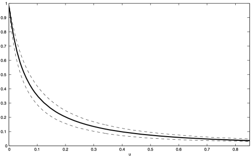
Figure 1: The solid line is the fitted parametric Laplace transform of the marginal distribution of the scale of the log VIX index, which essentially plots on top of the estimated realized Laplace transform (not visible), and the dashed lines show 95 percent nonparametric confidence intervals about the estimated realized Laplace transform.

6 Conclusion

We derive the asymptotic properties of the realized Laplace transform for pure-jump processes computed from high-frequency data. The realized Laplace transform is shown to estimate the Laplace transform of the stochastic scale of the observed process. The results are (locally) uniform over the argument of the transform. We can thereby also derive the asymptotic properties of parameter estimates obtained by fitting parametric models for the marginal law of the stochastic scale to the realized Laplace transform. This estimation entails minimizing a measure of the discrepancy between between the model-implied and observed transforms.

7 Proofs

Here we give the proof of the main results in the paper: Lemma 1 and Theorems 1 and 3, with the rest relegated in the supplementary Appendix. In all the proofs we will denote with $C$ a constant that does not depend on $T$ and $\Delta_{n}$, and further it might change from line to line. We also use the shorthand $\mathbb{E}_{i-1}^{n}$ for $\mathbb{E}(\cdot|\mathscr{F}_{(i-1)\Delta_{n}})$. We start with stating some preliminary results, proofs of which are in the supplement, and which we use in the proofs of the theorems.

7.1 Preliminary results

For a symmetric stable process with Lévy measure $\frac{c}{|x|^{\beta+1}}\,dx$ for some $c>0$ and $\beta\in(1,2)$, using Theorems 14.5 and 14.7 of SATO , we can write its characteristic function at time $1$ as

$$\exp\biggl{(}c\int_{0}^{\infty}(e^{iur}-1-iur)\frac{dr}{r^{1+\beta}}+c\int_{0}^{\infty}(e^{-iur}-1+iur)\frac{dr}{r^{1+\beta}}\biggr{)},\qquad u\in\mathbb{R}.$$

Then using Lemma 14.11 of SATO , we can simplify the above expression to

$$\exp\bigl{(}2c\Gamma(-\beta)\cos(\beta\pi/2)|u|^{\beta}\bigr{)},$$

where $\Gamma(-\beta)=\frac{\Gamma(2-\beta)}{\beta(\beta-1)}$ for $\beta\in(1,2)$. Therefore, the Lévy measure of a $\beta$-stable process, $L_{t}$, with $\mathbb{E}(e^{-iuL_{t}})=e^{-t|u|^{\beta}/2}$, is

$$A\times\frac{1}{|x|^{\beta+1}}\,dx,$$

for $A$ defined in (4). Throughout, after appropriately extending the original probability space, we will use the following alternative representation of the process $X_{t}$ (proof of which is given in the supplement):

$$X_{t} = X_{0}+\int_{0}^{t}\overline{\alpha}_{s}\,ds+\int_{0}^{t}\int_{\mathbb{R}}\sigma_{s-}x\tilde{\mu}_{1}(ds,dx)$$

$${}+\int_{0}^{t}\int_{\mathbb{R}}\sigma_{s-}x\mu_{2}(ds,dx)-\int_{0}^{t}\int_{\mathbb{R}}\sigma_{s-}x\mu_{3}(ds,dx)+Y_{t},$$

where $\mu_{1}$, $\mu_{2}$ and $\mu_{3}$ are homogenous Poisson measures (the three measures are not mutually independent), with compensators, respectively, $\nu_{1}(dx)=\frac{A}{|x|^{\beta+1}}\,dx$, $\nu_{2}(dx)=|\nu^{\prime}(x)|\,dx$ and $\nu_{3}(dx)=2|\nu^{\prime}(x)|1(\nu^{\prime}(x)<0)\,dx$ and $\overline{\alpha}_{s}=\alpha_{s}-\sigma_{s-}\int_{\mathbb{R}}x\nu^{\prime}(x)\,dx$. Finally, to simplify notation we will also use the shorthand $L_{t}=\int_{0}^{t}\int_{\mathbb{R}}x\tilde{\mu}_{1}(ds,dx)$ and further for a symmetric bounded function $\kappa$ with $\kappa(x)=x$ for $x$ in a neighborhood of zero, we decompose

$$L_{t}=\overline{L}_{t}+\widetilde{L}_{t},$$

$$\eqntext{\displaystyle\overline{L}_{t}=\int_{0}^{t}\int_{\mathbb{R}}\bigl{(}x-\kappa(x)\bigr{)}\tilde{\mu}_{1}(ds,dx),\qquad\widetilde{L}_{t}=\int_{0}^{t}\int_{\mathbb{R}}\kappa(x)\tilde{\mu}_{1}(ds,dx).}$$ (35)

With this notation we make the following decomposition:

$$V_{T}(X,\Delta_{n},\beta,u)-\int_{0}^{T}e^{-u|\sigma_{t}|^{\beta}}\,dt$$

(36)

$$\qquad=\sum_{i=1}^{[T/\Delta_{n}]}\sum_{j=1}^{3}\xi_{i,u}^{(j)}+\int_{[T/\Delta_{n}]\Delta_{n}}^{T}e^{-u|\sigma_{t}|^{\beta}}\,dt,$$

$$\xi_{i,u}^{(1)} = \Delta_{n}\cos\bigl{(}(2u)^{1/\beta}\sigma_{(i-1)\Delta_{n}-}\Delta_{n}^{-1/\beta}\Delta_{i}^{n}L\bigr{)}-\int_{(i-1)\Delta_{n}}^{i\Delta_{n}}e^{-u|\sigma_{(i-1)\Delta_{n}-}|^{\beta}}\,ds,$$

$$\xi_{i,u}^{(2)} = \int_{(i-1)\Delta_{n}}^{i\Delta_{n}}\bigl{(}e^{-u|\sigma_{(i-1)\Delta_{n}-}|^{\beta}}-e^{-u|\sigma_{s}|^{\beta}}\bigr{)}\,ds,$$

$$\xi_{i,u}^{(3)} = \Delta_{n}\bigl{(}\cos((2u)^{1/\beta}\Delta_{n}^{-1/\beta}\Delta_{i}^{n}X)-\cos\bigl{(}(2u)^{1/\beta}\sigma_{(i-1)\Delta_{n}-}\Delta_{n}^{-1/\beta}\Delta_{i}^{n}L\bigr{)}\bigr{)}.$$

Starting with $\xi_{i,u}^{(1)}$, using the self-similarity of the stable process $L_{t}$, and the expression for its characteristic function, we have

$$\qquad\cases{\mathbb{E}_{i-1}^{n}\bigl{(}\cos\bigl{(}(2u)^{1/\beta}\sigma_{(i-1)\Delta_{n}-}\Delta_{n}^{-1/\beta}\Delta_{i}^{n}L\bigr{)}-e^{-u|\sigma_{(i-1)\Delta_{n}-}|^{\beta}}\bigr{)}=0,\cr\mathbb{E}_{i-1}^{n}\bigl{(}\cos\bigl{(}(2u)^{1/\beta}\sigma_{(i-1)\Delta_{n}-}\Delta_{n}^{-1/\beta}\Delta_{i}^{n}L\bigr{)}-e^{-u|\sigma_{(i-1)\Delta_{n}-}|^{\beta}}\bigr{)}^{2}\cr\qquad=F_{\beta}\bigl{(}u^{1/\beta}\bigl{|}\sigma_{(i-1)\Delta_{n}-}\bigr{|}\bigr{)},\cr\mathbb{E}_{i-1}^{n}\bigl{(}\cos\bigl{(}(2u)^{1/\beta}\sigma_{(i-1)\Delta_{n}-}\Delta_{n}^{-1/\beta}\Delta_{i}^{n}L\bigr{)}-e^{-u|\sigma_{(i-1)\Delta_{n}-}|^{\beta}}\bigr{)}^{4}\leq C.}$$ (37)

Using first-order Taylor expansion we decompose $\xi_{i,u}^{(2)}=\sum_{j=1}^{3}\xi_{i,u}^{(2)}(j)$ where

$$\xi_{i,u}^{(2)}(1) = \Upsilon\bigl{(}\sigma_{(i-1)\Delta_{n}-},u\bigr{)}$$

$${}\times\int_{(i-1)\Delta_{n}}^{i\Delta_{n}}\biggl{(}\int_{(i-1)\Delta_{n}}^{s}\tilde{\sigma}_{u}\,dW_{u}+\int_{(i-1)\Delta_{n}}^{s}\int_{\mathbb{R}}\underline{\delta}(u-,x)\tilde{\underline{\mu}}(du,dx)\biggr{)}\,ds,$$

$$\xi_{i,u}^{(2)}(2) = \int_{(i-1)\Delta_{n}}^{i\Delta_{n}}\bigl{(}\Upsilon(\sigma_{s}^{*},u)-\Upsilon\bigl{(}\sigma_{(i-1)\Delta_{n}-,u}\bigr{)}\bigr{)}$$

$${}\times\biggl{(}\int_{(i-1)\Delta_{n}}^{s}\tilde{\sigma}_{u}\,dW_{u}+\int_{(i-1)\Delta_{n}}^{s}\int_{\mathbb{R}^{2}}\underline{\delta}(u-,x)\tilde{\underline{\mu}}(du,dx)\biggr{)}\,ds,$$

$$\xi_{i,u}^{(2)}(3) = \int_{(i-1)\Delta_{n}}^{i\Delta_{n}}\bigl{(}e^{-u|\widehat{\sigma}_{s}|^{\beta}}-e^{-u|\sigma_{s}|^{\beta}}\bigr{)}\,ds,$$

where $\Upsilon(x,u)=\beta\operatorname{sign}\{x\}u|x|^{\beta-1}e^{-u|x|^{\beta}}$, $\sigma_{s}^{*}$ is a number between $\sigma_{(i-1)\Delta_{n}-}$ and $\widehat{\sigma}_{s}$, and

$$\widehat{\sigma}_{s}=\sigma_{(i-1)\Delta_{n}-}+\int_{(i-1)\Delta_{n}}^{s}\tilde{\sigma}_{u}\,dW_{u}+\int_{(i-1)\Delta_{n}}^{s}\int_{\mathbb{R}}\underline{\delta}(u-,x)\tilde{\underline{\mu}}(du,dx),$$

$$\eqntext{s\in[(i-1)\Delta_{n},i\Delta_{n}].}$$ (38)

We derive the following bounds in the supplement for any finite $\overline{u}>0$

$$\sum_{i=1}^{[T/\Delta_{n}]}\mathbb{E}_{i-1}^{n}\bigl{(}\xi_{i,u}^{(2)}(1)\bigr{)} = 0,$$

$$\frac{\Delta_{n}^{-2}}{T}\mathbb{E}\Biggl{(}\sum_{i=1}^{[T/\Delta_{n}]}\mathbb{E}_{i-1}^{n}\bigl{(}\xi_{i,u}^{(2)}(1)\bigr{)}^{2}\Biggr{)} \leq C,$$

$$(T\Delta_{n}^{\beta/2})^{-1}\sum_{i=1}^{[T/\Delta_{n}]}\mathbb{E}\Bigl{(}\sup_{0\leq u\leq\overline{u}}\bigl{|}\xi_{i,u}^{(2)}(2)\bigr{|}\Bigr{)} \leq C,$$ (40)

$$(T\Delta_{n})^{-1}\sum_{i=1}^{[T/\Delta_{n}]}\mathbb{E}\Bigl{(}\sup_{0\leq u\leq\overline{u}}\bigl{|}\xi_{i,u}^{(2)}(3)\bigr{|}\Bigr{)} \leq C.$$ (41)

Turning to $\xi_{i,u}^{(3)}$, we can first make the following decomposition [recall the decomposition of $L_{t}$ in (7.1)]:

$$\cos(\chi_{1})-\cos(\chi_{5})=\sum_{j=1}^{4}[\cos(\chi_{j})-\cos(\chi_{j+1})],$$ (42)

$$\chi_{1} = (2u)^{1/\beta}\Delta_{n}^{-1/\beta}\Delta_{i}^{n}X,$$

$$\chi_{2} = (2u)^{1/\beta}\Delta_{n}^{-1/\beta}\biggl{(}\int_{(i-1)\Delta_{n}}^{i\Delta_{n}}\overline{\alpha}_{s}\,ds+\int_{(i-1)\Delta_{n}}^{i\Delta_{n}}\sigma_{s-}\,dL_{s}\biggr{)},$$

$$\chi_{3} = (2u)^{1/\beta}\Delta_{n}^{-1/\beta}\biggl{(}\Delta_{n}\overline{\alpha}_{(i-1)\Delta_{n}}+\int_{(i-1)\Delta_{n}}^{i\Delta_{n}}\sigma_{s-}\,d\widetilde{L}_{s}\biggr{)},$$

$$\chi_{4} = (2u)^{1/\beta}\Delta_{n}^{-1/\beta}\sigma_{(i-1)\Delta_{n}-}\Delta_{i}^{n}\widetilde{L},$$

$$\chi_{5} = (2u)^{1/\beta}\Delta_{n}^{-1/\beta}\sigma_{(i-1)\Delta_{n}-}\Delta_{i}^{n}L.$$

Then, using the formula for $\cos(x)-\cos(y)$, $x,y\in\mathbb{R}$ for the first bracketed term on the right-hand side of (42) and a second-order Taylor expansion for the third one, allows us to write $\xi_{i,u}^{(3)}=\sum_{j=1}^{5}\xi_{i,u}^{(3)}(j)$ where

$$\xi_{i,u}^{(3)}(1) = -2\Delta_{n}$$

$${}\times\sin\biggl{(}0.5(2u)^{1/\beta}\Delta_{n}^{-1/\beta}\biggl{(}\Delta_{i}^{n}X+\int_{(i-1)\Delta_{n}}^{i\Delta_{n}}\overline{\alpha}_{s}\,ds+\int_{(i-1)\Delta_{n}}^{i\Delta_{n}}\sigma_{s-}\,dL_{s}\biggr{)}\biggr{)}$$

$${}\times\sin\biggl{(}0.5(2u)^{1/\beta}\Delta_{n}^{-1/\beta}\biggl{(}\Delta_{i}^{n}X-\int_{(i-1)\Delta_{n}}^{i\Delta_{n}}\overline{\alpha}_{s}\,ds-\int_{(i-1)\Delta_{n}}^{i\Delta_{n}}\sigma_{s-}\,dL_{s}\biggr{)}\biggr{)},$$

$$\xi_{i,u}^{(3)}(2) = -(2u)^{1/\beta}\Delta_{n}^{2-1/\beta}\sin\bigl{(}(2u)^{1/\beta}\sigma_{(i-1)\Delta_{n}-}\Delta_{n}^{-1/\beta}\Delta_{i}^{n}\widetilde{L}\bigr{)}\overline{\alpha}_{(i-1)\Delta_{n}},$$

$$\xi_{i,u}^{(3)}(3) = -(2u)^{1/\beta}\Delta_{n}^{1-1/\beta}\sin\bigl{(}(2u)^{1/\beta}\sigma_{(i-1)\Delta_{n}-}\Delta_{n}^{-1/\beta}\Delta_{i}^{n}\widetilde{L}\bigr{)}$$

$${}\times\int_{(i-1)\Delta_{n}}^{i\Delta_{n}}\bigl{(}\sigma_{s-}-\sigma_{(i-1)\Delta_{n}-}\bigr{)}\,d\widetilde{L}_{s},$$

$$\xi_{i,u}^{(3)}(4) = \Delta_{n}[\cos(\chi_{2})-\cos(\chi_{3})]+\Delta_{n}[\cos(\chi_{4})-\cos(\chi_{5})],$$

$$\xi_{i,u}^{(3)}(5) = 0.5(2u)^{2/\beta}\Delta_{n}^{1-2/\beta}$$

$${}\times\cos(\tilde{\chi})\biggl{(}\Delta_{n}\overline{\alpha}_{(i-1)\Delta_{n}}+\int_{(i-1)\Delta_{n}}^{i\Delta_{n}}\bigl{(}\sigma_{s-}-\sigma_{(i-1)\Delta_{n}-}\bigr{)}\,d\widetilde{L}_{s}\biggr{)}^{2},$$

with $\tilde{\chi}$ denoting some value between $\chi_{3}$ and $\chi_{4}$.

We derive the following bounds in the supplement for any finite $\overline{u}>0$:

$$\hskip 10.0pt\displaystyle(T|\log(\Delta_{n})|\Delta_{n}^{1-\beta^{\prime}/\beta})^{-1}\sum_{i=1}^{[T/\Delta_{n}]}\mathbb{E}\Bigl{(}\sup_{0\leq u\leq\overline{u}}\bigl{|}\xi_{i,u}^{(3)}(1)\bigr{|}\Bigr{)}\leq C,$$ (43)

$$\hskip 10.0pt\displaystyle\mathbb{E}_{i-1}^{n}\Bigl{(}\xi_{i,u}^{(3)}(2)\Bigr{)}=0,\qquad\frac{(\Delta_{n}^{3-2/\beta})^{-1}}{T}\mathbb{E}\Biggl{(}\sum_{i=1}^{[T/\Delta_{n}]}\mathbb{E}_{i-1}^{n}\bigl{(}\xi_{i,u}^{(3)}(2)\bigr{)}^{2}\Biggr{)}\leq C,$$ (44)

$$\hskip 10.0pt\displaystyle(T\Delta_{n}^{3/2-1/\beta})^{-1}\sum_{i=1}^{[T/\Delta_{n}]}\mathbb{E}\Bigl{(}\sup_{0\leq u\leq\overline{u}}\bigl{|}\xi_{i,u}^{(3)}(4)\bigr{|}\Bigr{)}\leq C,$$ (45)

$$\hskip 10.0pt\displaystyle(T\Delta_{n}^{2-2/\beta})^{-1}\sum_{i=1}^{[T/\Delta_{n}]}\mathbb{E}\Bigl{(}\sup_{0\leq u\leq\overline{u}}\bigl{|}\xi_{i,u}^{(3)}(5)\bigr{|}\Bigr{)}\leq C,$$ (46)

$$\hskip 10.0pt\displaystyle(T\Delta_{n}^{1-\iota})^{-1}\mathbb{E}\Biggl{(}\sup_{0\leq u\leq\overline{u}}\Biggl{|}\sum_{i=1}^{[T/\Delta_{n}]}\mathbb{E}_{i-1}^{n}\xi_{i,u}^{(3)}(3)\Biggr{|}\Biggr{)}\leq C$$ (47)

$$\eqntext{\mbox{under Assumption~{}\ref{assb1}},}$$ (48)

$$\hskip 10.0pt\displaystyle\bigl{(}T\Delta_{n}^{1/(\beta\vee\beta^{{}^{\prime\prime}}+\iota)}\bigr{)}^{-1}\mathbb{E}\Biggl{(}\sup_{0\leq u\leq\overline{u}}\Biggl{|}\sum_{i=1}^{[T/\Delta_{n}]}\mathbb{E}_{i-1}^{n}\xi_{i,u}^{(3)}(3)\Biggr{|}\Biggr{)}\leq C$$ (49)

$$\eqntext{\mbox{under Assumption~{}\ref{assb}},}$$ (50)

$$\hskip 10.0pt\displaystyle(T\Delta_{n}^{3-2/\beta})^{-1}\sum_{i=1}^{[T/\Delta_{n}]}\mathbb{E}\Bigl{(}\sup_{0\leq u\leq\overline{u}}\bigl{|}\xi_{i,u}^{(3)}(3)\bigr{|}^{2}\Bigr{)}\leq C.$$ (51)

7.2 Proof of Lemma 1

Since $h^{-1/\beta}Z_{ht}$ is a Lévy process, to prove the convergence of the sequence, we need to show the convergence of its characteristics (see, e.g., JS , Corollary VII.3.6); that is, we need to establish the following for $h\rightarrow 0$:

$$\cases{\displaystyle h^{1-2/\beta}\int_{\mathbb{R}}\kappa^{2}(h^{-1/\beta}x)\nu(x)\,dx\longrightarrow\int_{\mathbb{R}}\kappa^{2}(x)\frac{A}{|x|^{\beta+1}}\,dx,\cr\displaystyle h\int_{\mathbb{R}}g(h^{-1/\beta}x)\nu(x)\,dx\longrightarrow\int_{\mathbb{R}}g(x)\frac{A}{|x|^{\beta+1}}\,dx,}$$ (52)

where $g$ is an arbitrary continuous and bounded function on $\mathbb{R}$, which is $0$ around $0$.

The result in (52) follows by a change of variable in the integration, and by using the fact that by Assumption A we have $|\nu^{\prime}(x)|<\frac{C}{|x|^{\beta^{\prime}+1}}$ for $|x|\leq x_{0}$ where $x_{0}$ is fixed and $\beta^{\prime}<\beta$.

7.3 Proof of Theorem 1

Part (b) of the theorem holds from the bounds in (37)–(41) and (43)–(51), so we are left with showing part (a). First, we show that for $\Delta_{n}\rightarrow 0$, $\frac{1}{\sqrt{\Delta_{n}}}\sum_{i=1}^{[t/\Delta_{n}]}\xi_{i,u}^{(1)}$ converges stably as a process in $t$ for the Skorokhod topology to the process $\int_{0}^{t}\sqrt{F_{\beta}(u^{1/\beta}|\sigma_{s}|)}\,dW_{s}^{\prime}$, where $W_{t}^{\prime}$ is a Brownian motion defined on an extension of the original probability space and is independent from the $\sigma$-field $\mathcal{F}$. Using the result in (37), we get for every $t>0$,

$$\cases{\displaystyle\frac{1}{\sqrt{\Delta_{n}}}\sum_{i=1}^{[t/\Delta_{n}]}\mathbb{E}_{i-1}^{n}\bigl{(}\xi_{i,u}^{(1)}\bigr{)}\stackrel{{\scriptstyle\mathbb{P}}}{{\longrightarrow}}0,\vspace*{3pt}\cr\displaystyle\frac{1}{\Delta_{n}}\sum_{i=1}^{[t/\Delta_{n}]}\mathbb{E}_{i-1}^{n}\bigl{(}\xi_{i,u}^{(1)}\bigr{)}^{2}\stackrel{{\scriptstyle\mathbb{P}}}{{\longrightarrow}}\int_{0}^{t}F_{\beta}(u^{1/\beta}|\sigma_{s}|)\,ds,\vspace*{3pt}\cr\displaystyle\frac{1}{\Delta_{n}^{2}}\sum_{i=1}^{[t/\Delta_{n}]}\mathbb{E}_{i-1}^{n}\bigl{(}\xi_{i,u}^{(1)}\bigr{)}^{4}\stackrel{{\scriptstyle\mathbb{P}}}{{\longrightarrow}}0,}$$

where for the second convergence above, we made use of Riemann integrability. Thus to show the stable convergence, given the above result and upon using Theorem IX.7.28 of JS , we need to show only

$$\sum_{i=1}^{[t/\Delta_{n}]}\mathbb{E}_{i-1}^{n}\bigl{(}\sqrt{1/\Delta_{n}}\xi_{i,u}^{(1)}\Delta_{i}^{n}M\bigr{)}\stackrel{{\scriptstyle\mathbb{P}}}{{\longrightarrow}}0\qquad\forall t>0,$$ (53)

where $M$ is a bounded martingale defined on the original probability space.

When $M$ is discontinuous martingale, we can argue as follows. First, we can set $M_{t}^{n}=M_{[t/\Delta_{n}]\Delta_{n}}$ and $N_{t}^{n}=\sum_{i=1}^{[t/\Delta_{n}]}\sqrt{1/\Delta_{n}}\xi_{i,u}^{(1)}$ for any $t$. With this notation we have $[M^{n},N^{n}]_{t}=\sum_{i=1}^{[t/\Delta_{n}]}(\sqrt{1/\Delta_{n}}\xi_{i,u}^{(1)}\Delta_{i}^{n}M)$ and $\langle M^{n},N^{n}\rangle_{t}=\sum_{i=1}^{[t/\Delta_{n}]}\mathbb{E}_{i-1}^{n}(\sqrt{1/\Delta_{n}}\xi_{i,u}^{(1)}\Delta_{i}^{n}M)$. We trivially have that $M^{n}$ converges (for the Skorokhod topology) to $M$, and furthermore from the results above the limit of $N^{n}$, which we denote here with $N$, is a continuous process. Therefore, using Corollary VI.3.33(b) of JS , we have that $(M^{n},N^{n})$ is tight. Then, using the fact that $M$ is a bounded martingale (and hence it has bounded jumps), we can apply Corollary VI.6.29 of JS and conclude that the limit of $[M^{n},N^{n}]$ (up to taking a subsequence) is $[M,N]$. However, since continuous and pure-jump martingales are orthogonal (see, e.g., Definition I.4.11 of JS ), we conclude that $[M,N]=0$. Further, the difference $[M^{n},N^{n}]-\langle M^{n},N^{n}\rangle$ is a martingale, and using Itô isometry, the fact that $\sqrt{1/\Delta_{n}}\xi_{i,u}^{(1)}\leq C\sqrt{\Delta_{n}}$, and the boundedness of $M$, we have

$$\mathbb{E}([M^{n},N^{n}]_{t}-\langle M^{n},N^{n}\rangle_{t})^{2} = \mathbb{E}\biggl{(}\sum_{s\leq t}(\Delta M_{s}^{n}\Delta N_{s}^{n})^{2}\biggr{)}$$

$$\leq C\Delta_{n}\mathbb{E}\biggl{(}\sum_{s\leq t}(\Delta M_{s}^{n})^{2}\biggr{)}\leq C\Delta_{n}.$$

Therefore, $[M^{n},N^{n}]-\langle M^{n},N^{n}\rangle$ converges in probability to zero, and hence so does $\langle M^{n},N^{n}\rangle$.

When $M$ is a continuous martingale, we can write $\mathbb{E}_{i-1}^{n}(\xi_{i,u}^{(1)}\Delta_{i}^{n}M)=\mathbb{E}_{i-1}^{n}(\Delta_{i}^{n}N\Delta_{i}^{n}M)$ where now we denote $N_{t}=\mathbb{E}(\xi_{i,u}^{(1)}|\mathscr{F}_{t})$ for $t\in[(i-1)\Delta_{n},i\Delta_{n}]$ (which is obviously a martingale with respect to the filtration $\mathscr{F}_{t}$). However, note that $\xi_{i,u}^{(1)}$ is uniquely determined by $\mathscr{F}_{(i-1)\Delta_{n}}$ and the homogenous Poisson measure $\mu_{1}$. Therefore, $N_{t}$ remains a martingale for the coarser filtration $\mathscr{F}^{*}_{t}=\mathscr{F}_{(i-1)\Delta_{n}}\cap\mathscr{F}_{t}^{\mu_{1}}$ for $\mathscr{F}_{t}^{\mu_{1}}$ being the filtration generated by the jump measure $\mu_{1}$. Then using a martingale representation for the martingale $(N_{t})_{t\geq(i-1)\Delta_{n}}$ with respect to the filtration $\mathscr{F}^{*}_{t}$ (note $\mu_{1}$ is a homogenous Poisson measure), Theorem III.4.34 of JS , we can represent $N_{t}$ as a sum of $\mathscr{F}_{(i-1)\Delta_{n}}$-adapted variable and an integral, with respect to $\tilde{\mu}_{1}$. But then since pure-jump and continuous martingales are orthogonal, we have $\mathbb{E}_{i-1}^{n}(\xi_{i,u}^{(1)}\Delta_{i}^{n}M)=0$.

This establishes the stable convergence of $\frac{1}{\sqrt{\Delta_{n}}}\sum_{i=1}^{[t/\Delta_{n}]}\xi_{i,u}^{(1)}$. Next, the bounds for $\xi_{i,u}^{(2)}$ and $\xi_{i,u}^{(3)}$ in (7.1)–(41) and (43)–(46) imply that$\frac{1}{\sqrt{\Delta_{n}}}\sum_{i=1}^{[T/\Delta_{n}]}(\xi_{i,u}^{(2)}+\xi_{i,u}^{(3)})$ is asymptotically negligible for $\Delta_{n}\rightarrow 0$, and $T$ fixed.

7.4 Proof of Theorem 3

Part (a). The proof consists of showing finite-dimensional convergence in $u$ and tightness of the sequence:

(1) Finite-dimensional convergence. First, given Assumption C, and using a CLT for stationary and ergodic process (see JS , Theorem VIII.3.79), we have for a finite-dimensional vector $\mathbf{u}$,

$$\sqrt{T}\biggl{(}\frac{1}{T}\int_{0}^{T}e^{-\mathbf{u}|\sigma_{t}|^{\beta}}\,dt-\mathcal{L}_{\beta}(\mathbf{u})\biggr{)}\stackrel{{\scriptstyle\mathcal{L}}}{{\longrightarrow}}\Psi,$$ (54)

where $\Psi$ is a zero-mean normal variable with elements of the variance–covariance matrix given by $\Sigma_{\beta}(u_{i},u_{j})$.

Next, the results in Section 7.1 imply for $T\rightarrow\infty$ and $\Delta_{n}\rightarrow 0$ under the weaker Assumption B.

$$\hskip 35.0pt\frac{1}{\sqrt{T}}\sum_{i=1}^{[T/\Delta_{n}]}\xi_{i,u}^{(1)} = o_{p}\bigl{(}\sqrt{\Delta_{n}}\bigr{)},\qquad\frac{1}{\sqrt{T}}\sum_{i=1}^{[T/\Delta_{n}]}\xi_{i,u}^{(2)}=o_{p}\bigl{(}\sqrt{T}\Delta_{n}^{\beta/2}\vee\sqrt{\Delta_{n}}\bigr{)},$$

$$\hskip 35.0pt\frac{1}{\sqrt{T}}\sum_{i=1}^{[T/\Delta_{n}]}\xi_{i,u}^{(3)} = o_{p}\bigl{(}\sqrt{T}\bigl{(}|\log(\Delta_{n})|\Delta_{n}^{1-\beta^{\prime}/\beta}\vee\Delta_{n}^{(2-2/\beta)\wedge 1/2}\bigr{)}\vee\sqrt{\Delta_{n}}\bigr{)},$$

with the last one replaced with the weaker

$$\frac{1}{\sqrt{T}}\sum_{i=1}^{[T/\Delta_{n}]}\xi_{i,u}^{(3)}=o_{p}\bigl{(}\sqrt{T}\bigl{(}|\log(\Delta_{n})|\Delta_{n}^{1-\beta^{\prime}/\beta}\vee\Delta_{n}^{2-2/\beta}\bigr{)}\vee\sqrt{\Delta_{n}}\bigr{)},$$

when the stronger Assumption B^′ holds.

(2) Tightness. Let’s denote for arbitrary $u,v\geq 0$,

$$z_{t}=\bigl{(}e^{-u|\sigma_{t}|^{\beta}}-\mathcal{L}_{\beta}(u)\bigr{)}-\bigl{(}e^{-v|\sigma_{t}|^{\beta}}-\mathcal{L}_{\beta}(v)\bigr{)}.$$

Then, using successive conditioning and Lemma VIII.3.102 in JS , together with the boundedness of $z_{t}$ and Assumption C, we get

$$\mathbb{E}\Biggl{(}\frac{1}{\sqrt{T}}\sum_{t=1}^{T}z_{t}\,dt\Biggr{)}^{2} = \frac{1}{T}\int_{0}^{T}\int_{0}^{T}\mathbb{E}(z_{t}z_{s})\,ds\,dt$$

$$\leq C|u^{1/p}-v^{1/p}|\frac{1}{T}\int_{0}^{T}\int_{0}^{T}\mathbb{E}(|\sigma_{s\wedge t}|^{\beta/p}\mathbb{E}(z_{s\vee t}|\mathscr{F}_{s\wedge t}))\,ds\,dt$$

$$\leq C|u^{1/p}-v^{1/p}|^{1+\iota}\frac{1}{T}\int_{0}^{T}\int_{0}^{T}\bigl{(}\alpha_{|t-s|}^{\mathrm{mix}}\bigr{)}^{1/3-\iota}\,dt\,ds$$

$$\leq C|u^{1/p}-v^{1/p}|^{1+\iota}\int_{0}^{\infty}(\alpha_{s}^{\mathrm{mix}})^{1/3-\iota}\,ds\leq C|u^{1/p}-v^{1/p}|^{1+\iota},$$

where $\iota>0$ is the constant of Assumption C and $p>3$. Using Theorem 12.3 of Billingsley , the above bound implies the tightness of the sequence $\frac{1}{\sqrt{T}}\int_{0}^{T}(e^{-u|\sigma_{t}|^{\beta}}-\mathcal{L}_{\beta}(u))\,dt$, and from here we have its convergence for the local uniform topology.

Turning now to $\frac{1}{\sqrt{\Delta_{n}}}\sum_{i=1}^{[T/\Delta_{n}]}\xi_{i,u}^{(1)}$, we can use the analog of the result in (37) for $\xi_{i,u}^{(1)}-\xi_{i,v}^{(1)}$, to get

$$\mathbb{E}\Biggl{(}\frac{1}{\sqrt{T\Delta_{n}}}\sum_{i=1}^{[T/\Delta_{n}]}\bigl{(}\xi_{i,u}^{(1)}-\xi_{i,v}^{(1)}\bigr{)}\Biggr{)}^{2}\leq C|u^{1/\beta}-v^{1/\beta}|^{2},$$

for some constant $C$. From here, using Theorem 12.3 of Billingsley , we get the tightness of $\frac{1}{\sqrt{T\Delta_{n}}}\sum_{i=1}^{[T/\Delta_{n}]}\xi_{i,u}^{(1)}$.

Similarly, using the analog of (44) applied to $\xi_{i,u}^{(3)}(2)-\xi_{i,v}^{(3)}(2)$, we have

$$\qquad\frac{\Delta_{n}^{-(3-2/\beta)}}{T}\mathbb{E}\Biggl{(}\sum_{i=1}^{[T/\Delta_{n}]}\bigl{(}\xi_{i,u}^{(3)}(2)-\xi_{i,v}^{(3)}(2)\bigr{)}\Biggr{)}^{2}\leq C|u^{1/\beta}-v^{1/\beta}|^{2}.$$ (56)

This establishes tightness for $\Delta_{n}^{-(3/2-1/\beta)}\sum_{i=1}^{[T/\Delta_{n}]}\xi_{i,u}^{(3)}(2)$. We can do exactly the same for $\Delta_{n}^{-(3/2-1/\beta)}\sum_{i=1}^{[T/\Delta_{n}]}(\xi_{i,u}^{(3)}(3)-\mathbb{E}_{i-1}^{n}(\xi_{i,u}^{(3)}(3)))$ using the analog of (51) applied to $\xi_{i,u}^{(3)}(3)-\xi_{i,v}^{(3)}(3)-\mathbb{E}_{i-1}^{n}(\xi_{i,u}^{(3)}(3)-\xi_{i,v}^{(3)}(3))$. Next,

$$\frac{\Delta_{n}^{-2}}{T}\mathbb{E}\Biggl{(}\sum_{i=1}^{[T/\Delta_{n}]}\bigl{(}\xi_{i,u}^{(2)}(1)-\xi_{i,v}^{(2)}(1)\bigr{)}\Biggr{)}^{2}\leq C(u-v)^{2},$$ (57)

where we used successive conditioning and further made use of the inequality

$$|\Upsilon(x,u)-\Upsilon(x,v)|\leq C|x|^{\beta-1}|u-v|,\qquad x\in\mathbb{R},u,v\geq 0,$$

which follows from applying first-order Taylor expansion of $\Upsilon(x,u)$ in its second argument and using the fact that the derivative of $\Upsilon(x,u)$ in its second argument is bounded by $C|x|^{\beta-1}$. Therefore, $\sum_{i=1}^{[T/\Delta_{n}]}\frac{\Delta_{n}^{-1}}{\sqrt{T}}\xi_{i,u}^{(2)}(1)$ is tight on the space of continuous functions equipped with the local uniform topology.

Next, using the results in Section 7.1, it is easy to show that for any finite $\overline{u}>0$, we have

$$\lim_{\Delta_{n}\downarrow 0,T\uparrow\infty}\mathbb{P}\Biggl{(}\sup_{0\leq u\leq\overline{u}}\Biggl{|}\sum_{i=1}^{[T/\Delta_{n}]}(T\Delta_{n}^{\beta/2})^{-1}\xi_{i,u}^{(2)}(2)\Biggr{|}>\varepsilon_{n}\Biggr{)}=0\qquad\forall\varepsilon_{n}\uparrow\infty.$$ (58)

The same holds when, in the above, we replace $(T\Delta_{n}^{\beta/2})^{-1}\xi_{i,u}^{(2)}(2)$ with either of the following terms: $(T\Delta_{n})^{-1}\xi_{i,u}^{(2)}(3)$, $(T|\log(\Delta_{n})|\Delta_{n}^{1-\beta^{\prime}/\beta})^{-1}\xi_{i,u}^{(3)}(1)$, $(T\Delta_{n}^{3/2-1/\beta})^{-1}\xi_{i,u}^{(3)}(4)$, $(T\Delta_{n}^{2-2/\beta})^{-1}\xi_{i,u}^{(3)}(5)$ as well as $(T\Delta_{n}^{{}^{1-\iota}})^{-1}\mathbb{E}_{i-1}^{n}(\xi_{i,u}^{(3)}(3))$ under Assumption B^′ and $(T\Delta_{n}^{1/(\beta\vee\beta^{{}^{\prime\prime}}+\iota)})^{-1}\mathbb{E}_{i-1}^{n}(\xi_{i,u}^{(3)}(3))$ under the weaker Assumption B. This implies that those terms are, uniformly in $u$, bounded in probability.

Part (b). First, (22) follows directly from Theorem 1, so here we only show (3). If we denote for $k\geq 0$,

$$C_{k,\beta}(u,v)=\frac{1}{T}\sum_{t=k+1}^{T}\int_{t-1}^{t}\bigl{(}e^{-u|\sigma_{s}|^{\beta}}-\mathcal{L}_{\beta}(u)\bigr{)}\,ds\int_{t-k-1}^{t-k}\bigl{(}e^{-v|\sigma_{s}|^{\beta}}-\mathcal{L}_{\beta}(v)\bigr{)}\,ds,$$

then under our assumptions, by standard arguments (see, e.g., Proposition 1 in Andrews91 ), we have

$$\qquad C_{0,\beta}(u,v)+\sum_{i=1}^{L_{T}}\omega(i,L_{T})\bigl{(}C_{i,\beta}(u,v)+C_{i,\beta}(v,u)\bigr{)}\stackrel{{\scriptstyle\mathbb{P}}}{{\longrightarrow}}\Sigma_{\beta}(u,v).$$ (59)

Therefore, we are left showing

$$\bigl{(}\widehat{C}_{0,\beta}(u,v)-C_{0,\beta}(u,v)\bigr{)}$$

$$\qquad{}+\sum_{i=1}^{L_{T}}\omega(i,L_{T})\bigl{(}\widehat{C}_{i,\beta}(u,v)+\widehat{C}_{i,\beta}(v,u)$$ (60)

$$\hskip 70.0pt\qquad{}-C_{i,\beta}(u,v)-C_{i,\beta}(v,u)\bigr{)}\stackrel{{\scriptstyle\mathbb{P}}}{{\longrightarrow}}0.$$

We note that for arbitrary $1\leq k\leq T$, we have

$$\Delta_{n}\sum_{i=[(k-1)/\Delta_{n}]+1}^{[k/\Delta_{n}]}\cos((2u)^{1/\beta}\Delta_{n}^{-1/\beta}\Delta_{i}^{n}X)\leq 1\quad\mbox{and}\quad\int_{k-1}^{k}e^{-u|\sigma_{s}|^{\beta}}\,ds\leq 1.$$

Hence, for $k=0,1,\ldots,L_{T}$, we have

$$|\widehat{C}_{k,\beta}(u,v)-C_{k,\beta}(u,v)| \leq \frac{1}{T}\sum_{t=1}^{T}\biggl{|}\widehat{Z}_{t,\beta}(u)-\int_{t-1}^{t}e^{-u|\sigma_{s}|^{\beta}}\,ds\biggr{|}$$

$${}+\frac{1}{T}\sum_{t=1}^{T}\biggl{|}\widehat{Z}_{t,\beta}(v)-\int_{t-1}^{t}e^{-v|\sigma_{s}|^{\beta}}\,ds\biggr{|}$$

$${}+|\widehat{\mathcal{L}}_{\beta}(u)-\mathcal{L}_{\beta}(u)|$$

$${}+|\widehat{\mathcal{L}}_{\beta}(v)-\mathcal{L}_{\beta}(v)|+O\biggl{(}\frac{k}{T}\biggr{)}.$$

First, using the CLT result in (54), and since $L_{T}/\sqrt{T}\rightarrow 0$, we have

$$\sum_{i=1}^{L_{T}}|\omega(i,L_{T})||\widehat{\mathcal{L}}_{\beta}(u)-\mathcal{L}_{\beta}(u)|\stackrel{{\scriptstyle\mathbb{P}}}{{\longrightarrow}}0\qquad\forall u>0.$$ (61)

Further, using the stationarity of the process $\sigma_{t}$ and the bounds on the moments of the terms $\xi_{i,u}^{(j)}$ derived in Section 7.1, we have for every $t\geq 1$,

$$\mathbb{E}\biggl{|}\widehat{Z}_{t,\beta}(u)-\int_{t-1}^{t}e^{-u|\sigma_{s}|^{\beta}}\,ds\biggr{|}\leq C\bigl{(}|\log\Delta_{n}|\Delta_{n}^{1-\beta^{\prime}/\beta}\vee\Delta_{n}^{(2-2/\beta)\wedge 1/2}\bigr{)}.$$

Therefore, using the relative speed condition between $L_{T}$ and $\Delta_{n}$ in the theorem, we have

$$\frac{\sum_{i=1}^{L_{T}}|\omega(i,L_{T})|}{T}\sum_{t=1}^{T}\mathbb{E}\biggl{|}\widehat{Z}_{t,\beta}(u)-\int_{t-1}^{t}e^{-u|\sigma_{s}|^{\beta}}\,ds\biggr{|}\longrightarrow 0\qquad\forall u>0.$$ (62)

(61) and (62) imply (7.4), and this, combined with (59), establishes the result in (3).

References

• (1) {barticle}[mr] \bauthor\bsnmAït-Sahalia, \bfnmYacine\binitsY. and \bauthor\bsnmJacob, \bfnmJean\binitsJ. (\byear2007). \btitleVolatility estimators for discretely sampled Lévy processes. \bjournalAnn. Statist. \bvolume35 \bpages355–392. \biddoi=10.1214/009053606000001190, issn=0090-5364, mr=2332279 \bptokimsref \endbibitem
• (2) {barticle}[mr] \bauthor\bsnmAït-Sahalia, \bfnmYacine\binitsY. and \bauthor\bsnmJacod, \bfnmJean\binitsJ. (\byear2009). \btitleEstimating the degree of activity of jumps in high frequency data. \bjournalAnn. Statist. \bvolume37 \bpages2202–2244. \biddoi=10.1214/08-AOS640, issn=0090-5364, mr=2543690 \bptokimsref \endbibitem
• (3) {barticle}[mr] \bauthor\bsnmAndrews, \bfnmBeth\binitsB., \bauthor\bsnmCalder, \bfnmMatthew\binitsM. and \bauthor\bsnmDavis, \bfnmRichard A.\binitsR. A. (\byear2009). \btitleMaximum likelihood estimation for $\alpha$-stable autoregressive processes. \bjournalAnn. Statist. \bvolume37 \bpages1946–1982. \biddoi=10.1214/08-AOS632, issn=0090-5364, mr=2533476 \bptokimsref \endbibitem
• (4) {barticle}[mr] \bauthor\bsnmAndrews, \bfnmDonald W. K.\binitsD. W. K. (\byear1991). \btitleHeteroskedasticity and autocorrelation consistent covariance matrix estimation. \bjournalEconometrica \bvolume59 \bpages817–858. \biddoi=10.2307/2938229, issn=0012-9682, mr=1106513 \bptokimsref \endbibitem
• (5) {barticle}[mr] \bauthor\bsnmBarndorff-Nielsen, \bfnmOle E.\binitsO. E. and \bauthor\bsnmShephard, \bfnmNeil\binitsN. (\byear2001). \btitleNon-Gaussian Ornstein–Uhlenbeck-based models and some of their uses in financial economics. \bjournalJ. R. Stat. Soc. Ser. B Stat. Methodol. \bvolume63 \bpages167–241. \biddoi=10.1111/1467-9868.00282, issn=1369-7412, mr=1841412 \bptokimsref \endbibitem
• (6) {barticle}[mr] \bauthor\bsnmBelomestny, \bfnmDenis\binitsD. (\byear2010). \btitleSpectral estimation of the fractional order of a Lévy process. \bjournalAnn. Statist. \bvolume38 \bpages317–351. \biddoi=10.1214/09-AOS715, issn=0090-5364, mr=2589324 \bptokimsref \endbibitem
• (7) {barticle}[mr] \bauthor\bsnmBelomestny, \bfnmDenis\binitsD. (\byear2011). \btitleStatistical inference for time-changed Lévy processes via composite characteristic function estimation. \bjournalAnn. Statist. \bvolume39 \bpages2205–2242. \biddoi=10.1214/11-AOS901, issn=0090-5364, mr=2893866 \bptokimsref \endbibitem
• (8) {bbook}[mr] \bauthor\bsnmBillingsley, \bfnmPatrick\binitsP. (\byear1968). \btitleConvergence of Probability Measures. \bpublisherWiley, \baddressNew York. \bidmr=0233396 \bptokimsref \endbibitem
• (9) {barticle}[mr] \bauthor\bsnmBoyarchenko, \bfnmSvetlana\binitsS. and \bauthor\bsnmLevendorskiĭ, \bfnmSergei\binitsS. (\byear2002). \btitleBarrier options and touch-and-out options under regular Lévy processes of exponential type. \bjournalAnn. Appl. Probab. \bvolume12 \bpages1261–1298. \biddoi=10.1214/aoap/1037125863, issn=1050-5164, mr=1936593 \bptokimsref \endbibitem
• (10) {bincollection}[mr] \bauthor\bsnmBrockwell, \bfnmP. J.\binitsP. J. (\byear2001). \btitleContinuous-time ARMA processes. In \bbooktitleStochastic Processes: Theory and Methods. \bseriesHandbook of Statist. \bvolume19 \bpages249–276. \bpublisherNorth-Holland, \baddressAmsterdam. \biddoi=10.1016/S0169-7161(01)19011-5, mr=1861726 \bptokimsref \endbibitem
• (11) {barticle}[mr] \bauthor\bsnmCarr, \bfnmPeter\binitsP., \bauthor\bsnmGeman, \bfnmHélyette\binitsH., \bauthor\bsnmMadan, \bfnmDilip B.\binitsD. B. and \bauthor\bsnmYor, \bfnmMarc\binitsM. (\byear2003). \btitleStochastic volatility for Lévy processes. \bjournalMath. Finance \bvolume13 \bpages345–382. \biddoi=10.1111/1467-9965.00020, issn=0960-1627, mr=1995283 \bptokimsref \endbibitem
• (12) {barticle}[mr] \bauthor\bsnmDuffie, \bfnmD.\binitsD., \bauthor\bsnmFilipović, \bfnmD.\binitsD. and \bauthor\bsnmSchachermayer, \bfnmW.\binitsW. (\byear2003). \btitleAffine processes and applications in finance. \bjournalAnn. Appl. Probab. \bvolume13 \bpages984–1053. \biddoi=10.1214/aoap/1060202833, issn=1050-5164, mr=1994043 \bptokimsref \endbibitem
• (13) {barticle}[mr] \bauthor\bsnmFeuerverger, \bfnmAndrey\binitsA. and \bauthor\bsnmMureika, \bfnmRoman A.\binitsR. A. (\byear1977). \btitleThe empirical characteristic function and its applications. \bjournalAnn. Statist. \bvolume5 \bpages88–97. \bidissn=0090-5364, mr=0428584 \bptokimsref \endbibitem
• (14) {bbook}[author] \bauthor\bsnmJacod, \bfnmJ. \binitsJ. (\byear1979). \btitleCalcul Stochastique et Problèmes de Martingales. \bseriesLecture Notes in Mathemtatics 714. \bpublisherSpringer, \baddressBerlin. \bptokimsref \endbibitem
• (15) {bbook}[mr] \bauthor\bsnmJacod, \bfnmJean\binitsJ. and \bauthor\bsnmProtter, \bfnmPhilip\binitsP. (\byear2012). \btitleDiscretization of Processes. \bseriesStochastic Modelling and Applied Probability \bvolume67. \bpublisherSpringer, \baddressHeidelberg. \biddoi=10.1007/978-3-642-24127-7, mr=2859096 \bptokimsref \endbibitem
• (16) {bbook}[mr] \bauthor\bsnmJacod, \bfnmJean\binitsJ. and \bauthor\bsnmShiryaev, \bfnmAlbert N.\binitsA. N. (\byear2003). \btitleLimit Theorems for Stochastic Processes, \bedition2nd ed. \bseriesGrundlehren der Mathematischen Wissenschaften [Fundamental Principles of Mathematical Sciences] \bvolume288. \bpublisherSpringer, \baddressBerlin. \bidmr=1943877 \bptokimsref \endbibitem
• (17) {barticle}[mr] \bauthor\bsnmKlüppelberg, \bfnmClaudia\binitsC., \bauthor\bsnmLindner, \bfnmAlexander\binitsA. and \bauthor\bsnmMaller, \bfnmRoss\binitsR. (\byear2004). \btitleA continuous-time GARCH process driven by a Lévy process: Stationarity and second-order behaviour. \bjournalJ. Appl. Probab. \bvolume41 \bpages601–622. \bidissn=0021-9002, mr=2074811 \bptokimsref \endbibitem
• (18) {barticle}[mr] \bauthor\bsnmKlüppelberg, \bfnmClaudia\binitsC., \bauthor\bsnmMeyer-Brandis, \bfnmThilo\binitsT. and \bauthor\bsnmSchmidt, \bfnmAndrea\binitsA. (\byear2010). \btitleElectricity spot price modelling with a view towards extreme spike risk. \bjournalQuant. Finance \bvolume10 \bpages963–974. \biddoi=10.1080/14697680903150496, issn=1469-7688, mr=2738821 \bptokimsref \endbibitem
• (19) {barticle}[mr] \bauthor\bsnmKoutrouvelis, \bfnmIoannis A.\binitsI. A. (\byear1980). \btitleRegression-type estimation of the parameters of stable laws. \bjournalJ. Amer. Statist. Assoc. \bvolume75 \bpages918–928. \bidissn=0003-1291, mr=0600977 \bptokimsref \endbibitem
• (20) {barticle}[mr] \bauthor\bsnmKryzhniy, \bfnmV. V.\binitsV. V. (\byear2003). \btitleRegularized inversion of integral transformations of Mellin convolution type. \bjournalInverse Problems \bvolume19 \bpages1227–1240. \biddoi=10.1088/0266-5611/19/5/313, issn=0266-5611, mr=2024697 \bptokimsref \endbibitem
• (21) {barticle}[mr] \bauthor\bsnmMikosch, \bfnmThomas\binitsT., \bauthor\bsnmResnick, \bfnmSidney\binitsS., \bauthor\bsnmRootzén, \bfnmHolger\binitsH. and \bauthor\bsnmStegeman, \bfnmAlwin\binitsA. (\byear2002). \btitleIs network traffic approximated by stable Lévy motion or fractional Brownian motion? \bjournalAnn. Appl. Probab. \bvolume12 \bpages23–68. \biddoi=10.1214/aoap/1015961155, issn=1050-5164, mr=1890056 \bptokimsref \endbibitem
• (22) {barticle}[mr] \bauthor\bsnmNeumann, \bfnmMichael H.\binitsM. H. and \bauthor\bsnmReiß, \bfnmMarkus\binitsM. (\byear2009). \btitleNonparametric estimation for Lévy processes from low-frequency observations. \bjournalBernoulli \bvolume15 \bpages223–248. \biddoi=10.3150/08-BEJ148, issn=1350-7265, mr=2546805 \bptokimsref \endbibitem
• (23) {barticle}[mr] \bauthor\bsnmPaulson, \bfnmA. S.\binitsA. S., \bauthor\bsnmHolcomb, \bfnmE. W.\binitsE. W. and \bauthor\bsnmLeitch, \bfnmR. A.\binitsR. A. (\byear1975). \btitleThe estimation of the parameters of the stable laws. \bjournalBiometrika \bvolume62 \bpages163–170. \bidissn=0006-3444, mr=0375588 \bptokimsref \endbibitem
• (24) {barticle}[mr] \bauthor\bsnmRosiński, \bfnmJan\binitsJ. (\byear2007). \btitleTempering stable processes. \bjournalStochastic Process. Appl. \bvolume117 \bpages677–707. \biddoi=10.1016/j.spa.2006.10.003, issn=0304-4149, mr=2327834 \bptokimsref \endbibitem
• (25) {bbook}[author] \bauthor\bsnmSato, \bfnmK.\binitsK. (\byear1999). \btitleLévy  Processes and Infinitely Divisible Distributions. \bpublisherCambridge Univ. Press, \baddressCambridge, UK. \bptokimsref \endbibitem
• (26) {barticle}[mr] \bauthor\bsnmShimizu, \bfnmYasutaka\binitsY. and \bauthor\bsnmYoshida, \bfnmNakahiro\binitsN. (\byear2006). \btitleEstimation of parameters for diffusion processes with jumps from discrete observations. \bjournalStat. Inference Stoch. Process. \bvolume9 \bpages227–277. \biddoi=10.1007/s11203-005-8114-x, issn=1387-0874, mr=2252242 \bptokimsref \endbibitem
• (27) {barticle}[mr] \bauthor\bsnmTodorov, \bfnmViktor\binitsV. and \bauthor\bsnmTauchen, \bfnmGeorge\binitsG. (\byear2011). \btitleLimit theorems for power variations of pure-jump processes with application to activity estimation. \bjournalAnn. Appl. Probab. \bvolume21 \bpages546–588. \biddoi=10.1214/10-AAP700, issn=1050-5164, mr=2807966 \bptokimsref \endbibitem
• (28) {barticle}[mr] \bauthor\bsnmTodorov, \bfnmViktor\binitsV. and \bauthor\bsnmTauchen, \bfnmGeorge\binitsG. (\byear2011). \btitleVolatility jumps. \bjournalJ. Bus. Econom. Statist. \bvolume29 \bpages356–371. \biddoi=10.1198/jbes.2010.08342, issn=0735-0015, mr=2848503 \bptokimsref \endbibitem
• (29) {bmisc}[author] \bauthor\bsnmTodorov, \bfnmV\binitsV. and \bauthor\bsnmTauchen, \bfnmG. \binitsG. (\byear2012). \bhowpublishedThe realized Laplace transform of volatility. Econometrica 80 1105–1127. \bptokimsref \endbibitem
• (30) {barticle}[mr] \bauthor\bsnmTodorov, \bfnmViktor\binitsV., \bauthor\bsnmTauchen, \bfnmGeorge\binitsG. and \bauthor\bsnmGrynkiv, \bfnmIaryna\binitsI. (\byear2011). \btitleRealized Laplace transforms for estimation of jump diffusive volatility models. \bjournalJ. Econometrics \bvolume164 \bpages367–381. \biddoi=10.1016/j.jeconom.2011.06.016, issn=0304-4076, mr=2826776 \bptokimsref \endbibitem