Quantum capacity of an amplitude-damping channel with memory

Abstract

We calculate the quantum capacity of an amplitude-damping channel with time correlated Markov noise, for two channel uses. Our results show that memory of the channel increases it’s ability to transmit quantum information significantly. We analyze and compare our findings with earlier numerical results on amplitude-damping channel with memory. An upper bound on the amount of quantum information transmitted over the channel in presence of memory, for an arbitrary number of channel uses is also presented.

1 Introduction

The biggest constraint for reliable transmission of quantum information is the presence of noise in quantum channels. It causes decoherence of quantum systems resulting in the irreversible loss of information. The maximum amount of information that can be reliably transmitted over a channel, per channel use is known as it’s capacity [1, 2]. Quantum channels, unlike their classical counterparts have more than one capacities [3], depending on the type of information transmitted, communication protocols and auxiliary resources used. One of the fundamental tasks of quantum information theory is to evaluate the capacities of quantum channels [4].

Early studies of quantum channel capacities mainly focused on memoryless channels [5-20]. A channel is memoryless if it’s action over each channel use is independent of all other uses, that is, $\mathcal{E}_{N}=\mathcal{E}_{1}^{\otimes N}$. However, in real physical systems the channel action over consecutive uses exhibits some correlation and $\mathcal{E}_{N}\neq\mathcal{E}_{1}^{\otimes N}$. These channels, known as quantum memory channels, attracted lot of attention lately and a number of interesting results for their capacities were reported [21-34].

The evaluation of quantum capacity for both memoryless and quantum memory channels has been challenging. It is non-additive [9, 10] therefore, the task to calculate it is not trivial. Quantum capacity of memoryless degradable channels, for which coherent information is additive [35], has been determined [19, 20]. It was also evaluated for a special class of memory channels known as forgetful channels [30, 31]. Recently, coding theorems for quantum capacity of long term memory channels (not-forgetful) were proved [32-34].

In this paper we determine the quantum capacity $Q$ of an amplitude-damping channel with finite memory. The noise over consecutive uses of the channel is assumed to be time correlated Markov noise [22]. We evaluate the quantum capacity analytically and give a comparison with the numerical results reported in [31]. Our results are in agreement with the findings of Ref. [31] for the same set of channel parameters. We also calculate quantum capacity of the amplitude-damping channel for the special case of perfect memory and arbitrary number of channel uses. The quantum capacity increases in the presence of memory converging to it’s maximum value with the number of channel uses.

The paper is organized as follows. In Section 2, we recall basic concepts of quantum channels and quantum capacity. In Section 3 we discuss the model of an amplitude damping channel with memory and briefly describe the double blocking strategy and forgetful channels. We calculate the quantum capacity of the amplitude damping channel with correlated noise, for two channel uses in Section 4. In Section 5, the quantum capacity for an amplitude damping channel with perfect memory is presented, for arbitrary number of channel uses. Finally, in Section 6 we discuss our results and conclude.

2 Quantum channel and quantum capacity

Quantum channels model noise processes that occur in quantum systems due to the interaction with their environment [36]. Mathematically, a quantum channel $\mathcal{E}$ is a completely positive and trace preserving map of a quantum system from an initial state $\rho_{S}\in\mathcal{H}_{S}$ to the final state,

$$\mathcal{E}\left(\rho_{S}\right)=\text{Tr}_{E}\left[U\left(\rho_{S}\otimes\left|e_{0}\right\rangle\left\langle e_{0}\right|\right)U^{{\dagger}}\right],$$ (1)

where $\rho_{E}=\left|e_{0}\right\rangle\left\langle e_{0}\right|\in\mathcal{H}_{E}$ is the initial state of the environment. The system undergoes a unitary evolution $U$ with it’s environment and a partial trace Tr_E is performed over the environment to get the final state of the quantum system. In Kraus representation [37], the action of a quantum channel can be described as

$$\mathcal{E}\left(\rho_{S}\right)=\sum_{k}A_{k}\rho_{S}A_{k}^{{\dagger}},$$ (2)

and the Kraus operators $A_{k}=\left\langle e_{k}\right|\rho_{E}\left|e_{0}\right\rangle$, satisfy the completeness relationship $\sum_{k}A_{k}^{{\dagger}}A_{k}=I_{S}$. The conjugate $\widetilde{\mathcal{E}}$ of a quantum channel $\mathcal{E}$ is defined as [38],

$$\widetilde{\mathcal{E}}\left(\rho_{S}\right)=\text{Tr}_{S}\left[U\left(\rho_{S}\otimes\left|e_{0}\right\rangle\left\langle e_{0}\right|\right)U^{{\dagger}}\right].$$ (3)

A quantum channel is degradable if it can be degraded to it’s conjugate [35], that is, there exists a completely positive and trace preserving map $\mathcal{T}$ such that $\widetilde{\mathcal{E}}=\mathcal{T}\circ\mathcal{E}$.

Quantum capacity $Q$ of a quantum channel depends on dimensions of the largest subspace of $\mathcal{H}_{S}^{\otimes N}$ that is reliably transmitted over it, in the limit of large number of channel uses $N$ [7, 8, 9]. For a memoryless channel, it is given by the regularized coherent information $I_{c}$ [6], maximized over all possible input states $\rho_{S}$ i.e.,

$$Q=\lim_{N\rightarrow\infty}\frac{Q^{N}}{N},Q^{N}=\max_{\rho_{S}\in\mathcal{H}_{S}^{\otimes N}}I_{c}\left(\rho_{S},\mathcal{E}^{\otimes N}\right),$$ (4)

$$I_{c}=S\left[\mathcal{E}^{\otimes N}\left(\rho_{S}\right)\right]-S_{e}^{\otimes N}\left(\rho_{S}\right).$$ (5)

In Eq. (5), $S\left(\rho\right)=-$Tr$\left[\rho\log_{2}\rho\right]$ is the von Neumann entropy [36], and $S_{e}^{\otimes N}\left(\rho_{S}\right)$ is the entropy exchange given by [39],

$$S_{e}^{\otimes N}\left(\rho_{S}\right)=S\left[\left(\mathcal{I}\otimes\mathcal{E}^{\otimes N}\right)\left(\left|\Psi\right\rangle\left\langle\Psi\right|\right)\right],$$ (6)

where $\left|\Psi\right\rangle\in\mathcal{H}_{S}\otimes\mathcal{H}_{R}$ is a purification of $\rho_{S}$ obtained by appending a reference Hilbert space $\mathcal{H}_{R}$ to the system Hilbert space $\mathcal{H}_{S}$. Entropy exchange can also be defined in terms of the conjugate channel as [39],

$$S_{e}^{\otimes N}\left(\rho_{S}\right)=S\left[\widetilde{\mathcal{E}}\left(\rho_{S}\right)\right]=S\left(\rho_{E}^{\prime}\right).$$ (7)

In the above expression, $\rho_{E}^{\prime}$ is the state of environment after interaction with the quantum system and is written as

$$\rho_{E}^{\prime}=\sum_{i,j}\text{Tr}_{S}\left(A_{i}\rho A_{j}^{{\dagger}}\right)\left|e_{i}\right\rangle\left\langle e_{j}\right|,$$ (8)

where $\left|e_{i}\right\rangle$ are the orthonormal basis of the environment $\mathcal{H}_{E}$. The coherent information $I_{c}$ is superadditive [10], therefore the limit $N\rightarrow\infty$ in Eq. (4) is necessary, which makes the evaluation of $Q$ difficult. However, for degradable channels, $I_{c\text{ }}$ reduces to the conditional entropy which is subadditive and concave [35]. This is an important simplification as for these channels the quantum capacity $Q$ is equal to the single shot capacity $Q_{1}$.

3 Amplitude-damping channel with memory

Amplitude damping channel describes energy dissipation from a quantum system [36], such as, spontaneous emission of an atom and relaxation of a spin system at high temperature into the equilibrium state. It is a non-unital channel, i. e., $\mathcal{E}\left(I\right)\neq I$ [40], with Kraus operators

$$A_{0}=\left(\begin{array}[]{cc}\cos\chi&0\\ 0&1\end{array}\right),A_{1}=\left(\begin{array}[]{cc}0&0\\ \sin\chi&0\end{array}\right),$$ (9)

where $\chi$ is the damping parameter with $0\leq\chi\leq\frac{\pi}{2}$. Memoryless amplitude damping channel is degradable [19, 20], therefore, it’s quantum capacity can be calculated using Eq. (4) and the single channel use formula $Q=Q_{1}$ applies. However, when memory effects are taken into account Eq. (4) only provides an upper bound on $Q$ which can be saturated for forgetful channels [29]. Next we study an amplitude-damping channel with memory.

3.1 The model

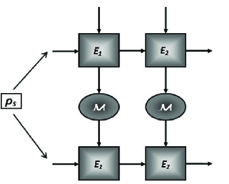
Figure 1: Communication protocol

Consider an amplitude-damping channel with finite memory for two consecutive uses, as shown in Fig. (1). The time flows from left to right while the horizontal arrows represent a two-qubit input state $\rho_{S}$. We assume that the Hilbert space of the environment $\mathcal{H}_{E}$, consists of two subspaces $\mathcal{H}_{E_{i}}$ and $\mathcal{H}_{M}$ [21]. The finite subspace $\mathcal{H}_{M}$ represents memory of the channel which does not decay over the time scale of consecutive channel uses. The subspace $\mathcal{H}_{E_{i}}$, where $i=1,2$, represents two possible states of the environment which determine the noise introduced by the channel given by Kraus operators in Eq. (9). The vertical arrows in Fig. (1) represent the influence of the interaction of first qubit with environment on the second qubit.

Mathematically, amplitude-damping channel with time-correlated Markov noise [24], is given by

$$\mathcal{E}\left(\rho_{S}\right)=\left(1-\mu\right)\sum_{i,j=0}^{1}A_{ij}^{u}\rho_{S}A_{ij}^{u{\dagger}}+\mu\sum_{k=0}^{1}A_{kk}^{c}\rho_{S}A_{kk}^{c{\dagger}},$$ (10)

where $0\leq\mu\leq 1$, is the memory parameter. In the above expression noise is uncorrelated with probability $\left(1-\mu\right)$ and the channel action is specified by Kraus operators

$$A_{ij}^{u}=A_{i}\otimes A_{j},$$ (11)

where $i,j=0,1$ with $A_{i}$ given by Eq. (9), while with probability $\mu$ it is correlated and specified by $A_{kk}^{c}$. The task of constructing Kraus operators $A_{kk}^{c}$ for the non-Pauli amplitude-damping channel is not trivial. In order to derive these operators the Lindbladian is solved using damping basis [16, 24]. The map

$$\Phi\left(\rho\right)=\exp\left(\mathcal{L}t\right)\rho=\sum_{i}\text{Tr}\left(L_{i}\rho\right)\exp\left(\lambda_{i}t\right)R_{i},$$ (12)

describes a wide class of Markov quantum channels, where $\lambda_{i}$ are the damping eigenvalues. For a finite $N$-dimensional Hilbert space

$$\mathcal{L}\rho=-\frac{1}{2}\sum_{i,j}^{N^{2}-1}c_{ij}\left(F_{j}^{{\dagger}}F_{i}\rho+\rho F_{j}^{{\dagger}}F_{i}-2F_{i}\rho F_{j}^{{\dagger}}\right),$$ (13)

and the system operators satisfy Tr$(F_{i})=0$ and Tr$\left(F_{i}^{{\dagger}}F_{j}\right)=\delta_{ij}$ while $c_{ij}$ form a positive matrix. The right eigenoperators $R_{i}$ satisfy the eigenvalue equation

$$\mathcal{L}R_{i}=\lambda_{i}R_{i},$$ (14)

and the duality relation

$$\text{Tr}\left(L_{i}R_{i}\right)=\delta_{ij},$$ (15)

with the left eigen operators $L_{i}$. The Lindbladian

$$\mathcal{L}\rho_{S}=-\frac{1}{2}\alpha\left(\sigma^{{\dagger}}\sigma\rho_{S}+\rho_{S}\sigma^{{\dagger}}\sigma-2\sigma\rho_{S}\sigma^{{\dagger}}\right),$$ (16)

yields the amplitude damping channel. The parameter $\alpha$ is analogous to the Einstein coefficient of spontaneous emission [16], and $\sigma^{{\dagger}}\equiv\frac{1}{2}\left(\sigma^{x}+i\sigma^{y}\right)$ and $\sigma\equiv\frac{1}{2}\left(\sigma^{x}-i\sigma^{y}\right)$ are the raising and lowering operators, respectively. In order to obtain time-correlated amplitude damping channel for two channel uses, Eq. (16) is modified to [24],

$$\mathcal{L}\rho_{S} = -\frac{\alpha}{2}\left[\left(\sigma^{{\dagger}}\otimes\sigma^{{\dagger}}\right)\left(\sigma\otimes\sigma\right)\rho_{S}+\rho_{S}\left(\sigma^{{\dagger}}\otimes\sigma^{{\dagger}}\right)\left(\sigma\otimes\sigma\right)\right.$$ (17)

$$\left.-2\left(\sigma\otimes\sigma\right)\rho_{S}\left(\sigma^{{\dagger}}\otimes\sigma^{{\dagger}}\right)\right].$$

The resulting completely positive and trace preserving map is given by

$$\mathcal{E}\left(\rho_{S}\right)=\sum_{i,j=0}^{3}\text{Tr}\left(L_{ij}\rho_{S}\right)\exp\left(\lambda_{ij}t\right)R_{ij}=\sum_{k=0}^{1}A_{kk}^{c}\rho_{S}A_{kk}^{c},$$ (18)

where the Kraus operators for correlated noise are

$$A_{00}^{c}=\left(\begin{array}[]{cccc}\cos\chi&0&0&0\\ 0&1&0&0\\ 0&0&1&0\\ 0&0&0&1\end{array}\right),A_{11}^{c}=\left(\begin{array}[]{cccc}0&0&0&0\\ 0&0&0&0\\ 0&0&0&0\\ \sin\chi&0&0&0\end{array}\right),$$ (19)

with $\cos\chi\equiv\exp\left(-\frac{1}{2}\alpha t\right)$ and $\sin\chi\equiv\sqrt{1-\exp\left(-\alpha t\right)}$. The Eqs. (10), (11) and (19) give the amplitude damping channel with memory. In the presence of memory, amplitude damping channel is not degradable, therefore, the maximization over the input states $N\rightarrow\infty$, can not be avoided.

3.2 Forgetful channels

If the memory of a channel decays exponentially with time and it’s output depends weakly on the initialization of memory, it is known as a forgetful channel [29]. In order to obtain a forgetful channel, double blocking strategy is used. Consider $N+L$ blocks of channel uses. The actual coding and decoding is done for the first $N$ uses, ignoring the remaining $L$ idle uses. The resulting CPT map $\overline{\mathcal{E}}_{N+L}$ acts on the states $\rho_{S}\in\mathcal{H}_{S}^{\otimes N}$. If we consider $M$ uses of such blocks, the corresponding memory channel $\overline{\mathcal{E}}_{M\left(N+L\right)}$ can be approximated by the memoryless channel $\left(\overline{\mathcal{E}}_{\left(N+L\right)}\right)^{\otimes M}$. The correlations among different blocks decay during the $L$ idle uses, which is expressed as

$$\left\|\overline{\mathcal{E}}_{M\left(N+L\right)}\left(\rho\right)-\left(\overline{\mathcal{E}}_{\left(N+L\right)}\right)^{\otimes M}\left(\rho\right)\right\|_{1}\leq h\left(m-1\right)c^{-L}$$ (20)

where $\rho\in\mathcal{H}^{\otimes MN}$ is an input state, $h$ is a constant depending on the memory model, $c>1$ ($c$ and $h$ are independent to the input state) and $\left\|.\right\|_{1}$ is the trace norm. The error committed by replacing the memory channel $\overline{\mathcal{E}}_{M\left(N+L\right)}$ with the corresponding memoryless channel $\left(\overline{\mathcal{E}}_{\left(N+L\right)}\right)^{\otimes M}$, grows with the number of blocks $M$, but it goes to zero exponentially fast with the number $L$ of idle uses in a block. This maps a quantum memory channel into memoryless one, with negligible error and permits the proof of coding theorems for this class of channels [29]. Quantum capacity $Q$ for forgetful channels is given by

$$Q=\lim_{N\rightarrow\infty}\frac{Q^{N}}{N},Q^{N}=\max_{\rho_{S}\in\mathcal{H}_{S}^{\otimes N}}I_{c}\left(\rho_{S},\mathcal{E}^{N}\right),$$ (21)

$$I_{c}=S\left[\mathcal{E}^{N}\left(\rho_{S}\right)\right]-S_{e}^{N}\left(\rho_{S}\right).$$ (22)

One might think that the capacity of $\mathcal{E}_{N+L}$ is greater than that of $\overline{\mathcal{E}}_{\left(N+L\right)}$ as the information related to the idle uses $L$ is thrown away. However, the memory channel $\overline{\mathcal{E}}_{\left(N+L\right)}$ can faithfully transmit the same amount of quantum information as the corresponding memoryless channel $\mathcal{E}_{N+L}$, with capacity given by Eq. (4). There exists a simple proof (See Appendix A in Ref. [31]) that

$$I_{c}\left(\rho^{\left(N+L\right)},\mathcal{E}_{N+L}\right)\leq I_{c}\left(\rho^{\left(N+L\right)},\overline{\mathcal{E}}_{N+L}\right)+L\log_{2}\dim\left(\mathcal{H}_{S}\right),$$ (23)

therefore, quantum capacity of these two channels coincides for $\lim_{N\rightarrow\infty}\left(L/N\right)=0$.

4 Quantum capacity of an amplitude-damping channel with memory

We now calculate the quantum capacity $Q$ for the amplitude damping channel with memory described above. Once again consider the communication system shown in Fig. (1). The information is encoded on an input state $\rho_{S}^{(2)}$ which is a generic two-qubit state given by

$$\rho_{S}^{(2)}=\rho_{S_{1}}\otimes\rho_{S_{2}},$$ (24)

with

$$\rho_{S_{i}}=\left(1-p\right)\left|0\right\rangle\left\langle 0\right|+r\left|0\right\rangle\left\langle 1\right|+r^{\ast}\left|1\right\rangle\left\langle 0\right|+p\left|1\right\rangle\left\langle 1\right|,$$ (25)

where $p$ is real and $\left|r\right|\leq\sqrt{p\left(1-p\right)}$. The input $\rho_{S}$ is part of a larger system $SR$ which is in a pure state $\left|\Psi\right\rangle$. The reference system $R$ does not evolve and is a mathematical device to purify the $\rho_{S}$. The system $\rho_{S}=$Tr${}_{R}\left(\left|\Psi\right\rangle\left\langle\Psi\right|\right)$ couples with an environment $\rho_{E}$ undergoes a unitary interaction. We know if a composite system $SR$, composed of two subsystems $S$ and $R$, is in a pure state then $S\left(\rho_{S}\right)=S\left(\rho_{R}\right)$ [36]. In this case, neither of the subsystems have any coherence. One might argue, what if the input $\rho_{S}$ is pure? The interaction between the system $\rho_{S}$ and environment $\rho_{E}$ is unitary, therefore, the coherence lost by the system is gained by the environment. If the input $\rho_{S}$ is pure, then entropy of output state $\mathcal{E}\left(\rho_{S}\right)$ and entropy exchange $S_{e}\left(\rho_{S}\right)$ are equal. In this situation, the coherent information $I_{c}$ and hence the quantum capacity $Q$ is zero. Therefore,coherent information $I_{c}$ of an amplitude-damping channel is maximized for an input with $r=0$ (for mathematical details see Appendix A), therefore we set

$$\rho_{S}^{(2)}=\left(1-p\right)^{2}\left|00\right\rangle\left\langle 00\right|+p\left(1-p\right)\left(\left|00\right\rangle\left\langle 11\right|+\left|11\right\rangle\left\langle 00\right|\right)+p^{2}\left|11\right\rangle\left\langle 11\right|.$$ (26)

This state is transmitted over the channel which maps it onto an output state

$$\mathcal{E}\left(\rho_{S}^{(2)}\right)=\left(1-\mu\right)\sum_{i,j=0}^{1}A_{ij}^{u}\rho_{S}^{(2)}A_{ij}^{u{\dagger}}+\mu\sum_{k=0}^{1}A_{kk}^{c}\rho_{S}^{(2)}A_{kk}^{c{\dagger}},$$ (27)

with eigenvalues

$$\lambda_{1} = p^{2}\cos^{2}\chi\left(\cos^{2}\chi+\mu\sin^{2}\chi\right),$$

$$\lambda_{2} = \lambda_{3}=p\cos^{2}\chi\left(1-p\cos^{2}\chi\right)+\mu p\sin^{2}\chi\left[1-p\left(1+\cos^{2}\chi\right)\right],$$

$$\lambda_{4} = \left(1-p\cos^{2}\chi\right)^{2}+\mu p\sin^{2}\chi\left[p\cos^{2}\chi-2\left(1-p\right)\right].$$ (28)

We assume without loss of generality that initially the state of the environment is pure,

$$\rho_{E}=\left(\left|00\right\rangle\left\langle 00\right|\right)_{E},$$ (29)

which after interaction with the input state $\rho_{S}^{(2)}$ is modified to

$$\rho_{E}^{\prime} = \left(1-\mu\right)\sum_{i,j,k,l=0}^{1}\text{Tr}_{S}\left(A_{ij}^{u}\rho_{S}^{(2)}A_{kl}^{u{\dagger}}\right)\left|e_{ij}\right\rangle\left\langle e_{kl}\right|$$ (30)

$$+\mu\sum_{m,n=0}^{1}\text{Tr}_{S}\left(A_{mm}^{c}\rho_{S}^{(2)}A_{nn}^{c{\dagger}}\right)\left|e_{mm}\right\rangle\left\langle e_{nn}\right|,$$

where $\left|e_{ij}\right\rangle=\left|e_{i}\right\rangle\otimes\left|e_{j}\right\rangle$ are the orthonormal basis of the environment. The eigenvalues of the output state $\rho_{E}^{\prime}$ are

$$\widetilde{\lambda}_{1} = p^{2}\sin^{2}\chi\left(\sin^{2}\chi+\mu\cos^{2}\chi\right),$$

$$\widetilde{\lambda}_{2} = \widetilde{\lambda}_{3}=\left(1-\mu\right)p\sin^{2}\chi\left(1-p\sin^{2}\chi\right),$$

$$\widetilde{\lambda}_{4} = \left(1-p\sin^{2}\chi\right)^{2}+\mu p\sin^{2}\chi\left[2-p\left(1+\sin^{2}\chi\right)\right].$$ (31)

The quantum capacity of the amplitude damping channel with Markov correlated noise, for two channel uses is calculated using Eqs. (21) and (22) which gives

$$Q^{2}=-\max_{p}\sum_{i=1}^{4}\left(\lambda_{i}\log_{2}\lambda_{i}-\widetilde{\lambda}_{i}\log_{2}\widetilde{\lambda}_{i}\right).$$ (32)

The maximization over the input probability $p$ is performed numerically. If the channel is noiseless i.e., $\chi=0\$then the capacity $Q^{2}$ is maximized for a maximally mixed input state with $p=\frac{1}{2}$. However, our results show that for $\chi\neq 0$ it is not the optimal choice for the input state. This is consistent with the earlier work for quantum capacity with correlated noise [30, 31].

Figure 2: Quantum capacity $\frac{Q^{2}}{2}$ as a function of the memory parameter $\mu$ for $\chi=\frac{\pi}{8}$, $p=0.465$ (dashed), $\chi=\frac{\pi}{6}$, $p=0.447$ (dotted), $\chi=\frac{\pi}{4}$, $p=0.389$ (dotted-dashed) and $\chi=\frac{\pi}{3}$, $p=0.312$ (solid). The capacity is normalized with respect to the number of channel uses.

In Fig. (2) we plot the quantum capacity $\frac{Q^{2}}{2}$ of the amplitude damping channel with correlated noise (normalized with respect to the number of channel uses) versus the memory coefficient $\mu$, for different values of the damping parameter $\chi$. Our results show that when the channel noise increases, the input state maximizing Eq. (32) becomes less than maximally mixed. It is evident from the plots that as the channel changes from memoryless $\mu=0$ to a perfect memory channel $\mu=1$, the quantum capacity increases, for all values of $\chi$. In particular note that for $\chi=\frac{\pi}{4}$, the capacity is zero but if the channel has non-zero memory it can transmit quantum information. Similarly, for $\chi=\frac{\pi}{3}$ the quantum capacity of the amplitude damping channel is zero unless the memory coefficient $\mu\gtrsim\frac{1}{2}$, beyond this value of $\mu$ the increase in $Q^{2}$ is almost linear. We infer that memory of an amplitude damping channel increases it’s capacity to transmit quantum information significantly.

4.1 Example: Damped harmonic oscillator

An interesting example of amplitude-damping channel with memory is given by a damped harmonic oscillator [31]. In this model, a stream of $N$ qubits (the system $Q$) interacts with the local environment of a harmonic oscillator $O$ coupled with a reservoir. The Hamiltonian of the total system is

$$\mathcal{H}\left(t\right)=\mathcal{H}_{0}+\mathcal{H}_{QO}+\delta\mathcal{H},$$ (33)

with

$$\mathcal{H}_{0}=\mathcal{H}_{Q}+\mathcal{H}_{O}=-\frac{\omega}{2}\sum_{k=1}^{N}\sigma_{k}^{z}+\upsilon\left(a^{{\dagger}}a+\frac{1}{2}\right),$$ (34)

and

$$\mathcal{H}_{QO}=\lambda\sum_{k=1}^{N}f_{k}\left(t\right)\left(a^{{\dagger}}\sigma_{k}+a\sigma_{k}^{{\dagger}}\right).$$ (35)

Here $\sigma_{z}=\left|g\right\rangle\left\langle g\right|+\left|e\right\rangle\left\langle e\right|$, while $a$ and $a^{{\dagger}}$ are the creation and annihilation operators of the harmonic oscillator. The interaction $\mathcal{H}_{QO}$ between the qubit and harmonic oscillator is of Jaynes-Cummings type. The constant $\lambda$ is real and positive and $\hbar=1$. The qubit-harmonic oscillator coupling $f_{k}\left(t\right)=1$, when qubit $k$ is inside the channel while $f_{k}\left(t\right)=0$ otherwise. Two consecutive qubits entering the channel are separated by a time interval $\tau$, and the qubit transit time is $\tau_{p}$. The term $\delta\mathcal{H}$ describes the reservoir Hamiltonian and the local environment-reservoir interaction which damps the oscillator within dissipation time scale $\tau_{d}$.

The oscillator damping is described by

$$\frac{d}{dt}\rho_{O}=\Gamma\left(a\rho_{O}a^{{\dagger}}-\frac{1}{2}a^{{\dagger}}a\rho_{O}-\frac{1}{2}\rho_{O}a^{{\dagger}}a\right),$$ (36)

which asymptotically decays to the ground state $\left|0\right\rangle$ with rate $\Gamma$ and $\tau_{d}=\frac{1}{\Gamma}$. In this case, the memory parameter can be defined as

$$\mu\equiv\frac{\tau_{d}}{\tau+\tau_{d}}.$$ (37)

The memoryless limit $\mu\ll 1$ is achieved for fast decay $\tau_{d}\ll\tau$ whereas for $\tau_{d}\approx\tau$, the memory parameter $\mu\lesssim 1$ and memory effects come into play. Arrigo et. al., solved this system numerically for two channel uses [31].

Figure 3: Capacity $\frac{Q^{2}}{2}$ as a function of the time inteval between two consecutive channel uses $\tau$ with $\chi=0.225$, $p=0.486$ (top) and $\chi=0.464$, $p=0.456$ (bottom) for $\tau_{d}=20$ (dashed) and $\tau_{d}=2$ (solid). See text for additional details.

In Fig. (3), we plot $\frac{Q^{2}}{2}$ versus $\tau$ for the same values of channel parameters as in Ref. [31]. In Eq. (32) we redefine $\mu$ as given by Eq. (37) and consider both weak $\tau_{d}=20$ and strong $\tau_{d}=2$ dissipation strength $\Gamma=\frac{1}{\tau_{d}}$ of the oscillator. The memoryless limit is recovered for $\tau\rightarrow\infty$ (for which the memory parameter $\mu\equiv\tau_{d}/\left(\tau+\tau_{d}\right)\rightarrow 0$). When the channel is less noisy with the damping parameter $\chi=0.225$, $\frac{Q^{2}}{2}$ is maximized for an input state with $p=0.486$. In this case, when $\tau_{d}$ is large, the oscillator damps to it’s ground state slowly and the channel retains it’s memory for a longer period of time. Therefore, the amount of quantum information transmitted over the channel is higher which decays to it’s minimum value at a relatively slower rate as we increase the time interval $\tau$ between two successive qubits entering the channel. In comparison, when $\tau_{d}$ is small the decay rate of the oscillator $\Gamma$ is large and it’s state decays before the second qubit enters the channel. The resulting channel is memoryless. It is evident from the plot that the quantum capacity rapidly decreases to it’s minimum value in this case. We also plot $\frac{Q^{2}}{2}$ for a lower quality channel with $\chi=0.464$ and an input state with $p=0.456$. As the channel is more noisy than the previous case therefore, less amount of quantum information is transmitted. However, once again we witness larger capacity and relatively gradual decay to it’s minimum for $\tau_{d}=20$, while smaller capacity and rapid decay for $\tau_{d}=2$. These results are consistent with the findings of Ref. [31].

5 Quantum capacity of an amplitude-damping channel with perfect memory

Finally, we consider a special case of sending an arbitrary number of qubits $N$ through an amplitude damping channel with perfect memory. It is assumed that the state of the environment remains intact for the $N$ uses. This gives an upper bound on the quantum capacity with correlated noise. Once again the double block strategy is used to make sure that the channel action over different blocks is not correlated.

The state input to the channel is an $N$ qubit state

$$\rho_{S}^{N}=\rho_{S_{1}}\otimes\ldots\otimes\rho_{S_{N}},$$ (38)

with $\rho_{S_{i}}=\left(1-p\right)\left|0\right\rangle\left\langle 0\right|+p\left|1\right\rangle\left\langle 1\right|$. This state is transmitted over an amplitude damping channel over $N$ uses of the channel. If the noise over all successive uses of the channel is perfectly uncorrelated then it maps the input state to

$$\mathcal{E}\left(\rho_{S}^{N}\right)=\sum_{u_{1}\ldots u_{N}}\left(A^{u_{1}}\otimes\ldots\otimes A^{u_{N}}\right)\rho_{S}^{N}\left(A^{u_{1}{\dagger}}\otimes\ldots\otimes A^{u_{N}{\dagger}}\right),$$ (39)

where $A^{u_{i}}\in\left[A_{o},A_{1}\right]$ and $A_{i}$ with $i=0,1$ are given in Eq. (9). The eigenvalues of the output state are

$$\gamma_{X}=p^{N}\left(\cos^{2}\chi\right)^{(N-X)}\left(1-p\cos^{2}\chi\right)^{X},$$ (40)

with $X=0,\ldots,N$. During the transmission, the input state is coupled with an environment initially assumed to be in a pure state

$$\rho_{E}^{N}=\left(\left|0\right\rangle\left\langle 0\right|\right)_{E}^{\otimes N}.$$ (41)

As a result of the interaction with the input state $\rho_{S}^{N}$, it modifies to an output state $\rho_{E}^{\prime N}$ with eigenvalues

$$\widetilde{\gamma}_{X}=p^{N}\left(\sin^{2}\chi\right)^{(N-X)}\left(1-p\sin^{2}\chi\right)^{X},$$ (42)

where $X=0,\ldots,N$. The quantum capacity can be calculated using Eqs. (21) and (22) which gives

$$Q^{N}=-\underset{p}{\max}\sum_{x=0}^{N}\left(\begin{array}[]{c}N\\ X\end{array}\right)\left[\gamma_{X}\log_{2}\gamma_{X}-\widetilde{\gamma}_{X}\log_{2}\widetilde{\gamma}_{X}\right],$$ (43)

here the binomial $\left(\begin{array}[]{c}N\\ X\end{array}\right)$ takes into account the number of times a particular eigenvalue is repeated.

Next we consider the case when the noise over the successive uses of the channel is perfectly correlated. In order to determine the Kraus operators we solve the $N$ dimensional Lindbladian

$$\mathcal{L}\rho_{S}^{N}=-\frac{1}{2}\alpha\left(\left(\sigma^{{\dagger}}\right)^{\otimes N}\left(\sigma\right)^{\otimes N}\rho_{S}^{N}+\rho_{S}^{N}\left(\sigma^{{\dagger}}\right)^{\otimes N}\left(\sigma\right)^{\otimes N}-2\left(\sigma\right)^{\otimes N}\rho_{S}^{N}\left(\sigma^{{\dagger}}\right)^{\otimes N}\right),$$ (44)

using the damping basis method outlined in Section 3. The resulting Kraus operator are

$$A_{0}^{c_{N}} = \left(\begin{array}[]{ccccc}\cos\chi&0&\cdots&0&0\\ 0&1&\cdots&0&0\\ \vdots&\vdots&\ddots&\vdots&\vdots\\ 0&0&\cdots&1&0\\ 0&0&\cdots&0&1\end{array}\right)_{2^{N}\times 2^{N}},$$ (50)

$$A_{1}^{c_{N}} = \left(\begin{array}[]{ccccc}0&0&\cdots&0&0\\ 0&0&\cdots&0&0\\ \vdots&\vdots&\ddots&\vdots&\vdots\\ 0&0&\cdots&0&0\\ \sin\chi&0&\cdots&0&0\end{array}\right)_{2^{N}\times 2^{N}}.$$ (56)

If the input state $\rho_{S}^{N}$ given by Eq. (38) is transmitted over the amplitude damping channel with perfect memory then it is mapped to an output state

$$\mathcal{E}\left(\rho_{S}^{N}\right)=\sum_{k=0}^{1}A_{k}^{c_{N}}\rho_{S}^{N}A_{k}^{{\dagger}c_{N}},$$ (57)

with eigenvalues

$$\lambda_{1} = p^{N}\cos^{2}\chi,$$

$$\lambda_{2} = \left(1-p\right)^{N}+p^{N}\sin^{2}\chi,$$

$$\lambda^{Y} = p^{N-Y}\left(1-p\right)^{Y},$$ (58)

where $Y=1,\ldots,N-1$. Similarly, the initial state of the environment $\rho_{E}^{N}$ is mapped to a state with two non-zero eigenvalues

$$\widetilde{\lambda}_{1} = p^{N}\sin^{2}\chi,$$

$$\widetilde{\lambda}_{2} = 1-p^{N}\sin^{2}\chi.$$ (59)

Using Eqs. (21) and (22) the quantum capacity is given by

$$Q^{N}=-\underset{p}{\max}\left[\sum_{i=1}^{2}\left(\lambda_{i}\log_{2}\lambda_{i}-\widetilde{\lambda}_{i}\log_{2}\widetilde{\lambda}_{i}\right)+\sum_{Y=1}^{N-1}\left(\begin{array}[]{c}N\\ Y\end{array}\right)\lambda^{Y}\log_{2}\lambda^{Y}\right].$$ (60)

The maximization over the input probability $p$ for the quantum capacity with memoryless and perfect memory channel given by Eqs. (43) and (60), respectively is performed numerically. Our calculations show that as the number of channel uses increases, the input state maximizing the capacity $Q^{N}$ changes from a less than maximally mixed state to maximally mixed state. We must evaluate the quantum capacity in the limit $N\rightarrow\infty$, therefore we infer that the maximally mixed state maximizes $Q^{N}$.

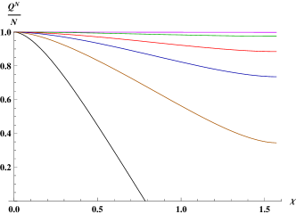
Figure 4: Capacity $\frac{Q^{N}}{N}$ versus the channel noise $\chi$ for memoryless amplitude damping channel $\mu=0$ (black) and with perfect memory $\mu=1$ for $N=2$ (brown), $N=3$ (blue), $N=4$ (red), $N=6$ (green) and $N=10$ (purple).

In Fig. (4) we plot $\frac{Q^{N}}{N}$ for both memoryless and perfect memory amplitude damping channel, versus channel noise parameter $\chi$. We set $p=\frac{1}{2}$, for all channel uses. The memoryless amplitude damping channel is degradable and it’s quantum capacity $Q$ is additive given by $Q=Q_{1}$, hence we have only one curve in the plot for this case. It shows that the quantum capacity decreases to zero as the memoryless amplitude damping channel becomes noisy. However, in the presence of perfect memory we will always have non-zero quantum capacity, even if the channel noise is maximum i.e., $\chi=\frac{\pi}{2}$. It is evident that as the number of channel uses increase, the capacity converges to it’s maximum value $Q=1$.

6 Conclusion

We have studied an amplitude-damping with memory and calculated it’s capacity to transmit quantum information. Our results show that the quantum capacity of the channel increases if the noise over the consecutive uses of the channel is correlated, independent of the damping parameter $\chi$. If the memory of the channel $\mu\gtrsim\frac{1}{2}$, we will always have non-zero quantum capacity even if the channel noise attains it’s maximum allowed value. As compared to the numerical results reported in [31] for an amplitude-damping channel with memory we determine the quantum capacity analytically. The comparison of our study with their results for the same set of channel parameter shows similar behaviour with the increase of channel memory. In the case of amplitude-damping channel with perfect memory channel, we calculate the quantum capacity, for an arbitrary number of channel uses. Our results show that the quantum capacity will always be non-zero if the channel has perfect memory and saturates to it’s maximum value in the limit $N\rightarrow\infty$.

Appendix A Dependence of coherent information on $\left|r\right|^{2}$

Consider the two-qubit input state $\rho_{S}^{(2)}$ given by Eq. (24). For mathematical simplicity, we diagonalize the input state such that

$$\rho_{S_{i}}=\frac{1}{2}\left[\left(1-\Gamma\right)\left|0\right\rangle\left\langle 0\right|+\left(1+\Gamma\right)\left|1\right\rangle\left\langle 1\right|\right],$$ (61)

where $\Gamma=\sqrt{(1-2p)^{2}+4\left|r\right|^{2}}$ and $0\leq\left|r\right|^{2}\leq p\left(1-p\right)$. This state is transmitted over an amplitude-damping channel with memory given by Eq. (10), which maps it to an output state with eigenvalues

$$\upsilon_{1} = \frac{1}{4}\left(1-\Gamma\right)^{2}\cos^{2}\chi\left(\cos^{2}\chi+\mu\sin^{2}\chi\right),$$

$$\upsilon_{2} = \upsilon_{3}=\frac{1}{2}\cos^{2}\chi\left[\left(1-\Gamma\right)\sin^{2}\chi+2\Lambda\cos^{2}\chi\right]$$

$$+\mu\left[\Lambda\left(1-\cos^{4}\chi\right)-\frac{1}{2}\left(1-\Gamma\right)\cos^{2}\chi\sin^{2}\chi\right],$$

$$\upsilon_{4} = \frac{1}{2}\left[1+\sin^{4}\chi+\Gamma\left(1-\sin^{4}\chi\right)-2\Lambda\cos^{4}\chi\right.$$ (62)

$$\left.+\mu\left(1-\Gamma\right)\cos^{2}\chi\sin^{2}\chi-2\Lambda\sin^{2}\chi\left(2+\cos^{2}\chi\right)\right],$$

with $\Lambda=p\left(1-p\right)-\left|r\right|^{2}$. We assume that the environment is initially in a pure state $\rho_{E}$ given by Eq. (29). The interaction with $\rho_{S}^{(2)}$, modifies the environment to an output state $\rho_{E}^{\prime}$ with eigenvalues

$$\widetilde{\upsilon}_{1} = \frac{1}{4}\left(1-\Gamma\right)^{2}\sin^{2}\chi\left(\sin^{2}\chi+\mu\cos^{2}\chi\right),$$

$$\widetilde{\upsilon}_{2} = \widetilde{\upsilon}_{3}=\frac{1}{4}\left(1-\mu\right)\sin^{2}\chi\left(4\Lambda+\left(1-\Gamma\right)^{2}\cos^{2}\chi\right),$$

$$\widetilde{\upsilon}_{4} = \frac{1}{4}\left[4\Gamma+\left(1-\Gamma\right)^{2}\left(1+\cos^{4}\chi\right)+8\Lambda\cos^{2}\chi+\mu\left\{4\Lambda\left(\sin^{2}\chi-2\cos^{2}\chi\right)\right.\right.$$ (63)

$$\left.\left.+2\left(1-\Gamma\right)\left(1+\cos^{2}\chi\right)-\left(1-\Gamma\right)^{2}\left(1+\cos^{4}\chi\right)\right\}\right].$$

Here, we have used Eq. (30), to determine $\rho_{E}^{\prime}$ with $\rho_{S_{i}}$ given by Eq. (61). Once we have the eigenvalues for the output states, the coherent information $I_{c}$ and quantum capacity $\frac{Q^{2}}{2}$, for two channel uses, is calculated from Eqs. (21) and (22), respectively.

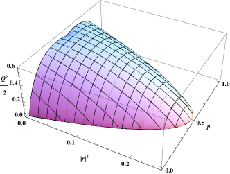
Figure 5: Capacity $\frac{Q^{2}}{2}$ versus the input probability distribution $p$ and coherence  $\left|r\right|^{2}$, for $\mu=0.8$ and channel parameter $\chi=0.685$.

In Fig. (5), we plot $\frac{Q^{2}}{2}$ versus the probability of input state $p$ and coherence $\left|r\right|^{2}$, for fixed values of channel noise $\chi$ and memory $\mu$. It shows that for all possible values of $p$, the capacity decreases as we increase coherence, acquiring it’s minimum value zero when coherence of the input state is maximum, that is, $\left|r\right|^{2}=p\left(1-p\right)$. We conclude that coherent information $I_{c}$, is maximized for an input state for which $\left|r\right|^{2}=0$. The maximization over $p$, in Eq. (21) is performed numerically. For an amplitude-damping channel with $\chi=0.685$, $\frac{Q^{2}}{2}$ is maximized for $p=0.4154$. Therefore, in Fig. (5), there is a slight decrease in $\frac{Q^{2}}{2}$, for $\left|r\right|^{2}=0$ at $p=0.5$. If $\left|r\right|^{2}=0$ then $\Gamma=1-2p$ and $\Lambda=p\left(1-p\right)$, the eigenvalues of Eq. (28) and Eq. (31) are retrieved and the results are discussed in Section 4 . However, when the coherence is maximum, then $\Gamma=1$ and $\Lambda=0$, both the system and environment are pure and quantum capacity $\frac{Q^{2}}{2}$ is zero. This is in agreement with the findings of Refs. [19, 31].

Acknowledgement 1

N. Arshed was supported by the Higher Education Commission Pakistan under Grant No. 063-111368-Ps3-001.

References

• [1] C. Shannon, Bell Sys. Tech. J. 27, 379 (1948).
• [2] T. M. Cover and J. A. Thomas, Elements of Information Theory (Wiley, New York, 1991).
• [3] C. H. Bennett and P. W. Shor, Science 303, 1784 (2004).
• [4] C. Bennett and P. W. Shor, IEEE Trans. Inf. Theory 44, 2724 (1998).
• [5] P. Hausladen, R. Jozsa, B. Schumacher, M. Westmoreland and W. K. Wootters, Phys. Rev. A 54, 1869 (1996).
• [6] B. Schumacher and M. D. Westmoreland, Phys. Rev. A 56, 131 (1997).
• [7] S. Lloyd, Phys. Rev. A 55, 1613 (1997).
• [8] P. W. Shor, The quantum channel capacity and coherent information, Tech. Rep. Lecture Notes MSRI Workshop on quantum computation (2002) [http://www.msri.org/publications/In/msri/2002/quantumcrypto/shor/1/].
• [9] I. Devetak, IEEE Trans. Inf. Theory 51, 44 (2005).
• [10] H. Barnum, M. A. Neilson and B. Schumacher, Phys. Rev. A 57, 4153 (1998).
• [11] C. H. Bennett, D. P. DiVincenzo and J. A. Smolin, Phys. Rev. Lett. 78, 3217 (1997).
• [12] C. Adami and N. J. Cerf, Phys. Rev. A 56, 3470 (1997).
• [13] C. H. Bennett, P. W. Shor, J. A. Smolin and A. V. Thapliyal, Phys. Rev. Lett. 83, 3081 (1999).
• [14] C. H. Bennett, P. W. Shor, J. A. Smolin and A. V. Thapliyal, IEEE Trans. Inf. Theory 48, 2637 (2002).
• [15] A. S. Holevo, J. Math. Phys. 43, 4326 (2002).
• [16] S. Daffer, K. Wodkiewicz, and J. K. McIver, Phys. Rev. A 67, 062312 (2003).
• [17] P. W. Shor, Quantum Inf. Comput. 4, 537 (2004).
• [18] D. Krestschmann and R. F. Werner, New J. Phys. 6, 26 (2004).
• [19] V. Giovannetti and R. Fazio, Phys. Rev. A 71, 032314 (2005).
• [20] M. M. Wolf and D. P. Garcia, Phys. Rev. A 75, 012303 (2007).
• [21] G. Bowen and S. Mancini, Phys. Rev. A 69, 012306 (2004).
• [22] C. Macchiavello and G. M. Palma, Phys. Rev. A 65, 050301(R) (2002).
• [23] C. Macchiavello, G. M. Palma, and S. Virmani, Phys. Rev. A 69, 010303(R) (2004).
• [24] Y. Yeo and A. Skeen, Phys. Rev. A 67, 064301 (2003).
• [25] N. Arshed and A. H. Toor, Phys. Rev. A 73, 014304 (2006).
• [26] A. D’ Arrigo, G. Benenti and G. Falci, New J. Phys. 9, 310 (2007).
• [27] M. B. Plenio and S. Virmani, Phys. Rev. Lett. 99, 120504 (2007).
• [28] A. Bayat, D. Burgarth, S. Mancini and S. Bose, Phys. Rev. A 77, 050306(R) (2008).
• [29] D. Kretschmann and R. F. Werner, Phys. Rev. A 72, 062323 (2005).
• [30] G. Benenti, A. D’ Arrigo and G. Falci, Phys. Rev. Lett. 103, 020502 (2009).
• [31] A. D’ Arrigo, G. Benenti and G. Falci, Eur. Phys. J. D 66, 147 (2012).
• [32] I. Bjelakovic, H. Boche and J. Noetzel, Phys. Rev. A 78, 042331 (2008).
• [33] I. Bjelakovic, H. Boche and J. Noetzel, arXiv: 0808.1007 (2008).
• [34] I. Bjelakovic, H. Boche and J. Noetzel, arXiv: 0811.4588 (2009).
• [35] I. Devetak and P. W. Shor, Commun. Math. Phys. 256, 287 (2005).
• [36] M. Neilson and I. Chuang, Quantum Computation and Quantum Information (Cambridge University Press, Cambridge, UK, 2000).
• [37] K. Kraus, States, Effects and Operations: Fundamental Notations of Quantum Theory (Springer-Verlag, Berlin, 1983).
• [38] C. King, K. Matsumoto, M. Nathanson and M. B. Ruskai, Markov Process Relat. Fields 13, 391 (2007).
• [39] B. Schumacher, Phys. Rev. A 54, 2614 (1996).
• [40] C. King and M. B. Ruskai, IEEE Trans. Inf. Theory 47, 192 (2001).