Synchronization of Josephson oscillations in mesa array of $\rm{Bi_{2}Sr_{2}CaCu_{2}O_{8+\delta}}$ single crystal through the Josephson plasma waves in base crystal

Abstract

Using mesa array of $\rm{Bi_{2}Sr_{2}CaCu_{2}O_{8}}$ single crystal was demonstrated recently as a promising route to enhance the radiation power generated by Josephson oscillations in mesas. We study the synchronization in such an array via the plasma waves in the base crystal. First, we analyze plasma oscillations inside the base crystal generated by the synchronized mesa array and the associated dissipation. We then solve the dynamic equation for superconducting phase numerically to find conditions for synchronization and to check the stability of synchronized state. We find that mesas are synchronized when the cavity resonance of mesas matches with that of the base crystal. An optimal configuration of mesa arrays is also obtained.

I Introduction

Soon after the discovery of Josephson Effects, it was realized that Josephson junction can be used to generate electromagnetic waves. When the junction is biased in voltage state with voltage $V$, the two superconducting electrodes have energy difference $2eV$. The system is similar to two-energy level system in atomic physics. When Cooper pairs tunnel from the electrode with higher energy to that with lower energy, a photon with angular frequency $\omega=2eV/\hbar$ is emitted. The frequency can be tuned by voltage and $1$ mV corresponds to $0.483$ THz. The radiation power from one junction however is weak, of the order of 1 pW. Yanson et al. (1965); Dayem and Grimes (1966); Zimmerma.Je et al. (1966) Arrays of Josephson junctions are fabricated to enhance the radiation powerFinnegan and Wahlsten (1972); Jain et al. (1984); Darula et al. (1999); Barbara et al. (1999); Song et al. (2009). Once these junctions are synchronized, the total radiation power is proportional to the number of junctions squared.

A stack of Josephson junctions is naturally realized in some layered cuprate superconductorKleiner et al. (1992), such as $\rm{Bi_{2}Sr_{2}CaCu_{2}O_{8+\delta}}$ (BSCCO). Because of the large superconducting energy gap (60 meV), these build-in intrinsic Josephson junctions (IJJs) may have Josephson oscillations with frequencies in the terahertz (THz) band. IJJs are packed on nanometer scale, much smaller than THz electromagnetic (EM) wavelength, and are homogeneous. The THz generator based on IJJs thus is promising to fill the THz gapHu and Lin (2010); Savel’ev et al. (2010). Lots of effort has been made to excite the coherent THz radiation experimentally in the last decade Iguchi et al. (2000); Batov et al. (2006); Bae et al. (2007); Benseman et al. (2011). On the theoretical side, numerical simulations and analytical calculations are performed to understand the mechanism of radiation. Tachiki et al. (1994); Koyama and Tachiki (1995); Tachiki et al. (2005); Bulaevskii and Koshelev (2006a, 2007); Lin et al. (2008); Koshelev and Bulaevskii (2008); Tachiki et al. (2009); Lin and Hu (2009)

Coherent radiations from a mesa structure of BSCCO in the absence external magnetic fields were observed experimentally in 2007Ozyuzer et al. (2007), which renewed the interest in this field. It was found that the mesa itself forms a cavity to synchronize the radiation in different layers, as evidenced from the dependence of the radiation frequency $f$ on the lateral size $L$ of the mesa, $f=c_{0}/(2L)$ with $c_{0}=c/\sqrt{\epsilon_{c}}$ the Josephson plasma velocity where $\epsilon_{c}$ is the dielectric constant of BSCCO. The cavity resonance mechanism has been confirmed by many independent experimentsKadowaki et al. (2008); Wang et al. (2009, 2010); Tsujimoto et al. (2010, 2012) and the radiation power is enhanced to about $30\ \rm{\mu W}$.Yamaki et al. (2011) A dynamic state with $\pi$ phase kink was proposed to account for the experimental observations Lin and Hu (2008); Koshelev (2008). It was suggested that the strong in-plane dissipation is responsible for the excitation of cavity mode uniform along the $c$-axis. Lin and Hu (2012)

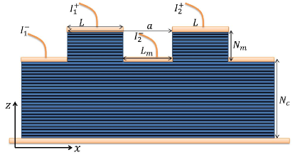
Figure 1: (color online) Schematic view of multiple mesas atop of BSCCO crystal. The mesas are biased independently. The BSCCO sample (blue) is sandwiched by gold electrodes (orange). In analytical treatment, we consider an array of identical mesas with width $L$ and period $a$. The top surface of the base crystal is free. In simulations, we consider two identical mesas with width $L$ separated by a distance $L_{m}$. The mesas are located at the position $L$ away from the edges of the base crystal. The top surface of the base crystal is also covered by gold electrodes through which the current is extracted.

From application perspective, the radiation power in the present experimental design is still too weak to be practically useful. A natural way to enhance the radiation power by using thicker mesas has several challenges. First, for a thick mesa it becomes difficult to cool the system efficiently. The dissipation hence self-heating increases with the volume of the mesa, while the heat removal rate remains the same because the heat is mainly removed through the substrate. It has already shown experimentally that even for a mesa with thickness of $\sim 2\rm{\mu m}$, central part of the meas is driven to the normal state by the severe self-heating.Wang et al. (2009, 2010). Secondly, it was calculated that for a tall mesa a long-range instability destroying the in-phase plasma oscillations developsKoshelev (2010), and only parts of the mesa can be synchronized.Lin and Hu (2012)

To enhance the radiation power while minimizing the self-heating, one may use multiple thin mesas on top of the same BSCCO single crystal. The multiple mesa structure has been fabricated recently and the radiation power is enhanced under appropriate conditions as demonstrated in the recent experiments.Orita et al. (2010); Benseman et. al. (2012) The mechanism of synchronization among mesas is not known. There are two sources of interaction. The mesas interact through the radiation fields. They also interact through the plasma oscillations in the base crystal. The resonance damping due to the leaking of radiation from the mesa into the base crystal has been considered in Ref. Koshelev and Bulaevskii, 2009 and it was demonstrated that this channel gives the main contribution to the dissipation. Therefore, synchronization mediated by radiation fields inside crystal is probably a dominating mechanism. The present work is devoted to understanding the synchronization of multiple mesas through plasma oscillations in the base crystal and to finding an optimal configuration for synchronization.

II Model

We consider arrays of identical mesas with the period $a$ atop of BSCCO single crystal as schematically shown in Fig. 1. Every mesa contains $N_{\mathrm{m}}$ junctions and has width $L$ while the base crystal contains $N_{c}$ junctions. No external magnetic field is applied to the BSCCO. Each mesa is biased independent by a dc current injected from top of the mesa and extracted from the sides of the mesa. In this case, the junctions in the basal crystal remain zero-voltage state, and the mesas are driven into resistive state. The system is assumed to be uniform along the $y$ direction and the problem becomes two dimensional. The dynamics of the gauge invariant phase difference $\theta_{n}$ and magnetic field $h_{n}$ in the $n$-th junction are described by Sakai et al. (1993); Bulaevskii et al. (1994, 1996); Machida et al. (1999); Koshelev and Aranson (2001)

$$\frac{\partial^{2}\theta_{n}}{\partial\tau^{2}}+\nu_{c}\frac{\partial\theta_{n}}{\partial\tau}+\sin\theta_{n}-\ell^{2}\frac{\partial h_{n}}{\partial x}=0,$$ (1)

$$\left(\ell^{2}\nabla_{n}^{2}-1\right)h_{n}+\frac{\partial\theta_{n}}{\partial x}+\nu_{ab}\frac{\partial}{\partial\tau}\left(\frac{\partial\theta_{n}}{\partial x}-h_{n}\right)=0,$$ (2)

where $\Delta^{(2)}f_{l}\equiv f_{l+1}+f_{l-1}-2f_{l}$ is the finite difference operator. Here the time and coordinate are measured in units of the inverse Josephson plasma frequency $1/\omega_{p}$ and the Josephson length $\lambda_{J}=\gamma s$ correspondingly and the unit of magnetic field is $\Phi_{0}/(2\pi\gamma s^{2})$, where $\gamma$ is the anisotropy factor and $s$ is the interlayer spacing. Here $\omega_{p}=c/(\lambda_{c}\sqrt{\epsilon_{c}})$ and $\Phi_{0}=hc/(2e)$ is the flux quantum. These reduced equations depend on three parameters, $\nu_{c}\!=\!4\pi\sigma_{c}/(\varepsilon_{c}\omega_{p})$, $\nu_{ab}\!=\!4\pi\sigma_{ab}/(\varepsilon_{c}\omega_{p}\gamma^{2})$, and $\ell\!=\!\lambda_{ab}/s$, where $\sigma_{c}$ and $\sigma_{ab}$ are the quasiparticle conductivity, and $\lambda_{c}$ and $\lambda_{ab}$ are the London penetration depth along the $c$-axis and $ab$-plane respectively. The dimensionless electric field is given by $E_{z,n}=\partial_{t}\theta_{n}$, with $E$ in unit of $\Phi_{0}\omega_{p}/(2\pi cs)$.

For the mesa with thickness of $1\ \rm{\mu m}$ which is much smaller than the wave length of THz EM wave in vacuum, there is a significant impedance mismatch between the mesa and vacuumBulaevskii and Koshelev (2006b). Most part of energy is reflected at the edges of mesa and cavity resonance is achieved. We can use the boundary condition that the oscillating magnetic field vanishes at the edges. The boundary condition at the edges of the mesas is $\partial_{x}\theta_{n}=\pm LI_{\mu}/2$, and the boundary condition at the edges of the base crystal is $\partial_{x}\theta_{n}=0$, where $I_{\mu}$ is the bias current in the $\mu$-th mesa. We assume that the IJJs stack is sandwiched by good conductors, such that the tangential current inside the conductor is zero, which corresponds to the boundary condition $\partial_{z}h(z)=0$ in the continuum limit.

III Plasma oscillations and associated dissipation in the synchronized state

In this section, we calculate the plasma oscillations and its dissipation in the synchronized state assuming that the array contains large number of mesas so that it can be treated as an infinite system. The time dependence of the phases in mesas in resistive state has the form $\theta_{n}(x,t)=\omega\tau+\varphi_{n}(x)+\operatorname{Re}[\theta_{n}(x)\exp(-i\omega\tau)]+\psi_{\mu}$ and in the crystal the phases have only have small oscillations. Here $\psi_{\mu}$ accounts for the phase shift between synchronized mesas. We consider the case with $\psi_{\mu}=0$ and leave the more general case for numerical simulation in the next Section. We consider voltage range corresponding to the Josephson frequency close to fundamental cavity resonance $\omega\approx\omega_{1}=\ell\pi/L$. For definiteness, we assume that in mesas the kink state is formed Lin and Hu (2008); Koshelev (2008) providing strong coupling to the cavity resonance meaning that we can use approximations $\varphi_{n}(x)\approx\pi\mathrm{sgn}(x)$ and $\sin\theta_{n}=\operatorname{Re}[i\exp(-i\omega\tau-i\varphi_{n}(x))]\approx g(x)\operatorname{Re}[i\exp(-i\omega\tau)]$ with $g(x)\approx\mathrm{sgn}(x)$. However, a particular shape of the modulation function $g(x)$ has no importance in further derivations. For isolated mesa on the top of bulk crystal this problem was considered in Ref. Koshelev and Bulaevskii, 2009 where it was concluded that leaking radiation into crystal provides dominating mechanism of resonance damping.

The amplitudes of phases and magnetic fields obey the following equations: in mesas for $|x-ma|<L/2$, $0<n<N_{\mathrm{m}},$

$$\left(\omega^{2}+i\nu_{c}\omega\right)\theta_{n}+\ell^{2}\frac{\partial h_{n}}{\partial x} =ig(x),$$ (3)

$$\ell^{2}\nabla_{n}^{2}h_{n}-\left(1-i\nu_{ab}\omega\right)h_{n}+\left(1-i\nu_{ab}\omega\right)\frac{\partial\theta_{n}}{\partial x} =0,$$ (4)

and in the crystal, for $-N_{c}<n\leq 0$, the first equation has to be modified as

$$\left(\omega^{2}-1+i\nu_{c}\omega\right)\theta_{n}+\ell^{2}\frac{\partial h_{n}}{\partial x}=0.$$ (5)

Using presentation $g(x)=\sum_{m=0}^{\infty}g_{m}\sin\left(p_{m}x\right)$ with $p_{m}=(2m-1)\pi/L$, we can find solution of these equations as mode expansions. In particular, the oscillating magnetic field in mesas can be written as

$$h_{n}^{(\mathrm{m})}(x)=\sum_{m=1}^{\infty}\frac{ip_{m}(g_{m}\!+\!a_{m}\cos\left[q_{m}\left(n\!-\!N_{\mathrm{m}}\!-\!1/2\right)\right])}{\omega^{2}+i\nu_{c}\omega-\ell^{2}p_{m}^{2}}\cos\left(p_{m}x\right)$$ (6)

for $n>0$, where $q_{m}\equiv q(p_{m},\omega)$ with $\mathrm{Im}(q_{m})>0$ is the wave vector describing propagation of the plasma wave along $c$-axis for the fixed in-plane wave vector and frequency,

$$\cos q_{m}=1+\frac{1-i\nu_{ab}\omega}{2\ell^{2}}\left(1-\frac{\ell^{2}p_{m}^{2}}{\omega^{2}+i\nu_{c}\omega}\right)$$ (7)

In crystal, $n\leq 0$, the oscillating magnetic field can be presented as Fourier series,

$$h_{n}^{(\mathrm{cr})}(x) =\frac{1}{a}\sum_{k=2\pi l/a}H_{k}\cos\left[q_{k}\left(n+N_{c}+1/2\right)\right]\exp(ikx)$$ (8)

with $$\cos q_{k}=1+\frac{1-i\nu_{ab}\omega}{2\ell^{2}}\left(1-\frac{\ell^{2}k^{2}}{\omega^{2}-1+i\nu_{c}\omega}\right).$$

It is crucial that the synchronized mesa array excites discrete set of modes inside the crystal. For the fixed $k$ the frequency range $\omega^{2}<1+\ell^{2}k^{2}$ corresponds to propagating waves along the $c$-axis while the range $\omega^{2}>1+\ell^{2}k^{2}$ corresponds to evanescent waves. At the frequency $\omega^{2}=1+\ell^{2}k^{2}$ the uniform plasma mode is excited. The decay length of the plasma mode in terms of the number of junctions, $N_{d}(\omega)=1/\mathrm{Im}(q_{k}(\omega))$, has a sharp maximum at this frequency, see Fig. 2. For $a\approx 2L$ the mode with the wave vector $k=2\pi/a$ plays the most important role, because frequency of the uniform mode $\omega=\sqrt{1+\ell^{2}(2\pi/a)^{2}}$ is close to the cavity-resonance frequency inside the mesa $\omega_{1}=\ell\pi/L$.

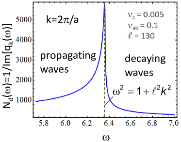
Figure 2: (color online) The frequency dependence of the decay length along $c$-direction, $N_{d}$, for the fixed in-plane wave vector and representative parameters specified in the plot.

The unknown coefficients $a_{m}$ and $H_{k}$ have to be found from matching at the interface, $h_{n}^{(\mathrm{m})}(x)=h_{n}^{(\mathrm{cr})}(x)$ for $n=0,1$. Taking the projection of the equation $h_{0}^{(\mathrm{m})}(x)=h_{0}^{(\mathrm{cr})}(x)$ to mode $m$, using

$$S_{m}(k)=\int_{-L/2}^{L/2}dx\cos\left(p_{m}x\right)\cos kx=\frac{2(-1)^{m}p_{m}\cos\left[kL/2\right]}{p_{m}^{2}-k^{2}},$$ (9)

we obtain equation expressing $a_{m}$ via $H_{k}$

$$\frac{ip_{m}\left(g_{m}+a_{m}\cos\left[q_{m}\left(N_{\mathrm{m}}\!+\!1/2\right)\right]\right)}{\omega^{2}+i\nu_{c}\omega-\ell^{2}p_{m}^{2}}$$

$$=\frac{1}{a}\sum_{k=2\pi l/a}H_{k}\cos\left[q_{k}\left(N_{c}+1/2\right)\right]\frac{4(-1)^{m}}{L}\frac{p_{m}\cos\left[kL/2\right]}{p_{m}^{2}-k^{2}}.$$

Note that $S_{m}(k)$ satisfy orthogonality conditions

$$\frac{2}{aL}\sum_{k=2\pi l/a}S_{m}(k)S_{m^{\prime}}(k)=\delta_{mm^{\prime}}.$$

On the other hand, the inverse Fourier transform of the equation $h_{1}^{(\mathrm{m})}(x)=h_{1}^{(\mathrm{cr})}(x)$ allows us to express $H_{k}$ via $a_{m}$

$$H_{k}\cos\left[q_{k}\left(N_{c}+3/2\right)\right] =\sum_{m=1}^{\infty}\frac{ip_{m}\left(g_{m}+a_{m}\cos\left[q_{m^{\prime}}\left(N_{\mathrm{m}}-1/2\right)\right]\right)}{\omega^{2}+i\nu_{c}\omega-\ell^{2}p_{m}^{2}}$$

$$\times\frac{2(-1)^{m}p_{m}\cos\left[kL/2\right]}{p_{m}^{2}-k^{2}}$$ (10)

Eliminating $H_{k}$, we obtain the linear equations for $a_{m}$

$$\left(\cos\left[q_{m}\left(N_{\mathrm{m}}-1/2\right)\right]-\cos\left[q_{m}\left(N_{\mathrm{m}}+1/2\right)\right]\right)a_{m}$$

$$-\sum_{m^{\prime}=1}^{\infty}\mathcal{J}_{mm^{\prime}}a_{m^{\prime}}\cos\left[q_{m^{\prime}}\left(N_{\mathrm{m}}-1/2\right)\right]=\sum_{m^{\prime}=1}^{\infty}\mathcal{J}_{mm^{\prime}}g_{m^{\prime}}$$ (11)

with the matrix

$$\mathcal{J}_{mm^{\prime}} =\frac{p_{m^{\prime}}\left(\omega^{2}+i\nu_{c}\omega-\ell^{2}p_{m}^{2}\right)}{p_{m}\left(\omega^{2}+i\nu_{c}\omega-\ell^{2}p_{m^{\prime}}^{2}\right)}\frac{2}{aL}$$

$$\times\sum_{k=2\pi l/a}S_{m}(k)S_{m^{\prime}}(k)\left(1-\frac{\cos\left[q_{k}\left(N_{c}+1/2\right)\right]}{\cos\left[q_{k}\left(N_{c}+3/2\right)\right]}\right).$$

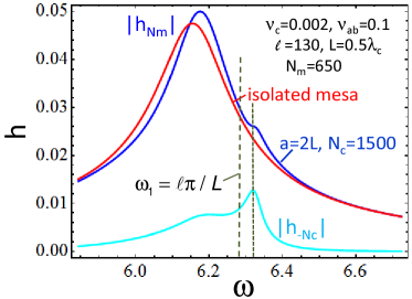
Figure 3: (color online) Comparison of the frequency dependence of the oscillating magnetic field at the mesa top for isolated mesa and mesa array. The frequency dependence of the oscillating magnetic field at the bottom of the base crystal for mesa array is also shown. Parameters used in calculations are specified in the plot.

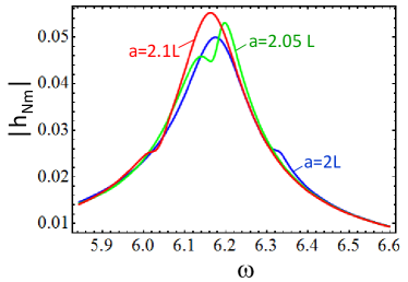
Figure 4: (color online) The frequency dependences of the oscillating magnetic field at the mesa top for different periods of the mesa array. Other parameters are the same as in the previous plot.

Near the fundamental-mode resonance $\omega\approx\ell p_{1}$ the amplitude $a_{1}$ dominates and we can use single-mode approximation neglecting all other amplitudes. This leads to a simple result

$$a_{1} \approx\frac{g_{1}\mathcal{J}_{11}}{\cos\left[q_{1}\left(N_{\mathrm{m}}-1/2\right)\right]-\left(1+\mathcal{J}_{11}\right)\cos\left[q_{1}\left(N_{\mathrm{m}}+1/2\right)\right]}$$

$$\approx\frac{g_{1}\mathcal{J}_{11}}{q_{1}\sin\left[q_{1}N_{\mathrm{m}}\right]-\mathcal{J}_{11}\cos\left[q_{1}\left(N_{\mathrm{m}}+1/2\right)\right]}$$ (12)

with

$$\mathcal{J}_{11}=\frac{2}{aL}\sum_{k=2\pi l/a}\frac{4p_{1}^{2}\cos^{2}\left[kL/2\right]}{(p_{1}^{2}-k^{2})^{2}}\left(1-\frac{\cos\left[q_{k}\left(N_{c}+1/2\right)\right]}{\cos\left[q_{k}\left(N_{c}+3/2\right)\right]}\right)$$ (13)

and $q_{1}\approx\sqrt{-\frac{1-i\nu_{ab}\omega}{\ell^{2}}\frac{\omega^{2}-\ell^{2}p_{1}^{2}+i\nu_{c}\omega}{\omega^{2}+i\nu_{c}\omega}}$. With this result, one can obtain the oscillating phases and fields in the mesa. Also using Eq. (10) and keeping only $m=1$ in the sum, we obtain the coefficients $H_{k}$ which determine the oscillating magnetic field inside the crystal, Eq. (8). For an isolated mesa on bulk crystal corresponding to the limit $a,N_{c}\rightarrow+\infty$, the following approximate result can be derivedKoshelev and Bulaevskii (2009) $\mathcal{J}_{11}\approx{\sqrt{1-i\nu_{ab}\omega}}\left(0.57+0.31i\right)/{\ell}$, suggesting the following presentation $\mathcal{J}_{11}={\sqrt{1-i\nu_{ab}\omega}}\beta_{1}/{\ell}$, where $\beta_{1}$ is the complex function of the order unity. The amplitude of the oscillating magnetic field on the top of the mesa can be represented as

$$h_{N_{\mathrm{m}}}^{(\mathrm{m})}(x)\approx\frac{ip_{1}g_{1}\cos\left(p_{1}x\right)}{\omega^{2}-\ell^{2}p_{1}^{2}+i\nu_{c}\omega+\mathcal{A}_{1}(\omega)},$$ (14)

where the complex function $\mathcal{A}_{1}(\omega)$

$$\mathcal{A}_{1}\!=\!-\frac{\left(\omega^{2}-\ell^{2}p_{1}^{2}+i\nu_{c}\omega\right)\beta_{1}}{\sqrt{-\frac{\omega^{2}-\ell^{2}p_{1}^{2}+i\nu_{c}\omega}{\omega^{2}+i\nu_{c}\omega}}\sin\left[q_{1}N_{\mathrm{m}}\right]\!+\!\beta_{1}\!\left(1\!-\!\cos\left[q_{1}\!\left(N_{\mathrm{m}}\!-\!\frac{1}{2}\right)\right]\right)}.$$

determines the damping of the resonance and its frequency shift in all quantities.

Figure 3 illustrates the Josephson-frequency dependence of the oscillating magnetic field amplitude inside the mesa near the cavity-resonance frequency for isolated mesa and for mesa array with $a=2L$. One can see that for used parameters the corrections are weak. Above the main peak one can see a small dip caused to excitation of the almost uniform standing wave inside the crystal. To verify this, we also show the plot of the oscillating magnetic field at the bottom of the base crystal. The dip in the mesa field corresponds to the rather sharp peak of the field at the bottom of the crystal. Note also that the resonance is displaced to lower frequency with respect to the uniform cavity mode $\ell\pi/L$ because plasma oscillations excited inside the mesa are not uniform in the c direction. The width of resonance is mostly determined my leak of radiation into the base crystal.

Figure 4 shows evolution of the resonance shape with variation of the array period $a$. We can see that with increasing $a$ the dip moves to smaller frequencies. The dip has maximum amplitude and located at the peak for $a=2.05L$. It is interesting to note that the resonance in mesa is actually strongest when the dip is located below the peak at $a=2.1L$. The reason is that in this case the wave excited at the peak frequency and the wave vector $k=2\pi/a$ is in decaying range, see Fig. 2 and, as consequence, the mesas loose less energy to radiation at the resonance frequency. Nevertheless, we expect the strongest interaction between the mesas and optimal conditions for synchronization when resonances coincide.

Figure 5: (color online) Phase coherence of plasma oscillations between different stacks for different $L_{m}$. The phase coherence is measured by $|g_{j,L/R}|$ defined in Eq. (16).

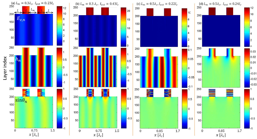
Figure 6: (color online) Snapshots of the electric field (first row), magnetic field (second row) and Josephson current $\sin(\theta_{n})$ (third row) in the whole system. (a) and (b) are obtained at the first and second cavity resonance for $L_{m}=L$. (c) and (d) are results near the first cavity resonance for $L_{m}\neq nL$.

IV Numerical Simulations

To find the condition for synchronization between mesas and checked the stability of the synchronized state, we solve Eqs. (1) and (2) numerically for two mesas and numerical details are presented in Ref. Lin and Hu, 2012. The number of junctions in the base is $N_{c}=200$ and in the mesa is $N_{m}=50$. We take $\nu_{c}=0.02$, $\nu_{ab}=0.2$ and $\ell\!=\!266.5$. To ensure that the resulting state is stable, we add an artificial weak white noise current in Eq. (1) in simulations, $\left\langle\tilde{I}_{n}(x,t)\tilde{I}_{n^{\prime}}(x^{\prime},t^{\prime})\right\rangle=10^{-5}\delta(x-x^{\prime})\delta(t-t^{\prime})\delta(n-n^{\prime})$. To study the coherence between different stack, we introduce an order parameter at edges of mesa

$$r_{\mu,L/R}=\frac{1}{N_{m}}\sum_{n}^{N_{m}}\exp(i\theta_{n,L/R}^{\mu}),$$ (15)

where $\theta_{n,L/R}^{\mu}$ is the phase difference of $n$-th layer at the left (L) or right (R) edge of the $\mu$-th mesa. The time average of $|r_{\mu,L/R}|$, $\bar{r}_{\mu,L/R}=\int_{0}^{T}|r_{\mu,L/R}|dt/T$ measures the phase coherence at the edges of the mesa. For coherent oscillations of phase difference $r_{\mu,L/R}=1$ and for completely random oscillations $r_{\mu,L/R}\rightarrow 0$ when $N_{m}\rightarrow\infty$. To quantify the phase coherence between different mesas, we introduce a correlation function

$$g_{\mu,L/R}=\frac{1}{T}\int_{0}^{T}r_{1,L}^{*}r_{\mu,L/R}dt,$$ (16)

where we have taken the left edge of the first mesa as reference. Similarly $|g_{\mu,L/R}|$ measures the coherence between the phase at left or right edges of the $\mu$-th mesa and the phase at the left edge of the first mesa, and the phase of $g_{\mu,L/R}$ represents the phase shift between them.

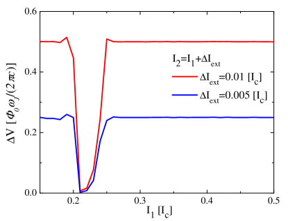
Figure 7: (color online) Voltage difference between two mesas $\Delta V=V_{2}-V_{1}$ when the mesas are biased by different current $I_{2}=I_{1}+\Delta I_{\rm{ext}}$.

Let us first consider two identical mesas with width $L=0.3\lambda_{c}$ and with a separation $L_{m}$. They locate at the position $L$ away from the edges of the base crystal. They are biased by the same current, $I_{1}=I_{2}=I_{\rm{ext}}$, as shown in Fig. 6(a). The results for different $L_{m}$ is shown in Fig. 5 . The main peak at the left side corresponds to the fundamental cavity mode of the mesa $\omega_{1}=\ell\pi/L$ and the the peak at the right side corresponds to the second cavity mode $\omega_{2}=2\ell\pi/L$. When the frequency of the plasma oscillations in the mesa matches the cavity frequency $\omega_{m}=m\ell\pi/L$, $|g_{j,L/R}|$ increases indicating a tendency of synchronization between two stacks. When $L_{m}=nL$, the phase coherence between different mesas becomes maximal. This becomes clearer for the second cavity mode, where two stacks do not synchronize at all when $L_{m}\neq nL$. For $L_{m}=0.7\lambda_{c}$, the peak at $I_{\rm{ext}}=2.0I_{c}$ is due to the cavity resonance inside the mesa. However the resonance occurs at smaller $I_{\rm{ext}}$ compared to that with $L_{m}=nL$. The downshift is due to the strong radiation damping through the base crystal as shown in Fig. 3.

The reasons for the better coherence when $L_{m}=nL$ are as follows. For the plasma oscillations uniform along the $c$ axis $q_{k}=0$, the in-plane dissipation is absent and the plasma is damped by the weak dissipation along the $c$-axis according to Eq. (7). However, for nonuniform oscillations with a finite wavenumber $q_{k}$, the in-plane dissipation becomes dominant for $N_{m}\approx 10^{3}$, and the nonuniform plasma oscillations in the base crystal decays quickly. Therefore the interaction between two mesas is weak and the synchronization becomes difficult. When $L_{m}=nL$, uniform cavity modes $q_{k}=0$ are possible as shown in Fig. 6 (a) and (b). Two mesas then are strongly coupled through the base crystal and they are synchronized. When $L_{m}\neq nL$, only nonuniform modes can be excited and the plasma oscillations in the base crystal is strongly damped by the in-plane dissipation. The amplitude of plasma oscillations is small compared to that when $L_{m}=nL$, see Fig. 6(c) and (d). Thus synchronization between mesas is hard to attain. Therefore the maximal synchronization is achieved when the position and size of mesas are commensurate with the standing wave in the base crystal, because the nonuniform plasma oscillations decay quickly in the base crystal.

Let us consider the phase shift of the gauge invariant phase difference between edges of mesas. As shown in Fig. 6(a), the supercurrent changes sign from the left edge to the right edge in the same mesa. This indicates there is a $\pi$ phase jump at the center of the mesa, and the $\pi$ phase kink is excited at the cavity resonanceLin and Hu (2008); Koshelev (2008). The $\pi$ phase kink helps to pump energy into the plasma oscillations and the amplitude of the oscillations is enhanced sharply at the cavity resonances, as described by the term at the right-hand side of Eq. (3). In Fig. 6(a) and (b), the plasma oscillations at the left/right edges have the same phase between different stacks when $L_{m}=(2n+1)L$. For $L_{m}=2nL$, there is $\pi$ phase shift between two mesas to match the standing wave in the base crystal.

In Fig. 7, the voltage of mesas with $L_{m}=L$ when they are biased by different current $I_{2}=I_{1}+\Delta I_{\rm{Iext}}$ is shown. At the cavity resonance when two mesas are synchronized, they have the same voltage despite that they are biased by slightly different current. Away from the cavity resonance, two mesas decouple from each other and they oscillate at different frequency.

V Conclusions

We have investigated the synchronization of mesa array through the plasma oscillations in the base crystal. If one regards the mesa arrays and base crystal as a whole, the plasma oscillations inside depends on the configuration of mesa arrays as a result of geometrical resonance. The amplitude of the plasma oscillations and the tendency of synchronization is governed by the dissipation of the whole system, hence is determined by the configuration of mesa array. When the period of mesa array $a$ close to the multiple integer of the mesa width $L$, $a\approx nL$, the dissipation is minimized and mesas are synchronized at cavity resonances of the whole system. Alternatively, one may treat mesa and base crystal separately. When the cavity resonance of mesa matches of that in the base crystal, mesa array is synchronized. Otherwise, the cavity resonance of the mesas is suppressed by the strong dissipation due to the radiation into the base crystal, and the mesa array is not synchronized. Therefore the optimal configuration for synchronization is $a\approx nL$. The above picture is corroborated by both analytical calculations and numerical simulations.

Acknowledgements –The authors thanks T. M. Benseman, U. Welp, and L. N. Bulaevskii for helpful discussions. SZL gratefully acknowledges funding support from the Office of Naval Research via the Applied Electrodynamics collaboration. AEK is supported by UChicago Argonne, LLC, operator of Argonne National Laboratory, a US DOE laboratory, operated under contract No. DE-AC02-06CH11357.

References

- Yanson et al. (1965) I. K. Yanson, V. M. Svistunov, and I. M. Dmitrenko, Zh. Eksp. Teor. Fiz. 48, 976 (1965).
- Dayem and Grimes (1966) A. H. Dayem and C. C. Grimes, Appl. Phys. Lett. 9, 47 (1966).
- Zimmerma.Je et al. (1966) Zimmerma.Je, J. A. Cowen, and A. H. Silver, Appl. Phys. Lett. , 353 (1966).
- Finnegan and Wahlsten (1972) T. F. Finnegan and S. Wahlsten, Appl. Phys. Lett. 21, 541 (1972).
- Jain et al. (1984) A. K. Jain, K. K. Likharev, J. E. Lukens, and J. E. Sauvageau, Phys. Rep. 109, 309 (1984).
- Darula et al. (1999) M. Darula, T. Doderer, and S. Beuven, Supercond. Sci. Technol. 12, R1 (1999).
- Barbara et al. (1999) P. Barbara, A. B. Cawthorne, S. V. Shitov, and C. J. Lobb, Phys. Rev. Lett. 82, 1963 (1999).
- Song et al. (2009) F. Song, F. M¨¹ller, R. Behr, and A. M. Klushin, Appl. Phys. Lett. 95, 172501 (2009).
- Kleiner et al. (1992) R. Kleiner, F. Steinmeyer, G. Kunkel, and P. Müller, Phys. Rev. Lett. 68, 2394 (1992).
- Hu and Lin (2010) X. Hu and S. Z. Lin, Supercond. Sci. Technol. 23, 053001 (2010).
- Savel’ev et al. (2010) S. Savel’ev, V. A. Yampol’skii, A. L. Rakhmanov, and F. Nori, Rep. Prog. Phys. 73, 026501 (2010).
- Iguchi et al. (2000) I. Iguchi, K. Lee, E. Kume, T. Ishibashi, and K. Sato, Phys. Rev. B 61, 689 (2000).
- Batov et al. (2006) I. E. Batov, X. Y. Jin, S. V. Shitov, Y. Koval, P. Müller, and A. V. Ustinov, Appl. Phys. Lett. 88, 262504 (2006).
- Bae et al. (2007) M. H. Bae, H. J. Lee, and J. H. Choi, Phys. Rev. Lett. 98, 027002 (2007).
- Benseman et al. (2011) T. M. Benseman, A. E. Koshelev, K. E. Gray, W.-K. Kwok, U. Welp, K. Kadowaki, M. Tachiki, and T. Yamamoto, Phys. Rev. B 84, 064523 (2011).
- Tachiki et al. (1994) M. Tachiki, T. Koyama, and S. Takahashi, Phys. Rev. B 50, 7065 (1994).
- Koyama and Tachiki (1995) T. Koyama and M. Tachiki, Solid State Commun. 96, 367 (1995).
- Tachiki et al. (2005) M. Tachiki, M. Iizuka, K. Minami, S. Tejima, and H. Nakamura, Phys. Rev. B 71, 134515 (2005).
- Bulaevskii and Koshelev (2006a) L. N. Bulaevskii and A. E. Koshelev, J. of Supercond. Novel Magn. 19, 349 (2006a).
- Bulaevskii and Koshelev (2007) L. N. Bulaevskii and A. E. Koshelev, Phys. Rev. Lett. 99, 057002 (2007).
- Lin et al. (2008) S. Z. Lin, X. Hu, and M. Tachiki, Phys. Rev. B77, 014507 (2008).
- Koshelev and Bulaevskii (2008) A. E. Koshelev and L. N. Bulaevskii, Phys. Rev. B 77, 014530 (2008).
- Tachiki et al. (2009) M. Tachiki, S. Fukuya, and T. Koyama, Phys. Rev. Lett. 102, 127002 (2009).
- Lin and Hu (2009) S. Z. Lin and X. Hu, Phys. Rev. B 79, 104507 (2009).
- Ozyuzer et al. (2007) L. Ozyuzer, A. E. Koshelev, C. Kurter, N. Gopalsami, Q. Li, M. Tachiki, K. Kadowaki, T. Yamamoto, H. Minami, H. Yamaguchi, T. Tachiki, K. E. Gray, W. K. Kwok, and U. Welp, Science 318, 1291 (2007).
- Kadowaki et al. (2008) K. Kadowaki, H. Yamaguchi, K. Kawamata, T. Yamamoto, H. Minami, I. Kakeya, U. Welp, L. Ozyuzer, A. Koshelev, C. Kurter, K. Gray, and W.-K. Kwok, Physca C 468, 634 (2008).
- Wang et al. (2009) H. B. Wang, S. Guénon, J. Yuan, A. Iishi, S. Arisawa, T. Hatano, T. Yamashita, D. Koelle, and R. Kleiner, Phys. Rev. Lett. 102, 017006 (2009).
- Wang et al. (2010) H. B. Wang, S. Guénon, B. Gross, J. Yuan, Z. G. Jiang, Y. Y. Zhong, M. Grunzweig, A. Iishi, P. H. Wu, T. Hatano, D. Koelle, and R. Kleiner, Phys. Rev. Lett. 105, 057002 (2010).
- Tsujimoto et al. (2010) M. Tsujimoto, K. Yamaki, K. Deguchi, T. Yamamoto, T. Kashiwagi, H. Minami, M. Tachiki, K. Kadowaki, and R. A. Klemm, Phys. Rev. Lett. 105, 037005 (2010).
- Tsujimoto et al. (2012) M. Tsujimoto, T. Yamamoto, K. Delfanazari, R. Nakayama, T. Kitamura, M. Sawamura, T. Kashiwagi, H. Minami, M. Tachiki, K. Kadowaki, and R. A. Klemm, Phys. Rev. Lett. 108, 107006 (2012).
- Yamaki et al. (2011) K. Yamaki, M. Tsujimoto, T. Yamamoto, A. Furukawa, T. Kashiwagi, H. Minami, and K. Kadowaki, Opt. Express 19, 3193 (2011).
- Lin and Hu (2008) S. Z. Lin and X. Hu, Phys. Rev. Lett. 100, 247006 (2008).
- Koshelev (2008) A. E. Koshelev, Phys. Rev. B 78, 174509 (2008).
- Lin and Hu (2012) S. Z. Lin and X. Hu, arXiv:1203.1375 (2012).
- Koshelev (2010) A. E. Koshelev, Phys. Rev. B 82, 174512 (2010).
- Orita et al. (2010) N. Orita, H. Minami, T. Koike, T. Yamamoto, and K. Kadowaki, Physica C 470, S786 (2010).
- Benseman et. al. (2012) T. M. Benseman et. al., to be published (2012).
- Koshelev and Bulaevskii (2009) A. E. Koshelev and L. N. Bulaevskii, J. Phys.: Conference Series 150, 052124 (2009).
- Sakai et al. (1993) S. Sakai, P. Bodin, and N. F. Pedersen, J. Appl. Phys. 73, 2411 (1993).
- Bulaevskii et al. (1994) L. N. Bulaevskii, M. Zamora, D. Baeriswyl, H. Beck, and J. R. Clem, Phys. Rev. B 50, 12831 (1994).
- Bulaevskii et al. (1996) L. N. Bulaevskii, D. Domínguez, M. P. Maley, A. R. Bishop, and B. I. Ivlev, Phys. Rev. B 53, 14601 (1996).
- Machida et al. (1999) M. Machida, T. Koyama, and M. Tachiki, Phys. Rev. Lett. 83, 4618 (1999).
- Koshelev and Aranson (2001) A. E. Koshelev and I. Aranson, Phys. Rev. B 64, 174508 (2001).
- Bulaevskii and Koshelev (2006b) L. N. Bulaevskii and A. E. Koshelev, Phys. Rev. Lett. 97, 267001 (2006b).