Collective Lyapunov modes

Abstract

We show, using covariant Lyapunov vectors in addition to standard Lyapunov analysis, that there exists a set of collective Lyapunov modes in large chaotic systems exhibiting collective dynamics. Associated with delocalized Lyapunov vectors, they act collectively on the trajectory and hence characterize the instability of its collective dynamics. We further develop, for globally-coupled systems, a connection between these collective modes and the Lyapunov modes in the corresponding Perron-Frobenius equation. We thereby address the fundamental question of the effective dimension of collective dynamics and discuss the extensivity of chaos in presence of collective dynamics.

1 Introduction

Emergence of collective behavior in large dynamical systems is a striking example of situations where microscopic interactions lead to non-trivial time-dependent macroscopic behavior, in contrast with equilibrium systems: a collection of dynamical units is in general not self-averaging, and hence macroscopic observables may show a variety of temporal evolutions even in the presence of microscopic chaos and in the absence of synchronization [1, 2, 3, 4]. Such non-trivial collective behavior (NTCB) is now known to be quite generic, being observed whether interactions are local or global, time variable is discrete or continuous [5, 6, 7, 8], and evolution is deterministic or noisy [9, 10, 11]. One of the most interesting features of NTCB is that microscopic chaos can coexist with macroscopic evolutions of different instability – periodic, quasi-periodic, and even chaotic in the case of global coupling [12, 4]. It is therefore natural to ask whether emerging macroscopic behavior can be captured by some of the Lyapunov exponents (LEs), which measure the infinitesimal rates of exponential divergence of nearby trajectories in phase space [13]. If such collective Lyapunov modes exist, they should shed light not only on how macroscopic and microscopic instabilities coexist in the single Lyapunov spectrum of the system, but also on a number of fundamental questions. For instance, the set of the collective LEs would give the effective dimension of the collective behavior and allow us to study its analogy to small dynamical systems, which had only been inferred so far from the observed dynamics. Furthermore, collective Lyapunov modes also call for redefining extensivity of chaos [14], which is usually taken to be the existence of a well-defined LE density per unit volume, numerically examined by measuring Lyapunov spectra at different system sizes and collapsing them after rescaling of the exponent index by the system size. Since NTCB is well-defined in the infinite-size limit, collective LEs characterizing NTCB are expected to be intensive, so that the above definition of the extensivity should not hold as it stands. Indeed, in contrast to spatiotemporal chaos in one spatial dimension, for which extensivity has been numerically shown in various generic models (see, e.g., [15, 16, 17]), in higher dimensions where NTCB can take place, only few studies could suggest extensivity [18, 19] within rather narrow ranges of system sizes.

Given this importance, a few earlier studies attempted to capture collective Lyapunov modes, without, however, reaching a definitive answer. Shibata and Kaneko [20] and, independently, Cencini et al. [21] argued that one needs to study finite-amplitude perturbations to quantify the instability of collective chaos in globally-coupled maps (see [22] for a review on such finite-size LEs). Showing that macroscopic instability is captured when the amplitude of the perturbation exceeds $\mathcal{O}(1/\sqrt{N})$, where $N$ is the system size, they implied that the standard LEs for infinitesimal perturbations do not reflect the collective dynamics. On the other hand, Nakagawa and Kuramoto studied a collective chaos regime of globally-coupled limit-cycle oscillators and showed that Lyapunov spectra at different system sizes overlapped onto each other, if a few LEs at both ends of the spectra were taken away before the spectra were rescaled by the system size [7]. They speculated that these LEs are associated with the collective dynamics, but they had to find such collective LEs by trial and error and, more importantly, could not provide any criterion to define them. Indeed, we and coworkers have recently shown that, for globally-coupled systems, in general, there are subextensive bands of LEs that should be scaled by $\log N$ instead of $N$ at both ends of the spectrum, which sandwich the extensive LEs in between [23]. Therefore, Nakagawa and Kuramoto may have actually taken away such subextensive LEs from the spectrum to obtain the remaining branch of extensive LEs, within the system sizes they studied, instead of truly collective Lyapunov modes.

This frustrating situation was overcome when Ginelli et al. proposed an efficient algorithm to compute covariant Lyapunov vectors (CLVs) in large dynamical systems [24, 25]. The CLVs are the vectors spanning the subspaces of the Oseledec decomposition of tangent space [13]. Each LE $\lambda^{(j)}$ has its associated CLV $\delta{\bi{x}}^{(j)}$ at any point on the trajectory ${\bi{x}}(t)$, which provides the intrinsic direction of perturbation growing at the rate $\lambda^{(j)}$. Therefore, the vector components of the CLVs indicate which dynamical units constitute the corresponding Lyapunov modes. Using this property of the CLVs, we, in our preceding work [26], reported numerical evidence that collective behavior of large dynamical systems is indeed encoded in their Lyapunov spectrum: while most modes are localized on a few degrees of freedom, thus corresponding to microscopic fluctuations of the system, there exist some collective modes characterized by the delocalized CLVs, acting therefore collectively on the dynamical units. The delocalization of the CLVs is quantified by the mean value of the inverse participation ratio (IPR) [27]

$$Y_{2}^{(j)}\equiv\Bigl{\langle}{\sum_{i}|\delta x_{i}^{(j)}|^{4}}\Bigr{\rangle}_{t},$$ (1)

where $\delta x_{i}^{(j)}$ is the $i$th component of the CLV $\delta{\bi{x}}^{(j)}$ normalized with the $L^{2}$-norm $\sum_{i}|\delta x_{i}^{(j)}|^{2}=1$ and the brackets $\langle\cdots\rangle_{t}$ indicate the average taken along the trajectory. Given that $Y_{2}$ provides the inverse of the average number of degrees of freedom participating in the mode $\delta{\bi{x}}^{(j)}$, we expect $Y_{2}\sim 1/N$ for the collective modes, as the number of the participating components increases with the system size $N$, while $Y_{2}$ stays constant for large $N$ for the remaining microscopic modes. This is our definition of the collective and microscopic modes, or the delocalized and localized modes, and provides a clear criterion for distinguishing them. In this way we indeed identified a few collective modes in collective chaos exhibited by globally-coupled limit-cycle oscillators [26]. We also showed, for globally-coupled maps with additive noise, that the collective modes in the standard Lyapunov analysis also arise as Lyapunov modes for the corresponding Perron-Frobenius dynamics, further justifying our definition of the collective modes.

This approach is further developed in the present article. After providing a detailed description on the detection of the collective modes in the limit-cycle oscillators, we shall study the role of each collective mode in the observed macroscopic dynamics (Section 2). Then, taking another, rather simple example of collective chaos in globally-coupled noisy maps, we show a quantitative correspondence between collective modes and Perron-Frobenius Lyapunov modes and discuss the generality of the role of the collective modes found in the preceding section (Section 3). On this basis, in Section 4, we study a regime of truly non-trivial collective chaos and show the interplay of macroscopic instabilities in this NTCB regime. We shall deal in particular with the effective dimension of collective chaos, revisiting earlier work by Shibata et al. [9] which concluded that the dimension $D$ increases as $D\sim-\log\sigma$ with decreasing noise amplitude $\sigma$ and hence the dimension is infinite in the noiseless limit $\sigma\to 0$. Here, we show how this dimension is related to the collective dynamics and to the macroscopic instabilities, and discuss the generality of our results. Section 5 is devoted to discussions and concluding remarks.

2 Existence of collective Lyapunov modes

We first demonstrate that the standard Lyapunov spectrum does contain collective Lyapunov modes, without the need to invoke finite-amplitude perturbations. Following Nakagawa and Kuramoto’s work [6, 7] and our preceding letter [26], we consider here $N$ globally-coupled limit-cycle oscillators

$$\dot{W}_{i}=W_{i}-(1+\mathrm{i}c_{2})|W_{i}|^{2}W_{i}+K(1+\mathrm{i}c_{1})(\langle W\rangle-W_{i}),$$ (2)

with $i=1,2,\cdots,N$, complex variables $W_{i}$, and the global field $\langle W\rangle\equiv\frac{1}{N}\sum_{i}W_{i}$. The parameter values are set to be $c_{1}=-2.0,c_{2}=3.0,K=0.47$, which correspond to a regime of collective chaos [6, 7, 26]. We numerically integrate Equation (2) by the fourth-order Runge-Kutta method with time step $0.1$ and compute LEs and CLVs using Ginelli et al.’s algorithm [24, 25]. Most data presented in this section are recorded over a period longer than $10^{5}$ after a transient of length $10^{4}$ or more is discarded. When full Lyapunov spectrum is computed, we allow a transient period of $100N$ or more for the convergence of the Lyapunov exponents and vectors.

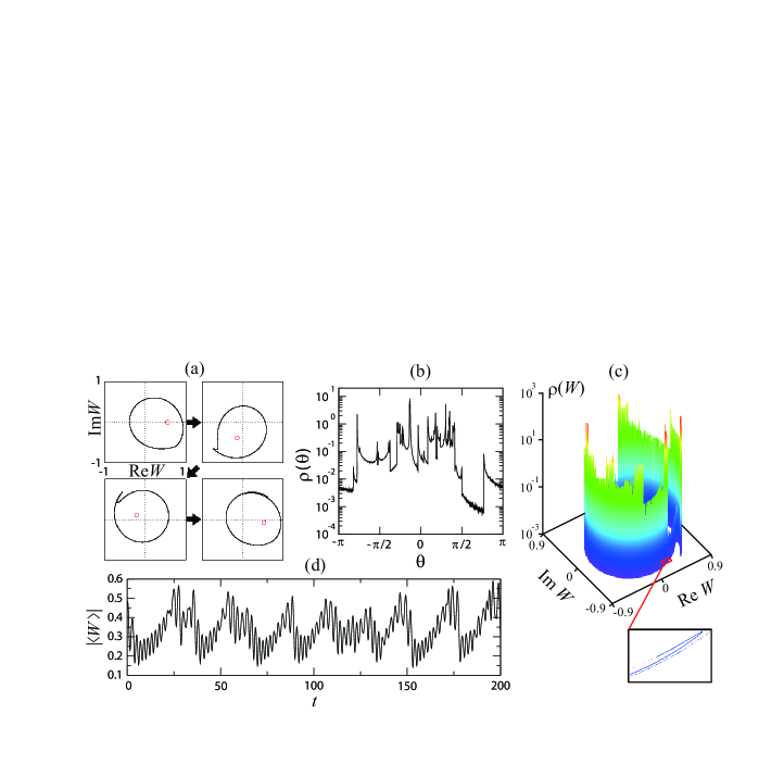
Figure 1: Collective chaos in $N=10^{7}$ globally-coupled limit-cycle oscillators (2). (a) Series of snapshots of the oscillators (dots) in the complex plane, taken at a fixed time interval $0.8$. The red circles indicate the position of the global field $\langle W\rangle$. (b) Typical instantaneous distribution for the angular position $\theta_{i}\equiv\arg W_{i}$ of the oscillators, here corresponding to the first snapshot in the panel (a). (c) Instantaneous distribution of the oscillators in the complex plane, at a moment near folding of the supporting line. The bottom panel shows the positions of the oscillators within the region indicated in the main panel. (d) Time series of the modulus of the global field, $|\langle W\rangle|$.

Collective chaos exhibited by these limit-cycle oscillators is shown in Figure 1. Because of the coupling to the global field, individual oscillators do not follow the limit-cycle oscillation but rotate rather irregularly with varying amplitudes and angular velocities, leading to stretching and folding of the supporting line (Figure 1(a)). This makes the local density of oscillators quite intricate with many peaks and fractal-like multilayer structure (Figure 1(b,c)). This imbalanced, fluctuating distribution of the oscillators drives irregular behavior of the global field $\langle W\rangle$ and other macroscopic variables, which, in the studied regime, takes the form of a weak chaotic modulation of a quasiperiodic signal as seen in the time series of the modulus, $|\langle W\rangle|$ (Figure 1(d)). This evolution resembles chaos emerging from a quasiperiodic regime in small systems such as in two coupled nonlinear oscillators with incommensurate frequencies [28].

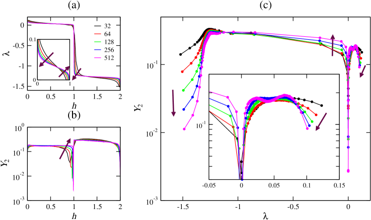
Figure 2: Spectra of LEs $\lambda^{(j)}$ against the rescaled index $h\equiv(j-0.5)/N$ (a), those of IPRs $Y_{2}^{(j)}$ (b), and the parametric plots $(\lambda^{(j)},Y_{2}^{(j)})$ (c), measured at different sizes $N$ for the globally-coupled limit-cycle oscillators (2). The arrows indicate increasing $N$. The insets show close-ups of the positive branch ($\lambda^{(j)}>0$) of the spectra.

The values of the LEs $\lambda^{(j)}$ and the IPRs $Y_{2}^{(j)}$ in this system are shown in Figure 2(a,b) against the rescaled index $h\equiv(j-0.5)/N$. Reflecting the LEs of an uncoupled limit-cycle oscillator, one zero and one negative, the Lyapunov spectra of the coupled system have two branches, near $0.05$ and $-1.25$ in this case (Figure 2(a)). The spectra at different sizes, however, do not collapse onto a single curve, but show rather strong size dependence (inset). This indicates that the system is not entirely extensive as expected for globally-coupled systems [23]. The spectra of the IPRs also tend to stay around some constant values within the two branches, indicating that most CLVs are localized according to our definition, but systematic drifts are also visible near both ends of the two branches (Figure 2(b)). The situation is better presented when the IPRs $Y_{2}^{(j)}$ are plotted against the corresponding LEs $\lambda^{(j)}$, as shown in Figure 2(c). Here we clearly see that $Y_{2}^{(j)}$ decreases with increasing $N$ at both ends of the spectra as well as near $\lambda^{(j)}=0$, while most Lyapunov modes are concentrated in the regions where the values of $Y_{2}^{(j)}$ hardly depend on $N$. This suggests that the Lyapunov spectra may contain delocalized, collective modes near the largest, smallest, and zero LEs, but not elsewhere for the system sizes studied here.

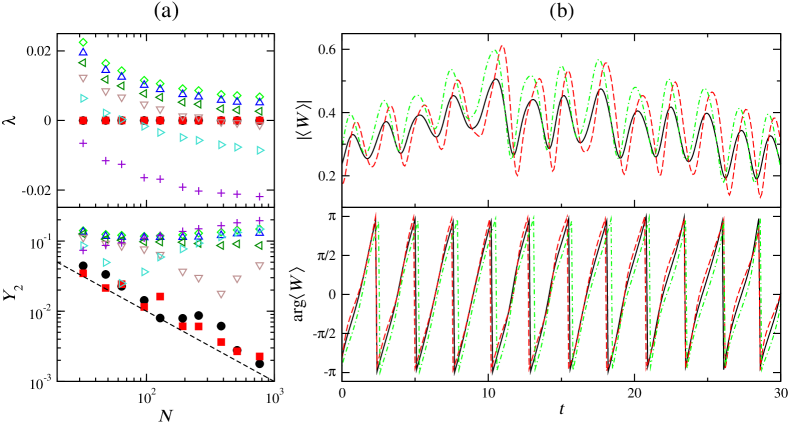
Figure 3: Collective modes at $\lambda^{(j)}=0$ in globally-coupled limit-cycle oscillators (2). (a) LEs $\lambda^{(j)}$ and IPRs $Y_{2}^{(j)}$ as functions of the system size $N$. The dashed line indicates $Y_{2}\sim 1/N$. The two neutral modes (solid symbols) are delocalized and thus collective, whereas other modes nearby (open symbols) are microscopic. (b) Time-series of the modulus and the argument of the global field $\langle W\rangle$ at $N=256$, for the unperturbed trajectory $\bi{W}$ (black solid line) as well as for the “perturbed ones” $\bi{W}+c_{1}\delta\bi{W}^{\mathrm{(zero1)}}$ (red dashed line) and $\bi{W}+c_{2}\delta\bi{W}^{\mathrm{(zero2)}}$ (greed dot-dashed line) with arbitrary constants $c_{1}$ and $c_{2}$. Here the former and the latter shift the phase for $|\langle W\rangle|$ and $\arg\langle W\rangle$, respectively, though in general these degenerated Lyapunov modes are arbitrary superpositions of the two fundamental perturbations.

Now we demonstrate that there indeed exist a few collective modes in these regions. Concerning the region near $\lambda^{(j)}=0$, the system has two neutral modes associated with invariance under time translation and angular rotation. They are delocalized and thus collective as their $Y_{2}^{(j)}$ decreases as $1/N$ (solid symbols in Figure 3(a)). Indeed, these collective modes shift the two phases of the quasiperiodic collective dynamics under the chaotic modulation, as shown in time series of the global field for the unperturbed trajectory $\bi{W}$ and for those shifted in the direction of the two corresponding CLVs, $\delta\bi{W}^{\mathrm{(zero1)}}$ and $\delta\bi{W}^{\mathrm{(zero2)}}$ (Figure 3(b)). In contrast, other nearby LEs change their values smoothly as $N$ is varied, some of them crossing the zero line (open symbols in Figure 3(a)). The IPRs of these modes are essentially independent of $N$, except when their LEs become accidentally close to zero, in which case the numerical scheme cannot resolve well the degeneracy with the collective zero modes. This clearly indicates that these near-zero modes are microscopic.

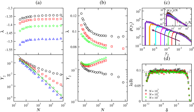
Figure 4: First and last Lyapunov modes in globally-coupled limit-cycle oscillators (2). (a,b) LEs $\lambda^{(j)}$ and IPRs $Y_{2}^{(j)}$ against the system size $N$, for the last four modes (a) and the first three modes (b). The dashed line in the panel (a) indicates $Y_{2}\sim 1/N$. (c) Histogram of the instantaneous IPR $y_{2}$ for the first mode, measured at $N=512,2048,\cdots,131072,10^{6},10^{7},5\times 10^{7}$ (increasing as indicated by the arrow). The abscissa is multiplied by $N$ in the inset. (d) Finite-size LE $\lambda(\delta)$ as a function of the amplitude $\delta$ of the perturbation. The dashed line shows the value of the largest LE $\lambda^{(1)}$ at $N=131072$.

For the negative end of the spectrum, Figure 4(a) shows the values of the LEs $\lambda^{(j)}$ and the IPRs $Y_{2}^{(j)}$ as functions of the system size $N$ for the last four modes. Although their IPR values decrease more slowly than $1/N$ for small system sizes, when $N$ is increased further, the last two modes become completely delocalized, i.e., $Y_{2}^{(j)}\sim 1/N$, whereas the IPRs of the other modes decrease more and more slowly towards some asymptotic non-zero values. Therefore, only the last two Lyapunov modes are collective here. The situation is similar at the positive end of the spectrum (Figure 4(b)), except that one needs to explore extremely large system sizes: the IPR of the first mode starts to decrease faster and faster only above $N=10^{6}$, and is still far from the $1/N$ decay at $N=5\times 10^{7}$. However, the histogram of the instantaneous values of the IPR, $y_{2}^{(1)}\equiv\sum_{i}|\delta W_{i}^{(1)}|^{4}$, reveals that the distribution function actually scales as $1/N$, except the upper bound which is fixed at $y_{2}^{(1)}=1$ by definition (Figure 4(c)). This indicates the asymptotic scaling of $Y_{2}^{(1)}\sim 1/N$ and therefore the first Lyapunov mode is collective. This conclusion can also be confirmed by using finite-amplitude perturbations. Shibata and Kaneko [20] and Cencini et al. [21] showed, somewhat speculatively, that the mean expansion rate $\lambda(\delta)$ of perturbations of size $\delta$, called the finite-size LE [22], are equal to the largest LE $\lambda^{(1)}$ for $\delta\ll\delta_{\rm c}\sim 1/N$ and to the largest expansion rate of the collective dynamics for $\delta\gg\delta_{\rm c}$. In our case, since the first mode is collective, the finite-size LE $\lambda(\delta)$ exhibits a single plateau at the value of the first LE $\lambda^{(1)}$ regardless of the system size $N$ (Figure 4(d)).

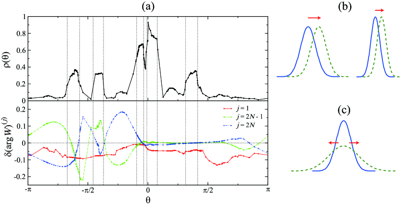
Figure 5: Role of the collective modes with positive and negative LEs ($j=1$ and $j=2N-1$ and $2N$, respectively) in the globally-coupled limit-cycle oscillators (2) at $N=512$. (a) Instantaneous profile for the density $\rho(\theta)$ of the oscillators (upper panel) and the shift in their angular positions induced by the collective Lyapunov modes, $\delta(\arg W_{i})^{(j)}$ (lower panel). The vertical dotted lines indicate the regions of the five main peaks in the density profile. The local density $\rho(\theta_{i})$ is measured from the number of oscillators within the range $[\theta_{i}-\pi/20,\theta_{i}+\pi/20]$. The profile of $\delta(\arg W_{i})^{(1)}$ is locally averaged with the same window, while the raw data are shown for $\delta(\arg W_{i})^{(2N-1)}$ and $\delta(\arg W_{i})^{(2N)}$. (b,c) Schematic drawings illustrating the role of the positive (b) and negative (c) collective modes.

The role of these three collective Lyapunov modes can also be studied from the structure of the corresponding CLVs. Although, strictly, the full structure of the CLVs as well as of the oscillator density in the complex plane should be considered, we have confirmed that the components of the CLVs for the collective modes are mostly along the supporting line of the oscillators, so that the vector structures can be faithfully represented on the angular coordinates, $\theta_{i}\equiv\arg W_{i}$. Figure 5(a) shows an instantaneous profile of the oscillator density $\rho(\theta)$ projected on the angular coordinates $\theta_{i}$ (upper panel) and the shift in the angular positions induced by each of the three collective modes with positive and negative LEs, $\delta(\arg W_{i})^{(j)}\equiv\lim_{\epsilon\to 0}[\arg(W_{i}+\epsilon\delta W_{i}^{(j)})-\arg W_{i}]/\epsilon=\mathrm{Im}(\delta W_{i}^{(j)}/W_{i}^{(j)})$ (lower panel). One can see that the shift due to the positive collective mode, $\delta(\arg W_{i})^{(1)}$ (red solid line), is varying along the angular coordinates, except in the peaked regions of the oscillator density (indicated by vertical dotted lines) where the values of $\delta(\arg W_{i})^{(1)}$ stay practically constant. This indicates that the positive collective mode moves these peaks in the density profile, almost uniformly, with different amplitudes (Figure 5(b)). Since such a shift makes a direct perturbation to the global field $\langle W\rangle$, which behaves chaotically in the present regime, this mode is naturally assigned with the positive LE $\lambda^{(1)}$. By contrast, for the two negative collective modes, the angular shifts $\delta(\arg W_{i})^{(2N-1)}$ and $\delta(\arg W_{i})^{(2N)}$ vary widely and often change their sign within the peaked regions (green dashed and blue dot-dashed lines). The two tails of the peaks are then moved in the opposite directions, and hence the peak widths are expanded or narrowed (Figure 5(c)). Since these modes have negative LEs, such perturbations leading to changes in the peak widths decay exponentially fast. In other words, these negative collective modes tend to adjust the width of the peaks, maintaining local synchronization of the oscillators. The two neutral collective modes have already been studied in Figure 3(b) and turned out to shift the two fundamental phases of the remaining quasiperiodic behavior.

To summarize, we have found one positive, two neutral, and two negative collective modes, at least up to the largest sizes we studied. This set of the collective LEs is analogous to small dynamical systems exhibiting bifurcation from quasiperiodic to chaotic behavior [28], but here the associated CLVs act on collections of oscillators, controlling dynamics of peaks in the density profile. We have shown, therefore, that collective Lyapunov modes do exist within the framework of the standard Lyapunov analysis, characterized by the delocalization of the CLVs, without the need to rely on finite-amplitude perturbations. Unlike the finite-amplitude perturbations which capture the largest expansion rate in the collective dynamics, the collective Lyapunov modes characterize, we believe, full instability that emerges at the collective level. However, we have also noticed that we need to overcome strong finite-size effects, in order for collective modes to be clearly decoupled from neighboring microscopic modes (see Figure 4(a,b)), which is unfortunately quite demanding with the current machine power. The situation becomes even worse for locally coupled systems such as coupled map lattices, for which one needs at least two spatial dimensions to study NTCB [1] and, further, local correlation of dynamical units reduces the effective system size, though we believe that collective Lyapunov modes should exist in locally-coupled systems as well. In addition, for globally-coupled systems, the existence of collective chaos also helps us to capture collective Lyapunov modes, since for large system sizes one can typically probe only first few Lyapunov modes with positive LEs. Moreover, globally-coupled systems allow us to investigate the infinite-size limit “directly” from the evolution of the instantaneous density profile, which is given by the nonlinear Perron-Frobenius (PF) equation [3, 9, 4]. Lyapunov exponents measured in the PF dynamics have therefore been related to the collective dynamics [4], without, however, direct evidence being ever shown. In the next section, following our preceding letter [26], we will show that there is indeed a quantitative correspondence between the collective Lyapunov modes and some of such PF Lyapunov modes.

3 Correspondence to Perron-Frobenius Lyapunov modes

The PF equation describes the evolution of the instantaneous distribution function of the dynamical variables, denoted here by $\rho^{t}(x)$. This idea can be applied to a single dynamical unit for globally-coupled systems, since the global field is given by $\rho^{t}(x)$, which makes the PF equation nonlinear [3, 9, 4]. Then, one needs to rely on numerical approaches in most cases, typically discretizing the support of the evolving distribution into sufficiently fine bins. It is unfortunately unrealistic for the globally-coupled limit-cycle oscillators studied above, because of the intricate, fractal-like structure of the support in the complex plane (see Figure 1(c)). To avoid this difficulty, we study here a simpler case of globally-coupled maps of a real variable, whose support is typically a bounded interval of the real axis.

Specifically, we consider the following system:

$$x_{i}^{t+1}=(1-K)f(x_{i}^{t})+K\langle f(x)\rangle+\xi_{i}^{t},$$ (3)

with the logistic map $f(x)=1-ax^{2}$ and an iid noise $\xi_{i}^{t}$, which is added here to avoid singularities in the PF dynamics as explained below. In the infinite-size limit $N\to\infty$, the corresponding nonlinear PF equation reads

$$\rho^{t+1}(x)=\int\rho_{\rm N}(F^{t}(y)-x)\rho^{t}(y)\mathrm{d}y,$$ (4)

where $\rho_{\rm N}(\xi)$ is the probability density of the noise and

$$F^{t}(y)=(1-K)f(y)+K\int f(z)\rho^{t}(z)\mathrm{d}z.$$ (5)

If the system is noiseless, i.e., if $\xi_{i}^{t}=0$, $\rho_{\rm N}(\xi)$ is replaced by the delta function and hence

$$\rho^{t+1}(x)=\frac{1}{1-K}\sum_{\textrm{\scriptsize$y$ s.t. $F^{t}(y)=x$}}\frac{\rho^{t}(y)}{|f^{\prime}(y)|},\quad(\textrm{if noiseless}),$$ (6)

where the summation is taken over the preimages of $x$ and $f^{\prime}(y)$ is the first derivative of $f(y)$. Following these preimages and dealing with the singularity due to the superstable point $f^{\prime}(y)=0$ make the system practically inaccessible by numerical means. This singularity is tamed by adding noise to the system as in Equation (3), or by studying a heterogeneous system with site-dependent local parameters [20, 21], which do not destroy collective dynamics but provides a useful situation to elucidate the nature of the collective behavior [9, 10, 11].

Computation of the PF equation (4) and its tangent space dynamics is straightforward, but has a few pitfalls which have been overlooked by some earlier studies. First, the noise distribution $\rho_{\rm N}(\xi)$ must be bounded in such a way that the distribution of the dynamical units, $\rho^{t}(x)$, is always confined within the basin of attraction. Gaussian noise cannot be used here for this reason. Second, because the tangent space dynamics reads

$$\delta\rho^{t+1}(x)=\int\mathrm{d}y\left[\rho_{\rm N}(F^{t}(y)-x)\delta\rho^{t}(y)+K\rho^{\prime}_{\rm N}(F^{t}(y)-x)\rho^{t}(y)\int f(z)\delta\rho^{t}(z)\mathrm{d}z\right]$$ (7)

and involves the derivative of $\rho_{\rm N}(\xi)$, the noise distribution must be differentiable for proper computation of LEs and CLVs. For these reasons, we choose the Kumaraswamy noise distribution [29] $\rho_{\rm N}(\xi)=\alpha\beta(\xi^{\prime})^{\alpha-1}(1-(\xi^{\prime})^{\alpha})^{\beta-1}$ with $\xi^{\prime}\equiv(\xi/\sigma+1)/2\in[0,1]$, $\alpha=3$, and $\beta=5$, for which the probability density is unimodal, bounded within $\xi\in[-\sigma,\sigma]$, twice differentiable, and nearly symmetric.

We start with a rather simple regime of collective chaos under strong coupling, where dynamical variables tend to synchronize to the chaotic dynamics of the uncoupled logistic map, but are weakly scattered by microscopic chaos and noise [10, 11, 30]. Specifically, we set the local logistic parameter at $a=1.57$, which corresponds to the one-band chaos regime, and in the present section $K=0.28$ and $\sigma=0.1$, unless otherwise specified. We perform both direct simulations of the maps (3) with finite $N$ and simulations of the PF equation (4), which should correspond to the $N\to\infty$ limit. It is indeed checked by confirming that the evolution of $\rho^{t}(x)$ from the PF equation matches that of large collections of the maps for many time steps, when starting from almost identical initial density profiles. In the following, we compare Lyapunov modes obtained by the two methods. Most data are recorded over $3\times 10^{5}$ time steps after a transient period of $300N$ or $50000$ steps for the maps, and recorded over $10^{5}$ steps after discarding $10^{4}$ steps for the PF equation, simulated with sufficiently many bins of equal width (typically 1024 bins within the interval $[-1.0,1.5]$ in this section).

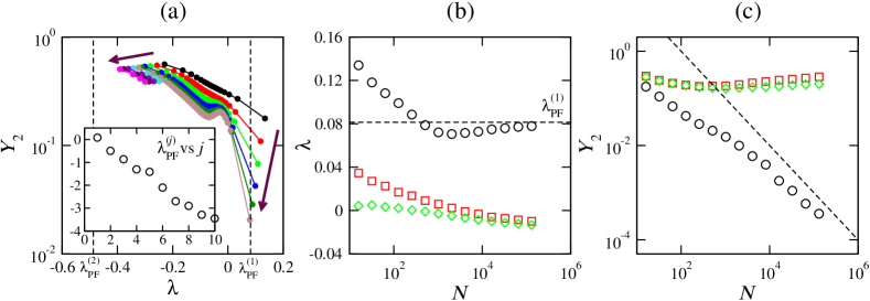
Figure 6: Lyapunov analysis for globally-coupled noisy logistic maps (3) with $a=1.57,K=0.28,\sigma=0.1$ and the corresponding PF equation (4). (a) IPR $Y_{2}^{(j)}$ against LE $\lambda^{(j)}$ for the maps with $N=16,32,\cdots,512$. The last four modes are shown additionally for $N=2048,8192,\cdots,131072$. The arrows indicate increasing $N$. The inset shows the spectrum of LEs for the PF dynamics, $\lambda_{\rm PF}^{(j)}$. The values of the first and second PF LEs, namely $\lambda_{\rm PF}^{(1)}=0.081$ and $\lambda_{\rm PF}^{(2)}=-0.49$, are indicated by the vertical dashed lines in the main panel. (b,c) First three LEs (b) and their IPRs (c) as functions of the size $N$ of the maps. The dashed line in the panel (b) indicates the value of the first PF LE $\lambda_{\rm PF}^{(1)}$ and that in the panel (c) indicates $Y_{2}\sim 1/N$.

Figure 6(a) displays the full parametric plots of $(\lambda^{(j)},Y_{2}^{(j)})$ for the maps up to $N=512$, showing signs of delocalization for first few modes. Increasing the system size further, we find that only the first one is actually delocalized, i.e., $Y_{2}^{(1)}\sim 1/N$, while the following ones are localized (Figure 6(c)). The values of the LEs also vary differently for the first mode, which remains well separated from the others irrespective of the size $N$ (Figure 6(b)). Moreover, comparison to the LEs for the PF equation reveals that this first, collective LE tends to the first PF LE, suggesting $\lim_{N\to\infty}\lambda^{(1)}=\lambda_{\rm PF}^{(1)}$. For the following Lyapunov modes, however, we do not find such direct correspondence within the system sizes probed here. The PF LEs $\lambda_{\rm PF}^{(j)}$ decrease so rapidly with increasing index $j$ (Figure 6(a) inset) that even the second one $\lambda_{\rm PF}^{(2)}$ is smaller than the last LE of the maps, $\lambda^{(N)}$ (main panel). The values of the last few LEs decrease as the system size increases, but they do not reach $\lambda_{\rm PF}^{(2)}$ nor indicate any sign of delocalization in the associated IPRs up to the largest size we examined, namely $N=131072$. The first Lyapunov mode is therefore the only collective mode present at the studied system sizes, so that it takes the same LE value as the first PF Lyapunov mode.

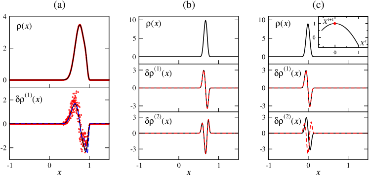
Figure 7: Snapshots of the distribution $\rho(x)$ and CLVs $\delta\rho^{(j)}(x)$ for globally-coupled noisy logistic maps (3) with $a=1.57$. (a) Typical snapshots for $K=0.28$ and $\sigma=0.1$. Black solid lines and red circles indicate the results from PF and the maps of size $N=10^{7}$, respectively. The blue dashed line shows the (normalized) first derivative of $\rho(x)$, which overlaps the PF CLV $\delta\rho^{(j)}(x)$ for the most part. (b,c) Snapshots for $K=0.70$ and $\sigma=0.1$, taken at a typical moment (b) or when the global field $X^{t}\equiv\langle x^{t}\rangle$ is near the superstable point (c). The black solid lines indicate the results from PF, whereas the red dashed lines show the $j$th derivative of $\rho(x)$. The inset of the panel (c) shows the return map of the global field, the red point indicating the moment when the snapshots are taken.

The correspondence between this collective mode and the first PF Lyapunov mode is underpinned from the structure of their CLV. Figure 7(a) compares the distribution $\rho(x)$ (top panel) and the first CLV $\delta\rho^{(1)}(x)$ (bottom panel) obtained directly from the PF equation (black solid line) and those constructed from the maps of size $N=10^{7}$ (red circles), at a moment when the two distributions coincide very well. One can see that the first CLV from the maps exerts the same shift $\delta\rho^{(1)}(x)$ on the distribution as that from the PF equation (bottom panel). It indicates that this collective mode, identified in the original system by the standard Lyapunov analysis, should indeed converge to the PF Lyapunov mode in the infinite-size limit. Moreover, we notice in Figure 7(a) that the spatial profile of the CLV $\delta\rho^{(1)}(x)$ is very close to the first derivative of the distribution, $\partial_{x}\rho(x)$ (blue dashed line), which is normalized here with the same $L^{2}$-norm as the CLV. Since $\rho(x+\Delta x)\simeq\rho(x)+\partial_{x}\rho(x)\Delta x$ for small $\Delta x$, this collective mode with the positive LE merely shifts the position of the peak, similarly to the positive collective mode found in the globally-coupled limit-cycle oscillators (see Figure 5).

The similarity to the derivative is more prominent for larger coupling strengths $K$. For $K=0.70$, the first PF CLV $\delta\rho_{\rm PF}^{(1)}(x)$ and the first derivative $\partial_{x}\rho(x)$ are almost indistinguishable, and, actually, so are the $j$th PF CLV $\delta\rho_{\rm PF}^{(j)}(x)$ and the $j$th derivative $\partial_{x}^{j}\rho(x)$ for most times (Figure 7(b)), unless $j$ is too large. In particular, the second PF CLV $\delta\rho_{\rm PF}^{(2)}(x)$ resembles the second derivative $\partial_{x}^{2}\rho(x)$, which can be regarded as the “diffusion term” that changes the width of the peak. The associated LE being negative, $\lambda_{\rm PF}^{(2)}=-1.69$ here, this second PF Lyapunov mode maintains a constant width of the peak for each moment of the evolution. This is again similar to the negative collective modes in the limit-cycle oscillators, though the second PF mode in the present system is not captured by the Lyapunov analysis of the maps at least for the studied system sizes. The similarity of the $j$th CLV to the $j$th derivative is, however, lost occasionally, when the global field $X^{t}\equiv\langle x^{t}\rangle$ visits the close vicinity of the superstable point in its return map (Figure 7(c); recall that the global field evolves like a single uncoupled logistic map in this case). Then, since $F^{t}(y)$ in Equation (5) hardly depends on $y$, Equation (4) merely yields $\rho^{t+1}(x)\approx\rho_{\rm N}(1-x)$ irrespective of $\rho^{t}(x)$. This results in the near degeneracy of all the CLVs, as indicated in Figure 7(c).

In this section, we have shown a quantitative correspondence between a collective Lyapunov mode identified for the maps and a Lyapunov mode of the corresponding PF dynamics, both having the same value of the LE and applying the same perturbation to the collection of the dynamical units in the infinite-size limit. The correspondence has been demonstrated for the (single) positive Lyapunov mode in the strong-coupling regime of the globally-coupled noisy logistic maps, whereas we could not capture a PF Lyapunov mode with negative LE by analyzing the maps, for the system sizes probed in the present study. In fact, we consider that negative Lyapunov modes in the PF representation may not necessarily be present in the original dynamical systems. A trivial example is an uncoupled collection of identical chaotic maps, e.g., at $K=0$ for the current system (3), where all Lyapunov modes are degenerate at the single positive LE, while the PF dynamics yields infinitely many negative LEs. These negative PF modes should correspond to superpositions of local perturbations to the local maps, so that the perturbation grows exponentially in phase space but the perturbed distribution relaxes towards the invariant measure. In contrast, we believe that PF modes with zero or positive LE should be all present as collective modes in the original system, because they cannot be superpositions of such incoherent microscopic perturbations. Similarly, we conjecture that all collective modes in dynamical systems should also arise in the corresponding PF equations, regardless of the sign of the LEs, because our definition of the collective modes indicates that $\mathcal{O}(N)$ dynamical units are perturbed thereby, which should also have impacts on the distribution. A question that may naturally arise here is whether one can distinguish such “physical” PF Lyapunov modes from “spurious” ones, which are missing in the original dynamical systems, among infinitely many negative PF LEs. Hyperbolicity of the Lyapunov modes could be a key to tackle this problem, as in spatially-extended dissipative systems where the Lyapunov spectrum consists of a finite number of mutually connected physical modes and the remaining spurious modes that are hyperbolically decoupled from all the physical modes [31, 32], but first attempts in this direction worked only for the trivial case of the fully synchronized collective chaos (data not shown). Elucidating this possible decoupling of the physical and spurious PF Lyapunov modes for general cases of NTCB is a fundamental issue left for future studies.

4 Dimension and nature of non-trivial collective chaos

The study in the previous section allowed us to establish the direct connection between a collective mode and a PF Lyapunov mode, but we dealt with a rather trivial regime of collective behavior with strong coupling, which reduces for $K=0.70$ to the fully synchronized state of the local maps in the noiseless limit. Now we turn our attention to a regime of non-trivial collective chaos, where dynamical units loosely form a number of coevolving clusters, mutually connected and interacting through chaotic behavior of the global field. We focus in particular on a weak-coupling regime of the globally-coupled noisy logistic maps (3) with $a=1.86$ and $K=0.10$, studied earlier by Shibata et al. [9]. They measured the Kaplan-Yorke dimension $D_{\rm KY}$ from the PF LEs and found it to grow with decreasing noise amplitude $\sigma$ as $D_{\rm KY}\sim-\log\sigma$, using however the Gaussian noise distribution, for which one cannot numerically evolve the PF equation (4) in a proper way. Here, using the controlled Kumaraswamy noise with various amplitudes, we revisit this problem of the effective dimension and, moreover, examine the instabilities of collective chaos on the basis of the Lyapunov approach developed in the previous sections. The transient and recording periods are typically $300N$ and $3\times 10^{5}$ time steps for the maps and $10^{4}$ and $10^{5}$ time steps for the PF equation, respectively.

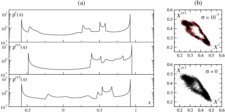
Figure 8: Collective chaos dynamics in globally-coupled noisy logistic maps (3) with $a=1.86$ and $K=0.10$. (a) Three consecutive snapshots of the instantaneous distribution $\rho^{t}(x)$ for $\sigma=1\times 10^{-3}$, obtained from the evolution of the PF equation (4) with $65536$ bins. (b) Return maps of the global field $X^{t}\equiv\langle x^{t}\rangle$ for $\sigma=1\times 10^{-3}$ (top) and $\sigma=0$ (bottom). The black and red dots indicate the results from $10^{7}$ maps and the PF equation, respectively.

Figure 8(a) shows the time evolution of the instantaneous distribution $\rho^{t}(x)$ in this regime, with noise amplitude $\sigma=1\times 10^{-3}$. The distribution now consists of a number of peaks, connected to each other by gradually varying low-density regions, in striking contrast to the strong-coupling regime (Figure 7(a)) but rather similarly to the collective chaos in the limit-cycle oscillators (Figure 1(b)). Here, on top of the broad support, the rightmost, sharpest peak is created from the superstable point of $F^{t-1}(y)$, i.e., $y=0$ (see Equation (5)); its image would be singular if no noise were added, but in the presence of noise it is scattered and leaves a peak of finite width, roughly $\sigma$. This peak is then transported to different positions on each time step, with its width broadened by noise and chaos, and is finally dispersed over the support. Because of this intricate structure of the distribution, the return map of the global field $X^{t}\equiv\langle x^{t}\rangle$ is not simple and single-valued any more (Figure 8(b) top panel), being scattered around the mean values. This readily suggests that the effective dimension of the collective chaos is not as low as in the strong-coupling case. Somewhat counterintuitively, eliminating the noise does not reduce this scattering but, instead, enhances it (Figure 8(b) bottom panel), because the noise smooths the intricate structure of the distribution $\rho^{t}(x)$ and simplifies the collective dynamics. The noise also allows us to simulate the evolution of $\rho^{t}(x)$ precisely by the PF equation with finite numbers of bins: for $\sigma=1\times 10^{-3}$, for example, a large collection of maps and the PF equation yield statistically indistinguishable results for the return map (Figure 8(b) top panel).

The Lyapunov spectrum of this system at $\sigma=1\times 10^{-3}$ is measured both from the maps (Figure 9(a,b)) and from the PF equation (black circles in Figure 10(a)). One notices that, in this weak-coupling regime, even the largest LE in the PF dynamics, $\lambda_{\rm PF}^{(1)}\approx 0.047$, is much smaller than all the LEs in the maps with finite $N$ we investigated. Indeed, none of the Lyapunov modes from the maps show signs of delocalization (Figure 9(b)): the local minimum of $Y_{2}^{(j)}$ apparent in Figure 9(b) depends only weakly on $N$, specifically $Y_{2}^{(j_{\rm min})}\sim N^{-0.35}$ in contrast to $Y_{2}\sim 1/N$ for the true delocalization, even in the distribution of the instantaneous IPR values $y_{2}$ (Figure 9(c); to be compared with Figure 4(c) for the case of a true collective mode). This local minimum is actually due to the near degeneracy of LEs around $\lambda^{(j)}\approx 0.34$ (Figure 9(a)), which is typical of globally-coupled systems [23] and thus also present in Figures 2 and 6(a). Although the eventual emergence of collective modes is expected somewhere in the spectrum, which tends to cover a wider range of LE values for larger $N$, their detection seems out of reach of current computer power. We therefore focus on the PF Lyapunov modes in the following, to investigate the nature of the non-trivial collective chaos.

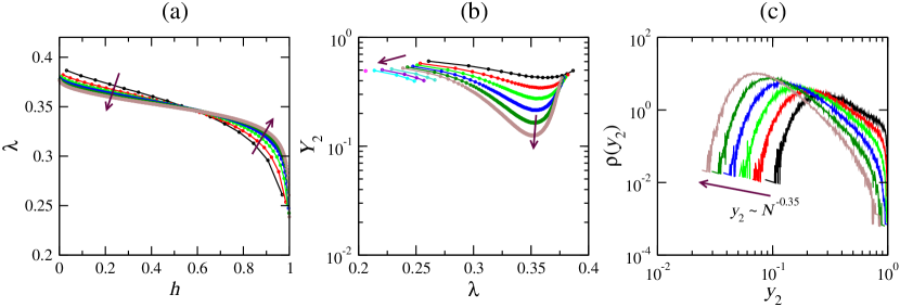
Figure 9: Lyapunov spectrum of the maps with finite $N$ for globally-coupled noisy logistic maps (3) with $a=1.86$, $K=0.10$, and $\sigma=1\times 10^{-3}$. (a) LE $\lambda^{(j)}$ vs rescaled index $h\equiv(j-0.5)/N$ and (b) parametric plots $(\lambda^{(j)},Y_{2}^{(j)})$ for $N=16,32,\cdots,512$ (increasing as indicated by the arrows). The last four modes are shown additionally for $N=2048,8192,32768$ and the last mode is shown for $N=131072$. (c) Distribution of the instantaneous IPR $y_{2}^{(j_{\rm min})}$ for the mode at the local minimum in the panel (b), $j_{\rm min}\equiv\arg\min Y_{2}^{(j)}$.

Figure 10: Lyapunov spectrum of the PF equation for globally-coupled noisy logistic maps (3) with $a=1.86$ and $K=0.10$. (a) PF Lyapunov spectrum $\lambda_{\rm PF}^{(j)}$ for various noise amplitudes $\sigma=1\times 10^{-3},4\times 10^{-4},2\times 10^{-4},1\times 10^{-4},4\times 10^{-5}$ (from bottom to top). Sufficiently many bins are used in order that the shown values of the LEs are reliable. The arrow indicates a rough position of the threshold between the two regions, for $\sigma=1\times 10^{-3}$ (see text). Inset: Kaplan-Yorke dimension $D_{\rm KY}$ and the index of the inflection point $j_{\rm inf}$ as functions of $\sigma$. (b) The first three PF LEs as functions of $\sigma$ (inset) and $\sigma^{1/4}$ (main panel). The dashed lines indicate the best linear fits to the data for $\sigma\leq 4\times 10^{-4}$. (c) $(\lambda_{0}-\lambda_{\rm PF}^{(j)})\sigma^{-1/4}$ against $j$ (same symbols as in (a)) with $\lambda_{0}=0.163$. The dashed line shows an estimate of the asymptotic curve $F_{j}$, obtained by a quadratic fit to the data for $\sigma=4\times 10^{-5}$ (green leftwards triangles) within $j\leq 17$.

The PF Lyapunov spectrum consists of gradually descending LEs, showing, roughly, two different slopes for the beginning and the rest of the spectrum, as indicated by the arrow in Figure 10(a) for $\sigma=1\times 10^{-3}$. With decreasing noise amplitude $\sigma$, both negative slopes increase and the threshold between the two regions shifts rightwards. This obviously increases the value of the Kaplan-Yorke dimension $D_{\rm KY}$, which turns out to grow as $D_{\rm KY}\sim-\log\sigma$ for small $\sigma$ (black circles in the inset) similarly to the result by Shibata et al. [9]. In fact, the position of the threshold also moves logarithmically, as indicated by the index of the inflection point of the spectrum, $j_{\rm inf}$ (red squares in the inset). In contrast, the values of the LEs $\lambda_{\rm PF}^{(j)}$ with fixed indices cannot increase logarithmically, since they should remain finite in the noiseless limit. Instead, our data suggest that at least first few LEs depend linearly on $\sigma^{1/4}$, i.e., $\lambda_{\rm PF}^{(j)}\simeq\lambda_{0}-F_{j}\sigma^{1/4}$ (Figure 10(b)). Moreover, the estimates of $\lambda_{0}$ from the fits to the first three LEs (dashed lines) coincide very well at $\lambda_{0}=0.163(1)$, where the number in the parentheses indicates a range of error in the last digit. Rescaling the Lyapunov spectra in Figure 10(a) as $(\lambda_{0}-\lambda_{\rm PF}^{(j)})\sigma^{-1/4}$ with the above estimate of $\lambda_{0}$, we find a reasonable collapse for small $j$ (Figure 10(c)), which indicates that the asymptotic behavior $\lambda_{\rm PF}^{(j)}\simeq\lambda_{0}-F_{j}\sigma^{1/4}$ actually holds over the first region of the spectrum. This asymptotic form of the PF Lyapunov spectrum will be further investigated below.

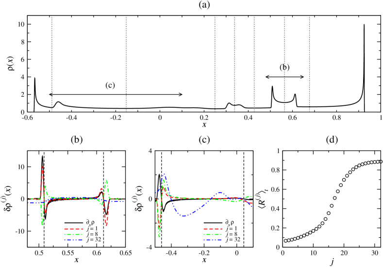
Figure 11: Snapshot of the distribution $\rho(x)$ (a) and CLVs $\delta\rho^{(j)}(x)$ (b,c) from the PF equation for globally-coupled noisy logistic maps (3) with $a=1.86$, $K=0.10$, and $\sigma=1\times 10^{-3}$. Vertical dotted lines in panel (a) show the partition of the support into the regions $S_{k}$, each containing one peak and bordered by local minima. In panels (b,c), black solid lines indicate the (arbitrarily scaled) first derivative of the distribution, the dashed lines show the CLVs $\delta\rho^{(j)}(x)$ with $j=1,8,32$ as stipulated in the legends, and the vertical dashed lines mark the positions of the peaks. Panel (d) shows the time-averaged residue $\langle R^{(j)}\rangle_{t}$ as a function of the index $j$ (see text).

We now turn our attention to the structure of the CLVs associated with these PF Lyapunov modes (Figure 11). Comparing the instantaneous distribution $\rho(x)$ (panel (a)) and CLVs $\delta\rho^{(j)}(x)$ (panels (b,c)), we find that the CLVs in the first region, i.e. those with small $j$, tend to be concentrated near the peaks in the distribution (red dashed lines and green dotted-dashed lines in panels (b,c)). Around each peak these CLVs are almost proportional to the first derivative of the distribution, $\rho^{\prime}(x)\equiv\partial_{x}\rho(x)$ (black solid line), but not globally, because the proportionality constant is different for each peak. This indicates that these modes shift peaks in the distribution at different amplitudes and directions, similarly to the positive collective mode found in the limit-cycle oscillators (Figure 5). In contrast, CLVs with large $j$ do not resemble such a patchwork of local first derivatives but tend to be distributed widely, both around the peaks and on top of the broad plateaux in between (blue double-dotted-dashed lines in Figure 11(b,c)). They therefore deform the plateau structures and/or change the weight balance between the peaks and the plateaux. To distinguish between these two types of Lyapunov modes, we quantify how similar each CLV $\delta\rho^{(j)}(x)$ is to the assembly of the local first derivatives, $\sum_{k}A_{k}^{(j)}\rho^{\prime}_{k}(x)$, where $k$ denotes the region $S_{k}=[x_{k},x_{k+1}]$ of the $k$th peak bordered at the local minima $x_{k}$ and $x_{k+1}$ of the distribution (dotted lines in Figure 11(a)) and $\rho^{\prime}_{k}(x)=\rho^{\prime}(x)$ if $x\in S_{k}$ and $0$ otherwise. Specifically, we compute the residue

$$R^{(j)}\equiv\sum_{k}\int_{S_{k}}\left[\delta\rho^{(j)}(x)-A_{k}^{(j)}\rho^{\prime}(x)\right]^{2}\mathrm{d}x$$ (8)

with the optimal choice of the coefficients, $A_{k}^{(j)}=\int_{S_{k}}\delta\rho^{(j)}(x)\rho^{\prime}(x)\mathrm{d}x/\int_{S_{k}}\rho^{\prime}(x)^{2}\mathrm{d}x$. This indeed shows a clear transition with varying $j$ (Figure 11(d)), which underpins the existence of the two regions in the Lyapunov spectrum. The same transition can also be seen in the spectrum of the IPRs, defined here by $Y_{2}^{(j)}=\langle\int\delta\rho^{(j)}(x)^{4}\mathrm{d}x\rangle_{t}$ with the normalization $\int\delta\rho^{(j)}(x)^{2}\mathrm{d}x=1$ (Figure 12(a)). Since the CLVs in the first region are localized around the density peaks, whose width is scaled by the noise amplitude $\sigma$, those IPRs take similar values when multiplied by $\sigma$ (Figure 12(b)). By contrast, IPRs in the second region decrease exponentially with increasing index $j$, setting a clear threshold index $j_{\rm th}$ for each noise amplitude $\sigma$ (intersection of two linear fits in Figure 12(b)). The threshold index $j_{\rm th}$ is found to increase logarithmically with decreasing $\sigma$ (Figure 12(c)), like $D_{\rm KY}$ and $j_{\rm inf}$ shown in the inset of Figure 10(a).

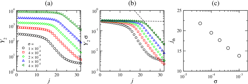
Figure 12: $Y_{2}^{(j)}$ spectrum of the PF Lyapunov modes for globally-coupled noisy logistic maps (3) with $a=1.86$ and $K=0.10$. (a) Spectra of the IPRs $Y_{2}^{(j)}$ for different noise amplitudes $\sigma$. (b) Same data are multiplied by $\sigma$. The dashed lines show linear fits (in the semilog scale) to the two spectrum regions for $\sigma=4\times 10^{-5}$ (top symbols), whose intersection determines the threshold index $j_{\rm th}(\sigma)$. (c) Threshold index $j_{\rm th}$ as a function of the noise amplitude $\sigma$.

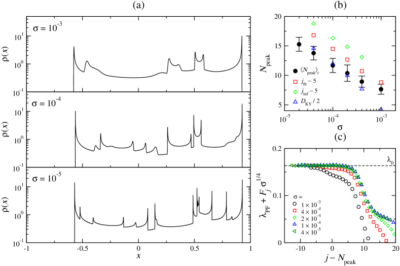
Figure 13: Number of density peaks and rescaling of the PF Lyapunov spectra for globally-coupled noisy logistic maps (3) with $a=1.86$ and $K=0.10$. (a) Typical instantaneous distributions $\rho(x)$ for different noise amplitudes $\sigma$. (b) Time-averaged number of peaks $N_{\rm peak}$ as a function of $\sigma$ (black solid circles). The bars indicate the standard deviation of the instantaneous values of $N_{\rm peak}$. The threshold index $j_{\rm th}$, the index of the inflection point $j_{\rm inf}$ and the Kaplan-Yorke dimension $D_{\rm KY}$ are also shown with shifts and factors stipulated in the legend. (c) PF Lyapunov spectra in the rescaled axes, exhibiting the asymptotic spectrum in the noiseless limit (same data and symbols as in Figure 10(a)). The horizontal dashed line indicates our estimate of the asymptotic LE, $\lambda_{0}=0.163(1)$.

The role played by the Lyapunov modes in the first region against the density peaks in the distribution suggests a direct connection between their numbers. Indeed, decreasing the noise amplitude $\sigma$, we find more and more peaks in the instantaneous distributions (Figure 13(a)), simply because the sharpest peak created from the superstable point becomes sharper and sharper. We then count the time-averaged number of peaks $N_{\rm peak}$ for each noise amplitude $\sigma$, and find that it varies logarithmically as $N_{\rm peak}\simeq N_{0}-C_{\rm peak}\log\sigma$ (black solid circles in Figure 13(b)), similarly to the number of the Lyapunov modes in the first region, or the threshold index, $j_{\rm th}\simeq j_{0}-C_{\rm th}\log\sigma$ (red squares; reproduced from Figure 12(c)). Moreover, the two coefficients are found to be very close, i.e., $C_{\rm peak}\approx C_{\rm th}$ (same slope in Figure 13(b)). This indicates that, for each peak added by decreasing the noise amplitude $\sigma$, a new Lyapunov mode is introduced to the first region of the PF spectrum, in order for this mode and the other existing ones to describe the instability of the newly added peak. The number of the peaks $N_{\rm peak}$ therefore controls the form of the Lyapunov spectrum in the first region: using $\lambda_{\rm PF}^{(j)}\simeq\lambda_{0}-F_{j}\sigma^{1/4}$ reported in Figure 10(b,c), we find a reasonably good collapse of the PF Lyapunov spectra within the axes $\lambda_{\rm PF}^{(j)}+F_{j}\sigma^{1/4}$ vs $j-N_{\rm peak}$ for sufficiently small noise amplitudes (Figure 13(c)). In particular, the ordinates in this representation indicate the LE values in the noiseless limit $\sigma\to 0$, which are surprisingly flat at $\lambda_{0}=0.163(1)$ in the first region.

To sum up, using the CLVs and the controlled noise distribution, we arrive at the following conclusion reached by Shibata et al. [9] on a firm basis: the effective dimension $D$ of the non-trivial collective chaos is finite when noise is added to the system, but it increases logarithmically with decreasing noise amplitude, $D\sim-\log\sigma$, and in particular diverges in the noiseless limit. In other words, the collective chaos in the noiseless system has infinite dimensionality. We have shown that this logarithmic divergence is due to the increasing number of the leading Lyapunov modes in the PF description, which exert various translational shifts to the density peaks in the distribution of the dynamical units. Therefore, the effective dimension of the collective chaos can be estimated, at least in this regime, by the number of these peaks $N_{\rm peak}$ as demonstrated in Figure 13(a), which can also be measured from the microscopic simulations of the maps, in principle.

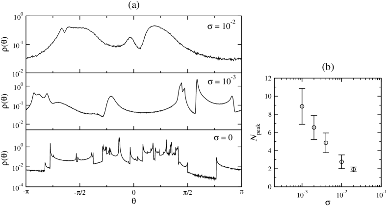
Figure 14: Instantaneous distributions (a) and number of peaks $N_{\rm peak}$ (b) for globally-coupled noisy limit-cycle oscillators (9) with various noise amplitudes $\sigma$. Configurations without folding are chosen for the instantaneous distributions shown in the panel (a), which are projected onto the angular coordinates $\theta_{i}\equiv\arg W_{i}$. The distribution for $\sigma=0$ is recaptured from Figure 1(b). For panel (b), symbols and bars indicate the mean and the standard deviation of the instantaneous numbers of the peaks. For both panels, the numbers of the oscillators are chosen between $10^{6}$ and $10^{8}$ to obtain reliable results.

On the basis of these results obtained for globally-coupled noisy logistic maps, we finally revisit the collective chaos studied in Section 2, exhibited by the globally-coupled limit-cycle oscillators. Given the similar structure of the instantaneous distributions (compare Figures 1(b) and 13(a)) and the similar role of the collective or PF Lyapunov modes (Figures 5(a,b) and 11), we expect that these two systems may share basic properties of the collective chaos. We therefore consider the limit-cycle oscillators in the presence of noise, added here sporadically for the sake of simplicity:

$$\dot{W}_{i}=W_{i}-(1+\mathrm{i}c_{2})|W_{i}|^{2}W_{i}+K(1+\mathrm{i}c_{1})(\langle W\rangle-W_{i})+\sum_{n\in\mathbb{Z}}\delta(t-n)\xi_{i}^{n},$$ (9)

where $\xi_{i}^{n}$ is drawn independently from the uniform distribution $[-\sigma,\sigma]$. We then measure the oscillator density projected on the angular coordinates $\theta_{i}\equiv\arg W_{i}$ for various noise amplitudes $\sigma$, and indeed find more peaks for lower values of $\sigma$ (Figure 14(a)). Counting the number of the peaks therein, averaged along the trajectory, we again identify a logarithmic increase $N_{\rm peak}\sim-\log\sigma$ (Figure 14(b)) like in the case of the logistic maps. Therefore, if we assume that there are roughly as many Lyapunov modes as the peaks for shifting them in this system too, the logarithmic growth in $N_{\rm peak}$ implies that the effective dimension of the collective chaos also increases and diverges in the noiseless limit. In this case, one should find more and more collective Lyapunov modes in addition to the ones found in Section 2 as increasing the system size further, though it is unattainable with the current machine power. Similarly, one can in principle study Lyapunov modes associated with the PF evolution for this system, but it seems to be unfeasible to track the evolution of the intricate, fractal-like density profile $\rho(W)$ in the complex plane (see Figure 1(c)) in a reliable manner with a finite number of bins. Although our results suggest that the logarithmic divergence takes place in $N_{\rm peak}$ as well as in the dimension of the collective chaos, all the more because peaks are formed and dispersed by stretching and folding of the support (and noise, if any) similarly to the logistic maps, providing a direct evidence for it, either numerically or theoretically, is a challenging open problem left for future studies.

5 Discussions and concluding remarks

In this paper, we have first shown that the standard Lyapunov analysis does capture the collective dynamics of large chaotic systems: it is encoded in a set of collective Lyapunov modes, which are delocalized over the collection of the dynamical units and thus exert relevant perturbations to macroscopic variables, without the need for finite-amplitude perturbations as opposed to some earlier claims [20, 21]. The CLVs allow us to detect such collective modes with the delocalization criterion, $Y_{2}^{(j)}\sim 1/N$, and to examine directly their role in the collective dynamics, as demonstrated for the regime of non-trivial collective chaos in globally-coupled limit-cycle oscillators (Section 2). Moreover, for globally-coupled systems, the instabilities of the collective dynamics can also be studied by the associated PF equation, whose Lyapunov modes, at least some of them, coincide with the collective modes of the original dynamical systems (Section 3). On the basis of this correspondence, in Section 4, we have analyzed in detail the non-trivial collective chaos in globally-coupled noisy logistic maps. We have then found leading PF Lyapunov modes, thus leading collective modes, assigned to translational shifts of dense clusters loosely formed by the dynamical units. The number of such clusters, $N_{\rm peak}$ increases logarithmically with decreasing noise amplitude $\sigma$, i.e., $N_{\rm peak}\sim-\log\sigma$, and so do the number of leading collective modes and other effective dimensions of collective chaos. This is expected to be a common feature of collective chaos that takes place on a bounded support undergoing stretching and folding, and indeed the logarithmic increase of $N_{\rm peak}$ was found also for globally-coupled noisy limit-cycle oscillators.

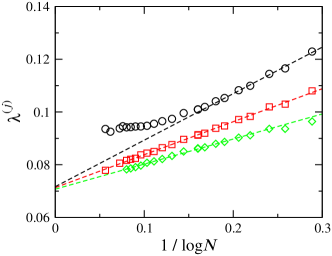
Figure 15: System-size dependence of the first three LEs for globally-coupled limit-cycle oscillators (2). The data shown in Figure 4(b) are plotted against $1/\log N$. The dashed lines show linear fits to the $1/\log N$ regime.

The existence of the collective modes, whether their number is finite or slowly increasing with system size, calls for revisiting the conventional definition of the extensivity of chaos in the presence of collective behavior, which assumes all the Lyapunov modes in the spectrum to be extensive. For globally-coupled systems, this form of extensivity does not hold even in the absence of collective behavior: in this case extensive LEs are sandwiched by “subextensive” bands composed of $\mathcal{O}(\log N)$ LEs at both ends of the spectrum, which vary logarithmically with system size as $\lambda\sim\lambda_{\infty}+\mathrm{const.}/\log N$ [23]. This picture is modified when collective behavior takes place (Figure 15): taking the first few LEs for the limit-cycle oscillators shown in Figure 4(b) and representing them as functions of $1/\log N$, we find that the second and subsequent LEs indeed obey the logarithmic size dependence for the subextensive exponents (dashed lines), while the first, collective mode (black circles) deviates from it as it develops the delocalized CLV structure with increasing system size. Moreover, as we have discussed in the previous section, there could exist more and more collective modes as the system size $N$ is further increased. Recalling the fact that the global field admits statistical fluctuations proportional to $1/\sqrt{N}$ around its time-evolving mean value [3], we might consider that each dynamical unit is subjected to an effective noise of amplitude $\sigma\sim 1/\sqrt{N}$ in this case. Then, our finding on the number of the density peaks implies that the number of the collective modes increases as $-\log\sigma\sim\log N$, adding another logarithmic subextensive band to the Lyapunov spectrum. A theoretical study is certainly needed to put this speculation on a firm basis. Seeking for a direct evidence of a collective mode in locally coupled systems is also an important issue left for future studies, in particular for the general understanding of the chaos extensivity.

Let us finally turn to the often-discussed but never-demonstrated analogy of NTCB to small dynamical systems. We have found for the limit-cycle oscillators that the collective LEs have the same set of the signs as what we would expect from the observed macroscopic dynamics, whether the number of positive collective LEs increases or not, and hence underpinned the analogy of NTCB to small dynamical systems. There is, however, an essential difference here: in contrast to small systems, the total number of the collective modes is not determined a priori. This implies that large dynamical systems may have far richer bifurcation structure at the macroscopic level, where collective exponents may not only change their signs but also be created and annihilated at the transition between two different NTCB regimes. It is important to clarify how this viewpoint is reconciled with some features like phase transitions, such as critical phenomena, reported by a few earlier studies [33, 34]. The collective Lyapunov modes should play central roles in tackling these fundamental issues left hitherto unexplored, which we believe deserve rather high computational cost needed for the investigations.

References

References

- [1] Chaté H and Manneville P 1992 Prog. Theor. Phys. 87 1–60
- [2] Kaneko K 1990 Phys. Rev. Lett. 65 1391–1394
- [3] Pikovsky A S and Kurths J 1994 Phys. Rev. Lett. 72 1644–1646
- [4] Kaneko K 1995 Physica D 86 158–170
- [5] Hakim V and Rappel W J 1992 Phys. Rev. A 46 R7347–R7350
- [6] Nakagawa N and Kuramoto Y 1993 Prog. Theor. Phys. 89 313–323
- [7] Nakagawa N and Kuramoto Y 1995 Physica D 80 307–316
- [8] Brunnet L, Chaté H and Manneville P 1994 Physica D 78 141–154
- [9] Shibata T, Chawanya T and Kaneko K 1999 Phys. Rev. Lett. 82 4424–4427
- [10] De Monte S, d’Ovidio F, Chaté H and Mosekilde E 2004 Phys. Rev. Lett. 92 254101
- [11] De Monte S, d’Ovidio F, Mosekilde E and Chaté H 2006 Prog. Theor. Phys. Suppl. 161 27–42
- [12] Bohr T, Grinstein G, He Y and Jayaprakash C 1987 Phys. Rev. Lett. 58 2155–2158
- [13] Eckmann J P and Ruelle D 1985 Rev. Mod. Phys. 57 617–656
- [14] Ruelle D 1982 Commun. Math. Phys. 87 287–302
- [15] Manneville P 1985 Liapounov exponents for the Kuramoto-Sivashinsky model (Lecture Notes in Physics vol 230) (Springer-Verlag Berlin Heidelberg New York Tokyo) pp 319–326
- [16] Keefe L 1989 Phys. Lett. A 140 317–322
- [17] Livi R, Politi A and Ruffo S 1986 J. Phys. A 19 2033–2040
- [18] O’Hern C S, Egolf D A and Greenside H S 1996 Phys. Rev. E 53 3374–3386
- [19] Egolf D A, Melnikov I V, Pesch W and Ecke R E 2000 Nature 404 733–736
- [20] Shibata T and Kaneko K 1998 Phys. Rev. Lett. 81 4116–4119
- [21] Cencini M, Falcioni M, Vergni D and Vulpiani A 1999 Physica D 130 58–72
- [22] Cencini M and Vulpiani A 2013 J. Phys. A 46 254019
- [23] Takeuchi K A, Chaté H, Ginelli F, Politi A and Torcini A 2011 Phys. Rev. Lett. 107 124101
- [24] Ginelli F, Poggi P, Turchi A, Chaté H, Livi R and Politi A 2007 Phys. Rev. Lett. 99 130601
- [25] Ginelli F, Chaté H, Livi R and Politi A 2013 J. Phys. A 46 254005
- [26] Takeuchi K A, Ginelli F and Chaté H 2009 Phys. Rev. Lett. 103 154103
- [27] Mirlin A D 2000 Phys. Rep. 326 259–382
- [28] Sano M and Sawada Y 1983 Phys. Lett. A 97 73–76
- [29] Jones M 2009 Stat. Methodol. 6 70–81
- [30] Teramae J n and Kuramoto Y 2001 Phys. Rev. E 63 036210
- [31] Yang H l, Takeuchi K A, Ginelli F, Chaté H and Radons G 2009 Phys. Rev. Lett. 102 074102
- [32] Takeuchi K A, Yang H l, Ginelli F, Radons G and Chaté H 2011 Phys. Rev. E 84 046214
- [33] Lemaître A and Chaté H 1999 Phys. Rev. Lett. 82 1140–1143
- [34] Marcq P, Chaté H and Manneville P 2006 Prog. Theor. Phys. Suppl. 161 244–250