Exact Cramer-Rao Bounds for Semi-blind Channel Estimation in Amplify-and-Forward Two-Way Relay Networks employing Square QAM Modulation

Saeed Abdallah and Ioannis N. Psaromiligkos The authors are with McGill University, Department of Electrical and Computer Engineering, 3480 University Street, Montreal, Quebec, H3A 2A7, Canada. Email: saeed.abdallah@mail.mcgill.ca; yannis@ece.mcgill.ca, phone: +1 (514) 398-2465, fax: +1 (514) 398-4470.*Corresponding author.
Abstract

In this paper, we derive the exact Cramer-Rao bounds (CRBs) for semi-blind channel estimation in amplify-and-forward two-way relay networks employing square QAM modulation. The derived bounds are used to show that the semi-blind approach, which exploits both the transmitted pilots and transmitted data symbols, can provide substantial improvements in estimation accuracy over the training-based approach which only uses pilot symbols to estimate the channel parameters. We also derive the more tractable modified CRB which accurately approximates the exact CRB at high SNR for low modulation orders.

Index Terms: Amplify and Forward, Cramer-Rao bound, Semi-blind Channel Estimation, Square QAM Modulation, Two-way Relays.

I Introduction

Amplify-and-forward (AF) two-way relay networks (TWRNs) [1] have recently received a lot of attention as a spectrally efficient approach for bidirectional communication between two terminals. In previous works on TWRNs, it is often assumed that the channel parameters are perfectly known at the terminals. In reality, however, these parameters have to be estimated, and an estimation error is always incurred. Since part of the channel information is required for self-interference cancellation at each terminal, the presence of estimation error means that self-interference cannot be completely cancelled, and the residual interference reduces the overall performance of the system.

The problem of estimating the channel in AF TWRNs has been addressed in a number of recent works [2, 3, 4, 5, 6, 7, 8, 9]. Most of these works adopt the pilot-based approach to channel estimation (c.f. [2]), which imposes an additional burden on the system and reduces the overall spectral efficiency. It is therefore important to investigate the application of semi-blind channel estimation which mitigates this burden by exploiting both pilots and the transmitted data to estimate the channel, or blind channel estimation which completely avoids this burden by relying only on the transmitted data for channel estimation. Researchers have recently started investigating such approaches [7, 8] in order to obtain better tradeoffs between estimation accuracy and spectral efficiency than the pilot-based approach. In [7], a semi-blind approach which jointly estimates the channel and detects the transmitted data for MIMO-OFDM TWRNs was developed using the expectation conditional maximization (ECM) algorithm. In [8], a blind channel estimation algorithm was proposed for TWRNs employing constant modulus (CM) signalling in the form of M𝑀MPSK modulation.

In order to evaluate the potential of semi-blind and blind approaches in the AF TWRN context and to provide a benchmark on the performance of such algorithms, it is very useful to know the Cramer-Rao bound (CRB) on achievable estimation accuracy. This bound is more easily obtained for the pilot-based approach, as has been done in [2]. However, for semi-blind and blind approaches, the task of deriving the CRB is more challenging because of the complicated form of the likelihood function when the statistics of the data symbols are taken into account. In [8] and [9], the derivation of the blind CRB for the case of CM signalling was simplified by ignoring the statistics of the data symbols and instead treating them as deterministic unknowns. To the best of our knowledge, however, the exact CRBs that take into account the statistics of the data have not been derived before for AF TWRNs. In this work, we fill this gap and we derive the exact CRBs for semi-blind channel estimation in AF TWRNs employing square QAM modulation. Due to its bandwidth efficiency, this class of modulation schemes is very important for today’s high datarate applications. The derived bounds also cover the blind and the pilot-based scenarios as special cases. We use the derived bounds to explore the potential of the semi-blind and blind approaches and show that substantial performance gains over the pilot-based approach can be achieved.

The rest of the paper is organized as follows. In Section II we present the system model. Our derivation of the CRB is presented in Section III. Simulation results are presented in IV. Finally, our conclusions are in Section V.
Refer to caption
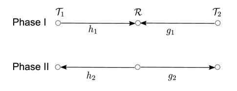
Figure 1: The two-way relay network with two source terminals and one relay node.

II System Model

We consider the half-duplex TWRN with two source nodes, 𝒯1subscript𝒯1\mathcal{T}_{1} and 𝒯2subscript𝒯2\mathcal{T}_{2}, and a single relaying node \mathcal{R}, shown in Fig. 1. The network operates in quasi-static flat-fading channel conditions. Each transmission period is divided into two phases. In the first phase, 𝒯1subscript𝒯1\mathcal{T}_{1} and 𝒯2subscript𝒯2\mathcal{T}_{2} simultaneously transmit to \mathcal{R}, and in the second phase \mathcal{R} broadcasts an amplified version of the received signal to both terminals. The semi-blind approach employs both pilot symbols and data symbols to estimate the channel parameters. More specifically, prior to transmitting data symbols, each terminal transmits a block of L𝐿L pilot symbols. We denote by 𝒕1[t11,,t1L]Tsubscript𝒕1superscriptsubscript𝑡11subscript𝑡1𝐿𝑇{\boldsymbol{t}}_{1}\triangleq[t_{11},\ldots,t_{1L}]^{T} and 𝒕2[t21,,t2L]subscript𝒕2subscript𝑡21subscript𝑡2𝐿{\boldsymbol{t}}_{2}\triangleq[t_{21},\ldots,t_{2L}] the vectors containing the pilot symbols transmitted by 𝒯1subscript𝒯1\mathcal{T}_{1} and 𝒯2subscript𝒯2\mathcal{T}_{2}, respectively. The received signal vector at \mathcal{R} during the training period is 𝒓t=h1𝒕1+g1𝒕2+𝝎subscript𝒓𝑡subscript1subscript𝒕1subscript𝑔1subscript𝒕2𝝎{\boldsymbol{r}}_{t}=h_{1}{\boldsymbol{t}}_{1}+g_{1}{\boldsymbol{t}}_{2}+{\boldsymbol{\omega}}, where h1subscript1h_{1} and g1subscript𝑔1g_{1} are the complex coefficients of the flat-fading channels 𝒯1subscript𝒯1\mathcal{T}_{1}\rightarrow\mathcal{R} and 𝒯2subscript𝒯2\mathcal{T}_{2}\rightarrow\mathcal{R}, respectively, and 𝝎𝝎{\boldsymbol{\omega}} is the circular complex white Gaussian noise with mean zero and covariance σ2𝑰superscript𝜎2𝑰\sigma^{2}{\boldsymbol{I}} (((denoted as 𝒞𝒞𝒩(0,σ2𝑰))\mathcal{CCN}(0,\sigma^{2}{\boldsymbol{I}})). The relay broadcasts A𝒓t𝐴subscript𝒓𝑡A{\boldsymbol{r}}_{t}, where A>0𝐴0A>0 is the amplification factor. The corresponding received signal vector at terminal 𝒯1subscript𝒯1\mathcal{T}_{1} is

𝒛t=Ah1h2𝒕1+Ag1h2𝒕2+Ah2𝝎+𝝎1subscript𝒛𝑡𝐴subscript1subscript2subscript𝒕1𝐴subscript𝑔1subscript2subscript𝒕2𝐴subscript2𝝎subscript𝝎1{\boldsymbol{z}}_{t}=Ah_{1}h_{2}{\boldsymbol{t}}_{1}+Ag_{1}h_{2}{\boldsymbol{t}}_{2}+Ah_{2}{\boldsymbol{\omega}}+{\boldsymbol{\omega}}_{1} (1)

where 𝝎1subscript𝝎1{\boldsymbol{\omega}}_{1} is also 𝒞𝒞𝒩(0,σ2𝑰)𝒞𝒞𝒩0superscript𝜎2𝑰\mathcal{CCN}(0,\sigma^{2}{\boldsymbol{I}}).

After transmitting the L𝐿L pilots, 𝒯1subscript𝒯1\mathcal{T}_{1} and 𝒯2subscript𝒯2\mathcal{T}_{2} transmit N𝑁N data symbols each. We denote by 𝒔1[s11,,s1N]Tsubscript𝒔1superscriptsubscript𝑠11subscript𝑠1𝑁𝑇{\boldsymbol{s}}_{1}\triangleq[s_{11},\ldots,s_{1N}]^{T} and 𝒔2[s21,,s2N]Tsubscript𝒔2superscriptsubscript𝑠21subscript𝑠2𝑁𝑇{\boldsymbol{s}}_{2}\triangleq[s_{21},\ldots,s_{2N}]^{T} the transmitted data symbol vectors of 𝒯1subscript𝒯1\mathcal{T}_{1} and 𝒯2subscript𝒯2\mathcal{T}_{2}, respectively. The received signal vector at \mathcal{R} is 𝒓=h1𝒔1+g1𝒔2+𝒏𝒓subscript1subscript𝒔1subscript𝑔1subscript𝒔2𝒏{\boldsymbol{r}}=h_{1}{\boldsymbol{s}}_{1}+g_{1}{\boldsymbol{s}}_{2}+{\boldsymbol{n}}, and the corresponding received signal vector at 𝒯1subscript𝒯1\mathcal{T}_{1} is

𝒛=Ah1h2𝒔1+Ag1h2𝒔2+Ah2𝒏+𝒏1𝒛𝐴subscript1subscript2subscript𝒔1𝐴subscript𝑔1subscript2subscript𝒔2𝐴subscript2𝒏subscript𝒏1{\boldsymbol{z}}=Ah_{1}h_{2}{\boldsymbol{s}}_{1}+Ag_{1}h_{2}{\boldsymbol{s}}_{2}+Ah_{2}{\boldsymbol{n}}+{\boldsymbol{n}}_{1} (2)

where 𝒏𝒏{\boldsymbol{n}} and 𝒏1subscript𝒏1{\boldsymbol{n}}_{1} are 𝒞𝒞𝒩(0,σ2𝑰)𝒞𝒞𝒩0superscript𝜎2𝑰\mathcal{CCN}(0,\sigma^{2}{\boldsymbol{I}}). The complex channel coefficients h1subscript1h_{1}, h2subscript2h_{2}, g1subscript𝑔1g_{1} and g2subscript𝑔2g_{2} are assumed to remain fixed during the transmission of the L𝐿L pilot symbols and N𝑁N data symbols.

We assume that both terminals employ square QAM modulation with possibly different modulation orders and transmission powers. Without loss of generality, we focus on the derivation of the CRB for channel estimation at terminal 𝒯1subscript𝒯1\mathcal{T}_{1}. For square QAM modulation, the total number of constellation points is M=22p𝑀superscript22𝑝M=2^{2p}, where p=1,2,3,𝑝123p=1,2,3,\ldots. Denoting by d𝑑d the intersymbol distance and letting dpd2subscript𝑑𝑝𝑑2d_{p}\triangleq\frac{d}{2}, the set of constellation points used by 𝒯2subscript𝒯2\mathcal{T}_{2} is given by S={±dp(2i1)±ȷdp(21)},i,=1,,2p1formulae-sequence𝑆plus-or-minusplus-or-minussubscript𝑑𝑝2𝑖1italic-ȷsubscript𝑑𝑝21𝑖1superscript2𝑝1S=\{\pm d_{p}(2i-1)\pm\jmath d_{p}(2\ell-1)\},i,\ell=1,\ldots,2^{p-1} [10]. The average transmitted power at 𝒯2subscript𝒯2\mathcal{T}_{2} is P2=𝔼{|s2k|2}=M16d2subscript𝑃2𝔼superscriptsubscript𝑠2𝑘2𝑀16superscript𝑑2P_{2}=\mathbb{E}\left\{|s_{2k}|^{2}\right\}=\frac{M-1}{6}d^{2}. We also let P1subscript𝑃1P_{1} be the avarage transmitted power at 𝒯1subscript𝒯1\mathcal{T}_{1}. Furthermore, we assume that the noise variance σ2superscript𝜎2\sigma^{2} is known at 𝒯1subscript𝒯1\mathcal{T}_{1}. In our work, we are interested in deriving the CRBs for the estimation of the composite channel parameters ah1h2𝑎subscript1subscript2a\triangleq h_{1}h_{2} and bg1h2𝑏subscript𝑔1subscript2b\triangleq g_{1}h_{2}, which are sufficient for data detection.

III Cramer-Rao Bounds

In this section, we derive the CRBs for the estimation of a𝑎a and b𝑏b. In addition to deriving the exact CRB, we will also consider the modified CRB (MCRB) [11] which is commonly used in the presence of random nuisance parameters and is more tractable than the exact CRB. In deriving these bounds, we also take into account the parameter |h2|2superscriptsubscript22|h_{2}|^{2} which, though not required for detection, appears in the likelihood function and thus affects the estimation performance. The unknowns parameters are thus a𝑎a, b𝑏b and |h2|2superscriptsubscript22|h_{2}|^{2} and are collected into the real vector 𝜽[{a},{a},{b},{b},|h2|2]T𝜽superscript𝑎𝑎𝑏𝑏superscriptsubscript22𝑇{\boldsymbol{\theta}}\triangleq[\Re\{a\},\Im\{a\},\Re\{b\},\Im\{b\},|h_{2}|^{2}]^{T}.

III-A Exact Cramer-Rao Bound

To derive the exact CRB for semi-blind channel estimation, we consider the joint likelihood of 𝒛tsubscript𝒛𝑡{\boldsymbol{z}}_{t} and 𝒛𝒛{\boldsymbol{z}}. Let 𝒛~[𝒛tT,𝒛T]T~𝒛superscriptsuperscriptsubscript𝒛𝑡𝑇superscript𝒛𝑇𝑇\tilde{{\boldsymbol{z}}}\triangleq[{\boldsymbol{z}}_{t}^{T},{\boldsymbol{z}}^{T}]^{T}, the joint likelihood is given by

f(𝒛~;𝜽)=1(πσ2(A2|h2|2+1))N+Le𝒛tAa𝒕1Ab𝒕22σ2(A2|h2|2+1)×k=1N1M(s2Se|zkAas1kAbs2|2σ2(A2|h2|2+1)).𝑓~𝒛𝜽1superscript𝜋superscript𝜎2superscript𝐴2superscriptsubscript221𝑁𝐿superscript𝑒superscriptnormsubscript𝒛𝑡𝐴𝑎subscript𝒕1𝐴𝑏subscript𝒕22superscript𝜎2superscript𝐴2superscriptsubscript221superscriptsubscriptproduct𝑘1𝑁1𝑀subscriptsubscript𝑠2𝑆superscript𝑒superscriptsubscript𝑧𝑘𝐴𝑎subscript𝑠1𝑘𝐴𝑏subscript𝑠22superscript𝜎2superscript𝐴2superscriptsubscript221\begin{split}f(\tilde{{\boldsymbol{z}}};{\boldsymbol{\theta}})&=\frac{1}{(\pi\sigma^{2}(A^{2}|h_{2}|^{2}+1))^{N+L}}e^{-\frac{\|{\boldsymbol{z}}_{t}-Aa{\boldsymbol{t}}_{1}-Ab{\boldsymbol{t}}_{2}\|^{2}}{\sigma^{2}(A^{2}|h_{2}|^{2}+1)}}\\ &\hskip 30.1388pt\times\prod_{k=1}^{N}\frac{1}{M}\bigg{(}\sum\limits_{s_{2}\in S}e^{-\frac{|z_{k}-Aas_{1k}-Abs_{2}|^{2}}{\sigma^{2}(A^{2}|h_{2}|^{2}+1)}}\bigg{)}.\end{split} (3)

The corresponding log-likelihood function is

(𝒛~;𝜽)=(N+L)log(πC)1C𝒛pAa𝒕1Ab𝒕22NlogM+k=1Nlog(s2Se1C|zkAas1kAbs2|2).~𝒛𝜽𝑁𝐿𝜋𝐶1𝐶superscriptdelimited-∥∥subscript𝒛𝑝𝐴𝑎subscript𝒕1𝐴𝑏subscript𝒕22𝑁𝑀superscriptsubscript𝑘1𝑁subscriptsubscript𝑠2𝑆superscript𝑒1𝐶superscriptsubscript𝑧𝑘𝐴𝑎subscript𝑠1𝑘𝐴𝑏subscript𝑠22\begin{split}&\mathcal{L}(\tilde{{\boldsymbol{z}}};{\boldsymbol{\theta}})=-(N+L)\log(\pi C)-\frac{1}{C}\|{\boldsymbol{z}}_{p}-Aa{\boldsymbol{t}}_{1}-Ab{\boldsymbol{t}}_{2}\|^{2}\\ &-N\log M+\sum\limits_{k=1}^{N}\log\bigg{(}\sum\limits_{s_{2}\in S}e^{-\frac{1}{C}|z_{k}-Aas_{1k}-Abs_{2}|^{2}}\bigg{)}.\end{split} (4)

where Cσ2(A2|h2|2+1)𝐶superscript𝜎2superscript𝐴2superscriptsubscript221C\triangleq\sigma^{2}(A^{2}|h_{2}|^{2}+1). Let 𝑰(θ)𝑰𝜃{\boldsymbol{I}}({\theta}) be the corresponding Fisher information matrix (FIM), and let Iθi,θjsubscript𝐼subscript𝜃𝑖subscript𝜃𝑗I_{\theta_{i},\theta_{j}} be the joint Fisher information between the parameters θisubscript𝜃𝑖\theta_{i} and θjsubscript𝜃𝑗\theta_{j}, where i,j=1,,5formulae-sequence𝑖𝑗15i,j=1,\ldots,5. Furthermore, to simplify our notation we let aR{a}subscript𝑎𝑅𝑎a_{R}\triangleq\Re\{a\}, aI{a}subscript𝑎𝐼𝑎a_{I}\triangleq\Im\{a\}, bR{b}subscript𝑏𝑅𝑏b_{R}\triangleq\Re\{b\}, bI{b}subscript𝑏𝐼𝑏b_{I}\triangleq\Im\{b\} and τ|h2|2𝜏superscriptsubscript22\tau\triangleq|h_{2}|^{2}. The matrix 𝑰(θ)𝑰𝜃{\boldsymbol{I}}({\theta}) is given by

𝑰(θ)=𝔼{2(𝒛~;𝜽)𝜽𝜽T}=[𝑰aa𝑰ab𝑰aτ𝑰abT𝑰bb𝑰bτ𝑰aτT𝑰bτTIτ,τ],𝑰𝜃𝔼superscript2~𝒛𝜽𝜽superscript𝜽𝑇matrixsubscript𝑰𝑎𝑎subscript𝑰𝑎𝑏subscript𝑰𝑎𝜏superscriptsubscript𝑰𝑎𝑏𝑇subscript𝑰𝑏𝑏subscript𝑰𝑏𝜏superscriptsubscript𝑰𝑎𝜏𝑇superscriptsubscript𝑰𝑏𝜏𝑇subscript𝐼𝜏𝜏\begin{split}{\boldsymbol{I}}({\theta})&=-\mathbb{E}\left\{\frac{\partial^{2}\mathcal{L}(\tilde{{\boldsymbol{z}}};{\boldsymbol{\theta}})}{\partial{\boldsymbol{\theta}}\partial{\boldsymbol{\theta}}^{T}}\right\}\\ &=\begin{bmatrix}{\boldsymbol{I}}_{aa}&{\boldsymbol{I}}_{ab}&{\boldsymbol{I}}_{a\tau}\\ {\boldsymbol{I}}_{ab}^{T}&{\boldsymbol{I}}_{bb}&{\boldsymbol{I}}_{b\tau}\\ {\boldsymbol{I}}_{a\tau}^{T}&{\boldsymbol{I}}_{b\tau}^{T}&I_{\tau,\tau}\end{bmatrix},\end{split} (5)

where

𝑰aa=[IaR,aRIaR,aIIaR,aIIaI,aI],𝑰ab=[IaR,bRIaR,bIIaI,bRIaI,bI],formulae-sequencesubscript𝑰𝑎𝑎matrixsubscript𝐼subscript𝑎𝑅subscript𝑎𝑅subscript𝐼subscript𝑎𝑅subscript𝑎𝐼subscript𝐼subscript𝑎𝑅subscript𝑎𝐼subscript𝐼subscript𝑎𝐼subscript𝑎𝐼subscript𝑰𝑎𝑏matrixsubscript𝐼subscript𝑎𝑅subscript𝑏𝑅subscript𝐼subscript𝑎𝑅subscript𝑏𝐼subscript𝐼subscript𝑎𝐼subscript𝑏𝑅subscript𝐼subscript𝑎𝐼subscript𝑏𝐼{\boldsymbol{I}}_{aa}=\begin{bmatrix}I_{a_{R},a_{R}}&I_{a_{R},a_{I}}\\ I_{a_{R},a_{I}}&I_{a_{I},a_{I}}\end{bmatrix},\ {\boldsymbol{I}}_{ab}=\begin{bmatrix}I_{a_{R},b_{R}}&I_{a_{R},b_{I}}\\ I_{a_{I},b_{R}}&I_{a_{I},b_{I}}\end{bmatrix}, (6)
𝑰bb=[IbR,bRIbR,bIIbR,bIIbI,bI],𝑰aτ=[IaR,τIaI,τ],𝑰bτ=[IbR,τIbI,τ].formulae-sequencesubscript𝑰𝑏𝑏matrixsubscript𝐼subscript𝑏𝑅subscript𝑏𝑅subscript𝐼subscript𝑏𝑅subscript𝑏𝐼subscript𝐼subscript𝑏𝑅subscript𝑏𝐼subscript𝐼subscript𝑏𝐼subscript𝑏𝐼formulae-sequencesubscript𝑰𝑎𝜏matrixsubscript𝐼subscript𝑎𝑅𝜏subscript𝐼subscript𝑎𝐼𝜏subscript𝑰𝑏𝜏matrixsubscript𝐼subscript𝑏𝑅𝜏subscript𝐼subscript𝑏𝐼𝜏{\boldsymbol{I}}_{bb}=\begin{bmatrix}I_{b_{R},b_{R}}&I_{b_{R},b_{I}}\\ I_{b_{R},b_{I}}&I_{b_{I},b_{I}}\end{bmatrix},\ {\boldsymbol{I}_{a\tau}}=\begin{bmatrix}I_{a_{R},\tau}\\ I_{a_{I},\tau}\end{bmatrix},\ {\boldsymbol{I}_{b\tau}}=\begin{bmatrix}I_{b_{R},\tau}\\ I_{b_{I},\tau}\end{bmatrix}. (7)

Before proceeding to obtain closed-form expressions for the elements of 𝑰(θ)𝑰𝜃{\boldsymbol{I}}(\theta), we will first factorize the likelihood function by taking into account the symmetric structure of square QAM modulation, following the approach proposed in [10]. This factorization will make it feasible to derive analytical expressions for the elements of 𝑰(θ)𝑰𝜃{\boldsymbol{I}}(\theta). We begin by rewriting the likelihood function in (3) as

f(𝒛~;𝜽)=1(πC)N+LMNe1C𝒛pAa𝒕1Ab𝒕22×k=1N(e1C|zkAas1k|2s2SeA2C|b|2|s2|2+2AC{(zkAas1k)bs2}).𝑓~𝒛𝜽1superscript𝜋𝐶𝑁𝐿superscript𝑀𝑁superscript𝑒1𝐶superscriptnormsubscript𝒛𝑝𝐴𝑎subscript𝒕1𝐴𝑏subscript𝒕22superscriptsubscriptproduct𝑘1𝑁superscript𝑒1𝐶superscriptsubscript𝑧𝑘𝐴𝑎subscript𝑠1𝑘2subscriptsubscript𝑠2𝑆superscript𝑒superscript𝐴2𝐶superscript𝑏2superscriptsubscript𝑠222𝐴𝐶superscriptsubscript𝑧𝑘𝐴𝑎subscript𝑠1𝑘𝑏subscript𝑠2\begin{split}&f(\tilde{{\boldsymbol{z}}};{\boldsymbol{\theta}})=\frac{1}{(\pi C)^{N+L}M^{N}}e^{-\frac{1}{C}\|{\boldsymbol{z}}_{p}-Aa{\boldsymbol{t}}_{1}-Ab{\boldsymbol{t}}_{2}\|^{2}}\times\\ &\prod_{k=1}^{N}\bigg{(}e^{-\frac{1}{C}|z_{k}-Aas_{1k}|^{2}}\sum\limits_{s_{2}\in S}e^{-\frac{A^{2}}{C}|b|^{2}|s_{2}|^{2}+\frac{2A}{C}\Re\{(z_{k}-Aas_{1k})^{*}bs_{2}\}}\bigg{)}.\end{split} (8)

Now, we let

Dk(𝜽)s2Se1CA2|b|2|s2|2+2AC{(zkAas1k)bs2}.subscript𝐷𝑘𝜽subscriptsubscript𝑠2𝑆superscript𝑒1𝐶superscript𝐴2superscript𝑏2superscriptsubscript𝑠222𝐴𝐶superscriptsubscript𝑧𝑘𝐴𝑎subscript𝑠1𝑘𝑏subscript𝑠2D_{k}({\boldsymbol{\theta}})\triangleq\sum\limits_{s_{2}\in S}e^{-\frac{1}{C}A^{2}|b|^{2}|s_{2}|^{2}+\frac{2A}{C}\Re\{(z_{k}-Aas_{1k})^{*}bs_{2}\}}. (9)

The inherent symmetry of the constellation set allows us to write (9) as a sum over the symbols in the first quadrant. If Q1subscript𝑄1Q_{1} is the set of constellation symbols that lie in the first quadrant, S𝑆S can be partitioned as S=Q1(Q1)Q1(Q1)𝑆subscript𝑄1subscript𝑄1superscriptsubscript𝑄1superscriptsubscript𝑄1S=Q_{1}\cup(-Q_{1})\cup Q_{1}^{*}\cup(-Q_{1}^{*}). Hence, we may rewrite Dk(𝜽)subscript𝐷𝑘𝜽D_{k}({\boldsymbol{\theta}}) as:

Dk(𝜽)=s2Q1e1CA2|b|2|s2|2(e2AC{(zkAas1k)bs2}+e2AC{(zkAas1k)bs2}+e2AC{(zkAas1k)bs2}+e2AC{(zkAas1k)bs2}).subscript𝐷𝑘𝜽subscriptsubscript𝑠2subscript𝑄1superscript𝑒1𝐶superscript𝐴2superscript𝑏2superscriptsubscript𝑠22superscript𝑒2𝐴𝐶superscriptsubscript𝑧𝑘𝐴𝑎subscript𝑠1𝑘𝑏subscript𝑠2superscript𝑒2𝐴𝐶superscriptsubscript𝑧𝑘𝐴𝑎subscript𝑠1𝑘𝑏superscriptsubscript𝑠2superscript𝑒2𝐴𝐶superscriptsubscript𝑧𝑘𝐴𝑎subscript𝑠1𝑘𝑏subscript𝑠2superscript𝑒2𝐴𝐶superscriptsubscript𝑧𝑘𝐴𝑎subscript𝑠1𝑘𝑏superscriptsubscript𝑠2\begin{split}D_{k}({\boldsymbol{\theta}})=&\sum\limits_{s_{2}\in Q_{1}}e^{-\frac{1}{C}A^{2}|b|^{2}|s_{2}|^{2}}\bigg{(}e^{\frac{2A}{C}\Re\{(z_{k}-Aas_{1k})^{*}bs_{2}\}}\\ &+e^{\frac{2A}{C}\Re\{(z_{k}-Aas_{1k})^{*}bs_{2}^{*}\}}+e^{-\frac{2A}{C}\Re\{(z_{k}-Aas_{1k})^{*}bs_{2}\}}\\ &+e^{-\frac{2A}{C}\Re\{(z_{k}-Aas_{1k})^{*}bs_{2}^{*}\}}\bigg{)}.\end{split} (10)

Noting that {(zkAas1k)bs2}={(zkAas1k)b}{s2}{(zkAas1k)b}{s2}superscriptsubscript𝑧𝑘𝐴𝑎subscript𝑠1𝑘𝑏subscript𝑠2superscriptsubscript𝑧𝑘𝐴𝑎subscript𝑠1𝑘𝑏subscript𝑠2superscriptsubscript𝑧𝑘𝐴𝑎subscript𝑠1𝑘𝑏subscript𝑠2\Re\{(z_{k}-Aas_{1k})^{*}bs_{2}\}=\Re\{(z_{k}-Aas_{1k})^{*}b\}\Re\{s_{2}\}-\Im\{(z_{k}-Aas_{1k})^{*}b\}\Im\{s_{2}\}, we rewrite (10) as

Dk(𝜽)=4s2Q1e1CA2|b|2|s2|2×cosh[2AC{(zkAas1k)b}{s2}]×cosh[2AC{(zkAas1k)b}{s2}].subscript𝐷𝑘𝜽4subscriptsubscript𝑠2subscript𝑄1superscript𝑒1𝐶superscript𝐴2superscript𝑏2superscriptsubscript𝑠222𝐴𝐶superscriptsubscript𝑧𝑘𝐴𝑎subscript𝑠1𝑘𝑏subscript𝑠22𝐴𝐶superscriptsubscript𝑧𝑘𝐴𝑎subscript𝑠1𝑘𝑏subscript𝑠2\begin{split}D_{k}({\boldsymbol{\theta}})&=4\sum\limits_{s_{2}\in Q_{1}}e^{-\frac{1}{C}A^{2}|b|^{2}|s_{2}|^{2}}\\ &\times\cosh\left[\frac{2A}{C}\Re\{(z_{k}-Aas_{1k})^{*}b\}\Re\{s_{2}\}\right]\\ &\times\cosh\left[\frac{2A}{C}\Im\{(z_{k}-Aas_{1k})^{*}b\}\Im\{s_{2}\}\right].\end{split} (11)

Moreover, for s2Q1subscript𝑠2subscript𝑄1s_{2}\in Q_{1}, we have that {s2},{s2}{(2i1)dp},i=1,,2p1formulae-sequencesubscript𝑠2subscript𝑠22𝑖1subscript𝑑𝑝𝑖1superscript2𝑝1\Re\{s_{2}\},\Im\{s_{2}\}\in\{(2i-1)d_{p}\},\ i=1,\ldots,2^{p-1}. Hence, (11) becomes

Dk(𝜽)=4i=12p1=12p1e1CA2|b|2((2i1)2+(21)2)dp2×cosh[2AC(2i1)dp{(zkAas1k)b}]×cosh[2AC(21)dp{(zkAas1k)b}].subscript𝐷𝑘𝜽4superscriptsubscript𝑖1superscript2𝑝1superscriptsubscript1superscript2𝑝1superscript𝑒1𝐶superscript𝐴2superscript𝑏2superscript2𝑖12superscript212superscriptsubscript𝑑𝑝22𝐴𝐶2𝑖1subscript𝑑𝑝superscriptsubscript𝑧𝑘𝐴𝑎subscript𝑠1𝑘𝑏2𝐴𝐶21subscript𝑑𝑝superscriptsubscript𝑧𝑘𝐴𝑎subscript𝑠1𝑘𝑏\begin{split}D_{k}({\boldsymbol{\theta}})&=4\sum\limits_{i=1}^{2^{p-1}}\sum\limits_{\ell=1}^{2^{p-1}}e^{-\frac{1}{C}A^{2}|b|^{2}((2i-1)^{2}+(2\ell-1)^{2})d_{p}^{2}}\times\\ &\cosh\left[\frac{2A}{C}(2i-1)d_{p}\Re\{(z_{k}-Aas_{1k})^{*}b\}\right]\times\\ &\cosh\left[\frac{2A}{C}(2\ell-1)d_{p}\Im\{(z_{k}-Aas_{1k})^{*}b\}\right].\end{split} (12)

From (12), we can see that, similar to the case in [10], Dk(𝜽)subscript𝐷𝑘𝜽D_{k}({\boldsymbol{\theta}}) is the product of two terms, one depending on {(zkAas1k)b}superscriptsubscript𝑧𝑘𝐴𝑎subscript𝑠1𝑘𝑏\Re\{(z_{k}-Aas_{1k})^{*}b\} and the other depending on {(zkAas1k)b}superscriptsubscript𝑧𝑘𝐴𝑎subscript𝑠1𝑘𝑏\Im\{(z_{k}-Aas_{1k})^{*}b\}:

Dk(𝜽)=4Fθ(uk)Fθ(vk),subscript𝐷𝑘𝜽4subscript𝐹𝜃subscript𝑢𝑘subscript𝐹𝜃subscript𝑣𝑘D_{k}({\boldsymbol{\theta}})=4F_{\theta}(u_{k})F_{\theta}(v_{k}), (13)

where

Fθ(t)i=12p1e1CA2dp2|b|2(2i1)2cosh(2AdpC(2i1)t),subscript𝐹𝜃𝑡superscriptsubscript𝑖1superscript2𝑝1superscript𝑒1𝐶superscript𝐴2superscriptsubscript𝑑𝑝2superscript𝑏2superscript2𝑖122𝐴subscript𝑑𝑝𝐶2𝑖1𝑡F_{\theta}(t)\triangleq\sum\limits_{i=1}^{2^{p-1}}e^{-\frac{1}{C}A^{2}d_{p}^{2}|b|^{2}(2i-1)^{2}}\cosh\left(\frac{2Ad_{p}}{C}(2i-1)t\right), (14)
uk{(zkAas1k)b}={zkAas1k}bR+{zkAas1k}bIsubscript𝑢𝑘superscriptsubscript𝑧𝑘𝐴𝑎subscript𝑠1𝑘𝑏subscript𝑧𝑘𝐴𝑎subscript𝑠1𝑘subscript𝑏𝑅subscript𝑧𝑘𝐴𝑎subscript𝑠1𝑘subscript𝑏𝐼\begin{split}u_{k}&\triangleq\Re\{(z_{k}-Aas_{1k})^{*}b\}\\ &=\Re\{z_{k}-Aas_{1k}\}b_{R}+\Im\{z_{k}-Aas_{1k}\}b_{I}\end{split} (15)

and

vk{(zkAas1k)b}={zkAas1k}bI{zkAas1k}bR.subscript𝑣𝑘superscriptsubscript𝑧𝑘𝐴𝑎subscript𝑠1𝑘𝑏subscript𝑧𝑘𝐴𝑎subscript𝑠1𝑘subscript𝑏𝐼subscript𝑧𝑘𝐴𝑎subscript𝑠1𝑘subscript𝑏𝑅\begin{split}v_{k}&\triangleq\Im\{(z_{k}-Aas_{1k})^{*}b\}\\ &=\Re\{z_{k}-Aas_{1k}\}b_{I}-\Im\{z_{k}-Aas_{1k}\}b_{R}.\end{split} (16)

Before proceeding, we simplify our notation by letting βiAdpC(2i1)subscript𝛽𝑖𝐴subscript𝑑𝑝𝐶2𝑖1\beta_{i}\triangleq\frac{Ad_{p}}{C}(2i-1) and γiA2dp2C(2i1)2subscript𝛾𝑖superscript𝐴2superscriptsubscript𝑑𝑝2𝐶superscript2𝑖12\gamma_{i}\triangleq\frac{A^{2}d_{p}^{2}}{C}(2i-1)^{2} for i=1,,2p1𝑖1superscript2𝑝1i=1,\ldots,2^{p-1}. Using the newly defined βisubscript𝛽𝑖\beta_{i}, γisubscript𝛾𝑖\gamma_{i}, we can write Fθ(t)subscript𝐹𝜃𝑡F_{\theta}(t) as

Fθ(t)i=12p1eγi|b|2cosh(2βit).subscript𝐹𝜃𝑡superscriptsubscript𝑖1superscript2𝑝1superscript𝑒subscript𝛾𝑖superscript𝑏22subscript𝛽𝑖𝑡F_{\theta}(t)\triangleq\sum\limits_{i=1}^{2^{p-1}}e^{-\gamma_{i}|b|^{2}}\cosh\left(2\beta_{i}t\right). (17)

Using (13), the likelihood function becomes

f(𝒛~;θ)=1(πC)N+Le1C𝒛pAa𝒕1Ab𝒕22×k=1N1M(e1C|zkAas1k|24Fθ(uk)Fθ(vk)).𝑓~𝒛𝜃1superscript𝜋𝐶𝑁𝐿superscript𝑒1𝐶superscriptnormsubscript𝒛𝑝𝐴𝑎subscript𝒕1𝐴𝑏subscript𝒕22superscriptsubscriptproduct𝑘1𝑁1𝑀superscript𝑒1𝐶superscriptsubscript𝑧𝑘𝐴𝑎subscript𝑠1𝑘24subscript𝐹𝜃subscript𝑢𝑘subscript𝐹𝜃subscript𝑣𝑘\begin{split}f(\tilde{{\boldsymbol{z}}};\theta)&=\frac{1}{(\pi C)^{N+L}}e^{-\frac{1}{C}\|{\boldsymbol{z}}_{p}-Aa{\boldsymbol{t}}_{1}-Ab{\boldsymbol{t}}_{2}\|^{2}}\\ &\times\prod_{k=1}^{N}\frac{1}{M}\bigg{(}e^{-\frac{1}{C}|z_{k}-Aas_{1k}|^{2}}4F_{\theta}(u_{k})F_{\theta}(v_{k})\bigg{)}.\end{split} (18)

As we shall see shortly, the RVs uksubscript𝑢𝑘u_{k} and vksubscript𝑣𝑘v_{k} are independent, a fact which will simplify our derivation of the FIM. It is also useful to define two new RVs, xk{zkAas1k}subscript𝑥𝑘subscript𝑧𝑘𝐴𝑎subscript𝑠1𝑘x_{k}\triangleq\Re\{z_{k}-Aas_{1k}\} and yk{zkAas1k}subscript𝑦𝑘subscript𝑧𝑘𝐴𝑎subscript𝑠1𝑘y_{k}\triangleq\Im\{z_{k}-Aas_{1k}\}. The pairs {uk,vk}subscript𝑢𝑘subscript𝑣𝑘\{u_{k},v_{k}\} and pair {xk,yk}subscript𝑥𝑘subscript𝑦𝑘\{x_{k},y_{k}\} are related through the following linear transformation

[ukvk]=[bRbIbIbR][xkyk].matrixsubscript𝑢𝑘subscript𝑣𝑘matrixsubscript𝑏𝑅subscript𝑏𝐼subscript𝑏𝐼subscript𝑏𝑅matrixsubscript𝑥𝑘subscript𝑦𝑘\begin{bmatrix}u_{k}\\ v_{k}\end{bmatrix}=\begin{bmatrix}b_{R}&b_{I}\\ b_{I}&-b_{R}\end{bmatrix}\begin{bmatrix}x_{k}\\ y_{k}\end{bmatrix}. (19)

Both pairs of RVs will be used in deriving the elements of the 𝑰(θ)𝑰𝜃{\boldsymbol{I}}(\theta). It is easy to see that the joint PDF of xksubscript𝑥𝑘x_{k} and yksubscript𝑦𝑘y_{k} is

fX,Y(xk,yk)=4πMCexk2+yk2CFθ(bRxk+bIyk)Fθ(bIxkbRyk).subscript𝑓𝑋𝑌subscript𝑥𝑘subscript𝑦𝑘4𝜋𝑀𝐶superscript𝑒superscriptsubscript𝑥𝑘2superscriptsubscript𝑦𝑘2𝐶subscript𝐹𝜃subscript𝑏𝑅subscript𝑥𝑘subscript𝑏𝐼subscript𝑦𝑘subscript𝐹𝜃subscript𝑏𝐼subscript𝑥𝑘subscript𝑏𝑅subscript𝑦𝑘f_{X,Y}(x_{k},y_{k})=\frac{4}{\pi MC}e^{-\frac{x_{k}^{2}+y_{k}^{2}}{C}}F_{\theta}(b_{R}x_{k}+b_{I}y_{k})F_{\theta}(b_{I}x_{k}-b_{R}y_{k}). (20)

Using (19) and (20), we obtain the joint PDF of uksubscript𝑢𝑘u_{k} and vksubscript𝑣𝑘v_{k}:

fU,V(uk,vk)=4πMC|b|2euk2+vk2C|b|2Fθ(uk)Fθ(vk).subscript𝑓𝑈𝑉subscript𝑢𝑘subscript𝑣𝑘4𝜋𝑀𝐶superscript𝑏2superscript𝑒superscriptsubscript𝑢𝑘2superscriptsubscript𝑣𝑘2𝐶superscript𝑏2subscript𝐹𝜃subscript𝑢𝑘subscript𝐹𝜃subscript𝑣𝑘f_{U,V}(u_{k},v_{k})=\frac{4}{\pi MC|b|^{2}}e^{-\frac{u_{k}^{2}+v_{k}^{2}}{C|b|^{2}}}F_{\theta}(u_{k})F_{\theta}(v_{k}). (21)

It is clear from (21) that the RVs uksubscript𝑢𝑘u_{k} and vksubscript𝑣𝑘v_{k} are independent and identically distributed (i.i.d.) with respective PDFs

fU(uk)=2MπC|b|2euk2C|b|2Fθ(uk),subscript𝑓𝑈subscript𝑢𝑘2𝑀𝜋𝐶superscript𝑏2superscript𝑒superscriptsubscript𝑢𝑘2𝐶superscript𝑏2subscript𝐹𝜃subscript𝑢𝑘f_{U}(u_{k})=\frac{2}{\sqrt{M\pi C|b|^{2}}}e^{-\frac{u_{k}^{2}}{C|b|^{2}}}F_{\theta}(u_{k}), (22)

and

fV(vk)=2MπC|b|2evk2C|b|2Fθ(vk).subscript𝑓𝑉subscript𝑣𝑘2𝑀𝜋𝐶superscript𝑏2superscript𝑒superscriptsubscript𝑣𝑘2𝐶superscript𝑏2subscript𝐹𝜃subscript𝑣𝑘f_{V}(v_{k})=\frac{2}{\sqrt{M\pi C|b|^{2}}}e^{-\frac{v_{k}^{2}}{C|b|^{2}}}F_{\theta}(v_{k}). (23)

Going back to the log-likelihood function in (4), we may now rewrite it as

(𝒛~;𝜽)=(N+L)log(πC)1C𝒛pAa𝒕1Ab𝒕22+Nlog4M1C𝒛Aa𝒔12+k=1NlogFθ(uk)+k=1NlogFθ(vk).~𝒛𝜽𝑁𝐿𝜋𝐶1𝐶superscriptdelimited-∥∥subscript𝒛𝑝𝐴𝑎subscript𝒕1𝐴𝑏subscript𝒕22𝑁4𝑀1𝐶superscriptdelimited-∥∥𝒛𝐴𝑎subscript𝒔12superscriptsubscript𝑘1𝑁subscript𝐹𝜃subscript𝑢𝑘superscriptsubscript𝑘1𝑁subscript𝐹𝜃subscript𝑣𝑘\begin{split}\mathcal{L}(\tilde{{\boldsymbol{z}}};{\boldsymbol{\theta}})=&-(N+L)\log(\pi C)-\frac{1}{C}\|{\boldsymbol{z}}_{p}-Aa{\boldsymbol{t}}_{1}-Ab{\boldsymbol{t}}_{2}\|^{2}+\\ &N\log\frac{4}{M}-\frac{1}{C}\|{\boldsymbol{z}}-Aa{\boldsymbol{s}}_{1}\|^{2}+\\ &\sum\limits_{k=1}^{N}\log F_{\theta}(u_{k})+\sum\limits_{k=1}^{N}\log F_{\theta}(v_{k}).\end{split} (24)

From (24) we see that the main task in obtaining analytical expressions for the elements of 𝑰(θ)𝑰𝜃{\boldsymbol{I}}(\theta) is the evaluation of the expectations 𝔼{2logFθ(uk)θiθj}𝔼superscript2subscript𝐹𝜃subscript𝑢𝑘subscript𝜃𝑖subscript𝜃𝑗\mathbb{E}\left\{\frac{\partial^{2}\log F_{\theta}(u_{k})}{\partial\theta_{i}\partial\theta_{j}}\right\} and 𝔼{2logFθ(vk)θiθj}𝔼superscript2subscript𝐹𝜃subscript𝑣𝑘subscript𝜃𝑖subscript𝜃𝑗\mathbb{E}\left\{\frac{\partial^{2}\log F_{\theta}(v_{k})}{\partial\theta_{i}\partial\theta_{j}}\right\} for i,j=1,,5formulae-sequence𝑖𝑗15i,j=1,\ldots,5. Letting

Bk(ij)2Fθ(uk)θiθjFθ(uk),Gk(ij)Fθ(uk)θiFθ(uk)θjFθ(uk)2,formulae-sequencesuperscriptsubscript𝐵𝑘𝑖𝑗superscript2subscript𝐹𝜃subscript𝑢𝑘subscript𝜃𝑖subscript𝜃𝑗subscript𝐹𝜃subscript𝑢𝑘superscriptsubscript𝐺𝑘𝑖𝑗subscript𝐹𝜃subscript𝑢𝑘subscript𝜃𝑖subscript𝐹𝜃subscript𝑢𝑘subscript𝜃𝑗subscript𝐹𝜃superscriptsubscript𝑢𝑘2B_{k}^{(ij)}\triangleq\frac{\frac{\partial^{2}F_{\theta}(u_{k})}{\partial\theta_{i}\partial\theta_{j}}}{F_{\theta}(u_{k})},\ \ \ \ \ G_{k}^{(ij)}\triangleq\frac{\frac{\partial F_{\theta}(u_{k})}{\partial\theta_{i}}\frac{\partial F_{\theta}(u_{k})}{\partial\theta_{j}}}{F_{\theta}(u_{k})^{2}}, (25)

and

Hk(ij)2Fθ(vk)θiθjFθ(vk),Wk(ij)Fθ(vk)θiFθ(vk)θjFθ(vk)2,formulae-sequencesuperscriptsubscript𝐻𝑘𝑖𝑗superscript2subscript𝐹𝜃subscript𝑣𝑘subscript𝜃𝑖subscript𝜃𝑗subscript𝐹𝜃subscript𝑣𝑘superscriptsubscript𝑊𝑘𝑖𝑗subscript𝐹𝜃subscript𝑣𝑘subscript𝜃𝑖subscript𝐹𝜃subscript𝑣𝑘subscript𝜃𝑗subscript𝐹𝜃superscriptsubscript𝑣𝑘2H_{k}^{(ij)}\triangleq\frac{\frac{\partial^{2}F_{\theta}(v_{k})}{\partial\theta_{i}\partial\theta_{j}}}{F_{\theta}(v_{k})},\ \ \ \ \ W_{k}^{(ij)}\triangleq\frac{\frac{\partial F_{\theta}(v_{k})}{\partial\theta_{i}}\frac{\partial F_{\theta}(v_{k})}{\partial\theta_{j}}}{F_{\theta}(v_{k})^{2}}, (26)

we have that

2logFθ(uk)θiθj=Bk(ij)Gk(ij),superscript2subscript𝐹𝜃subscript𝑢𝑘subscript𝜃𝑖subscript𝜃𝑗superscriptsubscript𝐵𝑘𝑖𝑗superscriptsubscript𝐺𝑘𝑖𝑗\frac{\partial^{2}\log F_{\theta}(u_{k})}{\partial\theta_{i}\partial\theta_{j}}=B_{k}^{(ij)}-G_{k}^{(ij)}, (27)

and

2logFθ(vk)θiθj=Hk(ij)Wk(ij).superscript2subscript𝐹𝜃subscript𝑣𝑘subscript𝜃𝑖subscript𝜃𝑗superscriptsubscript𝐻𝑘𝑖𝑗superscriptsubscript𝑊𝑘𝑖𝑗\frac{\partial^{2}\log F_{\theta}(v_{k})}{\partial\theta_{i}\partial\theta_{j}}=H_{k}^{(ij)}-W_{k}^{(ij)}. (28)

Despite the factorization of the log-likelihood function, the derivation of analytical expressions for the elements of 𝑰(θ)𝑰𝜃{\boldsymbol{I}}({\theta}) requires tedious calculations. Due to space limitations, we will provide detailed derivations for only some of these elements. For the remaining elements we will provide only the resulting analytical expressions. We begin with the first diagonal element of the FIM, IaR,aRsubscript𝐼subscript𝑎𝑅subscript𝑎𝑅I_{a_{R},a_{R}}. We have

𝔼{2(𝒛~;𝜽)aR2}=2A2C𝒕1H𝒕12A2C𝒔1H𝒔1+k=1N𝔼{Bk(11)Gk(11)}+k=1N𝔼{Hk(11)Wk(11)}.𝔼superscript2~𝒛𝜽superscriptsubscript𝑎𝑅22superscript𝐴2𝐶superscriptsubscript𝒕1𝐻subscript𝒕12superscript𝐴2𝐶superscriptsubscript𝒔1𝐻subscript𝒔1superscriptsubscript𝑘1𝑁𝔼superscriptsubscript𝐵𝑘11superscriptsubscript𝐺𝑘11superscriptsubscript𝑘1𝑁𝔼superscriptsubscript𝐻𝑘11superscriptsubscript𝑊𝑘11\begin{split}&\mathbb{E}\left\{\frac{\partial^{2}\mathcal{L}(\tilde{{\boldsymbol{z}}};{\boldsymbol{\theta}})}{\partial a_{R}^{2}}\right\}=-\frac{2A^{2}}{C}{\boldsymbol{t}}_{1}^{H}{\boldsymbol{t}}_{1}-\frac{2A^{2}}{C}{\boldsymbol{s}}_{1}^{H}{\boldsymbol{s}}_{1}\\ &+\sum\limits_{k=1}^{N}\mathbb{E}\left\{B_{k}^{(11)}-G_{k}^{(11)}\right\}+\sum\limits_{k=1}^{N}\mathbb{E}\left\{H_{k}^{(11)}-W_{k}^{(11)}\right\}.\\ \end{split} (29)

We show in Appendix A that

𝔼{Bk(11)}=8A2Mi=12p1βi2{s1kb}2,\mathbb{E}\left\{B_{k}^{(11)}\right\}=\frac{8A^{2}}{\sqrt{M}}\sum\limits_{i=1}^{2^{p-1}}\beta_{i}^{2}\Re\{s_{1k}^{*}b\}^{2}, (30)

and

𝔼{Hk(11)}=8A2Mi=12p1βi2{s1kb}2.\mathbb{E}\left\{H_{k}^{(11)}\right\}=\frac{8A^{2}}{\sqrt{M}}\sum\limits_{i=1}^{2^{p-1}}\beta_{i}^{2}\Im\{s_{1k}^{*}b\}^{2}. (31)

To obtain 𝔼{Gk(11)}𝔼superscriptsubscript𝐺𝑘11\mathbb{E}\left\{G_{k}^{(11)}\right\}, we need the first derivative of Fθ(uk)subscript𝐹𝜃subscript𝑢𝑘F_{\theta}(u_{k}) with respect to aRsubscript𝑎𝑅a_{R}, which is given by

Fθ(uk)aR=2A{s1kb}i=12p1βieγi|b|2sinh[2βiuk].subscript𝐹𝜃subscript𝑢𝑘subscript𝑎𝑅2𝐴superscriptsubscript𝑠1𝑘𝑏superscriptsubscript𝑖1superscript2𝑝1subscript𝛽𝑖superscript𝑒subscript𝛾𝑖superscript𝑏22subscript𝛽𝑖subscript𝑢𝑘\begin{split}\frac{\partial F_{\theta}(u_{k})}{\partial a_{R}}=-2A\Re\{s_{1k}^{*}b\}\sum\limits_{i=1}^{2^{p-1}}\beta_{i}e^{-\gamma_{i}|b|^{2}}\sinh[2\beta_{i}u_{k}].\end{split} (32)

From (32), we see that we can evaluate 𝔼{Gk(11)}𝔼superscriptsubscript𝐺𝑘11\mathbb{E}\left\{G_{k}^{(11)}\right\} using the PDF fU(uk)subscript𝑓𝑈subscript𝑢𝑘f_{U}(u_{k}) in (22). We thus obtain

𝔼{Gk(11)}={s1kb}2Γ1,\mathbb{E}\left\{G_{k}^{(11)}\right\}=\Re\{s_{1k}^{*}b\}^{2}\Gamma_{1}, (33)

where

Γ1=8A2πMC|b|2f2(t)Fθ(t)et2C|b|2𝑑t,subscriptΓ18superscript𝐴2𝜋𝑀𝐶superscript𝑏2superscriptsubscriptsuperscript𝑓2𝑡subscript𝐹𝜃𝑡superscript𝑒superscript𝑡2𝐶superscript𝑏2differential-d𝑡\Gamma_{1}=\frac{8A^{2}}{\sqrt{\pi MC|b|^{2}}}\int_{-\infty}^{\infty}\frac{f^{2}(t)}{F_{\theta}(t)}e^{-\frac{t^{2}}{C|b|^{2}}}dt, (34)

and

f(t)=i=12p1βieγi|b|2sinh[2βit].𝑓𝑡superscriptsubscript𝑖1superscript2𝑝1subscript𝛽𝑖superscript𝑒subscript𝛾𝑖superscript𝑏22subscript𝛽𝑖𝑡f(t)=\sum\limits_{i=1}^{2^{p-1}}\beta_{i}e^{-\gamma_{i}|b|^{2}}\sinh[2\beta_{i}t]. (35)

Moreover, it can be easily verified that

𝔼{Wk(11)}={s1kb}2Γ1,\mathbb{E}\left\{W_{k}^{(11)}\right\}=\Im\{s_{1k}^{*}b\}^{2}\Gamma_{1}, (36)

Hence,

IaR,aR=2A2C𝒕1H𝒕1+2A2Ck=1N𝒔1H𝒔1|b|2𝒔1H𝒔1(8A2Mi=12p1βi2Γ1).subscript𝐼subscript𝑎𝑅subscript𝑎𝑅2superscript𝐴2𝐶superscriptsubscript𝒕1𝐻subscript𝒕12superscript𝐴2𝐶superscriptsubscript𝑘1𝑁superscriptsubscript𝒔1𝐻subscript𝒔1superscript𝑏2superscriptsubscript𝒔1𝐻subscript𝒔18superscript𝐴2𝑀superscriptsubscript𝑖1superscript2𝑝1superscriptsubscript𝛽𝑖2subscriptΓ1\begin{split}&I_{a_{R},a_{R}}=\frac{2A^{2}}{C}{\boldsymbol{t}}_{1}^{H}{\boldsymbol{t}}_{1}+\frac{2A^{2}}{C}\sum\limits_{k=1}^{N}{\boldsymbol{s}}_{1}^{H}{\boldsymbol{s}}_{1}\\ &-|b|^{2}{\boldsymbol{s}}_{1}^{H}{\boldsymbol{s}}_{1}\left(\frac{8A^{2}}{\sqrt{M}}\sum\limits_{i=1}^{2^{p-1}}\beta_{i}^{2}-\Gamma_{1}\right).\end{split} (37)

Regarding the second diagonal element of 𝑰(θ)𝑰𝜃{\boldsymbol{I}}(\theta), it can be easily shown that IaI,aI=IaR,aRsubscript𝐼subscript𝑎𝐼subscript𝑎𝐼subscript𝐼subscript𝑎𝑅subscript𝑎𝑅I_{a_{I},a_{I}}=I_{a_{R},a_{R}}.

For the third diagonal element of 𝑰(θ)𝑰𝜃{\boldsymbol{I}}(\theta), we have

𝔼{2(𝒛~;𝜽)bR2}=2A2C𝒕2H𝒕2+k=1N𝔼{Bk(33)Gk(33)}+k=1N𝔼{Hk(33)Wk(33)}.𝔼superscript2~𝒛𝜽superscriptsubscript𝑏𝑅22superscript𝐴2𝐶superscriptsubscript𝒕2𝐻subscript𝒕2superscriptsubscript𝑘1𝑁𝔼superscriptsubscript𝐵𝑘33superscriptsubscript𝐺𝑘33superscriptsubscript𝑘1𝑁𝔼superscriptsubscript𝐻𝑘33superscriptsubscript𝑊𝑘33\begin{split}\mathbb{E}\left\{\frac{\partial^{2}\mathcal{L}(\tilde{{\boldsymbol{z}}};{\boldsymbol{\theta}})}{\partial b_{R}^{2}}\right\}&=-\frac{2A^{2}}{C}{\boldsymbol{t}}_{2}^{H}{\boldsymbol{t}}_{2}+\sum\limits_{k=1}^{N}\mathbb{E}\left\{B_{k}^{(33)}-G_{k}^{(33)}\right\}\\ &+\sum\limits_{k=1}^{N}\mathbb{E}\left\{H_{k}^{(33)}-W_{k}^{(33)}\right\}.\end{split} (38)

Furthermore, we show in Appendix B that

𝔼{Bk(33)}=𝔼{Hk(33)}=16Mi=12p1=12p1γiγbI2.𝔼superscriptsubscript𝐵𝑘33𝔼superscriptsubscript𝐻𝑘3316𝑀superscriptsubscript𝑖1superscript2𝑝1superscriptsubscript1superscript2𝑝1subscript𝛾𝑖subscript𝛾superscriptsubscript𝑏𝐼2\begin{split}\mathbb{E}\left\{B_{k}^{(33)}\right\}=\mathbb{E}\left\{H_{k}^{(33)}\right\}=\frac{16}{M}\sum\limits_{i=1}^{2^{p-1}}\sum\limits_{\ell=1}^{2^{p-1}}\gamma_{i}\gamma_{\ell}b_{I}^{2}.\end{split} (39)

To find 𝔼{Gk(33)}𝔼superscriptsubscript𝐺𝑘33\mathbb{E}\left\{G_{k}^{(33)}\right\}, we obtain the derivative of Fθ(uk)subscript𝐹𝜃subscript𝑢𝑘F_{\theta}(u_{k}) with respect to bRsubscript𝑏𝑅b_{R}, which is given by

q1(xk,yk)Fθ(bRxk+bIyk)bR=i=12p12γibReγi|b|2cosh[2βi(bRxk+bIyk)]+i=12p12βixkeγi|b|2sinh[2βi(bRxk+bIyk)].subscript𝑞1subscript𝑥𝑘subscript𝑦𝑘subscript𝐹𝜃subscript𝑏𝑅subscript𝑥𝑘subscript𝑏𝐼subscript𝑦𝑘subscript𝑏𝑅superscriptsubscript𝑖1superscript2𝑝12subscript𝛾𝑖subscript𝑏𝑅superscript𝑒subscript𝛾𝑖superscript𝑏22subscript𝛽𝑖subscript𝑏𝑅subscript𝑥𝑘subscript𝑏𝐼subscript𝑦𝑘superscriptsubscript𝑖1superscript2𝑝12subscript𝛽𝑖subscript𝑥𝑘superscript𝑒subscript𝛾𝑖superscript𝑏22subscript𝛽𝑖subscript𝑏𝑅subscript𝑥𝑘subscript𝑏𝐼subscript𝑦𝑘\begin{split}&q_{1}(x_{k},y_{k})\triangleq\frac{\partial F_{\theta}(b_{R}x_{k}+b_{I}y_{k})}{\partial b_{R}}\\ &=-\sum\limits_{i=1}^{2^{p-1}}2\gamma_{i}b_{R}e^{-\gamma_{i}|b|^{2}}\cosh[2\beta_{i}(b_{R}x_{k}+b_{I}y_{k})]\\ &+\sum\limits_{i=1}^{2^{p-1}}2\beta_{i}x_{k}e^{-\gamma_{i}|b|^{2}}\sinh[2\beta_{i}(b_{R}x_{k}+b_{I}y_{k})].\end{split} (40)

Let Γ2𝔼{Gk(33)}=𝔼{q1(xk,yk)2Fθ(uk)}subscriptΓ2𝔼superscriptsubscript𝐺𝑘33𝔼subscript𝑞1superscriptsubscript𝑥𝑘subscript𝑦𝑘2subscript𝐹𝜃subscript𝑢𝑘\Gamma_{2}\triangleq\mathbb{E}\left\{G_{k}^{(33)}\right\}=\mathbb{E}\left\{\frac{q_{1}(x_{k},y_{k})^{2}}{F_{\theta}(u_{k})}\right\}. Clearly, Γ2subscriptΓ2\Gamma_{2} cannot be evaluated using the PDF fU(u)subscript𝑓𝑈𝑢f_{U}(u), and we need to use the joint PDF fXY(x,y)subscript𝑓𝑋𝑌𝑥𝑦f_{XY}(x,y) in (20), which means that double integration is required. Using (20), we obtain

Γ2=4πMCq12(x,y)Fθ(bIxbRy)Fθ(bRx+bIy)ex2+y2C𝑑x𝑑y.subscriptΓ24𝜋𝑀𝐶superscriptsubscriptdouble-integralsuperscriptsubscript𝑞12𝑥𝑦subscript𝐹𝜃subscript𝑏𝐼𝑥subscript𝑏𝑅𝑦subscript𝐹𝜃subscript𝑏𝑅𝑥subscript𝑏𝐼𝑦superscript𝑒superscript𝑥2superscript𝑦2𝐶differential-d𝑥differential-d𝑦\begin{split}\Gamma_{2}=\frac{4}{\pi MC}\iint\limits_{-\infty}^{\hskip 9.04166pt\infty}\frac{q_{1}^{2}(x,y)F_{\theta}(b_{I}x-b_{R}y)}{F_{\theta}(b_{R}x+b_{I}y)}e^{-\frac{x^{2}+y^{2}}{C}}dxdy.\end{split} (41)

Moreover, it can be easily verified that 𝔼{Wk(33)}=𝔼{Gk(33)}𝔼superscriptsubscript𝑊𝑘33𝔼superscriptsubscript𝐺𝑘33\mathbb{E}\left\{W_{k}^{(33)}\right\}=\mathbb{E}\left\{G_{k}^{(33)}\right\}, which implies that

IbR,bR=2A2C𝒕2H𝒕232NMi=12p1=12p1γiγbI2+2NΓ2.subscript𝐼subscript𝑏𝑅subscript𝑏𝑅2superscript𝐴2𝐶superscriptsubscript𝒕2𝐻subscript𝒕232𝑁𝑀superscriptsubscript𝑖1superscript2𝑝1superscriptsubscript1superscript2𝑝1subscript𝛾𝑖subscript𝛾superscriptsubscript𝑏𝐼22𝑁subscriptΓ2\begin{split}I_{b_{R},b_{R}}=&\frac{2A^{2}}{C}{\boldsymbol{t}}_{2}^{H}{\boldsymbol{t}}_{2}-\frac{32N}{M}\sum\limits_{i=1}^{2^{p-1}}\sum\limits_{\ell=1}^{2^{p-1}}\gamma_{i}\gamma_{\ell}b_{I}^{2}\\ &+2N\Gamma_{2}.\end{split} (42)

A very similar approach can be followed to evaluate IbI,bIsubscript𝐼subscript𝑏𝐼subscript𝑏𝐼I_{b_{I},b_{I}}, thus obtaining

IbI,bI=2A2C𝒕2H𝒕232NMi=12p1=12p1γiγbR2+2NΓ3,subscript𝐼subscript𝑏𝐼subscript𝑏𝐼2superscript𝐴2𝐶superscriptsubscript𝒕2𝐻subscript𝒕232𝑁𝑀superscriptsubscript𝑖1superscript2𝑝1superscriptsubscript1superscript2𝑝1subscript𝛾𝑖subscript𝛾superscriptsubscript𝑏𝑅22𝑁subscriptΓ3\begin{split}I_{b_{I},b_{I}}=&\frac{2A^{2}}{C}{\boldsymbol{t}}_{2}^{H}{\boldsymbol{t}}_{2}-\frac{32N}{M}\sum\limits_{i=1}^{2^{p-1}}\sum\limits_{\ell=1}^{2^{p-1}}\gamma_{i}\gamma_{\ell}b_{R}^{2}+2N\Gamma_{3},\end{split} (43)

where

Γ3=4πMCq22(x,y)Fθ(bIxbRy)Fθ(bRx+bIy)ex2+y2C𝑑x𝑑ysubscriptΓ34𝜋𝑀𝐶superscriptsubscriptdouble-integralsuperscriptsubscript𝑞22𝑥𝑦subscript𝐹𝜃subscript𝑏𝐼𝑥subscript𝑏𝑅𝑦subscript𝐹𝜃subscript𝑏𝑅𝑥subscript𝑏𝐼𝑦superscript𝑒superscript𝑥2superscript𝑦2𝐶differential-d𝑥differential-d𝑦\Gamma_{3}=\frac{4}{\pi MC}\iint\limits_{-\infty}^{\hskip 9.04166pt\infty}\frac{q_{2}^{2}(x,y)F_{\theta}(b_{I}x-b_{R}y)}{F_{\theta}(b_{R}x+b_{I}y)}e^{-\frac{x^{2}+y^{2}}{C}}dxdy (44)

and

q2(xk,yk)Fθ(uk)bI=i=12p12γibIeγi|b|2cosh[2βi(bRxk+bIyk)]+i=12p12βiyeγi|b|2sinh[2βi(bRxk+bIyk)].subscript𝑞2subscript𝑥𝑘subscript𝑦𝑘subscript𝐹𝜃subscript𝑢𝑘subscript𝑏𝐼superscriptsubscript𝑖1superscript2𝑝12subscript𝛾𝑖subscript𝑏𝐼superscript𝑒subscript𝛾𝑖superscript𝑏22subscript𝛽𝑖subscript𝑏𝑅subscript𝑥𝑘subscript𝑏𝐼subscript𝑦𝑘superscriptsubscript𝑖1superscript2𝑝12subscript𝛽𝑖𝑦superscript𝑒subscript𝛾𝑖superscript𝑏22subscript𝛽𝑖subscript𝑏𝑅subscript𝑥𝑘subscript𝑏𝐼subscript𝑦𝑘\begin{split}&q_{2}(x_{k},y_{k})\triangleq\frac{\partial F_{\theta}(u_{k})}{\partial b_{I}}\\ &=-\sum\limits_{i=1}^{2^{p-1}}2\gamma_{i}b_{I}e^{-\gamma_{i}|b|^{2}}\cosh[2\beta_{i}(b_{R}x_{k}+b_{I}y_{k})]\\ &+\sum\limits_{i=1}^{2^{p-1}}2\beta_{i}ye^{-\gamma_{i}|b|^{2}}\sinh[2\beta_{i}(b_{R}x_{k}+b_{I}y_{k})].\end{split} (45)

For the fifth diagonal element of 𝑰(θ)𝑰𝜃{\boldsymbol{I}}(\theta), Iτ,τsubscript𝐼𝜏𝜏I_{\tau,\tau}, we have

𝔼{2(𝒛~;𝜽)τ2}=(N+L)A4σ4C22A4σ4C3(𝔼{𝒛pAa𝒕1Ab𝒕22}+𝔼{𝒛Aa𝒔12})+k=1N𝔼{Bk(55)Gk(55)}+k=1N𝔼{Hk(55)Wk(55)}.𝔼superscript2~𝒛𝜽superscript𝜏2𝑁𝐿superscript𝐴4superscript𝜎4superscript𝐶22superscript𝐴4superscript𝜎4superscript𝐶3𝔼superscriptdelimited-∥∥subscript𝒛𝑝𝐴𝑎subscript𝒕1𝐴𝑏subscript𝒕22𝔼superscriptdelimited-∥∥𝒛𝐴𝑎subscript𝒔12superscriptsubscript𝑘1𝑁𝔼superscriptsubscript𝐵𝑘55superscriptsubscript𝐺𝑘55superscriptsubscript𝑘1𝑁𝔼superscriptsubscript𝐻𝑘55superscriptsubscript𝑊𝑘55\begin{split}&\mathbb{E}\left\{\frac{\partial^{2}\mathcal{L}(\tilde{{\boldsymbol{z}}};{\boldsymbol{\theta}})}{\partial\tau^{2}}\right\}=(N+L)\frac{A^{4}\sigma^{4}}{C^{2}}\\ &-\frac{2A^{4}\sigma^{4}}{C^{3}}\left(\mathbb{E}\left\{\|{\boldsymbol{z}}_{p}-Aa{\boldsymbol{t}}_{1}-Ab{\boldsymbol{t}}_{2}\|^{2}\right\}+\mathbb{E}\left\{\|{\boldsymbol{z}}-Aa{\boldsymbol{s}}_{1}\|^{2}\right\}\right)\\ &+\sum\limits_{k=1}^{N}\mathbb{E}\left\{B_{k}^{(55)}-G_{k}^{(55)}\right\}+\sum\limits_{k=1}^{N}\mathbb{E}\left\{H_{k}^{(55)}-W_{k}^{(55)}\right\}.\end{split} (46)

It can be easily shown that 𝔼{𝒛pAa𝒕1Ab𝒕22}=LC𝔼superscriptnormsubscript𝒛𝑝𝐴𝑎subscript𝒕1𝐴𝑏subscript𝒕22𝐿𝐶\mathbb{E}\left\{\|{\boldsymbol{z}}_{p}-Aa{\boldsymbol{t}}_{1}-Ab{\boldsymbol{t}}_{2}\|^{2}\right\}=LC and 𝔼{𝒛Aa𝒔12}=NA2|b|2P2+NC𝔼superscriptnorm𝒛𝐴𝑎subscript𝒔12𝑁superscript𝐴2superscript𝑏2subscript𝑃2𝑁𝐶\mathbb{E}\left\{\|{\boldsymbol{z}}-Aa{\boldsymbol{s}}_{1}\|^{2}\right\}=NA^{2}|b|^{2}P_{2}+NC. Moreover, we show in Appendix C that

𝔼{Bk(55)}=𝔼{Hk(55)}=i=12p12A4σ4M(βi4|b|4+4Cβi2|b|2).𝔼superscriptsubscript𝐵𝑘55𝔼superscriptsubscript𝐻𝑘55superscriptsubscript𝑖1superscript2𝑝12superscript𝐴4superscript𝜎4𝑀superscriptsubscript𝛽𝑖4superscript𝑏44𝐶superscriptsubscript𝛽𝑖2superscript𝑏2\mathbb{E}\left\{B_{k}^{(55)}\right\}=\mathbb{E}\left\{H_{k}^{(55)}\right\}=\sum\limits_{i=1}^{2^{p-1}}\frac{2A^{4}\sigma^{4}}{\sqrt{M}}\left(\beta_{i}^{4}|b|^{4}+\frac{4}{C}\beta_{i}^{2}|b|^{2}\right). (47)

To obtain 𝔼{Gk(55)}𝔼superscriptsubscript𝐺𝑘55\mathbb{E}\left\{G_{k}^{(55)}\right\}, we first take the derivative Fθ(uk)subscript𝐹𝜃subscript𝑢𝑘F_{\theta}(u_{k}) with respect to τ𝜏\tau:

q3(uk)Fθ(uk)τ=i=12p1A2σ2βi2|b|2eγi|b|2cosh[2βiuk]i=12p12A2σ2Cβiukeγi|b|2sinh[2βiuk].subscript𝑞3subscript𝑢𝑘subscript𝐹𝜃subscript𝑢𝑘𝜏superscriptsubscript𝑖1superscript2𝑝1superscript𝐴2superscript𝜎2superscriptsubscript𝛽𝑖2superscript𝑏2superscript𝑒subscript𝛾𝑖superscript𝑏22subscript𝛽𝑖subscript𝑢𝑘superscriptsubscript𝑖1superscript2𝑝12superscript𝐴2superscript𝜎2𝐶subscript𝛽𝑖subscript𝑢𝑘superscript𝑒subscript𝛾𝑖superscript𝑏22subscript𝛽𝑖subscript𝑢𝑘\begin{split}q_{3}(u_{k})&\triangleq\frac{\partial F_{\theta}(u_{k})}{\partial\tau}=\sum\limits_{i=1}^{2^{p-1}}A^{2}\sigma^{2}\beta_{i}^{2}|b|^{2}e^{-\gamma_{i}|b|^{2}}\cosh[2\beta_{i}u_{k}]\\ &-\sum\limits_{i=1}^{2^{p-1}}\frac{2A^{2}\sigma^{2}}{C}\beta_{i}u_{k}e^{-\gamma_{i}|b|^{2}}\sinh[2\beta_{i}u_{k}].\end{split} (48)

Letting Γ4𝔼{Gk(55)}subscriptΓ4𝔼superscriptsubscript𝐺𝑘55\Gamma_{4}\triangleq\mathbb{E}\left\{G_{k}^{(55)}\right\}, we thus get

Γ4=2πMC|b|2q3(t)2Fθ(t)et2C|b|2𝑑t.subscriptΓ42𝜋𝑀𝐶superscript𝑏2superscriptsubscriptsubscript𝑞3superscript𝑡2subscript𝐹𝜃𝑡superscript𝑒superscript𝑡2𝐶superscript𝑏2differential-d𝑡\Gamma_{4}=\frac{2}{\sqrt{\pi MC|b|^{2}}}\int\limits_{-\infty}^{\hskip 9.04166pt\infty}\frac{q_{3}(t)^{2}}{F_{\theta}(t)}e^{-\frac{t^{2}}{C|b|^{2}}}dt. (49)

Clearly, we also have that 𝔼{Wk55}=Γ4𝔼superscriptsubscript𝑊𝑘55subscriptΓ4\mathbb{E}\left\{W_{k}^{55}\right\}=\Gamma_{4}. Using the above results, we get

Iτ,τ=(N+L)A4σ4C2+2A4σ4C3((N+L)C+NA2|b|2P2)4Ni=12p12A4σ4M(βi4|b|4+4Cβi2|b|2)+2NΓ4.subscript𝐼𝜏𝜏𝑁𝐿superscript𝐴4superscript𝜎4superscript𝐶22superscript𝐴4superscript𝜎4superscript𝐶3𝑁𝐿𝐶𝑁superscript𝐴2superscript𝑏2subscript𝑃24𝑁superscriptsubscript𝑖1superscript2𝑝12superscript𝐴4superscript𝜎4𝑀superscriptsubscript𝛽𝑖4superscript𝑏44𝐶superscriptsubscript𝛽𝑖2superscript𝑏22𝑁subscriptΓ4\begin{split}&I_{\tau,\tau}=-(N+L)\frac{A^{4}\sigma^{4}}{C^{2}}\\ &+\frac{2A^{4}\sigma^{4}}{C^{3}}\left((N+L)C+NA^{2}|b|^{2}P_{2}\right)\\ &-4N\sum\limits_{i=1}^{2^{p-1}}\frac{2A^{4}\sigma^{4}}{\sqrt{M}}\left(\beta_{i}^{4}|b|^{4}+\frac{4}{C}\beta_{i}^{2}|b|^{2}\right)+2N\Gamma_{4}.\end{split} (50)

We now consider the off-diagonal elements of 𝑰(θ)𝑰𝜃{\boldsymbol{I}}(\theta). First, we show in Appendix D that IaR,aI=0subscript𝐼subscript𝑎𝑅subscript𝑎𝐼0I_{a_{R},a_{I}}=0. The remaining elements of 𝑰(θ)𝑰𝜃{\boldsymbol{I}}(\theta) can be obtained using similar approaches to those employed so far, and we will only provide the resulting analytical expressions. Going back to the sub-block matrices of 𝑰(θ)𝑰𝜃{\boldsymbol{I}}(\theta) in (5), the matrices 𝑰aasubscript𝑰𝑎𝑎{\boldsymbol{I}}_{aa} and 𝑰bbsubscript𝑰𝑏𝑏{\boldsymbol{I}}_{bb} are given in (51) and (52), respectively, at the top of the next page, where

𝑰aa=[2A2C𝒕1H𝒕1+2A2Ck=1N𝒔1H𝒔1|b|2𝒔1H𝒔1(8A2Mi=12p1βi2Γ1)002A2C𝒕1H𝒕1+2A2Ck=1N𝒔1H𝒔1|b|2𝒔1H𝒔1(8A2Mi=12p1βi2Γ1)]subscript𝑰𝑎𝑎matrix2superscript𝐴2𝐶superscriptsubscript𝒕1𝐻subscript𝒕12superscript𝐴2𝐶superscriptsubscript𝑘1𝑁superscriptsubscript𝒔1𝐻subscript𝒔1superscript𝑏2superscriptsubscript𝒔1𝐻subscript𝒔18superscript𝐴2𝑀superscriptsubscript𝑖1superscript2𝑝1superscriptsubscript𝛽𝑖2subscriptΓ1002superscript𝐴2𝐶superscriptsubscript𝒕1𝐻subscript𝒕12superscript𝐴2𝐶superscriptsubscript𝑘1𝑁superscriptsubscript𝒔1𝐻subscript𝒔1superscript𝑏2superscriptsubscript𝒔1𝐻subscript𝒔18superscript𝐴2𝑀superscriptsubscript𝑖1superscript2𝑝1superscriptsubscript𝛽𝑖2subscriptΓ1{\boldsymbol{I}}_{aa}=\begin{bmatrix}\frac{2A^{2}}{C}{\boldsymbol{t}}_{1}^{H}{\boldsymbol{t}}_{1}+\frac{2A^{2}}{C}\sum\limits_{k=1}^{N}{\boldsymbol{s}}_{1}^{H}{\boldsymbol{s}}_{1}-|b|^{2}{\boldsymbol{s}}_{1}^{H}{\boldsymbol{s}}_{1}\left(\frac{8A^{2}}{\sqrt{M}}\sum\limits_{i=1}^{2^{p-1}}\beta_{i}^{2}-\Gamma_{1}\right)&0\\ 0&\frac{2A^{2}}{C}{\boldsymbol{t}}_{1}^{H}{\boldsymbol{t}}_{1}+\frac{2A^{2}}{C}\sum\limits_{k=1}^{N}{\boldsymbol{s}}_{1}^{H}{\boldsymbol{s}}_{1}-|b|^{2}{\boldsymbol{s}}_{1}^{H}{\boldsymbol{s}}_{1}\left(\frac{8A^{2}}{\sqrt{M}}\sum\limits_{i=1}^{2^{p-1}}\beta_{i}^{2}-\Gamma_{1}\right)\end{bmatrix} (51)
𝑰bb=[2A2C𝒕2H𝒕232NMi=12p1=12p1γiγbI2+2NΓ232NMi=12p1=12p1γ2bRbI(2i1)2(21)2+2NΓ532NMi=12p1=12p1γ2bRbI(2i1)2(21)2+2NΓ52A2C𝒕2H𝒕232NMi=12p1=12p1γiγbR2+2NΓ3]subscript𝑰𝑏𝑏matrix2superscript𝐴2𝐶superscriptsubscript𝒕2𝐻subscript𝒕232𝑁𝑀superscriptsubscript𝑖1superscript2𝑝1superscriptsubscript1superscript2𝑝1subscript𝛾𝑖subscript𝛾superscriptsubscript𝑏𝐼22𝑁subscriptΓ232𝑁𝑀superscriptsubscript𝑖1superscript2𝑝1superscriptsubscript1superscript2𝑝1superscript𝛾2subscript𝑏𝑅subscript𝑏𝐼superscript2𝑖12superscript2122𝑁subscriptΓ532𝑁𝑀superscriptsubscript𝑖1superscript2𝑝1superscriptsubscript1superscript2𝑝1superscript𝛾2subscript𝑏𝑅subscript𝑏𝐼superscript2𝑖12superscript2122𝑁subscriptΓ52superscript𝐴2𝐶superscriptsubscript𝒕2𝐻subscript𝒕232𝑁𝑀superscriptsubscript𝑖1superscript2𝑝1superscriptsubscript1superscript2𝑝1subscript𝛾𝑖subscript𝛾superscriptsubscript𝑏𝑅22𝑁subscriptΓ3{\boldsymbol{I}}_{bb}=\begin{bmatrix}\frac{2A^{2}}{C}{\boldsymbol{t}}_{2}^{H}{\boldsymbol{t}}_{2}-\frac{32N}{M}\sum\limits_{i=1}^{2^{p-1}}\sum\limits_{\ell=1}^{2^{p-1}}\gamma_{i}\gamma_{\ell}b_{I}^{2}+2N\Gamma_{2}&\frac{32N}{M}\sum\limits_{i=1}^{2^{p-1}}\sum\limits_{\ell=1}^{2^{p-1}}\gamma^{2}b_{R}b_{I}(2i-1)^{2}(2\ell-1)^{2}+2N\Gamma_{5}\\ \frac{32N}{M}\sum\limits_{i=1}^{2^{p-1}}\sum\limits_{\ell=1}^{2^{p-1}}\gamma^{2}b_{R}b_{I}(2i-1)^{2}(2\ell-1)^{2}+2N\Gamma_{5}&\frac{2A^{2}}{C}{\boldsymbol{t}}_{2}^{H}{\boldsymbol{t}}_{2}-\frac{32N}{M}\sum\limits_{i=1}^{2^{p-1}}\sum\limits_{\ell=1}^{2^{p-1}}\gamma_{i}\gamma_{\ell}b_{R}^{2}+2N\Gamma_{3}\end{bmatrix} (52)
Γ5=4πMCq1(x,y)q2(x,y)Fθ(bIxbRy)Fθ(bRx+bIy)ex2+y2C𝑑x𝑑y.subscriptΓ54𝜋𝑀𝐶superscriptsubscriptdouble-integralsubscript𝑞1𝑥𝑦subscript𝑞2𝑥𝑦subscript𝐹𝜃subscript𝑏𝐼𝑥subscript𝑏𝑅𝑦subscript𝐹𝜃subscript𝑏𝑅𝑥subscript𝑏𝐼𝑦superscript𝑒superscript𝑥2superscript𝑦2𝐶differential-d𝑥differential-d𝑦\Gamma_{5}=\frac{4}{\pi MC}\iint\limits_{-\infty}^{\hskip 9.04166pt\infty}\frac{q_{1}(x,y)q_{2}(x,y)F_{\theta}(b_{I}x-b_{R}y)}{F_{\theta}(b_{R}x+b_{I}y)}e^{-\frac{x^{2}+y^{2}}{C}}dxdy. (53)

For the remaining submatrices, we have that

𝑰ab=[2A2C{𝒕1H𝒕2}2A2C{𝒕1H𝒕2}2A2C{𝒕1H𝒕2}2A2C{𝒕1H𝒕2}],subscript𝑰𝑎𝑏matrix2superscript𝐴2𝐶superscriptsubscript𝒕1𝐻subscript𝒕22superscript𝐴2𝐶superscriptsubscript𝒕1𝐻subscript𝒕22superscript𝐴2𝐶superscriptsubscript𝒕1𝐻subscript𝒕22superscript𝐴2𝐶superscriptsubscript𝒕1𝐻subscript𝒕2{\boldsymbol{I}}_{ab}=\begin{bmatrix}\frac{2A^{2}}{C}\Re\{{\boldsymbol{t}}_{1}^{H}{\boldsymbol{t}}_{2}\}&-\frac{2A^{2}}{C}\Im\{{\boldsymbol{t}}_{1}^{H}{\boldsymbol{t}}_{2}\}\\ \frac{2A^{2}}{C}\Im\{{\boldsymbol{t}}_{1}^{H}{\boldsymbol{t}}_{2}\}&\frac{2A^{2}}{C}\Re\{{\boldsymbol{t}}_{1}^{H}{\boldsymbol{t}}_{2}\}\end{bmatrix}, (54)
𝑰aτ=[00]subscript𝑰𝑎𝜏matrix00{\boldsymbol{I}}_{a\tau}=\begin{bmatrix}0\\ 0\end{bmatrix} (55)

and

𝑰bτ=[8Ni=12p1A2σ2Mβi2bR+2NΓ68Ni=12p1A2σ2Mβi2bI+2NΓ7]subscript𝑰𝑏𝜏matrix8𝑁superscriptsubscript𝑖1superscript2𝑝1superscript𝐴2superscript𝜎2𝑀superscriptsubscript𝛽𝑖2subscript𝑏𝑅2𝑁subscriptΓ68𝑁superscriptsubscript𝑖1superscript2𝑝1superscript𝐴2superscript𝜎2𝑀superscriptsubscript𝛽𝑖2subscript𝑏𝐼2𝑁subscriptΓ7{\boldsymbol{I}}_{b\tau}=\begin{bmatrix}-8N\sum\limits_{i=1}^{2^{p-1}}\frac{A^{2}\sigma^{2}}{\sqrt{M}}\beta_{i}^{2}b_{R}+2N\Gamma_{6}\\ -8N\sum\limits_{i=1}^{2^{p-1}}\frac{A^{2}\sigma^{2}}{\sqrt{M}}\beta_{i}^{2}b_{I}+2N\Gamma_{7}\end{bmatrix} (56)

where

Γ6=4πMCq3(bRx+bIy)q1(x,y)Fθ(bRx+bIy)×Fθ(bIxbRy)ex2+y2Cdxdy,subscriptΓ64𝜋𝑀𝐶superscriptsubscriptdouble-integralsubscript𝑞3subscript𝑏𝑅𝑥subscript𝑏𝐼𝑦subscript𝑞1𝑥𝑦subscript𝐹𝜃subscript𝑏𝑅𝑥subscript𝑏𝐼𝑦subscript𝐹𝜃subscript𝑏𝐼𝑥subscript𝑏𝑅𝑦superscript𝑒superscript𝑥2superscript𝑦2𝐶𝑑𝑥𝑑𝑦\begin{split}\Gamma_{6}=\frac{4}{\pi MC}\iint\limits_{-\infty}^{\hskip 9.04166pt\infty}&\frac{q_{3}(b_{R}x+b_{I}y)q_{1}(x,y)}{F_{\theta}(b_{R}x+b_{I}y)}\\ &\times F_{\theta}(b_{I}x-b_{R}y)e^{-\frac{x^{2}+y^{2}}{C}}dxdy,\end{split} (57)

and

Γ7=4πMCq3(bRx+bIy)q2(x,y)Fθ(bRx+bIy)×Fθ(bIxbRy)ex2+y2Cdxdy.subscriptΓ74𝜋𝑀𝐶superscriptsubscriptdouble-integralsubscript𝑞3subscript𝑏𝑅𝑥subscript𝑏𝐼𝑦subscript𝑞2𝑥𝑦subscript𝐹𝜃subscript𝑏𝑅𝑥subscript𝑏𝐼𝑦subscript𝐹𝜃subscript𝑏𝐼𝑥subscript𝑏𝑅𝑦superscript𝑒superscript𝑥2superscript𝑦2𝐶𝑑𝑥𝑑𝑦\begin{split}\Gamma_{7}=\frac{4}{\pi MC}\iint\limits_{-\infty}^{\hskip 9.04166pt\infty}&\frac{q_{3}(b_{R}x+b_{I}y)q_{2}(x,y)}{F_{\theta}(b_{R}x+b_{I}y)}\\ &\times F_{\theta}(b_{I}x-b_{R}y)e^{-\frac{x^{2}+y^{2}}{C}}dxdy.\end{split} (58)

Having derived the FIM matrix 𝑰(θ)𝑰𝜃{\boldsymbol{I}}(\theta), the exact CRBs on a𝑎a and b𝑏b can be obtained by taking the inverse of 𝑰(θ)𝑰𝜃{\boldsymbol{I}}(\theta). We have111The notation [𝑨]ijsubscriptdelimited-[]𝑨𝑖𝑗[{\boldsymbol{A}}]_{ij} is used to refer to the (i,j)𝑖𝑗(i,j)th element of the matrix 𝑨𝑨{\boldsymbol{A}}.

CRBa=[𝑰(θ)1]11+[𝑰(θ)1]22,𝐶𝑅subscript𝐵𝑎subscriptdelimited-[]𝑰superscript𝜃111subscriptdelimited-[]𝑰superscript𝜃122CRB_{a}=[{\boldsymbol{I}}(\theta)^{-1}]_{11}+[{\boldsymbol{I}}(\theta)^{-1}]_{22}, (59)

and

CRBb=[𝑰(θ)1]33+[𝑰(θ)1]44.𝐶𝑅subscript𝐵𝑏subscriptdelimited-[]𝑰superscript𝜃133subscriptdelimited-[]𝑰superscript𝜃144CRB_{b}=[{\boldsymbol{I}}(\theta)^{-1}]_{33}+[{\boldsymbol{I}}(\theta)^{-1}]_{44}. (60)

The bounds in (59) and (60) provide convenient benchmarks for the performance of estimators of a𝑎a and b𝑏b. For N=0𝑁0N=0, they cover the case of fully pilot-based estimation and for L=0𝐿0L=0 they cover the case of blind estimation222We note that in the absence of pilots the channel parameter a𝑎a remains identifiable thanks to the presence of known self-interference symbols. The parameter b𝑏b, however, suffers from an inherent ambiguity and is only locally identifiable. The CRB is still defined in this case, as pointed out in [12]. In practice, however, pilot symbols are required to resolve the ambiguity.. In Section IV, we will use these bounds to compare the the semi-blind approach with the pilot-based and blind approaches. The obvious shortcoming of the exact CRBs is their high complexity. We next consider a more tractable alternative, the modified CRB (MCRB).

III-B The Modified Cramer-Rao Bound

Due to its tractability, the MCRB is commonly used in the presence of random nuisance parameters [11]. In our case, the nuisance parameters are the data symbols s2k,k=1,,Nformulae-sequencesubscript𝑠2𝑘𝑘1𝑁s_{2k},k=1,\ldots,N. To obtain this bound, the data symbols are initially treated as deterministic unknowns, which greatly simplifies the likelihood function and the resulting FIM. The statistics of the data symbols are then taken into account by averaging the FIM over the data symbols. We call the resulting matrix the modified FIM (MFIM) and denote it by 𝑱𝑱{\boldsymbol{J}}. It can be shown that the matrix 𝑱𝑱{\boldsymbol{J}} is given by (61) on top of the next page. Denoting by MCRBa𝑀𝐶𝑅subscript𝐵𝑎MCRB_{a} and MCRBb𝑀𝐶𝑅subscript𝐵𝑏MCRB_{b} the resulting bounds for parameters a𝑎a and b𝑏b, respectively, it can be shown that

𝑱=[2A2C(𝒕1H𝒕1+𝒔1H𝒔1)02A2C{𝒕1H𝒕2}2A2C{𝒕1H𝒕2}002A2C(𝒕1H𝒕1+𝒔1H𝒔1)2A2C({𝒕1H𝒕2})2A2C{𝒕1H𝒕2}02A2C{𝒕1H𝒕2}2A2C({𝒕1H𝒕2})2A2C(𝒕2H𝒕2+NP2)002A2C{𝒕1H𝒕2}2A2C{𝒕1H𝒕2}02A2C(𝒕2H𝒕2+NP2)00000(N+L)A4σ4C2]𝑱matrix2superscript𝐴2𝐶superscriptsubscript𝒕1𝐻subscript𝒕1superscriptsubscript𝒔1𝐻subscript𝒔102superscript𝐴2𝐶superscriptsubscript𝒕1𝐻subscript𝒕22superscript𝐴2𝐶superscriptsubscript𝒕1𝐻subscript𝒕2002superscript𝐴2𝐶superscriptsubscript𝒕1𝐻subscript𝒕1superscriptsubscript𝒔1𝐻subscript𝒔12superscript𝐴2𝐶superscriptsubscript𝒕1𝐻subscript𝒕22superscript𝐴2𝐶superscriptsubscript𝒕1𝐻subscript𝒕202superscript𝐴2𝐶superscriptsubscript𝒕1𝐻subscript𝒕22superscript𝐴2𝐶superscriptsubscript𝒕1𝐻subscript𝒕22superscript𝐴2𝐶superscriptsubscript𝒕2𝐻subscript𝒕2𝑁subscript𝑃2002superscript𝐴2𝐶superscriptsubscript𝒕1𝐻subscript𝒕22superscript𝐴2𝐶superscriptsubscript𝒕1𝐻subscript𝒕202superscript𝐴2𝐶superscriptsubscript𝒕2𝐻subscript𝒕2𝑁subscript𝑃200000𝑁𝐿superscript𝐴4superscript𝜎4superscript𝐶2{\boldsymbol{J}}=\begin{bmatrix}\frac{2A^{2}}{C}\left({\boldsymbol{t}}_{1}^{H}{\boldsymbol{t}}_{1}+{\boldsymbol{s}}_{1}^{H}{\boldsymbol{s}}_{1}\right)&0&\frac{2A^{2}}{C}\Re\{{\boldsymbol{t}_{1}}^{H}{\boldsymbol{t}}_{2}\}&-\frac{2A^{2}}{C}\Im\{{\boldsymbol{t}_{1}}^{H}{\boldsymbol{t}}_{2}\}&0\\ 0&\frac{2A^{2}}{C}\left({\boldsymbol{t}}_{1}^{H}{\boldsymbol{t}}_{1}+{\boldsymbol{s}}_{1}^{H}{\boldsymbol{s}}_{1}\right)&\frac{2A^{2}}{C}\left(\Im\{{\boldsymbol{t}}_{1}^{H}{\boldsymbol{t}}_{2}\}\right)&\frac{2A^{2}}{C}\Re\{{\boldsymbol{t}_{1}}^{H}{\boldsymbol{t}}_{2}\}&0\\ \frac{2A^{2}}{C}\Re\{{\boldsymbol{t}_{1}}^{H}{\boldsymbol{t}}_{2}\}&\frac{2A^{2}}{C}\left(\Im\{{\boldsymbol{t}}_{1}^{H}{\boldsymbol{t}}_{2}\}\right)&\frac{2A^{2}}{C}\left({\boldsymbol{t}}_{2}^{H}{\boldsymbol{t}}_{2}+NP_{2}\right)&0&0\\ -\frac{2A^{2}}{C}\Im\{{\boldsymbol{t}_{1}}^{H}{\boldsymbol{t}}_{2}\}&\frac{2A^{2}}{C}\Re\{{\boldsymbol{t}}_{1}^{H}{\boldsymbol{t}}_{2}\}&0&\frac{2A^{2}}{C}\left({\boldsymbol{t}}_{2}^{H}{\boldsymbol{t}}_{2}+NP_{2}\right)&0\\ 0&0&0&0&(N+L)\frac{A^{4}\sigma^{4}}{C^{2}}\end{bmatrix} (61)
MCRBa=C(𝒕2H𝒕2+NP2)A2((𝒕1H𝒕1+𝒔1H𝒔1)(𝒕2H𝒕2+NP2)𝒕1H𝒕2𝒕2H𝒕1))\begin{split}MCRB_{a}=\frac{C\left({\boldsymbol{t}}_{2}^{H}{\boldsymbol{t}}_{2}+NP_{2}\right)}{A^{2}\left(({\boldsymbol{t}}_{1}^{H}{\boldsymbol{t}}_{1}+{\boldsymbol{s}}_{1}^{H}{\boldsymbol{s}}_{1})({\boldsymbol{t}}_{2}^{H}{\boldsymbol{t}}_{2}+NP_{2})-{\boldsymbol{t}}_{1}^{H}{\boldsymbol{t}}_{2}{\boldsymbol{t}}_{2}^{H}{\boldsymbol{t}}_{1})\right)}\end{split} (62)

and

MCRBb=CA2(𝒕2H𝒕2+NP2)×(1+𝒕1H𝒕2𝒕2H𝒕1((𝒕1H𝒕1+𝒔1H𝒔1)(𝒕2H𝒕2+NP2)𝒕1H𝒕2𝒕2H𝒕1)).𝑀𝐶𝑅subscript𝐵𝑏𝐶superscript𝐴2superscriptsubscript𝒕2𝐻subscript𝒕2𝑁subscript𝑃21superscriptsubscript𝒕1𝐻subscript𝒕2superscriptsubscript𝒕2𝐻subscript𝒕1superscriptsubscript𝒕1𝐻subscript𝒕1superscriptsubscript𝒔1𝐻subscript𝒔1superscriptsubscript𝒕2𝐻subscript𝒕2𝑁subscript𝑃2superscriptsubscript𝒕1𝐻subscript𝒕2superscriptsubscript𝒕2𝐻subscript𝒕1\begin{split}&MCRB_{b}=\frac{C}{A^{2}({\boldsymbol{t}}_{2}^{H}{\boldsymbol{t}}_{2}+NP_{2})}\\ &\times\left(1+\frac{{\boldsymbol{t}}_{1}^{H}{\boldsymbol{t}}_{2}{\boldsymbol{t}}_{2}^{H}{\boldsymbol{t}}_{1}}{\left(({\boldsymbol{t}}_{1}^{H}{\boldsymbol{t}}_{1}+{\boldsymbol{s}}_{1}^{H}{\boldsymbol{s}}_{1})({\boldsymbol{t}}_{2}^{H}{\boldsymbol{t}}_{2}+NP_{2})-{\boldsymbol{t}}_{1}^{H}{\boldsymbol{t}}_{2}{\boldsymbol{t}}_{2}^{H}{\boldsymbol{t}}_{1}\right)}\right).\end{split} (63)

The above expressions are much simpler and more tractable than those in (59) and (60). However, as we shall see in Section IV, they are loose and do not reflect the impact of the modulation order on the estimation accuracy. However, for low modulation orders they are close to the true bounds at high SNR.

IV Simulation Results

In this section, we use MATLAB simulations to investigate the behavior of the derived CRBs for a𝑎a and b𝑏b for the cases of blind, semi-blind and pilot-based estimation. All plots are generated using the Monte-Carlo approach and are averaged over a set of 100100100 independent realizations of the channel parameters h1subscript1h_{1}, h2subscript2h_{2}, g1subscript𝑔1g_{1} and g2subscript𝑔2g_{2}. These realizations are generated by modelling h1subscript1h_{1} and h2subscript2h_{2} as correlated complex Gaussian random variables with mean zero, variance 111, and a correlation coefficient ϱ=0.3italic-ϱ0.3\varrho=0.3. Similarly, we model g1subscript𝑔1g_{1} and g2subscript𝑔2g_{2} as correlated complex Gaussian random variables with the same mean, variance and correlation coefficient, but independent of h1subscript1h_{1} and h2subscript2h_{2}. To generate correlated complex Gaussian random variables we follow the approach proposed in [13]. In order to see the effect of the modulation order on the CRB, we consider four modulation orders, M=4𝑀4M=4, M=16𝑀16M=16, M=64𝑀64M=64 and M=256𝑀256M=256 in all our plots. In all our simulations, the pilots are generated using M=4𝑀4M=4, and the pilot vectors of the two terminals are are orthogonal to each other. The SNR is defined as 10logP2σ210subscript𝑃2superscript𝜎210\log\frac{P_{2}}{\sigma^{2}}.

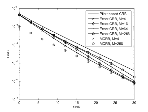
We begin by comparing the CRBs of the semi-blind approach and the pilot-based approach. In Figs. 2 and 3, we plot versus SNR the semi-blind CRB and the pilot-based CRB for parameters a𝑎a and b𝑏b, respectively. The number of pilots is L=8𝐿8L=8, and the number of transmitted data symbols is N=32𝑁32N=32. We also plot the corresponding MCRB for M=4𝑀4M=4 and M=256𝑀256M=256 in both figures. As we can see from both figures, the semi-blind CRB is substantially lower than the pilot-based bound for all 4 modulation orders. This shows that, by making use of the transmitted data symbols in addition to the pilots, the semi-blind approach can provide substantial gains in estimation accuracy over the pilot-based approach, thus providing a superior tradeoff between accuracy and spectral efficiency. We also see that the lower the modulation order the higher the achievable accuracy, with the best accuracy at M=4𝑀4M=4. In addition, Figs. 2 and 3 show that the MCRB is generally loose compared to the true CRB and is not sensitive to the modulation orders, and thus does not reflect the effect of the modulation order on the estimation accuracy. However, MCRB provides a good approximation of the true CRB at high SNR for M=4𝑀4M=4 and M=16𝑀16M=16.

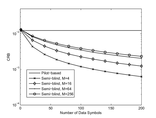
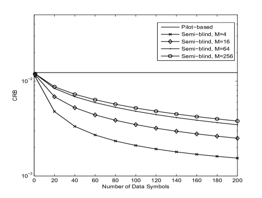
In Figs. 4 and 5, we plot the semi-blind CRBs of a𝑎a and b𝑏b versus N𝑁N, respectively. The number of pilots is L=8𝐿8L=8, and the pilot-based CRB is plotted as a reference. As we see from both plots, as N𝑁N increases, the semi-blind approach can provide increasingly better accuracy compared to the pilot-based approach. The sample size N𝑁N is constrained by the coherence time of the channel during which the channel parameters a𝑎a, b𝑏b remain fixed. Hence, the longer the channel coherence time the more attractive the semi-blind approach becomes.

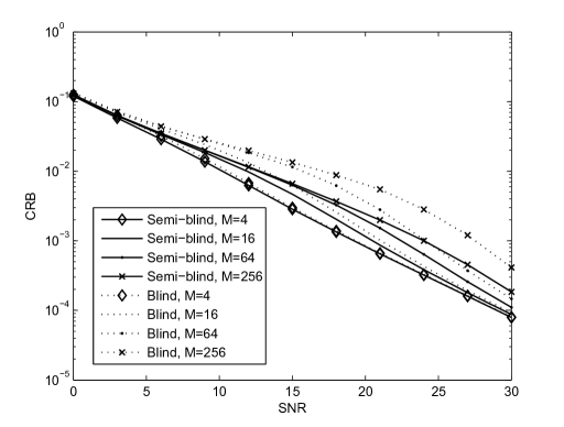
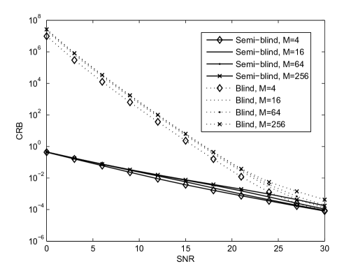
We next compare the CRBs of the semi-blind approach and the blind approach. In Figs. 6 and 7, we plot versus SNR the semi-blind and blind CRBs for parameters a𝑎a and b𝑏b, respectively. For the semi-blind case, L=8𝐿8L=8 pilots and N=32𝑁32N=32 data symbols are employed. For the blind case, N=40𝑁40N=40 data symbols are used. We see from Fig. 6 that the semi-blind approach provides better accuracy for the estimation of a𝑎a. As the modulation order increases, the gap in favor of the semi-blind approach becomes more significant. In Fig. 7, however, we see that the blind CRB for b𝑏b completely deteriorates at low SNR, reflecting the difficulty in the estimation of b𝑏b in the absence of pilots. The difference between the behaviors of the blind CRB for a𝑎a in Fig. 6 and for b𝑏b in Fig. 7 reflects the fact that in the absence of pilots the estimation of a𝑎a is an easier task than the estimation of b𝑏b due to the presence of the known self-interference symbols.

V Conclusions

In this paper, we derived the exact CRBs for semi-blind channel estimation in AF TWRNs employing square QAM modulation. As an more tractable alternative, we also derived the modified CRB. Using Monte-Carlo simulations, we showed that the semi-blind approach can provided substantial gains over the pilot-based approach. The semi-blind approach also seems to be more attractive than the blind approach, which deteriorates at low SNR. For future work, it remains to design efficient low-complexity semi-blind algorithms whose performance approaches the semi-blind CRB.

Appendix A

In this appendix, we prove (30) and (31). Recalling that uk={zkAas1k}bR+{zkAas1k}bIsubscript𝑢𝑘subscript𝑧𝑘𝐴𝑎subscript𝑠1𝑘subscript𝑏𝑅subscript𝑧𝑘𝐴𝑎subscript𝑠1𝑘subscript𝑏𝐼u_{k}=\Re\{z_{k}-Aas_{1k}\}b_{R}+\Im\{z_{k}-Aas_{1k}\}b_{I}, the second derivative of Fθ(uk)subscript𝐹𝜃subscript𝑢𝑘F_{\theta}(u_{k}) with respect to aRsubscript𝑎𝑅a_{R} is given by

2Fθ(uk)aR2=4A2{s1kb}2i=12p1βi2eγi|b|2cosh[2βiuk].\begin{split}\frac{\partial^{2}F_{\theta}(u_{k})}{\partial a_{R}^{2}}=4A^{2}\Re\{s_{1k}^{*}b\}^{2}\sum\limits_{i=1}^{2^{p-1}}\beta_{i}^{2}e^{-\gamma_{i}|b|^{2}}\cosh[2\beta_{i}u_{k}].\end{split} (64)

Thus,

𝔼{Bk(11)}=4A2{s1kb}2i=12p1βi2eγi|b|2𝔼{cosh[2βiuk]Fθ(uk)}.\begin{split}\mathbb{E}\left\{B_{k}^{(11)}\right\}=4A^{2}\Re\{s_{1k}^{*}b\}^{2}\sum\limits_{i=1}^{2^{p-1}}\beta_{i}^{2}e^{-\gamma_{i}|b|^{2}}\mathbb{E}\left\{\frac{\cosh[2\beta_{i}u_{k}]}{F_{\theta}(u_{k})}\right\}.\end{split} (65)

Using the PDF for uksubscript𝑢𝑘u_{k} in (22), we obtain:

𝔼{cosh[2βiuk]Fθ(uk)}=2πMC|b|2cosh[2βit]et2C|b|2𝑑t.𝔼2subscript𝛽𝑖subscript𝑢𝑘subscript𝐹𝜃subscript𝑢𝑘2𝜋𝑀𝐶superscript𝑏2superscriptsubscript2subscript𝛽𝑖𝑡superscript𝑒superscript𝑡2𝐶superscript𝑏2differential-d𝑡\begin{split}\mathbb{E}\left\{\frac{\cosh[2\beta_{i}u_{k}]}{F_{\theta}(u_{k})}\right\}=\frac{2}{\sqrt{\pi MC|b|^{2}}}\int\limits_{-\infty}^{\infty}\cosh[2\beta_{i}t]e^{-\frac{t^{2}}{C|b|^{2}}}dt.\end{split} (66)

Moreover, for α>0𝛼0\alpha>0, it can be verified that

eαt22δt𝑑t=παeδ2α.superscriptsubscriptsuperscript𝑒𝛼superscript𝑡22𝛿𝑡differential-d𝑡𝜋𝛼superscript𝑒superscript𝛿2𝛼\int_{-\infty}^{\infty}e^{-\alpha t^{2}-2\delta t}dt=\sqrt{\frac{\pi}{\alpha}}e^{\frac{\delta^{2}}{\alpha}}. (67)

Hence,

𝔼{cosh[2βiuk]Fθ(uk)}=2Meγi|b|2𝔼2subscript𝛽𝑖subscript𝑢𝑘subscript𝐹𝜃subscript𝑢𝑘2𝑀superscript𝑒subscript𝛾𝑖superscript𝑏2\mathbb{E}\left\{\frac{\cosh[2\beta_{i}u_{k}]}{F_{\theta}(u_{k})}\right\}=\frac{2}{\sqrt{M}}e^{\gamma_{i}|b|^{2}} (68)

and

𝔼{Bk(11)}=8A2M{s1kb}2i=12p1βi2.\mathbb{E}\left\{B_{k}^{(11)}\right\}=\frac{8A^{2}}{\sqrt{M}}\Re\{s_{1k}^{*}b\}^{2}\sum\limits_{i=1}^{2^{p-1}}\beta_{i}^{2}. (69)

Using very similar steps, we can also show that

𝔼{Hk(11)}=8A2M{s1kb}2i=12p1βi2.\mathbb{E}\left\{H_{k}^{(11)}\right\}=\frac{8A^{2}}{\sqrt{M}}\Im\{s_{1k}^{*}b\}^{2}\sum\limits_{i=1}^{2^{p-1}}\beta_{i}^{2}. (70)

Appendix B

In this appendix, we prove (39). The second derivative of Fθ(uk)subscript𝐹𝜃subscript𝑢𝑘F_{\theta}(u_{k}) with respect to bRsubscript𝑏𝑅b_{R} is given by

2Fθ(uk)bR2=i=12p1(4γi2bR22γi)eγi|b|2×cosh[2βi(bRxk+bIyk)]i=12p18βiγibRxkeγi|b|2sinh[2βi(bRxk+bIyk)]+i=12p14βi2xk2eγi|b|2cosh[2βi(bRxk+bIyk)].\begin{split}&\frac{\partial^{2}F_{\theta}(u_{k})}{\partial b_{R}^{2}}=\sum\limits_{i=1}^{2^{p-1}}(4\gamma_{i}^{2}b_{R}^{2}-2\gamma_{i})e^{-\gamma_{i}|b|^{2}}\\ &\ \ \ \ \ \ \ \ \ \ \times\cosh[2\beta_{i}(b_{R}x_{k}+b_{I}y_{k})]\\ &-\sum\limits_{i=1}^{2^{p-1}}8\beta_{i}\gamma_{i}b_{R}x_{k}e^{-\gamma_{i}|b|^{2}}\sinh[2\beta_{i}(b_{R}x_{k}+b_{I}y_{k})]\\ &+\sum\limits_{i=1}^{2^{p-1}}4\beta_{i}^{2}x_{k}^{2}e^{-\gamma_{i}|b|^{2}}\cosh[2\beta_{i}(b_{R}x_{k}+b_{I}y_{k})].\end{split} (71)

We let

T1i=12p1(4γi2bR22γi)eγi|b|2cosh[2βi(bRxk+bIyk)]T2i=12p18βiγibRxkeγi|b|2sinh[2βi(bRxk+bIyk)]T3i=12p14βi2xk2eγi|b|2cosh[2βi(bRxk+bIyk)].subscript𝑇1superscriptsubscript𝑖1superscript2𝑝14superscriptsubscript𝛾𝑖2superscriptsubscript𝑏𝑅22subscript𝛾𝑖superscript𝑒subscript𝛾𝑖superscript𝑏22subscript𝛽𝑖subscript𝑏𝑅subscript𝑥𝑘subscript𝑏𝐼subscript𝑦𝑘subscript𝑇2superscriptsubscript𝑖1superscript2𝑝18subscript𝛽𝑖subscript𝛾𝑖subscript𝑏𝑅subscript𝑥𝑘superscript𝑒subscript𝛾𝑖superscript𝑏22subscript𝛽𝑖subscript𝑏𝑅subscript𝑥𝑘subscript𝑏𝐼subscript𝑦𝑘subscript𝑇3superscriptsubscript𝑖1superscript2𝑝14superscriptsubscript𝛽𝑖2superscriptsubscript𝑥𝑘2superscript𝑒subscript𝛾𝑖superscript𝑏22subscript𝛽𝑖subscript𝑏𝑅subscript𝑥𝑘subscript𝑏𝐼subscript𝑦𝑘\begin{split}T_{1}\triangleq&\sum\limits_{i=1}^{2^{p-1}}(4\gamma_{i}^{2}b_{R}^{2}-2\gamma_{i})e^{-\gamma_{i}|b|^{2}}\cosh[2\beta_{i}(b_{R}x_{k}+b_{I}y_{k})]\\ T_{2}\triangleq&-\sum\limits_{i=1}^{2^{p-1}}8\beta_{i}\gamma_{i}b_{R}x_{k}e^{-\gamma_{i}|b|^{2}}\sinh[2\beta_{i}(b_{R}x_{k}+b_{I}y_{k})]\\ T_{3}\triangleq&\sum\limits_{i=1}^{2^{p-1}}4\beta_{i}^{2}x_{k}^{2}e^{-\gamma_{i}|b|^{2}}\cosh[2\beta_{i}(b_{R}x_{k}+b_{I}y_{k})].\end{split} (72)

We next find 𝔼{T1Fθ(uk)}𝔼subscript𝑇1subscript𝐹𝜃subscript𝑢𝑘\mathbb{E}\left\{\frac{T_{1}}{F_{\theta}(u_{k})}\right\}, 𝔼{T2Fθ(uk)}𝔼subscript𝑇2subscript𝐹𝜃subscript𝑢𝑘\mathbb{E}\left\{\frac{T_{2}}{F_{\theta}(u_{k})}\right\}, and 𝔼{T3Fθ(uk)}𝔼subscript𝑇3subscript𝐹𝜃subscript𝑢𝑘\mathbb{E}\left\{\frac{T_{3}}{F_{\theta}(u_{k})}\right\}. Using (66), we obtain

𝔼{T1Fθ(uk)}=1Mi=12p1(8γi2bR24γi).𝔼subscript𝑇1subscript𝐹𝜃subscript𝑢𝑘1𝑀superscriptsubscript𝑖1superscript2𝑝18superscriptsubscript𝛾𝑖2superscriptsubscript𝑏𝑅24subscript𝛾𝑖\begin{split}\mathbb{E}\left\{\frac{T_{1}}{F_{\theta}(u_{k})}\right\}=\frac{1}{\sqrt{M}}\sum\limits_{i=1}^{2^{p-1}}(8\gamma_{i}^{2}b_{R}^{2}-4\gamma_{i}).\end{split} (73)

We next consider 𝔼{T2Fθ(uk)}𝔼subscript𝑇2subscript𝐹𝜃subscript𝑢𝑘\mathbb{E}\left\{\frac{T_{2}}{F_{\theta}(u_{k})}\right\}. We have

𝔼{T2Fθ(uk)}=i=12p18βiγibReγi|b|2×𝔼{xksinh[2βi(bRxk+bIyk)]Fθ(bRxk+bIyk)}𝔼subscript𝑇2subscript𝐹𝜃subscript𝑢𝑘superscriptsubscript𝑖1superscript2𝑝18subscript𝛽𝑖subscript𝛾𝑖subscript𝑏𝑅superscript𝑒subscript𝛾𝑖superscript𝑏2𝔼subscript𝑥𝑘2subscript𝛽𝑖subscript𝑏𝑅subscript𝑥𝑘subscript𝑏𝐼subscript𝑦𝑘subscript𝐹𝜃subscript𝑏𝑅subscript𝑥𝑘subscript𝑏𝐼subscript𝑦𝑘\begin{split}\mathbb{E}\left\{\frac{T_{2}}{F_{\theta}(u_{k})}\right\}&=-\sum\limits_{i=1}^{2^{p-1}}8\beta_{i}\gamma_{i}b_{R}e^{-\gamma_{i}|b|^{2}}\\ &\times\mathbb{E}\left\{\frac{x_{k}\sinh[2\beta_{i}(b_{R}x_{k}+b_{I}y_{k})]}{F_{\theta}(b_{R}x_{k}+b_{I}y_{k})}\right\}\end{split} (74)

Using the PDF fX,Y(x,y)subscript𝑓𝑋𝑌𝑥𝑦f_{X,Y}(x,y) in (20), we obtain

𝔼{xksinh[2βi(bRxk+bIyk)]Fθ(bRxk+bIyk)}=4πMC×xsinh[2βi(bRx+bIy)]Fθ(bIxbRy)ex2+y2C𝑑x𝑑y=1πMC=12p1eγ|b|2x(e2βi(bRx+bIy)e2βi(bRx+bIy))×(e2β(bIxbRy)+e2β(bIxbRy))ex2+y2Cdxdy=1πMC=12p1eγ|b|2[xex2C+(2βibR+2βbI)xdx×ey2C+(2βibI2βbR)ydy+xex2C+(2βibR2βbI)x𝑑xey2C+(2βibI+2βbR)y𝑑yxex2C(2βibR2βbI)x𝑑xey2C(2βibI+2βbR)y𝑑yxex2C(2βibR+2βbI)xdxey2C(2βibI2βbR)ydy].\begin{split}&\mathbb{E}\left\{\frac{x_{k}\sinh[2\beta_{i}(b_{R}x_{k}+b_{I}y_{k})]}{F_{\theta}(b_{R}x_{k}+b_{I}y_{k})}\right\}=\frac{4}{\pi MC}\times\\ &\iint\limits_{-\infty}^{\hskip 9.04166pt\infty}x\sinh[2\beta_{i}(b_{R}x+b_{I}y)]F_{\theta}(b_{I}x-b_{R}y)e^{-\frac{x^{2}+y^{2}}{C}}dxdy\\ &=\frac{1}{\pi MC}\sum\limits_{\ell=1}^{2^{p-1}}e^{-\gamma_{\ell}|b|^{2}}\iint\limits_{-\infty}^{\hskip 9.04166pt\infty}x\left(e^{2\beta_{i}(b_{R}x+b_{I}y)}-e^{-2\beta_{i}(b_{R}x+b_{I}y)}\right)\\ &\ \ \ \ \ \ \ \ \ \ \times\left(e^{2\beta_{\ell}(b_{I}x-b_{R}y)}+e^{-2\beta_{\ell}(b_{I}x-b_{R}y)}\right)e^{-\frac{x^{2}+y^{2}}{C}}dxdy\\ &=\frac{1}{\pi MC}\sum\limits_{\ell=1}^{2^{p-1}}e^{-\gamma_{\ell}|b|^{2}}\Bigg{[}\int\limits_{-\infty}^{\infty}xe^{-\frac{x^{2}}{C}+(2\beta_{i}b_{R}+2\beta_{\ell}b_{I})x}dx\\ &\ \ \ \ \ \ \ \ \ \ \ \ \times\int\limits_{-\infty}^{\infty}e^{-\frac{y^{2}}{C}+(2\beta_{i}b_{I}-2\beta_{\ell}b_{R})y}dy\\ &+\int\limits_{-\infty}^{\infty}xe^{-\frac{x^{2}}{C}+(2\beta_{i}b_{R}-2\beta_{\ell}b_{I})x}dx\int\limits_{-\infty}^{\infty}e^{-\frac{y^{2}}{C}+(2\beta_{i}b_{I}+2\beta_{\ell}b_{R})y}dy\\ &-\int\limits_{-\infty}^{\infty}xe^{-\frac{x^{2}}{C}-(2\beta_{i}b_{R}-2\beta_{\ell}b_{I})x}dx\int\limits_{-\infty}^{\infty}e^{-\frac{y^{2}}{C}-(2\beta_{i}b_{I}+2\beta_{\ell}b_{R})y}dy\\ &-\int\limits_{-\infty}^{\infty}xe^{-\frac{x^{2}}{C}-(2\beta_{i}b_{R}+2\beta_{\ell}b_{I})x}dx\int\limits_{-\infty}^{\infty}e^{-\frac{y^{2}}{C}-(2\beta_{i}b_{I}-2\beta_{\ell}b_{R})y}dy\Bigg{]}.\end{split} (75)

In the above expression, the single integrals in x𝑥x can be evaluated using the following result which holds for α>0𝛼0\alpha>0 [14]:

teαt22δt𝑑t=πα3δeδ2α,superscriptsubscript𝑡superscript𝑒𝛼superscript𝑡22𝛿𝑡differential-d𝑡𝜋superscript𝛼3𝛿superscript𝑒superscript𝛿2𝛼\int\limits_{-\infty}^{\infty}te^{-\alpha t^{2}-2\delta t}dt=-\sqrt{\frac{\pi}{\alpha^{3}}}\delta e^{\frac{\delta^{2}}{\alpha}}, (76)

while the single integrals in y𝑦y can be evaluated using (67). After evaluating all the single integrals in (75), we finally obtain

𝔼{xsinh[2βi(bRx+bIy)]Fθ(bRx+bIy)}=4CM2p1eγi|b|2βibR.𝔼𝑥2subscript𝛽𝑖subscript𝑏𝑅𝑥subscript𝑏𝐼𝑦subscript𝐹𝜃subscript𝑏𝑅𝑥subscript𝑏𝐼𝑦4𝐶𝑀superscript2𝑝1superscript𝑒subscript𝛾𝑖superscript𝑏2subscript𝛽𝑖subscript𝑏𝑅\mathbb{E}\left\{\frac{x\sinh[2\beta_{i}(b_{R}x+b_{I}y)]}{F_{\theta}(b_{R}x+b_{I}y)}\right\}=\frac{4C}{M}2^{p-1}e^{\gamma_{i}|b|^{2}}\beta_{i}b_{R}. (77)

Therefore

𝔼{T2Fθ(uk)}=16Mi=12P1γi2bR2.𝔼subscript𝑇2subscript𝐹𝜃subscript𝑢𝑘16𝑀superscriptsubscript𝑖1superscript2𝑃1superscriptsubscript𝛾𝑖2superscriptsubscript𝑏𝑅2\mathbb{E}\left\{\frac{T_{2}}{F_{\theta}(u_{k})}\right\}=-\frac{16}{\sqrt{M}}\sum\limits_{i=1}^{2^{P-1}}\gamma_{i}^{2}b_{R}^{2}. (78)

We next consider 𝔼{T3Fθ(uk)}𝔼subscript𝑇3subscript𝐹𝜃subscript𝑢𝑘\mathbb{E}\left\{\frac{T_{3}}{F_{\theta}(u_{k})}\right\}. We have

𝔼{T3Fθ(uk)}=i=12p14βi2eγi|b|2×𝔼{xk2cosh[2βi(bRxk+bIyk)]Fθ(bRxk+bIyk)}.𝔼subscript𝑇3subscript𝐹𝜃subscript𝑢𝑘superscriptsubscript𝑖1superscript2𝑝14superscriptsubscript𝛽𝑖2superscript𝑒subscript𝛾𝑖superscript𝑏2𝔼superscriptsubscript𝑥𝑘22subscript𝛽𝑖subscript𝑏𝑅subscript𝑥𝑘subscript𝑏𝐼subscript𝑦𝑘subscript𝐹𝜃subscript𝑏𝑅subscript𝑥𝑘subscript𝑏𝐼subscript𝑦𝑘\begin{split}\mathbb{E}\left\{\frac{T_{3}}{F_{\theta}(u_{k})}\right\}&=\sum\limits_{i=1}^{2^{p-1}}4\beta_{i}^{2}e^{-\gamma_{i}|b|^{2}}\times\\ &\mathbb{E}\left\{\frac{x_{k}^{2}\cosh[2\beta_{i}(b_{R}x_{k}+b_{I}y_{k})]}{F_{\theta}(b_{R}x_{k}+b_{I}y_{k})}\right\}.\end{split} (79)

To evaluate (79), we can follow the same approach that we used in (75). However, instead of using (76), we would use the following result, which holds for α>0𝛼0\alpha>0 [14]:

t2eαt22δt𝑑t=πα5δ2eδ2α+12πα3eδ2α.superscriptsubscriptsuperscript𝑡2superscript𝑒𝛼superscript𝑡22𝛿𝑡differential-d𝑡𝜋superscript𝛼5superscript𝛿2superscript𝑒superscript𝛿2𝛼12𝜋superscript𝛼3superscript𝑒superscript𝛿2𝛼\int\limits_{-\infty}^{\infty}t^{2}e^{-\alpha t^{2}-2\delta t}dt=\sqrt{\frac{\pi}{\alpha^{5}}}\delta^{2}e^{\frac{\delta^{2}}{\alpha}}+\frac{1}{2}\sqrt{\frac{\pi}{\alpha^{3}}}e^{\frac{\delta^{2}}{\alpha}}. (80)

After some calculations (the details are skipped for brevity) we obtain

𝔼{xk2cosh[2βi(bRxk+bIyk)]Fθ(bRxk+bIyk)}=eγi|b|2(CM+2CMγibR2+4CM=12p1γbI2).𝔼superscriptsubscript𝑥𝑘22subscript𝛽𝑖subscript𝑏𝑅subscript𝑥𝑘subscript𝑏𝐼subscript𝑦𝑘subscript𝐹𝜃subscript𝑏𝑅subscript𝑥𝑘subscript𝑏𝐼subscript𝑦𝑘superscript𝑒subscript𝛾𝑖superscript𝑏2𝐶𝑀2𝐶𝑀subscript𝛾𝑖superscriptsubscript𝑏𝑅24𝐶𝑀superscriptsubscript1superscript2𝑝1subscript𝛾superscriptsubscript𝑏𝐼2\begin{split}&\mathbb{E}\left\{\frac{x_{k}^{2}\cosh[2\beta_{i}(b_{R}x_{k}+b_{I}y_{k})]}{F_{\theta}(b_{R}x_{k}+b_{I}y_{k})}\right\}=\\ &e^{\gamma_{i}|b|^{2}}\bigg{(}\frac{C}{\sqrt{M}}+\frac{2C}{\sqrt{M}}\gamma_{i}b_{R}^{2}+\frac{4C}{M}\sum\limits_{\ell=1}^{2^{p-1}}\gamma_{\ell}b_{I}^{2}\bigg{)}.\end{split} (81)

Hence,

𝔼{T3Fθ(uk)}=4Mi=12p1γi+8Mi=12p1γi2bR2+16Mi=12p1=12p1γiγ{b}2.\begin{split}\mathbb{E}\left\{\frac{T_{3}}{F_{\theta}(u_{k})}\right\}&=\frac{4}{\sqrt{M}}\sum\limits_{i=1}^{2^{p-1}}\gamma_{i}+\frac{8}{\sqrt{M}}\sum\limits_{i=1}^{2^{p-1}}\gamma_{i}^{2}b_{R}^{2}\\ &+\frac{16}{M}\sum\limits_{i=1}^{2^{p-1}}\sum\limits_{\ell=1}^{2^{p-1}}\gamma_{i}\gamma_{\ell}\Im\{b\}^{2}.\end{split} (82)

Adding (73), (78) and (82), we finally obtain

𝔼{Bk(33)}=16Mi=12p1=12p1γiγ{b}2.\mathbb{E}\left\{B_{k}^{(33)}\right\}=\frac{16}{M}\sum\limits_{i=1}^{2^{p-1}}\sum\limits_{\ell=1}^{2^{p-1}}\gamma_{i}\gamma_{\ell}\Im\{b\}^{2}. (83)

Following very similar steps, it can be shown that 𝔼{Hk(33)}=𝔼{Bk(33)}𝔼superscriptsubscript𝐻𝑘33𝔼superscriptsubscript𝐵𝑘33\mathbb{E}\left\{H_{k}^{(33)}\right\}=\mathbb{E}\left\{B_{k}^{(33)}\right\}.

Appendix C

In this appendix, we prove (47). Taking the derivative of Fθ(uk)subscript𝐹𝜃subscript𝑢𝑘F_{\theta}(u_{k}) twice with respect to τ𝜏\tau, we obtain:

2Fθ(uk)τ2=i=12p1(A4σ4βi4|b|42A4σ4Cβi2|b|2)×eγi|b|2cosh[2βiuk]+i=12p1(4A4σ4C2βi4A4σ4Cβi3|b|2)ukeγi|b|2sinh[2βiuk]+4i=12p1A4σ4C2βi2uk2eγi|b|2cosh[2βiuk].superscript2subscript𝐹𝜃subscript𝑢𝑘superscript𝜏2superscriptsubscript𝑖1superscript2𝑝1superscript𝐴4superscript𝜎4superscriptsubscript𝛽𝑖4superscript𝑏42superscript𝐴4superscript𝜎4𝐶superscriptsubscript𝛽𝑖2superscript𝑏2superscript𝑒subscript𝛾𝑖superscript𝑏22subscript𝛽𝑖subscript𝑢𝑘superscriptsubscript𝑖1superscript2𝑝14superscript𝐴4superscript𝜎4superscript𝐶2subscript𝛽𝑖4superscript𝐴4superscript𝜎4𝐶superscriptsubscript𝛽𝑖3superscript𝑏2subscript𝑢𝑘superscript𝑒subscript𝛾𝑖superscript𝑏22subscript𝛽𝑖subscript𝑢𝑘4superscriptsubscript𝑖1superscript2𝑝1superscript𝐴4superscript𝜎4superscript𝐶2superscriptsubscript𝛽𝑖2superscriptsubscript𝑢𝑘2superscript𝑒subscript𝛾𝑖superscript𝑏22subscript𝛽𝑖subscript𝑢𝑘\begin{split}&\frac{\partial^{2}F_{\theta}(u_{k})}{\partial\tau^{2}}=\sum\limits_{i=1}^{2^{p-1}}\left(A^{4}\sigma^{4}\beta_{i}^{4}|b|^{4}-2\frac{A^{4}\sigma^{4}}{C}\beta_{i}^{2}|b|^{2}\right)\\ &\hskip 64.58313pt\times e^{-\gamma_{i}|b|^{2}}\cosh[2\beta_{i}u_{k}]\\ &+\sum\limits_{i=1}^{2^{p-1}}\left(4\frac{A^{4}\sigma^{4}}{C^{2}}\beta_{i}-4\frac{A^{4}\sigma^{4}}{C}\beta_{i}^{3}|b|^{2}\right)u_{k}e^{-\gamma_{i}|b|^{2}}\sinh[2\beta_{i}u_{k}]\\ &+4\sum\limits_{i=1}^{2^{p-1}}\frac{A^{4}\sigma^{4}}{C^{2}}\beta_{i}^{2}u_{k}^{2}e^{-\gamma_{i}|b|^{2}}\cosh[2\beta_{i}u_{k}].\end{split} (84)

Since Bk(55)=2Fθ(uk)τ2Fθ(uk)superscriptsubscript𝐵𝑘55superscript2subscript𝐹𝜃subscript𝑢𝑘superscript𝜏2subscript𝐹𝜃subscript𝑢𝑘B_{k}^{(55)}=\frac{\frac{\partial^{2}F_{\theta}(u_{k})}{\partial\tau^{2}}}{F_{\theta(u_{k})}}, it is clear from (84) that we need to evaluate the terms 𝔼{cosh[2βiuk]Fθ(uk)}𝔼2subscript𝛽𝑖subscript𝑢𝑘subscript𝐹𝜃subscript𝑢𝑘\mathbb{E}\left\{\frac{\cosh[2\beta_{i}u_{k}]}{F_{\theta}(u_{k})}\right\}, 𝔼{uksinh[2βiuk]Fθ(uk)}𝔼subscript𝑢𝑘2subscript𝛽𝑖subscript𝑢𝑘subscript𝐹𝜃subscript𝑢𝑘\mathbb{E}\left\{\frac{u_{k}\sinh[2\beta_{i}u_{k}]}{F_{\theta}(u_{k})}\right\} and 𝔼{uk2cosh[2βiuk]Fθ(uk)}𝔼superscriptsubscript𝑢𝑘22subscript𝛽𝑖subscript𝑢𝑘subscript𝐹𝜃subscript𝑢𝑘\mathbb{E}\left\{\frac{u_{k}^{2}\cosh[2\beta_{i}u_{k}]}{F_{\theta}(u_{k})}\right\}. The first term is found in (68). For the second term, we have

𝔼{uksinh[2βiuk]Fθ(uk)}=2πMC|b|2tsinh[2βit]et2C|b|2𝑑t.𝔼subscript𝑢𝑘2subscript𝛽𝑖subscript𝑢𝑘subscript𝐹𝜃subscript𝑢𝑘2𝜋𝑀𝐶superscript𝑏2superscriptsubscript𝑡2subscript𝛽𝑖𝑡superscript𝑒superscript𝑡2𝐶superscript𝑏2differential-d𝑡\mathbb{E}\left\{\frac{u_{k}\sinh[2\beta_{i}u_{k}]}{F_{\theta(u_{k})}}\right\}=\frac{2}{\sqrt{\pi MC|b|^{2}}}\int\limits_{-\infty}^{\infty}t\sinh[2\beta_{i}t]e^{-\frac{t^{2}}{C|b|^{2}}}dt. (85)

The above integral can be evaluated using the result in (76), thus obtaining

𝔼{uksinh[2βiuk]Fθ(uk)}=2MC|b|2eγi|b|2βi.𝔼subscript𝑢𝑘2subscript𝛽𝑖subscript𝑢𝑘subscript𝐹𝜃subscript𝑢𝑘2𝑀𝐶superscript𝑏2superscript𝑒subscript𝛾𝑖superscript𝑏2subscript𝛽𝑖\mathbb{E}\left\{\frac{u_{k}\sinh[2\beta_{i}u_{k}]}{F_{\theta(u_{k})}}\right\}=\frac{2}{\sqrt{M}}C|b|^{2}e^{\gamma_{i}|b|^{2}}\beta_{i}. (86)

For the third term, we have

𝔼{uk2cosh[2βiuk]Fθ(uk)}=2πMC|b|2t2sinh[2βit]et2C|b|2𝑑t.𝔼superscriptsubscript𝑢𝑘22subscript𝛽𝑖subscript𝑢𝑘subscript𝐹𝜃subscript𝑢𝑘2𝜋𝑀𝐶superscript𝑏2superscriptsubscriptsuperscript𝑡22subscript𝛽𝑖𝑡superscript𝑒superscript𝑡2𝐶superscript𝑏2differential-d𝑡\mathbb{E}\left\{\frac{u_{k}^{2}\cosh[2\beta_{i}u_{k}]}{F_{\theta}(u_{k})}\right\}=\frac{2}{\sqrt{\pi MC|b|^{2}}}\int\limits_{-\infty}^{\infty}t^{2}\sinh[2\beta_{i}t]e^{-\frac{t^{2}}{C|b|^{2}}}dt. (87)

We evaluate the above integral using (80), obtaining

𝔼{uk2cosh[2βiuk]Fθ(uk)}=1Meγi|b|2(2C2|b|4βi2+C|b|2).𝔼superscriptsubscript𝑢𝑘22subscript𝛽𝑖subscript𝑢𝑘subscript𝐹𝜃subscript𝑢𝑘1𝑀superscript𝑒subscript𝛾𝑖superscript𝑏22superscript𝐶2superscript𝑏4superscriptsubscript𝛽𝑖2𝐶superscript𝑏2\mathbb{E}\left\{\frac{u_{k}^{2}\cosh[2\beta_{i}u_{k}]}{F_{\theta}(u_{k})}\right\}=\frac{1}{\sqrt{M}}e^{\gamma_{i}|b|^{2}}(2C^{2}|b|^{4}\beta_{i}^{2}+C|b|^{2}). (88)

Using (68), (86) and (88), we finally see that

𝔼{Bk(55)}=i=12p12A4σ4M(βi4|b|4+4Cβi2|b|2).𝔼superscriptsubscript𝐵𝑘55superscriptsubscript𝑖1superscript2𝑝12superscript𝐴4superscript𝜎4𝑀superscriptsubscript𝛽𝑖4superscript𝑏44𝐶superscriptsubscript𝛽𝑖2superscript𝑏2\mathbb{E}\left\{B_{k}^{(55)}\right\}=\sum\limits_{i=1}^{2^{p-1}}\frac{2A^{4}\sigma^{4}}{\sqrt{M}}\left(\beta_{i}^{4}|b|^{4}+\frac{4}{C}\beta_{i}^{2}|b|^{2}\right). (89)

The above derivation can be replicated to obtain 𝔼{Hk55}𝔼superscriptsubscript𝐻𝑘55\mathbb{E}\left\{H_{k}^{55}\right\} by replacing uksubscript𝑢𝑘u_{k} with vksubscript𝑣𝑘v_{k}, which means that 𝔼{Hk(55)}=𝔼{Bk(55)}𝔼superscriptsubscript𝐻𝑘55𝔼superscriptsubscript𝐵𝑘55\mathbb{E}\left\{H_{k}^{(55)}\right\}=\mathbb{E}\left\{B_{k}^{(55)}\right\}.

Appendix D

In this appendix, we show that 𝔼{2(𝒒;𝜽)aRaI}=0𝔼superscript2𝒒𝜽subscript𝑎𝑅subscript𝑎𝐼0\mathbb{E}\left\{\frac{\partial^{2}\mathcal{L}({\boldsymbol{q}};{\boldsymbol{\theta}})}{\partial a_{R}\partial a_{I}}\right\}=0. We have

𝔼{2(𝒒;𝜽)aRaI}=k=1N𝔼{Bk(12)Gk(12)}+k=1N𝔼{Hk12Wk(12)}.𝔼superscript2𝒒𝜽subscript𝑎𝑅subscript𝑎𝐼superscriptsubscript𝑘1𝑁𝔼superscriptsubscript𝐵𝑘12superscriptsubscript𝐺𝑘12superscriptsubscript𝑘1𝑁𝔼superscriptsubscript𝐻𝑘12superscriptsubscript𝑊𝑘12\begin{split}\mathbb{E}\left\{\frac{\partial^{2}\mathcal{L}({\boldsymbol{q}};{\boldsymbol{\theta}})}{\partial a_{R}\partial a_{I}}\right\}&=\sum\limits_{k=1}^{N}\mathbb{E}\left\{B_{k}^{(12)}-G_{k}^{(12)}\right\}\\ &+\sum\limits_{k=1}^{N}\mathbb{E}\left\{H_{k}^{12}-W_{k}^{(12)}\right\}.\end{split} (90)

To prove that 𝔼{2(𝒒;𝜽)aRaI}=0𝔼superscript2𝒒𝜽subscript𝑎𝑅subscript𝑎𝐼0\mathbb{E}\left\{\frac{\partial^{2}\mathcal{L}({\boldsymbol{q}};{\boldsymbol{\theta}})}{\partial a_{R}\partial a_{I}}\right\}=0, we will show that 𝔼{Bk(12)}=𝔼{Hk(12)}𝔼superscriptsubscript𝐵𝑘12𝔼superscriptsubscript𝐻𝑘12\mathbb{E}\left\{B_{k}^{(12)}\right\}=-\mathbb{E}\left\{H_{k}^{(12)}\right\} and 𝔼{Gk(12)}=𝔼{Wk(12)}𝔼superscriptsubscript𝐺𝑘12𝔼superscriptsubscript𝑊𝑘12\mathbb{E}\left\{G_{k}^{(12)}\right\}=-\mathbb{E}\left\{W_{k}^{(12)}\right\}. We have

2Fθ(uk)aRaI=4A2{s1kb}{s1kb}i=12p1βi2eγi|b|2×cosh[2βiuk]superscript2subscript𝐹𝜃subscript𝑢𝑘subscript𝑎𝑅subscript𝑎𝐼4superscript𝐴2superscriptsubscript𝑠1𝑘𝑏superscriptsubscript𝑠1𝑘𝑏superscriptsubscript𝑖1superscript2𝑝1superscriptsubscript𝛽𝑖2superscript𝑒subscript𝛾𝑖superscript𝑏22subscript𝛽𝑖subscript𝑢𝑘\begin{split}\frac{\partial^{2}F_{\theta}(u_{k})}{\partial a_{R}\partial a_{I}}=4A^{2}\Re\{s_{1k}^{*}b\}\Im\{s_{1k}^{*}b\}&\sum\limits_{i=1}^{2^{p-1}}\beta_{i}^{2}e^{-\gamma_{i}|b|^{2}}\\ &\times\cosh[2\beta_{i}u_{k}]\end{split} (91)

and

2Fθ(vk)aRaI=4A2{s1kb}{s1kb}i=12p1βi2eγi|b|2×cosh[2βivk].superscript2subscript𝐹𝜃subscript𝑣𝑘subscript𝑎𝑅subscript𝑎𝐼4superscript𝐴2superscriptsubscript𝑠1𝑘𝑏superscriptsubscript𝑠1𝑘𝑏superscriptsubscript𝑖1superscript2𝑝1superscriptsubscript𝛽𝑖2superscript𝑒subscript𝛾𝑖superscript𝑏22subscript𝛽𝑖subscript𝑣𝑘\begin{split}\frac{\partial^{2}F_{\theta}(v_{k})}{\partial a_{R}\partial a_{I}}=-4A^{2}\Re\{s_{1k}^{*}b\}\Im\{s_{1k}^{*}b\}&\sum\limits_{i=1}^{2^{p-1}}\beta_{i}^{2}e^{-\gamma_{i}|b|^{2}}\\ &\times\cosh[2\beta_{i}v_{k}].\end{split} (92)

Hence,

𝔼{Bk(12)}=4A2{s1kb}{s1kb}i=12p1βi2eγi|b|2×𝔼{cosh[2βiuk]Fθ(uk)},𝔼superscriptsubscript𝐵𝑘124superscript𝐴2superscriptsubscript𝑠1𝑘𝑏superscriptsubscript𝑠1𝑘𝑏superscriptsubscript𝑖1superscript2𝑝1superscriptsubscript𝛽𝑖2superscript𝑒subscript𝛾𝑖superscript𝑏2𝔼2subscript𝛽𝑖subscript𝑢𝑘subscript𝐹𝜃subscript𝑢𝑘\begin{split}\mathbb{E}\left\{B_{k}^{(12)}\right\}=&4A^{2}\Re\{s_{1k}^{*}b\}\Im\{s_{1k}^{*}b\}\sum\limits_{i=1}^{2^{p-1}}\beta_{i}^{2}e^{-\gamma_{i}|b|^{2}}\\ &\times\mathbb{E}\left\{\frac{\cosh[2\beta_{i}u_{k}]}{F_{\theta}(u_{k})}\right\},\end{split} (93)

and

𝔼{Hk(12)}=4A2{s1kb}{s1kb}i=12p1βi2eγi|b|2×𝔼{cosh[2βivk]Fθ(vk)}.𝔼superscriptsubscript𝐻𝑘124superscript𝐴2superscriptsubscript𝑠1𝑘𝑏superscriptsubscript𝑠1𝑘𝑏superscriptsubscript𝑖1superscript2𝑝1superscriptsubscript𝛽𝑖2superscript𝑒subscript𝛾𝑖superscript𝑏2𝔼2subscript𝛽𝑖subscript𝑣𝑘subscript𝐹𝜃subscript𝑣𝑘\begin{split}\mathbb{E}\left\{H_{k}^{(12)}\right\}=&-4A^{2}\Re\{s_{1k}^{*}b\}\Im\{s_{1k}^{*}b\}\sum\limits_{i=1}^{2^{p-1}}\beta_{i}^{2}e^{-\gamma_{i}|b|^{2}}\\ &\times\mathbb{E}\left\{\frac{\cosh[2\beta_{i}v_{k}]}{F_{\theta}(v_{k})}\right\}.\end{split} (94)

Since uksubscript𝑢𝑘u_{k} and vksubscript𝑣𝑘v_{k} are i.i.d., it is clear that 𝔼{Bk(12)}=𝔼{Hk(12)}𝔼superscriptsubscript𝐵𝑘12𝔼superscriptsubscript𝐻𝑘12\mathbb{E}\left\{B_{k}^{(12)}\right\}=-\mathbb{E}\left\{H_{k}^{(12)}\right\}.

We next consider 𝔼{Gk(12)}𝔼superscriptsubscript𝐺𝑘12\mathbb{E}\left\{G_{k}^{(12)}\right\} and 𝔼{Wk(12)}𝔼superscriptsubscript𝑊𝑘12\mathbb{E}\left\{W_{k}^{(12)}\right\}. To obtain 𝔼{Gk(12)}𝔼superscriptsubscript𝐺𝑘12\mathbb{E}\left\{G_{k}^{(12)}\right\} we need Fθ(uk)aRsubscript𝐹𝜃subscript𝑢𝑘subscript𝑎𝑅\frac{\partial F_{\theta}(u_{k})}{\partial a_{R}} which is given in (32) and we also need Fθ(uk)aIsubscript𝐹𝜃subscript𝑢𝑘subscript𝑎𝐼\frac{\partial F_{\theta}(u_{k})}{\partial a_{I}}, which is given by

Fθ(uk)aI=2A{s1kb}i=12p1βieγi|b|2sinh[2βiuk].subscript𝐹𝜃subscript𝑢𝑘subscript𝑎𝐼2𝐴superscriptsubscript𝑠1𝑘𝑏superscriptsubscript𝑖1superscript2𝑝1subscript𝛽𝑖superscript𝑒subscript𝛾𝑖superscript𝑏22subscript𝛽𝑖subscript𝑢𝑘\begin{split}\frac{\partial F_{\theta}(u_{k})}{\partial a_{I}}=-2A\Im\{s_{1k}^{*}b\}\sum\limits_{i=1}^{2^{p-1}}\beta_{i}e^{-\gamma_{i}|b|^{2}}\sinh[2\beta_{i}u_{k}].\end{split} (95)

Hence,

Gk(12)=Fθ(uk)aRFθ(uk)aIFθ(uk)2=4A2{s1kb}{s1kb}(i=12p1βisinh[2βiuk]Fθ(uk))2.superscriptsubscript𝐺𝑘12subscript𝐹𝜃subscript𝑢𝑘subscript𝑎𝑅subscript𝐹𝜃subscript𝑢𝑘subscript𝑎𝐼subscript𝐹𝜃superscriptsubscript𝑢𝑘24superscript𝐴2superscriptsubscript𝑠1𝑘𝑏superscriptsubscript𝑠1𝑘𝑏superscriptsuperscriptsubscript𝑖1superscript2𝑝1subscript𝛽𝑖2subscript𝛽𝑖subscript𝑢𝑘subscript𝐹𝜃subscript𝑢𝑘2\begin{split}G_{k}^{(12)}&=\frac{\frac{\partial F_{\theta}(u_{k})}{\partial a_{R}}\frac{\partial F_{\theta}(u_{k})}{\partial a_{I}}}{F_{\theta}(u_{k})^{2}}\\ &=4A^{2}\Re\{s_{1k}^{*}b\}\Im\{s_{1k}^{*}b\}\Bigg{(}\frac{\sum\limits_{i=1}^{2^{p-1}}\beta_{i}\sinh[2\beta_{i}u_{k}]}{F_{\theta}(u_{k})}\Bigg{)}^{2}.\end{split} (96)

For Wk(12)superscriptsubscript𝑊𝑘12W_{k}^{(12)}, we need Fθ(vk)aRsubscript𝐹𝜃subscript𝑣𝑘subscript𝑎𝑅\frac{\partial F_{\theta}(v_{k})}{\partial a_{R}} and Fθ(vk)aIsubscript𝐹𝜃subscript𝑣𝑘subscript𝑎𝐼\frac{\partial F_{\theta}(v_{k})}{\partial a_{I}}, which are respectively given by

Fθ(vk)aR=2A{s1kb}i=12p1βieγi|b|2sinh[2βivk],subscript𝐹𝜃subscript𝑣𝑘subscript𝑎𝑅2𝐴superscriptsubscript𝑠1𝑘𝑏superscriptsubscript𝑖1superscript2𝑝1subscript𝛽𝑖superscript𝑒subscript𝛾𝑖superscript𝑏22subscript𝛽𝑖subscript𝑣𝑘\frac{\partial F_{\theta}(v_{k})}{\partial a_{R}}=-2A\Im\{s_{1k}^{*}b\}\sum\limits_{i=1}^{2^{p-1}}\beta_{i}e^{-\gamma_{i}|b|^{2}}\sinh[2\beta_{i}v_{k}], (97)

and

Fθ(vk)aI=2A{s1kb}i=12p1βieγi|b|2sinh[2βivk].subscript𝐹𝜃subscript𝑣𝑘subscript𝑎𝐼2𝐴superscriptsubscript𝑠1𝑘𝑏superscriptsubscript𝑖1superscript2𝑝1subscript𝛽𝑖superscript𝑒subscript𝛾𝑖superscript𝑏22subscript𝛽𝑖subscript𝑣𝑘\frac{\partial F_{\theta}(v_{k})}{\partial a_{I}}=2A\Re\{s_{1k}^{*}b\}\sum\limits_{i=1}^{2^{p-1}}\beta_{i}e^{-\gamma_{i}|b|^{2}}\sinh[2\beta_{i}v_{k}]. (98)

Thus,

Wk(12)=Fθ(vk)aRFθ(vk)aIFθ(vk)2=4A2{s1kb}{s1kb}(i=12p1βisinh[2βivk]Fθ(vk))2.superscriptsubscript𝑊𝑘12subscript𝐹𝜃subscript𝑣𝑘subscript𝑎𝑅subscript𝐹𝜃subscript𝑣𝑘subscript𝑎𝐼subscript𝐹𝜃superscriptsubscript𝑣𝑘24superscript𝐴2superscriptsubscript𝑠1𝑘𝑏superscriptsubscript𝑠1𝑘𝑏superscriptsuperscriptsubscript𝑖1superscript2𝑝1subscript𝛽𝑖2subscript𝛽𝑖subscript𝑣𝑘subscript𝐹𝜃subscript𝑣𝑘2\begin{split}W_{k}^{(12)}&=\frac{\frac{\partial F_{\theta}(v_{k})}{\partial a_{R}}\frac{\partial F_{\theta}(v_{k})}{\partial a_{I}}}{F_{\theta}(v_{k})^{2}}\\ &=-4A^{2}\Re\{s_{1k}^{*}b\}\Im\{s_{1k}^{*}b\}\Bigg{(}\frac{\sum\limits_{i=1}^{2^{p-1}}\beta_{i}\sinh[2\beta_{i}v_{k}]}{F_{\theta}(v_{k})}\Bigg{)}^{2}.\end{split} (99)

Since uksubscript𝑢𝑘u_{k} and vksubscript𝑣𝑘v_{k} are i.i.d., it is clear from (96) and (99) that 𝔼{Gk(12)}=𝔼{Wk(12)}𝔼superscriptsubscript𝐺𝑘12𝔼superscriptsubscript𝑊𝑘12\mathbb{E}\left\{G_{k}^{(12)}\right\}=-\mathbb{E}\left\{W_{k}^{(12)}\right\}, which completes the proof.

References

  • [1] B. Rankov and A. Wittneben, “Spectral efficient protocols for half-duplex fading relay channels,” IEEE J. Sel. Areas Commun., vol. 25, no. 2, pp. 379–389, Feb. 2007.
  • [2] F. Gao, R. Zhang, and Y. Liang, “Optimal channel estimation and training design for two-way relay networks,” IEEE Trans. Commun., vol. 57, no. 10, pp. 3024–3033, Oct. 2009.
  • [3] B. Jiang, F. Gao, X. Gao, and A. Nallanathan, “Channel estimation and training design for two-way relay networks with power allocation,” IEEE Trans. Wireless Commun., vol. 9, no. 6, pp. 2022–2032, Jun. 2010.
  • [4] F. Roemer and M. Haardt, “Tensor-based channel estimation (TENCE) and iterative refinements for two-way relaying with multiple antennas and spatial reuse,” IEEE Trans. Signal Process., vol. 58, no. 11, pp. 5720–5735, Nov. 2010.
  • [5] F. Gao, R. Zhang, and Y. Liang, “Channel estimation for OFDM modulated two-way relay networks,” IEEE Trans. Signal Process., vol. 57, no. 11, pp. 4443–4455, Nov. 2009.
  • [6] G. Wang, F. Gao, Y.-C. Wu, and C. Tellambura, “Joint CFO and channel estimation for OFDM-based two-way relay networks,” IEEE Trans. Wireless Commun., vol. 10, no. 2, pp. 456–465, Feb. 2011.
  • [7] T.-H. Pham, Y.-C. Liang, H. Garg, and A. Nallanathan, “Joint channel estimation and data detection for MIMO-OFDM two-way relay networks,” in Proc. IEEE Global Comm. Conf. (Globecom), Miami, Florida, Dec. 2010.
  • [8] S. Abdallah and I. N. Psaromiligkos, “Blind channel estimation for amplify-and-forward two-way relay networks employing M-PSK modulation,” IEEE Trans. Signal Process., vol. 60, no. 7, pp. 3604–3615, Jul. 2012.
  • [9] S. Abdallah and I. Psaromiligkos, “Partially-blind estimation of reciprocal channels for af two-way relay networks employing M-PSK modulation,” IEEE Trans. Wireless Commun., vol. 11, no. 5, pp. 1649 –1654, May 2012.
  • [10] F. Bellili, A. Stephenne, and S. Affes, “Cramer-Rao lower bounds for NDA SNR estimates of square QAM modulated transmissions,” IEEE Trans. Commun., vol. 58, no. 11, pp. 3211–3218, Nov. 2010.
  • [11] F. Gini and R. Reggiannini, “On the use of Cramer-Rao-like bounds in the presence of random nuisance parameters,” IEEE Trans. Commun., vol. 48, no. 12, pp. 2120–2126, Dec. 2000.
  • [12] J. Gorman and A. Hero, “Lower bounds for parametric estimation with constraints,” IEEE Trans. Inf. Theory, vol. 36, no. 6, pp. 1285–1301, Nov. 1990.
  • [13] Y. Chen and C. Tellambura, “Performance analysis of l-branch equal gain combiners in equally correlated rayleigh fading channels,” IEEE Comm. Lett., vol. 8, no. 3, pp. 150–152, 2004.
  • [14] M. Abramowitz and E. Irene A. Stegun, Handbook of Mathematical Functions, 9th ed.   New York: Dover Publications, 1970.
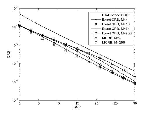
Refer to caption
Figure 2: Semi-blind and pilot-based CRBs for the estimation of a𝑎a plotted versus SNR for N=32𝑁32N=32 and L=8𝐿8L=8, and for M=4, 16, 64, 256𝑀41664256M=4,\ 16,\ 64,\ 256. We also plot MCRBa𝑀𝐶𝑅subscript𝐵𝑎MCRB_{a} for M=4𝑀4M=4 and M=256𝑀256M=256.
Refer to caption
Figure 3: Semi-blind and pilot-based CRBs for the estimation of b𝑏b plotted versus SNR for N=32𝑁32N=32 and L=8𝐿8L=8, and for M=4, 16, 64, 256𝑀41664256M=4,\ 16,\ 64,\ 256. We also plot MCRBb𝑀𝐶𝑅subscript𝐵𝑏MCRB_{b} for M=4𝑀4M=4 and M=256𝑀256M=256.
Refer to caption
Figure 4: Semi-blind CRB for the estimation of a𝑎a plotted versus N𝑁N for L=8𝐿8L=8, and for M=4, 16, 64, 256𝑀41664256M=4,\ 16,\ 64,\ 256. The pilot-based CRB is shown as a reference.
Refer to caption
Figure 5: Semi-blind CRB for the estimation of b𝑏b plotted versus N𝑁N for L=8𝐿8L=8, and for M=4, 16, 64, 256𝑀41664256M=4,\ 16,\ 64,\ 256. The pilot-based CRB is shown as a reference.
Refer to caption
Figure 6: Semi-blind and blind CRBs for the estimation of a𝑎a plotted versus SNR for M=4, 16, 64, 256𝑀41664256M=4,\ 16,\ 64,\ 256. We use N=32𝑁32N=32 data symbols and L=8𝐿8L=8 pilots for the semi-blind case, and we use N=40𝑁40N=40 data symbols for the blind case.
Refer to caption
Figure 7: Semi-blind and blind CRBs for the estimation of b𝑏b plotted versus SNR for M=4, 16, 64, 256𝑀41664256M=4,\ 16,\ 64,\ 256. We use N=32𝑁32N=32 data symbols and L=8𝐿8L=8 pilots for the semi-blind case, and we use N=40𝑁40N=40 data symbols for the blind case.