Potential of a Neutrino Detector in the ANDES Underground Laboratory for Geophysics and Astrophysics of Neutrinos

Abstract

The construction of the Agua Negra tunnels that will link Argentina and Chile under the Andes, the world longest mountain range, opens the possibility to build the first deep underground laboratory in the Southern Hemisphere. This laboratory has the acronym ANDES (Agua Negra Deep Experiment Site) and its overburden could be as large as $\sim 1.7$ km of rock, or 4500 mwe, providing an excellent low background environment to study physics of rare events like the ones induced by neutrinos and/or dark matter. In this paper we investigate the physics potential of a few kiloton size liquid scintillator detector, which could be constructed in the ANDES laboratory as one of its possible scientific programs. In particular, we evaluate the impact of such a detector for the studies of geoneutrinos and galactic supernova neutrinos assuming a fiducial volume of 3 kilotons as a reference size. We emphasize the complementary roles of such a detector to the ones in the Northern Hemisphere neutrino facilities through some advantages due to its geographical location.

I Introduction

After the pioneering neutrino experiments performed at Homestake (South Dakota, USA) Cleveland:1998nv and Kamioka (Gifu, Japan) Hirata:1987hu , and the great achievements by Super-Kamiokande sk-atm , KamLAND KamLAND , both in Kamioka, and SNO Ahmad:2002jz (Sudbury, Canada) experiments which provided strong evidence of neutrino oscillation, it has been well recognized that deep underground laboratories can offer an excellent environment for neutrino experiments as well as for a variety of interesting scientific programs which include several different fields, from particle physics, astrophysics, nuclear physics, to biology, geology and geophysics. See Smith-review-taup11 for a review of the world’s underground laboratories.

Experiments searching for very rare events, such as the ones induced by neutrinos or dark matter interactions, proton decay or performing low energy nuclear cross section measurements, cannot be carried out at the Earth’s surface mainly due to the backgrounds induced by cosmic rays. For these experiments a reduction of the cosmogenic backgrounds is crucial. This can be accomplished by having enough rock overburden, making clear the reason for going deep underground.

Recently it was proposed Andes-Website to build the first underground laboratory in the Southern Hemisphere by digging a cave off one of the two 14 km long Agua Negra tunnels. These tunnels will be constructed under the Andes, the longest continental mountain range in the world, to connect Chile’s region IV and Argentina’s San Juan province. They will provide a link between the port of Coquimbo, Chile (on the Pacific Ocean), and the port of Porto Alegre, Brazil (on the Atlantic Ocean), and several nearby cities, in order to facilitate trade between Asia and MERCOSUR (Mercado Común del Sur or Common Southern Market in English) which is an economic and political agreement among Argentina, Brazil, Paraguay and Uruguay. While the exact location of the laboratory inside the tunnel is still under study, the rock overburden could be as large as $\sim$ 1.7 km, allowing to significantly reduce backgrounds from cosmic ray origin. The name given to the proposed laboratory is ANDES (Agua Negra Deep Experiment Site).

If such an underground laboratory is constructed, it could provide a variety of interesting scientific opportunities for dedicated studies of neutrinos, dark matter searches and nuclear astrophysics Andes-Website , among other things. The current preliminary design of the ANDES laboratory is as follows Bertou-workshop3 . There will be two large experimental halls with dimensions of $21\times 23\times 50$ m³ and $16\times 14\times 40$ m³, and one smaller hall for offices and multidisciplinary experiments with size of $17\times 15\times 25$ m³. In addition, there will be two experimental pits, one is a smaller ultra-low radiation pit with 8 m of diameter and 9 m of height, the other is a large single experiment pit with 30 m of diameter and 30 m of height. We are particularly interested in this large pit where a liquid scintillator detector could be installed and used in a possible neutrino program for the ANDES.

As demonstrated by KamLAND KamLAND , Borexino Borexino-solar ; Borexino-geo , as well as the recent $\theta_{13}$ reactor experiments, Double Chooz Abe:2011fz , Daya Bay An:2012eh and RENO collaboration:2012nd , liquid scintillator detectors have a very good capability to observe $\bar{\nu}_{e}$ through the inverse beta decay reaction, $\bar{\nu}_{e}+p\to n+e^{+}$. They also can work with a low energy threshold and provide good energy resolution. As a possible candidate for the ANDES neutrino detector one could consider a KamLAND KamLAND , Borexino Alimonti:2000xc or SNO+ Kraus:2010zzb like liquid scintillator detector with a fiducial mass of a few kt. In this paper, we assume a liquid scintillator detector based on alkyl benzene (C₆H₅C₁₂H₂₅), which will be used for the SNO+ detector, with a fiducial mass of 3 kt, containing $\sim 2.2\times 10^{32}$ free protons as targets, as our reference neutrino detector at the ANDES, unless otherwise stated.

We focus on the detection of neutrinos originating from some radioactive elements inside the Earth, the so called geoneutrinos, and neutrinos coming from a core collapse supernova (SN) in our galaxy (hereafter SN implies core collapse supernova). For reviews on these subjects, see, for example, Refs. Fiorentini:2007te ; Enomoto-thesis-2005 for geoneutrinos and Ref. Raffelt:2010zza for SN neutrinos. Some preliminary results of this work can be found in Refs. Andes-talk1 ; Andes-talk2 ; Andes-talk3 .

The first successful observations of geoneutrinos by KamLAND Araki:2005qa and Borexino Bellini:2010hy open a new window to study the chemical composition of the Earth. It is believed that the geoneutrino flux has a local dependency Fiorentini:2007te , hence having more detectors in different parts of the Earth capable of measuring such neutrinos is highly welcome. Since the ANDES laboratory is surrounded by a thick continental crust, we expect a geoneutrino flux larger than at Kamioka or Gran Sasso, which is interesting to confirm experimentally. Moreover, compared to other existing underground laboratories, there are very few nuclear reactors around the ANDES location - a valuable advantage as reactor neutrinos are one of the main backgrounds for the measurement of geoneutrinos.

After the historical observations of SN neutrinos from SN1987A occurred in the Large Magellanic Cloud by Kamiokande Hirata:1987hu , IMB Bionta:1987qt , and Baksan Alekseev:1988gp detectors, it is well understood that such SN neutrinos can play a very important role in uncovering the physics of supernovae as well as some properties of the neutrinos themselves, such as mass, lifetime, magnetic moment, etc Raffelt:1996wa . The low rate of nearby SN, which occurs close enough to the Earth so that it can be observed also by neutrinos, is another strong reason for having as many simultaneously operating neutrino detectors as possible, in order to take advantage of such a rare opportunity. The additional new neutrino detector would also help in making a quick alert to astronomers about the occurrence of a nearby SN event through the SuperNova Early Warning System (SNEWS) network Antonioli:2004zb .

The ANDES neutrino detector, if constructed, can certainly make some relevant contribution to SN neutrino observations. Furthermore, the location of the ANDES laboratory in the Southern Hemisphere can provide a better chance to observe the Earth matter effect for SN neutrinos by combining with other detectors in the Northern Hemisphere. If Earth matter effect is observed, the neutrino mass hierarchy may be determined and, at the same time, evidence that different SN neutrino flavors manifest significantly different energy spectra can be provided.

The organization of this paper is as follows. In Sec. II we discuss in detail the potential of the ANDES neutrino detector for geoneutrino observations. In Sec. III we discuss SN neutrino observation at the ANDES neutrino detector. Sec. IV is devoted to discussions and conclusions of our results. While we follow previous works for most of the calculations done in this work, for the sake of completeness and to be self-contained, we describe some details of our numerical calculations in the Appendices.

II Geoneutrinos

II.1 Introduction

The deep interior of the Earth, governed by high pressure and temperature, is the last frontier on our planet, which has not yet been explored by a human being. The deepest hole ever made so far is 12.3 km down from the Earth’s surface Fiorentini:2007te , only about 0.1% of the Earth’s diameter, and so even the top of the mantle has not yet been reached. In the near future, a direct access to the upper mantle will be possible as part of the missions of the international scientific research program named IODP (Integrated Ocean Drilling Program)IODP . However, to reach the lower part of the Earth’s mantle, located at a depth of about 660 km from the surface, seems to be an impossible task.

So far, there are basically two different approaches to overcome the direct inaccessibility of the Earth’s underground below 10 km: seismology and geochemistry. Seismological data permit us to indirectly reconstruct the matter density profile of the whole Earth. Geochemistry, however, can only access the composition of the Earth close to the surface. For that one uses various rock samples coming from the Earth’s crust as well as very limited samples from the top of the mantle, thanks to volcanic activity and orogeny.

In 2005 the KamLAND experiment Araki:2005qa reported for the first time the detection of $\bar{\nu}_{e}$ coming from the decay chains of the radioactive isotopes ²³⁸U and ²³²Th in the Earth, by using the inverse beta decay reaction $\bar{\nu}_{e}+p\to n+e^{+}$. These geoneutrinos can provide useful information not only relevant to the Earth’s interior chemical composition but also shed light on the source of the terrestrial heat production, opening a window to a new scientific field, neutrino geophysics or neutrino geoscience. In 2010, another experiment, Borexino, located in the Gran Sasso Laboratory in Italy also reported the measurement of geoneutrinos Bellini:2010hy , further contributing to the start of neutrino geoscience. A partial list of previous works on geoneutrinos can be found in Refs. Krauss:1983zn ; Raghavan:1997gw ; geo-nu-fiorentini ; geo-nu-bari ; Nunokawa:2003dd ; Fiorentini:2007te .

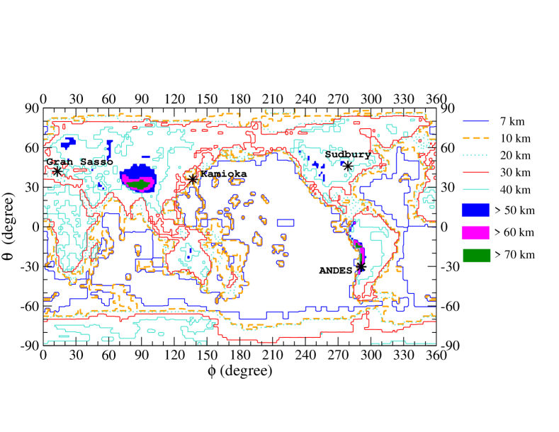
Figure 1: Isocontour map of the Earth’s crust thickness (in km) in the plane of $\theta$ (latitude)-$\phi$ (longitude) based on the model found in Ref. geoneutrinos-gabi-etal . The positions of the Gran Sasso, Kamioka, Sudbury and ANDES underground laboratories are also indicated by asterisks.

It is estimated that the entire Earth generates about 40 TW, corresponding to $\sim$ 10,000 reactors. It has been considered that most (or all) of the heat is generated by the energy deposited by the decay of radioactive elements like U, Th and K in the Earth’s interior. By measuring geoneutrinos, which are the direct product of such decays, one can infer the total amount of U and Th inside the Earth. We note that the amount of K can not be inferred directly by the current detection method since the energy of geoneutrinos coming from K is below the threshold of the inverse beta decay reaction.

The measured geoneutrino flux, reported recently by the KamLAND experiment KamLAND-nature-geo2011 , is $4.3^{+1.2}_{-1.1}\times 10^{6}$ cm^-2s^-1. By taking into account neutrino oscillations, this corresponds to a total emitted flux of $7.4^{+2.1}_{-1.9}\times 10^{6}$ cm^-2s^-1. On the other hand, Borexino experiment Borexino-geo reported in terms of the observed number of events, $3.9^{+1.6}_{-1.3}(^{+5.8}_{-3.2})$ events/(100 ton yr) at 68% (99.73 %) CL. This result is about 70 % higher than that obtained by KamLAND KamLAND-nature-geo2011 , though both results are consistent with each other within the experimental and theoretical uncertainties.

By combining the results from KamLAND and Borexino, the observed geoneutrino flux corresponds to a heat production of $20^{+8.8}_{-8.6}$ TW KamLAND-nature-geo2011 . While Borexino seems to favor, KamLAND results disfavor the so called fully radiogenic model, the model where all the terrestrial heat comes from the decay of the radioactive elements in the Earth crust and mantle. KamLAND alone disfavors this model at 98.1% CL while the combined data of these two experiments slightly reduces the significance of this rejection to 97.2% CL KamLAND-nature-geo2011 .

II.2 Why measure geoneutrinos in the ANDES?

For various reasons it would be very interesting if the measurement of geoneutrinos can also be done at the ANDES Laboratory. First we note that the location of the ANDES laboratory, 30^∘15’ S and 69^∘53’ W, is surrounded by the Andes mountain range which means that the thickness of the crust around the laboratory is significantly larger than the average Earth crustal thickness, leading to an expected larger geoneutrino flux. This is because in the Earth’s crust the concentration of U and Th is expected to be significantly larger than in the deeper mantle.

In Fig. 1 we present the isocontour map of the Earth crust thickness based on the model found in Ref. geoneutrinos-gabi-etal . In Fig. 2 we present the magnified version of Fig. 1 around the ANDES laboratory. From these figures, we can appreciate the difference of the local crust thickness around the ANDES laboratory in comparison with other locations on our planet. Indeed, roughly speaking, the expected geoneutrino flux at the ANDES laboratory site is larger than that for KamLAND and Borexino by about 30 % and 20 %, respectively, as we will see below. It is important to confirm such local dependence of the geoneutrino fluxes. Because of such a local (site) dependence, it would be also very interesting to measure the geoneutrino flux at a location surrounded by oceanic crust, such as in Hawaii Hanohano , where the main contribution to the geoneutrino flux is expected to come from the decay of radioactive elements in the mantle.

Figure 2: Same as in Fig. 1 but around the ANDES laboratory.

Second, there are very few nuclear reactors near the ANDES laboratory which is a great advantage for measuring geoneutrinos. As it is well know from the results of the KamLAND experiment, low energy $\bar{\nu}_{e}$ produced by nuclear reactors is one of the most important backgrounds for geoneutrino observation. Indeed, the Borexino detector, despite being smaller than KamLAND, demonstrated so far a better performance than KamLAND as far as geoneutrino measurements are concerned. This seems to be due to the fact that Borexino, located in the middle of Italy where there are no nearby reactors, is exposed to a much lower $\bar{\nu}_{e}$ background from reactor origin.

Taking into account the nearest Argentinian nuclear reactors, the Embase 2.1 GW (thermal power) as well as the Atucha I 1.2 GW and Atucha II 2.1 GW reactors, which are located, respectively, 560 km and 1080 km away from the ANDES Laboratory, we have estimated a total reactor background of 8.8 events/yr/3 kt and 2.2 events/yr/3 kt in the geoneutrino energy range. These numbers are given in the absence of neutrino oscillations, which will further reduce them if taken into account. Though we have considered only the contribution from these nearby reactors, our estimation is similar to the one which can be inferred from Fig. 2 of Ref. Lasserre:2010my which shows the world map of the isocontours of the expected number of events induced by neutrinos coming from 201 nuclear reactor power stations all over the world. The reactor neutrino background we found for ANDES is more than 10 times smaller than the one expected for Borexino, 5.7 events/yr/100 tons (total number of reactor $\bar{\nu}_{e}$ induced events in the presence of oscillation) Borexino-geo .

II.3 Calculating the geoneutrino flux

We follow our (two of the authors of this paper) previous work Nunokawa:2003dd with some update and improvements, in order to compute the differential flux of $\bar{\nu}_{e}$ produced in the decay chain of radioactive isotopes ²³⁸U and ²³²Th that will be measured at a detector position $\mathbf{r}$ on the Earth, which can be expressed by the following integral performed over the Earth’s volume $V_{\oplus}$,

$$\frac{d\Phi_{\bar{\nu}_{e}}(\mathbf{r})}{dE_{\bar{\nu}_{e}}}=\sum_{k=\text{U,Th}}\int_{V_{\oplus}}d^{3}\mathbf{r}^{\prime}\frac{\rho(\mathbf{r}^{\prime})}{4\pi|\mathbf{r}-\mathbf{r}^{\prime}|^{2}}\,\frac{c_{k}(\mathbf{r}^{\prime})n_{k}}{\tau_{k}m_{k}}\,\times P_{\bar{\nu}_{e}}(E_{\bar{\nu}_{e}},|\mathbf{r}-\mathbf{r}^{\prime}|)\times f_{k}(E_{\bar{\nu}_{e}}),$$ (1)

where $\rho(\mathbf{r})$ is the matter density, $c_{k}(\mathbf{r})$, $\tau_{k}$, $m_{k}$ and $n_{k}$ are, respectively, the mass abundance, half-life, atomic mass and the number of $\bar{\nu}_{e}$ emitted per decay chain corresponding to element $k=^{238}$U, ²³²Th, $f_{k}(E_{\bar{\nu}_{e}})$ is the normalized spectral function for element $k$ spectrum .

We will assume the concentrations of U and Th, $c_{k}(\mathbf{r})$, take different values in the Earth’s crust and mantle layers as given in Table 1. These are our reference values which are based on Ref. Enomoto-thesis-2005 . Oceanic and continental Earth’s crust are divided, respectively, into two and four layers whereas the Earth’s mantle is divided into two layers (see Table 1). We assume no U and Th in the Earth’s core. The so called fully radiogenic model assumes higher U, Th and K abundances in the mantle in order that the total observed Earth’s heat can be fully explained by the decay of these radio active elements. We have used the Earth crust model taken from Ref. geoneutrinos-gabi-etal (shown in Figs. 1 and 2).

$P_{\bar{\nu}_{e}}(E_{\bar{\nu}_{e}},|\mathbf{r}-\mathbf{r}^{\prime}|)$ describes the survival probability of $\bar{\nu}_{e}$ produced at $\mathbf{r}^{\prime}$ but measured at $\mathbf{r}$, which can be averaged out, as a good approximation, and bring out from the integral the term:

$$\langle P_{\bar{\nu}_{e}}\rangle\simeq\left\langle\sin^{4}\theta_{13}\right.\left.+\cos^{4}\theta_{13}\left(1-\sin^{2}2\theta_{12}\sin^{2}\left[\frac{\Delta m^{2}_{21}}{4E_{\bar{\nu}_{e}}}|\mathbf{r}-\mathbf{r}^{\prime}|\right]\right)\right\rangle\simeq\sin^{4}\theta_{13}+\cos^{4}\theta_{13}\left(1-\frac{1}{2}\sin^{2}2\theta_{12}\right)\simeq 0.55,$$ (2)

where $\Delta m^{2}_{21}\equiv m_{2}^{2}-m_{1}^{2}\simeq 7.5\times 10^{-5}$ eV², $m_{1}$, $m_{2}$ being the neutrino masses, $\sin^{2}\theta_{12}=0.31$ and $\sin^{2}\theta_{13}=0.025$ global-analysis . In this work we use the standard neutrino mixing parameterization found in Ref. Nakamura:2010zzi .

Layer	$c_{\rm U}$ ($\mu$ g/g)	$c_{\rm Th}$ ($\mu$ g/g)
Oceanic Sediment	1.68	6.91
Oceanic Crust	0.1	0.22
Continental Sediment	2.8	10.7
Upper Continental Crust	2.8	10.7
Middle Continental Crust	1.6	6.1
Lower Continental Crust	0.2	1.2
Upper Mantle	0.012	0.048
Lower Mantle	0.012	0.048

Table 1: U and Th mass abundances in different layers of the Earth’s crust and mantle used in this work Enomoto-thesis-2005 . In the Earth’s core these mass abundances are assumed to be zero.

Figure 3: Cumulative flux of geoneutrinos coming from the decay of ²³⁸U as a function of the distance from the ANDES neutrino detector.

We have computed the expected total fluxes of $\bar{\nu}_{e}$ at ANDES coming, respectively, from U and Th to be, $\Phi_{\rm U}=5.58\times 10^{6}$ cm^-2 s^-1 ($3.04\times 10^{6}$ cm^-2 s^-1) and $\Phi_{\rm Th}=4.78\times 10^{6}$ cm^-2 s^-1 ($2.60\times 10^{6}$ cm^-2 s^-1) without neutrino oscillation (with oscillation). In Fig. 3 we present the geoneutrino cumulative flux for the U chain as a function of the distance from the ANDES laboratory. We observe that 50% of the flux comes from $\simeq$ 200 km from the detector and about 20% of the flux comes from the mantle.

In Fig. 4 we show our expectations for the total oscillated geoneutrino flux at Kamioka, Gran Sasso, SNO, Hawaii, Pyhäsalmi and ANDES, discriminating the crust and mantle contributions in each case. Pyhäsalmi in Finland is a possible site for the proposed 50 kt LENA neutrino detector Wurm:2011zn . We also show KamLAND KamLAND-nature-geo2011 and Borexino data Bellini:2010hy points to compare with the precision of the expected measurement by ANDES after 5 years of data taking. According to Ref. Fiorentini:2012yk the current KamLAND and Borexino results combined imply the geoneutrinos from the mantle have been observed at 2.4 $\sigma$ CL. Clearly ANDES by itself, after 5 years, is able to establish the mantle geoneutrino component at a level of about 3 $\sigma$ or better.

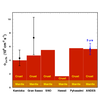
Figure 4: Total geoneutrino flux (oscillated) expected at Kamioka, Gran Sasso, SNO, Hawaii, Pyhäsalmi and ANDES. We show the expected contribution from crust and mantle, in each case, as well as KamLAND KamLAND-nature-geo2011 and Borexino data Bellini:2010hy points. We also show (in blue) the precision of the expected measurement by ANDES after 5 years at 1 and 3 $\sigma$ CL.

Let us now discuss the expected number of geoneutrino induced events at the ANDES neutrino detector. For one year of operation ($3\times 10^{7}$ s) and 80% detector efficiency, we have calculated the total number of geonetrinos expected at the ANDES reference detector to be 82.4 (64.8 from U, 17.6 from Th). About 16 of these events would be from the mantle and 35 events would have $E_{\nu}>$ 2.3 MeV, coming exclusively from the U chain. To illustrate the site dependence we show in Table 2 our estimation for the corresponding number of geoneutrino events in different locations assuming the same reference detector (the same number of free protons, efficiency and exposure). From this table we see that the expected number of geoneutrino events at the ANDES location is comparable to SNO and to Pyhäsalmi.

Location	Number from U	Number from Th	Total
Gran Sasso	53.8	14.7	68.5
Kamioka	45.7	12.4	58.1
Hawaii	18.5	5.0	23.5
Sudbury	63.2	17.2	80.4
Pyhäsalmi	66.1	18.0	84.1
ANDES	64.8	17.6	82.4

Table 2: Expected number of geoneutrino events for our reference 3 kt liquid scintillator detector operating during a year with 80% efficiency at different locations.

Such a detector operating during 10 years could accumulate more than 800 geonetrino events (160 from the mantle alone), allowing not only for a better determination of U and Th mass abundances in the crust and mantle but also for the investigation of their presence in the Earth’s core. Clearly if an even larger detector, say 10 kt, could be envisaged the scientific reach could be even more significant.

III Supernova Neutrinos

III.1 Preliminaries

If we consider the entire universe, the SN event rate is not so low, several SN explosions per second. However, if we restrict to our galaxy, more interesting in terms of SN neutrino observations, the estimated event rate of such nearby SN drops down to about $\raise 1.29167pt\hbox{$\;<$\kern-7.5pt\raise-4.73611pt\hbox{$\sim\;$}}3$ per century Bergh:1991ek ; Tammann:1994ev ; Diehl:2006cf . In fact, in last $\sim$ 30 years, since when the Baksan neutrino detector started to operate in 1980, only neutrinos from the explosion of SN1987A in the Large Magellanic Cloud, one of the satellite galaxies of the Milky Way, were observed by the Kamiokande Hirata:1987hu , IMB Bionta:1987qt , and Baksan Alekseev:1988gp neutrino detectors.

Fortunately today, compared to that epoch, we are better prepared for SN neutrino observations as there are much larger neutrino detectors, such as Super-Kamiokande Ikeda:2007sa and IceCube Abbasi:2011ss , which are currently in operation. However, since the nearby SN rate is quite low, it is better to have as many neutrino detectors as possible, to be ready for the next SN event. This will maximize the chance to obtain as much information as possible on SN neutrinos, leading to a better understanding of the SN explosion dynamics.

Since the last galactic SN, SN1604, was observed more than 400 years ago and we do not know when exactly the next one will occur, it is important to have neutrino detectors with larger running time. Having many neutrino detectors is also helpful in forming a network like SNEWS Antonioli:2004zb that will readily alert the astronomers about the occurrence of a nearby SN event enabling them not to miss the initial phase of the time evolution of the SN light curve.

It is theoretically expected Bethe:1990mw that almost all ($\sim 99$ %) the energy released by gravitational collapse is carried away in the form of neutrinos, which was consistent with the observed data of SN1987A neutrinos. Roughly speaking, the neutrino emission from a SN explosion can be divided into four periods: (i) the infall phase, which starts several tens of ms before the bounce; (ii) the shock breakout neutronization burst, which lasts up to a few tens of ms after the bounce; (iii) the accretion phase, during from a few tens of ms up to several hundreds of ms after the bounce and (iv) the Kelving-Helmholtz cooling phase, during up to $\sim$ 10-20 s after the bounce.

Emission of $\nu_{e}$ starts during the infall phase, though the luminosity is not yet so large. In the neutronization burst phase, there is a strong $\nu_{e}$ burst in a very short period of time, $\sim 10$ ms, and the emission of the other flavors, as well as of $\bar{\nu}_{e}$, is suppressed. During the accretion phase, the fluxes of $\nu_{e}$ and $\bar{\nu}_{e}$ are expected to be significantly larger than that of the other flavors and the energy hierarchy $\langle E_{\nu_{e}}\rangle<\langle E_{\bar{\nu}_{e}}\rangle<\langle E_{\nu_{x}}\rangle$ is expected. Here we use the notation $\nu_{x}$ to refer to any non-electron neutrino since for our purpose they can be treated, in good approximation, as a single species. During the cooling phase the emission of all flavors of neutrinos and antineutrinos, with similar luminosities, is predicted.

It is considered that the energy spectra of SN neutrinos can be approximately described by Fermi-Dirac distributions with some non-zero chemical potential, which is in general necessary to account for the non-thermal feature of the SN neutrino spectra. In this work, for any flavor, $\nu_{\alpha}$, we will use the following parameterization, which is based on the numerical simulations by the Garching group Keil:2002in ; Keil:2003sw ; Buras:2002wt , for the SN neutrino spectra at the Earth in the absence of neutrino oscillation,

$$F^{0}_{\nu_{\alpha}}(E)=\frac{1}{4\pi D^{2}}\ \frac{\Phi_{\nu_{\alpha}}}{\left\langle E_{\nu_{\alpha}}\right\rangle}\,\frac{\beta_{\alpha}^{\beta_{\alpha}}}{\Gamma(\beta_{\alpha})}\left[\frac{E}{\left\langle E_{\nu_{\alpha}}\right\rangle}\right]^{\beta_{\alpha}-1}\exp\left[-\beta_{\alpha}\frac{E}{\left\langle E_{\nu_{\alpha}}\right\rangle}\right],\,$$ (3)

where $D$ is the distance to the SN, $\Phi_{\nu_{\alpha}}$ is the total number of $\nu_{\alpha}$ emitted, $\left\langle E_{\nu_{\alpha}}\right\rangle$ is the average energy of $\nu_{\alpha}$ and $\beta_{\alpha}$ is a parameter which describes the deviation from a thermal spectrum (pinching effect) that can be taken to be $\sim 2-4$, $\Gamma(\beta_{\alpha})$ is the gamma function.

This parameterization seems to describe better the SN neutrino spectra obtained by numerical simulations. We note, however, that our results would not change much even if we had used instead Fermi-Dirac distributions with a non-zero chemical potential. During the neutrino emission, as many SN simulations indicate, the shape of $F^{0}_{\nu_{\alpha}}(E)$ is expected to change in time, which means that the average neutrino energies as well as their luminosities are, in general, functions of time. We do not explore this feature in this work .

For the sake of discussion, unless otherwise explicitly stated, we use the SN parameters summarized in Table 3 as our reference values. We assume that the total energy released by SN neutrinos is 3$\times 10^{53}$ erg, which is equally divided by 6 species of active neutrinos, and consider 10 kpc as a typical distance to the SN. The chance that the actual distance could be even smaller, say 5 kpc, seems, however, to be not so small. This can be seen in Fig. 16 in the Appendix C, where the expected SN distributions as a function of the distance from the Earth, based on the distribution models considered in Mirizzi:2006xx , are shown.

Reference SN parameters

Distance to the SN : D = 10 kpc

Spectra parmetrization in Eq.(3) with $\beta_{\alpha}$ = 4 for all flavors

$\langle E_{\nu_{e}}\rangle$ = 12 MeV    $\langle E_{\bar{\nu}_{e}}\rangle$ = 15 MeV    $\langle E_{\nu_{x}}\rangle$ = 18 MeV

$E^{\text{tot}}_{\nu_{\alpha}}=\langle E_{\nu_{\alpha}}\rangle\Phi_{\nu_{\alpha}}=5\times 10^{52}$ erg   for all flavor

Table 3: Reference SN parameters to be used throughout this paper, unless otherwise explicitly stated.

Due to neutrino oscillations in the SN envelope, the SN neutrino flux spectra at Earth are in general expected not to be given by Eq. (3) but by flavor mixtures (superpositions) of them. Without loss of generality, the flux spectrum of observable $\bar{\nu}_{e}$ at the Earth can be expressed as

$$F_{\bar{\nu}_{e}}(E)=\bar{p}(E)\,F_{\bar{\nu}_{e}}^{0}(E)+[1-\bar{p}(E)]F_{\bar{\nu}_{x}}^{0}(E)\,,$$ (4)

where $F_{\bar{\nu}_{e}}^{0}(E)$ and $F_{\bar{\nu}_{x}}^{0}(E)$ are, respectively, the original spectra of $\bar{\nu}_{e}$ and $\bar{\nu}_{\mu,\tau}$ at the SN neutrinosphere in the absence of any oscillation effect. Eq. (4) implies that as long as the final observable spectrum at Earth, $F_{\bar{\nu}_{e}}(E)$, is concerned, thanks to the very similar spectra of $\bar{\nu}_{\mu}$ and $\bar{\nu}_{\tau}$ in the SN, we can work within the effective 2 flavor mixing scheme. Note that if there is some difference between $\bar{\nu}_{\mu}$ and $\bar{\nu}_{\tau}$ at the origin, $F_{\bar{\nu}_{x}}^{0}(E)$ must be given by $c_{\mu}F_{\bar{\nu}_{\mu}}^{0}(E)+c_{\tau}F_{\bar{\nu}_{\tau}}^{0}(E)$ where the values of $c_{\mu}$ and $c_{\tau}$, which satisfy $c_{\mu}+c_{\tau}=1$, depend on the mixing and oscillation scenario.

The function $\bar{p}(E)$ is the $\bar{\nu}_{e}$ survival probability. This is, in general, a function of the neutrino energy $E$ and incorporates all oscillation effects inside the SN, including the standard Mikheyev-Smirnov-Wolfenstein (MSW) effect Dighe:1999bi , the so called collective effects collective-effects as well as other possible effects coming from shock wave SN-shockwave , density fluctuations Fogli:2006xy , turbulence Friedland:2006ta , etc. Note that $\bar{p}(E)$ can also depend on time.

From this expression, one can see that for a given value of $\bar{p}(E)\neq 1$, a larger difference between $F_{\bar{\nu}_{e}}^{0}(E)$ and $F_{\bar{\nu}_{x}}^{0}(E)$ corresponds to a larger observable effect of SN neutrinos at the Earth. Clearly, there is no observable effect if $F_{\bar{\nu}_{e}}^{0}(E)=F_{\bar{\nu}_{x}}^{0}(E)$.

According to recent SN simulations Fischer:2009af ; Huedepohl:2009wh ; Fischer:2011cy , especially during the cooling phase, the mean energies of the different flavors and their luminosities are likely to be similar. If so, as mentioned above, any observable oscillation effect tends to vanish. Nevertheless, we should keep in mind that the SN neutrino spectra must be ultimately determined by the future SN neutrino observations, independently from any theoretical predictions of numerical SN simulations.

If only the standard MSW effect in the SN envelope is operative, then it is straightforward to calculate the value of $\bar{p}(E)$ for a given value of $\theta_{13}$ and a fixed mass hierarchy Dighe:1999bi . Since we know now the value of $\theta_{13}$ rather well thanks to the recent measurements by accelerator Abe:2011sj ; Adamson:2011qu and reactor experiments Abe:2011fz ; An:2012eh ; collaboration:2012nd (see also the combined analysis in Ref. Machado:2011ar ), the only open question in this scenario is the neutrino mass hierarchy. This will be referred to as the standard scenario.

The presence of other effects beyond the standard scenario, such as collective oscillations, shock waves, turbulence, etc., can cause a significant modification to $\bar{p}(E)$, in the case of the inverted mass hierarchy. However, some recent studies Chakraborty:2011nf ; Sarikas:2011am indicate that as long as the accretion phase is concerned, collective effects should be strongly suppressed due to the high matter density. This implies that in this phase only the standard scenario, the usual MSW effect, would be operative.

For the normal mass hierarchy, in the standard scenario, neglecting corrections from other effects, we expect that $\bar{p}(E)\approx c_{12}^{2}$ Dighe:1999bi , and therefore,

$$F_{\bar{\nu}_{e}}(E)\approx c^{2}_{12}F_{\bar{\nu}_{e}}^{0}(E)+s^{2}_{12}F_{\bar{\nu}_{x}}^{0}(E).$$ (5)

On the other hand, for the inverted mass hierarchy, by taking into account the recent observation of non-zero $\theta_{13}$ by accelerator Abe:2011sj ; Adamson:2011qu and reactor Abe:2011fz ; An:2012eh experiments, it is expected that $F_{\bar{\nu}_{e}}(E)\approx F_{\bar{\nu}_{x}}^{0}(E)$ Dighe:1999bi , i.e., $\bar{p}(E)\to 0$, due to the adiabatic conversion inside the SN driven by the mass squared difference $\Delta m^{2}_{32}$, relevant to atmospheric neutrinos. Hence, it is expected that independently of the mass hierarchy, even after taking into account possible corrections due to collective oscillations, shock waves, density fluctuations, etc., the value of $\bar{p}(E)$ in Eq. (4) satisfy $0\leq\bar{p}(E)\leq c^{2}_{12}\simeq 0.69$ Lunardini:2009ya .

In Fig. 5 we show the expected neutrino flux spectra at the Earth for a SN located at 10 kpc from the Earth, using the typical average SN neutrino energies we consider in this work, $\langle E_{\bar{\nu}_{e}}\rangle$ = 15 MeV and $\langle E_{\nu_{x}}\rangle$ = 18 MeV and 22 MeV for the upper and lower panels, respectively. The expected $\bar{\nu}_{e}$ flux spectra at the Earth are shown by the solid red curves for the case of normal mass hierarchy which is given by Eq. (5), whereas for the inverted mass hierarchy, $\bar{\nu}_{e}$ spectra is given by the dashed green curves. We note that since we assumed that the total SN neutrino luminosity was equally divided into the 6 species of neutrinos, a larger average energy implies a smaller flux, as we can see from the dashed green curves in Fig. 5.

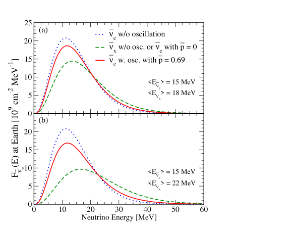
Figure 5: The expected neutrino flux spectra at the Earth for a SN located at 10 kpc from the Earth. To calculate SN neutrino flux at the Earth, we assumed that at the SN neutrinosphere, $\langle E_{\bar{\nu}_{e}}\rangle$ = 15 MeV (dotted blue curves) whereas $\langle E_{\nu_{x}}\rangle$ = 18 MeV and 22 MeV for the upper and lower panel, respectively (dashed green curves). For both cases, we show the expected $\bar{\nu}_{e}$ flux at the Earth by the solid red curves, given by Eq. (5). For simplicity, we consider that only the standard MSW effect plays a role in oscillations so that $\bar{p}=$ 0.69 (0) corresponds to the normal (inverted) mass hierarchy.

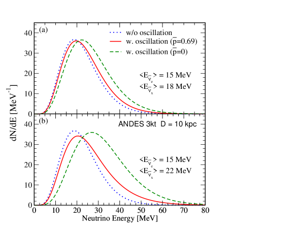
Figure 6: Expected energy distribution of $\bar{\nu}_{e}$ events coming from a SN located at 10 kpc from the Earth at the ANDES 3 kt detector. We assumed that at the SN neutrinosphere, $\langle E_{\bar{\nu}_{e}}\rangle$ = 15 MeV (dotted blue curves) whereas $\langle E_{\nu_{x}}\rangle$ = 18 MeV and 22 MeV for the upper and lower panels, respectively (dashed green curves). For both cases, we show the expected $\bar{\nu}_{e}$ flux at the Earth for the normal (inverted) mass hierarchy by the solid (dashed) red curves.

III.2 Inverse beta decay reaction

In this paper, we focus on two main reactions. One is the inverse beta decay $\bar{\nu}_{e}+p\to n+e^{+}$, which is the predominant channel due to its larger cross section, and the other is the proton-neutrino elastic scattering, $\nu+p\to\nu+p$, which is useful to determine the original $\nu_{x}$ spectra Beacom:2002hs ; Dasgupta:2011wg . Based on the fluxes shown in Fig. 5, we present in Table 4 the expected number of events we have computed for the ANDES neutrino detector in the absence and presence of neutrino oscillations, for normal and inverted mass hierarchy and different $\langle E_{\nu_{x}}\rangle$.

Only for Table 4, for the purpose of comparison, we have considered three different chemical compositions for the liquid scintilator. These are mixtures that are already used by the existing or planned detectors, KamLAND KamLAND , Borexino Alimonti:2000xc and SNO+ Kraus:2010zzb . KamLAND is based on the mixture of 80% of C₁₂H₂₆ and 20% of C₉H₁₂, whereas Borexino and SNO+ are based on C₉H₁₂ (pseudocumene) and C₆H₅C₁₂H₂₅ (alkyl benzene), respectively. For the rest of the paper we assume the same composition of SNO+.

Regarding the oscillation probabilities, it is sufficient at this point to consider the two extreme cases of the standard scenario where $\bar{p}=0.69$ and $\bar{p}=0$ corresponding, respectively, to the normal and inverted mass hierarchy. As mentioned before, apart from some possible non-trivial energy dependence, one expects the actual number of events to lay between these two cases even if other oscillation effects come into play.

	Chemical Composition of the Scintillator
Reaction	(a) C12H26 + C9H12	(b) C9H12	(c) C6H5C12H25	Assumptions
	( 80% + 20% )	pseudocumene	alkyl benzene
$\bar{\nu}_{e}+p\to n+e^{+}$	873	630	762	No Oscillation
$\bar{\nu}_{e}+p\to n+e^{+}$	924	669	804	$\bar{p}=c_{12}^{2}$ = 0.69 (NH), $\langle E_{\nu_{x}}\rangle$= 18 MeV
$\bar{\nu}_{e}+p\to n+e^{+}$	1038	750	903	$\bar{p}$ = 0.0 (IH),   $\langle E_{\nu_{x}}\rangle$= 18 MeV
$\bar{\nu}_{e}+p\to n+e^{+}$	957	690	834	$\bar{p}=c_{12}^{2}$ = 0.69 (NH), $\langle E_{\nu_{x}}\rangle$= 20 MeV
$\bar{\nu}_{e}+p\to n+e^{+}$	1140	825	993	$\bar{p}$ = 0.0 (IH),   $\langle E_{\nu_{x}}\rangle$= 20 MeV
$\bar{\nu}_{e}+p\to n+e^{+}$	987	714	858	$\bar{p}=c_{12}^{2}$ = 0.69 (NH), $\langle E_{\nu_{x}}\rangle$= 22 MeV
$\bar{\nu}_{e}+p\to n+e^{+}$	1239	894	1080	$\bar{p}$ = 0.0 (IH),   $\langle E_{\nu_{x}}\rangle$= 22 MeV
$\nu+p\to\nu+p$	294	318	453	all flavors  $T_{\text{que}}>0.2$ MeV, $\langle E_{\nu_{x}}\rangle$= 18 MeV
$\nu+p\to\nu+p$	399	405	561	all flavors  $T_{\text{que}}>0.2$ MeV,  $\langle E_{\nu_{x}}\rangle$= 20 MeV
$\nu+p\to\nu+p$	510	492	663	all flavors  $T_{\text{que}}>0.2$ MeV,  $\langle E_{\nu_{x}}\rangle$= 22 MeV

Table 4: Expected number of SN neutrino induced events for the inverse beta decay and proton-neutrino elastic scattering for the 3 types of liquid scintillators with the fiducial mass of 3 kt for a SN at 10 kpc from the Earth. They are (a) 80% of C₁₂H₂₆ and 20% of C₉H₁₂ used for KamLAND, (b) C₉H₁₂ (pseudocumene) used for Borexino, and (c) C₆H₅C₁₂H₂₅ (alkyl benzene) to be used for SNO+. NH and IH indicate the normal and inverted mass hierarchies, respectively. For $\nu+p\to\nu+p$, we considered the kinetic (quenched) energy of the recoil proton, $T_{\text{que}}$, larger than 0.2 MeV following Refs. Beacom:2002hs ; Dasgupta:2011wg .

In Fig. 6 we show the expected $\bar{\nu}_{e}$ event number distribution $dN/dE$ for our reference ANDES neutrino detector in the absence and presence of neutrino oscillations. Depending on the oscillation probabilities, we expect to have $\sim 800-1000$ events for 3 kt (see Table 4). In the presence of oscillation, the energy spectrum of $\bar{\nu}_{e}$ gets harder whereas its total flux will decrease, as we assume that the original value of $\Phi_{\nu_{\alpha}}\langle E_{\nu_{\alpha}}\rangle$ is constant for all 6 species. Nevertheless, the oscillation effect makes the expected observed event number larger, as the cross section depends on $\sim E_{\nu}^{2}$, which overcomes the reduction of the flux due to oscillations.

Due to neutrino oscillations the observed spectra at the Earth is, in general, a mixture of the original ones it would be desirable to be able to reconstruct the original spectra from data.

In principle, by fitting the observed positron spectrum of $\bar{\nu}_{e}$ induced events at the detector, one can try to reconstruct the original spectra (luminosites and average energies) of $\bar{\nu}_{e}$ and $\bar{\nu}_{x}$ as done, for example, in Refs. Minakata:2001cd ; Skadhauge:2006su but in practice, this may not be so trivial to do, even for a much larger detector such as Hyper-Kamiokande Abe:2011ts , due to the possible presence of degeneracies of the SN parameters Minakata:2008nc or some unexpected large deviation of SN neutrino spectra from what is usually assumed.

As far as the reconstruction of the spectra of $\bar{\nu}_{x}$ is concerned, the use of the proton-neutrino elastic scattering seems to be more promising Beacom:2002hs ; Dasgupta:2011wg . This will be discussed in the next subsection. We propose to combine both, the inverse beta decay and proton-neutrino reactions, in order to identify the oscillation effect, or determine SN parameters if oscillation effect is known, as we will discuss in subsection III.4.

III.3 Proton-neutrino elastic scattering

In this section, we focus on the proton-neutrino elastic scattering discussed in Refs. Beacom:2002hs ; Dasgupta:2011wg ; Wurm:2011zn . Since the proton-neutrino elastic scattering, $\nu+p\to\nu+p$, for all flavors, occurs via neutral current interactions, one can measure the total SN neutrino flux above a certain energy threshold, without worrying about any oscillation effect among active flavors, in a similar manner as the SNO experiment was able to measure the total solar neutrino flux of active flavors Ahmad:2002jz . If the average energies of $\nu_{e}$ and $\bar{\nu}_{e}$ are significantly lower than that of $\nu_{x}$, then by counting the total number of events above a certain recoil proton energy, one can measure the total flux (luminosity) of $\nu_{x}$ flavor with reasonably good precision Beacom:2002hs ; Dasgupta:2011wg . If the energy spectra of SN $\nu_{e}$, $\bar{\nu}_{e}$, and $\nu_{x}$ are rather similar, one can then try to determine the total neutrino flux.

To compute the number of events induced by the $\nu$-$p$ elastic scattering, we follow the analysis procedure described in Refs. Beacom:2002hs ; Dasgupta:2011wg . We have checked that by using the same information and assumption used in these references we could obtain results which are in good agreement with the ones presented in these works.

In Fig. 7 we show the expected event number distribution, $dN/dT_{\text{que}}$, as a function of the quenched kinetic proton energy, $T_{\text{que}}$, for the ANDES reference neutrino detector and for the reference SN parameters summarized in Table 3.

Figure 7: Distribution of events as a function of the quenched kinetic energy of the proton for the ANDES reference detector using the reference SN parameters defined in Table 3.

Following Dasgupta:2011wg , the energy range of $T_{\text{que}}>0.2$ MeV was considered mainly because of the backgrounds coming from radioactive decays in the scintillator and surroundings, such as the one coming from the $\beta$ decay of ¹⁴C. The qualitative behavior of $dN/dT_{\text{que}}$ for the ANDES detector is very similar to the ones obtained in Dasgupta:2011wg for KamLAND, Borexino and SNO+ detectors (see Figs. 1-3 of this reference), the main difference is the total number of events.

We have studied how accurately one can reconstruct the original neutrino flux by the energy distribution of recoil protons in the ANDES detector. As demonstrated explicitly in Ref. Dasgupta:2011wg by considering the quenched proton recoil energy larger than 0.2 MeV, one can reconstruct the original neutrino flux above $\;>$$\sim\;$ 25 MeV. The idea is to make an inversion of the calculation in order to produce the curves shown in Fig. 7.

In Fig. 8 we show our result. For our reference SN, with the 3 kt ANDES detector, one can try to determine the original neutrino flux with the precision of $\sim$ 15 % for the neutrino energy $\sim$ 20-40 MeV. Note that this result does not depend on the uncertainty on the effects of neutrino oscillations among active flavors, which could occur in the SN envelope. While the expected precision is not as good as the one expected for the proposed much larger LENA detector Wurm:2011zn , which has 50 kt fiducial volume, as we can compare our results with the one shown in Fig. 9 of Ref. Dasgupta:2011wg , the expected precision for the ANDES detector is better than the currently existing (planned) detectors like KamLAND and Borexino (SNO+).

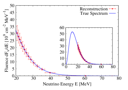
Figure 8: Reconstruction of the original SN neutrino flux (indicated by the red solid circles with error bar of 1 $\sigma$), from the simulated future data of proton-neutrino elastic scattering in the ANDES detector under the same assumptions used in Fig. 7, for the reference SN parameters defined in Table 3.

Next let us discuss with which precision we can try to determine the original $\nu_{x}$ mean energy. For this purpose, we perform a $\chi^{2}$ analysis by considering the input (true) values of SN parameters for $\langle E_{\nu_{x}}\rangle$ = 15, 18 and 22 MeV and $E^{\text{tot}}_{\nu_{x}}=5\times 10^{52}$ erg. We define $E^{\text{tot}}_{\nu_{x}}$ such that 4$E^{\text{tot}}_{\nu_{x}}$ gives the total energy carried away by non-electron flavor neutrinos. For simplicity, we fix the other SN parameters for $\nu_{e}$ and $\bar{\nu}_{e}$ to our reference values, and only vary $E^{\text{tot}}_{\nu_{x}}$ and $\langle E_{\nu_{x}}\rangle$ in our fit, in order to have some feeling about the precision we can achieve. We show our result in Fig. 9 where the allowed parameter regions in the plane of $E^{\text{tot}}_{\nu_{x}}$ and $\langle E_{\nu_{x}}\rangle$ is shown. Here only the statistical uncertainties were taken into account. From this, we conclude that we can determine $\langle E_{\nu_{x}}\rangle$ and $E^{\text{tot}}_{\nu_{x}}$ with the precisions of $\sim 6$% (25%) and $\sim 20$% (40%), respectively, at 1 (3) $\sigma$ CL, for the case where the true values of $\langle E_{\nu_{x}}\rangle$ and $E^{\text{tot}}_{\nu_{x}}$ were assumed to be 18 MeV and $5\times 10^{52}$ erg, respectively.

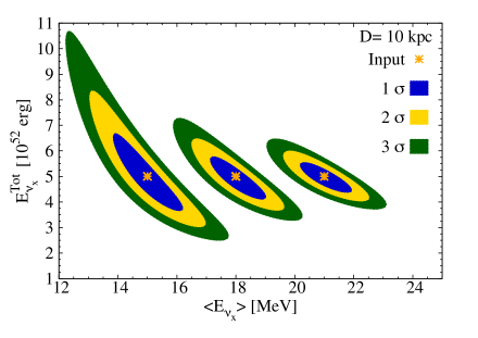
Figure 9: Sensitivity of the determination of the original $E^{\text{tot}}_{\nu_{x}}$ and $\langle E_{\nu_{x}}\rangle$ at 1,2 and 3 $\sigma$ CL, by proton-neutrino scattering events measured at the ANDES detector. Only the statistical uncertainties were taken into account. We consider three different input values for the average $\bar{\nu}_{x}$ energy, $\langle E_{\nu_{x}}\rangle$ = 15 MeV, 18 MeV and 21 MeV while that for $E^{\text{tot}}_{\nu_{x}}$ was fixed to be $5\times 10^{52}$ erg (they are indicated by the asterisk). The other SN parameters are defined in Table 3.

III.4 Comparison of CC and NC induced events

As mentioned in the previous subsection, one of the important features of the reaction induced by proton neutrino elastic scattering is that it does not depend on the neutrino oscillation among active flavors, as this reaction is induced by neutral current (NC). On the other hand, the inverse beta decay is induced by charged current (CC) interactions and so does depend on the neutrino oscillation probability, as can be seen in Table 4.

Therefore, by comparing these two kinds of events, one can try to infer, to some extent, the oscillation effect or the value of $\bar{p}$ in Eq.(4) in a less model dependent way. Or conversely, if the mass hierarchy is known (from some other source, like one of the long-baseline neutrino oscillation experiments) by the time the next galactic SN occurs, and $\bar{p}$ can be predicted in advance, one can try to determine better some other characteristic of the SN neutrinos. We observe that the comparison of CC and NC events was also considered in Borexino-SN-nu .

For the purpose of illustration, let us define the following ratio,

$$R(N_{\bar{\nu}_{e}p}/N_{\nu p})\equiv\displaystyle\left(\frac{N_{\bar{\nu}_{e}p}}{N_{\nu p}}\right)^{\text{obs}},$$ (6)

where $(N_{\bar{\nu}_{e}p}/N_{\nu p})^{\text{obs}}$ means the ratio of the observed total number of events induced by the inverse beta decay and proton-neutrino elastic scattering.

In Fig. 10 we show this quantity as a function of the true value of $\langle E_{\nu_{x}}\rangle$. For $\bar{p}$, we considered the two extreme values of the standard scenario, $\bar{p}$ = 0 and 0.69. For this study, we consider the two cases where $D=$ 5 and 10 kpc, indicated by the darker and lighter color, respectively.

We note that if $\langle E_{\nu_{x}}\rangle$ is significantly different from $\langle E_{\bar{\nu}_{e}}\rangle$, one can try to identify the presence of oscillation effect by inferring the value of $\bar{p}$ with some precision, which could be possible especially for the case where the true value of $\langle E_{{\nu}_{x}}\rangle$ turns out to be quite different from $\langle E_{\bar{\nu}_{e}}\rangle$. This may be the case during the accretion phase as energies and luminosities of $\bar{\nu}_{e}$ and $\nu_{x}$ may be significantly different, as recent SN simulations indicate Fischer:2009af ; Huedepohl:2009wh ; Fischer:2011cy . Moreover, in this phase, as mentioned before recent studies Chakraborty:2011nf ; Sarikas:2011am indicate that the collective effects could be suppressed by matter, which means that the neutrino conversion would be given by the standard scenario. This would allows us to identify the oscillation effect more easily, provided that the number of events for this phase is large enough.

However, it must be stressed that differences or similarities between $\bar{\nu}_{e}$ and $\nu_{x}$ fluxes must be confirmed (or refuted) by observations. The real SN neutrino data could be very different from our expectations! We also should keep in mind that the characteristics of SN neutrinos may depend strongly on the SN (on the progenitor’s mass, chemical composition of the core, etc.) (see e.g., Lunardini:2007vn ).

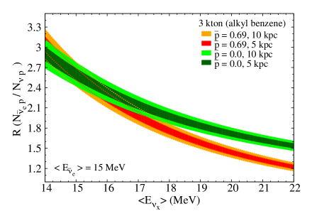
Figure 10: The ratio, $R(N_{\bar{\nu}_{e}p}/N_{\nu p})$, as a function of the true value of $\langle E_{\nu_{x}}\rangle$ for our reference ANDES neutrino detector. The values of the SN parameters not specified in this plot are the ones defined in Table 3.

In Fig. 11 we show the same quantity, $R(N_{\bar{\nu}_{e}p}/N_{\nu p})$, but as a function of the true (input) value of $\langle E_{\bar{\nu}_{e}}\rangle$ for the cases where the true value of $\langle E_{\nu_{x}}\rangle$ is 18 MeV. A similar conclusion can be drawn as before. Unless $\langle E_{\bar{\nu}_{e}}\rangle$ is significantly different from $\langle E_{\nu_{x}}\rangle$, it will not be very easy to distinguish $\bar{p}=0$ from $\bar{p}=0.69$. We can also use these results to do the opposite. Namely, if we know the mass hierarchy by the time of the next galactic SN observation, we can try to infer, to some extent, the original values of $\langle E_{\bar{\nu}_{e}}\rangle$ and $\langle E_{\nu_{x}}\rangle$ from data.

In Fig. 12 we show $R(N_{\bar{\nu}_{e}p}/N_{\nu p})$ as a function of $\bar{p}$ for the cases where the true values of $\langle E_{\nu_{x}}\rangle$ are 18 and 21 MeV. We see again that unless $\langle E_{\nu_{x}}\rangle$ is significantly different from $\langle E_{\bar{\nu}_{e}}\rangle$, it is not easy to identify the oscillation effect, especially if the hierarchy is normal and $\bar{p}$ = 0.69. The case of inverted hierarchy, $\bar{p}$ = 0.0, seems easier to be identified.

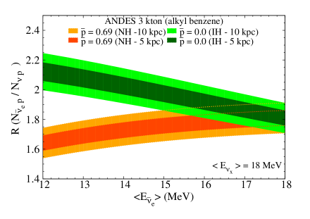
Figure 11: Same as Fig. 10 but as a function of the true value of $\langle E_{\bar{\nu}_{e}}\rangle$. The values of the SN parameters not specified in this plot are the ones defined in Table 3.

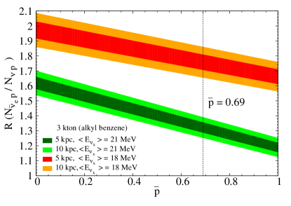
Figure 12: Same as Fig. 10 but as a function of $\bar{p}$ for the cases where the true value of $\langle E_{\nu_{x}}\rangle$ = 18 and 21 MeV.

In Fig. 13 we show the ratio $R(N_{\bar{\nu}_{e}p}/N_{\nu p})$ as a function of $L_{\bar{\nu}}/L_{\nu_{x}}\equiv(\langle E_{\bar{\nu}_{e}}\rangle\Phi_{\bar{\nu}_{e}})/(\langle E_{{\nu}_{x}}\rangle\Phi_{{\nu}_{x}})$ for the case where the true value of $\langle E_{\nu_{x}}\rangle$ is 18 MeV. This plots indicate that if the luminosity of $\bar{\nu}_{e}$ is larger than that of $\nu_{x}$ by $\sim 20$ % or so, the cases of normal and inverted mass hierarchy can be confused. However, if $\bar{\nu}_{e}$ luminosity is significantly larger or smaller (by $\sim 50$ % or more), then it is easier to distinguish the mass hierarchy. On the other hand, if the mass hierarchy is known by the time the next SN neutrinos are observed, then we can try to infer the difference of the luminosities of $\bar{\nu}_{e}$ and $\nu_{x}$.

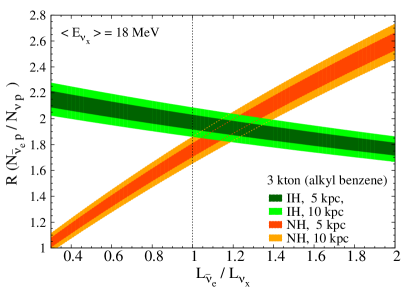
Figure 13: Same as Fig. 10 but as a function of the true value of $L_{\bar{\nu}}/L_{\nu_{x}}\equiv(\langle E_{\bar{\nu}_{e}}\rangle\Phi_{\bar{\nu}_{e}})/(\langle E_{{\nu}_{x}}\rangle\Phi_{{\nu}_{x}})$ for the cases where the true value of $\langle E_{\nu_{x}}\rangle$ = 18 MeV. The values of the SN parameters not specified in this plot are the ones defined in Table 3.

III.5 Earth Matter Effect: Shadowing Probabilities

One potentially interesting possibility is to observe the Earth matter effect due to SN neutrinos Dighe:1999bi ; Lunardini:2001pb ; Dighe:2003jg ; Dighe:2003vm . If observed, it could unravel the neutrino mass hierarchy and some properties of the SN neutrino fluxes. Suppose that SN neutrinos are observed by more than two neutrino detectors. If some of them (but not all) receive SN neutrinos passing through the Earth interior (shadowed by the Earth) but at the same time, there are some other group of detectors which receive SN neutrinos without passing through the Earth interior (non shadowed by the Earth), it would be interesting to compare the results of these two group of detectors.

Currently, several neutrino detectors, which can observe neutrinos coming from a galactic SN, are in operation. Among them we can highlight Super-Kamiokande (SK) Ikeda:2007sa , KamLAND KamLAND , Borexino Alimonti:2000xc , IceCube Abbasi:2011ss and LVD Bari:1989nw . In this paper we will consider the following laboratory sites: Kamioka (SK and KamLAND), the South Pole (IceCube), Sudbury (SNO+) Kraus:2010zzb and ANDESAndes-Website . In Table 5 we show the positions of the detectors we consider in this work.

Site	Latitude	Longitude	Shadowing Prob.
			Mantle  (Core)
Kamioka, Japan	36.42oN	137.3o E	0.559 (0.103)
South Pole	90oN	-	0.413 (0.065)
ANDES	30.25oS	68.88oW	0.449 (0.067)
SNO, Canada	46.476oN	81.20oE	0.571 (0.110)

Table 5: Positions of the detectors we consider in this paper. In the last column, we show the shadowing probability, the probability that SN neutrinos will pass only through the mantle (indicated as Mantle) or will pass both through the mantle and core (indicated as Core).

Following Ref. Mirizzi:2006xx , we have calculated the shadowing probabilities for the cases where $N$ ($N=1,2,3,4$) detectors are considered simultaneously. The shadowing probability is defined as the probability that a given detector or combination of detectors receives neutrinos from a galactic SN with Earth matter effect either by passing only through the mantle or both through the core and the mantle of the Earth Mirizzi:2006xx .

Using the same model of SN distribution in the Milky Way considered in Ref. Mirizzi:2006xx , which is based on the neutron star distribution (reproduced in Eqs. (19) and (20) of the Appendix C) we can compute the shadowing probability for an arbitrary number of detector positions on the Earth.

The shadowing probability for the most simple case where only a single detector is considered is shown in the last column of Table 5. For the case where two detector locations, Kamioka and South Pole, are considered simultaneously, we show the results in Table 6. We observe that the numbers shown in this table agree well with the ones found in Table 2 of Ref. Mirizzi:2006xx . From Table 6 we conclude that the probability that only one of these detectors observes SN neutrinos having passed through the Earth is about 72%.

	Earth Matter Effect
Case	Kamioka	South Pole	Shadowing Prob.
			Mantle  (Core)
(1)	No	No	0.152 (0.832)
(2)	Yes	No	0.435 (0.104)
(3)	No	Yes	0.288 (0.065)
(4)	Yes	Yes	0.125 (0.000)

Table 6: Earth shadowing probability for the case where two detectors at Kamioka and South Pole are considered.

	Earth Matter Effect
Case	Kamioka	South Pole	ANDES	Shadowing Prob.
				Mantle (Core)
(1)	No	No	No	0.024 (0.767)
(2)	Yes	No	No	0.388 (0.105)
(3)	No	Yes	No	0.034 (0.061)
(4)	No	No	Yes	0.128 (0.063)
(5)	Yes	Yes	No	0.106 (0.000)
(6)	No	Yes	Yes	0.254 (0.003)
(7)	Yes	No	Yes	0.047 (0.000)
(8)	Yes	Yes	Yes	0.020 (0.000)

Table 7: Earth shadowing probability for the case where detectors at Kamioka, South Pole and Andes sites are considered.

	Earth Matter Effect
Case	Kamioka	South Pole	ANDES	Sudbury	Shadowing Prob.
					Mantle (Core)
(1)	No	No	No	No	0.008 (0.657)
(2)	Yes	No	No	No	0.206 (0.105)
(3)	No	Yes	No	No	0.034 (0.061)
(4)	No	No	Yes	No	0.001 (0.063)
(5)	No	No	No	Yes	0.016 (0.111)
(6)	Yes	Yes	No	No	0.205 (0.000)
(7)	Yes	No	Yes	No	0.000 (0.000)
(8)	Yes	No	No	Yes	0.282 (0.000)
(9)	No	Yes	Yes	No	0.163 (0.003)
(10)	No	Yes	No	Yes	0.000 (0.000)
(11)	No	No	Yes	Yes	0.127 (0.000)
(12)	No	Yes	Yes	Yes	0.091 (0.000)
(13)	Yes	No	Yes	Yes	0.047 (0.000)
(14)	Yes	Yes	No	Yes	0.011 (0.000)
(15)	Yes	Yes	Yes	No	0.012 (0.000)
(16)	Yes	Yes	Yes	Yes	0.008 (0.000)

Table 8: Earth shadowing probability for the case where detectors at Kamioka, South Pole, ANDES and Sudbury sites are considered.

Next in Table 7 we show the Earth shadowing probabilities for the case where we consider three detectors: at Kamioka, South Pole and ANDES sites. From this table, we see that the probability of having at least one of these detectors observing SN neutrinos passing through the Earth while at least one of the other two sees them non shadowed by the Earth is 96%, which is about 30% larger than the case above with two detectors, one at Kamioka and the other at the South Pole. One can also compare our three detector combination with any two detector combination found in Table 2 of Ref. Mirizzi:2006xx where the largest probability for having one detector shadowed and one non shadowed is 87.2%, occurring for the Pyhäsalmi and South Pole sites.

In Table 8 we show the case where four detectors at Kamioka, South Pole, ANDES and Sudbury sites are considered. With four detectors, the probability that at least one of the detectors have the Earth effect and at least one of the others have not, increases to 98%. We also found that the probability that at least one of these sites receives a SN neutrino flux which passes the core of the Earth is not very small, $\sim$ 34%.

III.6 Quantifying the Earth matter effect: Comparing the detectors with and without Earth matter effect

Let us now try to quantify the Earth matter effect which could be observed in a model independent way by comparing the yields of two (or more) detectors if only some (not all) of them receive SN neutrinos passing through the Earth’s interior. See  Dighe:1999bi ; Lunardini:2001pb ; Dighe:2003jg ; Dighe:2003vm for the previous works.

In this paper, we focus on the possible Earth matter effect for $\bar{\nu}_{e}$ due to the larger number of expected events. Since we know now that $\theta_{13}$ is not too small, $\sin^{2}2\theta_{13}\simeq 0.09-0.1$ Abe:2011sj ; Adamson:2011qu ; Abe:2011fz ; An:2012eh ; collaboration:2012nd , it is expected that Earth matter effect can only be large for the normal mass hierarchy in the standard scenario we consider in this work Dighe:1999bi . So we will assume here only the normal hierarchy in such a standard scenario. Note that for the case of $\bar{\nu}_{e}$ in the normal mass hierarchy, collective effects, shock wave, etc. are in general expected to be small.

If SN neutrinos reach the detector after passing through the Earth matter, assuming the impact of non-zero $\theta_{13}$ is not very significant for the Earth matter effect itself (though the impact of $\theta_{13}$ is expected to be large for the oscillations inside the SN, affecting significantly $\bar{p}(E)$ especially for the case of the inverted mass hierarchy), the SN flux spectrum is expected to get modified as follows Dighe:1999bi ,

$$F_{\bar{\nu}_{e}}^{\oplus}(E)=\bar{p}^{\oplus}(E)F_{\bar{\nu}_{e}}^{0}(E)+[1-\bar{p}^{\oplus}(E)]F_{\bar{\nu}_{x}}^{0}(E),$$ (7)

where

$$\bar{p}^{\oplus}(E)=\frac{1}{|U_{e2}|^{2}-|U_{e1}|^{2}}\left[\left\{|U_{e2}|^{2}-\bar{p}(E)\right\}\bar{p}^{\oplus}_{1e}+\left\{\bar{p}(E)-|U_{e1}|^{2}\right\}\bar{p}^{\oplus}_{2e}\right],$$ (8)

where $U_{ek}$ ($k=1,2$) are the elements of neutrino mixing matrix which relate flavor and mass eigenstates and

$$\bar{p}^{\oplus}_{ke}\equiv P^{\oplus}(\bar{\nu}_{k}\to\bar{\nu}_{e},L),\ \ (k=1,2),$$ (9)

are the probabilities that a mass eigenstate $\bar{\nu}_{k}$ $(k=1,2)$ entering the Earth will be detected as $\bar{\nu}_{e}$ at the detector, after traveling the distance $L$ inside the Earth.

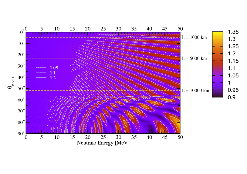
Figure 14: Neutrino Oscillogram, iso-contour plot of the ratio $P^{\oplus}(\bar{\nu}_{1}\to\bar{\nu}_{e})/c_{12}^{2}$ in the plane of the neutrino energy and the nadir angle. Note that unity for this ratio corresponds to the case where the Earth matter effect is absent.

If we take the difference of SN spectra given in Eqs. (7) and (4) with and without Earth matter effect,

$$\Delta F_{\bar{\nu}_{e}} \equiv F_{\bar{\nu}_{e}}^{\oplus}(E)-F_{\bar{\nu}_{e}}(E)$$ (10)

$$= \frac{1}{|U_{e1}|^{2}-|U_{e2}|^{2}}\left\{[2\bar{p}(E)-1]\left(|U_{e2}|^{2}-\bar{p}^{\oplus}_{2e}\right)+|U_{e3}|^{2}\left(\bar{p}(E)-\bar{p}^{\oplus}_{2e}\right)\right\}\left\{F_{\bar{\nu}_{e}}^{0}(E)-F_{\bar{\nu}_{x}}^{0}(E)\right\}$$

$$\simeq \frac{1}{\cos 2\theta_{12}}[2\bar{p}(E)-1](s^{2}_{12}-\bar{p}^{\oplus}_{2e})\left\{F_{\bar{\nu}_{e}}^{0}(E)-F_{\bar{\nu}_{x}}^{0}(E)\right\}$$

$$\simeq (\bar{p}^{\oplus}_{1e}-c^{2}_{12})\left\{F_{\bar{\nu}_{e}}^{0}(E)-F_{\bar{\nu}_{x}}^{0}(E)\right\},$$

where $\bar{p}(E)\approx c_{12}^{2}$ was assumed to get the last expression. We also observe that the term proportional to $|U_{e3}|^{2}$ can be dropped because it will only contribute to about 7% of the first term. As one can see from Eq. (10), in order to observe the Earth matter effect, the deviation of $\bar{p}^{\oplus}_{1e}$ from $c^{2}_{12}$ must be large enough and at the same time, the difference between the original spectra of $F_{\bar{\nu}_{e}}^{0}(E)$ and $F_{\bar{\nu}_{x}}^{0}(E)$ must be also significantly large.

In order to have some idea about the magnitude of the Earth matter effect as functions of the neutrino energy and the incident angle of SN neutrinos, we show in Fig. 14 the iso-contours of the quantity $P^{\oplus}(\bar{\nu}_{1}\to\bar{\nu}_{e})/c_{12}^{2}$ in the plane of the nadir angle, $\theta_{\text{nadir}}$, and the neutrino energy where $P^{\oplus}(\bar{\nu}_{1}\to\bar{\nu}_{e})$ was obtained by numerically integrating the neutrino evolution equation using the matter density profile of the Earth based on PREM (Preliminary Reference Earth Model) Dziewonski:1981xy . Note that any deviation of $P^{\oplus}(\bar{\nu}_{1}\to\bar{\nu}_{e})/c_{12}^{2}$ from unity implies the presence of the Earth matter effect.

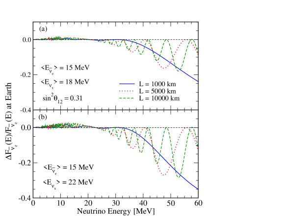
Figure 15: The fractional difference of the expected neutrino flux spectra with and without the Earth matter effect, $\Delta F_{\bar{\nu}_{e}}/F_{\bar{\nu}_{e}}$ where $\Delta F_{\bar{\nu}_{e}}\equiv F_{\bar{\nu}_{e}}^{\oplus}(E)-F_{\bar{\nu}_{e}}(E)$, given in Eq. (10). The SN neutrino parameters are the same as assumed in Fig. 5.

This plot is similar to the so called “neutrino oscillogram” studied in detail in Ref. nu-oscillogram in the context of atmospheric neutrinos. As we can see from this plot, the Earth effect is as expected strongest when neutrinos pass through the Earth’s core (corresponding to $\theta_{\text{nadir}}\raise 1.29167pt\hbox{$\;<$\kern-7.5pt\raise-4.73611pt\hbox{$\sim\;$}}33^{\circ}$) and for higher neutrino energies. Here $\theta_{\text{nadir}}$ is defined such that $\theta_{\text{nadir}}=0^{\circ}$ corresponds to the case where SN neutrinos arrive at the detector from the other side of the Earth passing the center of the Earth and $\theta_{\text{nadir}}=90^{\circ}$ corresponds to the case where neutrinos come from the horizontal direction.

In Fig. 15 we show the fractional difference of the flux spectra with and without the Earth effect defined by $\Delta F_{\bar{\nu}_{e}}/F_{\bar{\nu}_{e}}$ where $\Delta F_{\bar{\nu}_{e}}$ is given by Eq. (10) for for three different path-lengths in the Earth, $L=1000$ km (solid blue curve), $L=5000$ km (dotted red curve) and $L=10000$ km (dashed green curve). From this figure, we can see that strong Earth matter effect is expected in the higher energy range. We must note, however, that as the energy becomes higher, the number of events gets smaller, so that in order to identify the Earth matter effect, both the Earth effect (difference of probabilities with and without matter effect) and the number of events in the relevant energy range must be large enough.

	$~{}E<30$ MeV	$~{}30<E/{\rm MeV}<40~{}$	$~{}40<E/{\rm MeV}<50~{}$	$~{}E>50$ MeV	Case	Compatibility
Vacuum (observed)	18159 $\pm$ 135	4973 $\pm$ 71	2032 $\pm$ 45	889 $\pm$ 30	$\langle E_{\nu_{x}}\rangle$ = 22 MeV	$3.1\sigma$
1000 km (prediction)	18132 $\pm$ 374	5065 $\pm$ 198	1908 $\pm$ 121	700 $\pm$ 74	$\beta_{x}=\beta_{e}=4$
Vacuum (observed)	17395 $\pm$ 132	5785 $\pm$ 76	2583 $\pm$ 51	1147 $\pm$ 34	$\langle E_{\nu_{x}}\rangle$ = 22 MeV	$2.2\sigma$
1000 km (prediction)	17370 $\pm$ 367	5858 $\pm$ 213	2483 $\pm$ 139	988 $\pm$ 87	$\beta_{x}=4$ $\beta_{e}=3$
Vacuum (observed)	16031 $\pm$ 127	6674 $\pm$ 82	3594 $\pm$ 60	1978 $\pm$ 45	$\langle E_{\nu_{x}}\rangle$ = 22 MeV	$0.7\sigma$
1000 km (prediction)	16011 $\pm$ 352	6728 $\pm$ 228	3541 $\pm$ 166	1917 $\pm$ 122	$\beta_{x}=4$ $\beta_{e}=2$
Vacuum (observed)	16863 $\pm$ 130	5722 $\pm$ 76	2864 $\pm$ 54	1604 $\pm$ 40	$\langle E_{\nu_{x}}\rangle$ = 22 MeV	$3.2\sigma$
1000 km (prediction)	16837 $\pm$ 361	5787 $\pm$ 212	2731 $\pm$ 145	1321 $\pm$ 101	$\beta_{x}=\beta_{e}=3$
Vacuum (observed)	15499 $\pm$ 125	6611 $\pm$ 81	3875 $\pm$ 62	2434 $\pm$ 49	$\langle E_{\nu_{x}}\rangle$ = 22 MeV	$1.7\sigma$
1000 km (prediction)	15479 $\pm$ 346	6657 $\pm$ 227	3789 $\pm$ 171	2250 $\pm$ 132	$\beta_{x}=3$ $\beta_{e}=2$
Vacuum (observed)	14790$\pm$122	6388$\pm$ 80	4089$\pm$ 64	3059$\pm$ 55	$\langle E_{\nu_{x}}\rangle$ = 22 MeV	$2.8\sigma$
1000 km (prediction)	14766$\pm$338	6419$\pm$223	3971$\pm$ 175	2701$\pm$ 145	$\beta_{x}=\beta_{e}=2$
Vacuum (observed)	17686$\pm$133	5240$\pm$72	2439$\pm$49	1285 $\pm$36	$\langle E_{\nu_{x}}\rangle$ = 24 MeV	$4.3\sigma$
1000 km (prediction)	17655$\pm$370	5343$\pm$203	2272$\pm$133	990$\pm$88	$\beta_{x}=\beta_{e}=4$
Vacuum (observed)	16922$\pm$130	6052$\pm$78	2990$\pm$55	1543$\pm$39	$\langle E_{\nu_{x}}\rangle$ = 24 MeV	$3.1\sigma$
1000 km (prediction)	16892$\pm$362	6136$\pm$218	2847$\pm$ 148	1278$\pm$100	$\beta_{x}=4$ $\beta_{e}=3$
Vacuum (observed)	15557$\pm$125	6941$\pm$83	4001$\pm$63	2374$\pm$49	$\langle E_{\nu_{x}}\rangle$ = 24 MeV	$1.7\sigma$
1000 km (prediction)	15533$\pm$347	7006$\pm$233	3905$\pm$174	2207$\pm$ 131	$\beta_{x}=4$ $\beta_{e}=2$
Vacuum(observed)	16441$\pm$128	5858$\pm$77	3174$\pm$56	2022$\pm$45	$\langle E_{\nu_{x}}\rangle$ = 24 MeV	$4.0\sigma$
1000 km (prediction)	16409 $\pm$356	5928$\pm$214	3007$\pm$ 153	1625$\pm$112	$\beta_{x}=\beta_{e}=3$
Vacuum (observed)	15077$\pm$123	6746$\pm$82	4185$\pm$65	2853$\pm$53	$\langle E_{\nu_{x}}\rangle$ = 24 MeV	$2.5\sigma$
1000 km (prediction)	15051$\pm$341	6797$\pm$229	4065$\pm$177	2554$\pm$141	$\beta_{x}=3$ $\beta_{e}=2$
Vacuum (observed)	14439$\pm$120	6400$\pm$80	4248$\pm$65	3402$\pm$58	$\langle E_{\nu_{x}}\rangle$ = 24 MeV	$3.3\sigma$
1000 km (prediction)	14410$\pm$334	6430$\pm$223	4116$\pm$179	2948$\pm$151	$\beta_{x}=\beta_{e}=2$

Table 9: Number of inverse $\beta$-decay events expected at the SK detector (1.7 $\times 10^{33}$ free protons) for a SN happening at 5 kpc from the Earth for $E<30$ MeV, $30<E/{\rm MeV}<40$, $40<E/{\rm MeV}<50$ and $E>50$ MeV for the case of vacuum and matter effect with a baseline of 1000 km and various SN parameters. We assume $L_{{\bar{\nu_{e}}}}/L_{\nu_{x}}=1$ and $\langle E_{\bar{\nu}_{e}}\rangle$ = 15 MeV. We assume that the SK detector receives SN neutrinos without the Earth matter effect whereas the ANDES neutrino detector receives them after traveling 1000 km inside the Earth. The numbers in the row indicated as vacuum are the ones to be observed at SK detector which must be compared with the theoretical prediction at SK inferred from the observed number of events at ANDES neutrino detector. In the last column we point out in how many $\sigma$ the 1000 km observation is distinguishable from vacuum.

Since we cannot compare the number of events at the same detector with and without Earth matter effect, we need two or more detectors to be able to conclude something on the matter effect. For simplicity and for the sake of discussion, let us consider only two detectors at two different sites, say, one at Kamioka (SK) and other at ANDES.

Suppose that the arrival of the SN neutrinos at the ANDES detector is shadowed by the Earth, while at SK detector at Kamioka is not. Then, to some extent, within the statistical and systematic errors, one can try to infer the expected SN spectra at SK from the observed ones at ANDES (or vice versa) as if the SK detector were also shadowed like ANDES. If both detectors receives SN neutrinos without Earth matter effect these two spectra must agree with each other but with the matter effect, they are not expected to coincide exactly.

In order to see the presence of Earth matter effect, the combination of SK and ANDES must be able to distinguish, for a given SN model, vacuum from matter event distribution. To illustrate that, we show in Table 9 the expected number of events in SK for four different energy bins for vacuum and matter with $L=1000$ km, for a variety of SN parameters. If we assume that the shadowed SN neutrino spectra distribution of events at SK can be provided by ANDES with an uncertainty in each bin equal to the statistical uncertainty in ANDES we can estimate in which of these cases one can establish the presence of matter effects. In fact, since the first bin $E<$ 30 MeV is not sensitive to matter effects, one can use it as a control bin to evaluate the accuracy of the vacuum distribution provided by ANDES data. For this study, we consider SN event at 5 kpc from the Earth as we need larger number of events for ANDES.

To give a quantitative idea of the discrimination power, we have assumed, for each SN model in Table 9 the vacuum distribution to be the hypothesis to be tested with data at 1000 km. We use the last two energy bins in order to estimate the deviation from vacuum in terms of standard deviations. These numbers are given in the last column of Table 9. For most cases, matter effects can be established in more than 2 $\sigma$. We have also verified that if $\langle E_{\nu_{x}}\rangle\raise 1.29167pt\hbox{$\;<$\kern-7.5pt\raise-4.73611pt\hbox{$\sim\;$}}18$ MeV we cannot distinguish matter effects for any value of the other SN parameters considered in Table 9, at least if $L_{{\bar{\nu_{e}}}}/L_{\nu_{x}}=1$.

IV Discussions and Conclusions

The ANDES laboratory, if constructed, will be the first deep underground laboratory in the Southern Hemisphere. It can offer the possibility to explore rare physics events that can profit from the low natural background environment because of the overburden of $\sim 4.5$ kmwe. In particular, dedicated neutrino physics and dark matter search programs, that could also benefit from the its unique geographic location, could be envisaged. See Andes-Website for updates on the status of the laboratory.

In this work, we have studied the potential of a few kt liquid scintillator neutrino detector at the ANDES underground laboratory for neutrino astrophysics and geophysics. Since there are very few nuclear reactors in South America, the location of the ANDES laboratory is specially suitable for geoneutrino observations. Moreover, due to thick continental crust around the laboratory, higher geoneutrino event rate is expected, substantially larger than at Kamioka and Gran Sasso, which by itself would be interesting to confirm experimentally.

Concerning the observations of neutrinos coming from SN, the ANDES neutrino detector could play an important role. First of all, because of the small event rate of the nearby SN (within a few 10 kpc from the Earth or so), having as many large neutrino detectors as possible is highly desirable. Furthermore, because of the location, the presence of the ANDES detector will increase the chance of observing the Earth matter effect by combining the signal at the ANDES with other detectors in the Northern Hemisphere. The ANDES neutrino detector could also integrate the international SN watch network SNEWS Antonioli:2004zb .

We have focused here on galactic SN neutrinos and geoneutrinos. However, with such a liquid scintillator detector one could also try to study solar neutrinos in a similar fashion as Borexino Borexino-solar and KamLAND Abe:2011em have done and as SNO+ Kraus:2010zzb plans to do. In fact, Borexino has shown how pep, CNO and perhaps even pp solar neutrinos can be accessible by such a detector. There is also an interesting proposal to search for indirect dark matter signals through neutrinos which are coming from the dark matter annihilation in the Sun in these type of detectors (see e.g. Kumar:2011hi ).

Appendix A Calculations of the number of event induced by the inverse beta decay reaction

The number of event induced by the inverse beta decay reaction $\bar{\nu}_{e}+p\to n+e^{+}$, is given by

$$N=N_{p}\int_{E_{\text{min}}}^{\infty}dE\ F_{\bar{\nu}_{e}}(E)\sigma_{\bar{\nu}_{e}p}(E)$$ (11)

where $E_{\text{min}}=1.806$ MeV is the threshold of this reaction, $N_{p}$ is the number of free protons in the detector and $E$ is the observed energy. For simplicity, we assume perfect energy resolution, which is a good approximation for the results presented in this work. While the accurate absorption cross section of $\bar{\nu}_{e}$ on proton, $\sigma_{\bar{\nu}_{e}p}(E)$, can be found in Ref. Strumia:2003zx , we only quote the simple approximate analytic expression given in this reference, which is sufficient for our purpose,

$$\sigma_{\bar{\nu}_{e}p}(E) \approx p_{e}E_{e}E^{-0.07056+0.02018\ln E-0.001953\ln^{3}E}$$ (12)

$$\times 10^{-43}\ \ [\text{cm}^{2}],$$

where $E_{e}=E-(m_{n}-m_{p})\simeq E-1.293$ MeV ($m_{n}$, $m_{p}$ are mass of neutron and proton, respectively), and $p_{e}$ is the momentum of positron, all the energies should be given in MeV.

Appendix B Calculations for proton-neutrino scattering

The differential cross section for $\nu+p\to\nu+p$, for any neutrino flavor, is given by Beacom:2002hs ; Weinberg:1972tu ,

$$\frac{d\sigma}{dT}=\frac{G_{F}^{2}m_{p}}{\pi}\left[\left(1-\frac{m_{p}T}{2E^{2}}\right)c_{v}^{2}+\left(1+\frac{m_{p}T}{2E^{2}}\right)c_{a}^{2}\right],$$ (13)

where $G_{F}$ is the Fermi constant, $m_{p}$ is the proton mass, $T$ is the kinetic energy of recoil proton, $E$ is the neutrino energy, $c_{v}=0.04$ and $c_{a}=1.27/2$. To take into account the loss of proton energy, we calculate the quenched proton energy, $T^{\prime}$, by

$$T^{\prime}(T)=\int_{0}^{T}\frac{dT}{1+k_{B}\langle dT/dx\rangle},$$ (14)

where $k_{B}$ is called Birks constant. The numerical values of $\langle dT/dx\rangle$ which describe the energy loss of proton in scintillator were taken from Ref. NIST .

The event number distribution $dN/dT^{\prime}$ is calculated by

$$\frac{dN}{dT^{\prime}}=N_{p}\left(\frac{dT^{\prime}}{dT}\right)^{-1}\int_{E_{\text{min}}}^{\infty}dE\frac{dF}{dE}\frac{d\sigma}{dT}\,,$$ (15)

where $E_{\text{min}}$ is the minimum energy of neutrino which can produce recoil proton with the kinetic energy $T$, given by

$$E_{\text{min}}=\frac{1}{2}\left[T+\sqrt{T(T+2m_{p})}\right]\simeq\sqrt{\frac{m_{p}T}{2}}.$$ (16)

We further taken into account the detector energy resolution to convert $dN/dT^{\prime}$ in Eq. (15) into the ones actually observed, $dN/dT_{\text{que}}$ as

$$\frac{dN}{dT_{\text{que}}}=\int_{0}^{\infty}dT^{\prime}\frac{dN}{dT^{\prime}}R(T_{\text{que}},T^{\prime}),$$ (17)

where $R(T_{\text{que}},T^{\prime})$ is the resolution function given by

$$R(T_{\text{que}},T^{\prime})=\frac{1}{\sqrt{2\pi}\sigma}\exp\left[-\frac{(T_{\text{que}}-T^{\prime})^{2}}{2\sigma^{2}}\right],$$ (18)

with the resolution assumed to be 5 %/$\sqrt{T^{\prime}/\text{MeV}}$  Dasgupta:2011wg .

Appendix C Some details of the calculations of shadowing probabilities

For definiteness, we use the same galactic supernova distribution model considered in Eqs. (1) and (2) of Ref. Mirizzi:2006xx , which is based on the expected distribution of neutron stars in the Galaxy Yusifov-Kucuk:2004 given by

$$\sigma_{\text{SN}}(r)\propto r^{4}\exp\left[-\frac{r}{1.25\ \text{kpc}}\right],$$ (19)

where $\sigma_{\text{SN}}(r)$ is the surface density of the core-collapse SN events as a function of the radial distance from the galactic center. We also take the same vertical distribution of the SN events as

$$R_{\text{SN}}(z) \propto 0.79\exp\left[-\left(\frac{z}{212\ \text{pc}}\right)^{2}\right]$$ (20)

$$+0.21\exp\left[-\left(\frac{z}{636\ \text{pc}}\right)^{2}\right],$$

where $z$ is the vertical distance from the galactic plane so that the SN distribution $n_{\text{SN}}(r,z)\propto\sigma_{\text{SN}}(r)R_{\text{SN}}(z)$.

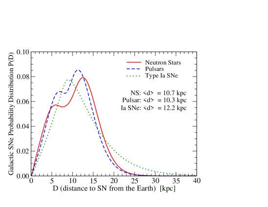
Figure 16: Probability of SN distribution in the Milky Way based on the distributions considered in Ref. Mirizzi:2006xx . The red solid, dashed blue and dotted green curves indicate, respectively, neutron star, pulsar and type Ia SN. In this work we consider the neutron star distribution (red curve) as our reference SN distribution.

In Fig. 16 we show the expected SN probability distribution in the Milky Way based on these distributions by the solid red curve. For comparison, we show the other distribution considered in Ref. Mirizzi:2006xx which are based on the pulsar (blue dashed curve) and type Ia SN (green dotted curve). We note that in calculating the shadowing probabilities rotation of the Earth was taken into account in the same way as in  Mirizzi:2006xx .

References

- (1) B. T. Cleveland, T. Daily, R. Davis, Jr., J. R. Distel, K. Lande, C. K. Lee, P. S. Wildenhain and J. Ullman, Astrophys. J. 496, 505 (1998).
- (2) K. Hirata et al. [KAMIOKANDE-II Collaboration], Phys. Rev. Lett. 58, 1490 (1987).
- (3) Y. Fukuda et al. [Super-Kamiokande Collaboration], Phys. Rev. Lett. 81, 1562 (1998) [hep-ex/9807003]; Y. Ashie et al. [Super-Kamiokande Collaboration], Phys. Rev. Lett. 93, 101801 (2004) [hep-ex/0404034].
- (4) K. Eguchi et al. [KamLAND Collaboration], Phys. Rev. Lett. 90, 021802 (2003) [hep-ex/0212021]; T. Araki et al. [KamLAND Collaboration], Phys. Rev. Lett. 94, 081801 (2005) [hep-ex/0406035].
- (5) Q. R. Ahmad et al. [SNO Collaboration], Phys. Rev. Lett. 89, 011301 (2002) [nucl-ex/0204008].
- (6) N. Smith, talk given at the 12th International conference on Topics in Astroparticle and Underground Physics (TAUP11), 5-9 September 2011, Munich, Germany, slide available at http://taup2011.mpp.mpg.de/.
- (7) http://andeslab.org/
- (8) X. Bertou, talk given at the third ANDES workshop, Valparaiso, 11 January 2012, slide available at http://andeslab.org/workshop3/presentations.php.
- (9) C. Arpesella et al. [Borexino Collaboration], Phys. Lett. B 658, 101 (2008) [arXiv:0708.2251 [astro-ph]]; Phys. Rev. Lett. 101, 091302 (2008) [arXiv:0805.3843 [astro-ph]]; G. Bellini et al. [The Borexino Collaboration], Phys. Rev. D 82, 033006 (2010) [arXiv:0808.2868 [astro-ph]]; G. Bellini, J. Benziger, D. Bick, S. Bonetti, G. Bonfini, M. Buizza Avanzini, B. Caccianiga and L. Cadonati et al., Phys. Rev. Lett. 107, 141302 (2011) [arXiv:1104.1816 [hep-ex]]; G. Bellini et al. [Borexino Collaboration], Phys. Rev. Lett. 108, 051302 (2012) [arXiv:1110.3230 [hep-ex]].
- (10) G. Bellini, J. Benziger, S. Bonetti, M. B. Avanzini, B. Caccianiga, L. Cadonati, F. Calaprice and C. Carraro et al., Phys. Lett. B 687, 299 (2010) [arXiv:1003.0284 [hep-ex]].
- (11) Y. Abe et al. [DOUBLE-CHOOZ Collaboration], Phys. Rev. Lett. 108, 131801 (2012) [arXiv:1112.6353 [hep-ex]].
- (12) F. P. An et al. [DAYA-BAY Collaboration], Phys. Rev. Lett. 108, 171803 (2012) [arXiv:1203.1669 [hep-ex]].
- (13) S. -B. K. f. R. collaboration, arXiv:1204.0626 [hep-ex].
- (14) G. Alimonti et al. [Borexino Collaboration], Astropart. Phys. 16, 205 (2002) [hep-ex/0012030].
- (15) C. Kraus et al. [SNO+ Collaboration], Prog. Part. Nucl. Phys. 64, 273 (2010).
- (16) G. Fiorentini, M. Lissia and F. Mantovani, Phys. Rept. 453, 117 (2007) [arXiv:0707.3203 [physics.geo-ph]].
- (17) S. Enomoto, Neutrino geophysics and observation of geo-neutrinos at KamLAND, PhD Thesis, http:www.awa.tohoku.ac.jp/
- (18) G. G. Raffelt, Prog. Part. Nucl. Phys. 64, 393 (2010).
- (19) R. Zukanovich Funchal, talk given at the first international workshop for the desgin of the ANDES underground laboratory, Centro Atómico Constituyentes, Buenos Aires, Argentina, 11-14 April 2011 slide avilable at http://andeslab.org/workshop1,
- (20) R. Zukanovich Funchal, talk given at the 12th International conference on Topics in Astroparticle and Underground Physics (TAUP11), 5-9 September 2011, Munich, Germany, slide avaialbe at http://taup2011.mpp.mpg.de/.
- (21) H. Nunokawa, talk given at the 11th conference on intersections of Particle and Nuclear Physics (CIPANP 2012), St. Petersburg. FL, USA, May 29-JUne 3, 2012. slide avaialbe at https://cipanp2012.triumf.ca/
- (22) T. Araki et al., Nature 436, 499 (2005).
- (23) G. Bellini et al., Phys. Lett. B 687, 299 (2010) [arXiv:1003.0284 [hep-ex]].
- (24) R. M. Bionta, G. Blewitt, C. B. Bratton, D. Casper, A. Ciocio, R. Claus, B. Cortez and M. Crouch et al., Phys. Rev. Lett. 58, 1494 (1987).
- (25) E. N. Alekseev, L. N. Alekseeva, I. V. Krivosheina and V. I. Volchenko, Phys. Lett. B 205, 209 (1988).
- (26) G. G. Raffelt, Stars as laboratories for fundamental physics: The astrophysics of neutrinos, axions, and other weakly interacting particles, Chicago, USA: Univ. Pr. (1996) 664 p
- (27) P. Antonioli, R. T. Fienberg, F. Fleurot, Y. Fukuda, W. Fulgione, A. Habig, J. Heise and A. B. McDonald et al., New J. Phys. 6, 114 (2004) [astro-ph/0406214].
- (28) http://www.iodp.org/Mission/
- (29) L. M. Krauss, S. L. Glashow and D. N. Schramm, Nature 310, 191 (1984).
- (30) R. S. Raghavan, S. .Schonert, S. Enomoto, J. Shirai, F. Suekane and A. Suzuki, Phys. Rev. Lett. 80, 635 (1998).
- (31) G. Fiorentini, F. Mantovani and B. Ricci, Phys. Lett. B 557, 139 (2003) [nucl-ex/0212008]; G. Fiorentini, M. Lissia, F. Mantovani and R. Vannucci, Phys. Rev. D 72, 033017 (2005) [hep-ph/0501111]; G. Fiorentini, M. Lissia, F. Mantovani and R. Vannucci, Earth Planet. Sci. Lett. 238, 235 (2005) [physics/0508019].
- (32) G. L. Fogli, E. Lisi, A. Palazzo and A. M. Rotunno, Earth Moon Planets 99, 111 (2006) [physics/0608025 [physics.geo-ph]]; G. L. Fogli, E. Lisi, A. Palazzo and A. M. Rotunno, Phys. Rev. D 82, 093006 (2010) [arXiv:1006.1113 [hep-ph]].
- (33) H. Nunokawa, W. J. C. Teves and R. Zukanovich Funchal, JHEP 0311, 020 (2003) [hep-ph/0308175].
- (34) A. Gando et al. [KamLAND Collaboration], Nature Geoscience 4, 647 (2011).
- (35) http://igppweb.ucsd.edu/ gabi/crust2.html
- (36) J. G. Learned, S. T. Dye and S. Pakvasa, arXiv:0810.4975 [hep-ex].
- (37) T. Lasserre, M. Fechner, G. Mention, R. Reboulleau, M. Cribier, A. Letourneau and D. Lhuillier, arXiv:1011.3850 [nucl-ex].
- (38) H. Behrens and J. Janecke, Numerical tables for beta decay and electron capture, Springer-Verlag, Berlin (1969).
- (39) G. L. Fogli, E. Lisi, A. Marrone, D. Montanino, A. Palazzo and A. M. Rotunno, arXiv:1205.5254 [hep-ph]; M. Tortola, J. W. F. Valle and D. Vanegas, arXiv:1205.4018 [hep-ph].
- (40) K. Nakamura et al. [Particle Data Group Collaboration], J. Phys. G G 37, 075021 (2010).
- (41) M. Wurm et al. [LENA Collaboration], arXiv:1104.5620 [astro-ph.IM].
- (42) G. Fiorentini, G. L. Fogli, E. Lisi, F. Mantovani and A. M. Rotunno, arXiv:1204.1923 [hep-ph].
- (43) S. V. Bergh and G. A. Tammann, Ann. Rev. Astron. Astrophys. 29, 363 (1991).
- (44) G. A. Tammann, W. Loeffler and A. Schroder, Astrophys. J. Suppl. 92, 487 (1994).
- (45) R. Diehl, H. Halloin, K. Kretschmer, G. G. Lichti, V. Schoenfelder, A. W. Strong, A. von Kienlin and W. Wang et al., Nature 439, 45 (2006) [astro-ph/0601015].
- (46) M. Ikeda et al. [Super-Kamiokande Collaboration], Astrophys. J. 669, 519 (2007) [arXiv:0706.2283 [astro-ph]].
- (47) R. Abbasi et al. [IceCube Collaboration], arXiv:1108.0171 [astro-ph.HE].
- (48) H. A. Bethe, Rev. Mod. Phys. 62, 801 (1990).
- (49) M. T. Keil, G. G. Raffelt and H. T. Janka, Astrophys. J. 590, 971 (2003) [arXiv:astro-ph/0208035].
- (50) M. T. Keil, astro-ph/0308228.
- (51) R. Buras, H.-T. Janka, M. T. Keil, G. G. Raffelt, and M. Rampp, Astrophys. J. 587, 320 (2003) [astro-ph/0205006].
- (52) A. Mirizzi, G. G. Raffelt and P. D. Serpico, JCAP 0605, 012 (2006) [arXiv:astro-ph/0604300].
- (53) A. S. Dighe and A. Y. .Smirnov, Phys. Rev. D 62, 033007 (2000) [hep-ph/9907423].
- (54) H. Duan, G. M. Fuller and Y. -Z. Qian, Phys. Rev. D 74, 123004 (2006) [astro-ph/0511275]; H. Duan, G. M. Fuller, JCarlson and Y. -Z. Qian, Phys. Rev. D 74, 105014 (2006) [astro-ph/0606616]; S. Hannestad, G. G. Raffelt, G. Sigl and Y. Y. Y. Wong, Phys. Rev. D 74, 105010 (2006) [Erratum-ibid. D 76, 029901 (2007)] [astro-ph/0608695]; G. G. Raffelt and A. Y. .Smirnov, Phys. Rev. D 76, 081301 (2007) [Erratum-ibid. D 77, 029903 (2008)] [arXiv:0705.1830 [hep-ph]]; A. Esteban-Pretel, S. Pastor, R. Tomas, G. G. Raffelt and G. Sigl, Phys. Rev. D 76, 125018 (2007) [arXiv:0706.2498 [astro-ph]]; G. L. Fogli, E. Lisi, A. Marrone and A. Mirizzi, JCAP 0712, 010 (2007) [arXiv:0707.1998 [hep-ph]]; B. Dasgupta and A. Dighe, Phys. Rev. D 77, 113002 (2008) [arXiv:0712.3798 [hep-ph]].
- (55) R. C. Schirato and G. M. Fuller, astro-ph/0205390. K. Takahashi, K. Sato, H. E. Dalhed and J. R. Wilson, Astropart. Phys. 20, 189 (2003) [astro-ph/0212195]; G. L. Fogli, E. Lisi, A. Mirizzi and D. Montanino, JCAP 0504, 002 (2005) [hep-ph/0412046].
- (56) G. L. Fogli, E. Lisi, A. Mirizzi and D. Montanino, JCAP 0606, 012 (2006) [hep-ph/0603033].
- (57) A. Friedland and A. Gruzinov, astro-ph/0607244.
- (58) T. Fischer, S. C. Whitehouse, A. Mezzacappa, F. -K. Thielemann and M. Liebendorfer, Astron. Astrophys. 517, A80 (2010) [arXiv:0908.1871 [astro-ph.HE]].
- (59) L. Hudepohl, B. Muller, H. -T. Janka, A. Marek and G. G. Raffelt, Phys. Rev. Lett. 104, 251101 (2010) [Erratum-ibid. 105, 249901 (2010)] [arXiv:0912.0260 [astro-ph.SR]].
- (60) T. Fischer, G. Martinez-Pinedo, M. Hempel and M. Liebendorfer, Phys. Rev. D 85, 083003 (2012) [arXiv:1112.3842 [astro-ph.HE]].
- (61) C. Lunardini, B. Muller and H. -T. .Janka, Phys. Rev. D 78, 023016 (2008) [arXiv:0712.3000 [astro-ph]].
- (62) S. Chakraborty, T. Fischer, A. Mirizzi, N. Saviano and R. Tomas, Phys. Rev. Lett. 107, 151101 (2011) [arXiv:1104.4031 [hep-ph]].
- (63) S. Sarikas, G. G. Raffelt, L. Hudepohl and H. -T. Janka, Phys. Rev. Lett. 108, 061101 (2012) [arXiv:1109.3601 [astro-ph.SR]].
- (64) C. Lunardini, Phys. Rev. Lett. 102, 231101 (2009) [arXiv:0901.0568 [astro-ph.SR]].
- (65) K. Abe et al. [T2K Collaboration], Phys. Rev. Lett. 107, 041801 (2011) [arXiv:1106.2822 [hep-ex]].
- (66) P. Adamson et al. [MINOS Collaboration], Phys. Rev. Lett. 107, 181802 (2011) [arXiv:1108.0015 [hep-ex]].
- (67) P. A. N. Machado, H. Minakata, H. Nunokawa and R. Zukanovich Funchal, arXiv:1111.3330 [hep-ph].
- (68) J. F. Beacom, W. M. Farr and P. Vogel, Phys. Rev. D 66, 033001 (2002) [hep-ph/0205220].
- (69) B. Dasgupta and J. .F. Beacom, Phys. Rev. D 83, 113006 (2011) [arXiv:1103.2768 [hep-ph]].
- (70) H. Minakata, H. Nunokawa, R. Tomas and J. W. F. Valle, Phys. Lett. B 542, 239 (2002) [hep-ph/0112160].
- (71) S. Skadhauge and R. Zukanovich Funchal, JCAP 0704, 014 (2007) [hep-ph/0611194].
- (72) K. Abe, T. Abe, H. Aihara, Y. Fukuda, Y. Hayato, K. Huang, A. K. Ichikawa and M. Ikeda et al., arXiv:1109.3262 [hep-ex].
- (73) H. Minakata, H. Nunokawa, R. Tomas and J. W. F. Valle, JCAP 0812, 006 (2008) [arXiv:0802.1489 [hep-ph]].
- (74) L. Cadonati, F. P. Calaprice and M. C. Chen, Astropart. Phys. 16, 361 (2002) [hep-ph/0012082].
- (75) C. Lunardini, A. Yu. .Smirnov, Nucl. Phys. B616, 307-348 (2001). [hep-ph/0106149].
- (76) A. S. Dighe, M. T. Keil and G. G. Raffelt, JCAP 0306, 006 (2003) [arXiv:hep-ph/0304150].
- (77) A. S. Dighe, M. Kachelriess, G. G. Raffelt, R. Tomas, JCAP 0401, 004 (2004). [hep-ph/0311172].
- (78) G. Bari et al. [LVD Collaboration], Nucl. Instrum. Meth. A 277, 11 (1989).
- (79) A. M. Dziewonski and D. L. Anderson, Phys. Earth Planet. Interiors 25, 297 (1981).
- (80) E. K. Akhmedov, M. Maltoni and A. Y. .Smirnov, JHEP 0705, 077 (2007) [hep-ph/0612285]; E. K. .Akhmedov, M. Maltoni and A. Y. .Smirnov, JHEP 0806, 072 (2008) [arXiv:0804.1466 [hep-ph]].
- (81) S. Abe et al. [KamLAND Collaboration], Phys. Rev. C 84, 035804 (2011) [arXiv:1106.0861 [hep-ex]].
- (82) J. Kumar, J. G. Learned, M. Sakai and S. Smith, Phys. Rev. D 84, 036007 (2011) [arXiv:1103.3270 [hep-ph]].
- (83) A. Strumia and F. Vissani, Phys. Lett. B 564, 42 (2003) [astro-ph/0302055].
- (84) S. Weinberg, Phys. Rev. D 5, 1412 (1972).
- (85) I. Yusifov and I. Küçük, Astron. Astrophys. 422, 545 (2004) [astro-ph/0405559].
- (86) http://www.nist.gov/
- (87) A. Gando et al. [The KamLAND Collaboration], Phys. Rev. D 83, 052002 (2011) [arXiv:1009.4771 [hep-ex]].