Nonlinear spectral unmixing of hyperspectral images using Gaussian processes

Abstract

This paper presents an unsupervised algorithm for nonlinear unmixing of hyperspectral images. The proposed model assumes that the pixel reflectances result from a nonlinear function of the abundance vectors associated with the pure spectral components. We assume that the spectral signatures of the pure components and the nonlinear function are unknown. The first step of the proposed method consists of the Bayesian estimation of the abundance vectors for all the image pixels and the nonlinear function relating the abundance vectors to the observations. The endmembers are subsequently estimated using Gaussian process regression. The performance of the unmixing strategy is evaluated with simulations conducted on synthetic and real data.

I Introduction

Spectral unmixing (SU) is a major issue when analyzing hyperspectral images. It consists of identifying the macroscopic materials present in an hyperspectral image and quantifying the proportions of these materials in the image pixels. Many SU strategies assume that pixel reflectances are linear combinations of pure component spectra [1]. The resulting linear mixing model (LMM) has been widely adopted in the literature and has provided some interesting results. However, as discussed in [1], the LMM can be inappropriate for some hyperspectral images, such as those containing sand, trees or vegetation areas. Nonlinear mixing models provide an interesting alternative to overcome the inherent limitations of the LMM. Nonlinear mixing models recently proposed in the literature include the bidirectional reflectance-based model of [2] for hyperspectral images including intimate mixtures, i.e., when the photons are intereacting with all the materials simultaneously. Such mixtures may occur for instance in sand or mineral areas. Another class of nonlinear model referred to as bilinear models have been studied in [3, 4, 5, 6] for modeling scattering effects (mainly observed in vegetation areas). Other more flexible unmixing techniques have been also proposed to handle wider classes of nonlinearity, including radial basis function networks [7, 8] post-nonlinear mixing models [9] and kernel-based models [10, 11, 12, 13].

Most existing unmixing strategies can be decomposed into two steps referred to as endmember extraction and abundance estimation. Endmember identification is usually achieved before estimating the abundances for all the image pixels. In the last decade, many endmember extraction algorithms (EEAs) have been developed to identify the pure spectral components contained in a hyperspectral image (see [1] for a recent review of these methods). Most EEAs rely on the LMM, which, as discussed, is inappropriate for the case of nonlinear mixtures of the endmembers. More recently, an EEA was proposed in [14] to extract endmembers from a set of nonlinearly mixed pixels. This paper proposes first to estimate the abundance vectors and to estimate the endmembers during a second step, using the prediction capacity of Gaussian processes (GPs). This approach breaks from the usual paradigm of spectral unmixing. More precisely, this paper considers a kernel-based approach for nonlinear SU based on a nonlinear dimensionality reduction using a Gaussian process latent variable model (GPLVM). The main advantage of GPLVMs is their capacity to accurately model many different nonlinearities. In this paper, we propose to use a particular form of kernel based on existing bilinear models, which allows the proposed unmixing strategy to be accurate when the underlying mixing model is bilinear. Note that the LMM is a particular bilinear model. The algorithm proposed herein is “unsupervised” in the sense that the endmembers contained in the image and the mixing model are not known. Only the number of endmembers is assumed to be known. As a consequence, the parameters to be estimated are the kernel parameters, the endmember spectra and the abundances for all image pixels.

The paper is organized as follows. Section II presents the nonlinear mixing model considered in this paper for hyperspectral image unmixing. Section III introduces the GPLVM used for latent variable estimation. The constrained GPLVM for abundance estimation is detailed in Section IV. Section V studies the endmember estimation procedure using GP regression. Some simulation results conducted on synthetic data are shown and discussed in Section VI. Finally, conclusions are drawn in Section VII.

II Nonlinear mixing model

Consider a hyperspectral image of $N$ pixels, composed of $R$ endmembers and observed in $L$ spectral bands. For convenience, the data are assumed to have been previously centered. The $L$-spectrum $\mathbf{y}(n)=[y_{1}(n),\ldots,y_{L}(n)]^{T}$ of the $n$th mixed pixel ($n=1,\ldots,N$) is defined as a transformation of its corresponding abundance vector ${\boldsymbol{a}}(n)=[a_{1}(n),\ldots,a_{R}(n)]^{T}$ as follows

$$\mathbf{y}(n) = \boldsymbol{g}\left[{\boldsymbol{a}}(n)\right]+{\mathbf{e}}(n),\quad n=1,\ldots,N$$ (1)

where $\boldsymbol{g}:\mathbb{R}^{R}\rightarrow\mathbb{R}^{L}$ is a linear or nonlinear unknown function. The noise vector ${\mathbf{e}}(n)$ is an independent, identically distributed (i.i.d.) white Gaussian noise sequence with variance $\sigma^{2}$, i.e., ${\mathbf{e}}(n)\sim\mathcal{N}\left({\mathbf{e}}(n)|\boldsymbol{0}_{L},\sigma^{2}\textbf{I}_{L}\right),n=1,\ldots,N$. Without loss generality, the nonlinear mapping (1) from the abundance space to the observation space can be rewritten

$$\mathbf{y}(n) = \boldsymbol{W}_{0}{\boldsymbol{\psi}}\left[{\boldsymbol{a}}(n)\right]+{\mathbf{e}}(n),\quad n=1,\ldots,N$$ (2)

where ${\boldsymbol{\psi}}:\mathbb{R}^{R}\rightarrow\mathbb{R}^{D}$, $\boldsymbol{W}_{0}$ is an $L\times D$ matrix and the dimension $D$ is the dimension of the subspace spanned by the transformed abundance vectors ${\boldsymbol{\psi}}\left[{\boldsymbol{a}}(n)\right],n=1,\ldots,N$. Of course, the performance of the unmixing strategy relies on the choice of the nonlinear function ${\boldsymbol{\psi}}$. In this paper, we will use the following nonlinearity

$${\boldsymbol{\psi}}: \mathbb{R}^{R} \rightarrow\mathbb{R}^{D}$$ (3)

$${\boldsymbol{a}} \mapsto{\boldsymbol{\psi}}\left[{\boldsymbol{a}}\right]=\left[a_{1},\ldots,a_{R},a_{1}a_{2}\ldots,a_{R-1}a_{R}\right]^{T},$$

with $D=R(R+1)/2$. The primary motivation for considering this particular kind of nonlinearity is the fact that the resulting mixing model is a bilinear model with respect to each abundance $a_{r},r=1,\ldots,R$. More precisely, this mixing model extends the generalized bilinear model proposed in [6] and thus the LMM. It is important to note from (2) and (3) that $\boldsymbol{W}_{0}$ contains the $R$ spectra of the pure components present in the image and $R(R-1)/2$ interaction spectra between these components. Note also that the analysis presented in this paper could be applied to any other nonlinearity ${\boldsymbol{\psi}}$.

Due to physical constraints, the abundance vector ${\boldsymbol{a}}(n)=[a_{1}(n),\ldots,a_{R}(n)]^{T}$ satisfies the following positivity and sum-to-one constraints

$$\sum_{r=1}^{R}{a_{r}(n)}=1,~{}~{}a_{r}(n)\geq 0,\forall r\in\left\{1,\ldots,R\right\}.$$ (4)

Since the nonlinearity ${\boldsymbol{\psi}}$ is fixed, the problem of unsupervised spectral unmixing is to determine the $L\times D$ spectrum matrix $\boldsymbol{W}_{0}$, the $N\times R$ abundance matrix ${\mathbb{A}}=[{\boldsymbol{a}}(1),\ldots,{\boldsymbol{a}}(N)]^{T}$ satisfying (2) under the constraints (4) and the noise variance $\sigma^{2}$. Unfortunately, it can be shown that the solution of this constrained problem is not unique. In the noise-free linear case, it is well known that the data are contained in a simplex whose vertices are the endmembers. When estimating the endmembers in the linear case, a simplex of minimum volume embedding the data is expected. Equivalently, the estimated abundance vectors are expected to occupy the largest volume in the simplex defined by (4). In a similar fashion to the linear case, the estimated abundance matrix resulting from an unsupervised nonlinear SU strategy may not occupy the largest volume in the simplex defined by (4). To tackle this problem, we first propose to relax the positivity constraints for the elements of the matrix ${\mathbb{A}}$ and to consider only the sum-to-one constraint. For ease of understanding, we introduce $R\times 1$ vectors satisfying the sum-to-one constraint

$$\sum_{r=1}^{R}{x_{r}(n)}=1,\quad n=1,\ldots,N$$ (5)

referred to as latent variables and denoted as $\boldsymbol{x}(n)=[x_{1}(n),\ldots,x_{R}(n)]^{T},n=1,\ldots,N$. The positivity constraint will be handled subsequently by a scaling procedure discussed in Section IV. The next section presents the Bayesian model for latent variable estimation using GPLVMs.

III Bayesian model

GPLVMs [15] are powerful tools for probabilistic nonlinear dimensionality reduction that rewrite the nonlinear model (1) as a nonlinear mapping from a latent space to the observation space as follows

$$\mathbf{y}(n) = \boldsymbol{W}{\boldsymbol{\psi}}\left[\boldsymbol{x}(n)\right]+{\mathbf{e}}(n),\quad n=1,\ldots,N$$ (6)

where ${\boldsymbol{\psi}}$ is defined in (3), $\boldsymbol{W}=[\boldsymbol{w}_{1},\ldots,\boldsymbol{w}_{L}]^{T}$ is an $L\times D$ matrix with $\boldsymbol{w}_{\ell}=[w_{\ell,1},\ldots,w_{\ell,D}]^{T}$, and $D=R(R+1)/2$. Note that from (2) and (6) the columns of $\boldsymbol{W}$ span the same subspace as the columns of $\boldsymbol{W}_{0}$. Consequently, the columns of $\boldsymbol{W}$ are linear combinations of the spectra of interest, i.e., the columns of $\boldsymbol{W}_{0}$. Note also that when $\boldsymbol{W}$ is full rank, it can be shown that the latent variables are necessarily linear combinations of the abundance vectors of interest. Figs. 1 and 2 illustrate the mapping from the abundance vectors to the observations that will be used in this paper. Note that the linear mapping between the abundances and the latent variables will be explained in detail in Section IV. For brevity, the $D\times 1$ vectors ${\boldsymbol{\psi}}\left[\boldsymbol{x}(n)\right]$ will be denoted as ${\boldsymbol{\psi}}_{x}(n)$ in the sequel. Assuming independence between the observations, the statistical properties of the noise lead to the following likelihood of the $N\times L$ observation matrix $\mathbf{Y}=[\mathbf{y}(1),\ldots,\mathbf{y}(N)]^{T}$

$$\mathbf{Y}|\boldsymbol{W},{\boldsymbol{X}},\sigma^{2}\sim\prod_{n=1}^{N}\mathcal{N}\left(\mathbf{y}(n)|\boldsymbol{W}{\boldsymbol{\psi}}_{x}(n),\sigma^{2}\textbf{I}_{L}\right)$$ (7)

where ${\boldsymbol{X}}=[\boldsymbol{x}(1),\ldots,\boldsymbol{x}(N)]^{T}$ is the $N\times R$ latent variable matrix. Note that the likelihood can be rewritten as a product of Gaussian distributions over the spectral bands as follows

$$\mathbf{Y}|\boldsymbol{W},{\boldsymbol{X}},\sigma^{2}\sim\prod_{\ell=1}^{L}\mathcal{N}\left(\mathbf{y}_{\ell}|{\boldsymbol{\Psi}}_{x}\boldsymbol{w}_{\ell},\sigma^{2}\textbf{I}_{L}\right)$$ (8)

where $\mathbf{Y}=[\mathbf{y}_{1},\ldots,\mathbf{y}_{L}]$ and ${\boldsymbol{\Psi}}_{x}=[{\boldsymbol{\psi}}_{x}(1),\ldots,{\boldsymbol{\psi}}_{x}(N)]^{T}$ is an $N\times D$ matrix. The idea of GPLVMs is to consider $\boldsymbol{W}$ as a nuisance parameter, to assign a Gaussian prior to $\boldsymbol{W}$ and to marginalize the joint likelihood (7) over $\boldsymbol{W}$, i.e.,

$$f(\mathbf{Y}|{\boldsymbol{X}},\sigma^{2})=\int f(\mathbf{Y}|\boldsymbol{W},{\boldsymbol{X}},\sigma^{2})f(\boldsymbol{W})\mathrm{d}\boldsymbol{W}$$ (9)

where $f(\boldsymbol{W})$ is the prior distribution of $\boldsymbol{W}$. The estimation of ${\boldsymbol{X}}$ and $\sigma^{2}$ can then be achieved by maximizing (9) following the maximum likelihood estimator (MLE) principle. An alternative consists of using an appropriate prior distribution $f({\boldsymbol{X}},\sigma^{2})$, assuming prior independence between $\boldsymbol{W}$ and $({\boldsymbol{X}},\sigma^{2})$, and maximizing the joint posterior distribution

$$f({\boldsymbol{X}},\sigma^{2}|\mathbf{Y}) \propto \int f(\mathbf{Y}|\boldsymbol{W},{\boldsymbol{X}},\sigma^{2})f(\boldsymbol{W})f({\boldsymbol{X}},\sigma^{2})\mathrm{d}\boldsymbol{W}$$ (10)

$$\propto f({\boldsymbol{X}},\sigma^{2})\int f(\mathbf{Y}|\boldsymbol{W},{\boldsymbol{X}},\sigma^{2})f(\boldsymbol{W})\mathrm{d}\boldsymbol{W}$$

$$\propto f(\mathbf{Y}|{\boldsymbol{X}},\sigma^{2})f({\boldsymbol{X}},\sigma^{2})$$

with respect to (w.r.t.) $({\boldsymbol{X}},\sigma^{2})$, yielding the maximum a posteriori (MAP) estimator of $({\boldsymbol{X}},\sigma^{2})$. The next paragraph discusses different possibilities for marginalizing the joint likelihood (8) w.r.t. $\boldsymbol{W}$.

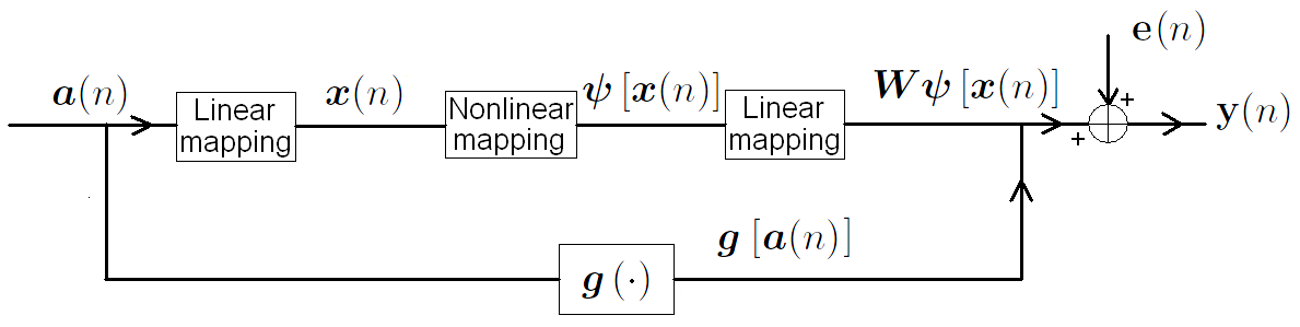
Figure 1: Nonlinear mapping from the abundances vectors to the observed mixed pixels.

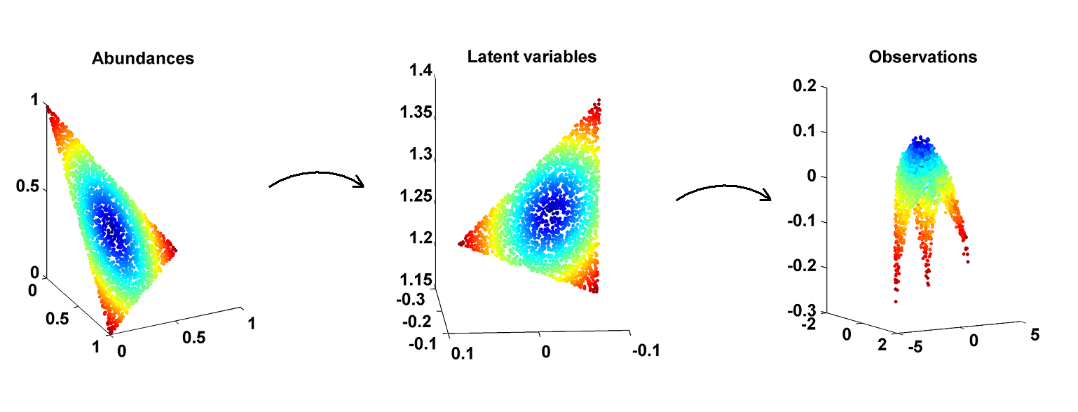
Figure 2: Example of mapping decomposition from the abundance vectors to the observed nonlinearly mixed pixels through the latent variables ($R=3$).

III-A Marginalizing $\boldsymbol{W}$

It can be seen from (9) that the marginalized likelihood and thus the associated latent variables depend on the choice of the prior $f(\boldsymbol{W})$. More precisely, assigning a given prior for $\boldsymbol{W}$ favors particular representations of the data, i.e., particular solutions for the latent variable matrix ${\boldsymbol{X}}$ maximizing the posterior (10). When using GPLVMs for dimensionality reduction, a classical choice [15] consists of assigning independent Gaussian priors for $\boldsymbol{w}_{1},\ldots,\boldsymbol{w}_{L}$, leading to

$$f(\boldsymbol{W})=\left(\dfrac{1}{2\pi}\right)^{\frac{DL}{2}}\prod_{\ell=1}^{L}\exp\left[-\dfrac{1}{2}\left\|\boldsymbol{w}_{\ell}\right\|^{2}\right].$$ (11)

However, this choice can be inappropriate for SU. First, Eq. (11) can be incompatible with the admissible latent space, constrained by (5). Second, the prior (11) assumes the columns of $\boldsymbol{W}$ (linear combinations of the spectra of interest) are a priori Gaussian, which is not relevant for real spectra in most applications. A more sophisticated choice consists of considering a priori correlation between the columns (inter-spectra correlation) and rows (inter-bands correlation) of $\boldsymbol{W}$ using a structured covariance matrix to be fixed or estimated. In particular, introducing correlation between close spectral bands is of particular interest in hyperspectral imagery. Structured covariance matrices have already been considered in the GP literature for vector-valued kernels [16] (see [17] for a recent review). However, computing the resulting marginalized likelihood usually requires the estimation of the structured covariance matrix and the inversion of an $NL\times NL$ covariance matrix, which is prohibitive for SU of hyperspectral images since several hundreds of spectral bands are usually considered when analyzing real data. Sparse approximation techniques might be used to reduce this computational complexity (see [19] for a recent review). However, to our knowledge, these techniques rely on the inversion of matrices bigger than $N\times N$ matrices. The next section presents an alternative that only requires the inversion of an $D\times D$ covariance matrix without any approximation.

III-B Subspace identification

It can be seen from (6) that in the noise-free case, the data belong to a $D$-dimensional subspace that is spanned by the columns of $\boldsymbol{W}$. To reduce the computational complexity induced by the marginalization of the matrix $\boldsymbol{W}$ while considering correlations between spectral bands, we propose to marginalize a basis of the subspace spanned by $\boldsymbol{W}$ instead of $\boldsymbol{W}$ itself. More precisely, $\boldsymbol{W}$ can be decomposed as follows

$$\boldsymbol{W}=\boldsymbol{P}\boldsymbol{U}^{T}$$ (12)

where $\boldsymbol{P}=[\boldsymbol{p}_{1},\ldots,\boldsymbol{p}_{L}]^{T}$ is an $L\times D$ matrix ($\boldsymbol{p}_{\ell}$ is $D\times 1$ vector) whose columns are arbitrary basis vectors of the $D$-dimensional subspace that contains the subspace spanned by the columns of $\boldsymbol{W}$ and $\boldsymbol{U}=[\boldsymbol{u}_{1},\ldots,\boldsymbol{u}_{D}]^{T}$ is a $D\times D$ matrix that scales the columns of $\boldsymbol{P}$. Note that the subspaces spanned by $\boldsymbol{P}$ and $\boldsymbol{W}$ are the same when $\boldsymbol{W}$ is full rank, resulting in a full rank matrix $\boldsymbol{U}$. The joint likelihood (8) can be rewritten as

$$\mathbf{Y}|\boldsymbol{P},\boldsymbol{U},{\boldsymbol{X}},\sigma^{2}\sim\prod_{\ell=1}^{L}\mathcal{N}\left(\mathbf{y}_{\ell}|\boldsymbol{C}\boldsymbol{p}_{\ell},\sigma^{2}\textbf{I}_{L}\right)$$ (13)

where $\boldsymbol{C}={\boldsymbol{\Psi}}_{x}\boldsymbol{U}$ is an $N\times D$ matrix. The proposed subspace estimation procedure consists of assigning an appropriate prior distribution to $\boldsymbol{P}$ (denoted as $f(\boldsymbol{P})$) and to marginalize $\boldsymbol{P}$ from the joint posterior of interest. It is easier to choose an informative prior distribution $f(\boldsymbol{P})$ that accounts for correlation between spectral bands than choosing an informative $f(\boldsymbol{W})$ since $\boldsymbol{P}$ is an arbitrary basis of the subspace spanned by $\boldsymbol{W}$, which can be easily estimated (as will be shown in the next section).

III-C Parameter priors

GPLVMs construct a smooth mapping from the latent space to the observation space that preserves dissimilarities [20]. In the SU context, it means that pixels that are spectrally different have different latent variables and thus different abundance vectors. However, preserving local distances is also interesting: spectrally close pixels are expected to have similar abundance vectors and thus similar latent variables. Several approaches have been proposed to preserve similarities, including back-constraints [20], dynamical models [21] and locally linear embedding (LLE) [22]. In this paper, we use LLE to assign an appropriate prior to ${\boldsymbol{X}}$. First, the $K$ nearest neighbors $\{\mathbf{y}(j)\}_{j\in\mathcal{\nu}_{i}}$ of each observation vector $\mathbf{y}(i)$ are computed using the Euclidian distance ($\mathcal{\nu}_{i}$ is the set of integers $j$ such that $\mathbf{y}(j)$ is a neighbor of $\mathbf{y}(i)$). The weight matrix $\boldsymbol{\Lambda}_{\mathrm{LLE}}=[\lambda_{i,j}]$ of size $N\times N$ providing the best reconstruction of $\mathbf{y}(i)$ from its neighbors is then estimated as

$$\boldsymbol{\Lambda}_{\mathrm{LLE}}=\arg\underset{\boldsymbol{\Lambda}}{\min}\sum_{i=1}^{N}\left\|\mathbf{y}(i)-\sum_{j\in\mathcal{\nu}_{i}}{\lambda_{i,j}\mathbf{y}(j)}\right\|^{2}.$$ (14)

Note that the solution of (14) is easy to obtain in closed form since the criterion to optimize is a quadratic function of $\boldsymbol{\Lambda}$. Note also that the matrix $\boldsymbol{\Lambda}$ is sparse since each pixel is only described by its $K$ nearest neighbors. The locally linear patches obtained by the LLE can then be used to set the following prior for the latent variable matrix

$$f({\boldsymbol{X}}|\boldsymbol{\Lambda}_{\mathrm{LLE}},\gamma) \propto \exp\left[-\dfrac{\gamma}{2}\sum_{i=1}^{N}\left\|\boldsymbol{x}(i)-\sum_{j\in\mathcal{\nu}_{i}}{\lambda_{i,j}\boldsymbol{x}(j)}\right\|^{2}\right]$$ (15)

$$\times \prod_{n=1}^{N}{\boldsymbol{1}}_{\mathcal{D}}\left[\boldsymbol{x}(n)\right]$$

where $\gamma$ is a fixed hyperparameter to be adjusted and ${\boldsymbol{1}}_{\mathcal{D}}(\cdot)$ is the indicator function over the set $\mathcal{D}$ defined by the constraints (5).

In this paper, we propose to assign a prior to $\boldsymbol{P}$ using the standard principal component analysis (PCA) (note again that the data have been centered). Assuming prior independence between $\boldsymbol{p}_{1},\ldots,\boldsymbol{p}_{L}$, the following prior is considered for the matrix $\boldsymbol{P}$

$$f\left(\boldsymbol{P}|\overline{\boldsymbol{P}},s^{2}\right)=\left(\dfrac{1}{2\pi s^{2}}\right)^{\frac{NL}{2}}\prod_{\ell=1}^{L}\exp\left[-\dfrac{1}{2s^{2}}\left\|\boldsymbol{p}_{\ell}-\bar{\boldsymbol{p}}_{\ell}\right\|^{2}\right]$$ (16)

where $\overline{\boldsymbol{P}}=[\bar{\boldsymbol{p}}_{1},\ldots,\bar{\boldsymbol{p}}_{L}]^{T}$ is an $L\times D$ projection matrix containing the first $D$ eigenvectors of the sample covariance matrix of the observations (provided by PCA) and $s^{2}$ is a dispersion parameter that controls the dispersion of the prior. Note that the correlation between spectral bands is implicitly introduced through $\overline{\boldsymbol{P}}$.

Non-informative priors are assigned to the noise variance $\sigma^{2}$ and the matrix $\boldsymbol{U}$, i.e,

$$\begin{array}[]{ccc}f(\sigma^{2})&\propto&{\boldsymbol{1}}_{(0,\delta_{\sigma^{2}})}(\sigma^{2})\\ f(u_{i,j})&\propto&{\boldsymbol{1}}_{(-\delta_{\boldsymbol{U}},\delta_{\boldsymbol{U}})}(u_{i,j})\\ \end{array}$$ (19)

where the intervals $(0,\delta_{\sigma^{2}})$ and $(-\delta_{\boldsymbol{U}},\delta_{\boldsymbol{U}})$ cover the possible values of the parameters $\sigma^{2}$ and $\boldsymbol{U}$. Similarly, the following non-informative prior is assigned to the hyperparameter $s^{2}$

$$f(s^{2}) \propto {\boldsymbol{1}}_{(0,\delta_{s^{2}})}(s^{2})$$ (20)

where the interval $(0,\delta_{s^{2}})$ covers the possible values of the hyperparameter $s^{2}$. The resulting directed acyclic graph (DAG) is depicted in Fig. 3.

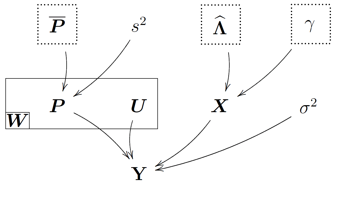
Figure 3: DAG for the parameter priors and hyperpriors (the fixed parameters appear in dashed boxes).

III-D Marginalized posterior distribution

Assuming prior independence between $\boldsymbol{P}$, ${\boldsymbol{X}}$, $\boldsymbol{U}$, $s^{2}$ and $\sigma^{2}$, the marginalized posterior distribution of $\boldsymbol{\theta}=({\boldsymbol{X}},\boldsymbol{U},s^{2},\sigma^{2})$ can be expressed as

$f\left(\boldsymbol{\theta}|\mathbf{Y},{\boldsymbol{\Lambda}}_{\mathrm{LLE}},\overline{\boldsymbol{P}},\gamma\right)$

$$\propto f(\boldsymbol{\theta}|{\boldsymbol{\Lambda}}_{\mathrm{LLE}},\gamma)\int f(\mathbf{Y}|\boldsymbol{P},\boldsymbol{\theta})f\left(\boldsymbol{P}|\overline{\boldsymbol{P}},s^{2}\right)\mathrm{d}\boldsymbol{P}$$ (21)

$$\propto f(\mathbf{Y}|\boldsymbol{\theta},\overline{\boldsymbol{P}})f(\boldsymbol{\theta}|{\boldsymbol{\Lambda}}_{\mathrm{LLE}},\gamma)$$

where $f(\boldsymbol{\theta}|{\boldsymbol{\Lambda}}_{\mathrm{LLE}},\gamma)=f({\boldsymbol{X}}|{\boldsymbol{\Lambda}}_{\mathrm{LLE}},\gamma)f(\boldsymbol{U})f(s^{2})f(\sigma^{2})$. Straightforward computations leads to

$$f(\mathbf{Y}|\boldsymbol{\theta},\overline{\boldsymbol{P}}) = \int f(\mathbf{Y}|\boldsymbol{P},\boldsymbol{\theta})f\left(\boldsymbol{P}|\overline{\boldsymbol{P}},s^{2}\right)\mathrm{d}\boldsymbol{P}$$ (22)

$$\propto \prod_{\ell=1}^{L}\dfrac{1}{|{\boldsymbol{\Sigma}}|^{\frac{1}{2}}}\exp\left[-\dfrac{1}{2}\bar{\mathbf{y}}_{\ell}^{T}{\boldsymbol{\Sigma}}^{-1}\bar{\mathbf{y}}_{\ell}\right]$$

$$\propto |{\boldsymbol{\Sigma}}|^{-\frac{L}{2}}\exp\left[-\dfrac{1}{2}\textrm{tr}({\boldsymbol{\Sigma}}^{-1}\bar{\mathbf{Y}}\bar{\mathbf{Y}}^{T})\right]$$

where ${\boldsymbol{\Sigma}}=s^{2}\boldsymbol{C}\boldsymbol{C}^{T}+\sigma^{2}\textbf{I}_{N}$, $\bar{\mathbf{y}}_{\ell}=\mathbf{y}_{\ell}-\boldsymbol{C}\bar{\boldsymbol{p}}_{\ell}$ is an $N\times 1$ vector, $\bar{\mathbf{Y}}=[\bar{\mathbf{y}}_{1},\ldots,\bar{\mathbf{y}}_{L}]=\mathbf{Y}-\boldsymbol{C}\overline{\boldsymbol{P}}^{T}$ is an $N\times L$ matrix and $\textrm{tr}(\cdot)$ denotes the matrix trace.

Mainly due to the nonlinearity introduced through the nonlinear mapping, a closed form expression for the parameters maximizing the joint posterior distribution (21) is impossible to obtain. We propose to use a scaled conjugate gradient (SCG) method to maximize the marginalized log-posterior. To ensure the sum-to-one constraint for ${\boldsymbol{X}}$, the following arbitrary reparametrization

$$x_{R}(n)=1-\sum_{r=1}^{R-1}{x_{r}(n)},\quad n=1,\ldots,N$$

is used and the marginalized posterior distribution is optimized w.r.t. the first $(R-1)$ columns of ${\boldsymbol{X}}$ denoted ${\boldsymbol{X}}_{\backslash R}$. The partial derivatives of the log-posterior w.r.t. ${\boldsymbol{X}}_{\backslash R},\boldsymbol{U},s^{2}$ and $\sigma^{2}$ are obtained using partial derivatives w.r.t. ${\boldsymbol{\Sigma}}$ and $\bar{\mathbf{Y}}$ and the classical chain rules (see technical report [18] for further details). The resulting latent variable estimation procedure is referred to as locally linear GPLVM (LL-GPLVM).

Note that the marginalized likelihood reduces to the product of $L$ independent Gaussian probability density functions since

$$\mathbf{y}_{\ell}|\bar{\boldsymbol{p}}_{\ell},\boldsymbol{U},{\boldsymbol{X}},\sigma^{2},s^{2}\sim\mathcal{N}\left(\boldsymbol{C}\bar{\boldsymbol{p}}_{\ell},s^{2}\boldsymbol{C}\boldsymbol{C}^{T}+\sigma^{2}\textbf{I}_{N}\right)$$ (23)

and $\ell=1,\ldots,L$. Note also that the covariance matrix ${\boldsymbol{\Sigma}}=s^{2}\boldsymbol{C}\boldsymbol{C}^{T}+\sigma^{2}\textbf{I}_{N}$ is related to the covariance matrix of the $2$nd order polynomial kernel [23, p. 89]. More precisely, the proposed nonlinear mapping corresponds to a particular polynomial kernel whose metric is induced by the matrix $\boldsymbol{U}$. Finally, note that the evaluation of the marginalized likelihood (22) only requires the inversion of the $N\times N$ covariance matrix ${\boldsymbol{\Sigma}}$. It can been seen from the following Woodbury matrix identity [24]

$${\boldsymbol{\Sigma}}^{-1}=\sigma^{-2}\left[\textbf{I}_{N}-\boldsymbol{C}\left(\sigma^{2}s^{-2}\textbf{I}_{D}+\boldsymbol{C}^{T}\boldsymbol{C}\right)^{-1}\boldsymbol{C}^{T}\right]$$ (24)

that the computation of ${\boldsymbol{\Sigma}}^{-1}$ mainly relies on the inversion of a $D\times D$ matrix. Similarly, the computation of $|{\boldsymbol{\Sigma}}|=1/|{\boldsymbol{\Sigma}}^{-1}|$ mainly consists of computing the determinant of a $D\times D$ matrix, which reduces the computational cost when compared to the structured covariance matrix based approach presented in Section III-A.

III-E Estimation of $\boldsymbol{P}$

Let us denote as $\hat{\boldsymbol{\theta}}=(\widehat{{\boldsymbol{X}}},\widehat{\boldsymbol{U}},\hat{s}^{2},\hat{\sigma}^{2})$ the maximum a posteriori (MAP) estimator of $\boldsymbol{\theta}=({\boldsymbol{X}},\boldsymbol{U},s^{2},\sigma^{2})$ obtained by maximizing $\eqref{eq:posterior_X}$. Using the likelihood (13), the prior distribution (16) and Bayes’ rule, we obtain the posterior distribution of $\boldsymbol{P}$ conditioned upon $\boldsymbol{\theta}$, i.e.,

$$\boldsymbol{P}|\mathbf{Y},\boldsymbol{\theta},\overline{\boldsymbol{P}}\sim\prod_{\ell=1}^{L}\mathcal{N}\left(\boldsymbol{p}_{\ell}|\hat{\boldsymbol{p}}_{\ell}\,{\boldsymbol{S}}\right)$$ (25)

where ${\boldsymbol{S}}^{-1}=\sigma^{-2}\boldsymbol{C}^{T}\boldsymbol{C}+s^{-2}\textbf{I}_{D}$ and $\hat{\boldsymbol{p}}_{\ell}={\boldsymbol{S}}(\boldsymbol{C}^{T}\mathbf{y}_{\ell}-\bar{\boldsymbol{p}}_{\ell})$. Since the conditional posterior distribution of $\boldsymbol{P}$ is the product of $L$ independent Gaussian distributions, the MAP estimator of $\boldsymbol{P}$ conditioned upon $\hat{\boldsymbol{\theta}}$ is given by

$$\widehat{\boldsymbol{P}}=\left(\mathbf{Y}^{T}\widehat{\boldsymbol{C}}-\overline{\boldsymbol{P}}\right)\widehat{{\boldsymbol{S}}}$$ (26)

where $\widehat{{\boldsymbol{S}}}^{-1}=\hat{\sigma}^{-2}\widehat{\boldsymbol{C}}^{T}\widehat{\boldsymbol{C}}+\hat{s}^{-2}\textbf{I}_{D}$, $\widehat{\boldsymbol{C}}=\widehat{{\boldsymbol{\Psi}}}_{x}\widehat{\boldsymbol{U}}$, $\widehat{{\boldsymbol{\Psi}}}_{x}=[{\boldsymbol{\psi}}_{\hat{x}}(1),\ldots,{\boldsymbol{\psi}}_{\hat{x}}(N)]^{T}$ and $\widehat{{\boldsymbol{X}}}=[\hat{\boldsymbol{x}}(1),\ldots,\hat{\boldsymbol{x}}(N)]^{T}$. The next section studies a scaling procedure that estimates the abundance matrix using the estimated latent variables resulting from the maximization of (21).

IV Scaling procedure

The optimization procedure presented in Section III-D provides a set of latent variables that represent the data but can differ from the abundance vectors of interest. Consider $\widehat{{\boldsymbol{X}}}=[\widehat{{\boldsymbol{X}}}_{\backslash R},{\boldsymbol{1}}_{N}-\widehat{{\boldsymbol{X}}}_{\backslash R}{\boldsymbol{1}}_{R-1}]$ obtained after maximization of the posterior (21). The purpose of this section is to estimate an $N\times R$ abundance matrix ${\mathbb{A}}=[{\boldsymbol{a}}(1),\ldots,{\boldsymbol{a}}(N)]^{T}$ such that

$$\widehat{{\boldsymbol{X}}}_{\backslash R}={\mathbb{A}}\boldsymbol{V}_{R-1}^{T}+\boldsymbol{E}$$ (27)

where ${\boldsymbol{a}}(1),\ldots,{\boldsymbol{a}}(N)$ occupy the maximal volume in the simplex defined by (4), $\boldsymbol{V}_{R-1}=[\boldsymbol{v}_{1},\ldots,\boldsymbol{v}_{R}]$ is an $(R-1)\times R$ matrix and $\boldsymbol{E}$ is an $N\times(R-1)$ standard i.i.d Gaussian noise matrix which models the scaling errors. Since $\widehat{{\boldsymbol{X}}}$ satisfy the sum-to-one constraint (5), estimating the relation between $\widehat{{\boldsymbol{X}}}_{\backslash R}$ and ${\mathbb{A}}$ is equivalent to estimate the relation between $\widehat{{\boldsymbol{X}}}$ and ${\mathbb{A}}$. However, when considering the mapping between $\widehat{{\boldsymbol{X}}}$ and ${\mathbb{A}}$, non-isotropic noise has to be considered since the rows of $\widehat{{\boldsymbol{X}}}$ and ${\mathbb{A}}$ satisfy the sum-to-one constraint, i.e., they belong to the same $(R-1)$-dimensional subspace.

Eq. (27) corresponds to a LMM whose noisy observations are the rows of $\widehat{{\boldsymbol{X}}}_{\backslash R}$. Since ${\mathbb{A}}$ is assumed to occupy the largest volume in the simplex defined by (4), the columns of $\boldsymbol{V}_{R-1}$ are the vertices of the simplex of minimum volume that contains $\widehat{{\boldsymbol{X}}}_{\backslash R}$. As a consequence, it seems reasonable to use a linear unmixing strategy for the set of vectors $\widehat{\boldsymbol{x}}_{\backslash R}(1),\ldots,\hat{\boldsymbol{x}}_{\backslash R}(N)$ to estimate ${\mathbb{A}}$ and $\boldsymbol{V}_{R-1}$. In this paper, we propose to estimate jointly ${\mathbb{A}}$ and $\boldsymbol{V}_{R-1}$ using the Bayesian algorithm presented in [25] for unsupervised SU assuming the LMM. Note that the algorithm in [25] assumed positivity constraints for the estimated endmembers. Since these constraints for $\boldsymbol{V}_{R-1}$ are unjustified, the original algorithm has slightly been modified by removing the truncations in the projected endmember priors (see [25] for details). Once the estimator $(\widehat{{\mathbb{A}}},\widehat{\boldsymbol{V}}_{R-1})$ of $({\mathbb{A}},\boldsymbol{V}_{R-1})$ has been obtained by the proposed scaling procedure, the resulting constrained latent variables denoted as $\widehat{{\boldsymbol{X}}}^{(c)}=[\hat{\boldsymbol{x}}^{(c)}(1),\ldots,\hat{\boldsymbol{x}}^{(c)}(N)]^{T}$ are defined as follows

$$\widehat{{\boldsymbol{X}}}^{(c)} = \begin{bmatrix}\widehat{{\boldsymbol{X}}}_{\backslash R}^{(c)},&{\boldsymbol{1}}_{N}-\widehat{{\boldsymbol{X}}}_{\backslash R}^{(c)}{\boldsymbol{1}}_{R-1}\end{bmatrix}$$ (28)

with $\widehat{{\boldsymbol{X}}}_{\backslash R}^{(c)}=\widehat{{\mathbb{A}}}\widehat{\boldsymbol{V}}_{R-1}^{T}$. Using the sum-to-one constraint $\widehat{{\mathbb{A}}}{\boldsymbol{1}}_{R}={\boldsymbol{1}}_{N}$, we obtain

$$\widehat{{\boldsymbol{X}}}^{(c)} = \begin{bmatrix}\widehat{{\mathbb{A}}}\widehat{\boldsymbol{V}}_{R-1}^{T},&\widehat{{\mathbb{A}}}{\boldsymbol{1}}_{R}-\widehat{{\mathbb{A}}}\widehat{\boldsymbol{V}}_{R-1}^{T}{\boldsymbol{1}}_{R-1}^{T}\end{bmatrix}$$

$$= \widehat{{\mathbb{A}}}\begin{bmatrix}\widehat{\boldsymbol{V}}_{R-1}^{T},&{\boldsymbol{1}}_{R}-\widehat{\boldsymbol{V}}_{R-1}^{T}{\boldsymbol{1}}_{R-1}\end{bmatrix}$$

$$= \widehat{{\mathbb{A}}}\widehat{\boldsymbol{V}}_{R}^{T}$$

where $\widehat{\boldsymbol{V}}_{R}=[\widehat{\boldsymbol{V}}_{R-1}^{T},~{}~{}{\boldsymbol{1}}_{R}-\widehat{\boldsymbol{V}}_{R-1}^{T}{\boldsymbol{1}}_{R-1}]^{T}$ is an $R\times R$ matrix. The final abundance estimation procedure, including the LL-GPLVM presented in Section III and the scaling procedure investigated in this section is referred to as fully constrained LL-GPVLM (FCLL-GPLVM) (a detailed algorithm is available in [18]). Once the final abundance matrix $\widehat{{\mathbb{A}}}$ and the matrix $\widehat{\boldsymbol{V}}_{R}$ have been estimated, we propose an endmember extraction procedure based on GP regression. This method is discussed in the next section.

V Gaussian process regression

Endmember estimation is one of the main issues in SU. Most of the existing EEAs intend to estimate the endmembers from the data, i.e., selecting the most pure pixels in the observed image [26, 27, 28]. However, these approaches can be inefficient when the image does not contain enough pure pixels. Some other EEAs based on the minimization of the volume containing the data (such as the minimum volume simplex analysis [29]) can mitigate the absence of pure pixels in the image. This section studies a new endmember estimation strategy based on GP regression for nonlinear mixtures. This strategy can be used even when the scene does not contain pure pixels. It assumes that all the image abundances have been estimated using the algorithm described in Section IV. Consider the set of pixels $\left\{\mathbf{y}(n)\right\}_{n=1,\ldots,N}$ and corresponding estimated abundance vectors $\left\{\hat{{\boldsymbol{a}}}(n)\right\}_{n=1,\ldots,N}$. GP regression first allows the nonlinear mapping $\boldsymbol{g}(\cdot)$ in (1) (from the abundance space to the observation space) to be estimated. The estimated mapping is denoted as $\hat{\boldsymbol{g}}(\cdot)$. Then, it is possible to use the prediction capacity of GPs to predict the spectrum $\hat{\boldsymbol{g}}(\boldsymbol{\alpha})$ corresponding to any new abundance vector $\boldsymbol{\alpha}$. In particular, the predicted spectra associated with pure pixels, i.e., the endmembers, correspond to abundance vectors that are the vertices of the simplex defined by (4). This section provides more details about GP prediction for endmember estimation.

It can be seen from the marginalized likelihood (22) that $f(\mathbf{Y}|{\boldsymbol{X}},\overline{\boldsymbol{P}},\boldsymbol{U},s^{2},\sigma^{2})$ is the product of $L$ independent GPs associated with each spectral band of the data space (23). Looking carefully at the covariance matrix of $\mathbf{y}_{\ell}$ (i.e., to ${\boldsymbol{\Sigma}}=s^{2}\boldsymbol{C}\boldsymbol{C}^{T}+\sigma^{2}\textbf{I}_{N}$), we can write

$$\mathbf{y}_{\ell}=\boldsymbol{z}_{\ell}+{\boldsymbol{\epsilon}}_{\ell}$$ (30)

where ${\boldsymbol{\epsilon}}_{\ell}$ is the $N\times 1$ white Gaussian noise vector associated with the $\ell$th spectral band (having covariance matrix $\sigma^{2}\textbf{I}_{N}$) and

$$\boldsymbol{z}_{\ell}\sim\mathcal{N}\left(\boldsymbol{z}_{\ell}|{\boldsymbol{\Psi}}_{x}\boldsymbol{U}\bar{\boldsymbol{p}}_{\ell},\boldsymbol{K}\right)$$ (31)

with $\boldsymbol{K}=s^{2}{\boldsymbol{\Psi}}_{x}\boldsymbol{U}\boldsymbol{U}^{T}{\boldsymbol{\Psi}}_{x}^{T}$ the $N\times N$ covariance matrix of $\boldsymbol{z}_{\ell}$. The $N\times 1$ vector $\boldsymbol{z}_{\ell}$ is referred to as hidden vector associated with the observation $\mathbf{y}_{\ell}$. Consider now an $L\times 1$ test data with hidden vector $\boldsymbol{z}^{*}=[z_{1}^{*},...,z_{L}^{*}]^{T}$, abundance vector $\boldsymbol{\alpha}^{*}=[\alpha_{1}^{*},...,\alpha_{R}^{*}]^{T}$ and ${\boldsymbol{\psi}}_{x}^{*}={\boldsymbol{\psi}}\left[\boldsymbol{V}_{R}\boldsymbol{\alpha}^{*}\right]$. We assume that the test data share the same statistical properties as the training data $\mathbf{y}_{1},...,\mathbf{y}_{L}$ in the sense that $[\boldsymbol{z}_{\ell}^{T},z_{\ell}^{*}]$ is a Gaussian vector such that

$$\begin{bmatrix}\boldsymbol{z}_{\ell}\\ z_{\ell}^{*}\end{bmatrix}\sim\mathcal{N}\left(\begin{bmatrix}\boldsymbol{z}_{\ell}\\ z_{\ell}^{*}\end{bmatrix}\bigg{|}\begin{bmatrix}{\boldsymbol{\Psi}}_{x}\boldsymbol{U}\bar{\boldsymbol{p}}_{\ell}\\ {\boldsymbol{\psi}}_{x}^{*T}\boldsymbol{U}\bar{\boldsymbol{p}}_{\ell}\end{bmatrix},\begin{bmatrix}\boldsymbol{K}&{\boldsymbol{\kappa}}(\boldsymbol{\alpha}^{*})\\ {\boldsymbol{\kappa}}(\boldsymbol{\alpha}^{*})^{T}&\sigma_{\boldsymbol{\alpha}^{*}}^{2}\end{bmatrix}\right)$$ (32)

where $\sigma_{\boldsymbol{\alpha}^{*}}^{2}=s^{2}{\boldsymbol{\psi}}_{x}^{*T}\boldsymbol{U}\boldsymbol{U}^{T}{\boldsymbol{\psi}}_{x}^{*}$ is the variance of $z_{\ell}^{*}$ and ${\boldsymbol{\kappa}}(\boldsymbol{\alpha}^{*})$ contains the covariances between the training inputs and the test inputs, i.e.,

$${\boldsymbol{\kappa}}(\boldsymbol{\alpha}^{*})=s^{2}{\boldsymbol{\psi}}_{x}^{*T}\boldsymbol{U}\boldsymbol{U}^{T}{\boldsymbol{\Psi}}_{x}.$$ (33)

Straightforward computations leads to

$$z_{\ell}^{*}|\mathbf{y}_{\ell}\sim\mathcal{N}\left(z_{\ell}^{*}|\mu_{\ell},s_{l}^{2}\right)$$ (34)

with

$$\begin{array}[]{ccc}\mu_{\ell}&=&{\boldsymbol{\psi}}_{x}^{*T}\boldsymbol{U}\bar{\boldsymbol{p}}_{\ell}+{\boldsymbol{\kappa}}(\boldsymbol{\alpha}^{*})^{T}(\boldsymbol{K}+\sigma^{2}\textbf{I}_{N})^{-1}(\mathbf{y}_{\ell}-{\boldsymbol{\Psi}}_{x}\boldsymbol{U}\hat{\boldsymbol{p}}_{\ell})\\ s_{l}^{2}&=&\sigma_{\boldsymbol{\alpha}^{*}}^{2}-{\boldsymbol{\kappa}}(\boldsymbol{\alpha}^{*})^{T}(\boldsymbol{K}+\sigma^{2}\textbf{I}_{N})^{-1}{\boldsymbol{\kappa}}(\boldsymbol{\alpha}^{*}).\end{array}$$ (36)

Since the posterior distribution (34) is Gaussian, the MAP and MMSE estimators of $\boldsymbol{z}^{*}$ equal the posterior mean $\boldsymbol{\mu}=(\mu_{1},...,\mu_{L})^{T}$.

In order to estimate the endmembers, we propose to replace the parameters ${\boldsymbol{X}},\boldsymbol{U},s^{2}$ and $\sigma^{2}$ by their estimates $\widehat{{\boldsymbol{X}}}^{(c)},\widehat{\boldsymbol{U}},\hat{s}^{2}$ and $\hat{\sigma}^{2}$ and to compute the estimated hidden vectors associated with the abundance vectors $\boldsymbol{\alpha}^{*}=[\boldsymbol{0}_{r-1}^{T},1,\boldsymbol{0}_{R-r}^{T}]^{T}$ for $r=1,...,R$. For each value of $r$, the $r$th estimated hidden vector will be the $r$th estimated endmember. Indeed, for the LMM and the bilinear models considered in this paper, the endmembers are obtained by setting $\boldsymbol{\alpha}^{*}=[\boldsymbol{0}_{r-1}^{T},1,\boldsymbol{0}_{R-r}^{T}]^{T}$ in the model (2) relating the observations to the abundances. Note that the proposed endmember estimation procedure provides the posterior distribution of each endmember via (34) which can be used to derive confidence intervals for the estimates. The next section presents some simulation results obtained for synthetic and real data.

VI Simulations

VI-A Synthetic data

The performance of the proposed GPLVM for dimensionality reduction is first evaluated on three synthetic images of $N=2500$ pixels. The $R=3$ endmembers contained in these images have been extracted from the spectral libraries provided with the ENVI software [30] (i.e., green grass, olive green paint and galvanized steel metal). The first image $I_{1}$ has been generated according to the linear mixing model (LMM). The second image $I_{2}$ is distributed according to the bilinear mixing model introduced in [5], referred to as the “Fan model” (FM). The third image $I_{3}$ has been generated according to the generalized bilinear model (GBM) studied in [6] with the following nonlinearity parameters

$$\gamma_{1,2}=0.9,\quad\gamma_{1,3}=0.5,\quad\gamma_{2,3}=0.3.$$

The abundance vectors ${\boldsymbol{a}}_{n},n=1,\ldots,N$ have been randomly generated according to a uniform distribution on the admissible set defined by the positivity and sum-to-one constraints (4). The noise variance has been fixed to $\sigma^{2}=10^{-4}$, which corresponds to a signal-to-noise ratio $\mathrm{SNR}\approx 30$dB which corresponds to the worst case for current spectrometers. The hyperparameter $\gamma$ of the latent variable prior (15) has been fixed to $\gamma=10^{3}$ and the number of neighbors for the LLE is $K=R$ for all the results presented in this paper. The quality of dimensionality reduction of the GPLVM can be measured by the average reconstruction error (ARE) defined as

$$\textrm{ARE}=\sqrt{\dfrac{1}{LN}\sum_{n=1}^{N}\left\|\hat{\mathbf{y}}_{n}-\mathbf{y}_{n}\right\|^{2}}$$ (37)

where $\mathbf{y}_{n}$ is the $n$th observed pixel and $\hat{\mathbf{y}}_{n}$ its estimate. For the LL-GPLVM, the $n$th estimated pixel is given by $\hat{\mathbf{y}}_{n}=\widehat{\boldsymbol{P}}\widehat{\boldsymbol{U}}^{T}{\boldsymbol{\psi}}\left[\hat{\boldsymbol{x}}(n)\right]$ where $\widehat{\boldsymbol{P}}$ is estimated using (26). Table I compares the AREs obtained by the proposed LL-GPLVM and the projection onto the first $(R-1)$ principal vectors provided by the principal component analysis (PCA). The proposed LL-GPLVM slightly outperforms PCA for nonlinear mixtures in term of ARE. More precisely, the AREs of the LL-GPLVM mainly consist of the noise errors ($\sigma^{2}=10^{-4}$), whereas model errors are added when applying PCA to nonlinear mixtures. Fig. 4 compares the latent variables obtained after maximization of (22) for the three images $I_{1}$ to $I_{3}$ with the projections obtained by projecting the data onto the $R-1$ principal vectors provided by PCA. Note that only $R-1$ dimensions are needed to represent the latent variables (because of the sum-to-one constraint). From this figure, it can be seen that the latent variables of the LL-GPLVM describe a noisy simplex for the three images. It is not the case when using PCA for the nonlinear images. Fig. 5 shows the manifolds estimated by the LL-GPLVM for the three images $I_{1}$ to $I_{3}$. This figure shows that the proposed LL-GPLVM can model the manifolds associated with the image pixels with good accuracy.

TABLE I: AREs: synthetic images.

	ARE ($\times 10^{-2}$)
	$I_{1}$	$I_{2}$	$I_{3}$	$I_{1}^{*}$	$I_{2}^{*}$	$I_{3}^{*}$
PCA	0.99	1.08	1.04	1.00	1.06	1.03
LL-GPLVM	0.99	0.99	1.00	1.00	1.00	0.99
SU	1.00	1.13	1.06	1.14	1.57	1.12
FCLL-GPLVM	0.99	0.99	1.00	1.00	1.00	0.99

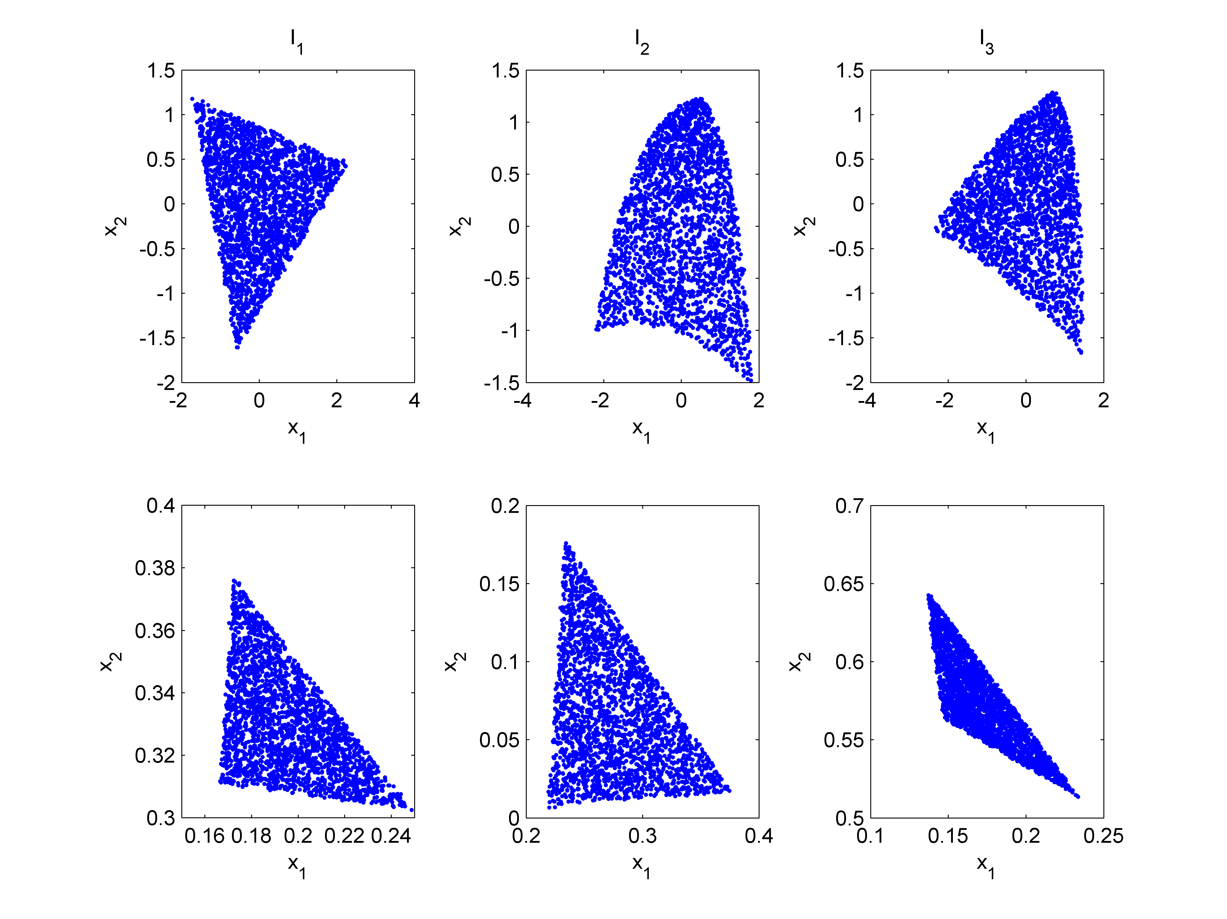
Figure 4: Top: Representation of the $N=2500$ pixels (dots) using the first two principal components provided by the standard PCA for the three synthetic images $I_{1}$ to $I_{3}$. Bottom: Representation using the latent variables estimated by the LL-GPLVM for the three synthetic images $I_{1}$ to $I_{3}$.

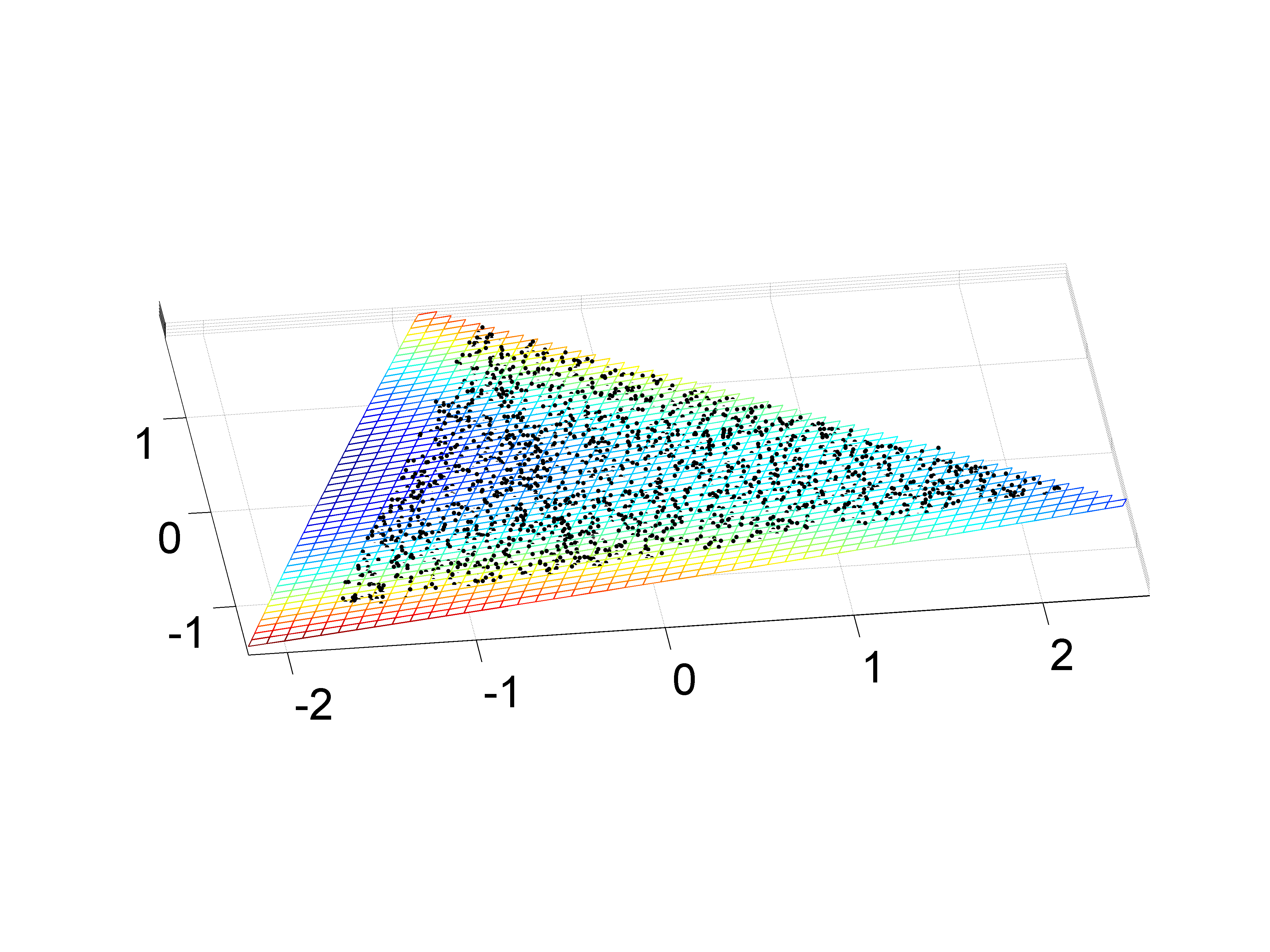
(a) $I_{1}$ (LMM)

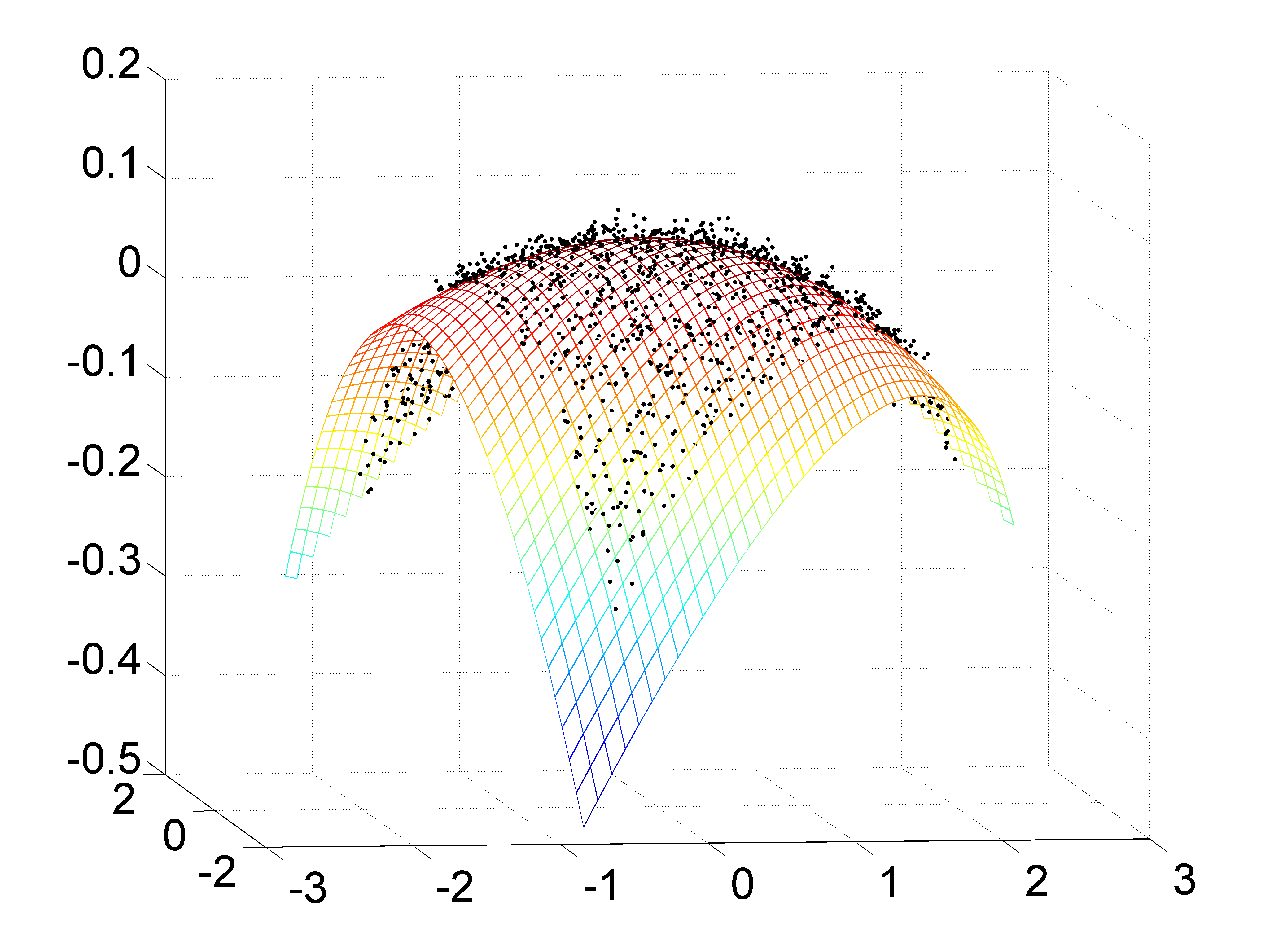
(b) $I_{2}$ (FM)

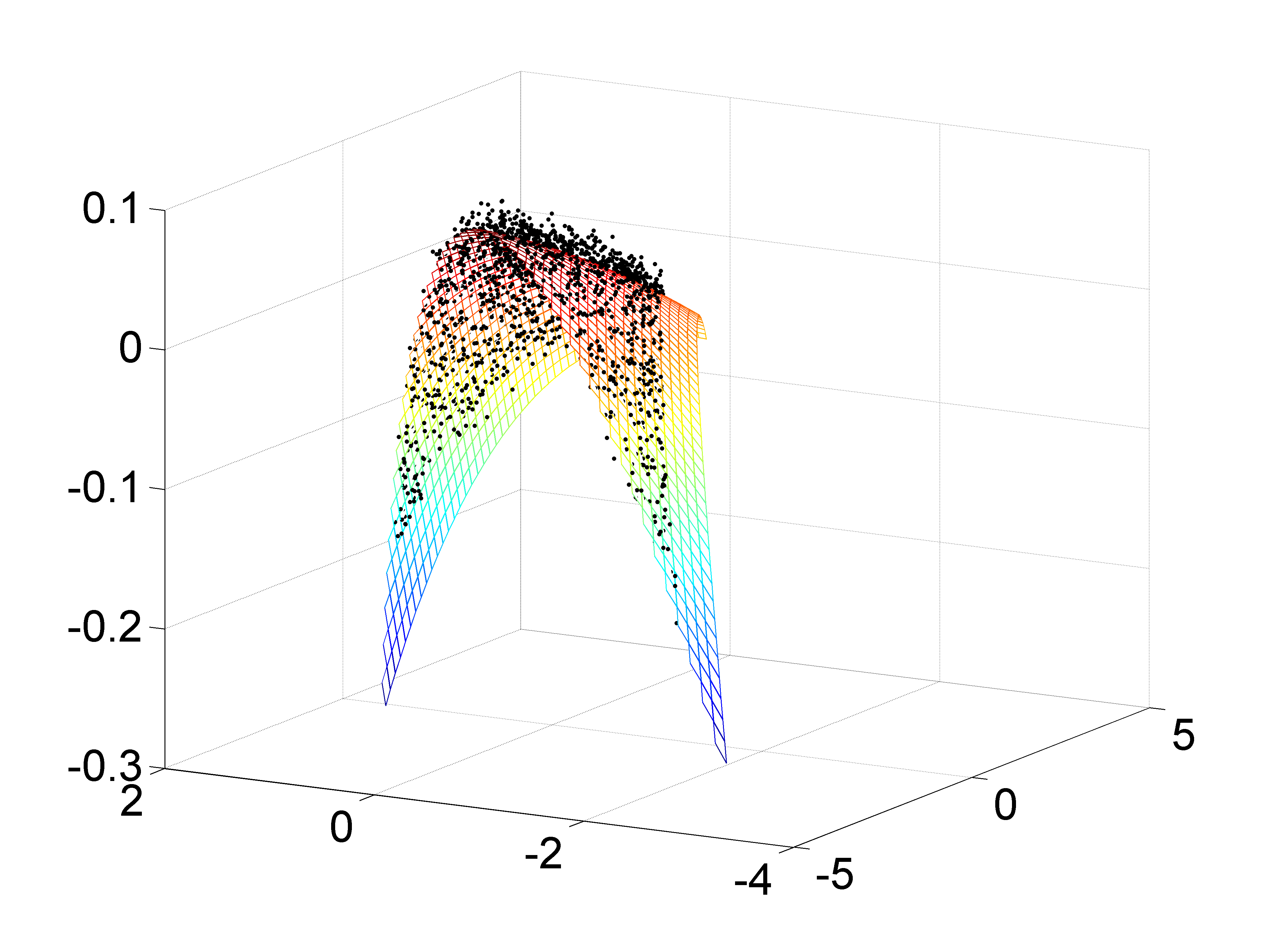
(c) $I_{3}$ (GBM)

Figure 5: Visualization of the $N=2500$ pixels (black dots) of $I_{1}$, $I_{2}$ and $I_{3}$ using the 3 axis provided by the PCA procedure. The colored surface is the manifold identified by the LL-GPLVM.

The quality of unmixing procedures can also be measured by comparing the estimated and actual abundances using the root normalized mean square error (RNMSE) defined by

$$\textrm{RNMSE}=\sqrt{\dfrac{1}{NR}\sum_{n=1}^{N}{\left\|\hat{{\boldsymbol{a}}}_{n}-{\boldsymbol{a}}_{n}\right\|^{2}}}$$ (38)

where ${\boldsymbol{a}}_{n}$ is the $n$th actual abundance vector and $\hat{{\boldsymbol{a}}}_{n}$ its estimate. Table II compares the RNMSEs obtained with different unmixing strategies. The endmembers have been estimated by the VCA algorithm in all simulations. The algorithms used for abundance estimation are the FCLS algorithm proposed in [31] for $I_{1}$, the LS method proposed in [5] for $I_{2}$ and the gradient-based method proposed in [6] for $I_{3}$. These procedures are referred to as “SU” in the table. These strategies are compared with the proposed FCLL-GPLVM. As mentioned above, the Bayesian algorithm for joint estimation of ${\mathbb{A}}$ and $\boldsymbol{V}$ under positivity and sum-to-one constraints for ${\mathbb{A}}$ (introduced in [25]) is used in this paper for the scaling step. It can be seen that the proposed FCLL-GPLVM is general enough to accurately approximate the considered mixing models since it provides the best results in term of abundance estimation.

TABLE II: RNMSEs: synthetic images.

	RNMSE ($\times 10^{-3}$)
	$I_{1}$	$I_{2}$	$I_{3}$	$I_{1}^{*}$	$I_{2}^{*}$	$I_{3}^{*}$
SU	5.7	7.4	22.7	49.3	86.6	47.8
FCLL-GPLVM	3.9	4.2	5.4	4.8	7.2	7.5

The quality of reconstruction of the unmixing procedure is also evaluated by the ARE. For the FCLL-GPLVM, the $n$th reconstructed pixel $\hat{\mathbf{y}}_{n}$ is given by $\hat{\mathbf{y}}_{n}=\widehat{\boldsymbol{P}}\widehat{\boldsymbol{U}}^{T}{\boldsymbol{\psi}}\left[\hat{\boldsymbol{x}}^{(c)}(n)\right]$. Table I also shows the AREs corresponding to the different unmixing strategies. The proposed FCLL-GPLVM outperforms the other strategies in term of ARE for these images.

Finally, the performance of the FCLL-GPLVM for endmember estimation is evaluated by comparing the estimated endmembers with the actual spectra. The quality of endmember estimation is evaluated by the spectral angle mapper (SAM) defined as

$$\textrm{SAM}=\textrm{arccos}\left(\dfrac{\left\langle\hat{{\mathbf{m}}_{r}},{\mathbf{m}}_{r}\right\rangle}{\left\|\hat{{\mathbf{m}}_{r}}\right\|\left\|{\mathbf{m}}_{r}\right\|}\right)$$ (39)

where ${\mathbf{m}}_{r}$ is the $r$th actual endmember and $\hat{{\mathbf{m}}_{r}}$ its estimate. Table III compares the SAMs obtained for each endmember using the VCA algorithm, the nonlinear EEA presented in [14] (referred to as “Heylen”) and the FCLL-GPLVM for the three images $I_{1}$ to $I_{3}$. These results show that the FCLL-GPLVM provides accurate endmember estimates for both linear and nonlinear mixtures.

TABLE III: SAMs ($\times 10^{-2}$): synthetic images.

		VCA	Heylen	FCLL-GPLVM
$I_{1}$	${\mathbf{m}}_{1}$	0.43	1.94	0.52
	${\mathbf{m}}_{2}$	0.22	0.66	0.86
	${\mathbf{m}}_{3}$	0.22	0.78	0.15
$I_{2}$	${\mathbf{m}}_{1}$	1.62	0.75	0.33
	${\mathbf{m}}_{2}$	2.08	1.69	0.53
	${\mathbf{m}}_{3}$	1.15	0.42	0.34
$I_{3}$	${\mathbf{m}}_{1}$	1.91	1.80	0.44
	${\mathbf{m}}_{2}$	1.36	0.86	0.58
	${\mathbf{m}}_{3}$	0.88	1.38	0.30

Finally, the performance of the proposed unmixing algorithm is tested in scenarios where pure pixels are not present in the observed scene. More precisely, the simulation parameters remain the same for the three images $I_{1}$ to $I_{3}$ except for the $N=2500$ abundance vectors, that are drawn from a uniform distribution in the following set

$$\left\{{\boldsymbol{a}}\big{|}\sum_{r=1}^{R}{a_{r}}=1,~{}~{}0.9\geq a_{r}(n)\geq 0,\forall r\in\left\{1,\ldots,R\right\}\right\}.$$ (40)

The three resulting images are denoted as $I_{1}^{*}$, $I_{2}^{*}$ and $I_{3}^{*}$. Table I shows that the absence of pure pixels does not change the AREs significantly when they are compared with those obtained with the images $I_{1}$ to $I_{3}$. Moreover, FCLL-GPLVM is more robust to the absence of pure pixels than the different SU methods. The good performance of FCLL-GPVLM is due in part to the scaling procedure. Table II shows that the performance of the FCLL-GPLVM in term of RNMSE is not degraded significantly when there is no pure pixel in the image (note that the situation is different when the endmembers are estimated using VCA). Table IV shows the performance of the FCLL-GPLVM for endmember estimation when there are no pure pixels in the image. The results of the FCLL-GPLVM do not change significantly when they are compared with those obtained with images $I_{1}$ to $I_{3}$, which is not the case for the two other EEAs. The accuracy of the endmember estimation is illustrated in Fig. 6 which compares the endmembers estimated by the FCLL-GPLVM (blue lines) to the actual endmember (red dots) and the VCA estimates (black line) for the image $I_{2}^{*}$.

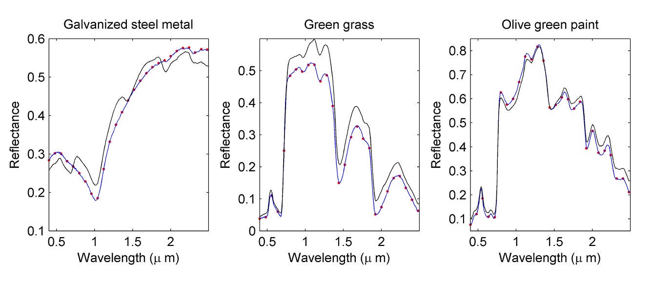
Figure 6: Actual endmembers (red dots) and endmembers estimated by the FCLL-GPLVM (blue lines) and VCA (black line) for the image $I_{2}^{*}$.

The next section presents simulation results obtained for real data.

TABLE IV: SAMs ($\times 10^{-2}$): synthetic images.

		VCA	Heylen	FCLL-GPLVM
$I_{1}^{*}$	${\mathbf{m}}_{1}$	2.87	6.38	0.38
	${\mathbf{m}}_{2}$	2.15	11.11	1.30
	${\mathbf{m}}_{3}$	2.10	2.62	0.24
$I_{2}^{*}$	${\mathbf{m}}_{1}$	5.22	7.53	0.67
	${\mathbf{m}}_{2}$	8.02	9.59	1.46
	${\mathbf{m}}_{3}$	7.10	2.48	0.53
$I_{3}^{*}$	${\mathbf{m}}_{1}$	6.89	6.59	0.61
	${\mathbf{m}}_{2}$	6.03	5.95	1.75
	${\mathbf{m}}_{3}$	3.73	2.36	0.48

VI-B Real data

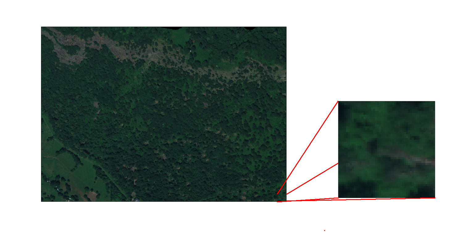
Figure 7: Real hyperspectral data: Madonna data acquired by the Hyspex hyperspectral scanner over Villelongue, France (left) and the region of interest shown in true colors (right).

The real image considered in this section was acquired in 2010 by the Hyspex hyperspectral scanner over Villelongue, France. $L=160$ spectral bands were recorded from the visible to near infrared with a spatial resolution of $0.5$m. This dataset has already been studied in [32] and is mainly composed of different vegetation species. The sub-image of size $50\times 50$ pixels chosen here to evaluate the proposed unmixing procedure is depicted in Fig. 7. This image is mainly composed of three components since the data belong to a two-dimensional manifold (see black dots of Fig. 8 (a)). Consequently, we assume that the scene is composed of $R=3$ endmembers. Using the ground truth used in [32], we can determine some tree species present in the scene of interest. More precisely, Fig. 8 (a) shows the ground truth clusters corresponding to oak trees (red dots) and chestnut trees (blue dots) projected in a 3-dimensional subspace (defined by the first three principal components of a PCA applied to the image of Fig. 7). These two clusters are close to vertices of the data cloud. Consequently, oak and chestnut trees are identified as endmembers present in the image. Moreover, the third endmember is not a tree species according to the ground truth provided in [32]. In the sequel, this endmember will be referred to as Endmember $\sharp 3$.

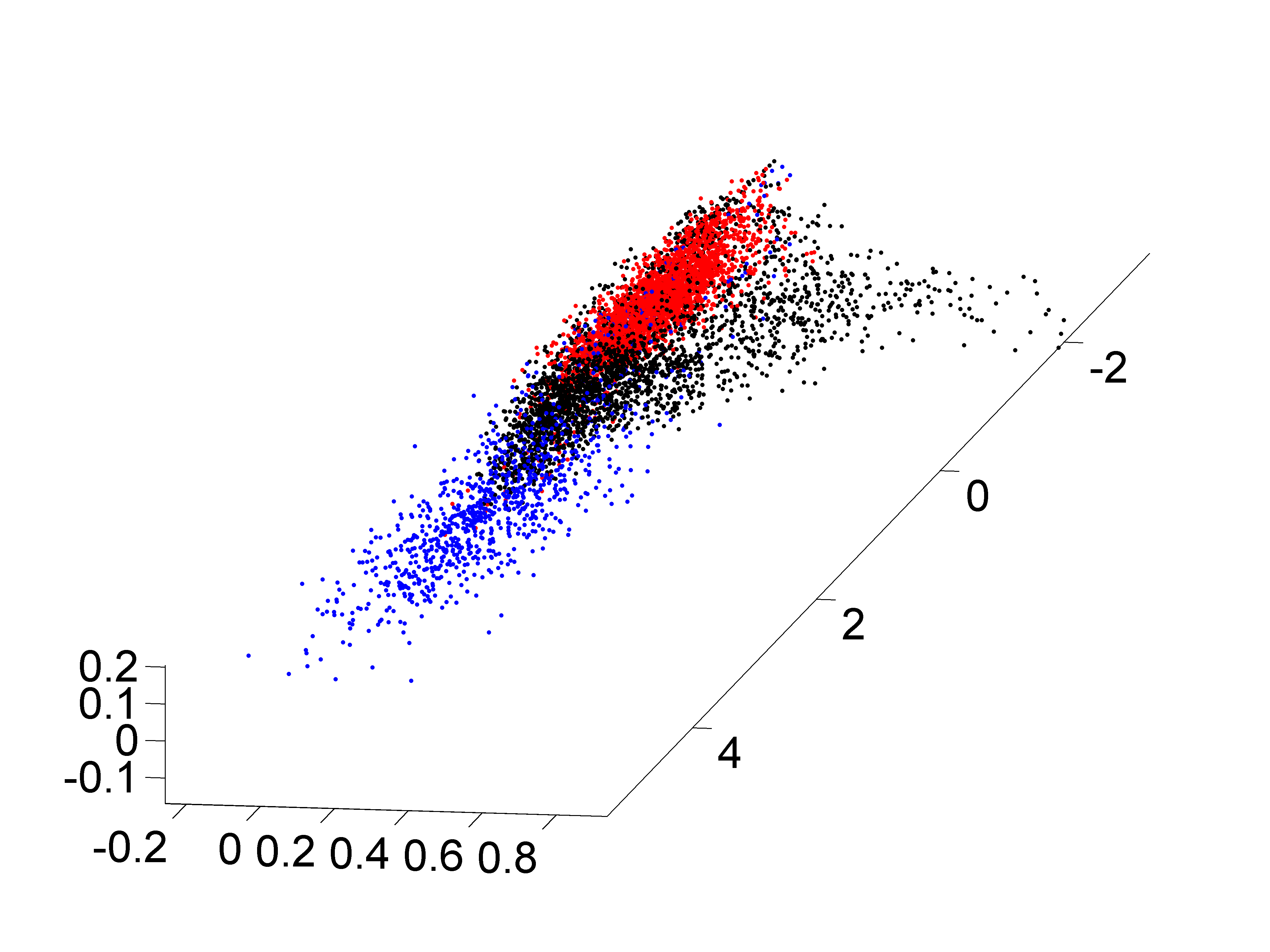
(a)

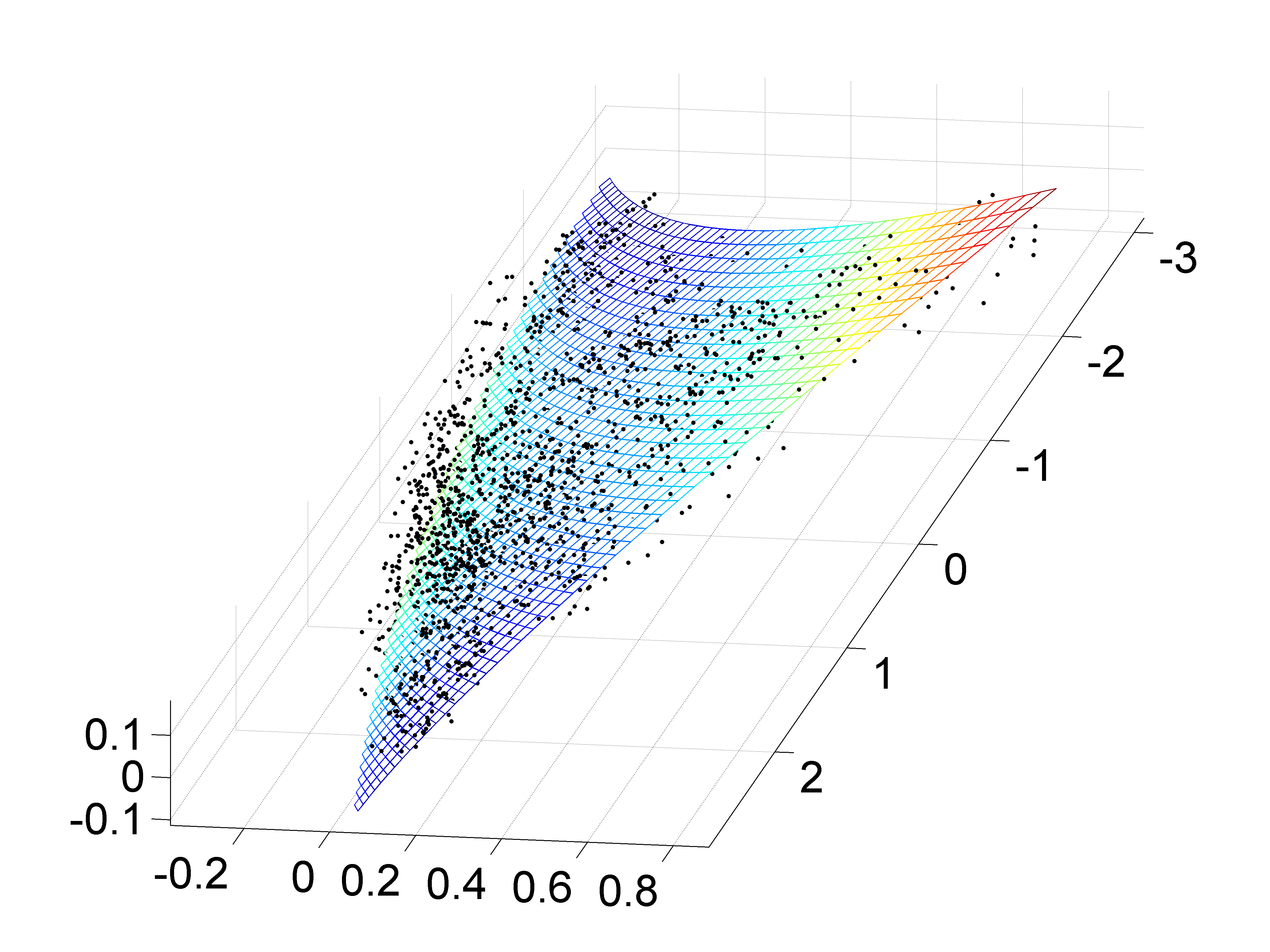
(b)

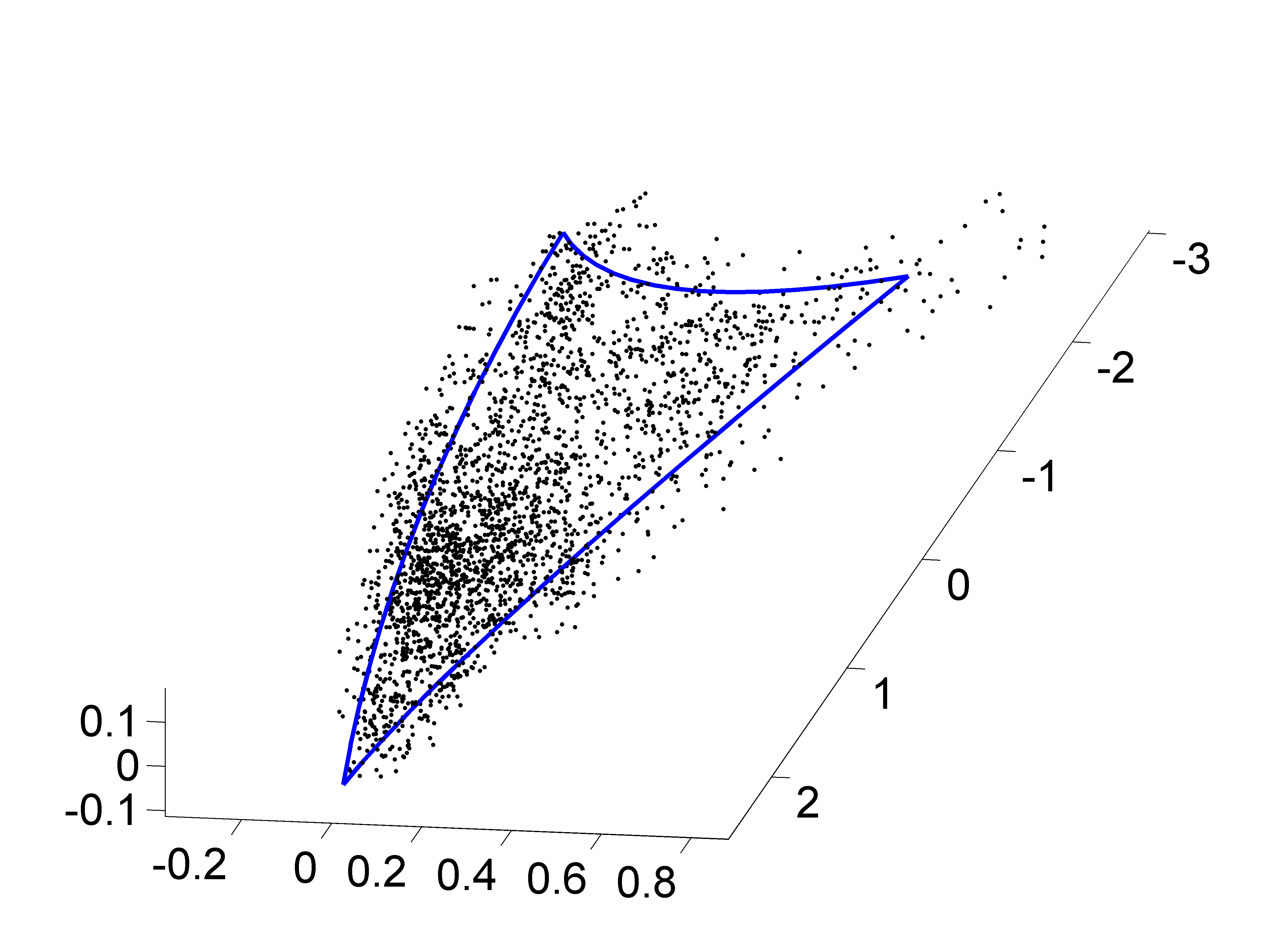
(c)

Figure 8: (a): Representation of the $N=2500$ pixels (black dots) of the Madonna image and the ground truth clusters corresponding to oak trees (red dots) and chestnut trees (blue dots) using the first three principal components provided by the standard PCA. (b): Representation of the $N=2500$ pixels (dots) of the Madonna data and manifold identified by the LL-GPLVM (colored surface). (c):Representation of the $N=2500$ pixels (dots) of the Madonna data and boundaries of the estimated transformed simplex (blue lines).

The simulation parameters have been fixed to $\gamma=10^{3}$ and $K=R$. The latent variables obtained by maximizing the marginalized posterior distribution (10) are depicted in Fig. 9 (blue dots).

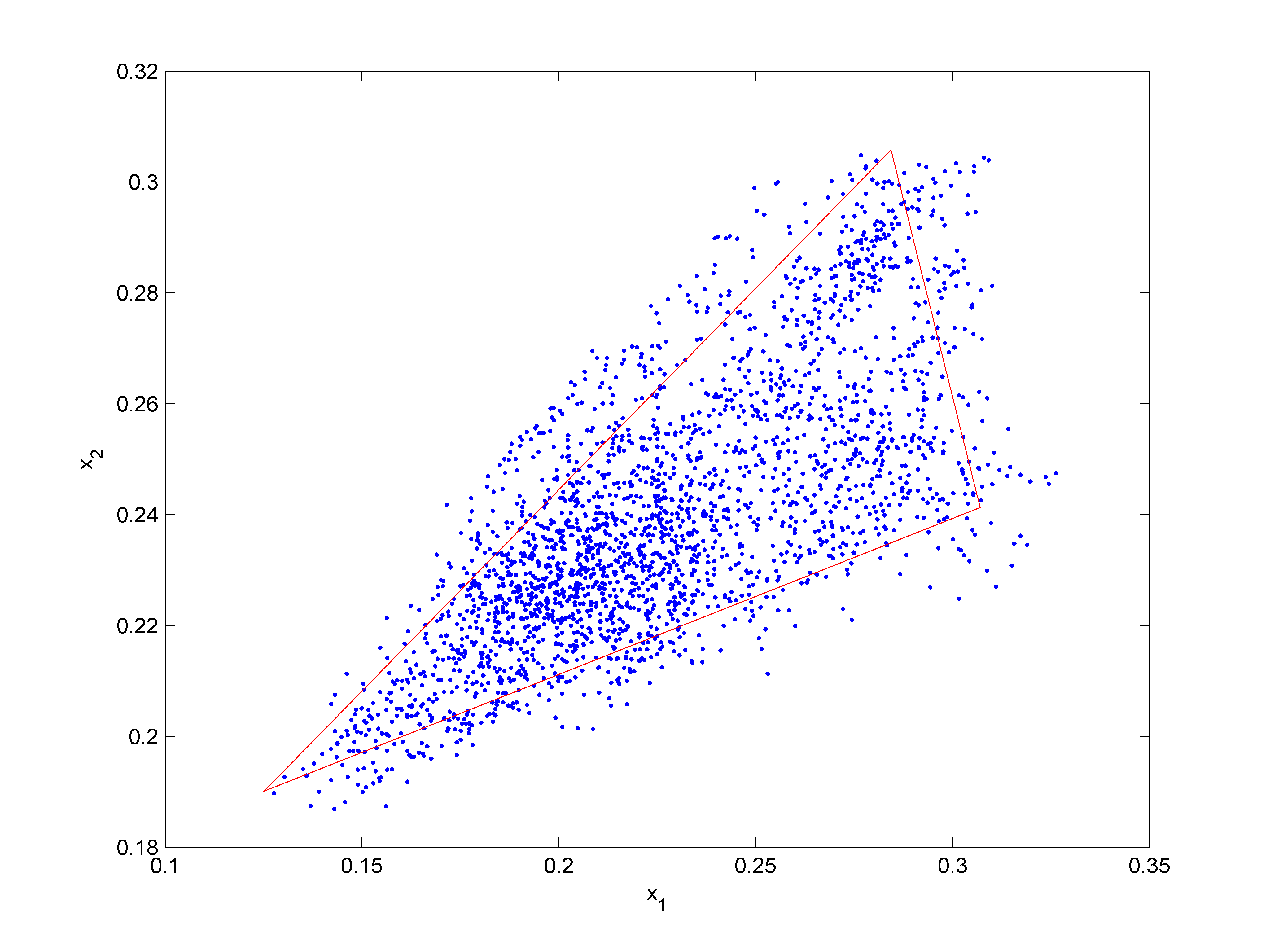
Figure 9: Representation of the $N=2500$ latent variables (dots) estimated by the LL-GPLVM and the simplex identified by the scaling step (red lines) for the Madonna data.

It can be seen from this figure that the latent variables seem to describe a noisy simplex. Fig. 8 (b) shows the manifold estimated by the proposed LL-GPLVM. This figure illustrates the capacity of the LL-GPLVM for modeling the nonlinear manifold. Table V (left) compares the AREs obtained by the proposed LL-GPLVM and the projection onto the first $R-1=2$ principal vectors provided by PCA. The proposed LL-GPLVM slightly outperforms PCA for the real data of interest, which shows that the proposed nonlinear dimensionality reduction method is more accurate than PCA (linear dimensionality reduction) in representing the data. The scaling step presented in Section IV is then applied to the estimated latent variables. The estimated simplex defined by the latent variables is depicted in Fig. 9 (red lines). Fig. 8 (c) compares the boundaries of the estimated transformed simplex with the image pixels. The abundance maps obtained after the scaling step are shown in Fig. 10 (top). The results of the unmixing procedure using the FCLL-GPLVM are compared to an unmixing strategy assuming the LMM. More precisely, we use VCA to extract the endmembers from the data and use the FLCS algorithm for abundance estimation. The estimated abundance maps are depicted in Fig. 10 (bottom). The abundance maps obtained by the two methods are similar which shows the accuracy of the proposed unmixing strategy when considering the LMM as a first order approximation of the mixing model.

TABLE V: AREs: real image ($\times 10^{-2}$).

PCA	LL-GPLVM	VCA+FCLS	FCLL-GPLVM
0.84	0.79	1.30	1.11

Moreover, Fig. 11 shows the classification map obtained in [32] for the region of interest. The unclassified pixels correspond to areas where the classification method of [32] has not been performed. Even if lots of pixels are not classified, the classified pixels can be compared with the estimated abundance maps. First, we can note the presence of the same tree species in the classification and abundance maps, i.e., oak and chestnut. We can also see that the pixels composed of chestnut trees and Endmember $\sharp 3$ are mainly located in the unclassified regions, which explains why they do not appear clearly in the classification map. Only one pixel is classified as being composed of ash trees in the region of interest. If unclassified pixels also contain ash trees, they are either too few or too mixed to be considered as mixtures of an additional endmember in the image. Finally, it can be seen from Figs. 10 and 11 that oak trees are located within similar regions (left corners and top right corner) for the abundance and classification maps.

Evaluating the performance of endmember estimation on real data is an interesting problem. However, comparison of the estimated endmembers with the ground truth is difficult here. First, since the nature of Endmember $\sharp 3$ is unknown, no ground truth is available for this endmember. Second, because of the variability of the ground truth spectra associated with each tree species, it is difficult to show whether VCA or the proposed FCLL-GPLVM provides the best endmember estimates. However, the AREs obtained for both methods (Table V, right) show that the FCLL-GPLVM fits the data better than the linear SU strategy, which confirms the importance of the proposed algorithm for nonlinear spectral unmixing.

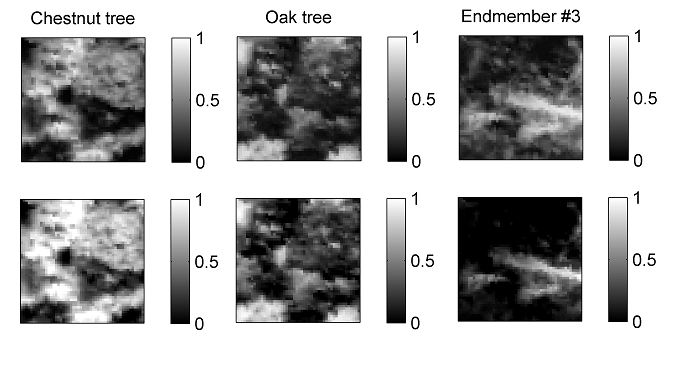
Figure 10: Top: Abundance maps estimated using the FCLL-GPLVM for the Madonna image. Bottom: Abundance maps estimated using the VCA algorithm for endmember extraction and the FCLS algorithm for abundance estimation.

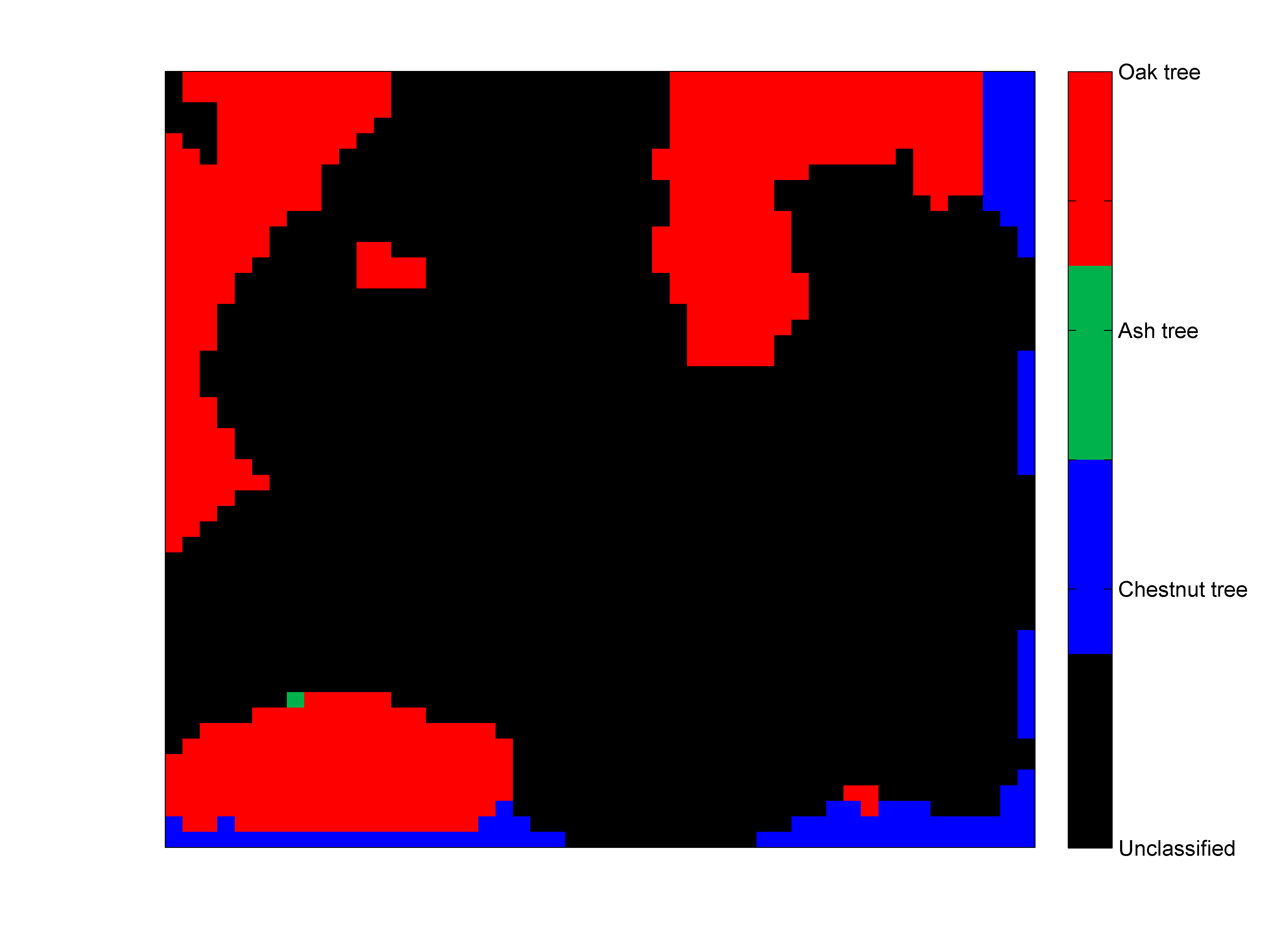
Figure 11: Classification map obtained in [32] for the region of interest of the Madonna image.

VII Conclusions

We proposed a new algorithm for nonlinear spectral unmixing based on a Gaussian process latent variable model. The unmixing procedure assumed a nonlinear mapping from the abundance space to the observed pixels. It also considered the physical constraints for the abundance vectors. The abundance estimation was decomposed into two steps. Dimensionality reduction was first achieved using latent variables. A scaling procedure was then proposed to estimate the abundances. After estimating the abundance vectors of the image, a new endmember estimator based on Gaussian process regression was investigated. Simulations conducted on synthetic and real images illustrated the flexibility of the proposed model for linear and nonlinear spectral unmixing and provided promising results for abundance and endmember estimations in spite of the absence of pure pixels in the image. The choice of the nonlinear mapping used for the GP model is an important issue to ensure that the LL-GPLVM is general enough to handle different nonlinearities. In particular, different mappings could be used for intimate mixtures. Moreover, including the GPLVM in a Bayesian framework could also be an interesting prospect to consider spatial correlation through Markov random fields or GPs.

References

- [1] J. M. Bioucas-Dias, A. Plaza, N. Dobigeon, M. Parente, Q. Du, P. Gader, and J. Chanussot, “Hyperspectral unmixing overview: Geometrical, statistical, and sparse regression-based approaches,” IEEE J. Sel. Topics Appl. Earth Observations Remote Sensing, vol. 5, no. 2, pp. 354–379, April 2012.
- [2] B. W. Hapke, “Bidirectional reflectance spectroscopy. I. Theory,” J. Geophys. Res., vol. 86, pp. 3039– 3054, 1981.
- [3] B. Somers, K. Cools, S. Delalieux, J. Stuckens, D. V. der Zande, W. W. Verstraeten, and P. Coppin, “Nonlinear hyperspectral mixture analysis for tree cover estimates in orchards,” Remote Sensing of Environment, vol. 113, no. 6, pp. 1183–1193, 2009.
- [4] J. M. P. Nascimento and J. M. Bioucas-Dias, “Nonlinear mixture model for hyperspectral unmixing,” Proc. of the SPIE, vol. 7477, pp. 74 770I–74 770I–8, 2009.
- [5] W. Fan, B. Hu, J. Miller, and M. Li, “Comparative study between a new nonlinear model and common linear model for analysing laboratory simulated-forest hyperspectral data,” Remote Sensing of Environment, vol. 30, no. 11, pp. 2951–2962, June 2009.
- [6] A. Halimi, Y. Altmann, N. Dobigeon, and J.-Y. Tourneret, “Nonlinear unmixing of hyperspectral images using a generalized bilinear model,” IEEE Trans. Geosci. and Remote Sensing, vol. 49, no. 11, pp. 4153–4162, Nov. 2011.
- [7] K. J. Guilfoyle, M. L. Althouse, and C.-I. Chang, “A quantitative and comparative analysis of linear and nonlinear spectral mixture models using radial basis function neural networks,” IEEE Geosci. and Remote Sensing Lett., vol. 39, no. 8, pp. 2314–2318, Aug. 2001.
- [8] Y. Altmann, N. Dobigeon, S. McLaughlin, and J.-Y. Tourneret, “Nonlinear unmixing of hyperspectral images using radial basis functions and orthogonal least squares,” in Proc. IEEE Int. Conf. Geosci. and Remote Sensing (IGARSS), July 2011, pp. 1151–1154.
- [9] Y. Altmann, A. Halimi, N. Dobigeon, and J.-Y. Tourneret, “Supervised nonlinear spectral unmixing using a postnonlinear mixing model for hyperspectral imagery,” IEEE Trans. Image Processing, vol. 21, no. 6, pp. 3017–3025, 2012.
- [10] J. Broadwater, R. Chellappa, A. Banerjee, and P. Burlina, “Kernel fully constrained least squares abundance estimates,” in Proc. IEEE Int. Conf. Geosci. and Remote Sensing (IGARSS), July 2007, pp. 4041–4044.
- [11] K.-H. Liu, E. Wong, and C.-I. Chang, “Kernel-based linear spectral mixture analysis for hyperspectral image classification,” in Proc. IEEE GRSS Workshop on Hyperspectral Image and Signal Processing: Evolution in Remote Sensing (WHISPERS), Aug. 2009, pp. 1–4.
- [12] J. Chen, C. Richard, and P. Honeine, “A novel kernel-based nonlinear unmixing scheme of hyperspectral images,” in Asilomar Conf. Signals, Systems, Computers, Nov. 2011, pp. 1898–1902.
- [13] ——, “Nonlinear unmixing of hyperspectral data based on a linear-mixture/nonlinear-fluctuation model,” IEEE Trans. Signal Process., 2012, submitted.
- [14] R. Heylen, D. Burazerovic, and P. Scheunders, “Non-linear spectral unmixing by geodesic simplex volume maximization,” IEEE Journal of Selected Topics in Signal Processing, vol. 5, no. 3, pp. 534–542, June 2011.
- [15] N. D. Lawrence, “Gaussian process latent variable models for visualisation of high dimensional data,” in NIPS, Vancouver, Canada, 2003.
- [16] E. V. Bonilla, F. V. Agakov, and C. K. I. Williams, “Kernel multi-task learning using task-specific features,” in Proc. of the 11th Int. Conf. on Artificial Intelligence and Statistics (AISTATS), 2007.
- [17] M. A. Alvarez, L. Rosasco, and N. D. Lawrence, “Kernels for Vector-Valued Functions: a Review,” June 2011. [Online]. Available: http://arxiv.org/abs/1106.6251
- [18] Y. Altmann, N. Dobigeon, S. McLaughlin, and J.-Y. Tourneret, “Nonlinear spectral unmixing of hyperspectral images using gaussian processes,” University of Toulouse, France, Tech. Rep., July 2012. [Online]. Available: http://altmann.perso.enseeiht.fr/
- [19] J. Qui onero-candela, C. E. Rasmussen, and R. Herbrich, “A unifying view of sparse approximate Gaussian process regression,” Journal of Machine Learning Research, vol. 6, p. 2005, 2005.
- [20] N. D. Lawrence, “The Gaussian process latent variable model,” University of Sheffield, Department of Computer Science, Tech. Rep., Jan. 2006. [Online]. Available: http://staffwww.dcs.shef.ac.uk/people/N.Lawrence/
- [21] J. Wang and C.-I Chang, “Applications of independent component analysis in endmember extraction and abundance quantification for hyperspectral imagery,” IEEE Trans. Geosci. and Remote Sensing, vol. 4, no. 9, pp. 2601–2616, Sept. 2006.
- [22] R. Urtasun, D. J. Fleet, and N. D. Lawrence, “Modeling human locomotion with topologically constrained latent variable models,” in Conf. Human motion: understanding, modeling, capture and animation. Rio de Janeiro, Brazil: Springer-Verlag, 2007, pp. 104–118.
- [23] C. E. Rasmussen and C. K. I. Williams, Gaussian Processes for Machine Learning (Adaptive Computation and Machine Learning). The MIT Press, 2005.
- [24] M. Brookes, The Matrix Reference Manual, Imperial College, London, UK, 2005.
- [25] N. Dobigeon, S. Moussaoui, M. Coulon, J.-Y. Tourneret, and A. O. Hero, “Joint Bayesian endmember extraction and linear unmixing for hyperspectral imagery,” IEEE Trans. Signal Process., vol. 57, no. 11, pp. 2657–2669, Nov. 2009.
- [26] F. Chaudhry, C.-C. Wu, W. Liu, C.-I Chang, and A. Plaza, “Pixel purity index-based algorithms for endmember extraction from hyperspectral imagery,” in Recent Advances in Hyperspectral Signal and Image Processing, C.-I Chang, Ed. Trivandrum, Kerala, India: Research Signpost, 2006, ch. 2.
- [27] M. Winter, “Fast autonomous spectral end-member determination in hyperspectral data,” in Proc. 13th Int. Conf. on Applied Geologic Remote Sensing, vol. 2, Vancouver, April 1999, pp. 337–344.
- [28] J. M. P. Nascimento and J. M. Bioucas-Dias, “Vertex component analysis: A fast algorithm to unmix hyperspectral data,” IEEE Trans. Geosci. and Remote Sensing, vol. 43, no. 4, pp. 898–910, April 2005.
- [29] J. Li and J. M. Bioucas-Dias, “Minimum volume simplex analysis: a fast algorithm to unmix hyperspectral data,” in Proc. IEEE Int. Conf. Geosci. and Remote Sensing (IGARSS), vol. 3, Boston, USA, July 2008, pp. 250–253.
- [30] RSI (Research Systems Inc.), ENVI User’s guide Version 4.0, Boulder, CO 80301 USA, Sept. 2003.
- [31] D. C. Heinz and C.-I Chang, “Fully constrained least-squares linear spectral mixture analysis method for material quantification in hyperspectral imagery,” IEEE Trans. Geosci. and Remote Sensing, vol. 29, no. 3, pp. 529–545, March 2001.
- [32] D. Sheeren, M. Fauvel, S. Ladet, A. Jacquin, G. Bertoni, and A. Gibon, “Mapping ash tree colonization in an agricultural mountain landscape: Investigating the potential of hyperspectral imagery,” in Proc. IEEE Int. Conf. Geosci. and Remote Sensing (IGARSS), July 2011, pp. 3672–3675.