Turbulence induced collisional velocities and density enhancements: large inertial range results from shell models

Abstract

To understand the earliest stages of planet formation, it is crucial to be able to predict the rate and the outcome of dust grains collisions, be it sticking and growth, bouncing, or fragmentation. The outcome of such collisions depends on the collision speed, so we need a solid understanding of the rate and velocity distribution of turbulence-induced dust grain collisions. The rate of the collisions depends both on the speed of the collisions and the degree of clustering experienced by the dust grains, which is a known outcome of turbulence. We evolve the motion of dust grains in simulated turbulence, an approach that allows a large turbulent inertial range making it possible to investigate the effect of turbulence on meso-scale grains (millimeter and centimeter). We find three populations of dust grains: one highly clustered, cold and collisionless; one warm; and the third “hot”. Our results can be fit by a simple formula, and predict both significantly slower typical collisional velocities for a given turbulent strength than previously considered, and modest effective clustering of the collisional populations, easing difficulties associated with bouncing and fragmentation barriers to dust grain growth. Nonetheless, the rate of high velocity collisions falls off merely exponentially with relative velocity so some mid- or high-velocity collisions will still occur, promising some fragmentation.

1. Introduction

Collisions between dust grains in protoplanetary disks is a key process in planetesimal formation, and so has seen a significant amount of study, both theoretical (Völk et al., 1980; Markiewicz et al., 1991; Cuzzi & Hogan, 2003; Youdin & Goodman, 2005; Ormel & Cuzzi, 2007) and numerical (Dullemond & Dominik, 2005; Johansen et al., 2007). More, the results of collisions between artificial dust grains as a function of relative velocity can be directly observed in laboratory experiments (Blum & Wurm, 2008; Güttler et al., 2010). These collisions can lead to sticking and growth of dust grains, or to fragmentation, repopulating the smallest sizes of dust grains. On the other hand, laboratory experiments suggest that the null-result of a collision, bouncing, poses a significant threat to dust growth beyond the cm scale (Zsom et al., 2010).

The gas component of protoplanetary disks is believed to be turbulent, and the effect of this turbulence on the collisions between dust particles entrained in the flow can be reasonably estimated analytically, for example as done in the line of work starting with Völk et al. (1980) and more recently elaborated on by Ormel & Cuzzi (2007). Such analyses give the unsurprising result that dust collisional velocities are comparable to the turbulent velocities of the gas on scales set by the properties of the dust grains. These estimated velocities are, however, expected to be large. The turbulence in protoplanetary disks is often invoked to explain the disk’s accretion on the mega-year time-scales observed (Shakura & Sunyaev, 1973; Russell et al., 2006), and the turbulent motions required to achieve such a feat are expected to drive dust collisions that destroy the participants or merely result in bouncing (Wurm et al., 2001; Güttler et al., 2010; Wettlaufer, 2010). The existence of the bouncing and fragmentation velocity cut-offs means that it is important to determine not merely the rate of collisions, but also the collisional probability distribution as a function of the relative velocity, because outlying events could cross the bouncing barrier (Zsom et al., 2010).

Another important behavior of particles in turbulence is “preferential concentration” (Maxey, 1987; Fessler et al., 1994; Cuzzi et al., 2001; Toschi & Bodenschatz, 2009), where inertial particles are ejected from regions of high vorticity due to centrifugal forces, and accumulate in regions of high strain. This has been hypothesized to increase dust collision rates by creating local dust density fluctuations (Pan et al., 2011), as well as possibly leading to dust drag on the turbulence. The latter can cause a streaming-instability that further enhances the local dust density (Youdin & Goodman, 2005; Johansen et al., 2007). Beyond the effect on dust grain collisions rates, such density enhancements can provide a rapid route to gravitational instabilities and the resulting collapse into planetesimals (Johansen et al., 2006). This ejection of inertial particles from turbulent (intermittent) vorticies, which will be discussed in this paper, should be distinguished from the dust-trapping property of anti-cyclonic long-lived vortices, which are large enough to feel Coriolis forces (Barge & Sommeria, 1995; Johansen et al., 2004).

Moreover, the inertial range of the turbulence in these systems is expected to be quite broad, easily five to six orders of magnitude in k-space or four orders of magnitude in turbulent turn-over time, as their fluid Reynolds numbers are large. This means that there will be dust grains well embedded in the turbulent cascade, too small to notice that they are trapped within huge eddies, yet too large to be meaningfully affected by the smallest scale turbulence. These well embedded particles are precisely the most important ones, since they include the millimeter–centimeter sized dust grains that populate the fragmentation and bouncing barriers. A resolution on the order of several thousand cubed would be required to fully simulate a system evolving the full Navier-Stokes equations with an upper double digit inertial range, beyond currently available resources. Further, as we will show, turbulent clustering implies that very small particle separations must be considered to extract useful data. The resolution required for performing a full hydrodynamical simulation is, again, on the order of several thousand cubed (Section 4.1).

Carballido et al. (2010) explicitly run into the above-mentioned problems of limited inertial range and low spatial resolution. We resolve these problems by putting particles into a set of turbulent cascade models known as shell models (Bohr et al. 1998, chapter 3), which allows us determine the clustering and collisional velocity probability distributions that can be expected for large inertial ranges (up to $256$) while resolving small particle separations. This approach of using synthetic turbulence was also used by Bec et al. (2005), although the details of the projection into real space differs. Our work also differs by our focus on the collisional velocities as a key diagnostic, and we find noticeably lower collisional velocities than those estimated analytically by Völk et al. (1980) and following. Further, unlike those works, our results are not well approximated by a single effective collisional velocity, but require consideration of a velocity probability distribution. While our clustering results are similar to those of Pan et al. (2011), simultaneously considering the collisional velocities allows us to distinguish between multiple particle collisional populations, which changes the conclusions about the effects of the strong clustering that is observed.

In Section 2 we define our numerical methods and in Section 3 we use them to investigate a particular base case to find the physical behavior. In Section 4 we investigate systems with different inertial ranges and synthetic turbulence implementations. We compare our results with previous work in Section 5 and conclude in Section 6. We list our main variables, parameters, and diagnostics in Table 4 and discuss the definition and use of the Stokes number in Appendix A.

2. Numerical setup

We use the Pencil Code to track the motion of particles in synthetic turbulent cascades. Our synthetic turbulence derives from shell models: we consider spatial Fourier transforms of the turbulent velocity field (from $\bm{x}$ to $\bm{k}$), keeping the modes that fit in a limited range of $|\bm{k}|$ which defines our considered subsection of the inertial range. We then coarse-grain the sphere of $\bm{k}$ vectors into logarithmically spaced shells in $k$-space. As such, we consider only the energy spectrum of the turbulence. We will use four different models. Three follow an exact Kolmogorov power spectrum (Kolmogorov 1941, see Section 2.1) and differ only in the implementation of their time variability, if any. The fourth model, discussed in Section 2.1.1, combines the spatial approach of Section 2.1 with an energy spectrum derived from a GOY model, which solves a set of equations for the turbulent energy cascade. However, it should be noted that the magnitude of the velocity field in a GOY model is strongly fluctuating in time, making the choice of dimensionless quantities less obvious. A first study with a time-independent energy spectrum is needed to establish the form of turbulent collisional velocities and is closer to existing analytical work.

Since we do not evolve the Navier-Stokes equations to determine the gas motion, we do not need a grid or a sub-grid model: this allows for greater resolution. We evolve $4\times 10^{6}$ particles in a periodic box of size $(2\pi)^{3}$. Our setup does not allow for the study of dust backreaction on turbulence (preventing, for example, the streaming instability), but does allow us to examine dust pairs at very small relative separation.

2.1. Flow field

Each coarse-grained shell is associated with a fluid velocity and turnover time and indexed with $m$ which runs from $m_{\text{min}}$ to $m_{\text{max}}$ with

$$k_{m}=2^{m},$$ (1)

$$\tau_{m}=1/v_{m}k_{m}.$$ (2)

In a Kolmogorov spectrum, the velocity obeys the power-wave

$$v_{m}=v_{0}k_{m}^{-1/3};\\$$ (3)

this generates the dashed/red velocity spectrum in Figure 1 by construction. Our choice of $m_{\text{min}}$ and $m_{\text{max}}$ is limited by available numerical resources and by the constraints of the periodicity of the numerical box. We will vary them for different simulations as the choice determines the effective inertial range of our turbulence-simulate. This allows us to find the effective inertial range large enough that the particle response becomes scale free (Appendix A).

While Equation (3) defines the amplitude of the velocity on spatial scales $k^{-1}$, we need an actual velocity field to evolve our particle positions. To obtain it, we associate each shell $m$ with three $(\bm{k}_{mn},\hat{\mbox{\boldmath$v$}{}}_{mn})$ vector pairs indexed by $n$. These vector pairs characterize contributions to the gas velocity directed along $\hat{\mbox{\boldmath$v$}{}}_{mn}$, and varying along $\bm{k}_{mn}$ (for shell $m$, $|\bm{k}|=k_{m}$). We impose $\bm{k}_{mn}\perp\hat{\mbox{\boldmath$v$}{}}_{mn}$, so that the flow is incompressible. Further, the $\bm{k}_{mi}$ and $\hat{\mbox{\boldmath$v$}{}}_{mi}$ vectors for pair $i$ of shell $m$ are approximately perpendicular to their counterparts in the other two pairs of that shell. This formulation (3 quasi-perpendicular vectors for both $\bm{k}$ and $\hat{\mbox{\boldmath$v$}{}}$ for each shell in $k$-space) allows us to span both $k$-space and velocity space in each shell separately while simultaneously avoiding strongly preferred directions. The projection of the velocity $v_{m}$ associated with shell $m$ onto the three vector pairs is done through the introduction of a unit vector $\mbox{\boldmath$a$}{}_{m}$. The three components of $\mbox{\boldmath$a$}{}_{m}$ define the relative excitation of the three possible vector pairs.

The gas velocity is then given by

$$\bm{V}(\bm{x},t) =\Sigma_{m=m_{\text{min}}}^{m_{\text{max}}}\Sigma_{n=1}^{3}$$

$$2^{1/2}a_{mn}(t)v_{m}\hat{\mbox{\boldmath$v$}{}}_{mn}\cos[\bm{k}_{mn}\cdot\bm{x}+\phi_{mn}(t)],$$ (4)

where the outer sum is over shells in $k$-space, the inner sum is over the trio of ($\bm{k}$,$\hat{\mbox{\boldmath$v$}{}}$) vector pairs, and $\phi_{mn}$ is a phase shift included to avoid overlap at $\bm{x}=0$. Note that $a_{mn}$ is a scalar (the n-th component of $\mbox{\boldmath$a$}{}_{m}$, itself a unit vector) while $\hat{\mbox{\boldmath$v$}{}}_{mn}$ is the $n$th unit vector associated with the $m$th shell. Time dependence of the flow is allowed in three ways. First, the projection onto the $\bm{k}$ and $\hat{\mbox{\boldmath$v$}{}}$ vectors can be quenched ($\mbox{\boldmath$a$}{}_{m}$ and $\phi_{mn}$ held constant); these runs are named with a “Q”. Second, we can vary the unit vectors $\mbox{\boldmath$a$}{}_{m}$ for each shell through a random walk on timescales $\tau_{m}$, with $\phi_{mn}$ held constant. This is our default method, with runs denoted by a “B”. Third, we allow the various phases $\phi_{mn}$ to vary as random walks while the $\mbox{\boldmath$a$}{}_{m}$ vectors are held constant in time; these runs are named with a “P”. Note that the GOY model inherently includes phase variation by evolving a complex value for $v_{m}$ (see Section 2.1.1).

We will use the subscripts $ls$ (large scale) for $m_{\text{min}}$ and $ss$ (small scale) for $m_{\text{max}}$. This approach of using an artificial velocity field is similar to that of Bec et al. (2005). Our prescription is closer to that used in previous analytical studies. It does however limit us to only considering turbulence in the inertial range as we have no means of tracking behavior and the energy injection or viscous dissipation scales.

Our box size is $L=2\pi$ and our boundary conditions are periodic, so the minimal $k$ is $k=1$ ($m=0$). The largest $k$ we will consider is $k=256$ ($m=8$). In practical terms, assuming an energy-carrying scale at $k=4$ and a dissipative scale at a quarter of the Nyquist wave number one would require approximately $8000^{3}$ grid points to directly simulate the turbulence for our largest inertial range (as compared to the very high resolution of $2048^{3}$ in Bec et al. 2010a). The benefit here can be seen in Figure 1 of Carballido et al. (2010), where the inertial range is, perhaps, $10$. Moreover, in their Figure 3, the difference between the solid lines (assumed large Kolmogorov inertial range) and dotted lines (actual evolved turbulence) shows how large the effect on the particle motions of the limited inertial range actually is.

2.1.1 GOY model

The Gledzer, Ohkitani and Yamada (GOY) model (Ohkitani & Yamada, 1989) solves an evolution equation for the energy in differing shells under the assumption that only shells adjacent in $k$-space interact (to generate a cascade rather than non-local effects): shells $n$, $n+1$ and $n+2$ can interact. We note that we solve the following system for a larger range of shells than are included in the synthetic turbulence that is applied to the particles: the choice $m=0$ ($k=1$) is associated with $n=4$ in what follows. We follow $N=22$ shells, using a slaved Adams-Bashforth scheme (Pisarenko et al., 1993; Mitra & Pandit, 2004). Under this assumption we can write

$$\left(\frac{d}{dt}+\nu k_{n}^{2}\right) v_{n}={\rm i}\left(a_{n}v_{n+1}v_{n+2}+\right.$$

$$\left.b_{n}v_{n-1}v_{n+1}+c_{m}v_{n-1}v_{n-2}\right)^{*}+f_{n},$$

where $v_{n}$ is the complex velocity associated with shell $n$, $\nu$ is a viscosity and $f_{n}=0$ for all $n\neq 1$ is the forcing term. The choice of constraints of energy and helicity conservation lead to

$$a_{n}=k_{n},\ b_{n}=-k_{n-1}/2,\ c_{n}=-k_{n-2}/2,$$ (6)

with boundary conditions on the largest and smallest pairs of shells ($n=0,1,N-1,N$) of

$$b_{1}=b_{N}=c_{1}=c_{2}=a_{N-1}=a_{N}=0.$$ (7)

The GOY shell model has a 3-cycle with shell index (Kadanoff et al., 1995), which we filter using

$$|v_{n}^{\text{eff}}|=|\text{Im}(v_{n+2}v_{n+1}v_{n}-v_{n-1}v_{n}v_{n+1}/4)|^{1/3}.$$ (8)

This model inherently provides time variation for the phase through the complex nature of $u_{n}$. We combine this with Equation (4) by replacing $v_{m}$ with $|v_{m}^{\text{eff}}|$, setting $\phi_{mn}=\arg(v_{m})$ and allowing $\mbox{\boldmath$a$}{}_{m}$ to vary as previously described.

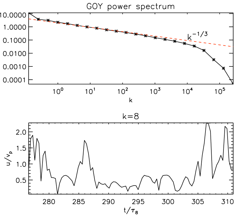
Figure 1.— Velocity spectrum and time series for the GOY model. In the upper panel, we see that the power law of the GOY model is steeper than a Kolmogorov $-1/3$ law, closer to $-0.4$. In the lower panel, we show the velocity time series for the $k=8$ shell, with time normalized to that shell’s own turn-over time.

In Figure 1 we show the velocity spectrum and a sample shell velocity time series. We define a characteristic shell velocity $\overline{u}_{m}$ through the time average of $|u_{m}|$ and $\tau_{m}=1/\overline{u}_{m}k_{m}$, but this is not as perfectly defined as in the fully imposed Kolmogorov case. The GOY model velocity spectrum is also slightly steeper than a Kolmogorov one, a consequence of its intermittency.

2.2. Particles

Figure 2.— Log scale histograms of the total distance $d$ traveled (in box units, box length $2\pi$) for 1000 particles as a function of time for a run with $m_{\text{min}}=2$, $m_{\text{max}}=5$. Overplotted is $ck_{ls}^{-1}(t/\tau_{ls})^{1/2}$ where $c=2/3$.

The motion of inertial particles in a fluid is determined by the friction between the particles and the fluid. The resulting drag force entrains the particles along the fluid motion. Particles with a finite friction time $\tau_{p}$ (subscript $p$ referring to particles) are referred to as “inertial” and their motion deviates from that of the gas as long as the particles are not neutrally buoyant (ie. as long as $\rho_{\text{particle}}\neq\rho_{\text{gas}}$). In this work we assume that $\rho_{\text{particle}}\gg\rho_{\text{gas}}$ which extremely well satisfied for protoplanetary disks. This allows us to neglect pressure forces on the particles. We initialize our particles with a frictional stopping time $\tau_{p}$, so that the equation for a particle’s velocity $\mbox{\boldmath$u$}{}_{p}$ is determined by

$$\frac{\partial\mbox{\boldmath$u$}{}_{p}(t)}{\partial t}=-\frac{\mbox{\boldmath$u$}{}_{p}(t)-\bm{V}(\bm{x}_{p},t)}{\tau_{p}},$$ (9)

where $\bm{V}(\bm{x}_{p},t)$ is the gas velocity at the particle’s position $\bm{x}_{p}$. It is this deviation of the particle velocity from that of the gas that allows particles to collide even in incompressible flows.

When we evolve our particles in the velocity field given by Equation (4), we find a particle velocity dispersion

$$\langle|u_{p}^{2}|\rangle^{1/2}\simeq\frac{v_{m_{\text{min}}}}{\left(1+\tau_{p}/t_{ls}\right)^{1/2}},$$ (10)

that matches the results expected since Völk et al. (1980). Further, in Figure 2 we show log scaled histograms of the total distance $d$ traveled in box length units (box side=$2\pi$, bin size=$0.5$) for a population of $1000$ particles in our base setup (see Section 3). The time axis is scaled to the turnover time of the largest scale turbulence (time between samples $0.2\tau_{ls}$). We overplot $0.67k^{-1}_{ls}(t/\tau_{ls})^{1/2}$, which has the form and approximate scale of a random walk on the length and time scales of the largest scale turbulence. We can see that the particles’ displacements are well fit by the random walk expected to be generated by the largest scale turbulent motion.

In this work we consider only particles with identical stopping time $\tau_{p}$ set to the turnover time of the shell $m_{p}$ with $m_{\text{min}}<m_{p}<m_{\text{max}}$. We will therefore refer to $k_{m_{p}}$ and $v_{m_{p}}$ as $k_{p}$ and $v_{p}$. In the limit of an infinite inertial range, this scale is the only scale, and so most of our values will be non-dimensionalized with respect to it. However, we can investigate the dependence of the collisional velocities on both smaller and larger eddies by turning on and off eddies of differing scales, i.e., by changing $m_{\text{min}}$ and $m_{\text{max}}$.

We are primarily interested in dust collisions in protoplanetary disks, which allows some simplifications. The large size of the Kolmogorov scale turbulence in protoplanetary disks (at a minimum kilometer scale), along with the small size of the dust grains (quite sub-meter for grains embedded well within the inertial range) means that when considering the collisions of protoplanetary dust grains we must treat our dust-grains as point particles, taking limits as the particle separation tends to zero. This is a distinguishing feature compared to atmospheric turbulence, whose Kolmogorov scale might be $1$mm (Shaw, 2003; Xu & Bodenschatz, 2008), comparable to rain drops or particulates. Finally, the actual collision rate of dust grains in protoplanetary disks is expected to be modest due to their dust grain number density: grains will experience multiple friction times between collisions. Accordingly, given our focus on protoplanetary disks we do not treat collisional scattering of the grains.

It is traditional to non-dimensionalize the particles’ stopping time to the Stokes number by scaling it to the turbulent turnover time at the dissipation scale (or occasionally to the time at the driving scale). Unfortunately neither definition fits our setup well, but one can define $St\sim(k_{ss}/k_{p})^{2/3}$ as a conceptual equivalent to scaling $\tau_{p}$ to the dissipation scale since $k_{ss}$ is the smallest scale included in our simulation. Similarly, $St\sim(k_{ls}/k_{p})^{2/3}$ is a conceptual equivalent to scaling $\tau_{p}$ to the turbulent time at the driving scale. However, in Appendix A we explain why we do not consider either approach to be conceptually important as we explicitly hope to achieve large enough inertial ranges that the results are independent of $St$ (either definition). We do define our effective Stokes number according to the first definition above, ${St^{\prime}}\equiv(k_{ss}/k_{p})^{2/3}$, for use when we need to scale diagnostics to the smallest included scale. While it is not a perfect apples-to-apples comparison, this value should be used when comparing with most other work (e.g Bec et al. 2010a; Pan et al. 2011; but not Ormel & Cuzzi 2007, where the other definition is called for).

2.3. Run details

Table 1Runs

Run $m_{\text{min}}$ $m_{p}$ $m_{\text{max}}$ Notes Basic Turbulence (Section 2.1) B-A $0$ $4$ $6$ Smallest $\tau_{p}/\tau_{ls}$ B-B $0$ $3$ $5$ B-LI2 $0$ $3$ $7$ Largest inertial range $k_{7}/k_{0}=128$ B-C $1$ $3$ $5$ B-LI1 $1$ $3$ $7$ Large inertial range $k_{7}/k_{0}=64$ Base $2$ $3$ $5$ Subject of Section 3 B-D $2$ $3$ $6$ B-E $2$ $3$ $7$ B-F $2$ $3$ $8$ Largest ${St^{\prime}}=10$ Quenched Spatial Projection (Section 2.1) Q-A $2$ $3$ $5$ Q-LI $0$ $3$ $7$ Largest inertial range $k_{7}/k_{0}=128$ Varying Phase (Section 2.1) P-A $2$ $3$ $5$ P-LI $0$ $3$ $7$ Largest inertial range $k_{7}/k_{0}=128$ GOY Turbulence (Section 2.1.1) G-A $1$ $3$ $6$ G-B $2$ $3$ $5$ G-C $2$ $3$ $6$ G-LI $0$ $3$ $7$ Largest inertial range $k_{7}/k_{0}=128$

In Table 1 we collect the details of the simulations we perform. The total inertial range is given by $2^{m_{\text{max}}-m_{\text{min}}}$, the effective Stokes number by ${St^{\prime}}=2^{2/3(m_{\text{max}}-m_{p})}$, and the range between the largest scale turbulence and the particles is given by $2^{m_{p}-m_{\text{min}}}$. In all cases the time-step used to advance the particles was $0.1\tau_{ss}$. For runs using the GOY model, the GOY model is advanced for $3\times 10^{7}$ time steps before the introduction of particles, to allow the turbulence to find its statistical steady state. The GOY equations are run with their own time-step of approximately $10^{-4}$ in code units (tweaked to fit an integer number of times within a particle’s time-step); this shorter time-step is for the numerical stability of the algorithm. The particles are initialized with $u=0$ at random positions.

We generate the $\bm{k}_{mn}$ and $\mbox{\boldmath$v$}{}_{mn}$ vectors of Equation (4) by randomly selecting $\bm{k}_{m1}$ from the set of vectors with approximately appropriate length (the error decreases as the target $|\bm{k}|$ increases) that fit in the periodic box. The vector $\mbox{\boldmath$v$}{}_{m1}$ is generated as a random unit vector perpendicular to $\bm{k}_{m1}$. The vector $\bm{k}_{m2}$ is then selected from the set of vectors of appropriate length that fit in the box and lie within $30$ degrees of $\mbox{\boldmath$v$}{}_{m1}$. Next we choose $\mbox{\boldmath$v$}{}_{m2}=\bm{k}_{m1}\times\bm{k}_{m2}/|\bm{k}_{m1}\times\bm{k}_{m2}|$, and repeat the process for $\bm{k}_{m3}$ and $\mbox{\boldmath$v$}{}_{m3}$. If no vector $\bm{k}_{m2}$ or $\bm{k}_{m3}$ can be found that satisfy the constraints, the process is restarted.

3. Analysis: Behavior

We begin by making a full analysis of the run “Base” (Table 1, smallest inertial range) to extract the behavior of the system, both with respect to clustering and collision speeds, and to find a fit formula that can be applied in simulations of particle size evolution. In Section 4 we will study how both increasing the inertial range and changing our turbulence model affects the behavior.

We will obtain our particle clustering and collisional velocity data by analyzing during run time snap-shots taken every full turbulent turnover $\tau_{ls}$ for the largest eddy in the system; these snap-shots include every particle’s position and velocity. The particle positions are mapped onto a coarse grid, and every particle pair within a critical separation (at most $0.2$ of the grid scale) is found. We bin our particle pairs simultaneously linearly in separation $R$, using either $50$ or $100$ bins depending on the run, and linearly in relative velocity $u$. We consider full spheres, so for every $R$ we consider every particle pair with $|\bm{x}_{1}-\bm{x}_{2}|<R$. A bin listed with velocity $u_{\rm{bin}}$ contains particle pairs with relative velocity $u_{\rm{bin}}-\triangle u<u<u_{\rm{bin}}$ where $\triangle u=u_{\rm{max}}/n_{u}$, $u_{\rm{max}}$ is the largest considered particle pair relative velocity and $n_{u}=2000$ is the number of velocity bins. For run Base, $\triangle u=4\times 10^{-4}$ in code units . Particle pairs with relative velocities larger than $u_{\rm{bin}}$ are included in that bin, so it is discarded. We will refer to the total number of pairs in bin $(R,u)$ of snapshot $t$ as $N(R,u,t)$, with dropped $u$ implying summation over all velocity bins and dropped $t$ implying averaging over snapshots.

We took $529$ snap-shots from run Base, but as discussed below, for most of the analysis we drop the first twenty, accordingly, $N(R,u)$ and $N(R)$ are averaged over $509$ snap-shots.

3.1. Clustering

Figure 3.— Particle pairs $N(R,t)$ (unnormalized count) as a function of time for run Base. Top panel: counts for a collisional sphere $Rk_{p}=0.02$. Middle panel: early time blow-up of top panel. Bottom panel: Clustering C(R), with a power-law fit in red/dashed.

In the top two panels of Figure 3 we show $N(R,t)$ as a function of time for a representative maximal separation $R$. We further define the clustering $C(R)$ as the ratio of $N(R)$ to the expected number of particle pairs

$$\overline{N}(R)\equiv\frac{1}{2}n_{p}\times\left(\frac{4\pi R^{3}}{3}\frac{n_{p}}{V}\right),$$ (11)

$$C(R)=N(R)/\overline{N}(R),$$ (12)

assuming a spatially homogenous particle distribution, where $n_{p}$ is the number of particles and $V$ is the volume of the box. A value of $C(R)>1$ implies that particles have been concentrated on length scales $R$, while $C(R)<1$ implies some form of segregation or effective repelling. The clustering $C(R)$ is the same as the $g(St,r)$ of Pan et al. (2011), modulo the differences between ${St^{\prime}}$ and their Stokes number. Their length scale $\eta$ might be understood as our $k^{-1}_{ss}$, although their turbulence at that scale is explicitly affected by dissipation, and so the energy is no longer following a turbulent cascade.

The particles are initialized with zero velocity and random initial position, and in the top and middle panels of Figure 3 we see that the number of particle pairs takes more than ten largest-scale turn-overs to stabilize (more than $16$ particle friction times), and still shows significant fluctuations. This long stabilization time is an important observation which helps explain results later in this paper: there is significant structure in the particle distribution that takes time to develop, and studies of particle collisions need to consider a significant time interval. Unfortunately, including a history of ten full largest-scale turnovers is beyond current or foreseeable analytical analyses. Clearly particle positions are quite correlated with one another. In what analysis that follows, we discard the first twenty snap-shots to allow the system to stabilize.

In the bottom panel of Figure 3 we show $C(R)$ which shows a clear power-law dependence on the maximal separation $R$. We will denote by $\mu$ the power-law $C(R)\propto R^{-\mu}$, and by $R_{1}$ the intercept where the power-law fit gives $1$.

3.2. Average collision energy

Figure 4.— Average collisional speed between particles as a function of maximal separation for run Base. Note the small scale of the horizontal axis.

A first calculation of the rms-collisional velocity is shown in Figure 4 where we plot

$$\overline{u}_{c}(R)\equiv\left(\frac{\Sigma_{u}N(R,u)u^{3}}{\Sigma_{u}N(R,u)u}\right)^{1/2}.$$ (13)

The factor of $u$ in the denominator is needed to convert from particle pairs to particle collision rates: because we are taking well-separated snapshots we need to weight high velocity pairs more heavily. A naive expectation would be that the collisional velocity decreases with decreasing $R$, reaching a finite plateau at small separation, such as seen in Bec et al. (2010b). This finite plateau is made possible by the compressible nature of the particle “fluid”, even if the turbulent gas itself is incompressible. In Figure 4 we are already in this plateau, but see an increasing collisional velocity with decreasing $R$ (except for the smallest $R$, where our pair-counts are too low for reliability).

This perhaps surprising result does not flow from poor statistics, but rather is a robust and understandable consequence of the clustering seen in the bottom panel of Figure 3. The clustering seen there increases strongly with decreasing $R$, implying a relatively numerous population of highly correlated particles. As $R$ decreases, the relative particle-particle velocities in this highly correlated population must decrease for the pairs to stay within the cluster radius: the smaller $R$, the lower the relative velocities of the correlated population must be. We might guess that the characteristic relative velocity of this population is linear in $R$, giving a constant crossing-time. Since the power-law fit in Figure 3 is weaker than $R^{-1}$, the contribution of this population to the denominator of Equation (13) decreases with decreasing $R$. The velocity plateau at larger separations implies that the highly correlated population has already ceased to contribute meaningfully to the numerator due to the extra factor of $u^{2}$. Even at the largest separations $R$ we consider in Figure 4, the relative velocity of the highly correlated population is low enough that this population contributes only negligibly to the total collisional power. In effect, the highly correlated population is diluting the collisional energy when an average is taken, and this dilution is decreased by considering smaller $R$.

Since we are considering point particles, we must consider the limit $R\rightarrow 0$, and in that limit, the highly correlated population appears to play a dominant role in the pair counts (because $\mu>0$), but contributes no collisions (since $\mu<1$). We accordingly define this collisionless population as “cold” (low relative velocities). Unfortunately, numerical resource constraints prevent us from considering values of $R$ small enough that the cold population has ceased to contribute meaningfully to straightforward calculations of the collision rate (the denominator of Equation 13). Note that this is different from the expectations of, for example, Pan et al. (2011), where turbulent clustering was hypothesized to lead to more common collisions by increase the number of nearby potential collisional partners. As we will see, however, there is a significant chance that some level of clustering will persist, albeit not one that scales inversely with $R$.

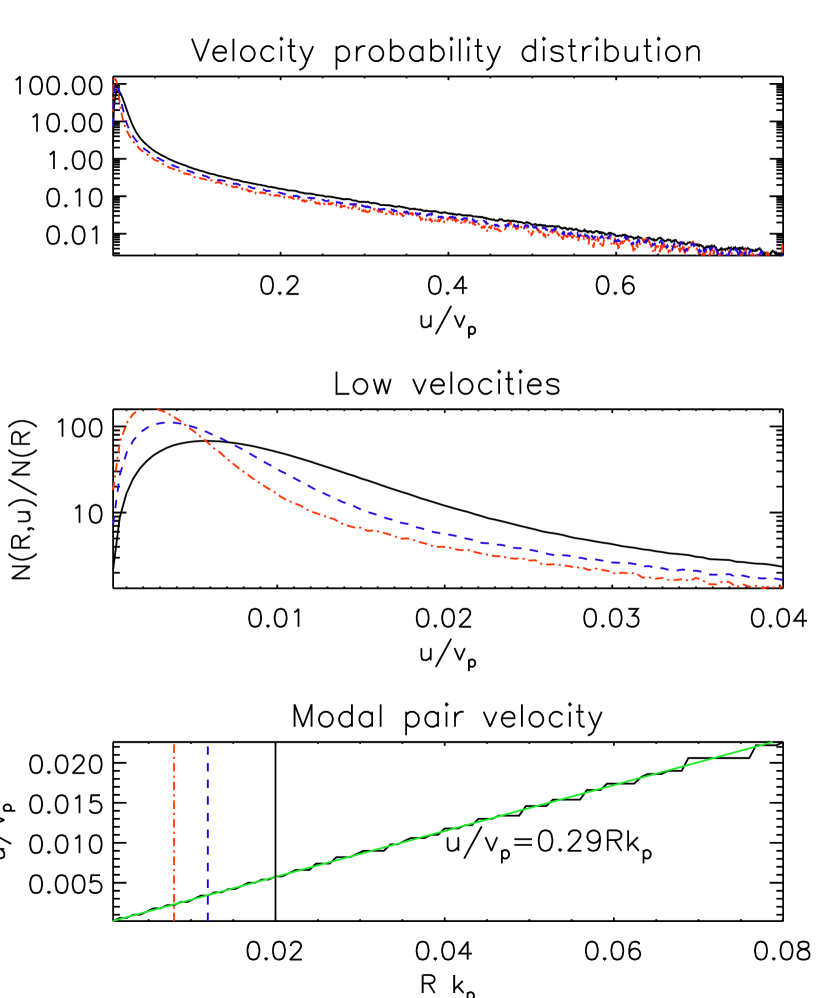
Figure 5.— Top and middle panels: particle relative velocity probability distributions for three different $R$ in run Base. Black: $Rk_{p}=0.02$, blue/dashed: $Rk_{p}=0.012$, red/dash-dotted: $Rk_{p}=0.008$; see also the top panels of Figure 6. Bottom panel: the velocity of the peak as a function of R along with a linear fit in green. The vertical lines show the position of the three cases of the top two panels.

The implications of this interpretation of Figure 4 are seen in Figure 5, where

$$N^{\prime}(R,u)\equiv N(R,u)/\triangle u$$ (14)

is the density of pairs within separation $R$ in velocity space (to convert between binned data and a smooth distribution). The probability distribution is seen to be strongly affected by a low velocity peak which moves to smaller velocity linearly with $R$, to a limit of $0$ as $R\rightarrow 0$ (compare with Carballido et al. 2010, Figure 5, which is lin-log instead of log-lin). We define

$$\omega\equiv u_{cold}/R,$$ (15)

as the measure of the dependence of the velocity of the cold population on separation, where $u_{cold}$ is the modal pair velocity.

This collisionless behavior of the cold population does not mean that we expect no collisions. As can be seen in the top panel of Figure 5, $N(R,u)$ has a significant high velocity tail, which can contribute “real” collisions. A process to excise the cold, collisionless population and fit the remainder is discussed below.

3.3. Fitting

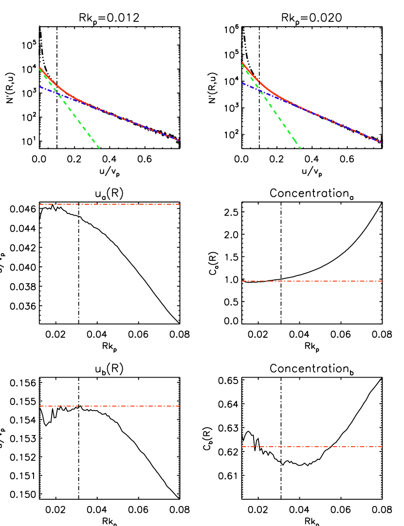
Figure 6.— Top panels: fits using Equation (16) for run Base. Black/dash-triple-dotted: data, red/solid: total fit, green/dashed: fit component $a$, blue/dash-dotted: fit component $b$. Only the region to the right of the vertical line $u=u_{c}$ is fitted. Left panels: $u_{a}$ and $u_{b}$, along with their maxima in the non-contaminated region to the left of the vertical line $R=R_{c}$. Right panes: $C_{a}$ and $C_{b}$, along with their means in the non-contaminated region to the left of the vertical line $R=R_{c}$.

We have failed to successfully fit the cold, clustered population with a tractable distribution such as a Weibull distribution; however the tail of the pair-probability distribution in velocity space is well fit by a simple exponential, and at more modest velocities the addition of a second exponential improves matters. Accordingly, we fit the particle-pair probability distribution by

$$N^{\prime}(R,u>u_{c})/\overline{N}(R)=\frac{C_{a}}{u_{a}}e^{-u/u_{a}}+\frac{C_{b}}{u_{b}}e^{-u/u_{b}},$$ (16)

$$u_{c}=0.1v_{p}$$ (17)

but only for $u>u_{c}$, where $u_{c}$ is a cut-off designed to exclude the cold population. The fit formula Equation (16) identifies two separate populations $a$ and $b$ with $u_{a}<u_{b}$. While we do not have an analytical theory for the form of Equation (16), the quality of the high velocity component $b$ can be seen from the overlap between the blue/dash-dotted curves (the higher velocity component) and the black/dash-triple-dotted curve (data) in Figure 6. The fit for component $a$ to be less well constrained, but it gives a noticeable different at lower relative velocities, seen in the difference between the blue/dash-dotted curve (only component $b$), and the red/solid curve (both components, overlays the data outside of $u_{c}$). We refer to component $a$, handling the lower relative velocities, as the “warm” population, and the fit component $b$, handling the higher relative velocities, as the “hot” tail.

The parameters $C_{a}$ and $C_{b}$ then set the clustering of the effective densities of the warm and hot populations compared to the total population were it homogeneously distributed (see Equation 12). Finally, we define a contamination radius

$$R_{c}=0.2u_{a0}/\omega$$ (18)

outside of which the cold population is considered to contaminate the results, i.e., where $u_{cold}$ from Equation (15) is comparable to $u_{a}$. The factor of $0.2$ is chosen ad-hoc, but is inspired by the middle panels of Figure 6; $u_{a0}$ is an approximate value for $u_{a}$. The fit parameters in Equation (16) are functions of $R$, but as seen in Figure 6 meaningful limits $R\rightarrow 0$ can be taken. The reported values of $C_{a}$, $C_{b}$, are averaged over the non-contaminated region, while the reported values of $u_{a}$, and $u_{b}$ are the maximum value inside the non-contaminated region.

3.4. Weights and errors

Our reported fit coefficients $u_{a},u_{b},C_{a}$ and $C_{b}$ depend on the weighting scheme, the fitting region, and $u_{a0}$. We weight with

$$W=[1/N(R,u)]\times\left[1+\frac{2(u-0.7u_{\rm{M}})(u-u_{c})}{(0.7u_{\rm{M}}-u_{c})^{2}}\right],$$ (19)

where $u_{\rm{M}}$ is an upper velocity cut-off imposed when the number of pairs/bin approaches unity. This weighting scheme weights the low velocity (warm) and high velocity (hot) regions more highly, allowing the two populations to be distinguished by the fitting algorithm. The values of $N^{\prime}(R,u)$ in Figure 6 have a minimum $\sim 10$. As we are averaging over $509$ snap-shots, with $\triangle u=4\times 10^{-4}$, that corresponds to $\sim 2$ pairs per bin which is a consequence of our large number of velocity bins, $2000$. To avoid zeroes we have smoothed over $20$ bins in velocity space. The effect of sampling noise can be gauged from the middle and bottom panels of Figure 6 as the limit $R\rightarrow 0$ is taken with a corresponding reduction in pair count, especially at high relative velocity. As the fitting procedure is somewhat qualitative, we will be more interested in the scale of the results, and any trends with varying $m_{\text{min}}$ and $m_{\text{max}}$, rather than in precision. As we will discuss in Section 5, our collisional velocities are factors of order five slower than previous work, well outside any systematic or statistical errors.

4. Analysis: Inertial Range, Turbulence Models

4.1. Clustering

Table 2Clustering diagnostics

Run $m_{\text{min}}$ $m_{p}$ $m_{\text{max}}$ ${St^{\prime}}$ $\mu$ $R_{1}k_{p}$ $\omega\tau_{p}$ $R_{c}k_{p}$ B-A $0$ $4$ $6$ $2.5$ $0.65$ $1.6$ $0.29$ $0.04$ B-B $0$ $3$ $5$ $2.5$ $0.57$ $1.9$ $0.27$ $0.04$ B-LI2 $0$ $3$ $7$ $6.3$ $0.39$ $1.6$ $0.55$ $0.02$ B-C $1$ $3$ $5$ $2.5$ $0.55$ $1.7$ $0.23$ $0.04$ B-LI1 $1$ $3$ $7$ $6.3$ $0.38$ $1.8$ $0.55$ $0.02$ Base $2$ $3$ $5$ $2.5$ $0.49$ $1.6$ $0.29$ $0.03$ B-D $2$ $3$ $6$ $4$ $0.45$ $1.5$ $0.39$ $0.02$ B-E $2$ $3$ $7$ $6.3$ $0.38$ $1.2$ $0.52$ $0.02$ B-F $2$ $3$ $8$ $10$ $0.38$ $1.2$ $0.76$ $0.02$ Q-A $2$ $3$ $5$ $2.5$ $0.34$ $5.0$ $0.51$ $0.03$ Q-LI $0$ $3$ $7$ $6.3$ $0.44$ $13$ $0.50$ $0.03$ P-A $2$ $3$ $5$ $2.5$ $0.81$ $0.8$ $0.21$ $0.03$ P-LI $0$ $3$ $7$ $6.3$ $0.40$ $2.2$ $0.39$ $0.03$ G-A $1$ $3$ $6$ $3.7$ $0.36$ $1.9$ $0.14$ $0.02$ G-B $2$ $3$ $5$ $2.4$ $0.40$ $2.0$ $0.16$ $0.03$ G-C $2$ $3$ $6$ $3.7$ $0.33$ $2.7$ $0.14$ $0.03$ G-LI $0$ $3$ $7$ $5.9$ $0.38$ $1.8$ $0.20$ $0.02$

In Table 2 we present the basic clustering data for our turbulence models, across an array of inertial ranges and our turbulence models. Parameters $m_{\text{min}},m_{p},m_{\text{max}}$ and ${St^{\prime}}$ define the included inertial range, as well as an effective Stokes number. The diagnostics $\mu$ and $R_{1}$ are the power-law and intercept of the power-law fit to $C(R)$ (Section 3.1) while $\omega$ defines the relative velocities of the cold population (Equation 15) and $R_{c}$ defines the contamination radius outside of which the collisionless cold population becomes indistinguishable from the collisional warm and hot populations.

There appears to be a modest decrease of the clustering parameter $\mu$ with the number of shells with turnover times shorter than the particle drag time $\tau_{p}$, as measured by ${St^{\prime}}$. However, it also appears to increase with the number of shells included with turnover times longer than $\tau_{p}$. Comparing runs B-E, B-F, B-LI1, and B-LI2, we feel that we have reached a large enough inertial range to estimate that particles well embedded in turbulence will experience clustering with $\mu\sim 0.4$. This result matches the behavior with other turbulence models, although run P-A is a clear outlier.

Another interesting column is $\omega\tau_{p}$. This value scales slightly slower than ${St^{\prime}}$, and $\omega^{-1}$ is the crossing time of a cold cluster. Accordingly, the result is that the crossing time of the cold cluster scales slightly slower than the turnover time of the smallest included eddy, supporting the extension of the hypothesis that the cold velocity is linear with separation (Eq. 15) to an infinite cascade without meaningful smallest scale. This is further born out by the results for the other turbulence models, particularly the GOY model, which see weak or no dependence of $\omega$ on ${St^{\prime}}$.

A problematic column is $R_{c}k_{p}$. This imposes the minimal spatial resolution required to make a meaningful analysis of dust collisions by discarding the cold population. In a $2\pi^{3}$ box with $k_{p}=8$ (assuming an energy carrying scale of $k=4$), a grid scale with $\triangle x=R_{c}$ requires a resolution on the order of $1700^{3}$ even for our smallest inertial range. This smallest range is within reach, albeit barely (Bec et al., 2010a, b).

4.2. Collisions

Table 3Collisional diagnostics

Run $m_{\text{min}}$ $m_{p}$ $m_{\text{max}}$ ${St^{\prime}}$ $C_{a}$ $C_{b}$ $u_{a}/v_{p}$ $u_{b}/v_{p}$ B-A $0$ $4$ $6$ $2.5$ $1.1$ $0.46$ $0.070$ $0.21$ B-B $0$ $3$ $5$ $2.5$ $1.2$ $0.57$ $0.056$ $0.20$ B-LI2 $0$ $3$ $7$ $6.3$ $1.7$ $0.92$ $0.069$ $0.19$ B-C $1$ $3$ $5$ $2.5$ $0.9$ $0.42$ $0.054$ $0.18$ B-LI1 $1$ $3$ $7$ $6.3$ $1.5$ $0.89$ $0.069$ $0.17$ Base $2$ $3$ $5$ $2.5$ $1.0$ $0.62$ $0.046$ $0.15$ B-D $2$ $3$ $6$ $4$ $1.1$ $0.83$ $0.054$ $0.17$ B-E $2$ $3$ $7$ $6.3$ $1.1$ $1.0$ $0.057$ $0.16$ B-F $2$ $3$ $8$ $10$ $1.2$ $1.1$ $0.064$ $0.17$ Q-A $2$ $3$ $5$ $2.5$ $1.4$ $1.4$ $0.077$ $0.48$ Q-LI $0$ $3$ $7$ $6.3$ $2.8$ $2.0$ $0.13$ $0.71$ P-A $2$ $3$ $5$ $2.5$ $0.5$ $0.25$ $0.036$ $0.098$ P-LI $0$ $3$ $7$ $6.3$ $1.5$ $0.37$ $0.050$ $0.134$ G-A $1$ $3$ $6$ $3.7$ $0.7$ $0.31$ $0.070$ $0.22$ G-B $2$ $3$ $5$ $2.4$ $0.7$ $0.43$ $0.077$ $0.32$ G-C $2$ $3$ $6$ $3.7$ $0.7$ $0.31$ $0.068$ $0.20$ G-LI $0$ $3$ $7$ $5.9$ $0.8$ $0.37$ $0.076$ $0.24$

In Table 3 we collect fit data for our simulations, which should only be used for intermediate and higher relative velocities ($u>u_{c}=0.1v_{p}$, see Equations 16 and 17). Parameters $m_{\text{min}},m_{p},m_{\text{max}}$ and ${St^{\prime}}$ define the included inertial range, as well as an effective Stokes number, while the diagnostics $C_{a},C_{b},u_{a}$ and $u_{b}$ are the coefficients in our fit formula Equation (16). Coefficients $C_{a}$ and $C_{b}$ describe the effective target number density seen by the warm and hot populations respectively, and coefficients $u_{a}$ and $u_{b}$ represent the velocity scale of the two populations.

The $C_{a}$ and $C_{b}$ columns indicate that the warm and hot populations, in the velocity regime where the fit applies, have individual effective densities comparable to the density that the total dust population would have were it evenly distributed. This does not strictly imply that there is clustering of the collisional population, because many of the collisions are likely at low, unfitted velocities. The results for $C_{a}$ and $v_{a}$ are the least useful, as they are most sensitive to the cold population, and $u_{a}<u_{c}$. The results for $u_{b}$ are nicely only weakly sensitive to the set of included shells, while $C_{b}$ appears to require a significant ${St^{\prime}}\simeq 10$ to reach a limiting value.

Most of our diagnostics, such as $u_{a},u_{b},C_{a}$ and $R_{1}$ appear to be relatively insensitive to the set of included shells, i.e., $(m_{\text{min}}-m_{\text{max}})$ and ${St^{\prime}}$. It should nonetheless be noted that since the diagnostic $u_{b}$ is crucial to the high velocity collisions which might result in fragmentation, its weak sensitivity to $m_{\text{min}}$ is still important. Achieving converged values for $C_{b}$, an important diagnostic, certainly requires ${St^{\prime}}\gtrsim 6$, while the behavior of $C_{a}$ in the limit of both larger and smaller eddies is not yet clear (bottom two lines of Table 3). Accordingly, ranges of $k_{p}/k_{ls}=8$ and $k_{ss}/k_{p}=16$ appear to be reasonable minimums. Unfortunately, it appears that extreme resolution is required not merely to include an adequate inertial range, but also to capture the details of particle clustering.

Comparing the results across different turbulence models, a first observation is that they are well fit by Equation (16), as seen in Figure 7, albeit with differing parameters. The fully quenched model (runs Q-A and Q-LI) produces both significantly more concentrated collisions (the $C$ coefficients), and significantly higher collisional velocities. This is not particularly surprising as there is nothing to destroy long time correlations. Putting the time variation of the spatial projection into the phase (runs P-A and P-LI) however results in a significant drop in the collisional velocities. Finally, the GOY model appears to fit with very similar velocity parameters of our base model although the clustering is weaker. This is somewhat surprising as the turbulence is spiky, which might be expected to result in a stronger high velocity tail. On the other hand, it inherently includes phase variation. A further unexpected detail of the GOY model is that the smallest range of included shells ($m_{\text{min}}=2$, $m_{\text{max}}=5$) showed the strongest high velocity tail ($u_{b}=0.32v_{p}$). This may be due to the fact that the GOY scheme has an intermittent energy cascade, and the generation of sub-vortices from larger vortices (a consequence of localized energy spikes in $k$-space, through the coupling terms of Equation 2.1.1), if appropriately followed by including an adequate inertial range to track the sub-vortices, will decrease particle correlations.

Finally, we suggest that Equation (16) be used with parameters of the order of $C_{a}\sim 1.5$, $C_{b}\sim 1$, $u_{a}\simeq 0.07v_{p}$ and $u_{b}\simeq 0.2v_{p}$, applying only when relative velocities exceed the cut-off velocity $u_{c}=0.1v_{p}$, i.e.,

$$\frac{N(R,u>0.1v_{p})}{\overline{N}(R)}=\frac{21}{v_{p}}e^{-14u/v_{p}}+\frac{5}{v_{p}}e^{-5u/v_{p}}.\\$$ (20)

If one prefers the GOY model, the concentration parameters should be changed to $C_{a}\sim 0.8$ and $C_{b}\sim 0.4$.

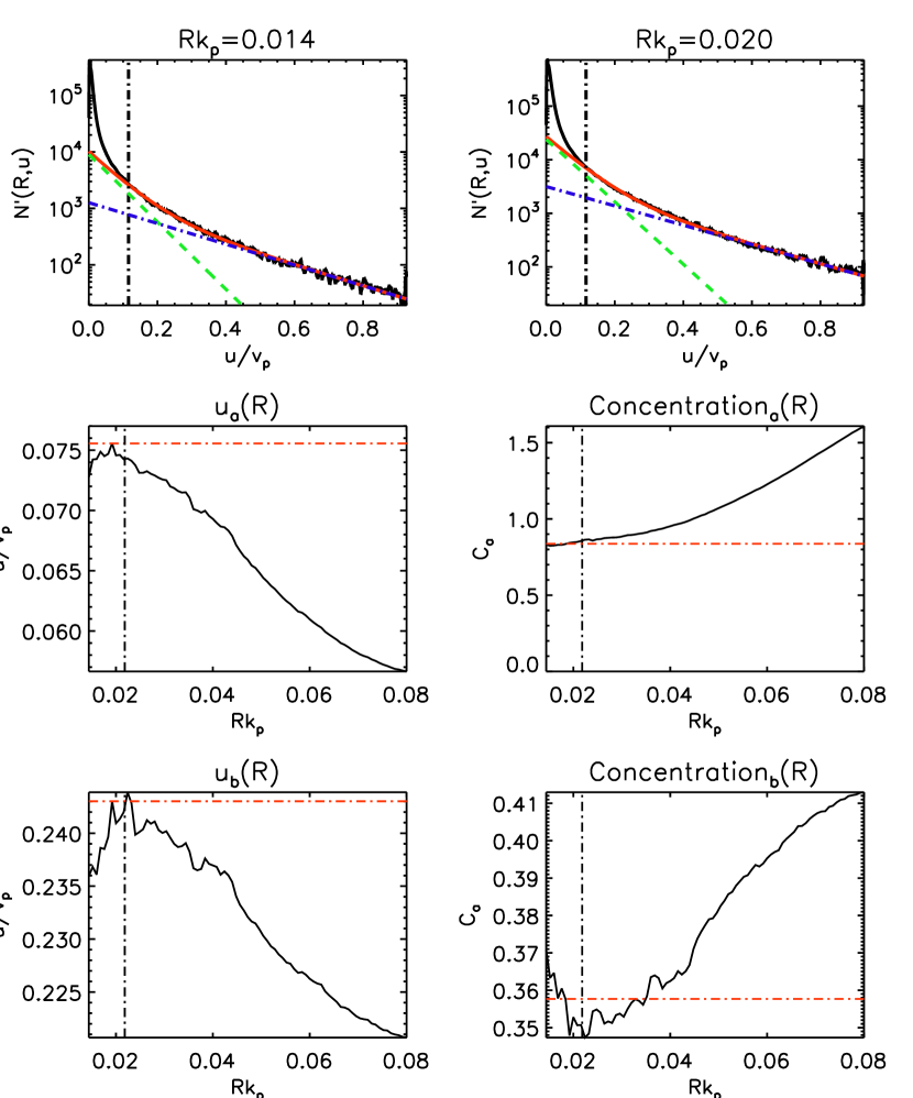
Figure 7.— As in Figure 6, but here we show run G-LI. Averaged over $112$ snap-shots, with $\triangle u=4.64\times 10^{-4}$ in code units.

5. Comparison with previous work

5.1. Clustering

Turbulent clustering has been a topic of interest in the protoplanetary community, and has been invoked, for example, in the creation of chondritic meteorites (Cuzzi et al., 2001). Our clustering diagnostics follow those of Pan et al. (2011), rather than those of Fessler et al. (1994); Hogan & Cuzzi (2001). The previous work found evidence for strong clustering for particles with modest $St$, i.e., particles reasonably well coupled to turbulence at the dissipation scale. The clustering of Pan et al. (2011) was observed to decrease as their Stokes number became different from $1$. Our results fit in magnitude with those of Pan et al. (2011), which scale up to $\mu\gtrsim 0.6$ (see their Figure 6). However, our clustering is significantly stronger at high $St$ or ${St^{\prime}}$. Given the differences in the fluid flows used (synthetic turbulence in our case, forced turbulence in Pan et al. 2011), the similarities in behavior and scale of the exponent are encouraging. However, it isn’t clear from the $\mu$ column in Table 2. that clustering will cease for large ${St^{\prime}}$, as previously seen. It should be noted that previous simulations had limited inertial ranges, so their high St particles are not fully embedded in the turbulence (see Appendix A).

There is reason to expect that clustering will be more effective for particles with $\mbox{\rm St}=1$ (Cuzzi et al., 2001; Hogan & Cuzzi, 2001). However, we can imagine evolving a system of two species of particles with $\mbox{\rm St}_{1}=1$ and $\mbox{\rm St}_{2}\ll 1$. Once a statistical steady-state is achieved, with the $\mbox{\rm St}_{1}$ particles more strongly clustered than the $\mbox{\rm St}_{2}$ particles, we decrease the fluid viscosity significantly so that in the new flow, $\mbox{\rm St}_{1}\gg 1$ and $\mbox{\rm St}_{2}=1$ because the new dissipative scale is smaller. At that point, even if the $\mbox{\rm St}_{2}$ particles are more strongly clustered than the $\mbox{\rm St}_{1}$ particles, it isn’t clear why the $\mbox{\rm St}_{1}$ particles would be less clustered than originally. Runs Base through B-F in Table 2 match this thought experiment, and do show a drop of $\mu$ from $0.49$ to $0.38$ which appears to be a minimal value. This weak decrease in $\mu$ may result from particle clusters being disrupted by the additional, smaller-scale, eddies.

Pan et al. (2011) hypothesized that clustering, especially if it exists for $St>1$, might greatly increase the collision rates between particles by generating regions of enhanced particle number density. Our results allow us to contradict the straightforward version of that hypothesis: the clustering exists, but the particle clusters are non-collisional. However, once particle number densities get high enough that the dust fluid density is comparable to the gas density, the dust drag has a significant back-reaction on the gas. An example is the streaming instability. In protoplanetary disks, gas orbits in a sub-Keplerian fashion because of the outwards pointing pressure force. As a result, particles, which would naturally orbit in a Keplerian fashion, feel a headwind. Similarly to drafting on highways or in bicycle races, clumps of particles can then form which are dense enough to back-react on the gas (Cuzzi et al., 2001; Youdin & Goodman, 2005; Johansen et al., 2007; Lewellen et al., 2008).

5.2. Collisions

Much of astrophysical turbulent dust collision work follows the approach of Völk et al. (1980); Markiewicz et al. (1991); Cuzzi & Hogan (2003); see Ormel & Cuzzi (2007) for a recent. This approach defines two classes of eddies, Class I large-scale eddies and Class II small-scale eddies. The former have large velocities and time scales, and so can transport dust grains significant distances: they dominate the turbulent diffusion of dust throughout a disk or atmosphere. On the other hand, they change slowly enough in both space (compared with dust stopping lengths) and time (compared with $\tau_{p}$) that nearby dust grains, which could collide, see nearly identical gas motion. As a result, Class I eddies can affect the collisional behavior of dust grains only slightly. Class II eddies on the other hand vary rapidly compared to both the frictional stopping time of the dust grains and their stopping length. Accordingly, these eddies can affect even nearby dust grains differently, driving collisions. However, their short time and length-scales mean that they provide only weak large-scale transport.

Dropping the contribution of Class I eddies for collisions between identical dust grains, Ormel & Cuzzi (2007) find an rms collisional velocity of

$$u^{2}_{\text{Ormel}}=2v_{p}^{2}.$$ (21)

While this result is frequently quoted in terms of the Stokes number defined as $St=\tau_{p}\Omega_{K}$, the above version is more general (see Appendix A). An important assumption is that the relative motion of particles approaches a finite limiting value as their separation goes to zero, which is possible for inertial particles ($\tau_{p}\neq 0$) whose motion must deviate from that of the gas. Such behavior is seen in the direct numerical simulations of Bec et al. (2010b) and we believe we understand the deviation from that assumption seen in our Figure 4. This analytical approach cannot however handle very long time-correlations between dust grains.

The result in Equation (21) is different from our Equation 16 in two ways. First, it is a single number, which does not suffice to describe our results, with their two velocity scales of the warm and hot populations. Our results also have merely exponentially falling probability tails with $u$, a much broader distribution than, for example, a Maxwellian distribution. They should therefore be treated as a probability distribution. Second, if one nevertheless uses Equation (13) to extract a single rms-averaged collisional velocity, we find

$$u_{\text{our}}=\left[\frac{6\left(C_{a}u_{a}^{2}+C_{b}u_{b}^{2}\right)}{C_{a}+C_{b}}\right]^{1/2}\simeq u_{\text{Ormel}}/4,$$ (22)

using the suggested parameters of Section 4.2, a significant decrease in the characteristic collisional velocities and a much larger decrease in the turbulent collisional energies. We attribute this difference in predicted collisional velocities to the high level of correlation we have identified, which not only creates the “cold” population, but appears to slow all the collisions.

One can also compare Figure 4 and the bottom panel of Figure 5 with Figure 4 of Carballido et al. (2010), which is further limited by the sub-gridscale gas velocity interpolation. Clearly, very high spatial resolution is required to extract actual collisional velocities from numerical simulations, at least for particles with identical stopping times. Our method provides large inertial ranges and high resolutions, whose necessity can be seen in their Figure 3, where the analytical result based on a full inertial range, the analytical result based on the actual inertial range and the numerical result all disagree. The resolution to begin to see the multiple populations we have identified in direct numerical simulations of the full Navier-Stokes equation may be becoming available (for example the $2048^{3}$ simulation of Bec et al. 2010a, b which is just adequate to include the inertial range assumed in run Base while resolving $R_{c}$). However the analysis has not been done in the same terms so it is not clear whether they would see the effects we predict, or, if not, it would be because they contradict our results, or do not have adequate resolution.

6. Discussion and Conclusions

Figure 8.— Ad hoc fits for $u<u_{c}$. Left column: extending Equation (20) to $u=0$, Right column: extending the constant value at $u=u_{c}$ to $u=0$. Top panels: pair density, i.e., Equation (20). Middle panels: solid: cumulative totals of the top panels; dashed: $u_{c}$ its intercepts by the data. The right axis is self-normalized. Bottom panels: solid: self-normalized cumulative totals of the collision rate i.e., the first velocity moment of Equation (20); dashed: $u_{c}$ its intercepts.

We arrive at a picture of turbulence-induced particle concentration and collisions which creates spatially small (with respect to turbulent scales), highly correlated “cold” clusters of particles. While these clusters are themselves non-collisional, they periodically pass through each other, resulting in bursts of collisions. These clusters are channeled through the high-strain boundaries between turbulent eddies, and even separate clusters are strongly correlated. This correlation causes the turbulent collision speeds we find to be significantly slower than those predicted by analytical approaches, that cannot treat the long time-scale correlations. This picture of particle-particle collisions occurring when clusters of particles pass through each other is supported by the long stabilization time seen in Figure 3, where it takes many turbulent turnover times to reach a statistical steady state, implying non-trivial dust spatial structures.

Our results apply most strongly for particles deeply embedded in a turbulent cascade. Our approach does not have the ability to handle the details of the forcing scale or the dissipation scale of the turbulence, both of which could have different behavior such as the bottleneck effect at the dissipation scale (Dobler et al., 2003). Nevertheless, the qualitative similarity between our low inertial range runs (Basic, Q-A, P-A, G-A) with the large inertial range runs (B-LI2, Q-LI, P-LI, G-LI) suggests that this will only pose a difficulty if the statistics of the turbulence are indeed quite different at those two scales. A second difficulty is that our synthetic turbulence model cannot handle the dust’s back-reaction on the gas, which can be significant if there is strong clustering. An implicit assumption of our work therefore is that the dust spatial density is less than that of the gas.

We find that Equation (16) is a workable fit for the number of turbulence-induced particles pairs as a function of collisional velocity. This form has some interesting implications. A simple one is that it is broad: unlike the case of, for example, a Maxwellian distribution, enough of collisional velocity space is populated that many collisional outcomes will occur in relevant quantities. Less obviously, we note that in the “high” velocity parameter regime, we can fit the collisional probability distribution through the autocorrelation of exponential decays:

$$C_{b}ue^{-\frac{u}{u_{b}}}=\int_{0}^{u}\left[\sqrt{C_{b}}e^{-\frac{u^{\prime}}{u_{b}}}\right]\left[\sqrt{C_{b}}e^{-\frac{u-u^{\prime}}{u_{b}}}\right]du^{\prime}.$$ (23)

This implies that (faster) collisions are generated by particles each contributing a velocity with respect to the collisional center (which is a feature of the fluid flow rather than the center of mass of the particle pair) with an exponentially falling probability. Note that this is not the difference between the particle velocity and that of the gas, which is, naturally, correlated between the two particles. Why the individual particle probability distribution is an exponential decay, and why the autocorrelation occurs in collision-space ($P(u)\propto ue^{-u/u_{0}}$) rather than in the particle pair space ($P(u)\propto e^{-u/u_{0}}$) is unclear.

Our formula is limited in its applicability to $u>u_{c}$, and as $R$ tends to $0$, neglects almost all the particle pairs since they are part of the cold population (because $\mu>0$, see the height of the peak in the middle panel of Figure 5, which increases as $R$ decreases). This does not appear to pose unsurpassable difficulties: in Figure 8 we show two alternate ad-hoc extensions for Equation (20) into the low $u$-regime. From the bottom panels we can see that it is unlikely that errors in the collision rate based on the extension chosen will be more than $25\%$ of the total: low relative velocity dust grains, even if numerous, contribute few collisions due to their slow speeds. Errors in energy, the square-root of the 3rd velocity moment, will be significantly less yet, as long as there is not a hidden, highly clustered but still collisional population that we have not been able to detect so far.

Another intriguing result is the low scale of $u_{b}\simeq 0.2v_{p}$. This collisional velocity scale is significantly below the predicted rms collisional velocity $u_{\text{col}}=2^{1/2}v_{p}$ of Ormel & Cuzzi (2007). This might be explained by the vertical axes of the middle plots of Figure 8: the limiting value on the left axes gives the effective concentration i.e., the number of pairs in the warm and hot populations, divided by $\overline{N}(R)$. While the difficulties fitting the cold population make the result uncertain, it appears that clustering occurs in the collisional population: particles see more warm and hot collisional partners than would be expected if all dust grains were homogeneously distributed in space. This clustering is different from that of the cold population in that the clustering is independent of $R$ for small separations (i.e., the effective $\mu=0$; an equivalent plot to the bottom panel of Figure 3 would be flat). For any clustering to occur, the colliding particles in the warm and hot populations must still be significantly correlated with one another, an aspect which the work of Ormel & Cuzzi (2007) could not fully capture.

In conclusion, we see turbulence-induced dust collisions at significantly (a factor of 3-5) slower velocities than predicted by existing analytical theory. If we consider an approximate $\alpha$-disk Minimum Mass Solar Nebula with a sound speed of $c_{s}=10^{5}\,$cm/s (temperature $T\simeq 300\,$K) at $1\,$AU, $\alpha=10^{-3}$ and centimeter-scale grains with a stopping time $\tau_{p}\Omega_{K}=0.01$ and mass $m\sim 1\,$ g, the turbulent velocity at the largest scale is $v_{t}=3\times 10^{3}\,$cm/s (Shakura & Sunyaev, 1973; Hayashi, 1981). Under these conditions, the predicted collisional velocity of Ormel & Cuzzi (2007) is $u=5\times 10^{2}\,$ cm/s, well into the destructive collision regime of Güttler et al. (2010), Figure 11. A five-fold reduction in the collision speed would however lead to bouncing. While this result implies frequent destructive collisions, we also predict large numbers of lower velocity collisions, which could lead to sticking. This would ease the difficulties in planetesimal formation associated with bouncing and fragmentation (Zsom et al., 2010). The velocities we expect will still lead to significant fragmentation, but the inclusion of a slower collisional velocity probability distribution allows for the consideration of “lucky” particles that are in unusually low velocity collisions to grow large enough that they can survive. While the slower collisional velocities reduces collision rates, we also see a limited enhancement of the effective dust number density through clustering, which mitigates this collision rate reduction.

Finally, the hot population collisional tail falls off only exponentially with velocity, rather than something closer to a Maxwellian distribution. This emphasizes the importance of using a collisional velocity probability distribution instead of a single characteristic collisional velocity. For example, high velocity outlying events are expected to occur at non-negligible rates, and could contribute to a fragmentation cascade and dust reprocessing. This would occur even if the reduction in collisional velocities results in few enough destructive collisions that the fragmentation barrier to dust growth is lifted.

Our results are well suited to inclusion in a model of collisional dust grain agglomeration in protoplanetary disks such as that of Zsom et al. (2010). The formula given by Equation (16) is simple enough for inclusion, while allowing a velocity probability distribution. This enables the full use of experimental results about the critical velocities at which colliding particles stick, bounce or fragment.

Appendix A Stokes numbers

Studies of turbulent particle transport generally use the Stokes number $St\equiv\tau_{p}/\tau_{\eta}$ to non-dimensionalize the stopping time, where $\tau_{\eta}$ is the turbulent time scale associated with the viscous dissipation scale. Astrophysical studies of protoplanetary disks however often use $St\equiv\tau_{p}\Omega_{K}$, where $\Omega_{K}$ is the Keplerian rotation rate, since it is better constrained than $\tau_{\eta}$ and is believed to be a good estimate for the time scale associated with the largest scale turbulence. As such, the particle stopping time is often scaled to two completely different time scales, the largest and the smallest associated with the turbulence. Neither formulation is however clearly appropriate for studies of particle-particle relative motion and clustering.

Stating that the relevant quantity is $St=\tau_{p}/\tau_{\eta}$ implies that either the details of the dissipation process proper, or the lack of fluid energy at scales $k>k_{\eta}$ plays a crucial role in the particle response to the turbulence. For a particle with $St\lesssim 1$, such effects are expected, as particles couple most strongly with eddies with turnover times $t\sim\tau_{p}$ and the dissipative cutoff means that many of those eddies are missing. However, it is unclear why a dependence on $\tau_{p}/\tau_{\eta}$ would exist for particles with $St\gg 1$. Instead, for particles with $\tau_{ls}\gg\tau_{p}\gg\tau_{\eta}$, we expect the behavior to be scale free: the largest scale of the turbulence ($\tau_{ls}$) is too large to affect particle-particle relative motion while the dissipation scale is too small, so the turbulence does not set time or length scales for the particles. In this regime, instead of measuring the particle stopping time as a function of some turbulent time, one should instead measure the turbulence by the particle stopping time. This approach is implicitly followed by Völk et al. (1980), where the division of eddies into Classes I and II is done by measuring the turbulent turnover time relative to $\tau_{p}$. They do quote results as a function of $St\equiv\tau_{p}\Omega_{K}$, but that is only possible because of the assumption of a Kolmogorov cascade, which allows them to note that eddies with turnover times $t=\tau_{p}$ have velocities $v_{p}=\sqrt{St}v_{ls}$.

This poses difficulties in numerical simulations of particle relative motion in turbulence because the accessible ratio of $\tau_{ls}/\tau_{\eta}$ is modest at best. Accordingly, any apparent dependence on $St\equiv\tau_{p}/\tau_{\eta}$ is difficult to distinguish from a dependence on $St\equiv\tau_{p}/\tau_{ls}$ and even then would imply little for the case of a particle deeply embedded in a large cascade. For example, when considering the work of Pan et al. (2011), it should be noted that their ability to track the clustering of particles deeply embedded in a turbulent cascade ($\tau_{p}\gg\tau_{ss}$ but also $\tau_{p}\ll\tau_{ls}$) is limited by their modest inertial range. Alternatively, Figure 3 of Carballido et al. (2010) plots the difference between theoretical results for a large inertial range (solid) and the theoretical results applied to the numerically obtained inertial range (dotted). Any extension of their results of decreased clustering for large $St$ is suspect for a protoplanetary disk with a large inertial range. It does, however, certainly imply that clustering will decrease once $\tau_{p}/\tau_{ls}\simeq\tau_{p}\Omega_{K}$ becomes large.

Table 4Variables, Parameters an Diagnostics

Name Notes Section $m_{\text{min}}$ Shell numbering for largest scale shell Section 2.1 $m_{\text{max}}$ Shell numbering for smallest scale shell $m_{p}$ Shell numbering for shells with $k=k_{p}$ $ls$ Subscript for large-scale, equivalent to $m_{\text{max}}$ Section 2.1 $ss$ Subscript for small-scale, equivalent to $m_{\text{min}}$ $p$ Subscript for particle, equivalent to $m_{p}$ Section 2.2 $\bm{V}(\bm{x},t)$ Gas velocity Equation (4) $\tau_{ls}$ Turbulent turnover time at the largest turbulent scale Section 2.1 $\tau_{ss}$ Turbulent turnover time at the smallest turbulent scales $\bm{k}_{mn}$ Synthetic turbulence parameters Section 2.1 $\hat{\mbox{\boldmath$v$}{}}_{mn}$ $v_{mn}$ $a_{mn}$ $\phi_{mn}$ $\mbox{\boldmath$u$}{}_{p}$ Particle velocity Section 2.2 $\tau_{p}$ Particle stopping time $k_{p}$ Wavenumber of turbulence with turnover time $\tau=\tau_{p}$ $v_{p}$ Gas velocity at $k=k_{p}$ ${St^{\prime}}$ Effective Stokes number $u_{a}$ Coefficients for the particle-pair number and velocity probability distribution fit Equations (16) and (17) $u_{b}$ $u_{c}$ $C_{a}$ $C_{b}$ $N(R,u,t)$ Particle pair count within separation R, at velocity $u$ in snap-shot $t$ Section 3.1 $N(R,u)$ as $N(R,u,t)$, averaged over snap-shots $N(R,t)$ as $N(R,u,t)$, integrated over velocity $N(R)$ as $N(R,u,t)$, integrated over velocity and averaged over snapshots $C(R)$ Particle concentration $\mu$ Power-law exponent for C(R) $R_{1}$ $y=1$ intercept for power-law fit of C(R) $N^{\prime}(R,u)$ Pair density in velocity space: $N(R,u)/\triangle u$ Equation (14) $\omega$ Cold population velocity measure Equation (15) $R_{c}$ Contamination radius Equation (18)

References

- Barge & Sommeria (1995) Barge, P., & Sommeria, J. 1995, A&A, 295, L1
- Bec et al. (2005) Bec, J., Celani, A., Cencini, M., & Musacchio, S. 2005, Physics of Fluids, 17, 073301
- Bec et al. (2010a) Bec, J., Biferale, L., Lanotte, A. S., Scagliarini, A., & Toschi, F. 2010, Journal of Fluid Mechanics, 645, 497
- Bec et al. (2010b) Bec, J., Biferale, L., Cencini, M., Lanotte, A. S., & Toschi, F. 2010, Journal of Fluid Mechanics, 646, 527
- Blum & Wurm (2008) Blum, J., & Wurm, G. 2008, ARA&A, 46, 21
- Bohr et al. (1998) Bohr, T., Jensen, M. H., Paladin, G., & Vulpiani, A. 1998, Dynamical Systems Approach to Turbulence, by Tomas Bohr and Mogens H. Jensen and Giovanni Paladin and Angelo Vulpiani, pp. 370. ISBN 0521475147. Cambridge, UK: Cambridge University Press, August 1998.
- Carballido et al. (2008) Carballido, A., Stone, J. M., & Turner, N. J. 2008, MNRAS, 386, 145
- Carballido et al. (2010) Carballido, A., Cuzzi, J. N., & Hogan, R. C. 2010, MNRAS, 405, 2339
- Cuzzi et al. (2001) Cuzzi, J. N., Hogan, R. C., Paque, J. M., & Dobrovolskis, A. R. 2001, ApJ, 546, 496
- Cuzzi & Hogan (2003) Cuzzi, J. N., & Hogan, R. C. 2003, Icarus, 164, 127
- Dobler et al. (2003) Dobler, W., Haugen, N. E., Yousef, T. A., & Brandenburg, A. 2003, Phys. Rev. E, 68, 026304
- Dubrulle (1992) Dubrulle, B. 1992, A&A, 266, 592
- Dullemond & Dominik (2005) Dullemond, C. P., & Dominik, C. 2005, A&A, 434, 971
- Fessler et al. (1994) Fessler, J. R., Kulick, J. D., & Eaton, J. K. 1994, Physics of Fluids, 6, 3742
- Goldreich & Ward (1973) Goldreich, P., & Ward, W. R. 1973, ApJ, 183, 1051
- Güttler et al. (2010) Güttler, C., Blum, J., Zsom, A., Ormel, C. W., & Dullemond, C. P. 2010, A&A, 513, A56
- Hayashi (1981) Hayashi, C. 1981, Progress of Theoretical Physics Supplement, 70, 35
- Hogan & Cuzzi (2001) Hogan, R. C., & Cuzzi, J. N. 2001, Physics of Fluids, 13, 2938
- Johansen et al. (2004) Johansen, A., Andersen, A. C., & Brandenburg, A. 2004, A&A, 417, 361
- Johansen et al. (2006) Johansen, A., Klahr, H., & Henning, T. 2006, ApJ, 636, 1121
- Johansen et al. (2007) Johansen, A., Oishi, J. S., Mac Low, M.-M., Klahr, H., Henning, T., & Youdin, A. 2007, Nature, 448, 1022
- Kadanoff et al. (1995) Kadanoff, L., Lohse, D., Wang, J., & Benzi, R. 1995, Physics of Fluids, 7, 617
- Kolmogorov (1941) Kolmogorov, A. 1941, Akademiia Nauk SSSR Doklady, 30, 301
- Lewellen et al. (2008) Lewellen, D. C., Gong, B., & Lewellen, W. S. 2008, Journal of Atmospheric Sciences, 65, 3247
- Lyra et al. (2008) Lyra, W., Johansen, A., Klahr, H., & Piskunov, N. 2008, A&A, 479, 883
- Markiewicz et al. (1991) Markiewicz, W. J., Mizuno, H., & Völk, H. J. 1991, A&A, 242, 286
- Maxey (1987) Maxey, M. R. 1987, Journal of Fluid Mechanics, 174, 441
- Mitra & Pandit (2004) Mitra, D., & Pandit, R. 2004, Physical Review Letters, 93, 024501
- Ohkitani & Yamada (1989) Ohkitani, K., & Yamada, M. 1989, Progress of Theoretical Physics, 81, 329
- Ormel & Cuzzi (2007) Ormel, C. W., & Cuzzi, J. N. 2007, A&A, 466, 413
- Pan et al. (2011) Pan, L., Padoan, P., Scalo, J., Kritsuk, A. G., & Norman, M. L. 2011, arXiv:1106.3695
- Pisarenko et al. (1993) Pisarenko, D., Biferale, L., Courvoisier, D., Frisch, U., & Vergassola, M. 1993, Physics of Fluids, 5, 2533
- Russell et al. (2006) Russell, S. S., Hartmann, L., Cuzzi, J., Krot, A. N., Gounelle, M., & Weidenschilling, S. 2006, Meteorites and the Early Solar System II, 233
- Shakura & Sunyaev (1973) Shakura, N. I., & Sunyaev, R. A. 1973, A&A, 24, 337
- Shaw (2003) Shaw, R. A. 2003, Annual Review of Fluid Mechanics, 35, 183
- Toschi & Bodenschatz (2009) Toschi, F., & Bodenschatz, E. 2009, Annual Review of Fluid Mechanics, 41, 375
- Völk et al. (1980) Völk, H. J., Jones, F. C., Morfill, G. E., & Roeser, S. 1980, A&A, 85, 316
- Wettlaufer (2010) Wettlaufer, J. S. 2010, ApJ, 719, 540
- Wurm et al. (2001) Wurm, G., Blum, J., & Colwell, J. E. 2001, Icarus, 151, 318
- Xu & Bodenschatz (2008) Xu, H., & Bodenschatz, E. 2008, Physica D Nonlinear Phenomena, 237, 2095
- Youdin & Goodman (2005) Youdin, A. N., & Goodman, J. 2005, ApJ, 620, 459
- Zsom et al. (2010) Zsom, A., Ormel, C. W., Güttler, C., Blum, J., & Dullemond, C. P. 2010, A&A, 513, A57