Renormalization of the Coulomb blockade gap due to extended tunneling in nanoscopic junctions

Abstract

In this work we discuss the combined effects of finite-range electron-electron interaction and finite-range tunneling on the transport properties of ultrasmall tunnel junctions. We show that the Coulomb blockade phenomenon is deeply influenced by the interplay between the geometry and the screening properties of the contacts. In particular if the interaction range is smaller than the size of the tunneling region a “weakly correlated” regime emerges in which the Coulomb blockade gap $\Delta$ is significantly reduced. In this regime $\Delta$ is not simply given by the conventional charging energy of the junction, since it is strongly renormalized by the energy that electrons need to tunnel over the extended contact.

I Introduction

The transport properties of nanoscale systems are strongly affected by electron-electron interactions that may cause large deviations from the Ohm’s law.averin ; grabert When two conductors are connected by a tunnel junction with capacitance $C$, electrostatic effects inhibit the current flow for applied voltages $V<1/2C$.units This phenomenon is known as Coulomb blockade (CB), and is at the origin of the observed gap around $V=0$ in the $I$-$V$ curve of a variety of systems.exp1 ; exp2 ; exp3 ; exp4 ; exp5 ; exp6 ; exp7 ; exp8 ; exp9 ; exp10 ; exp11 ; exp12 The widely accepted dynamical theory of the CBtheor1 ; theor2 is based on the notion that the fluctuations generated by the thermal agitation of the charge carriers inside the leads (Nyquist-Johnson noise) render the tunneling processes inelastic. As a consequence the environment represents a frequency-dependent impedance, capable to adsorb energy from the tunneling electrons. Thus in the subgap region the effective voltage felt by the electrons is drastically reduced, resulting in a suppression of the current according to a power law with nonuniversal exponent. At larger bias, however, the Ohmic regime is recovered, with the $I$-$V$ curve having an offset of order $1/2C$.

As pointed out by some authors,sassetti1 ; sassetti2 ; steiner ; sonin ; safi the peculiar power-law behavior of the tunneling current reveals an interesting relationship between the dynamical CB and the zero-bias anomaly predicted within the Luttinger liquid (LL) theory.kane ; zba1 ; zba2 In Ref. sonin, it was noticed that the similar predictions of the two approaches arise from a close analogy in the description of the tunneling processes. In the semiclassical theory,theor1 ; theor2 the influence of the environment is incorporated in a modification of the tunneling Hamiltonian that accounts for quantum fluctuations in the phase-difference between the left and right side of the junction, which is formally equivalent to the tunneling term of a LL with barrier in the bosonized form.sonin This similarity has been further exploited by Safi and Saleur, who established a rigorous mapping between the one-channel coherent conductor in series with a resistance $R$ and the impurity problem in a LL.safi They found that the LL parameter $K$ of the effective interacting theory can be expressed as $K=(1+R/R_{0})^{-1}$, where $R_{0}$ is the resistance quantum. This equivalence, however, holds only in the power-law regime and does not help to predict the magnitude of the CB gap $\Delta$, and neither provides a microscopic explanation of why the shifted Ohmic (SO) regime is recovered at large voltage. Sassetti et al. addressed these issues by showing that a finite-range interaction $U(x)$ within the LL model is needed to describe the crossover from the power-law to the SO behavior in the $I$-$V$ curve, where the the CB gap takes the value $\Delta\sim 2U(0)$.sassetti1 ; sassetti2

We would like to point out that the above results are valid under the assumption that the tunneling between the two conductors occurs only at their edges. However, in practice, due to the geometry of the junction (see e.g. Fig. 1) and due to the nontrivial (i.e. exponential) spatial dependence of the tunneling amplitude, the tunneling processes take place over a finite region.exttunn1 ; exttunn2 ; exttunn3 ; exttunn4 ; exttunn5 ; exttunn6 Furthermore in these systems the size of the tunneling region and the screening length are often comparable,vignale and hence it is desirable to include and treat their effects on the same footing.

In this paper we study the transport properties of two semi-infinite wires with finite-range electron-electron interaction, linked via an extended contact close to the interface, as depicted in Fig. 1. The wires are described within the open-boundary Tomonaga-Luttinger model, and the tunneling Hamiltonian is treated to linear order. We show that if the interaction range is sufficiently small, the competition between screening and extended tunneling (ET) gives rise to a novel “weakly correlated” regime in which the CB (i.e. power-law) regime and the SO regime are separated by an intermediate region characterized by a different power-law. Remarkably this competition produces a sizable reduction of the CB gap from the expected value $\Delta\sim 2U(0)$ to the renormalized value $\Delta\sim v/r$, $r$ being the extension of the contact region and $v$ the velocity of the interacting quasiparticles. This finding suggests that under certain conditions the CB gap is not directly related to the conventional charging energy of the junction, but is strongly renormalized by the energy that electrons need to tunnel over a region of extended size.

The plan of the paper is the following. In the next Section we introduce the model and describe the general framework to calculate the $I$-$V$ characteristics of the junction. Sections III-VI are devoted to discuss different cases in which the screening length can be smaller or larger than the tunneling length. In Section VII we complete the analysis by introducing the spin. Finally the summary and the main conclusions are drawn in Section VIII.

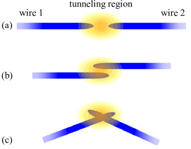
Figure 1: Shematic representation of three possible extended contact geometries.

II Model and formalism

We start by considering the one-dimensional (1D) tunnel junction for spinless electrons with Hamiltonian

$$H=H_{1}+H_{2}+H_{T}+H_{V},$$ (1)

where $H_{j}$ ($j=1,2$) describes the semi-infinite interacting wire $j$, $H_{T}$ the tunnel junction, and $H_{V}$ the applied bias voltage. The wires with interaction potential $U$ are modeled as open-boundary Tomonaga-Luttinger liquids according tounits

$$H_{j} = \frac{1}{2}\sum_{\alpha=R,L}[-2i\epsilon_{\alpha}v_{F}\int_{0}^{\infty}dx\,\psi^{\dagger}_{j\alpha}(x)\partial_{x}\psi_{j\alpha}(x)$$ (2)

$$+ \frac{1}{2}\int_{0}^{\infty}dx\,dy\,U(|x-y|)\rho_{j}(x)\rho_{j}(y)\,],$$

where $\alpha$ denotes the chirality of the electrons with Fermi velocity $\epsilon_{\alpha}v_{F}$ ($\epsilon_{R/L}=\pm 1$), $\psi^{(\dagger)}_{j\alpha}$ is the annihilation (creation) operator of one electron in wire $j$ and chirality $\alpha$ with density $\rho_{j}=\sum_{\alpha}:\psi^{\dagger}_{j\alpha}\psi_{j\alpha}:$, “$:\;\;:$” being the normal ordering. The junction between the two wires is modeled by the tunneling Hamiltonian

$$H_{T}=\sum_{\alpha,\alpha^{\prime}}\int_{0}^{\infty}dx\,dy\,\Gamma(x,y)\psi^{\dagger}_{1\alpha}(x)\psi_{2\alpha^{\prime}}(y)+\mathrm{h.c.},$$ (3)

where the function $\Gamma$ can eventually account for tunneling of electrons located not only at the boundaries of the wires. In the above expression it is understood that the tunneling amplitude $\Gamma$ depends on the distance between one point at position $x$ in wire $1$ and another point at position $y$ in wire $2$.

For latter purposes it is convenient to write $\Gamma(x,y)=\Gamma_{0}g(x,y)$ with $g$ an adimensional function encoding all the spatial dependence. The junction is driven out of equilibrium by an external voltage given by

$$H_{V}=\sum_{j}V_{j}\int dx\rho_{j}(x)=\sum_{j}V_{j}N_{j},$$ (4)

with $N_{j}=\sum_{\alpha}N_{\alpha j}$ the number of electrons in the wire $j$ and $V=V_{1}-V_{2}$ the total applied bias. The crucial quantity we are interested in is the tunneling current whose operator reads

$$J = \frac{dN_{1}}{dt}=-\frac{dN_{2}}{dt}$$ (5)

$$= i\sum_{\alpha,\alpha^{\prime}}\int_{0}^{\infty}dx\,dy\,\Gamma(x,y)\psi^{\dagger}_{1\alpha}(x)\psi_{2\alpha^{\prime}}(y)+\mathrm{h.c.}$$

Since we focus on the tunneling regime, in this work we evaluate the current to the second order in $\Gamma_{0}$. By employing the gauge transformationfeldman ; perfetto $\psi_{j\alpha}\to\psi_{j\alpha}e^{iV_{j}t}$ the steady-state average current $I=\langle J\rangle$ is (at zero temperature)

$$I = \frac{1}{4}\int_{-\infty}^{\infty}dt\,e^{iVt}\langle\Psi_{0}|[H_{T}(t),J(0)]|\Psi_{0}\rangle$$ (6)

$$\equiv \left(\frac{2\Gamma_{0}}{\pi a}\right)^{2}\int_{0}^{\infty}dx_{1}\ldots dx_{4}\,g(x_{12})g(x_{34})$$

$$\times \int_{-\infty}^{\infty}dt\,e^{iVt}e^{-W(t,\{x_{i}\})},$$

where $|\Psi_{0}\rangle$ is the interacting ground-state of the equilibrium uncontacted Hamiltonian $H_{1}+H_{2}$, and $H_{T}(t)$ and $J(0)$ are in Heisenberg representation with respect to $H_{1}+H_{2}$. In the above equation we have used the short-hand notation $x_{i,j}=(x_{i},x_{j})$ and $\{x_{i}\}=(x_{1},x_{2},x_{3},x_{4})$. The function $W$ is the equilibrium phase correlation function and its Fourier transform is related to the probability $P(E)$ for a tunneling electron of exchanging the energy $E$ with the bath of interacting electrons in the wires. It is explicitly given bysassetti1

$$P(E,\{x_{i}\})=\frac{1}{2\pi}\int_{-\infty}^{\infty}\,dEe^{iEt}e^{-[W(t,\{x_{i}\})-W_{0}(t,\{x_{i}\}]},$$ (7)

where $W_{0}$ is the correlation function of the corresponding noninteracting system.

The connection with the standard theory of CB is established by observing that the steady-state current of Eq. (6) can be rewritten as

$$I = \frac{8\Gamma_{0}^{2}}{\pi v_{F}}\int_{0}^{\infty}dx_{1}\ldots dx_{4}\,g(x_{12})g(x_{34})$$

$$\times \int_{-\infty}^{\infty}dEdE^{\prime}f(E)[1-f(E^{\prime})]P(E+V-E^{\prime},\{x_{i}\})$$

where $f(E)=1-\theta(E)$ is the zero-temperature Fermi function. For noninteracting electrons the tunneling becomes elastic, and $P(E,\{x_{i}\})=\delta(E)$ for every $\{x_{i}\}$, thus recovering the Ohmic $I$-$V$ curve $I\propto V$, as it should be. In the semiclassical approachtheor1 ; theor2 the function $P$ gives the probability of exchanging energy with the electromagnetic environment, which in the present microscopic theory is replaced by the bath of elementary excitations of the interacting quantum system.

The average in Eq. (6) can be evaluated by resorting the open-boundary bosonization method.obb1 ; obb2 ; obb3 It has been shown that the low-energy properties of the isolated semi-infinite wire $j$ with open boundary conditions can be described in terms of (say) right movers only which live in an infinite system without boundaries, and which are related to the left movers by the relation

$$\psi_{jL}(x)=\psi_{jR}(-x).$$ (8)

In the bosonization language the above relation implies that

$$\phi_{jL}(x)=\phi_{jR}(-x)+\mathrm{const},$$ (9)

where $\phi_{j\alpha}(x)$ is the boson field such that

$$\psi_{j\alpha}(x)=\frac{1}{\sqrt{2\pi a}}e^{-2\sqrt{\pi}\,i\epsilon_{\alpha}\phi_{j\alpha}(x)}\,e^{i\epsilon_{\alpha}k_{F}x},$$ (10)

where $k_{F}$ is the Fermi momentum and $a$ a short-distance cutoff. The great advantage of the bosonization technique is that the interacting ground-state appearing in Eq. (6) is nothing but the vacuum of the boson operators $b_{j\alpha q}$ entering in the mode expansion

$$\phi_{j\alpha}(x)=i\epsilon_{\alpha}\sum_{q>0}\frac{e^{-aq/2}}{\sqrt{2\mathcal{L}q}}[C_{q+}b_{j\alpha q}^{{\dagger}}-C_{q-}b_{j\bar{\alpha}q}]e^{-i\epsilon_{a}q}+\mathrm{h.c.},$$ (11)

where $\mathcal{L}$ is the length of the wires.nota The coefficients $C_{q\pm}$ carry all the information about the electron-electron interaction and are given by

$$C_{q\pm}=\frac{1\pm K_{q}}{2\sqrt{K_{q}}},$$ (12)

with $K_{q}=(1+\frac{U_{q}}{\pi v_{F}})^{-1/2}$, $U_{q}$ being the Fourier transform of $U(|x|)$. The special value $K_{0}\equiv K$ is the so-called LL parameter, and, as we shall see below, it governs the power-law behavior of the observables within the present theory.haldane

It is worth recalling that a single-channel conductor in series with a resistance $R$ can mimicsafi a LL with an impurity (or alternatively with a tunnel junction) and $K=(1+R/R_{0})^{-1}$. Therefore our theoretical treatment could also serve to describe mesoscopic resistive systems, see e.g. the recent experiment in Ref. exp12, , in which a LL with $K\approx 1/2$ was simulated.safi

III Point-like tunneling and interaction: CB regime

In this Section we briefly review the properties of a junction with point-like (edge-to-edge) tunneling $g(x,y)=\delta(x)\delta(y)$ and point-like (short-range) interaction $U(|x-y|)=U\delta(x-y)$ (i.e. $U_{q}=U$). In this case the function $W$ becomes particularly simple and it is given by

$$W(t)=\frac{2}{K}\log\frac{a+ivt}{a},$$ (13)

where $v=v_{F}(1+\frac{U}{\pi v_{F}})^{1/2}$ is the renormalized velocity. The temporal integral in Eq. (6) can be evaluated analytically and the steady-state current reads

$$I=\frac{8\Gamma_{0}^{2}\,V}{\pi v^{2}\Gamma(2/K)}\left(\frac{aV}{v}\right)^{2/K-2}.$$ (14)

This is the well-known result originally derived by Kane and Fisherkane by means of renormalization group arguments. For an arbitrary weak interaction the system becomes insulating, with the tunneling current suppressed (at zero temperature) as a power-law (CB regime). It is important to notice that, despite the power-law suppression of the current has been observed in several experiments, exp4 ; exp5 ; exp6 ; exp7 ; exp8 ; exp9 ; exp10 ; exp11 ; exp12 the above formula does not recover the SO behavior that must hold at large bias. In the following Section we show how this problem has been solved.

IV Finite-range interaction and point-like tunneling: SO regime

As anticipated in the Introduction, this case has been investigated in Ref. sassetti1, . Here we only summarize the main conclusions, assuming a screened interaction of the form $U(|x-y|)=\frac{U}{d}e^{-|x-y|/d}$. We stress, however, that the results do not depend on the explicit form of the interaction. The finite range of the interaction is encoded in the momentum-dependent functions

$$K_{q} = \left[1+\frac{U}{\pi v_{F}(1+q^{2}d^{2})}\right]^{-1},$$

$$v = v_{F}\left[1+\frac{U}{\pi v_{F}(1+q^{2}d^{2})}\right],$$ (15)

as well as in the charging energy of the junction $V_{d}=2U(0)=2U/d$. A small bias probes the low-energy (i.e. low-momentum $q$) excitations of the electron liquid, and hence in this regime the system behaves as the interaction was zero-range with $K_{q}\approx K=(1+\frac{U}{\pi v_{F}})^{-1}$. Accordingly for $V\ll V_{d}$ the same behavior $I\propto V^{2/K-1}$ as in Eq. (14) is found. A large bias, instead, probes high-$q$ excitations, for which $K_{q}\approx 1$ [see Eq. (15)], like in the non-interacting system. As a consequence the SO regime is correctly recovered, where the effects of correlation manifest in a shift in the $I$-$V$ curve $I\approx V/R_{T}-V_{d}$, where $R_{T}=8\Gamma_{0}^{2}/\pi v^{2}$ is the tunneling resistance of the junction. The crossover between the two regimes occurs at the critical voltage $V=V_{d}$. We would like to mention that it has been recently shown that the finite-range interaction is also at the origin of the current suppression at small $V$ in single-channel quantum dot tunnel junctions, whereas a point-like $U$ produces an Ohmic behavior.perfetto2

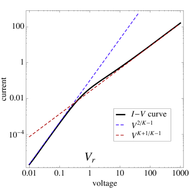
Figure 2: Log-log plot of the $I$-$V$ curve for extended tunneling with range $r=2\times 10^{5}a$ and point-like interaction with $U=6v_{F}$ (i.e. LL parameter $K\approx 0.6$). The dashed lines represent the two power-laws with different exponents holding for $V<V_{r}$ and $V>V_{r}$ ($V_{r}\approx 1$ in this figure). Voltages $V$ and $V_{r}$ are in units of $10^{-5}v_{F}/a$, and the current $I$ is in units of $10^{-5}\Gamma_{0}^{2}/av_{F}$.

V Finite-range tunneling and point-like interaction: ET regime

For illustration we consider a linear junction like the one in Fig. 1a. However, the explicit choice of the geometry cannot affect qualitatively the results. The finite-range tunneling amplitude is in this case $g(x,y)=e^{-(r_{0}+x+y)/r}$, where $r_{0}$ is the spatial separation between the edges of the wires,nota1 and $r$ is the size of the extended contact. We are aware that the most accurate form of the spatial-dependent tunneling amplitude $g$ is probably gaussian, since it is proportional to the overlap between states from the two sides of the junction.exttunn3 Nevertheless, we here prefer to adopt the same exponential function for both tunneling amplitude and interaction, in order make direct comparisons (see next Section). Since we can absorb the factor $e^{-r_{0}/r}$ into the value of $\Gamma_{0}$, we take $r_{0}=0$ without loss of generality. In this Section we first consider a point-like interaction $U_{q}=U$ which makes the calculation analytically tractable, thus allowing to get transparent formulas to disentangle the effects of ET. To simplify the calculations we approximate the integral in Eq. (6) as

$$I\approx\left(\frac{2\Gamma_{0}}{\pi a}\right)^{2}\int_{0}^{\infty}dx\,e^{-2x/r}j(x),$$ (16)

where $j(x)=\int_{-\infty}^{\infty}dt\,e^{iVt}e^{-W(t,x)}$ is the steady-state current of an effective junction in which the tunneling occurs only between the points at position $x$ in both wires. This means that we are assuming that the dominant contribution to the current comes from the tunneling events in which $x_{1}=x_{2}=x_{3}=x_{4}=x$.nota3 Within this approximation the function $j(x)$ can be evaluated analytically in the limits of small and large (compared to scale $V_{x}=v/x$) bias.

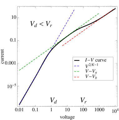
Figure 3: Log-log plot of the $I$-$V$ curve for extended tunneling and finite-range interaction for $V_{d}<V_{r}$. We used $r=2\times 10^{3}a$, $d=10^{6}a$, $U=6v_{F}$ (i.e. $K_{0}\approx 0.6$, $V_{r}\approx 100$ and $V_{d}\approx 1.2$). The dashed lines represent the three power-laws with different exponents holding for $V<V_{r}$, $V_{r}<V<V_{d}$ and $V>V_{r}$. Voltages and current are in the same units as in Fig. 2. In the legend $V_{a}$ and $V_{b}$ indicate the different offset of the two shifted Ohmic regimes.

At small bias $V\ll V_{x}$ the function $\mathrm{exp}[-W(t,x)]$ is dominated by the singularities around $t=\pm 2x/v$, yielding

$$j(x)\propto x^{1/K-K}V^{2/K-1}\quad\mathrm{for}\;V\ll V_{x}.$$ (17)

In the opposite limit the function $\mathrm{exp}[-W(t,x)]$ is instead dominated by the singularity around $t=0$, and the asymptotic current $j$ is independent on $x$,

$$j(x)\propto V^{K+1/K-1}\quad\mathrm{for}\;V\gg V_{x}.$$ (18)

The crossover between the two regimes occurs at bias $V\approx V_{x}$. In order to obtain the true tunneling current $I$, we have to integrate $j(x)$ according to Eq. (16). The numerical result is show in Fig. 2, where it is clearly seen that the crossover is also displayed by $I$ under the replacement $x\to r/2$ and $V_{x}\to V_{r}=2v/r$. The physical interpretation of this behavior is the following: For an edge-to-edge tunneling, the current is suppressed as $V^{2/K-1}$ [see Eq. (14)] due to the interaction-induced depletion of density of states in the proximity of the boundary;obb3 allowing electrons to tunnel over the depletion region, enhances the current according to a power-law with exponent $K+1/K-1<2/K-1$, provided that the energy supplied by the applied voltage is larger than the tunneling energy $\sim V_{r}$ (ET regime). In the next Section we will present the most important part of the paper, in which we consider the simultaneous effect of extended contacts and screened interaction. This will allow us to study the competition between the two energy scales $V_{d}$ and $V_{r}$, and see the impact on the CB scenario.

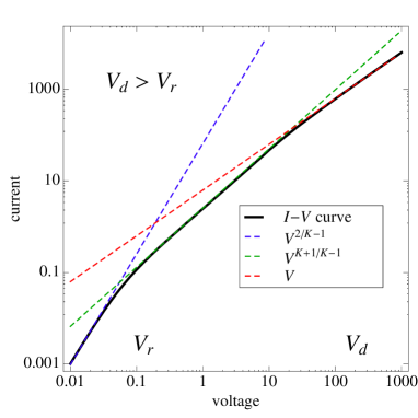
Figure 4: Log-log plot of the $I$-$V$ curve for extended tunneling and finite-range interaction for $V_{d}>V_{r}$. We used $r=2\times 10^{6}a$, $d=10^{4}a$, and $U=6v_{F}$ (i.e. $K_{0}\approx 0.6$, $V_{r}\approx 0.1$ and $V_{d}\approx 120$). The dashed lines represent the three power-laws with different exponents holding for $V<V_{r}$, $V_{r}<V<V_{d}$ and $V>V_{r}$. Voltages and current are in the same units as in Fig. 2.

VI Finite-range tunneling and interaction: Competition

We now consider the tunneling amplitude $g(x,y)=e^{-(x+y)/r}$ and the screened interaction $U(|x-y|)=\frac{U}{d}e^{-|x-y|/d}$. As noticed in Ref. vignale, the length scales $r$ and $d$ are typically of the same order, and hence it is important to treat their effects on the same footing. According to the results of the previous Sections, if the applied bias is smaller than $\min\{V_{r},V_{d}\}$ the system is certainly in the CB regime, with the current suppressed as $I\propto V^{2/K-1}$ (see Figs. 3 and 4 ). However, at larger bias the response crucially depends on the interplay between tunneling and screening.

VI.1 $V_{d}<V_{r}$

If $V_{d}<V_{r}$ a SO behavior (with offset $V_{a}$, see Fig. 3) is expected in the range $V_{d}<V<V_{r}$, since ET effects are still not significant. But what happens when $V>V_{r}$? Tunneling effects will compete with screening effects, compelling the system to abandon the Ohmic behavior and to crossover towards the power-law regime $I\sim V^{K+1/K-1}$. To understand the fate of such competition we have to calculate $I$ numerically. For simplicity we adopt the same approximation as in Eq. (16), and the resulting $I$-$V$ curve is shown in Fig. 3. We see that for $V>V_{r}$ no real crossover occurs, and the current remains Ohmic (there is a kink separating two different SO regimes). The physical reason of this behavior can be understood as follows: Since the interaction range is finite, for $V>V_{d}$ the system behaves as it was noninteracting, where the effects of interaction are only visible in the Coulomb offset of the linear $I$-$V$ curve; as a consequence, when $V>V_{r}$ tunneling effects are felt by a “noncorrelated state” having $K\approx 1$ and hence $I\propto V^{K+1/K-1}\approx V$. Indeed at $V\approx V_{r}$ a “transition” between two different Ohmic regimes (characterized by different offests $V_{a}$ and $V_{b}$) is observed, see the green and red dotted lines in Fig. 3. In conclusion for $V_{d}<V_{r}$ the ET regime characterized by $I\propto V^{K+1/K-1}$ is completely suppressed.

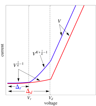
Figure 5: Schematic illustration of the renormalization of the Coulomb blockade gap $\Delta$. Red line: $I$-$V$ curve for a point-like (end-to-end) tunneling and finite-range interaction, with usual gap $\Delta\approx V_{d}\equiv\Delta_{d}$. Blue line: $I$-$V$ curve for extended tunneling and finite-range interaction with $V_{d}>V_{r}$. The Coulomb blockade gap renormalizes as $\Delta\approx V_{r}\equiv\Delta_{r}<\Delta_{d}$.

VI.2 $V_{d}>V_{r}$

If $V_{d}>V_{r}$ the analysis is simpler, but the scenario is more intriguing. In this case there is no real competition between ET and screening since $I\propto V^{K+1/K-1}$ develops in the range $V_{r}<V<V_{d}$ while the SO behavior naturally establishes in the “noncorrelated” regime at large bias $V>V_{d}$. Indeed in Fig. 4 we can observe the three different regimes displayed by the $I$-$V$ curve which has been calculated numerically. Remarkably the occurrence of the ET regime before the occurrence of the SO behavior causes a reduction of the CB gap, because $I$ is suppressed as $V^{2/K-1}$ only for $V<V_{r}$ (instead of $V<V_{d}$). Since the $K+1/K-1<2/K-1$ for any repulsive interaction, we conclude that beyond the threshold $V=V_{r}$ the current is enhanced according to a “weakly correlated” power-law (although the regime is still not completely Ohmic).

This finding may have relevant consequences from the experimental side, in particular for what concerns the estimate of the junction capacitance $C$. Indeed $C$ is usually inferred from the relation $1/2C=\Delta$, where $\Delta$ is the observed Coulomb blockade gap, identified as the high voltage offset of the $I$-$V$ curve.exp4 ; exp9 Our results point out that in situations in which the screening length is smaller than the spatial extension of the tunneling processes, the relation $\Delta\approx V_{d}$ must be replaced by $\Delta\approx V_{r}$ (for an illustration, see Fig. 5). This means that the observed gap is not simply equal to the conventional charging energy, but it is strongly renormalized by the energy that electrons need to tunnel over an extended region of size $v/\Delta$.

The novel regime we propose could be experimentally realized in tunnel junctions involving multiwall carbon nanotubes. These systems display a manifest LL behaviorexp9 ; egger and at the same time the screening by nearby gates (or substrate) and by the different shells renders the interaction short-ranged.egger ; egger2 Thus the condition $V_{d}>V_{r}$ can be effectively fulfilled, and extracting the value of the capacitance from the offset of the $I$-$V$ curve may provide a result significantly larger than the correct one.

VII Spinful case

So far we have considered spinless electrons. In this Section we introduce the spin degrees of freedom, and show that the above scenario survives also in this case. The formulation is very similar to the one presented in Section II. If the spin is taken into account the boson field $\phi_{j\alpha}$ introduced in Eqs. (9,10) becomes explicitly spin-dependent, which we denote by $\phi_{j\alpha\sigma}$, where $\sigma=\uparrow,\downarrow$ is the spin orientation. If the interaction does not depend on the spin of the scattering electrons [i.e. $U_{\sigma\sigma^{\prime}}(x)=U(x)$] it is useful to introduce the charge/spin fields $\phi_{j\alpha c/s}=(\phi_{j\alpha\uparrow}\pm\phi_{j\alpha\downarrow})/\sqrt{2}$. In terms of these new fields the original spinful Hamiltonians separateshaldane in an interacting part in the charge sector characterized by LL parameter $K_{c}$ and velocity $v_{c}$ (which is equivalent to the one of the interacting spinless case) and a noninteracting part in the spin sector with $K_{s}=1$ and $v_{s}=v_{F}$. The calculation of the current follows the same line as above, with the only difference that in this case the interacting ground-state $|\Psi_{0}\rangle$ is (in the bosonization language) the product of the vacua of the charge and spin excitations respectively. It is straightforward to verify that the competition between the ET regime and the SO regimes takes place as above, but with different power-law exponents: $I\propto V^{1/K_{c}}$ in the CB regime and $I\propto V^{(K_{c}+1/K_{c})/2}$ in the ET regime. Again it holds $1/K_{c}>(K_{c}+1/K_{c})/2$ (for any repulsive interaction), thus ensuring the renormalization of the CB gap also for spinful electrons. Finally we have verified that in this case the relevant energy scales are $V_{d}=v_{c}/d$ and $V_{r}=v_{c}/r$, i.e. both the charging energy and the ET energy depend only on the velocity of charge excitations, as it should be.

VIII Summary and conclusions

We have investigated the zero-temperature nonequilibrium transport properties of a nanoscopic junction formed by two single-channel conductors linked by an extended contact. We have considered the simultaneous effect of finite-range electron-electron interaction and extended tunneling, by paying special attention to the Coulomb blockade phenomenon. Correlations have been included within the open-boundary Luttinger liquid theory, while tunneling processes have been treated to linear order in the tunneling Hamiltonian. Two relevant length scales enter in the problem, namely the screening length $d$ and the size of the extended contact $r$, and different scenarios have been discussed depending on their relative magnitude. When $d$ and $r$ are comparable a competition between screening and tunneling occurs, opening the possibility of identifying a new regime. In particular when $d<r$ a “weakly correlated” regime at intermediate voltage $V$ establishes between the well-known Coulomb blockade regime (holding at small $V$) and the shifted Ohmic regime (holding at large $V$). This produces an increase of the tunneling current from the CB suppression $I\sim V^{2/K-1}$ to the enhanced power-law $I\sim V^{K+1/K-1}$. As a consequence the CB gap shrinks from the “electrostatic” value $\Delta\sim 2U(0)$ to the renormalized value $v/r$, which is not the charging energy of the junction, but it is rather the energy that must be supplied to a single electron to tunnel over an extended region of size $r$. Finally we have shown that the above results are robust with respect to the introduction of the spin degrees of freedom, whose effect consists in modification of the power-law exponents in the CB and ET regimes.

References

- (1) D. V. Averin and K. K. Likharev, Mesoscopic Phenomena in Solids (Elsevier, Amsterdam, 1991).
- (2) H. Grabert and M. H. Devoret, Single Charge Tunneling: Coulomb Blockade Phenomena in Nanostructures (Plenum, New York, 1992).
- (3) Through this paper we use .
- (4) P. J. M. van Bentum, H. van Kempen, L. E. C. van de Leemput, and P. A. A. Teunissen, Phys. Rev. Lett. 60, 369 (1988).
- (5) R. Wilkins, E. Ben-Jacob, and R. C. Jaklevic, Phys. Rev. Lett. 63, 801 (1989).
- (6) L. J. Geerligs, V. F. Anderegg, P. A. M. Holweg, J. E. Mooij, H. Pothier, D. Esteve, C. Urbina, and M. H. Devoret, Phys. Rev. Lett. 64, 2691 (1990).
- (7) A. N. Cleland, J. M. Schmidt, and John Clarke, Phys. Rev. Lett. 64, 1565 (1990); Phys. Rev. B 45, 2950 (1992).
- (8) T. Holst, D. Esteve, C. Urbina, and M. H. Devoret, Phys. Rev. Lett. 73, 3455 (1994).
- (9) F. Pierre, H. Pothier, P. Joyez, Norman O. Birge, D. Esteve, and M. H. Devoret, Phys. Rev. Lett. 86, 1590 (2001).
- (10) D. S. Golubev and A.D. Zaikin, Phys. Rev. Lett. 86, 4887 (2001).
- (11) A. Levy Yeyati, A. Martin-Rodero, D. Esteve, and C. Urbina, Phys. Rev. Lett. 87, 046802 (2001).
- (12) R. Tarkiainen, M. Ahlskog, J. Penttilä, L. Roschier, P. Hakonen, M. Paalanen, and E. Sonin, Phys. Rev. B 64, 195412 (2001).
- (13) W. Yi, L. Lu1, H. Hu, Z. W. Pan, and S. S. Xie, Phys. Rev. Lett. 91, 076801 (2003)
- (14) C. Altimiras, U. Gennser, A. Cavanna, D. Mailly, and F. Pierre, Phys. Rev. Lett. 99, 256805 (2007).
- (15) F. D. Parmentier, A. Anthore, S. Jezouin, H. le Sueur, U. Gennser, A. Cavanna, D. Mailly, and F. Pierre, Nature Physics 7, 935 (2011).
- (16) C. Brun, K. H. Müller, I-P. Hong, F. P., C. Flindt, and W-D. Schneider, Phys. Rev. Lett. 108, 126802 (2012).
- (17) M. H. Devoret, D. Estève, H. Grabert, G.-L. Ingold, H. Pothier, and C. Urbina, Phys. Rev. Lett. 64, 1824 (1990).
- (18) G.-L. Ingold and Yu.V. Nazarov, in Charge Tunneling Rates in Ultra- small Junctions, B294, H. Grabert and M.H. Devoret Eds. (Plenum Press, New York, 1992), Chap. 2, p. 21.
- (19) M. Sassetti, G. Cuniberti and B. Kramer, Sol. St. Comm. 101, 915 (1997).
- (20) M. Sassetti and B. Kramer, Phys. Rev. B 55, 9306 (1997).
- (21) M. Steiner and W. Häusler, Sol. St. Comm. 104, 799 (1997).
- (22) E. B. Sonin, J. Low Temp. Phys. 1, 321 (2001).
- (23) I. Safi and H. Saleur, Phys. Rev. Lett. 93, 126601 (2004).
- (24) C. L. Kane and M. P. A Fisher, Phys. Rev. Lett. 68, 1220 (1992); Phys. Rev. B 46, 15233 (1992).
- (25) M. Bockrath, D. H. Cobden, J. Lu, A. G. Rinzler, R. E. Smalley, L. Balents, and P. L. McEuen, Nature (London) 397, 598 (1999).
- (26) Z. Yao, H. W. C. Postma, L. Balents, and C. Dekker, Nature (London) 402, 273 (1999).
- (27) M. Aranzana, N. Regnault, and T. Jolicoeur, Phys. Rev. B 72, 085318 (2005).
- (28) I.Safi, arXiv:0906.2363.
- (29) B. J. Overbosch and C. Chamon, Phys. Rev. B 80, 035319 (2009).
- (30) D. Chevallier, J. Rech, T. Jonckheere, C. Wahl, and T. Martin, Phys. Rev. B 82, 155318 (2010).
- (31) D. S. Golubev, A. D. Zaikin, Phys. Rev. B 85, 125406 (2012).
- (32) G. Dolcetto, S. Barbarino, D. Ferraro, N. Magnoli, and M. Sassetti, arXiv:1203.4486.
- (33) R. D’Agosta, G. Vignale, and R. Raimondi, Phys. Rev. Lett. 94, 086801 (2005).
- (34) D. E. Feldman and Y. Gefen, Phys. Rev. B 67, 115337 (2003).
- (35) E. Perfetto, G. Stefanucci, and M. Cini, Phys. Rev. Lett. 105, 156802 (2010).
- (36) M. Fabrizio and A. O. Gogolin, Phys. Rev. B 51, 17827 (1995).
- (37) S. Eggert, H. Johannesson, and A. Mattson, Phys. Rev. Lett. 76, 1505 (1996).
- (38) S. Eggert, Phys. Rev. Lett. 84, 4413 (1999).
- (39) At the end of the calculation of any boson average the length must be sent to infinity, by remembering that .
- (40) F. D. M. Haldane, J. Phys. C 14, 2585 (1981).
- (41) E. Perfetto, G. Stefanucci, and M. Cini Phys. Rev. B 85, 165437 (2012).
- (42) R. Zamoum, A. Crépieux, and I. Safi, Phys. Rev. B 85, 125421 (2012).
- (43) If the ending points of the two wires are separated by a distance , the distance between and is , since in both wires positions are positive definite, see Eqs. (2,3).
- (44) The evaluation of the full integral in Eq. (6) is computationally very demanding, but provides results in good agreement with the approximated expression in Eq. (16), due to the strong peaked shape of the correlators like around .
- (45) R. Egger, Phys. Rev. Lett. 83, 5547 (1999).
- (46) R. Egger and A. O. Gogolin, Chem. Phys. 281, 447 (2002).