Bulk flow of halos in $\Lambda$CDM simulation

Abstract

Analysis of the Pangu $N$-body simulation validates that the bulk flow of halos follows a Maxwellian distribution which variance is consistent with the prediction of the linear theory of structure formation. We propose that the consistency between the observed bulk velocity and theories should be examined at the effective scale of the radius of a spherical top-hat window function yielding the same smoothed velocity variance in linear theory as the sample window function does. We compared some recently estimated bulk flows from observational samples with the prediction of the $\Lambda$CDM model we used; some results deviate from expectation at a level of $\sim 3\sigma$ but the discrepancy is not as severe as previously claimed. We show that bulk flow is only weakly correlated with the dipole of the internal mass distribution, the alignment angle between the mass dipole and the bulk flow has a broad distribution peaked at $\sim 30-50^{\circ}$, and also that the bulk flow shows little dependence on the mass of the halos used in the estimation. In a simulation of box size $1h^{-1}$Gpc, for a cell of radius $100^{-1}$Mpc the maximal bulk velocity is $>500{\rm km}\,{\rm s}^{-1}$, dipoles of the environmental mass outside the cell are not tightly aligned with the bulk flow, but are rather located randomly around it with separation angles $\sim 20^{\circ}$–$40^{\circ}$. In the fastest cell there is a slightly smaller number of low-mass halos; however halos inside are clustered more strongly at scales $\gtrsim 20h^{-1}$Mpc, which might be a significant feature since the correlation between bulk flow and halo clustering actually increases in significance beyond such scales.

1. Introduction

Bulk flow refers to the apparent coherent peculiar motion of galaxies and galaxy clusters in a considerably large volume around us. In practice there are several ways to estimate bulk flows from various observation resources, such as galaxy catalogs from peculiar velocity surveys (e.g. Feldman et al., 2010), compiled Type Ia supernovae data (e.g. Dai et al., 2011), and galaxy clusters in combination with cosmic microwave background (CMB) observations (e.g., Kashlinsky et al., 2010). Recently some interesting new methods based on galaxy two-point correlation functions (Song et al., 2011) and galaxy light (Nusser et al., 2011; Abate & Feldman, 2012) have also emerged.

Analysis of the spiral galaxy catalog of the SFI++ survey (Springob et al., 2007) shows that within a top-hat spherical window of radius $40h^{-1}$Mpc the velocity of the bulk flow is $338\pm 38{\rm km}\,{\rm s}^{-1}$ toward Galactic plane $(l,b)=(276^{\circ},14^{\circ})$ with a $3^{\circ}$ $1\sigma$ uncertainty, and then $257\pm 44{\rm km}\,{\rm s}^{-1}$ toward $(l,b)=(279^{\circ},10^{\circ})$ with a $6^{\circ}$ error within window of radius $100h^{-1}$Mpc (Nusser & Davis, 2011). These measurements are in agreement with the analysis by Sandage et al. (2010) of data consisting of supernovae, selected nearby galaxies, and galaxy clusters. Feldman et al. (2010) constructed a composite catalog of galaxies with peculiar velocities measured in different surveys, including the SFI++. They estimate that the bulk flow within a Gaussian window of $50h^{-1}$Mpc is $416\pm 78{\rm km}\,{\rm s}^{-1}$ in the direction $(l,b)=(282\pm 11^{\circ},6\pm 6^{\circ})$ (see also Watkins et al., 2009).

Employing the peculiar velocities of supernovae is another viable route to detect bulk flow, though such samples are usually very sparse and prone to Malmquist bias. Dai et al. (2011) fitted a bulk flow of $188^{+119}_{-103}{\rm km}\,{\rm s}^{-1}$ in the direction $(l,b)=({290^{+39}_{-31}}^{\circ},{20^{+32}_{-32}}^{\circ})$ to the Union2 supernovae catalogue (Amanullah et al., 2010) for redshifts $z<0.05$, but no significant bulk flow was detected from data at $z>0.05$. Colin et al. (2011) used the same data to obtain a similar estimate but with a higher median amplitude of $250^{+190}_{-160}{\rm km}\,{\rm s}^{-1}$. However, using a different supernovae data set within the redshift shell $z=(0.0043,0.028)$, Weyant et al. (2011) estimate that the local flow is $538\pm 86{\rm km}\,{\rm s}^{-1}$ pointing to $(l,b)=(258^{\circ}\pm 10^{\circ},36^{\circ}\pm 11^{\circ})$, or $446\pm 101{\rm km}\,{\rm s}^{-1}$ towards $(l,b)=(273\pm 11^{\circ},46\pm 8^{\circ})$ if a different technique is employed, this is in agreement with the dipole of the CMB $(l,b)=(263^{\circ}.99\pm 0^{\circ}.14,48^{\circ}.26\pm 0^{\circ}.03)$ (Jarosik et al., 2011). Jha et al. (2007) and Haugbølle et al. (2007) have found the same values with similar uncertainties.

The availability of recent galaxy peculiar velocity data is limited to our local universe; the bulk flow at higher redshift, sometimes dubbed dark flow, is mainly explored through the kinetic Sunyaev–Zel’dovich (kSZ) effect of galaxy clusters (Sunyaev & Zeldovich, 1980). Kashlinsky et al. (2011) computed kSZ signals of 771 X-ray clusters in the 7 yr Wilkinson Microwave Anisotropy Probe (WMAP) CMB map, and conclude that the flow at $z\leq 0.16$ is directed to $(l,b)=(278\pm 18^{\circ},2.5\pm 15^{\circ})$ and then $(l,b)=(283\pm 19^{\circ},20\pm 15^{\circ})$ if $z\leq 0.25$. They further argue that the flow at these depths shall reach magnitude of $\sim 1000{\rm km}\,{\rm s}^{-1}$ according to an earlier investigation in Kashlinsky et al. (2010). Osborne et al. (2011) derived a conflicting assertion from the same CMB map in conjunction with 736 ROSAT observed clusters: that there is no significant detection of kSZ effects at low multipoles, basically denying the existence of bulk flow. In some cases, however, the thermal Sunyaev-Zel’dovich effect might induce a dipole that could easily be misunderstood as bulk flow of $\sim 2000-4000{\rm km}\,{\rm s}^{-1}$.

Bulk flow is a topic of long-term interest to observational cosmology (see Strauss & Willick, 1995, for a review of early works), and special surveys have been dedicated to it (e.g. Courtois et al., 2011). However, as we see, no consensus on the amplitudes, directions, or convergence depth of bulk flows has yet been achieved to reconcile different measurements. Nonetheless, some authors have argued that the amplitude of their measured bulk flow is too strong over such large scales, presenting a challenge to the standard $\Lambda$CDM model, or at least to that of the 5yr WMAP parameters (Watkins et al., 2009; Kashlinsky et al., 2010; Feldman et al., 2010; Macaulay et al., 2011). Not surprisingly, cosmological models of different flavors have been constructed to explain such anomalies (e.g., Mersini-Houghton & Holman, 2009; Afshordi et al., 2009; Wyman & Khoury, 2010), but new analysis of similar data sets seems to have nullified support for such a violation (Turnbull et al., 2012; Ma & Scott, 2012).

Expectation about bulk flow in $\Lambda$CDM universe is generally calculated with linear perturbation theory of large scale structure in that at large scales its accuracy is believed sufficient. Often the 1-D velocity variance of dark matter are quoted to compare with measurements, however we need to address here that it is the rms velocity that should be used instead of the 1-D rms velocity. (Mak et al., 2011) calculated that by linear theory the rms bulk velocity is typically $\sim 300{\rm km}\,{\rm s}^{-1}$, and claimed that uncertainty at $95\%$ confidence due to sample variance is approximately $200{\rm km}\,{\rm s}^{-1}$ for a top-hat window of radius $60h^{-1}$Mpc (Mak et al., 2011). A concern is that non-linearity might not be negligible even at very large scales (e.g. Scoccimarro, 2004), which could act as systematical bias to the conclusion about the consistency between model and data.

Although linear theory can predict the possibility of observing a bulk flow of particular amplitude at certain scale, several key problems yet can not be easily tackled analytically, e.g. internal properties of the volume demonstrating large bulk blow. Practically halo catalogues from N-body simulation in large box with sufficient mass resolution are best suited for such task. The reason of focusing on halos instead of dark matter is that observational objects used to determine bulk flow are galaxies and galaxy clusters which are residing in halos, and in practice the strongly non-linearity of peculiar velocities of galaxies is largely filtered out so that what contribute to bulk flow estimation is mainly the motion following their host halos (e.g. Watkins et al., 2009). In fact Bahcall et al. (1994) and Moscardini et al. (1996) have performed analysis of mock halo catalogues and obtained useful results, but their simulations are either of very low mass resolution or based on compromised simulation method. In this paper we will demonstrate our analysis of the velocity field of halos resolved from a dark matter only $\Lambda$CDM simulation in $1h^{-1}$Gpc box with $3072^{3}$ particles. The large volume and high mass resolution of our simulation enables investigating halo behaviors in detail over broad dynamic ranges superseding previous works.

In section 2 definition and basic theoretical prediction of bulk flow is introduced, which is followed by section 3 presenting measurements of bulk flow of randomly placed cells in simulation. Section 4 is devoted to analysis of special regions showing extraordinarily large bulk flow velocity. Summary and discussion is in the last section.

2. Bulk flow in linear theory

Placing a window of characteristic scale $R$ randomly in the sample space, if $N$ objects (galaxies, galaxy clusters or halos, in this work just the latter) are enclosed, bulk flow of the particular volume indicated by the particular object is

$$\mathbf{V}=\sum_{i=1}^{N}w_{i}\mathbf{v}_{i}/\sum w_{i}\ ,$$ (1)

in which $\mathbf{v}_{i}$ is the peculiar velocity of the $i$th object and $w_{i}$ is the weight assigned. Practically the weights could be originated from radial selection function, angular selection function (survey mask), luminosity, mass and etc.

2.1. Sample window

Effect of the sample window is pure geometrical, which can be easily modeled, In continuous limit, Eq. 1 becomes

$$\mathbf{V}=\mathbf{v}\otimes W(R)=\int\mathbf{v}(\mathbf{r})W(\mathbf{r};R){\rm d}r^{3}=\frac{1}{(2\pi)^{3}}\int\mathbf{v}(\mathbf{k})\widetilde{W}{\rm d}^{3}k\ ,$$ (2)

where $W(\mathbf{r};R)$ is the window function of characteristic scale $R$ evaluated at position vector $\mathbf{r}$ and $\widetilde{W}$ is its Fourier transformation. In principle $W$ could be anisotropic, e.g. due to incomplete sky coverage and non-uniform depth. The simplest and mostly common are the spherical top-hat window $\widetilde{W}_{th}=3(\sin kR-kR\cos kR)/(kR)^{3}$ and Gaussian window $\widetilde{W}_{G}=\exp(-k^{2}R^{2}/2)$, in fact there are little differences among top-hat, Gaussian and anisotropic windows in for bulk flow statistics if effective scale has been taken care of. Sometimes bulk flow estimation is provided by objects within a spherical shell defined by two radius $R_{1}>R_{0}$, it is easy to see that Eq. 2 applies with window function $\widetilde{W}_{S}=(R_{1}^{3}\widetilde{W}_{1}-R_{0}^{3}\widetilde{W}_{0})/(R_{1}^{3}-R_{0}^{3})$.

Probability distribution function (PDF) of $\mathbf{V}$ could be expressed as

$$p(\mathbf{V}){\rm d}\mathbf{V}=p(V){\rm d}Vp(\hat{n}_{V}){\rm d}\hat{n}_{V}$$ (3)

where $\hat{n}_{V}$ denotes the unit vector in direction of the bulk velocity. Isotropic assumption leads to $p(\hat{n}_{V})=1/4\pi$ and $\langle\hat{n}_{V}\rangle=0$, which ensures that $\langle\mathbf{V}\rangle=\int Vp(V){\rm d}V\int\hat{n}_{V}p(\hat{n}_{V}){\rm d}\hat{n}_{V}=\langle V\rangle\cdot\langle\hat{n}_{V}\rangle=0$. Integration over the angular part of Eq. 3 yields the PDF of the amplitude of bulk flow

$$p(V){\rm d}V=\left[\int p(\mathbf{V}){\rm d}\hat{n}_{V}\right]V^{2}{\rm d}V=4\pi p(\mathbf{V})V^{2}{\rm d}V\ .$$ (4)

$\mathbf{V}$ by definition is the velocity field smoothed by the window function, once the smoothing scale is sufficiently large the distribution of $\mathbf{V}$ shall be very close to Gaussian so that Maxwellian distribution could be invoked to model $p(V)$ (Bahcall et al., 1994)

$$p(V)dV=\sqrt{\frac{2}{\pi}}\left(\frac{3}{\sigma_{V}^{2}}\right)^{3/2}V^{2}\exp\left(-\frac{3V^{2}}{2\sigma_{V}^{2}}\right){\rm d}V\ ,$$ (5)

where the variance of $V$ can be obtained with $P_{\mathbf{v}\mathbf{v}}$, the power spectrum of $\mathbf{v}$, through

$$\sigma_{V}^{2}=\frac{1}{(2\pi)^{3}}\int P_{\mathbf{v}\mathbf{v}}{\widetilde{W}}^{2}{\rm d}^{3}k\ .$$ (6)

Given that radius of the window function $W(R)$ deployed to measure bulk flow is fairly large, one would expect that the velocity field smoothed at such scale will be well described by linear evolution of the initial condition, then if the initial distribution of velocity is Gaussian, for instance in the case of our simulation, Eq. 5 shall be a good approximation to the PDF of amplitudes of bulk flows. With the model, the most likely amplitude of bulk flow is simply $V_{p}=\sqrt{2/3}\sigma_{V}$, which ranges of variance corresponding to different levels can be computed by the integral

$$\int p(V){\rm d}V={\rm erf}\left(\sqrt{\frac{3V^{2}}{2\sigma_{V}^{2}}}\right)-\sqrt{\frac{6V^{2}}{\pi\sigma_{V}^{2}}}\exp\left(-\frac{3V^{2}}{2\sigma_{V}^{2}}\right)\ .$$ (7)

If $\mathbf{v}$ is curl free, a velocity potential field can be defined as $\theta(\mathbf{r})=-\nabla\cdot\mathbf{v}/(Haf)$ with the scale factor $a=1/(1+z)$, $f\equiv{\rm d}\log D(a)/{\rm d}\log a\approx\Omega_{m}^{4/7}+(1+\Omega_{m}/2)\Omega_{\Lambda}/70$ and $D(a)$ is the linear density growth factor at redshift $z=1/a-1$ (Lahav et al., 1991) , we have

$$\sigma^{2}_{V}=\frac{(Haf)^{2}}{(2\pi)^{3}}\int\frac{P_{\theta\theta}}{k^{2}}\widetilde{W}^{2}{\rm d}^{3}k\ .$$ (8)

The above expression relies on the assumption of negligible rotational velocity. In the linear regime, if the biasing of halo velocity to dark matter velocity is unity, it can be further simplified with the approximation $P_{\theta\theta}\approx P_{\delta\delta}^{(L)}$ where $P_{\delta\delta}^{(L)}$ is the linear matter power spectrum.

2.2. Selection function

In reality large fraction of galaxy samples are magnitude-limited (or flux-limited), galaxies fainter than certain threshold are missed in the sample, so that number density of observed galaxies $n(r)$ as function of distance to the observer, termed as radial selection function, is not constant. In the presence of selection function, if no correction is made, the measured bulkfow local to an observer is

$$\mathbf{V}=\frac{\int\mathbf{v}(\mathbf{r})n(r)W(\mathbf{r};R){\rm d}^{3}r}{\int n(r)W(\mathbf{r};R){\rm d}^{3}r}\ ,$$ (9)

in which $n(r)$ acts as the weighting function. In theoretical modeling Eq. 9 is equivalent to Eq. 2 if a new window function is defined through $W_{O}=n(r)W/\int nW{\rm d}^{3}r$, however there is still the conceptual difference of applying selection function than a pure geometrical window function. A non-constant selection function reflects the fact that the sampling to the velocity field is distance dependent; a window function not of top-hat type rather simply denotes that in the estimation the velocity field is weighted by a particular scheme, but the sampling to the field is fair.

The simplest proposal to correct the unfair sampling rate depicted by the selection function is to divide the measured peculiar velocity of an object by the selection function,

$$\hat{\mathbf{V}}=\frac{\sum_{i}^{N}w_{i}\mathbf{v}_{i}/n(r_{i})}{\sum_{i}^{N}w_{i}/n(r_{i})}\ ,$$ (10)

we will check its performance numerically later in this report (subsection 3.3).

Note that the discussion here is also applicable to the angular selection function which is termed as the completeness mask defined as the ratio of number of observed objects to the local observable number of that type of objects.

2.3. Physical Weights

Another type of weights different to selection functions is coming from physical properties of astronomical objects, such as mass, luminosity, internal velocity dispersion and etc. This kind of weights can not be assimilated into the sample geometrical window function in theoretical works, instead we have to develop statistical models to account for effects of these weighting schemes which often involves calculation of series of correlation between peculiar velocity and object’s physical quantities. Among the various physical weights, probably the most commonly seen is the mass. Mass may not always be the dominant actor determining properties of galaxies and clusters, but is always a major facotr. For example, for galaxies in some bands their luminosity-mass relation is considerably tight, weighting by luminosity could be deemed roughly equivalent to the weighting by certain power of mass. So later in this paper we will back to the issue of bulk flow weighted by mass, with a demonstrative numerical analysis (subsection 3.4).

3. Bulk flow shown in the Pangu simulation

3.1. The Pangu simulation and its halo catalogue

The Pangu simulation (PS-I) is a large volume and high resolution simulation, carried out under the scheme of the Computational Cosmology Consortium of China (dubbed C4). PS-I assumes a $\Lambda$ cold dark matter ($\Lambda$CDM) cosmology model with parameters

$$\Omega_{m}=\!0.26,\;\Omega_{b}=0.044,\;\Omega_{\Lambda}=0.74,$$

$$h=0.71,\;\sigma_{8}=0.8,\;n_{s}=1\ .$$

The simulation contains dark matter only, and uses $N=3,072^{3}$ particles to follow the distribution and evolution of dark matter within a periodic box with $L=1000h^{-1}$Mpc on a side. Each particle has a mass of $2.48915\times 10^{9}h^{-1}M_{\odot}$. The Plummer-equivalent force softening length is kept constant of $7h^{-1}$kpc.

The PS-I starts from redshift $z_{init}=127$, initial positions and velocities of particles is generated with Zel’dovich approximation from a glass-like particle set. Input linear power spectrum is computed with the CAMB (Lewis et al., 2000). The simulation is then run with L-GADGET, a memory-optimized version of GADGET2 (Springel, 2005). L-GADGET2 is designed to meet requirements of high performance computations, only the tree-particle mesh algorithm is included to calculate the gravitational forces efficiently. Totally 64 snapshots are saved from $z_{init}=127$ to redshift $z=0$. The PS-I is performed on the supercomputer Lenovo Deepcomp7000 at Supercomputing Center of Chinese Academy of Sciences. We use 2048 cores and about 6TB memory at the peak time. The simulation consumes approximately $6.5\times 10^{5}$ CPU hours (about 13 days) in total and consists of 6151 time steps.

Dark matter halos are identified on the fly during the simulation for each snapshot, using the standard friends-of-friends (FOF) algorithm with linking length of 0.2 times the mean particle separation. Each FOF group must contain at least 20 particles, at redshift $z=0$ there are $4.2\times 10^{7}$ identified particle groups. There are a little bit of ambiguity in definition of halo mass. Halo mass mostly used in literature is defined as the mass enclosed by a sphere centered on the halo center with certain radius, within which the average density is some factor larger than the critical density. A more convenient definition of halo mass is the total mass of all member particles of the FoF group, which is used in this paper. For simplicity the average of velocities of member particles are taken as the velocity of the halo.

In this work we used a subset of the group catalogue as our full halo catalogue, which consists of FoF groups of mass larger than $2.5\times 10^{11}h^{-1}M_{\odot}$ only and makes $1.28\times 10^{7}$ entries in the end. Selected FoF groups contains at least 100 member particles, corresponding Poisson fluctuation is greater than $10$ which is the threshold used for FoF group identification, limiting discreteness error to $10\%$ level. Another reason is that it is not easy to detect large number of low mass halos in observation. Our prudence test verifies that including FoF groups with number of particle $<100$ does not make any significant amendment to final results, even though effects of non-linearity are stronger. More importantly we will show that statistics of bulk flow are not sensitive to the mass of halos in the sample (subsection 3.5).

3.2. The probability distribution function of bulk flow

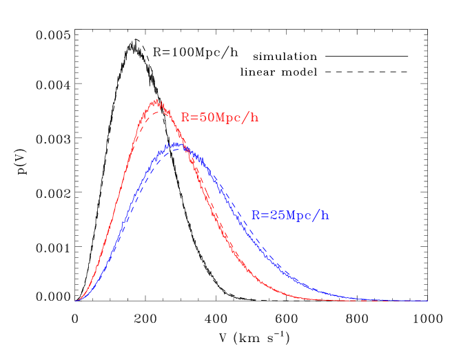
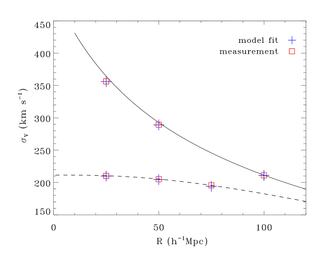
Figure 1.— Left panel: $p(V)$ measured in spherical top-hat windows with different radius, solid lines are measurements from N-body simulation, from left to right with decreasing heights corresponds to radius of window function $R=100,50,25h^{-1}$Mpc respectively, dashed lines are prediction of the model of Eq. 5 &  8 with $P_{\theta\theta}=P_{\delta\delta}^{(L)}$. Middle panel: $p(V)$ measured in one spherical shell window defined by two radius $(R_{0},R_{1})=(25,100)h^{-1}$Mpc. Right panel: comparison of $\sigma_{V}$ predicted by the linear theory (solid line is of spherical top-hat window, dashed line is of spherical shell window with $R_{0}=R$, $R_{1}=100h^{-1}$Mpc) with estimation from simulation (blue crosses), and the $\sigma_{V}$ which provide the best fitting to PDFs of bulk flow in simulation with Eq. 5 (red squares).

To ensure fair sampling to the simulation, the over-sampling algorithm of Szapudi (1998) is implemented to generate $\sim 10^{6}$ cells for $R$ within $25-100h^{-1}$Mpc, bulk flows of halos in random cells are estimated with Eq. 1. In our measurements we adopt mainly the spherical top-hat window, i.e. $w=1$ for all halos inside window and $w=0$ otherwise, meanwhile shell window function is also deployed for consistency check. Adopting the type of top-hat window function is just to simplify computation, in principle one could try Gaussian or other more sophisticated window functions, but it will not introduce change to the main results. Since our simulation box is limited in a cubic box of side length $1h^{-1}$Gpc, probe of bulk flows in cells of radius $>100h^{-1}$Mpc would be statistically unreliable.

Our measurements of bulk flows are displayed in Figure 1. For top-hat window, $\sigma_{V}$ decreases with cell radius, the possibility of finding extremely large speed of bulk flow becomes smaller for larger volume. For shell window defined by two radius $R_{0}<R_{1}$, if $R_{0}$ is not very close to $R_{1}$, $\sigma_{V}(R_{0},R_{1})\sim\sigma_{V}(R_{1})$.

More importantly, PDFs of amplitude of bulk flow in simulation, no matter measured with spherical top-hat window or spherical shell window, are all well described by the linear model. Agreement between simulation and model is better for larger volume as expected, linear theory slightly over-predicts $\sigma_{V}$ since nonlinear $P_{\theta\theta}$ is lower than $P_{\delta\delta}^{(L)}$ at $k\sim 0.1h{\rm Mpc}^{-1}$ by $\sim 20\%$ already (Nusser et al., 1991; Ciecielg & Chodorowski, 2004; Scoccimarro, 2004). The comparison clearly lead to the conclusion that to a good precision $p(V)$ obeys Maxwellian distribution which is completely determined by $\sigma_{V}$, what really matters is not the exact shape of the widow function but rather the corresponding $\sigma_{V}$. This lays out the solid ground for us to put different kinds of measurement together for comparison.

3.3. The simple correction for selection function

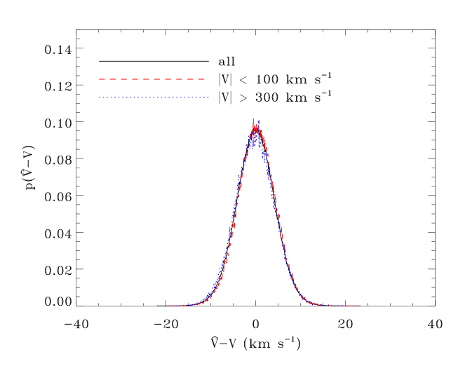
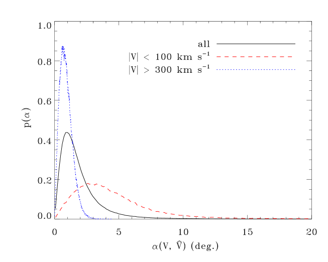
Figure 2.— Effectiveness of the correction for the selection function. $\hat{\mathbf{V}}$ is the corrected estimation (Eq. 10) to bulk flow with selection function applied, $\mathbf{V}$ is the normal one without selection function. Left: the relative difference between $p(\hat{V})$ and $p(V)$. Middle: PDFs of amplitude difference between $\mathbf{V}$ and $\hat{\mathbf{V}}$ in the same cell. Right: distribution functions of the angle between $\mathbf{V}$ and $\hat{\mathbf{V}}$ in the same cell, $\alpha=\cos^{-1}[\mathbf{V}\cdot\hat{\mathbf{V}}/(V\hat{V})]$. In the middle and the right panels also shown are subsamples of $V<100{\rm km}\,{\rm s}^{-1}$ (red dashed line) and $V>300{\rm km}\,{\rm s}^{-1}$ (blue dotted line).

In this part we take numerical approach to assess effectiveness of the simple correction method of Eq. 10 for selection function. In the experiment, the sample window function is a spherical top-hat of radius $R=100h^{-1}$Mpc, selection function is set to be in the form of the PSCz catalogue (Saunders et al., 2000),

$$n(r)=\left\{\begin{array}[]{lr}1&\mbox{ if $r\leq 20h^{-1}$Mpc}\\ n_{*}\left(\frac{r}{r_{*}}\right)^{1-c}\left[1+\left(\frac{r}{r_{*}}\right)^{\gamma}\right]^{-\beta/\gamma}&\mbox{if $r>20h^{-1}$ Mpc}\end{array}\right.\ ,$$ (11)

in which $c=1.82$, $r_{*}=86.4$, $\gamma=1.56$, $\beta=4.43$, and $n_{*}=0.397$ to give the normalization $n(r=20h^{-1}{\rm Mpc})=1$. During computation, for each sampling cell Monte-Carlo simulation is applied to halos in the cell to generate its mock catalogue which radial distribution obeys with Eq. 11, then two kinds of bulk flows for each individual cell are estimated from the mock, one is the estimated directly with Eq. 1, and the other is the selection function corrected $\hat{\mathbf{V}}$ by Eq. 10. The two measurements are then compared with the results without selection function.

For the one given by Eq. 1, selection function is not corrected at all, the resulting distribution of estimated bulk speed is a Maxwellian distribution function of variance $\sigma_{V}=244{\rm km}\,{\rm s}^{-1}$, while the variance of bulk flow without selection function is $211{\rm km}\,{\rm s}^{-1}$. Apparently selection function makes the sample having reduced effective scale, inducing larger $V_{p}$ and $\sigma_{V}$. This seriously challenges the claim of Mak et al. (2011) that selection function has little influence on bulk flow estimation.

The comparison of the selection function corrected estimation with results without selection function is displayed in Figure 2, it appears that the simple correction of Eq. 10 can recover the bulk flow to a good extent. The PDF $p(\hat{V})$ differs little from $p(V)$, which means that the variance of the smoothed velocity field is actually well recovered. For individual cell, the deviation of $\hat{\mathbf{V}}$ to $\mathbf{V}$ is small, amplitude difference shows no systematical bias and is mainly bounded within $\sim 15{\rm km}\,{\rm s}^{-1}$, which seems does not vary much with the amplitude of $\mathbf{V}$; shift in direction rarely goes beyond $\sim 10^{\circ}$ and has most likely value of about $1^{\circ}$, but the alignment turns to be better for larger $V$.

3.4. Bulk flow as mass weighted average of halo velocities

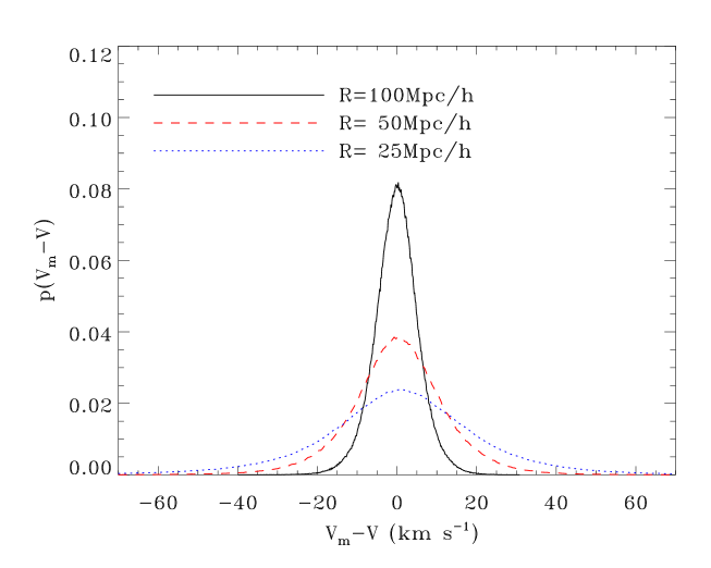
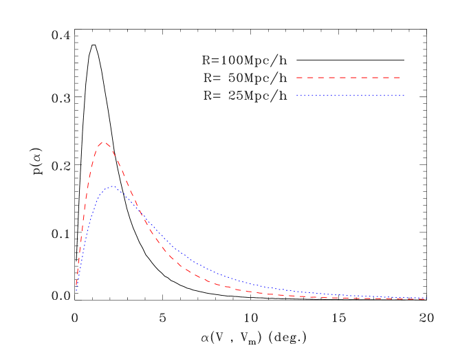
Figure 3.— Differences between $\mathbf{V}$ and $\mathbf{V_{m}}$ in simulation. $R$ is the radius of the spherical top-hat window function. Left: the relative difference between $p(V_{m})$ and $p(V)$, the large fluctuation at the large $V$ is due to the almost zero values of PDFs at tail. Middle: PDFs of amplitude difference between $\mathbf{V}$ and $\mathbf{V}_{m}$ in the same cell. Right: distribution functions of the angle between $\mathbf{V}$ and $\mathbf{V}_{m}$ in the same cell, $\alpha=\cos^{-1}[\mathbf{V}\cdot\mathbf{V}_{m}/(VV_{m})]$.

It is known that attenuation to CMB temperature resulted from kSZ effect $\Delta T_{kSZ}\propto\mathbf{v}\cdot\hat{\mathbf{l}}\int n_{e}{\rm d}l$ in which $\hat{\mathbf{l}}$ is the unit vector of the line-of-sight and $n_{e}$ is the density of free electrons in the galaxy cluster. If the aperture used to measure kSZ effect is sufficiently large, and the number of hot electrons in the cluster can be taken for granted proportional to the mass of host halo $m_{h}$, the total kSZ effect induced temperature fluctuation will be proportional to $m_{h}\mathbf{v}\cdot\hat{\mathbf{l}}$, thus the bulk flow estimated via kSZ effect of galaxy clusters in fact is in principle the mass weighted average of halo velocities,

$$\mathbf{V}_{m}=\frac{\sum_{i}m_{i}\mathbf{v}_{i}}{\sum_{i}m_{i}}\ .$$ (12)

$\mathbf{V}_{m}$ is ratio of two Gaussian random variables, the total mass $M=\sum_{i}m_{i}$ and momentum ${\mathbf{P}}=\sum m_{i}{\mathbf{v}_{i}}$, with the results of Pham-Gia et al. (2006) it is possible to work out a linear theoretical model for $p(V_{m})$. Exact calculation needs knowledge of power spectra of matter, momentum and the correlation function between matter and momentum. However a quick inspection could give us a rough profile. In continuous limit $M=\sum_{i}m_{i}$ becomes $\langle M\rangle[1+\delta*W(R)]$, the smoothed density contrast $\delta*W\ll 1$ if $R$ is large enough to enter the linear regime, therefore $\mathbf{V}_{m}\sim\mathbf{P}/\langle M\rangle$. It has been found that the variance of $\mathbf{P}/\langle M\rangle$ is dominated by the $\sigma_{V}^{2}=(2\pi)^{-3}\int P_{\mathbf{v}\mathbf{v}}\widetilde{W}^{2}{\rm d}^{3}k$ if the smoothing scale is sufficiently large (Park & Park, 2006), so we can expect that $p(\mathbf{V}_{m})\sim p(\mathbf{V})$. Our results of simulation data indeed reveal that differences between $p(\mathbf{V}_{m})$ and $p(\mathbf{V})$ are small (Figure 3).

But in an individual cell $\mathbf{V}_{m}$ does differ from $\mathbf{V}$, both in direction and amplitude. As we can see in Figure 3, $p(V_{m}-V)$ has width of several tens ${\rm km}\,{\rm s}^{-1}$ which decreases with larger cell volume. If the sample volume is small, it could appear that $V_{m}$ deviates from $V$ by $\sim 100{\rm km}\,{\rm s}^{-1}$ though the possibility is tiny. We also notice that $V_{m}-V$ does not show apparent trend with $V$ or $V_{m}$. Pointing of mass weighted bulk flow does not coincide with $\mathbf{V}$. The most likely angle between them is around $1-3$ degrees for top-hat window of $R\in(25,100)h^{-1}$Mpc, and becomes smaller for larger volume. Note that the distribution of the difference angle has a rather long tail, for instance if $R=50h^{-1}$Mpc the probability of misalignment greater than $10^{\circ}$ is $\sim 7.3\%$, yet not trivial.

Hitherto only the kSZ measurements can provide estimation of mass-weighted bulk flow, meanwhile mass weighting does not introduce significant statistical differences, which is actually supported by real observation (Lavaux et al., 2012), thus hereafter we will just concentrate on the unweighted bulk flow.

3.5. Halo mass dependence

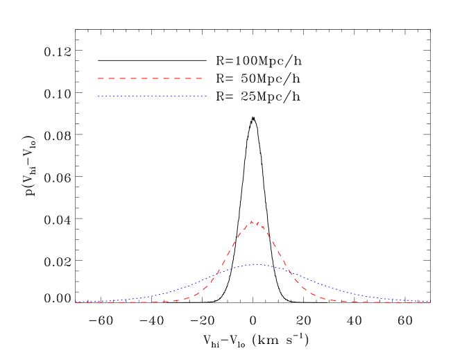
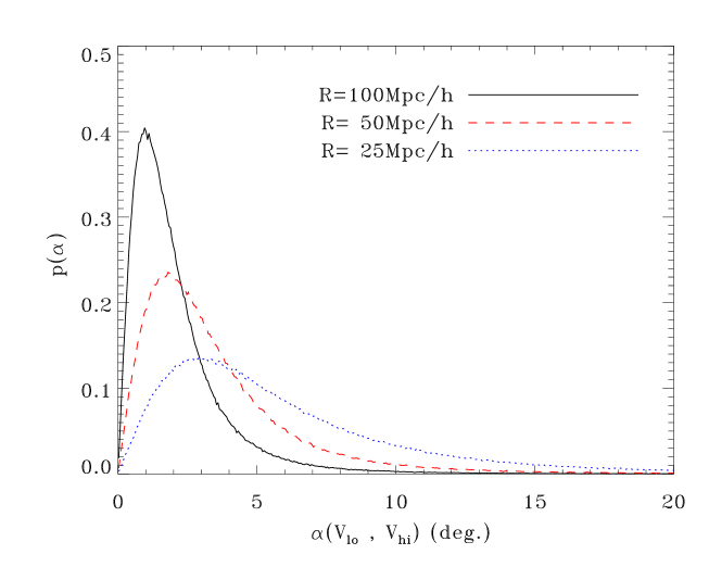
Figure 4.— Halo mass dependence of bulk flow. Left: dependence of $\sigma_{V}$ on halo mass, symbols are measurement, their x-axis coordinates are the mean halo mass of subsamples, lines are prediction of linear theory, below which are labelled with corresponding cell radius. Middle: distribution of amplitude difference between the bulk flow $\mathbf{V}_{lo}$ of the lightest halo subsample ($\bar{m}_{h}=3.015\times 10^{11}h^{-1}M_{\odot}$) and that of the most massive halo subsample $\mathbf{V}_{hi}$ ($\bar{m}_{h}=1.374\times 10^{13}h^{-1}M_{\odot}$) in the same cell. Right: PDFs of the angle between $\mathbf{V}_{lo}$ and $\mathbf{V}_{hi}$, $\alpha=\cos^{-1}[\mathbf{V_{lo}}\cdot\mathbf{V_{hi}}/(V_{lo}V_{hi})]$.

There is the possibility that bulk flow may depends on the typical mass of halo sample. The full halo catalogue is then divided into six subsamples by halo mass, measured $\sigma_{V}$ is plotted in Figure 4 as function of the mean halo mass of the subsample. If the smoothing scale is large it is obvious that there is little dependence on mass of sampled halo of bulk flow. For small sized windows, e.g. $R=25h^{-1}$Mpc, the measured $\sigma_{V}$ of low mass subsample is slightly lower than that of high mass subsample, which might be just statistical fluctuation.

For individual cells, the diversity in bulk flows measured from different halo mass bins might be non-trivial provided that both of $R$ and $V$ are not very large (Figure 4). Considering the fact that intrinsic properties of galaxies and galaxy clusters are more or less correlated with their host halo mass, in case that the sample depth is shallow and estimated bulk flow is of low amplitude, it would not be strange to meet with the difficulty of achieving tight convergence among different samples.

3.6. Consistency between observation and model

Systematical biases in dark flow, the bulk flow measured at high redshift, are not fully understood and precisely controlled, so we refrain ourselves from discussing high redshift case. Most of the local (or nearby) bulk flow measurements has redshift less than $\sim 0.06$, resulting redshift evolution of $\sigma_{V}$ with respect to $z=0$ is of magnitude of a few percents at most, which can be comfortably ignored. Window functions in different works are not the same at all, but the excellent performance of the linear model provides an unified scheme. Since PDFs of bulk flow is solely determined by $\sigma_{V}$, independent of the type of the window, the radius of a top-hat window which gives the same linear $\sigma_{V}$ as the window function used in observation can acts as the effective scale corresponding to a particular sample.

To check if an observed bulk flow is consistent with $\Lambda$CDM model, we need to figure out the variance ranges of $V$. The most likely amplitude of $V$ is $V_{p}=\sqrt{2/3}\sigma_{V}$, derived via ${\rm d}p(V)/{\rm d}V=0$, and the variance range at different levels are computed through Eq. 7. Given significance levels of $1\sigma$, $2\sigma$ and $3\sigma$, corresponding confidence probabilities are $\epsilon_{1,2,3}=68.3\%,95.5\%,99.7\%$ respectively, we choose to define variance range $\Delta V$ of $V$ around $V_{p}$ at specified level through

$$P(|V-V_{p}|\geq\Delta V_{1,2,3})\leq 1-\epsilon_{1,2,3}\ .$$ (13)

Since by definition $V\equiv|\mathbf{V}|\geq 0$ and the probability $\int_{0}^{2V_{p}}p(V){\rm d}V=95.4\%<\epsilon_{2,3}$, to stick with Eq. 13 variance ranges at $2\sigma$ and $3\sigma$ levels shall be translated to $(0,V_{p}+\Delta V_{2,3})$ in that $\int_{0}^{V_{p}+\Delta V_{2,3}}p(V){\rm d}V=\epsilon_{2,3}$, while the $1\sigma$ variance range is the usual one, $(V_{p}-\Delta V_{1},V_{p}+\Delta V_{1})$ with $\int_{V_{p}-\Delta V_{1}}^{V_{p}+\Delta V_{1}}p(V)dV=\epsilon_{1}$. Numerical computation with Eq. 7 then tells that $\Delta V_{1}=0.38875\sigma_{V}$, $\Delta V_{2}=0.81904\sigma_{V}$ and $\Delta V_{3}=1.35577\sigma_{V}$.

Several recent measurements from observational data are over-plotted upon model prediction in Figure 5. One has to keep in mind that our calculation of effective scales has assumed that all other factors affecting estimation have been perfectly corrected, such as non-linearity, selection function and sky coverage incompleteness. Construction details of these samples are often too sketchy to render appropriate weights for our calculation. However the imperfection actually reduces their effective volumes so that the true effective scales will be smaller, i.e. the data points will shift leftward along horizontal axis in Figure 5. So we shall deem Figure 5 as the mostly conservative judgment of the consistency between observation and theory. Nonetheless, from Figure 5, it appears that observation of our local Universe does not rule out the $\Lambda$CDM model. Those results of Haugbølle et al. (2007), Feldman et al. (2010) and Weyant et al. (2011) that often quoted as supporting evidence disfavoring standard $\Lambda$CDM model are around $3\sigma$ level, but the significance will be smaller if error bars are taken into account. In addition, considering that many other measurements (including the not officially published report of Wang, 2007) are in fact consistent with $\Lambda$CDM model, we prefer to choose conservative standpoint on the issue.

Figure 5.— Measured local bulk flows against prediction of linear model. Symbols are some recently estimated amplitudes of local bulk flows from observational data of galaxies (Feldman et al., 2010; Nusser & Davis, 2011) and supernovae (Haugbølle et al., 2007; Colin et al., 2011; Dai et al., 2011; Weyant et al., 2011). Solid line is the model predicted most likely bulk speed, dashed lines indicate variance at $1\sigma$ level ($68.3\%$), dot-dashed line and dotted line are at levels of $2\sigma$ ($95.5\%$) and $3\sigma$ ($99.7\%$) respectively.

3.7. Bulk flow and mass distribution in the cell

It is interesting to investigate the relation between bulk flow and the mass distribution in the sample volume, one might wonder whether one could infer bulk flow from mass distribution if peculiar velocity data is absent, since in linear regime Fourier modes of velocity field can be derived from modes of the density field. However from Eq. 2 it is clear that bulk flow is determined by those modes of wavelengths larger than the characteristic scale of the window function, if the Fourier transformation of the density field is restricted to the same volume in which bulk flow is measured, those modes of long wavelength accounted for bulk flow are missing. In fact it has been clearly shown by Nusser & Davis (1994) that bulk flow is completely immune to internal mass distribution.

Our measurements confirm the expectation. The first quantity we checked is the mass monopole, the total mass ($\sum_{i}m_{i}$) or the total number ($N$) of halos in the volume, which is equivalent to the density fluctuation smoothed by the window function. Correlation coefficients are computed to denote the correlation strength between amplitudes of bulk flow and mass monopole (Table 1). Apparently bulk flow is not correlated with the total mass and the total number of halos in the volume at all.

Two kinds of dipoles of halo distribution are measured, $\langle\mathbf{r}_{i}/r_{i}\rangle$ and the mass weighted one $(\sum m_{i}\mathbf{r}_{i}/r_{i})/\sum m_{i}$. Our results show that including halo mass or not makes little difference. As can be seen in Table 1 and Figure 6, mass dipole correlates with bulk flow very weakly both in amplitude and direction. The correlation becomes slightly tighter as sample volume increases, the peak of the distribution function of the misalignment angle between mass dipole and bulk velocity is at $\sim 45^{\circ}$ for $R=25h^{-1}$Mpc while shifts to $\sim 32^{\circ}$ for $R=100h^{-1}$Mpc (Figure 6).

Table 1Correlation coefficients between amplitude of bulk flow and mass distribution

Cell radius		Mass monopole			Mass dipole
R ($h^{-1}$Mpc   )		$\sum_{i}m_{i}$	$N$		$\frac{\sum m_{i}\mathbf{r}_{i}/r_{i}}{\sum m_{i}}$	$\langle\frac{\mathbf{r}_{i}}{r_{i}}\rangle$
25		0.024	-0.0004	$\ldots$	0.139	0.134
50		0.004	-0.0188	$\ldots$	0.188	0.187
100		0.014	-0.0031	$\ldots$	0.245	0.249

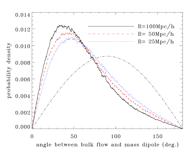
Figure 6.— Probability distribution function of the angle between bulk flow and mass dipole. Dash-dot line is the expectation of null correlation.

4. The fastest bulk flow

There are some works claim detection of unusually large bulk flow (e.g. Feldman et al., 2010; Weyant et al., 2011), it is interesting to check properties of these special parts in $\Lambda$CDM universe. The largest amplitudes of bulk motion measured in our simulation for $R=25,50,100h^{-1}$Mpc are $1070,778,514{\rm km}\,{\rm s}^{-1}$ respectively, the one for $R=100h^{-1}$Mpc is already very close to those observational results. The possibility of residing in the cell having the fastest bulk motion is defined by the ratio of the cell volume to the total volume of simulation, $\approx 0.42\%$ for $R=100h^{-1}$Mpc. However, given the diameter of the cell as large as $200h^{-1}$Mpc against the simulation box length $1h^{-1}$Gpc, a huge volume moving at speed more than $\sim 500{\rm km}\,{\rm s}^{-1}$ will yield observable features too prominent to be missed.

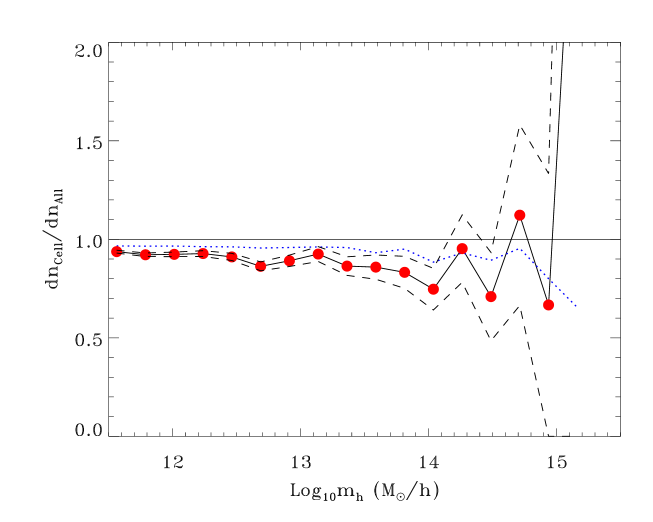
Figure 7.— Difference in halo abundance between the fastest cell with $R=100h^{-1}$Mpc and the full halo catalogue, ${\rm d}n_{Cell}/{\rm d}n_{All}$, ${\rm d}n_{Cell}$ is the mass function of halos in the fastest cell, ${\rm d}n_{All}$ is of the full halo catalogue. Red solid circles connected by solid line is of the fast cell, which is enclosed by dashed lines marking its Poisson variance. The blue dotted line is the average of the top-ten fastest cells. The horizontal solid line is of ${\rm d}n_{Cell}/{\rm d}n_{All}=1$.

In this report we will choose the $R=100h^{-1}$Mpc case as example to study peculiarity of the cell showing fastest bulk motion. The first physical quantity checked is the halo mass function in the cell, for comparison halo mass functions of the top-ten fastest cells (centers separated by at least $100h^{-1}$Mpc) are also measured. Shown in Figure 7 are measured cell halo mass functions divided by the halo abundance in the full catalogue. Among the ten cell mass functions, most (more than 7 of 10) are smaller than the halo mass function of the full catalogue for $m_{h}<\sim 10^{14}h^{-1}M_{\odot}$) In high mass regime due to the very small number of high mass halos we can not withdraw any reliable conclusions though the mass function of the fastest cells demonstrates a high tail. So far we would only cautiously conclude that in high bulk flow regions there is the tendency of finding less number of small mass halos.

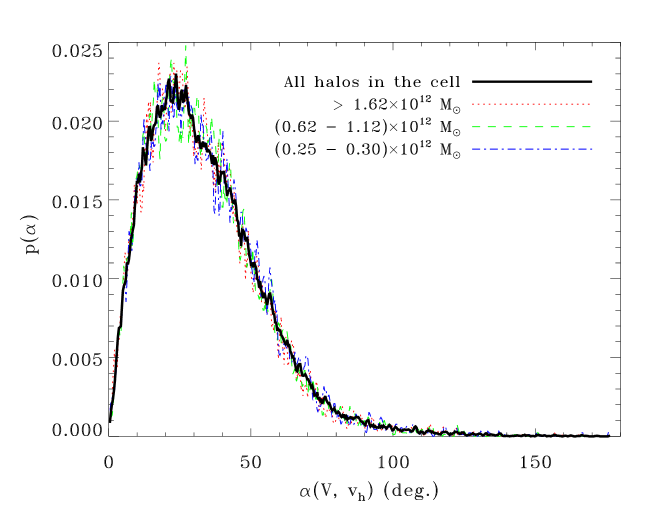
Figure 8.— Velocity distribution of halos in the cell with the largest bulk flow ($R=100h^{-1}Mpc$). Left panel is the distribution of amplitudes of halo velocities, think solid line is of halos in the cell, think solid line is of the full halo catalogue, other color lines are of halos in three different mass bins as labelled in figure legend. Right panel presents distributions of the angle between bulk flow $\mathbf{V}$ and halo velocity $\mathbf{v}_{h}$, $\alpha=\cos^{-1}[\mathbf{V}\cdot\mathbf{v}_{h}/(Vv_{h})]$.

Distribution of all halo velocities in the cell is illustrated in Figure 8, also shown are velocity distribution functions of these halos in mass bins $(0.25-0.3)\times 10^{12}h^{-1}M_{\odot}$, $(0.62-1.12)\times 10^{12}h^{-1}M_{\odot}$ and $>1.62\times 10^{12}h^{-1}M_{\odot}$. Mass binned halos do not exhibit any significant differences in aspect of velocity distribution, which eases the worry of possible bias in mass selected halo samples. Distribution function of the angle between halo velocity and bulk flow is very skewed toward small misalignment, the peak is around $20\sim 30^{\circ}$ but not the $0^{\circ}$, about $90\%$ halos are moving in direction within $60^{\circ}$ to the bulk flow. It appears that halos in the cell with largest bulk velocity are more likely to have higher speed, the peak of velocity amplitude distribution of halos in the cell is at around $600{\rm km}\,{\rm s}^{-1}$ while that of the full halo catalogue is at $\sim 380{\rm km}\,{\rm s}^{-1}$ (Figure 8).

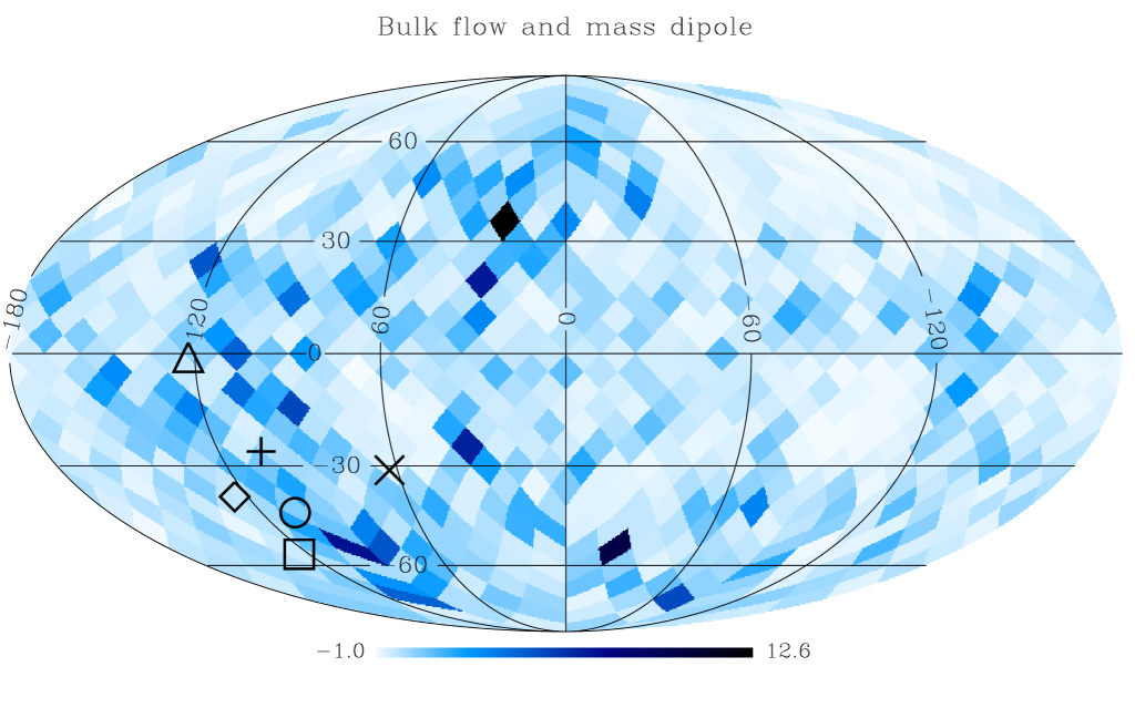
Figure 9.— Mollweide projection of directions of the largest bulk flow and mass dipoles. Mass dipoles are computed from the mass field represented by halos, $\sum m_{i}\mathbf{r}_{i}/r_{i}$. The plus symbol marks the direction of the largest bulk flow ($514{\rm km}\,{\rm s}^{-1}$, cell radius $R=100h^{-1}$Mpc), the cross symbol is the direction of dipole of halos in the cell, the angle between them is $37.4^{\circ}$. Triangle, square, diamond, and circle symbols are directions of mass dipoles within shells $(100,150),(150,200),(200,250),(250,300)h^{-1}$Mpc, which deviate from the bulk flow by about $30^{\circ}$, $33^{\circ}$, $21^{\circ}$, $17^{\circ}$ respectively. The color map is the surface mass density contrast of halos in the cell, plotted in the Healpix scheme (dark color for high density contrast).

It has been examined that bulk flow basically is weakly correlated with the internal mass dipole on average. But for the cell with the largest bulk flow, intuitively one would conjecture there should be certain very massive clumps neighboring to the cell, their gravitational action may play a dominant roll in causing such extreme bulk flow of nearby halos. As an attempt to justify the paradigm, mass dipoles in shells within $R=100-300h^{-1}$Mpc to center of the $100h^{-1}$Mpc cell with largest bulk flow are calculated in four layers with the help of the Healpix package (Górski et al., 2005), if there is unusual distribution of matter in a layer, mass dipole of the layer will be the efficient indicator. Projected directions of bulk flow and mass dipoles are displayed in Figure 9. When shell moves outward mass dipole pointing walks fairly randomly around the bulk flow, the misalignment angle varies between $\sim 20-40^{\circ}$ which is analogous to the typical value in Figure 6. It seems that dipoles of local environmental mass are only aligned crudely with the bulk flow. The correlation is not negligible, however since these misalignment angles are not small, we have no strong support from the simulation to attribute the extremely large bulk flow in such a huge volume mainly to inhomogeneous environment.

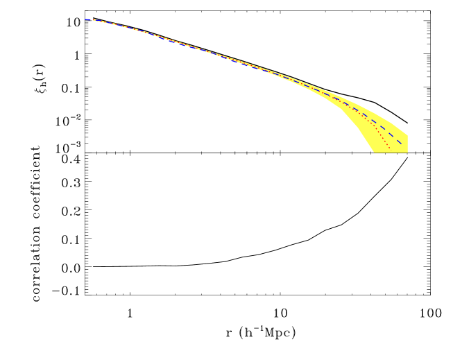
Figure 10.— Correlation between bulk velocity and clustering of halos in the cell, cell radius is $R=100h^{-1}$Mpc. Top panel: solid line is the two-point correlation function $\xi_{h}$ of halos in the cell with the largest bulk velocity, dotted line in red is the average over 1000 $\xi_{h}$s measured in randomly selected cells while the yellow shadow marks the corresponding 1$\sigma$ variance, dashed line in blue is the result of all halos in our halo catalogue. Bottom: correlation coefficients between amplitude of bulk velocity and $\xi_{h}(r)$ as function of $r$, summarized from measurements of 1000 randomly selected cells.

Anomaly in clustering of halos in the special cell is detected (Figure 10), halo two-point correlation functions of 1000 randomly located cells of radius $100h^{-1}$Mpc and the full halo catalogue are also calculated. $\xi_{h}$ averaged over the 1000 measurements agrees with $\xi_{h}$ of the full halo catalogue at scales $r\lesssim 30h^{-1}$Mpc, then drops down more quickly to zero at larger scales due to the integral constraint resulted from finite volume of cell (Landy & Szalay, 1993). As we are interested in $\xi_{h}$ in a finite volume, we did not bother ourselves to apply relevant correction. $\xi_{h}$ of the cell with largest bulk velocity is higher than the average of random cells by around $2\sigma$ at scales $r\lesssim 20h^{-1}$Mpc, at larger scales the excess of clustering power rises to level of $\sim 2-3\sigma$. In order to assess the statistical significance of the event, correlation coefficients of bulk flow amplitude and $\xi_{h}(r)$ are computed from the 1000 random cells (bottom panel in Figure 10). Little correlation is detected at scales $r\lesssim 20h^{-1}$Mpc, then at larger scales the correlation becomes much stronger, indicating that in cells with high bulk velocity it is truly more possible to find power excess in halo clustering at large scales, which appears to be in line with the findings in Macaulay et al. (2011). We further check the halo two-point correlation functions in the top-ten fastest cell, and we find that 7 of the 10 demonstrate power excess at similar scales. Note that the power excess at large scales can not be ascribed to integral constraint, for the leading term of integral constraint in this regime is negative and will bend $\xi_{h}$ downward (Landy & Szalay, 1993).

5. summary and discussion

Through analysis of the Pangu simulation, it is confirmed that bulk flow of halos follows Maxwellian distribution which is completely determined by a single parameter,the bulk velocity dispersion. We find that the dispersion measured in simulation agrees with the prediction of linear perturbation theory of structure formation very well, non-linearity only becomes important when the sampling volume is very small. In most cases mass weighted bulk flow has some minor statistically differences to the unweighted one, but the will not affect the overall statistics significantly. It is also revealed that statistically bulk flow has little systematical dependence on the mass of halos used for estimation. Based on the results, we propose a unified scheme to compare results from observational samples with theories. In the proposal, the scale at which bulk flow in a particular space of the Universe is measured is chosen to be the effective scale $R$ which is the radius of a spherical top-hat window function $W_{th}$ that yields the same bulk velocity dispersion $\sigma_{V}$ as the practical window function $W_{O}$ for the observational sample does in linear theory. $W_{O}$ is not only determined by the sample geometry but also contains weights emerged from selection function, incompleteness and etc., being analogous to the window function used in estimation of power spectrum. Numerical experiments indicate that effects of selection functions on bulk flow estimation could be corrected to a good accuracy by the simple treatment of Eq. 10.

Variance ranges of bulk flow are clarified as well on the basis of Maxwellian distribution in the work, we make a rough comparison of some recently measurements with the $\Lambda$CDM model adopted in Pangu simulation, we find that part results do deviate from the model by about $3\sigma$ but the tension between observation and model is not so strong as original works claimed. Estimated effective scales for observation results in Figure 5 are in fact the upper limits, the true effective scales could be even smaller since we have assumed that those samples are of full sky coverage and their selection functions have been corrected for during estimation. Furthermore, observed bulk velocity consists of residuals from thermal motion of galaxies in their host halo, which is not included in calculation of the velocity dispersion so far. More accurate modeling could be developed by assuming velocities of galaxies relative to their halos obey certain simple distribution, but it requires explicit knowledge of occupation details of galaxies in host halo, which in itself is already a challenging problem. A better way would be to deduct the random motion component in the estimation procedure, such as the treatment in Wang (2007).

Correlation between bulk flow and dipole of internal mass is very weak, but is stronger for larger volume. If one happens to be living in a volume of radius greater than $100h^{-1}$Mpc with large bulk velocity, their observed mass dipole in the volume will have considerable chance of being unusually strong. Typical misalignment angle between bulk flow and mass dipole is mostly likely around $\sim 30-50^{\circ}$. This might introduce non-negligible systematical bias to cosmological probes involving local mass distribution, such as the late-time integrated Sachs-Wolfe effect (Rees & Sciama, 1968).

In our simulation there do exist volume of scale extending to $200h^{-1}$Mpc in diameter moving with extreme large bulk velocity more than $500{\rm km}\,{\rm s}^{-1}$. Most halos inside the volume are moving in alignment with the bulk flow within $60^{\circ}$, and the flow shows no dependence on halo mass. Such group motion of numerous halos will generate prominent kSZ signals, it is a rare event, but given its high speed and huge scale ($200h^{-1}$Mpc versus $1h^{-1}$Gpc), probability of detection is actually not very small, which of course also depends on the inclination between bulk flow and line-of-sight. Another possible observation effect is that galaxies in the volume could be dimmed or brightened on average by the extreme bulk flow than galaxies in other places, which is the starting point of the effort tried by Nusser et al. (2011) and Abate & Feldman (2012).

Dipoles of mass outside the largest bulk flow region as environment are not tightly aligned with the bulk velocity, but deviate from it by around $\sim 20-40^{\circ}$. Interestingly we identified that halo clustering of the particular volume is strengthened apparently at scales $r\gtrsim 20h^{-1}$Mpc, simulation results point out that such enhancement is not completely accidental, at large scales two-point correlation function of halos in a finite volume is indeed mildly correlated with bulk velocity. Bulk velocity is dominated by Fourier modes of velocity at scales larger than the characteristic scale of the sample while in linear theory $\mathbf{v}(\mathbf{k})\propto i\mathbf{k}\delta(\mathbf{k})/k^{2}$, unusually large bulk velocity seems to imply that there should be extraordinary super large mode of density fluctuation topping up in the region. However bulk flow is hardly correlated with the total number or mass of enclosed halos inside the sample volume, and as we checked the total number or mass of halos in the cell with largest bulk velocity is less than the mean value but still within $2\sigma$ variance range. Moreover, in linear regime Fourier modes of density fluctuation are independent, $\xi$ of halos inside the volume is controlled actually by modes of scale less than the characteristic scale of the sample.

Aside from the theoretical puzzle, one question is whether the power excess of halo clustering in a region at scales $\gtrsim 20h^{-1}$Mpc can be used as indicator of candidate space of extremely large bulk flow, the advantage of using two-point correlation function is that clustering does not rely on direction of line-of-sight, the complication resulted from redshift distortion in principle can be overcame by the ratio of $\xi_{h}(r\sim 20-50h^{-1}{\rm Mpc})$ to $\xi_{h}$ at small scales e.g. $\sim 10h^{-1}$Mpc where $\xi_{h}$ is not correlated with bulk flow. A more serious concern is that if we are unluckily (or luckily) in a special region as large as our current largest galaxy survey with extremely large bulk flow, the measured clustering strength at and beyond scale of baryonic acoustic oscillation would be significantly leveled up, could it be the case of power excess at very large scales in the Baryon Oscillation Spectroscopic Survey (BOSS) elaborated by Ross et al. (2012)? To answer all these queries one surely needs multiple realizations of simulation of volume much bigger than our Pangu simulation, for the moment in this paper we have to leave these questions open.

References

- Abate & Feldman (2012) Abate, A., & Feldman, H. A. 2012, MNRAS, 419, 3482
- Afshordi et al. (2009) Afshordi, N., Geshnizjani, G., & Khoury, J. 2009, JCAP, 8, 30
- Amanullah et al. (2010) Amanullah, R., et al. 2010, ApJ, 716, 712
- Bahcall et al. (1994) Bahcall, N. A., Cen, R., & Gramann, M. 1994, ApJ, 430, L13
- Ciecielg & Chodorowski (2004) Ciecielg, P., & Chodorowski, M. J. 2004, MNRAS, 349, 945
- Colin et al. (2011) Colin, J., Mohayaee, R., Sarkar, S., & Shafieloo, A. 2011, MNRAS, 414, 264
- Courtois et al. (2011) Courtois, H. M., Tully, R. B., Makarov, D. I., Mitronova, S., Koribalski, B., Karachentsev, I. D., & Fisher, J. R. 2011, MNRAS, 414, 2005
- Dai et al. (2011) Dai, D.-C., Kinney, W. H., & Stojkovic, D. 2011, JCAP, 4, 15
- Feldman et al. (2010) Feldman, H. A., Watkins, R., & Hudson, M. J. 2010, MNRAS, 407, 2328
- Górski et al. (2005) Górski, K. M., Hivon, E., Banday, A. J., Wandelt, B. D., Hansen, F. K., Reinecke, M., & Bartelmann, M. 2005, ApJ, 622, 759
- Haugbølle et al. (2007) Haugbølle, T., Hannestad, S., Thomsen, B., Fynbo, J., Sollerman, J., & Jha, S. 2007, ApJ, 661, 650
- Jarosik et al. (2011) Jarosik, N., et al. 2011, ApJS, 192, 14
- Jha et al. (2007) Jha, S., Riess, A. G., & Kirshner, R. P. 2007, ApJ, 659, 122
- Kashlinsky et al. (2011) Kashlinsky, A., Atrio-Barandela, F., & Ebeling, H. 2011, ApJ, 732, 1
- Kashlinsky et al. (2010) Kashlinsky, A., Atrio-Barandela, F., Ebeling, H., Edge, A., & Kocevski, D. 2010, ApJ, 712, L81
- Lahav et al. (1991) Lahav, O., Lilje, P. B., Primack, J. R., & Rees, M. J. 1991, MNRAS, 251, 128
- Landy & Szalay (1993) Landy, S. D., & Szalay, A. S. 1993, ApJ, 412, 64
- Lavaux et al. (2012) Lavaux, G., Afshordi, N., & Hudson, M. J. 2012, ArXiv e-prints, astro-ph.CO/1207.1721
- Lewis et al. (2000) Lewis, A., Challinor, A., & Lasenby, A. 2000, ApJ, 538, 473
- Linder (2005) Linder, E. V. 2005, Phys. Rev. D, 72, 043529
- Ma & Scott (2012) Ma, Y.-Z., & Scott, D. 2012, ArXiv e-prints, astro-ph.CO/1208.2028
- Macaulay et al. (2011) Macaulay, E., Feldman, H., Ferreira, P. G., Hudson, M. J., & Watkins, R. 2011, MNRAS, 414, 621
- Mak et al. (2011) Mak, D. S. Y., Pierpaoli, E., & Osborne, S. J. 2011, ApJ, 736, 116
- Mersini-Houghton & Holman (2009) Mersini-Houghton, L., & Holman, R. 2009, JCAP, 2, 6
- Moscardini et al. (1996) Moscardini, L., Branchini, E., Brunozzi, P. T., Borgani, S., Plionis, M., & Coles, P. 1996, MNRAS, 282, 384
- Nusser et al. (2011) Nusser, A., Branchini, E., & Davis, M. 2011, ApJ, 735, 77
- Nusser & Davis (1994) Nusser, A., & Davis, M. 1994, ApJ, 421, L1
- Nusser & Davis (2011) —. 2011, ApJ, 736, 93
- Nusser et al. (1991) Nusser, A., Dekel, A., Bertschinger, E., & Blumenthal, G. R. 1991, ApJ, 379, 6
- Osborne et al. (2011) Osborne, S. J., Mak, D. S. Y., Church, S. E., & Pierpaoli, E. 2011, ApJ, 737, 98
- Park & Park (2006) Park, C.-G., & Park, C. 2006, ApJ, 637, 1
- Pham-Gia et al. (2006) Pham-Gia, T., Turkkan, N., & Marchand, E. 2006, Communications in Statistics - Theory and Methods, 35, 1569
- Rees & Sciama (1968) Rees, M. J., & Sciama, D. W. 1968, Nature, 217, 511
- Ross et al. (2012) Ross, A. J., et al. 2012, MNRAS, 424, 564
- Sandage et al. (2010) Sandage, A., Reindl, B., & Tammann, G. A. 2010, ApJ, 714, 1441
- Saunders et al. (2000) Saunders, W., et al. 2000, MNRAS, 317, 55
- Scoccimarro (2004) Scoccimarro, R. 2004, Phys. Rev. D, 70, 083007
- Song et al. (2011) Song, Y.-S., Sabiu, C. G., Kayo, I., & Nichol, R. C. 2011, JCAP, 5, 20
- Springel (2005) Springel, V. 2005, MNRAS, 364, 1105
- Springob et al. (2007) Springob, C. M., Masters, K. L., Haynes, M. P., Giovanelli, R., & Marinoni, C. 2007, ApJS, 172, 599
- Strauss & Willick (1995) Strauss, M. A., & Willick, J. A. 1995, Phys. Rep., 261, 271
- Sunyaev & Zeldovich (1980) Sunyaev, R. A., & Zeldovich, I. B. 1980, MNRAS, 190, 413
- Szapudi (1998) Szapudi, I. 1998, ApJ, 497, 16
- Turnbull et al. (2012) Turnbull, S. J., Hudson, M. J., Feldman, H. A., Hicken, M., Kirshner, R. P., & Watkins, R. 2012, MNRAS, 420, 447
- Wang (2007) Wang, L. 2007, ArXiv e-prints, astro-ph/0705.0363
- Watkins et al. (2009) Watkins, R., Feldman, H. A., & Hudson, M. J. 2009, MNRAS, 392, 743
- Weyant et al. (2011) Weyant, A., Wood-Vasey, M., Wasserman, L., & Freeman, P. 2011, ApJ, 732, 65
- Wyman & Khoury (2010) Wyman, M., & Khoury, J. 2010, Phys. Rev. D, 82, 044032