Dense Cloud Formation and Star Formation in a Barred Galaxy

Abstract

We investigate the properties of massive, dense clouds formed in a barred galaxy and their possible relation to star formation, performing a two-dimensional hydrodynamical simulation with the gravitational potential obtained from the 2Mass data from the barred spiral galaxy, M83. Since the environment for cloud formation and evolution in the bar region is expected to be different from that in the spiral arm region, barred galaxies are a good target to study the environmental effects on cloud formation and the subsequent star formation. Our simulation uses for an initial 80 Myr an isothermal flow of non-self gravitating gas in the barred potential, then including radiative cooling, heating and self-gravitation of the gas for the next 40 Myr, during which dense clumps are formed. We identify many cold, dense gas clumps for which the mass is more than $10^{4}M_{\odot}$ (a value corresponding to the molecular clouds) and study the physical properties of these clumps. The relation of the velocity dispersion of the identified clump’s internal motion with the clump size is similar to that observed in the molecular clouds of our Galaxy. We find that the virial parameters for clumps in the bar region are larger than that in the spiral arm region. From our numerical results, we estimate star formation in the bar and spiral arm regions by applying the simple model of Krumholz & McKee (2005). The mean relation between star formation rate and gas surface density agrees well with the observed Kennicutt-Schmidt relation. The SFE in the bar region is $\sim$ 60 % of the spiral arm region. This trend is consistent with observations of barred galaxies.

1 Introduction

Star formation (SF) is one of the key processes governing the evolution of galaxies. Many observations of nearby disk galaxies indicate an empirical relation between gas surface density ($\Sigma_{gas}$) and star formation rate surface density ($\Sigma_{SFR}$). This relation is called the Kennicutt-Schmidt (K-S) relation (Schmidt (1959), Kennicutt (1998)). Bigiel et al. (2008) show that $\Sigma_{SFR}$ is well correlated with the hydrogen molecular surface density ($\Sigma_{H_{2}}$) for local spiral galaxies.

Many papers have been devoted to understanding the physical reason behind the K-S relation (e.g. Krumholz & McKee (2005)). However, it remains poorly understood. Since massive stars are mainly observed in the spiral arms of disk galaxies, it has been proposed that star formation is regulated by galactic shocks driven by spiral density waves (e.g. Binney and Tramaine (2008)) and by the increase of cloud-cloud collisions (Tasker & Tan (2009), Tasker (2011)). Krumholz & McKee (2005) propose a star formation model in which star formation efficiency depends on the turbulent properties of the molecular clouds and demonstrate that the Kennicutt-Schmidt relation can be explained by their model. Turbulent internal motion in clouds can be excited by cloud-cloud collisions via the conversion of the orbital energy of the clouds into internal motion energy (Bonnell et al. (2006), Dobbs et al. (2006), Tasker & Tan (2009) and Tasker (2011)).

Barred galaxies show different star formation activity in the bar regions and in the spiral arm regions, even when gas surface density in both regions is comparable (e.g., Downes et al. (1996), Sheth et al. (2000), Muraoka et al. (2007), and Momose et al. (2010)). Studying the physical reason for this discrepancy is an important step to understanding the physics for the K-S relation.

It is well known that the star formation activity is higher in spiral arm regions than in the bar regions, even if the bar regions are gas rich (Momose et al., 2010). We focus on the possibility that this difference is related to a difference in cloud properties between these regions, since the cloud environment is thought to be closely related with SF (Krumholz & McKee (2005)).

Gas flows in the bar regions are elongated with strong shears and dark lanes that are evidence for strong shock waves @( e.g. Wada & Habe (1992)). It is therefore natural to expect clouds forming in this environment to have different properties from elsewhere in the disk.

In this paper, we present a numerical simulation of gas flow at high resolution in a barred galaxy potential. We include cooling and heating processes and study the properties of clouds in different galactic environments within the disk and how this relates to star formation. For the purpose, we resolve gas clumps as small as molecular clouds.

As the first step in our study, we perform a two dimensional simulation with spacial resolution of 4 pc. The galaxy model is that of a barred galaxy with a bar similar to M83. M83 is a nearby barred galaxy, type SABc, and one of the best targets to study the spacial variation of star formation efficiency in a barred galaxy, since it is nearby and has been well observed in various wave lengths, e.g., atomic gas (Huchtmeier & Bohnenstengel, 1981), the molecular gas (Lundgren et al. (2004a), Sakamoto et al. (2004), Muraoka et al. (2007)), optical emission lines (Dopita et al., 2010), X-ray (Soria & Wu, 2003).

From the physical properties of the identified clumps, we estimate the SFE and SFR, using the simple star formation model of turbulent clouds proposed by Krumholz & McKee (2005).

The plan of this paper is as follows: Section 2 describes our model and numerical method. In section 3, we show our numerical results. In section 4, we estimate SFR and SFE in the bar region and the spiral arm region by using the simple model of Krumholz & McKee (2005). In section 5, we present our discussion and conclusion.

2 MODEL and NUMERICAL METHOD

2.1 Model Galaxy

We use a gravitational potential for a barred galaxy similar to that of M83. This model is from the work of Hirota (2009) who analyzed the 2Mass K-band image of M83 (Jarrett et al., 2003), assuming a constant mass to light ratio and a distance of 4.5 Mpc to the galaxy. The model galaxy consists of stellar bulge, stellar bar, stellar disk and dark halo components. The stellar bar end is near $r=2$ kpc from the galactic center and loose spiral arms are traced from the bar end to $r>4.5$ kpc. The circular rotation velocity of the gravitational potential that is shown in Figure 1 roughly agrees with the observation of molecular gas in M83 by Lundgren et al. (2004b). The observed rotation velocity of molecular gas is 150 km/s at 2 kpc from the center and 180 km/s at 3 kpc from the center (Lundgren et al., 2004b). In our simulations, we assume that initial gas rotates in the gravitational potential with a circular velocity that balances the axial averaged gravity of the barred galaxy. The pattern speed of the bar potential is $\Omega_{p}=$ 54 km s^-1 kpc^-1, in keeping with the observed global characteristics of the gas distribution in M83 (Hirota (2009), Hirota et al. (2009)).

For the initial radial distribution of gas mass surface density in the disk, we assume the Gaussian central component and the exponential gas disk component given by Lundgren et al. (2004a) (Fig. 2). The total gas mass within a radius of 6.3 kpc is $3.5\times 10^{9}M_{\odot}$.

2.2 Numerical Method

We simulate two dimensional gas flow in the model galaxy using our M-AUSMPW⁺ code (Namekata & Habe, 2011), which is based on an advection upstream splitting scheme (Kim & Kim, 2005b) with the MLP5 (Kim & Kim, 2005a) for calculating the higher oder numerical fluxes. The size of simulation region is 12.6 kpc $\times$ 12.6 kpc and covers the whole stellar disk of M83. The grid size in our simulation is 3125², with a cell size of 4 pc. We assume as the outer boundary condition of our simulations that physical quantities of hydrodynamics are continuous. We have examined this condition by checking that artificial gas motions are not induced by the outer boundary condition and have found that outward gaseous disturbance in a rotating super sonic gas in the disk galaxy potential propagate without reflection at the outer boundary.

For the first 80 Myrs, we calculate gas motion assuming an isothermal, non self-gravitating gas with $T=10^{4}$K. At this stage, gas density distribution is nearly steady. After this time, we take into account radiative cooling, heating and self-gravity of the gas for the next 40 Myr, which is long enough for the formation of the molecular clouds. Self-gravity of the gas is calculated by FFT of which a detailed description is given in Namekata & Habe (2011). We do not include star formation processes or any stellar feedback throughout our simulation, as we are concentrating on the properties of the clouds formed in the bar galaxy potential. We use a cooling function of gas with a solar metallicity given by Spaans & Norman (1997). For the heating processes, we assume a uniform FUV radiation field and a uniform cosmic ray heating in the energy conservation equation in the numerical hydrodynamics for simplicity. We use the far ultra-violet (FUV) heating rate $\Gamma_{\mathrm{FUV}}=1.0\times 10^{-24}\varepsilon G_{0}$ (Gerritsen and Icke, 1997). We assume $\varepsilon=0.05$ and $G_{0}=1.0$ (Huchtmeier & Bohnenstengel, 1981). These values are obtained in the Galaxy. When radiative cooling is allowed, the gas is allowed to cool to 10 K. For calculation of the cooling rate, gas density is obtained by assuming the thickness of the gas disk is 70 pc.

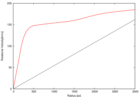
Figure 1: The circular velocity in the model galaxy and the pattern speed of the bar.

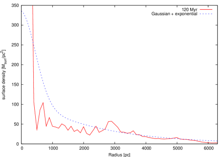
Figure 2: The azimuthally averaged gas surface density at $t=$ 120 Myr (solid line). Dotted line is the initial gas distribution.

2.3 Clump finding method

In order to study the properties of clumps in the bar and spiral arm region, we identify clumps that are dense and have a low temperature by the following method: (A more detailed description is given in Namekata & Habe (2011)). First, cells with a surface density higher than $\Sigma_{\mathrm{cl}}$ and temperature lower than $T_{\mathrm{cl}}$ are selected as a ’candidate’ clump member. Next, if a neighbouring cell to the ’candidate’ is also a candidate, these cells become members of the same group. We iterate this procedure for all candidate cells. If cell number of a group exceeds $n_{\mathrm{cl}}$, the group is identified as a clump.

Since the mean surface gas density is less than $60$M_⊙/pc² except for where $r<500$ pc, as shown in Figure 2, we assume $\Sigma_{\mathrm{cl}}=60$M_⊙/pc² and $n_{\mathrm{cl}}=12$. These values of $\Sigma_{\mathrm{cl}}$ and $n_{\mathrm{cl}}$ correspond to the lower limit mass of clumps of $m_{\mathrm{cl}}\sim 10^{4}M_{\odot}$.

3 RESULTS

3.1 Disk gas evolution

Figure 3 shows the gas surface density distribution at the final stage of the isothermal gas simulation at $t=$ 80 Myr. In this Figure, rotation of the gas and the bar pattern speed are in the counter-clock direction. The major axis of the bar is along the x-axis. Two dominant gas spirals extend from the bar ends and dense gas distributes in the bar region. We continue the simulation with cooling and heating processes and self-gravity of the gas, untill $t=$ 120 Myr.

Figure 4 shows the gas surface density distribution at $t=$ 120 Myr. Many irregular structures of dense gas have formed in the spiral arm and bar regions. In Figure 4, dense gas extends in the bar region more than in Figure 3 and there are many dense gas clumps in the down stream side of the gas flow in the bar region similar to those observed in a barred galaxy. The gaseous bar extends to $r=$2kpc from the center and the loose gaseous spiral arms begin from the gaseous bar ends and extent to $r=$4kpc. These features roughly agree with M83. These dense gas features have a low temperature ($T<100$ K) and are similar to the previous studies (Wada & Norman (2001), Wada & Koda (2001)). From our numerical result as shown in Figure 4 we call a rectangular region ($-2$ kpc $<x<$ 2 kpc and $-1$ kpc$<y<$1 kpc) the bar region and a ring region between $r=2$ kpc and $r=$4 kpc the spiral arm region. There are many dense gas cells with $\Sigma>60M_{\odot}$pc^-2 and $T<100$ K. Total number of the dense gas cells is 341,854 at $t=$ 120 Myr.

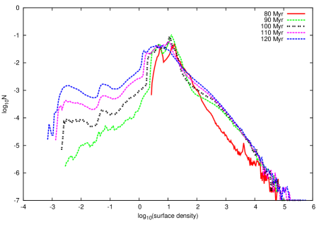
Figure 5: The PDF of surface gas density in unit of $M_{\odot}/$pc${}^{-2}.$ We plot numerical results at $t=80,90,100,110$, and 120 Myr.

We show the probability distribution function (PDF) of surface density in Figure 5. This plot excludes the galactic central region of $r<600$pc where there is a large concentration of gas. The Figure shows that the PDF rapidly changes from $t=$80 Myr to 100 Myr and is almost steady in $t\geq 100$ Myr in the range of $\Sigma>$10 $M_{\odot}$/pc². The PDF in the range of $\Sigma<$1 $M_{\odot}$/pc² appears in $t>80$Myr and is produced by the FUV heating. The FUV heating hardly affects dense part of the PDF in the range of $\Sigma>$10 $M_{\odot}$/pc². The PDF in this stage is approximated by a log-normal form ( Padoan & Nordlund (2002), Wada & Norman (2001)) in the range of $\Sigma>$ 100$M_{\odot}$/pc². The following analysis focusses on the simulation results at $t=120$Myr, since the time between $t=80$ and $t=120$ Myr is long enough to have allowed more than one free-fall time for a typical giant molecular cloud (GMC), e.g. $t_{ff}=\sqrt{3\pi/32G\rho}=4.74(n_{H}/100{\mathrm{c}m}^{-3})^{-0.5}$Myr, and current estimates suggest that GMCs live between 1 and 2 free-fall times (e.g. McKee and Ostriker (2007), and references therin).

We show the radial distribution of the azimuthally averaged gas surface density at $t=$ 120 Myr in Figure 2. There are gas concentrations in the galactic central region ($r<500$pc) and near the bar ends ($r\sim 3$ kpc). These concentrations are formed by gas dynamical effect by the bar potential (e.g., Athanassoula (1992), Wada & Habe (1992)). These characteristic features agree with the observed radial profile of CO ($J=1-0)$ and CO ($J=3-2$) in M83 (Muraoka et al., 2007), except for the large concentration of gas in the central 500 pc region in our numerical result. In M83, there is a nuclear star burst region at the galactic center. The large concentrated gas within 500 pc in our numerical result may be consumed by the nuclear star burst and the discrepancy can be small by the burst star formation.

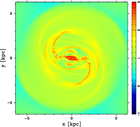
Figure 3: The gas surface density map at $t=$ 80 Myr. Until this stage, gas is isothermal. The color bar in the right hand side shows the logarithmic scale of the surface density of gas in unit of $M_{\odot}$ pc^-2

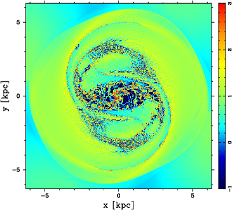
Figure 4: The same as figure 3, but for gas surface density map at $t=$ 120 Myr. Our numerical simulation includes radiative cooling after $t=$ 80Myr.

3.2 Physical properties of the clumps

We select clumps from our numerical results by the method described in section 2.3. These clumps are in the mass range of $10^{4}<M<10^{9}M_{\odot}$. The most massive clump is in $r<100$ pc from the galactic center. The total mass of the clumps is 2.0 $\times 10^{9}M_{\odot}$ in the gas disk. The mass of the clumps in the bar region is 1.3$\times 10^{9}M_{\odot}$ and in the spiral arm region is 0.7 $\times 10^{9}M_{\odot}$. The total number of clumps in the gas disk is 4122. The number of the clumps in the bar region is 495 and in the spiral arm region is 3771.

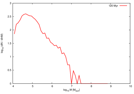
Figure 6: The clump mass function at $t=$ 120 Myr.

We show a mass function of clumps in our numerical result at $t=120$Myr in Figure 6. In this Figure, we plot the number of clumps with an equal spacing of $d\log_{10}M=0.05$. From Figure 6, $dN/dM\propto M^{-1.75}$ in $M>10^{5}M_{\odot}$, since

$${dN\over dM}={1\over M}{dN\over d\ln M}.$$ (1)

This power index agrees well with the observed values $\sim-1.5$ in $M>10^{5}M_{\odot}$ in our Galaxy (Solomon et al., 1987). We test different thresholds of surface density for the clump finding method, and confirm that the power index of the clump mass function is almost independent from the choice of the threshold value.

We plot clump mass vs. their size in Figure 7. Plus symbols show clumps in the bar region. We use the color contour map to show clumps in the spiral arm region which are too numerous to represent as points. The color bar shows number of clumps in the cell given by dividing the plot frame into 200 $\times$ 200. Since the clumps have an irregular shape, in this Figure, we estimate clump size $l$ as:

$$l=(({S\over pc^{2}})/\pi)^{0.5}pc,$$

where $S$ is area of the clump. From Figure 7, we find the relation

$$M_{cl}=10^{4.5}~{}(l/10pc)^{2.5}M_{\odot},$$ (2)

that is shown by a dashed line in Figure 7. Large size clumps of $l>40$ pc are in the bar region and in the galactic central region ($r<500$ pc).

In Figure 8, we plot the one dimensional velocity dispersion, $\sigma_{v}$, of the internal velocity of the clumps vs. their sizes. $\sigma_{v}$ is given by:

$$\sigma_{v}=\sqrt{\frac{1}{2M_{\mathrm{cl}}}\left(\sum_{i,j}\{m_{\mathrm{cl}~{}i,j}({\mn@boldsymbol{v}_{i,j}}-\overline{{\mn@boldsymbol{v}_{\mathrm{cl}}}})^{2}\}\right)}$$ (3)

from our numerical result, where $m_{\mathrm{cl}~{}i,j}$ and $\mn@boldsymbol{v}_{i,j}$ are the gas mass and the velocity of gas in the $(i,j)$ cell belonging to this clump of which mass is $M_{\mathrm{cl}}$, respectively. $\mn@boldsymbol{v}_{cl}$ is velocity of the center of mass of this clump. Relation of the velocity dispersions and sizes of clumps is approximated as

$$\sigma_{v}=0.8~{}(l/1pc)^{0.5}km/s$$ (4)

in the spiral arm region, which is shown by a dashed line in Figure 8. This relation is similar to the results of Larson (1981) and Solomon et al. (1987). Larson (1981) gives $\sigma_{v}=1.1~{}(l/1pc)^{0.38}$ km/s and Solomon et al. (1987) gives $\sigma_{v}=1.0\pm 0.1~{}(l/1pc)^{0.5\pm 0.05}$ km/s. Figure 8 clearly show that there are clumps with larger velocity dispersions in the bar region than in the spiral arm region. The @large velocity dispersion of clumps in the bar region may be due to their formation process; that is, clumps form from cooled gas in gas flow with strong shear motion in the bar region and/or turbulent internal motion in clouds is excited by cloud collisions.

We plot internal velocity dispersion vs. mass of clumps in Figure 9. The relation between the internal velocity dispersion and the mass of clump is approximated as

$$\sigma_{v}=2~{}(M_{cl}/10^{5}M_{\odot})^{0.4-0.5}km/s.$$ (5)

The virial parameter is a useful measure of the gravitational stability of the clumps. Virial parameter of a spherical clump is given by

$$\alpha_{vir}={{5\sigma_{v}^{2}l}\over GM_{\mathrm{MC}}},$$ (6)

where $M_{\mathrm{MC}}$ is its mass, $\sigma_{v}$ is its one dimensional velocity dispersion of internal motion, and $l$ is its size. We modify $\alpha_{vir}$ as

$$\alpha_{vir}={{10\sigma_{v}^{2}l}\over 3GM_{\mathrm{GMC}}},$$

since our numerical calculation is two-dimensional. In Figure 10, we plot the virial parameter $\alpha_{vir}$ vs. mass of clumps. Several clumps in the bar region have larger virial parameters than in the spiral arm region. Number of clumps with $\alpha_{vir}>1$ is 476 of the total 495 clumps in the bar and 2855 of the total 3771 clumps in the spiral arm region. These gravitationally unbound clumps would be transient, since $\alpha_{vir}>1$. Such transient clumps are found in the numerical simulation of giant molecular clouds formation by spiral shocks (Dobbs et al., 2006). In Dobbs et al. (2006), they show that a large part of the formed clouds are gravitational unbound and transient. @ @ Mass fraction of clumps with $\alpha_{vir}<1$ is 4.28 % of the total mass of clumps in the disk, 0.33% of the total mass of clumps is in the bar region and 3.95% of the total mass of clumps is in the spiral arm region. Fraction of clumps with $\alpha_{vir}<1$ is much smaller in the bar than that in the spiral arm region. Small fraction of gravitational unstable clumps in the bar region may be related with low star formation efficiency in the bar region. We will discuss this possibility in section 4.

We plot galactic radial distributions of velocity dispersion of clumps in Figure 11 and virial parameters of clumps in Figure 12. There are more clumps with large virial parameters in $r<2.5$ kpc than that in $r>2.5$ kpc. There are many clumps with $\alpha<1$ in the spiral arm region. From these results, we expect many star forming clumps in the region. In Figure 12, there are small excess of number of clumps with $\alpha<1$ in $r=1.5-2$kpc. The excess is near the bar end where gas orbits are expected to be crowded (Wada & Habe, 1992). The orbit crowding will lead to increase cloud collisions near the bar end. The increase of cloud collisions can explain the excess of clumps with $\alpha<1$, if cloud collisions are inelastic and reduce internal irregular motion in clumps.

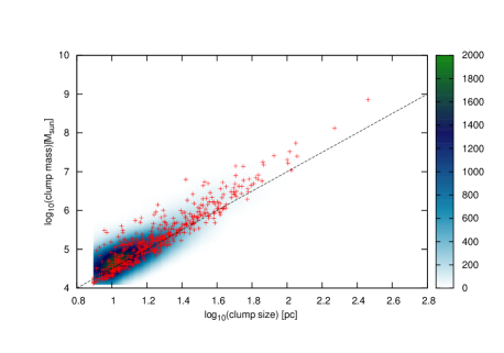
Figure 7: Clump mass vs. clump size for the clumps in our numerical results at $t=$ 120 Myr. Plus symbols show clumps in the bar region and the color contour map shows clumps in the spiral arm region. The color bar shows number of clumps in the cell given by dividing the plot flame into 200 $\times$ 200.

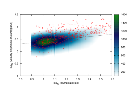
Figure 8: The same as Figure 7, but for the distribution of velocity dispersion of internal motion vs. clump size for the clumps in our numerical results at $t=$ 100 Myr. The dashed line shows the relation given by Solomon et al. (1987)

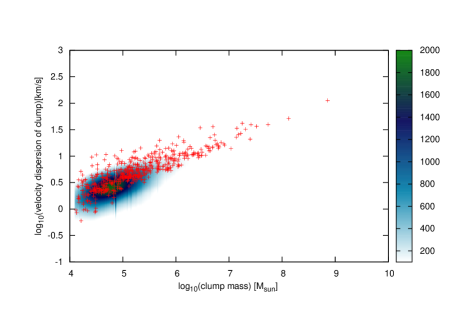
Figure 9: The same as Figure 7, but for the distribution of velocity dispersion of internal motion vs. clump mass for the clumps in our numerical results at $t=$ 120 Myr.

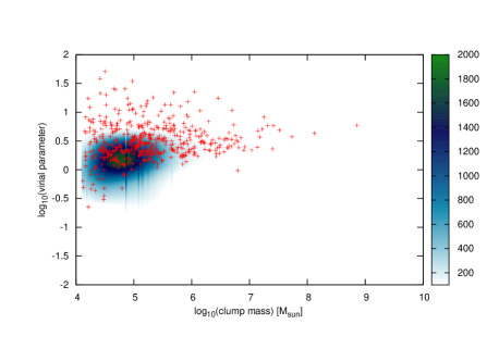
Figure 10: The same as Figure 7, but for the distribution of the virial parameter of clumps with clump mass at $t=$ 120 Myr.

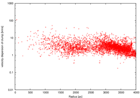
Figure 11: The radial distribution of velocity dispersion of clumps in the galaxy at $t=$ 120 Myr.

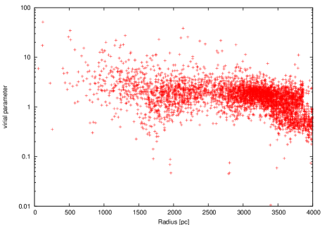
Figure 12: The radial distribution of virial parameter of clumps in the galaxy at $t=$ 120 Myr.

4 Star formation

We estimate the star formation rate from our numerical results. Since the cell size of our numerical simulation, 4 pc, is not enough to resolve the star formation process by hydrodynamical simulation, we use the star formation model proposed by Krumholz & McKee (2005) as sub-grid physics. In their model, they assume that star formation occurs in Jeans unstable parts of the giant molecular clouds and is regulated by the turbulent motions in the giant molecular clouds. In their model, they assume that turbulent velocities in the giant molecular clouds is described by a power law of the size of the turbulent motion, a probability density function for the density is a log normal type and star formation occurs in the Jeans unstable part of the giant molecular cloud. They obtain a star formation rate for a giant molecular cloud as:

$$SFR=SFR_{\mathrm{ff}}{M_{\mathrm{GMC}}\over t_{\mathrm{ff}}}$$ (7)

where

$$t_{ff}=\sqrt{{3\pi\over 32G\rho}}=1.5\left({n_{H}\over 1000\mathrm{cm}^{-3}}\right)^{-1/2}\mathrm{Myr}.$$ (8)

and

$$\mathrm{SFR_{\mathrm{ff}}}=0.014\left(\frac{\alpha_{\mathrm{vir}}}{1.3}\right)^{-0.68}\left(\frac{\mathcal{M}}{100}\right)^{-0.32},$$ (9)

where $\mathcal{M}=\sigma_{v}/c_{s}$ and $c_{\mathrm{s}}$ is the sound speed of clouds. We estimate star formation rate in a clump as

$$\mathrm{SFR}=\left(\frac{\mathrm{SFR_{\mathrm{ff}}}f_{\mathrm{MC}}M_{\mathrm{cl}}}{t_{\mathrm{dyn}}}\right),$$ (10)

where $M_{\mathrm{cl}}$ is the clump mass, $f_{\mathrm{MC}}$ is the fraction of molecular gas of it, and $t_{\mathrm{dyn}}$ is given by

$$t_{\mathrm{dyn}}=\frac{\sigma_{v}}{\pi G\overline{\Sigma}_{\mathrm{cl}}}=1.36\left({\sigma_{v}\over\mathrm{1km~{}s}^{-1}}\right)\left({\overline{\Sigma}_{\mathrm{cl}}\over 50M_{\odot}\mathrm{pc}^{-2}}\right)^{-1}\mathrm{Myr}.$$ (11)

$\overline{\Sigma}_{cl}$ is the mean surface density of each clump. We also calculate ${\mathrm{SFR}}$, assuming ${\mathrm{SFR}}_{ff}=0.014$ for comparison.

4.1 Relation of Star Formation Rate Surface Density and Gas Surface Density

We obtain a SFR from our numerical results by assuming that the SFR for each clump @is given by equation (10) with $f_{\mathrm{MC}}=1$, that is, the clumps are assumed to be mainly composed of H₂ molecules. We show the SFR surface density vs. surface density of mass of clumps over the average scale of 500 pc in Figure 13 (the spiral arm region) and in Figure 14 (the bar region). Figure 13 (a) and Figure 14 (a) show the SFR surface density for the star formation model with SFR_ff of equation (9) as proposed by Krumholz & McKee (2005). These panels show that SFR surface density is lower in the bar region than in the spiral arm region for the same clump mass surface density. This result well corresponds to the obervational results by Momose et al. (2010). For the constant SFR_ff model as shown in Figure 13 (b) and Figure 14 (b), the SFR surface density has smaller scatter than the result by the model of Krumholz & McKee (2005) in both regions and difference of the SFR surface density between these regions is small. This result means that the difference of SFR between the bar and spiral arm regions is mainly due to difference of internal motion of clumps, if the star formation model of Krumholz & McKee (2005) can be applied. Correlation shown in Figure 13 and Figure 14 are well within the relation given by Kennicutt (1998) and Bigiel et al. (2008).

4.2 Radial Distribution of Star Formation Rate

We show the radial distribution of the mean SFR surface density in Figure 15. In Figure 15, we exclude the central region of $r<$ 500 pc, since there is high mass concentration of clumps and the SFR is very high in this region. The SFR between $0.5$ kpc$~{}<r<2.5$ kpc is $\Sigma_{\mathrm{SFR}}\sim 10^{-7.2}M_{\odot}/pc^{2}/yr$ which is smaller than $\sim 10^{-7}M_{\odot}/pc^{2}/yr$ in the region of 2.5 kpc$~{}<r<$3.5 kpc. There are @small enhancements of the SFR near $r=$2 kpc and $r=$3 kpc. The former is near the outer edge of the bar region, and the latter is near the inner ends of gas spirals and corresponds to small number excess of clumps with $\alpha<1$ as shown in section 3. The SFR agrees with the estimation of Muraoka et al. (2007) within their uncertainty as shown in Figure 15.

We show the radial distribution of star formation efficiency (SFE), i.e., star formation rate per unit clump mass, in Figure 16. In this Figure, we also exclude the central region of $r<$ 500 pc. The SFE agrees with the estimation of Muraoka et al. (2007) within their uncertainty as shown in Figure 16. The SFE in the bar region is $\sim 60$ % of the spiral arm region. This trend is observed in barred galaxies ( Muraoka et al. (2007), Momose et al. (2010)). Our numerical results show that many more clumps in the bar region have large virial parameters with $\alpha>1$ than in the spiral arm region. This is the reason why the SFE is small in the bar region. In NGC 4303, SFE is larger than our numerical results with $\sim 10^{-8.5}$ yr^-1 in the bar region and $\sim 10^{-8.5}-10^{-7.5}$ yr^-1 in the spiral arm region. This is because SFR is slightly higher in NGC 4303 than the mean value of the KS relation (Momose et al., 2010).

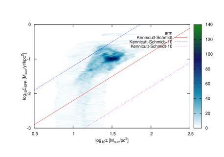
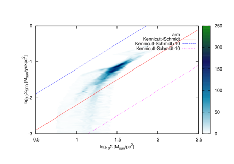
Figure 13: The distribution of the SFR surface density averaged in the scale of 500 pc with the clump mass surface density averaged in the same scale at $t=$ 120 Myr in the spiral arm region for SFR_ff of eq. (9) (top), and for SFR${}_{ff}=0.014$ (bottom). The color bar shows number of cells of numerical hydrodynamic simulation. The red solid line shows the Kennicutt - Schmidt relation. The blue dotted line shows 10 times the Kennicutt - Schmidt relation. The magenta dotted line shows 1/10 the Kennicutt - Schmidt relation.

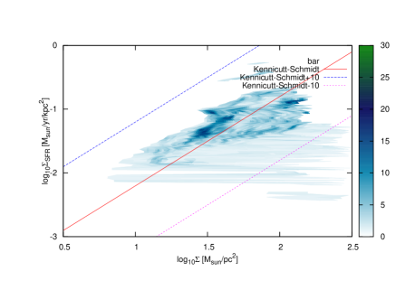
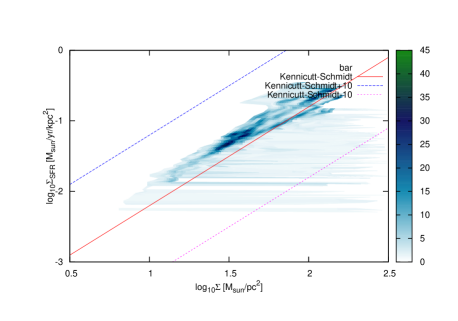
Figure 14: The same as in figure 13, but for the bar regions.

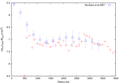
Figure 15: The radial distribution of star formation rate obtained by using the Kulmholts-McKee star formation model in the model galaxy . We show the star formation rate in $r\geq$ 600 pc. We also plot the star formation rate estimated by Muraoka et al. (2007).

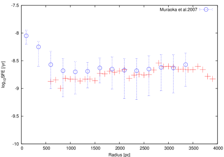
Figure 16: The radial distribution of star formation efficiency in $r>600$pc..

5 DISCUSSION and CONCLUSION

Our numerical results have shown that most of massive clumps in the bar region have large virial parameters, $\alpha$ and that mass fraction of bound clumps in the bar region is smaller than in the spiral arm region, although the mean surface gas density is larger in the bar region than in the spiral arm region as shown in section 3. Lundgren et al. (2004b) shows that molecular gas velocity dispersion is large in the bar region in M83. Sorai et al. (2012) shows that molecular gas in the bar has also large velocity dispersion in a barred galaxy, Maffei 2. Because of large shear gas flow in the bar region, most of clumps formed from gas in the bar region may have large internal gas motions. If cloud collisions in the bar region are more frequent than in the spiral arm region, large internal motion in clouds is also possible to be excited by cloud collisions. These may be the reason why the mass fraction of bound clumps in the bar region is smaller than in the spiral arm region. It is interesting to study these possibility.

The SFR estimation from our numerical results agrees with the K-S relation as shown in section 4. In this analysis, we use the star formation model of Krumholz & McKee (2005) in which they assume that gravitationally unstable parts of the molecular clouds with small turbulent velocities form stars. In their model, they assume the scaling relation between turbulent velocities and turbulent sizes as in Larson (1981). In their model, SF rate is given by the gravitational unstable part mass divided by its free fall time. In our analysis, turbulent velocities of clump sizes are assumed to be the velocity dispersions of internal motions of clumps in our numerical results, @ and equations (10) and (11) are used. We have shown that the SFR surface density is smaller in the bar region than in the spiral arm region for the same gas surface density using the star formation model of Krumholz & McKee (2005). We have also shown that the difference between the bar region and the spiral region is small for the constant SFR_ff model. From these comparison, the difference of SFR surface density can be explained by the difference of internal motions of clumps between these region.

We have examined the radial distributions of SFR and SFE, since our estimation of SFR agrees with the observed Kennicutt-Schmidt relation. Both radial distributions are within the error bars of observation of M83 (Muraoka et al., 2007) in $r>$ 500pc, with the SFR and SFE being smaller in the bar region than in the spiral arm region. The decrease of both SFR and SFE in the bar region is similar to the recent observations of barred galaxies (Momose et al., 2010).

Our numerical results show that the turbulent star formation model can explain the property of star formation in barred galaxies. It is interesting to study observationally the difference in cloud properties in the bar and in the spiral arm regions and the relation between cloud property and SF activity in various environments in galaxies using radio telescopes with high spatial resolution, e.g. ALMA, that will make it possible to resolve molecular clouds in extragalaxies.

We discuss limitations of our numerical simulation. We assume the constant FUV background heating as described in section 2. Our FUV heating rate that corresponds to our Galaxy value has small effect on cold dense gas, as shown in section 3. The assumption of the constant FUV background heating is too simple. Thilker et al. (2005) shows the radial profile of the surface brightnesses in the FUV and NUV bands in M83. The FUV surface brightness is roughly constant from $r=$ 600 pc to $r=$ 2 kpc, has a peak near $r=$2.6 kpc ( $\sim$2 arcminits ), and decreases with radius in $r>2.6$ kpc. This profile indicates that FUV background heating is stronger in the bar region ($r<2.6$ kpc) than in the arm region. If FUV heating is effective to destroy molecular clouds, SFR in the bar region will be reduced. In this case, the decrease of SFR in the bar region in M83 can be explained even without the turbulent SF model given by using equation (9). However, It is not obvious that the observed FUV brightness in M83 is strong enough to suppress SFR in the bar region. We do not consider radial-dependent FUV background heating in this paper. This will be considered in further work. In our simulation, we do not consider feedback from star formation. Feedback by energy released from supernovae and stellar winds can destroy nearby molecular clouds. Strong UV photons from newly formed stars will ionize nearby clouds and the ionization will suppress SF in them. Strong stellar winds and supernova remnants will compress molecular clouds. By the compression, star formation can be triggered. Feedback process is very complicated. If suppression of star formation by feedback is large, difference of SF property between the bar region and the spiral arm region can be reduced. It is very interesting to study how feedback affects molecular cloud property and SF process. In order to consider feedback process, 3D numerical simulations with high resolution are essential, since the destruction process of molecular clouds and expansion of gas by heating of newly formed stars and supernovae are three dimensional phenomena ( e.g. Tasker & Bryan (2006)). We will study feedback effects in barred galaxies by three dimensional simulations in our forth coming papers.

6 ACKNOWLEGMENTS

We acknowledge Elizabeth Tasker for useful comments that helped to improve this paper. We acknowledge the anonymous referee who gives nice comments to improve this paper. We also acknowledge useful discussions with Masayuki Fujimoto, Tetsuhiro Minamidani, Naomasa Nakai, Junya Ito, Junichiro Enomoto and Takashi Ito. Numerical computations were carried out on Cray XT4 at Center for Computational Astrophysics, CfCA, of National Astronomical Observatory of Japan. This work was supported by a Grant-in-Aid for Specially Promoted Research 20001003 (AH).

References

- Athanassoula (1992) Athanassoula, E., 1992, MNRAS. 259, 345
- Bigiel et al. (2008) Bigiel, F., Leroy, A., Walter, F., Brinks, E., de Blok, W. J. G., Madore, B., Thornley, M. D. 2008, AJ. 136, 28
- Binney and Tramaine (2008) Binney, J. and Tremaine, S., Galactic Dynamics, second Ed., Princeton Series in Astrophysics, 2008
- Bolatto et al. (2008) Bolatto, A. D., Leroy, A. K., Rosolowsky, E., Walter, F., Blitz, L. 2008, ApJ. 686, 948
- Bonnell et al. (2006) Bonnell, I. A., Dobbs, C. L., Robitaille, T. P., Pringle, J. E., 2006, MNRAS, 365, 37
- David et al. (2005) David A. et al. 2005, ApJ. 619, L79
- Dobbs et al. (2006) Dobbs, C. L., Bonnell, I. A., Pringle, J. E. 2006, MNRAS. 371, 1663
- Dopita et al. (2010) Dopita, M. A., Blair, William P., Long, K. S., Mutchler, M., Whitmore, B. C., Kuntz, K. D., Balick, B., Bond, H. E., Calzetti, D., Carollo, M., and 16 coauthors 2010, ApJ. 710, 964
- Downes et al. (1996) Downes, D., Reynaud, D., Solomon, P. M., Radford, S. J. E. 1996, ApJ. 461, 186
- Fujimoto (1968) Fujimoto, M. 1968, ApJ. 152, 391
- Gerritsen and Icke (1997) Gerritsen, J. P. E., Icke, V. 1997, A&Ap. 325, 972
- Gnedin et al. (2009) Gnedin, N. Y., Tassis, K., Kravtsov, A. V. 2009, ApJ., 697, 55
- Habing (1968) Habing, H. 1968, Bull. Astron. Inst. Neth., 19, 421
- Handa et al. (1991) Handa T., Sofue Y., Nakai N., 1991, IAUS, 146, 156
- Heyer et al. (2009) Heyer, M., Krawczyk, C., Duval, J., Jackson, J. M. 2009, ApJ. 699, 1092
- Hirota (2009) Hirota, 2009 Private communication.
- Hirota et al. (2009) Hirota, A., Kuno, N., Sato, N., Nakanishi, H., Tosaki, T., Matsui, H., Habe, A., Sorai, K., 2009, PASJ, 61, 441
- Huchtmeier & Bohnenstengel (1981) Huchtmeier, W. K., Bohnenstengel, H.-D. 1981, A&Ap. 100, 72
- Jarrett et al. (2003) Jarrett, T. H., Chester, T., Cutri, R., Schneider, S. E., & Huchra, J. P. 2003, AJ, 125, 525
- Kennicutt (1998) Kennicutt,R.C.Jr. 1998, ApJ, 498, 541
- Kim & Kim (2005b) Kim K. H., Kim C., 2005a, Journal of Computational Physics, 208, 527
- Kim & Kim (2005a) Kim K. H., Kim C., 2005b, Journal of Computational Physics, 208, 570
- Krumholz & McKee (2005) Krumholz M. R., McKee C. F., 2005, ApJ, 630, 250
- Larson (1981) Larson, R. B., 1981, MNRAS,194, 809.
- Lundgren et al. (2004a) Lundgren A. A., Wiklind T., Olofsson H., and Rydbeck G., 2004a, A&A, 413, 505
- Lundgren et al. (2004b) Lundgren, A. A., Olofsson, H., Wiklind, T., Rydbeck, G. 2004b, A& A, 422, 865
- McKee and Ostriker (2007) Mckee,C.F. and Ostriker,E.C., ARA&A, 45, 565.
- Momose et al. (2010) Momose, R., Okumura, S. K., Koda, J., Sawada, T. 2010, ApJ. 721, 383
- Muraoka et al. (2007) Muraoka, K., Kohno, K., Tosaki, T., Kuno, N., Nakanishi, K., Sorai, K., Okuda, T., Sakamoto, S., Endo, A., Hatsukade, B., and 7 coauthors, 2007, PASJ. 59, 43.
- Muraoka et al. (2009) Muraoka, K., Kohno, K., Tosaki, T., Kuno, N., Nakanishi, K., Sorai, K., Sawada, T., Tanaka, K., Handa, T., Fukuhara, M., and 2 coauthors, 2009, ApJ. 706, 1213.
- Namekata & Habe (2011) Namekata D. & Habe A., 2011, ApJ, 731, 57.
- Padoan & Nordlund (2002) Padoan, P. & Nordlund, A. , 2002, ApJ. 576, 870
- Ostriker et al. (2010) Ostriker, E. C., McKee, C. F., Leroy, A. K., 2010, ApJ. 721, 975
- Rosolowsky (2007) Rosolowsky, E. 2007, ApJ. 654, 240
- Sakamoto et al. (2004) Sakamoto, K., Matsushita, S., Peck, A. B., Wiedner, M. C., Iono, D., 2004, ApJ. 616, L59
- Schmidt (1959) Schmidt, M., 1959, ApJ., 129, 243.
- Sheth et al. (2000) Sheth, K., Regan, M. W., Vogel, S. N., Teuben, P. J. 2000, ApJ. 532, 221
- Soria & Wu (2003) Soria, R., Wu, K. 2003, A&Ap. 410, 53
- Spaans & Norman (1997) Spaans M., Norman C. A., 1997, ApJ, 483, 87
- Solomon et al. (1987) Solomon, P. M., Rivolo, A. R., Barrett, J., & Yahil, A., 1987, ApJ, 319, 730
- Sorai et al. (2012) Sorai,K., Kuno,N., Nishiyama,K. Watanabe,Y., Matsui,H. Habe,A., Hirota,A., Ishihara,Y. and Nakai,N. 2012 PASJ, 64, 51
- Tasker (2011) Tasker, E. J., 2011ApJ. 730, 11
- Tasker & Bryan (2006) Tasker, E. J., Bryan, G. L., 2006, ApJ. 641, 878
- Tasker & Tan (2009) Tasker, E. J., Tan, J. C., 2009, ApJ., 700, 358
- Thilker et al. (2005) Thilker, D. A. et al. 2005, ApJ., 619, L79
- Wada & Habe (1992) Wada, K., Habe, A., 1992, MNRAS. 258, 82
- Wada & Koda (2001) Wada, Keiichi, Koda, Jin, 2001, PASJ, 53, 1163
- Wada & Norman (2001) Wada, Keiichi, & Norman, Colin A., 2001, ApJ, 547, 172