An Exploration of the Singularities in General Relativity

Abstract.

In General Relativity, spacetime singularities raise a number of problems, both mathematical and physical.

One can identify a class of singularities – with smooth but degenerate metric – which, under a set of conditions, allow us to define proper geometric invariants, and to write field equations, including equations which are equivalent to Einstein’s at non-singular points, but remain well-defined and smooth at singularities. This class of singularities is large enough to contain isotropic singularities, warped-product singularities, including the Friedmann-Lemaître-Robertson-Walker singularities, etc.Also a Big-Bang singularity of this type automatically satisfies Penrose’s Weyl curvature hypothesis.

The Schwarzschild, Reissner-Nordström, and Kerr-Newman singularities apparently are not of this benign type, but we can pass to coordinates in which they become benign. The charged black hole solutions Reissner-Nordström and Kerr-Newman can be used to model classical charged particles in General Relativity. Their electromagnetic potential and electromagnetic field are analytic in the new coordinates – they have finite values at $r=0$.

There are hints from Quantum Field Theory and Quantum Gravity that a dimensional reduction is required at small scale. A possible explanation is provided by benign singularities, because some of their properties correspond to a reduction of dimensionality.

Seminar held at JINR, Dubna, May 15, 2012.

1. Introduction

1.1. Problems of General Relativity

There are two big problems in General Relativity:

1. It predicts the occurrence of singularities [1, 2, 3, 4, 5].

2. The attempts to quantize gravity seem to fail, because it is perturbatively nonrenormalizable [6, 7].

Are these problems signs that we should give up General Relativity in favor of more radical approaches (superstrings, loop quantum gravity etc.)?

There is another possibility: the limits may be in fact not of GR, but of our tools. Understanding how much we can push the boundaries of GR would be helpful, even in the eventuality that a better theory will replace GR.

1.2. Two types of singularities

There are two types of singularities:

1. Malign singularities: some of the components of the metric are divergent: $g_{ab}\to\infty$.

2. Benign singularities: $g_{ab}$ are smooth and finite, but $\det g\to 0$.

Benign singularities turn out to be, in many cases, manageable [8, 9, 10]. Important malign singularities turn out to be in fact benign, but they appear to be malign because they are represented in singular coordinates [11, 12, 13].

1.3. What is wrong with singularities

If some of metric’s components are divergent (as in the case of malign singularities), everything seems to be wrong. If the metric is smooth, but its determinant $\det g\to 0$, the usual Riemannian invariants blow up. For example, the covariant derivative can’t be defined, because the inverse of the metric, ${\color[rgb]{1,0,0}g^{ab}}$, becomes singular ($g^{ab}\to\infty$ when $\det g\to 0$). This makes the Christoffel’s symbols of the second kind singular:

(1) $$\Gamma^{{\color[rgb]{1,0,0}c}}{}_{ab}=\displaystyle{\frac{1}{2}}{\color[rgb]{1,0,0}g^{cs}}(\partial_{a}g_{bs}+\partial_{b}g_{sa}-\partial_{s}g_{ab})$$

The Riemann curvature is singular too:

(2) $$R^{{\color[rgb]{1,0,0}d}}{}_{abc}=\Gamma^{{\color[rgb]{1,0,0}d}}{}_{ac,b}-\Gamma^{{\color[rgb]{1,0,0}d}}{}_{ab,c}+\Gamma^{{\color[rgb]{1,0,0}d}}{}_{bs}\Gamma^{{\color[rgb]{1,0,0}s}}{}_{ac}-\Gamma^{{\color[rgb]{1,0,0}d}}{}_{cs}\Gamma^{{\color[rgb]{1,0,0}s}}{}_{ab}$$

In addition, the Einstein tensor becomes singular too:

(3) $$G_{ab}=R_{ab}-\displaystyle{\frac{1}{2}}Rg_{ab}$$

and the Ricci and scalar curvatures too:

(4) $$R_{ab}=R^{{\color[rgb]{1,0,0}s}}{}_{asb}$$

(5) $$R={\color[rgb]{1,0,0}g^{pq}}R_{pq}.$$

1.4. What are the non-singular invariants?

Some quantities which are part of the equations are indeed singular, but this is not a problem if we use instead other quantities, equivalent to them when the metric is non-degenerate [8, 10]. In the table 1 one can see that, if the metric is non-degenerate, the Christoffel symbols of the first kind are equivalent to those of the second kind, the Riemann curvature $R^{a}_{bcd}$ is equivalent to $R_{abcd}$, the Ricci and scalar curvatures are equivalent to their densitized versions and to their Kulkarni-Nomizu products (see equation 45) with the metric.

Singular	Non-Singular	When g is…
$\Gamma^{c}{}_{ab}$ (2-nd)	$\Gamma_{abc}$ (1-st)	smooth
$R^{d}{}_{abc}$	$R_{abcd}$	semi-regular
$R_{ab}$	$R_{ab}\sqrt{\left|\det g\right|}^{W},\,W\leq 2$	semi-regular
$R$	$R\sqrt{\left|\det g\right|}^{W},\,W\leq 2$	semi-regular
Ric	$\textnormal{Ric}\circ g$	quasi-regular
$R$	$Rg\circ g$	quasi-regular

Table 1. Singular invariants and their non-singular equivalents.

2. The mathematics of singularities

2.1. Degenerate inner product - algebraic properties

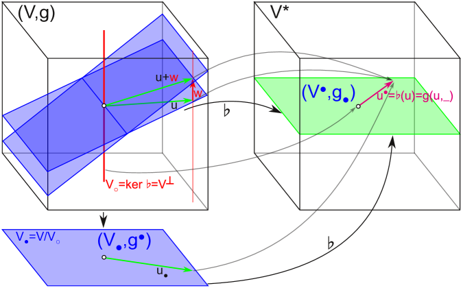
Figure 1. Various vector spaces and inner products associated with a degenerate inner product space $(V,g)$.

In figure 1, $(V,g)$ is an inner product vector space. The morphism $\flat:V\to V^{*}$ is defined by $u\mapsto u{}^{\bullet}{}:=\flat(u)=u^{\flat}=g(u,\_)$. The radical $V{}_{\circ}{}:=\ker\flat=V^{\perp}$ is the set of isotropic vectors in $V$. $V{}^{\bullet}{}:=\textnormal{im }{\flat}\leq V^{*}$ is the image of $\flat$. The inner product $g$ induces on $V{}^{\bullet}{}$ an inner product defined by $g{}_{\bullet}{}(u_{1}^{\flat},u_{1}^{\flat}):=g(u_{1},u_{2})$, which is the inverse of $g$ iff $\det g\neq 0$. The quotient $V{}_{\bullet}{}:=V/V{}_{\circ}{}$ consists in the equivalence classes of the form $u+V{}_{\circ}{}$. On $V{}_{\bullet}{}$, $g$ induces an inner product $g{}^{\bullet}{}(u_{1}+V{}_{\circ}{},u_{2}+V{}_{\circ}{}):=g(u_{1},u_{2})$.

2.2. Relations between the various spaces

The relations between the radical, the radical annihilator and the factor spaces can be collected in the diagram [14]:

where $V{}_{\bullet}{}=V{}^{\bullet}{}^{*}=\displaystyle{\frac{V}{V{}_{\circ}{}}}$ and $V{}^{\circ}{}=V{}_{\circ}{}^{*}=\frac{V^{*}}{V{}^{\bullet}{}}$.

2.3. Covariant derivative

2.3.1. The Koszul form

The Koszul form is defined as $\mathcal{K}:\mathfrak{X}(M)^{3}\to\mathbb{R}$,

(6) $$\begin{array}[]{llll}\mathcal{K}(X,Y,Z)&:=&\displaystyle{\frac{1}{2}}\{X\langle Y,Z\rangle+Y\langle Z,X\rangle-Z\langle X,Y\rangle\\ &&\ -\langle X,[Y,Z]\rangle+\langle Y,[Z,X]\rangle+\langle Z,[X,Y]\rangle\}.\end{array}$$

In local coordinates it is the Christoffel’s symbols of the first kind:

(7) $$\mathcal{K}_{abc}=\mathcal{K}(\partial_{a},\partial_{b},\partial_{c})=\displaystyle{\frac{1}{2}}(\partial_{a}g_{bc}+\partial_{b}g_{ca}-\partial_{c}g_{ab})=\Gamma_{abc},$$

For non-degenerate metrics, the Levi-Civita connection is obtained uniquely:

(8) $${\color[rgb]{1,0,0}\nabla_{X}{Y}}=\mathcal{K}(X,Y,\_)^{{\color[rgb]{1,0,0}\sharp}}.$$

For degenerate metrics, we will have to avoid the usage of the Levi-Civita connection, and limit ourselfs to using the Koszul form as much as possible.

2.3.2. The covariant derivatives

The lower covariant derivative of a vector field $Y$ in the direction of a vector field $X$ [8]:

(9) $$(\nabla^{\flat}_{X}{Y})(Z):=\mathcal{K}(X,Y,Z)$$

If the Koszul form satisfies the condition that $\mathcal{K}(X,Y,W)=0$ whenever the vector field $W$ satisfies $W\in\Gamma(T{}_{\circ}{}M)$, the singular semi-Riemannian manifold $(M,g)$ is named radical stationary.

The covariant derivative of differential forms can be defined :

$$\left(\nabla_{X}\omega\right)(Y):=X\left(\omega(Y)\right)-\langle\!\langle\nabla^{\flat}_{X}{Y},\omega\rangle\!\rangle{}_{\bullet}{},$$

if $\omega\in\mathcal{A}{}^{\bullet}{}(M):=\Gamma(T{}^{\bullet}{}M)$. More general,

$$\nabla_{X}(\omega_{1}\otimes\ldots\otimes\omega_{s}):=\nabla_{X}(\omega_{1})\otimes\ldots\otimes\omega_{s}+\ldots+\omega_{1}\otimes\ldots\otimes\nabla_{X}(\omega_{s})$$

If $T\in\Gamma(\otimes^{k}_{M}T{}^{\bullet}{}M)$, then the covariant derivative is

$$\begin{array}[]{lll}\left(\nabla_{X}T\right)(Y_{1},\ldots,Y_{k})&=&X\left(T(Y_{1},\ldots,Y_{k})\right)\\ &&-\sum_{i=1}^{k}\mathcal{K}(X,Y_{i},{{}_{\bullet}})T(Y_{1},,\ldots,{{}_{\bullet}},\ldots,Y_{k})\end{array}$$

2.4. Riemann curvature tensor. Semi-regular manifolds.

The Riemann curvature tensor can be defined, for a radical stationary manifold $(M,g)$, by:

(10) $$R(X,Y,Z,T)=({\nabla_{X}{{\nabla^{\flat}_{Y}}Z}})(T)-({\nabla_{Y}{{\nabla^{\flat}_{X}}Z}})(T)-(\nabla^{\flat}_{[X,Y]}{Z})(T)$$

In local coordinates, it takes the form:

(11) $$R_{abcd}=\partial_{a}\mathcal{K}_{bcd}-\partial_{b}\mathcal{K}_{acd}+(\mathcal{K}_{ac{{}_{\bullet}}}\mathcal{K}_{bd{{}_{\bullet}}}-\mathcal{K}_{bc{{}_{\bullet}}}\mathcal{K}_{ad{{}_{\bullet}}})$$

The Riemann curvature is a tensor field. It has the same symmetry properties as for $\det g\neq 0$. It is radical-annihilator in each of its slots.

A singular semi-Riemannian manifold is called semi-regular [8] if:

(12) $$\nabla_{X}{\nabla^{\flat}_{Y}}Z\in\mathcal{A}{}^{\bullet}{}(M).$$

Equivalently,

(13) $$\mathcal{K}(X,Y,{{}_{\bullet}})\mathcal{K}(Z,T,{{}_{\bullet}})\in\mathscr{F}(M).$$

The Riemann curvature is smooth for semi-regular metrics.

2.5. Examples of semi-regular semi-Riemannian manifolds

The following are examples of [8, 9].

2.5.1. Isotropic singularities

Isotropic singularities have the form

$$g=\Omega^{2}\tilde{g},$$

where $\tilde{g}$ is a non-degenerate bilinear form on $M$.

2.5.2. Degenerate warped products

Degenerate warped products $B\times_{f}F$ are defined similarly to the usual warped products:

(14) $$\textnormal{d}s^{2}=\textnormal{d}s_{B}^{2}+f^{2}(p)\textnormal{d}s_{F}^{2}.$$

The difference from the non-degenerate case is that for the degenerate warped products, $f$ allowed to vanish. We can take the manifolds $B$ and $F$ to be radical stationary, and the warped product will also be radical stationary, if $\textnormal{d}f\in\mathcal{A}{}^{\bullet}{}($). If $B$ and $F$ are semi-regular, and $\textnormal{d}f\in\mathcal{A}{}^{\bullet}{}($), but also $\nabla_{X}\textnormal{d}f\in\mathcal{A}{}^{\bullet}{}($) for any vector field $X$, then $B\times_{f}F$ is semi-regular.

2.5.3. FLRW spacetimes

FLRW spacetimes are degenerate warped products:

(15) $$\textnormal{d}s^{2}=-\textnormal{d}t^{2}+a^{2}(t)\textnormal{d}\Sigma^{2}$$

(16) $$\textnormal{d}\Sigma^{2}=\displaystyle{\frac{\textnormal{d}r^{2}}{1-kr^{2}}}+r^{2}\left(\textnormal{d}\theta^{2}+\sin^{2}\theta\textnormal{d}\phi^{2}\right),$$

where $k=1$ for $S^{3}$, $k=0$ for $\mathbb{R}^{3}$, and $k=-1$ for $H^{3}$.

3. Einstein’s equation on semi-regular spacetimes

3.1. Einstein’s equation on semi-regular spacetimes

On $4$D semi-regular spacetimes Einstein tensor density $G\det g$ is smooth [8]:

(17) $$G\det g+\Lambda g\det g=\kappa T\det g,$$

or, in coordinates or local frames,

(18) $$G_{ab}\det g+\Lambda g_{ab}\det g=\kappa T_{ab}\det g,$$

It is not allowed to divide by $\det g$, when $\det g=0$.

4. Friedmann-Lemaître-Robertson-Walker spacetime

4.1. The Friedmann-Lemaître-Robertson-Walker spacetime

If $S$ is a connected three-dimensional Riemannian manifold of constant curvature $k\in\{-1,0,1\}$ (i.e. $H^{3}$,$\mathbb{R}^{3}$ or $S^{3}$) and $a\in(A,B)$, $-\infty\leq A<B\leq\infty$, $a\geq 0$, then the warped product $I\times_{a}S$ is called a Friedmann-Lemaître-Robertson-Walker spacetime.

(19) $$\textnormal{d}s^{2}=-\textnormal{d}t^{2}+a^{2}(t)\textnormal{d}\Sigma^{2}$$

(20) $$\textnormal{d}\Sigma^{2}=\displaystyle{\frac{\textnormal{d}r^{2}}{1-kr^{2}}}+r^{2}\left(\textnormal{d}\theta^{2}+\sin^{2}\theta\textnormal{d}\phi^{2}\right),$$

where $k=1$ for $S^{3}$, $k=0$ for $\mathbb{R}^{3}$, and $k=-1$ for $H^{3}$.

In general the warping function is taken $a\in\mathscr{F}(I)$ is $a>0$. Here we allow it to be $a\geq 0$, including possible singularities.

The resulting singularities are semi-regular.

4.2. Distance separation vs. topological separation

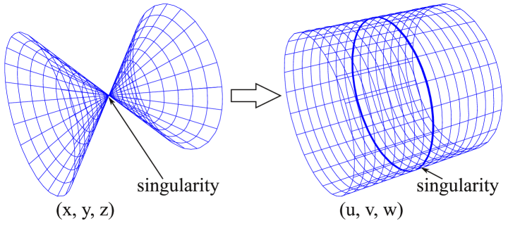
Figure 2. The old method of resolution of singularities shows how we can “untie” the singularity of a cone and obtain a cylinder. Similarly, it is not necessary to assume that, at the Big-Bang singularity, the entire space was a point, but only that the space metric was degenerate.

4.3. Friedman equations

The stress-energy tensor for a fluid in thermodynamic equilibrium, of $\rho$ mass density and $p$ pressure density, is

(21) $$T^{ab}=\left(\rho+p\right)u^{a}u^{b}+pg^{ab},$$

where $u^{a}$ is the timelike vector field $\partial_{t}$, normalized.

The following equations follow from the above stress-energy tensor, in the case of a homogeneous and isotopic universe.

The Friedmann equation is:

(22) $$\rho=\displaystyle{\frac{3}{\kappa}}\displaystyle{\frac{\dot{a}^{2}+k}{a^{2}}}.$$

The acceleration equation is:

(23) $$\rho+3p=-\displaystyle{\frac{6}{\kappa}}\displaystyle{\frac{\ddot{a}}{a}}.$$

The fluid equation, expressing the conservation of mass-energy, is:

(24) $$\dot{\rho}=-3\displaystyle{\frac{\dot{a}}{a}}\left(\rho+p\right).$$

They are singular for $a=0$.

4.4. Friedman equations, densitized

[15]

The actual densities contain in fact $\sqrt{-g}(=a^{3}\sqrt{g_{\Sigma}})$:

(25) $$\begin{array}[]{l}\bigg{\{}\begin{array}[]{ll}\widetilde{\rho}=\rho\sqrt{-g}=\rho a^{3}\sqrt{g_{\Sigma}}\\ \widetilde{p}=p\sqrt{-g}=pa^{3}\sqrt{g_{\Sigma}}\\ \end{array}\\ \end{array}$$

The Friedmann equation (22) becomes

(26) $$\widetilde{\rho}=\displaystyle{\frac{3}{\kappa}}a\left(\dot{a}^{2}+k\right)\sqrt{g_{\Sigma}},$$

The acceleration equation (23) becomes

(27) $$\widetilde{\rho}+3\widetilde{p}=-\displaystyle{\frac{6}{\kappa}}a^{2}\ddot{a}\sqrt{g_{\Sigma}},$$

Hence, $\widetilde{\rho}$ and $\widetilde{p}$ are smooth, as it is the densitized stress-energy tensor

(28) $$T_{ab}\sqrt{-g}=\left(\widetilde{\rho}+\widetilde{p}\right)u_{a}u_{b}+\widetilde{p}g_{ab}.$$

Figure 3 represents a FLRW Big-Bang singularity for $\dot{a}(0)>0$. Figure 4 represents the case when $\dot{a}(0)=0$, $\ddot{a}(0)>0$.

Figure 3. Big Bang singularity, corresponding to $a(0)=0$, $\dot{a}(0)>0$.

Figure 4. Big Bounce, corresponding to $a(0)=0$, $\dot{a}(0)=0$, $\ddot{a}(0)>0$.

5. Black hole singularities

5.1. Schwarzschild black holes

5.2. Schwarzschild singularity is semi-regular

The Schwarzschild metric is given by:

(29) $$\textnormal{d}s^{2}=-\left(1-\displaystyle{\frac{2m}{r}}\right)\textnormal{d}t^{2}+\left(1-\displaystyle{\frac{2m}{r}}\right)^{-1}\textnormal{d}r^{2}+r^{2}\textnormal{d}\sigma^{2},$$

where

(30) $$\textnormal{d}\sigma^{2}=\textnormal{d}\theta^{2}+\sin^{2}\theta\textnormal{d}\phi^{2}$$

Let’s change the coordinates to

(31) $$\begin{array}[]{l}\bigg{\{}\begin{array}[]{ll}r&=\tau^{2}\\ t&=\xi\tau^{4}\\ \end{array}\\ \end{array}$$

The four-metric becomes:

(32) $$\textnormal{d}s^{2}=-\displaystyle{\frac{4\tau^{4}}{2m-\tau^{2}}}\textnormal{d}\tau^{2}+(2m-\tau^{2})\tau^{4}\left(4\xi\textnormal{d}\tau+\tau\textnormal{d}\xi\right)^{2}+\tau^{4}\textnormal{d}\sigma^{2}$$

which is analytic and semi-regular at $r=0$ [11].

This solution can be foliated in space+time, and can therefore be used to represent evaporating black holes of Schwarzschild type. Since the solution can be analytically extended beyond the singularity, the information is not lost there (fig. 5).

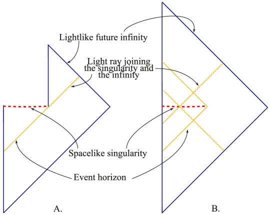
Figure 5. A. Standard evaporating black hole, whose singularity destroys the information. B. Evaporating black hole extended through the singularity preserves information.

5.3. Reissner-Nordström black holes

The Reissner-Nordström metric is given by:

(33) $$\textnormal{d}s^{2}=-\left(1-\displaystyle{\frac{2m}{r}}+\displaystyle{\frac{q^{2}}{r^{2}}}\right)\textnormal{d}t^{2}+\left(1-\displaystyle{\frac{2m}{r}}+\displaystyle{\frac{q^{2}}{r^{2}}}\right)^{-1}\textnormal{d}r^{2}+r^{2}\textnormal{d}\sigma^{2},$$

We choose the coordinates $\rho$ and $\tau$ [12], so that

(34) $$\begin{array}[]{l}\bigg{\{}\begin{array}[]{ll}t&=\tau\rho^{T}\\ r&=\rho^{S}\\ \end{array}\\ \end{array}$$

The metric has, in the new coordinates, the following form

(35) $$\textnormal{d}s^{2}=-\Delta\rho^{2T-2S-2}\left(\rho\textnormal{d}\tau+T\tau\textnormal{d}\rho\right)^{2}+\displaystyle{\frac{S^{2}}{\Delta}}\rho^{4S-2}\textnormal{d}\rho^{2}+\rho^{2S}\textnormal{d}\sigma^{2},$$

(36) $$\textnormal{where \,\,}\Delta:=\rho^{2S}-2m\rho^{S}+q^{2}.$$

To remove the infinity of the metric at $r=0$, take

(37) $$\begin{array}[]{l}\bigg{\{}\begin{array}[]{ll}S\geq 1\\ T\geq S+1\end{array}\\ \end{array}$$

which also ensure that the metric is analytic at $r=0$.

The electromagnetic potential in the coordinates $(t,r,\phi,\theta)$ is singular at $r=0$ [12]:

(38) $$A=-\displaystyle{\frac{q}{r}}\textnormal{d}t,$$

In the new coordinates $(\tau,\rho,\phi,\theta)$, the electromagnetic potential is

(39) $$A=-q\rho^{T-S-1}\left(\rho\textnormal{d}\tau+T\tau\textnormal{d}\rho\right),$$

the electromagnetic field is

(40) $$F=q(2T-S)\rho^{T-S-1}\textnormal{d}\tau\wedge\textnormal{d}\rho,$$

and they are analytic everywhere, including at the singularity $\rho=0$.

To have space+time foliation given by the coordinate, must have $T\geq 3S$ [12].

Figure 6. As one approaches the singularity on the axis $\rho=0$, the lightcones become more and more degenerate along that axis (for $T\geq 3S$ and even $S$).

6. Global hyperbolicity and information

6.1. Foliations with Cauchy hypersurfaces

If the singularities are benign, the evolution equations can make sense. But to be able to formulate initial value problems, it is needed that spacetime admits space+time foliations with respect to the metric tensor. The spacelike hypersurfaces have to be Cauchy surfaces, which is equivalent to the global hyperbolicity condition. The spacelike hypersurfaces must have the same topology for any moment of time $t$, but the metric may change its rank, and become sometimes degenerate. As we will see, the stationary black hole singularities are compatible with such foliations, hence with global hyperbolicity. Also because the topology seems to be independent on the quantities $m$, $q$, and $a$ which characterize the black hole, being their only “hair”, it is possible by varying these quantities to construct models of black holes which appear and disappear. This is relevant to evaporating black holes, since now we can see that the information is not necessarily lost.

6.2. Space-like foliation of the Reissner-Nordström solution

We can foliate the Reissner-Nordström solution in Cauchy hypersurfaces, if it is expressed in the new coordinates [12, 16, 17]. Figure 7 illustrates such a situation.

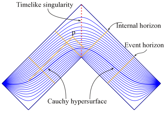
Figure 7. Foliation of the Reissner-Nordström solution in Cauchy hypersurfaces. The spacetime regions beyond the Cauchy horizons are ignored, to obtain a global foliation.

Similar foliations were obtained for the extremal and naked Reissner-Nordström black holes, as well as for the Schwarzschild and Kerr-Newman black holes.

Implications: we can vary $m$, $q$, $a$ and obtain general singularities which preserve information.

7. The mathematics of singularities 2

7.1. The Ricci decomposition

The Riemann curvature tensor can be decomposed algebraically as

(41) $$R_{abcd}=S_{abcd}+E_{abcd}+C_{abcd}$$

where

(42) $$S_{abcd}=\displaystyle{\frac{1}{n(n-1)}}R(g\circ g)_{abcd}$$

(43) $$E_{abcd}=\displaystyle{\frac{1}{n-2}}(S\circ g)_{abcd}$$

(44) $$S_{ab}:=R_{ab}-\displaystyle{\frac{1}{n}}Rg_{ab}$$

where the Kulkarni-Nomizu product is used:

(45) $$(h\circ k)_{abcd}:=h_{ac}k_{bd}-h_{ad}k_{bc}+h_{bd}k_{ac}-h_{bc}k_{ad}$$

If the Riemann curvature tensor on a semi-regular manifold $(M,g)$ admits such a decomposition which is smooth, $(M,g)$ is said to be quasi-regular.

7.2. The expanded Einstein equation

[10]

In dimension $n=4$ we introduce the expanded Einstein equation

(46) $$(G\circ g)_{abcd}+\Lambda(g\circ g)_{abcd}=\kappa(T\circ g)_{abcd}$$

or, equivalently,

(47) $$2E_{abcd}-3S_{abcd}+\Lambda(g\circ g)_{abcd}=\kappa(T\circ g)_{abcd}.$$

It is equivalent to Einstein’s equation if the metric is non-degenerate.

7.3. Examples of quasi-regular singularities

[10]

• Isotropic singularities.

• Degenerate warped products $B\times_{f}F$ with $\dim B=1$ and $\dim F=3$.

• In particular, FLRW singularities [18].

• Schwarzschild singularities.

• The question whether the Reissner-Nordström and Kerr-Newman singularities are semi-regular, or quasi-regular, is still open.

7.4. The Weyl tensor at quasi-regular singularities

[19]

The Weyl curvature tensor:

(48) $$C_{abcd}=R_{abcd}-S_{abcd}-E_{abcd}.$$

$C_{abcd}\to 0$ as approaching a quasi-regular singularity.

Because of this, any quasi-regular Big Bang satisfies the Weyl curvature hypothesis, emitted by Penrose to explain the low entropy at the Big Bang.

8. Dimensional reduction and QFT

8.1. Hints of dimensional reduction in QFT and QG

Various results obtained in QFT and in Quantum Gravity suggest that at small scales there should take place a dimensional reduction. The explanation of this reduction differs from one approach to another. Examples of such results are given below:

• The scattering amplitudes in QCD [20, 21, 22].

• High energy Regge regime [23, 24].

• Fractal universe [25, 26, 27].

• Topological dimensional reduction [28, 29, 30, 31, 32].

• Vanishing Dimensions at LHC [33].

• Dimensional reduction in Quantum Gravity [34, 35, 36].

• Asymptotic safety [37].

• Causal dynamical triangulations [38, 39, 40, 41, 42].

• Hořava-Lifschitz gravity [43].

8.2. Is dimensional reduction due to the benign singularities?

We will make some connections between these results and the benign singularities [44].

First, at each point where the metric becomes degenerate, a geometric, or metric reduction takes place, because the rank of the metric is reduced:

(49) $$\dim{T_{p}{}_{\bullet}{}M}=\dim{T_{p}{}^{\bullet}{}M}=\textnormal{rank }g_{p}.$$

This is in fact a local effect (it goes on an entire neighborhood of that point), in the regions of constant signature of the metric. This follows from the Kupeli theorem [45]: for constant signature, the space is locally a product $M=P\times_{0}N$ between a manifold of lower dimension $P$ and another manifold $N$ with metric $0$. This suggests a connection with the topological dimensional reduction explored by D.V. Shirkov and P. Fiziev [28, 29, 30, 31, 32].

If the singularity is quasi-regular, the Weyl tensor $C_{abcd}\to 0$ as approaching a quasi-regular singularity. This implies that the local degrees of freedom vanish, i.e. the gravitational waves for GR and the gravitons for QG [34].

In [12] we obtained new coordinates, which make the Reissner-Nordström metric analytic at the singularity. In these coordinates, the metric is

(50) $$\textnormal{d}s^{2}=-\Delta\rho^{2T-2S-2}\left(\rho\textnormal{d}\tau+T\tau\textnormal{d}\rho\right)^{2}+\displaystyle{\frac{S^{2}}{\Delta}}\rho^{4S-2}\textnormal{d}\rho^{2}+\rho^{2S}\textnormal{d}\sigma^{2}.$$

A charged particle can be viewed, at least classically, as a Reissner-Nordström black hole. The above metric reduces its dimension to dim $=2$.

To admit space+time foliation in these coordinates, we should take $T\geq 3S$. Is this anisotropy connected to Hořava-Lifschitz gravity?

In the fractal universe approach [25, 26, 27], one expresses the measure in

(51) $$S=\int_{\mathcal{M}}\textnormal{d}\varrho(x)\,\mathcal{L}$$

in terms of some functions $f_{(\mu)}(x)$, some of them vanishing at low scales:

(52) $$\textnormal{d}\varrho(x)=\prod_{\mu=0}^{D-1}f_{(\mu)}(x)\,\textnormal{d}x^{\mu}$$

In Singular General Relativity,

(53) $$\textnormal{d}\varrho(x)=\sqrt{-\det g}\textnormal{d}x^{D},$$

If the metric is diagonal in the coordinates $(x^{\mu})$, then we can take

(54) $$f_{(\mu)}(x)=\sqrt{\left|g_{\mu\mu}(x)\right|}.$$

This suggests that the results obtained by Calcagni by considering the universe to be fractal follow naturally from the benign metrics.

8.3. How can dimension vary with scale?

Dimension vary with distance. But how can it vary with scale? A (still very vague) answer can be the following: metric’s average determinant decreases as the number of singularities (particles) in the region increases. We conjecture that this happens and gives the regularization [44] (see fig. 8).

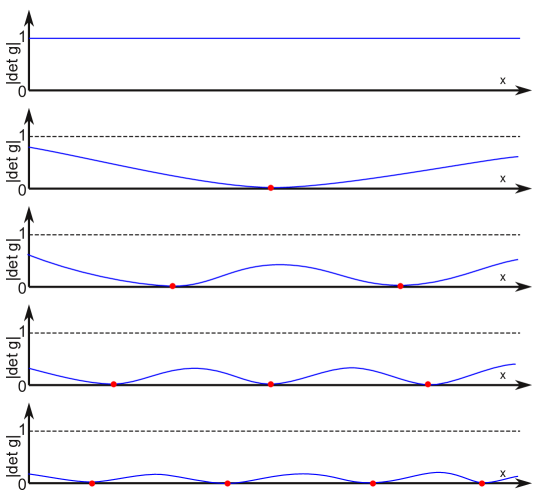
Figure 8. A conjecture: Metric’s average determinant decreases as the number of singularities (particles) in the region increases.

References

- [1] R. Penrose. Gravitational Collapse and Space-Time Singularities. Phys. Rev. Lett., (14):57–59, 1965.
- [2] S. Hawking. The occurrence of singularities in cosmology. Proceedings of the Royal Society of London. Series A. Mathematical and Physical Sciences, 294(1439):511–521, 1966.
- [3] S. Hawking. The occurrence of singularities in cosmology. ii. Proceedings of the Royal Society of London. Series A, Mathematical and Physical Sciences, pages 490–493, 1966.
- [4] S. Hawking. The occurrence of singularities in cosmology. iii. causality and singularities. Proceedings of the Royal Society of London. Series A. Mathematical and Physical Sciences, 300(1461):187–201, 1967.
- [5] S. Hawking and R. Penrose. The Singularities of Gravitational Collapse and Cosmology. Proc. Roy. Soc. London Ser. A, (314):529–548, 1970.
- [6] G. ’t Hooft and M. Veltman. One loop divergencies in the theory of gravitation. In Annales de l’Institut Henri Poincaré: Section A, Physique théorique, volume 20, pages 69–94. Institut Henri Poincaré, 1974.
- [7] M.H. Goroff and A. Sagnotti. The ultraviolet behavior of Einstein gravity. Nuclear Physics B, 266(3-4):709–736, 1986.
- [8] C. Stoica. On Singular Semi-Riemannian Manifolds. May 2011. arXiv:math.DG/1105.0201.
- [9] C. Stoica. Warped Products of Singular Semi-Riemannian Manifolds. May 2011. arXiv:math.DG/1105.3404.
- [10] C. Stoica. Einstein equation at singularities. March 2012. arXiv:gr-qc/1203.2140.
- [11] C. Stoica. Schwarzschild Singularity is Semi-Regularizable. Eur. Phys. J. Plus, (2012) 127: 83. arXiv:gr-qc/1111.4837.
- [12] C. Stoica. Analytic Reissner-Nordström Singularity. Phys. Scr., 85:055004, 2012. arXiv:gr-qc/1111.4332.
- [13] C. Stoica. Kerr-Newman Solutions with Analytic Singularity and no Closed Timelike Curves. November 2011. arXiv:gr-qc/1111.7082.
- [14] C. Stoica. Tensor Operations on Degenerate Inner Product Spaces . December 2011. arXiv:gr-qc/1112.5864.
- [15] C. Stoica. Big Bang singularity in the Friedmann-Lemaitre-Robertson-Walker spacetime. December 2011. arXiv:gr-qc/1112.4508.
- [16] C. Stoica. Globally Hyperbolic Spacetimes with Singularities. August 2011. arXiv:math.DG/1108.5099.
- [17] C. Stoica. Spacetimes with Singularities. An. Şt. Univ. Ovidius Constanţa, 20(2):213–238, July 2012. http://www.anstuocmath.ro/mathematics/pdf26/Art16.pdf.
- [18] C. Stoica. Beyond the Friedmann-Lemaitre-Robertson-Walker Big Bang singularity. March 2012. arXiv:gr-qc/1203.1819.
- [19] C. Stoica. On the Weyl Curvature Hypothesis. March 2012. arXiv:gr-qc/1203.3382.
- [20] LN Lipatov. Massless particle bremsstrahlung theorems for high-energy hadron interactions. Nuclear Physics B, 307(4):705–720, 1988.
- [21] LN Lipatov. Review in Perturbative QCD, ed. AH Mueller, 1989.
- [22] LN Lipatov. High-energy scattering in QCD and in quantum gravity and two-dimensional field theories. Nuclear Physics B, 365(3):614–632, 1991.
- [23] H. Verlinde and E. Verlinde. QCD at high energies and two-dimensional field theory. arXiv:hep-th/9302104, 1993.
- [24] I.Y. Aref’eva. Regge regime in QCD and asymmetric lattice gauge theory. Physics Letters B, 325(1):171–182, 1994.
- [25] G. Calcagni. Quantum field theory, gravity and cosmology in a fractal universe. Journal of High Energy Physics, 2010(3):1–38, 2010. arXiv:hep-th/1001.0571.
- [26] G. Calcagni. Fractal universe and quantum gravity. Physical review letters, 104(25):251301, 2010. arXiv:hep-th/0912.3142.
- [27] G. Calcagni. Gravity on a multifractal. Physics Letters B, 2011. arXiv:hep-th/1012.1244.
- [28] D.V. Shirkov. Coupling running through the looking-glass of dimensional reduction. Phys. Part. Nucl. Lett., 7(6):379–383, 2010. arXiv:hep-th/1004.1510.
- [29] P.P. Fiziev and D.V. Shirkov. Solutions of the Klein-Gordon equation on manifolds with variable geometry including dimensional reduction. Theoretical and Mathematical Physics, 167(2):680–691, 2011. arXiv:hep-th/1009.5309.
- [30] P.P. Fiziev. Riemannian (1+d)-Dim Space-Time Manifolds with Nonstandard Topology which Admit Dimensional Reduction to Any Lower Dimension and Transformation of the Klein-Gordon Equation to the 1-Dim Schrödinger Like Equation. arXiv:math-ph/1012.3520, 2010.
- [31] P.P. Fiziev and D.V. Shirkov. The (2+1)-dim Axial Universes – Solutions to the Einstein Equations, Dimensional Reduction Points, and Klein–Fock–Gordon Waves. J. Phys. A, 45(055205):1–15, 2012. arXiv:gr-qc/arXiv:1104.0903.
- [32] D.V. Shirkov. Dream-land with Classic Higgs field, Dimensional Reduction and all that. In Proceedings of the Steklov Institute of Mathematics, volume 272, pages 216–222, 2011.
- [33] L. Anchordoqui, D.C. Dai, M. Fairbairn, G. Landsberg, and D. Stojkovic. Vanishing dimensions and planar events at the LHC. arXiv:hep-ph/1003.5914, 2010.
- [34] S. Carlip. Lectures in (2+ 1)-dimensional gravity. J.Korean Phys.Soc, 28:S447–S467, 1995. arXiv:gr-qc/9503024.
- [35] S. Carlip, J. Kowalski-Glikman, R. Durka, and M. Szczachor. Spontaneous dimensional reduction in short-distance quantum gravity? In Aip Conference Proceedings, volume 31, page 72, 2009.
- [36] S. Carlip. The Small Scale Structure of Spacetime. arXiv:gr-qc/1009.1136, 2010.
- [37] S. Weinberg. Ultraviolet divergences in quantum theories of gravitation. In General relativity: an Einstein centenary survey, volume 1, pages 790–831, 1979.
- [38] J. Ambjørn, J. Jurkiewicz, and R. Loll. Nonperturbative Lorentzian path integral for gravity. Physical Review Letters, 85(5):924–927, 2000. arXiv:hep-th/0002050.
- [39] J. Ambjørn, J. Jurkiewicz, and R. Loll. Emergence of a 4D world from causal quantum gravity. Physical Review Letters, 93(13):131301, 2004. arXiv:hep-th/0404156.
- [40] J. Ambjørn, J. Jurkiewicz, and R. Loll. Reconstructing the universe. Physical Review D, 72(6):064014, 2005. arXiv:hep-th/0505154.
- [41] J. Ambjørn, J. Jurkiewicz, and R. Loll. Spectral dimension of the universe. Physical review letters, 95(17):171301, 2005. arXiv:hep-th/0505113.
- [42] J. Ambjørn, J. Jurkiewicz, and R. Loll. Quantum gravity, or the art of building spacetime. In Daniele Oriti, editor, Approaches to Quantum Gravity: Toward a New Understanding of Space, Time and Matter, pages 341–359. Cambridge University Press, 2009. arXiv:hep-th/0604212.
- [43] P. Hořava. Quantum Gravity at a Lifshitz Point. Physical Review D, 79(8):084008, 2009. arXiv:hep-th/0901.3775.
- [44] C. Stoica. Quantum Gravity from Metric Dimensional Reduction at Singularities. May 2012. arXiv:gr-qc/1205.2586 .
- [45] D. Kupeli. Degenerate Manifolds. Geom. Dedicata, 23(3):259–290, 1987.