The Evolution and Star Formation History of M33

Abstract

We construct a parameterized model to explore the main properties of the star formation history of M33. We assume that the disk originates and grows by the primordial gas infall and adopt the simple form of gas accretion rate with one free parameter, the infall time-scale. We also include the contribution of gas outflow process. A major update of the model is that we adopt a molecular hydrogen correlated star formation law and calculate the evolution of the atomic and molecular gas separately. Comparisons between the model predictions and the observational data show that the model predictions are very sensitive to the adopted infall time-scale, while the gas outflow process mainly influences the metallicity profile. The model adopting a moderate outflow rate and an inside-out formation scenario can be in good agreement with most of observed constraints of M33 disk. We also compare the model predictions based on the molecular hydrogen correlated star formation law and that based on the Kennicutt star formation law. Our results imply that the molecular hydrogen correlated star formation law should be preferred to describe the evolution of the M33 disk, especially the radial distributions of both the cold gas and the stellar population.

1 Introduction

The NGC 598 (M33) galaxy is a low-luminosity, late-type disk galaxy in the Local Group. M33 is observed to be much smaller and less massive than the Milky Way galaxy, but has much larger gas fraction. It also shows no signs of recent mergers and no presence of prominent bulge and bar component (Regan & Vogel 1994; McLean & Liu 1996). In addition, due to its proximity, large angular size, and rather low inclination, M33 is an excellent target for detailed observations of its cold gas, metallicity, the star formation rate (SFR) and stellar population, and thus provides an excellent chance for testing the model of galactic chemical evolution.

The star formation (SF) law is one of the important ingredients of the model. Based on the observed data of a sample of 97 nearby normal and star-burst galaxies, Kennicutt (1998) found a power-law correlation between the galaxy-averaged SFR surface density ($\Psi(r,t)$) and the galaxy-averaged total gas surface density ($\Sigma_{\rm gas}(r,t)$), which was termed as the classical Kennicutt SF law. Later, observations of high spatial resolution (less than kpc-scale regions) showed that the SFR surface density correlated stronger with the surface density of the molecular hydrogen ($\Sigma_{\rm H_{2}}(r,t)$) than with that of the atomic hydrogen ($\Sigma_{\rm HI}(r,t)$) and the total gas (Wong & Blitz 2002; Kennicutt et al. 2007; Bigiel et al. 2008; Leroy et al. 2008). It was also shown that the SFR surface density is almost proportional to $\Sigma_{\rm H_{2}}(r,t)$:

$$\Psi(r,t)=\Sigma_{\rm{H_{2}}}(r,t)/t_{\rm dep},$$ (1)

where $t_{\rm dep}$ is the molecular hydrogen depletion time. Hereafter, Equ. 1 is called as the $\Sigma_{\rm H_{2}}$-based SF law in this paper.

Moreover, the gas outflow process may influence the evolution of M33. Garnett (2002) concluded that spiral galaxy with $V_{\rm rot}\leq 125\rm km\,s^{-1}$ may lose some amount of gas in supernova-driven winds and Tremonti et al. (2004) also confirmed this conclusion. The results of Chang et al. (2010) indicated that the gas outflow process plays an important role in the chemical evolution of the disk galaxy since it can bring part of newly formed metal off the galactic disk. They show that the model assuming that the gas outflow efficiency increases as its stellar mass decreases can explain the observed mass-metallicity relation.

The chemical evolution of M33 has been studied by several groups in previous studies (Mollá et al. 1996; Magrini et al. 2007a; Marcon-Uchida et al. 2010). Magrini et al. (2007a) found that the model adopting an almost constant gas-infall rate can reproduce some of the observed properties of M33, especially the observed relatively high SFR and the shallow abundance gradients. Marcon-Uchida et al. (2010) compared the chemical evolution of the Milky Way, M31 and M33. They found that the model predictions of the Milky Way and that of M31 were in good agreement with the main features of observations, while the model of M33 failed to reproduce the present-day gas surface density in the inner disk. The oxygen abundance was also overestimated by 0.25 dex in the whole disk of M33.

In this paper, we build a bridge between the observed data of M33 and its star formation history (SFH) by constructing a parameterized model of its formation and evolution. A major update of the model is that we adopt the $\Sigma_{\rm H_{2}}$-based SF law and this is maybe the first time for the model of M33 to calculate separately the evolution of the atomic and molecular gas.

The paper is organized as follows. Section 2 describes the observed features of M33 disk, including the surface brightness, the SFR, the cold gas content and the metallicity etc.. The main assumptions and ingredients of our model are presented in Section 3. The comparisons between the model predictions and the observations are shown in Section 4, and Section 5 summarizes our main conclusions.

2 The Observations

In this section, we summarize the current available observations of M33 galaxy, especially the radial distributions along the disk, including the surface densities of gas and SFR, the surface brightness, the color, and the metallicity. Our model predictions will be compared with all these observed trends.

2.1 Surface brightness and radial distribution of colors

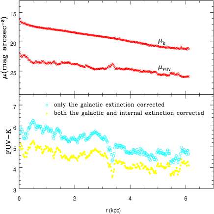
Figure 1: Surface brightness and color radial profiles of M33 disk (Muñoz-Mateos et al. 2007). upper panel: the surface brightness profiles of FUV$-$band and $K-$band. lower panel: the color profile of FUV$-K$. The observed data are described in details in Section 2.1.

Table 1. M33 disk scale-length (distance=840 kpc).
Tracer $r_{\rm d}$ (kpc) Refs. Gas ^a CO(1-0) 2.5 1 CO(1-0) 2.0 2 CO(1-0) 1.4 3 CO(2-1) 1.4 4 CO(2-1) 1.9 5 CO+21cm 7.8 ^b 1, 6 young stellar pop (0.5 $\sim$ 6 kpc) NUV 2.10 7 (Galex) FUV 2.20 7 (Galex) H_α 1.80 7, 8 B band 1.9 9 V band 1.89 10 (HST ACS) older stellar pop (0.5 $\sim$7 kpc) K band 1.00 4 (2MASS) K band 1.4 9 3.6$\,\mu$m 1.56 7 (Spitzer IRAC) 4.5$\,\mu$m 1.55 7 (Spitzer IRAC) dust, diffuse emmision (0.5 $\sim$7 kpc) 5.8$\,\mu$m 1.61 7 (Spitzer IRAC) 8.0$\,\mu$m 1.44 4, 7 (Spitzer IRAC) 24$\,\mu$m 1.55 4 (Spitzer MIPS) 24$\,\mu$m 1.40 5 (Spitzer MIPS) 24$\,\mu$m 1.77 7 (Spitzer MIPS) 60$\,\mu$m 1.30 11 (ISO) 70$\,\mu$m 1.48 5 (Spitzer MIPS) 70$\,\mu$m 1.74 7 (Spitzer MIPS) 160$\,\mu$m 1.83 5 (Spitzer MIPS) 160$\,\mu$m 1.99 7 (Spitzer MIPS) 170$\,\mu$m 1.80 11 (ISO)
a: assuming $\Sigma_{\rm gas}\propto{\rm exp}(-r/r_{\rm d})$.
b: assuming $\Sigma_{\rm gas}\propto{\rm exp}[-(r/r_{\rm d})^{2}]$.
Refs: (1) Corbelli (2003); (2) Heyer et al. (2004); (3) Engariola et al. (2003); (4) Gardan et al. (2007); (5) Gratier et al. (2010); (6) Magrini et al. (2007a); (7) Verley et al. (2009); (8) Hoopes & Walterbos (2000); (9) Regan & Vogel (1994); (10) Williams et al. (2009); (11) Hippelein et al. (2003).

The surface brightness observed in multi-bands of a galaxy contains important information of its SFH. For example, since the surface brightness in the FUV$-$band is very sensitive to the presence of recent SF activity and that in the near-infrared $K-$band strongly correlates with the accumulated SF in the galaxy, the observed radial distribution of FUV$-K$ color provides tight constraints on the specific SFR of the galaxy.

Muñoz-Mateos et al. (2007) derived the M33’s azimuthally averaged radial profiles in FUV$-K$ color by using Galaxy Evolution Explorer (GALEX) UV bands surface brightness (Gil de Paz et al. 2007) and a deep (Two-Micron All-Sky Survey) 2MASS image ($K<{\rm 21\,mag\,arcsec^{-2}}$). We show the measured FUV$-$band and $K-$band surface brightness as well as the FUV$-K$ color profiles from Muñoz-Mateos et al. (2007) in Fig. 1. In the upper panel, we plot the surface brightness of FUV$-$band and $K-$band as the red crosses which have been corrected only for the Galactic extinction. The lower panel shows the radial profiles of FUV$-K$ color, the cyan open circles have been only corrected for the Galactic extinction, and the yellow filled circles have been corrected for the both Galactic and internal extinction. It can be seen from Fig. 1 that the negative gradient (after the extinction correction) implies an inside-out formation process, that is, the stellar populations become relatively blue and young as the radius increases.

The disk scale-length $r_{\rm d}$ can be obtained from radial profile, but it has some complexity since it is not only dependent on the wavelength, but also related to what we refer: gas disk, stellar disk or the total. Based on the surface brightness profiles in $B$ and $K$ bands, Regan & Vogel (1994) derived a stellar scale-length of $1.9\rm\,kpc$ and 1.4$\rm\,kpc$ respectively. While the CO (representing the molecular hydrogen distribution) radial scale-length is about $2.5\rm\,kpc$ (Corbelli 2003), larger than that of the stellar disk. When the total gas mass surface density ($\Sigma_{\rm H_{2}}+\Sigma_{\rm HI}$) is concerned, the resulted scale-length is much larger (Corbelli 2003; Magrini et al. 2007a). In Table 1, we list the scale-length for different disk components of the M33. In general, the $K-$band luminosity reflects the stellar profile, a smaller value of $r_{\rm d,K}$ implies that the stellar disk is more concentrated than the gas disk. In this paper we will adopt $r_{\rm d}=1.4\rm\,kpc$ (Regan & Vogal 1994). The total stellar mass of M33 is estimated to be $\sim(3.0-6.0)\times 10^{9}\,{\rm M}_{\odot}$ (Corbelli 2003).

2.2 Profiles of cold gas, SFR and gas depletion time

During the past years, a number of data sets relating to the atomic and molecular gas distributions in M33 are becoming available. Imaging of molecular clouds has recently been carried out in M33 with the Berkeley-Illinois-Maryland Association (BIMA) interferometer and with the Five College Radio Astronomy Observatory (FCRAO) 14m telescope using the CO $J=1-0$ line transition (Corbelli 2003; Engargiola et al. 2003; Heyer et al. 2004; Verley et al. 2009). It was also observed by the Institute de RadioAstronomie Millimétrique (IRAM) 30m telescope using the CO $J=2-1$ line transition (Gardan et al. 2007; Gratier et al. 2010). The observed radial profiles of H₂ surface density are plotted in the top panel of Fig. 2, where the data are taken from Corbelli (2003) (the green filled triangles), Heyer et al. (2004) (the cyan filled squares), Verley et al. (2009) (the red filled circles (FCRAO)), and Gratier et al. (2010) (the blue asterisks).

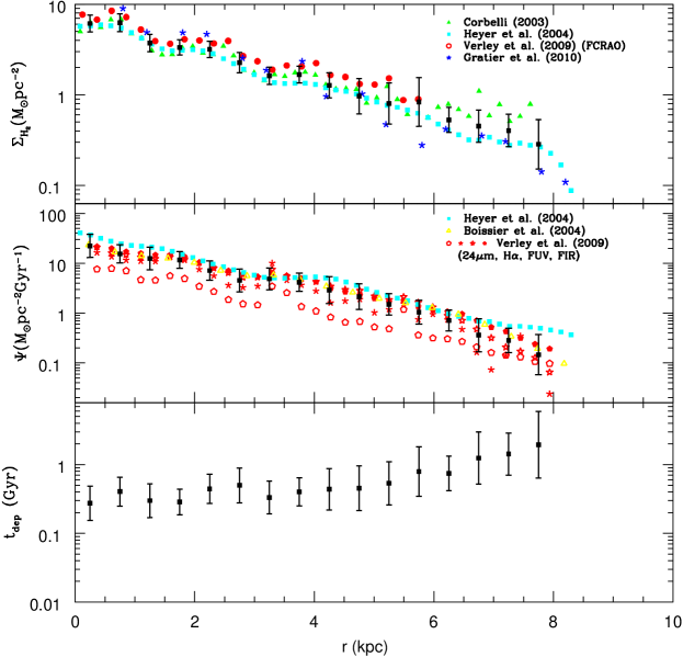
Figure 2: Observed profiles of the surface density of $\rm H_{2}$ and SFR, and the molecular gas depletion time for M33 disk. top panel: current surface density profiles of $\rm H_{2}$. middle panel: current surface density profiles of SFR. The mean values of both $\Psi(r,t)$ and $\Sigma_{\rm H_{2}}$ in each bin are shown as filled squares with error bars, where the error bars represent the distribution dispersion in each bin. bottom panel: the filled squares are the molecular gas depletion time estimated according to the $\Sigma_{\rm H_{2}}$-based SF law, and the error bars also represent the distribution dispersion in each bin. The observed data are described in details in Section 2.2.

The cold gas distribution is tightly correlated with the distribution of the SFR. Several groups have already measured the SFR in several regions along the disk of M33 using different tracers, including the H$\alpha$ emission, the luminosity in the far-ultraviolet (FUV) band and the far-infrared (FIR) band (Hippelein et al. 2003; Engargiola et al. 2003; Heyer et al. 2004; Gardan et al. 2007; Boissier et al. 2007; Verley et al. 2009). The observed data of the radial distribution of the SFR surface densities are plotted in the middle panel of Fig. 2. The data taken from Heyer et al. (2004) and Boissier et al. (2007) are shown by the cyan filled squares (FIR) and the yellow empty triangles (FUV), respectively. The data taken from Verley et al. (2009) are represented by the red empty pentagons (24$\,\rm\mu m$), the red asterisks (H$\alpha$), the red five-pointed stars (FUV), and the red filled pentagon (FIR).

Since the observed SFR surface density $\Psi(r,t)$ and the molecular hydrogen surface density $\Sigma_{\rm H_{2}}(r,t)$ are both available, it is easy to estimate the molecular gas depletion time $t_{\rm dep}$ according to the $\Sigma_{\rm H_{2}}$-based SF law. In practice, we first divide the observed data along the disk of M33 into 16 bins. Then, we calculate the mean values of both $\Psi(r,t)$ and $\Sigma_{\rm H_{2}}(r,t)$ in each bin in the logarithmic coordinates and show them as filled squares with error bars in top and middle panels of Fig. 2, where the error bars represent the distribution dispersion in each bin. Using the mean values obtained, we calculate the molecular gas depletion time in each bin through $t_{\rm dep}=\Sigma_{\rm H_{2}}(r,t)/\Psi(r,t)$ (according to the $\Sigma_{\rm H_{2}}$-based SF law) and plot them in the bottom panel of Fig. 2 as filled squares with error bars. It can be seen that $t_{\rm dep}$ is almost constant along the most part of the disk except in the outer region of the disk ($r>4r_{\rm d}$), where $t_{\rm dep}$ increases gradually as the galactic radius increases. For the purpose of simplicity, we adopt the mean value of the molecular gas depletion time and fix $t_{\rm dep}=0.43\,\rm{Gyr}$ throughout this work.

The reciprocal quantity of the molecular gas depletion time $1/t_{\rm dep}$ of a galaxy correlates to its star formation efficiency (SFE), which describes the proportion of molecular gas turns into stellar mass in unit time. Leroy et al. (2008) explored the SFEs of 23 nearby galaxies, and they estimated that the average value of $t_{\rm dep}$ is about $1.9\,\rm{Gyr}$ in large spirals. However, the case of M33 is slightly different. Gardan et al. (2007) found that M33 was more efficient in forming stars than large spirals in the local universe and the molecular depletion time was about $0.11-0.32\,\rm{Gyr}$. Gratier et al. (2010) also concluded that the SFE of M33 appeared to be 2-4 times higher than that observed in massive spiral galaxies. Our results of Fig. 2 also suggest that the SFE of M33 is almost constant along the disk and higher than the average value of SFE of large spirals investigated by Leroy et al. (2008).

The Hi surface density profile has been derived from high sensitivity observations with the Westerbork Synthesis Radio Telescope (WSRT)+Effelsberg 100m (Deul & van der Hulst 1987), with the Arecibo (Corbelli & Schneider 1997; Putman et al. 2009) and with the Very Large Array (VLA) B, C, and D (Gratier et al. 2010).

2.3 Disk abundance gradients

Table 2. Observed abundance gradients in M33 (dlog(O/H)/dR, in $\rm dex\,kpc^{-1}$).
Objects $R_{\rm g}$ Oxygen gradient Refs. (kpc) $\rm dex\,kpc^{-1}$ Hii 1.0–5.7 $-$0.13 (1) 0.2–6.5 $-$0.070$\pm$0.008 (2) 0.4–6.5 $-$0.127$\pm$0.011 (3) 0.3–11.0 $-$0.19 $\pm$0.03 (4) 1.0–7.2 $-$0.012$\pm$0.011 (5) 2.0–7.2 $-$0.054$\pm$0.011 (6) 0.2–6.0 $-$0.027$\pm$0.012 (7) 1.0–8.0 $-$0.044$\pm$0.009 (8) PNe 1.0–10.0 $-$0.11$\pm$0.04 (9) 0.5–8.5 $-$0.031$\pm$0.013 (10) 0.5–8.0 $-$0.013$\pm$0.016 (11) B stars 0.2–4.1 $-$0.16$\pm$0.06 (12) 0.25–8.0 $-$0.06$\pm$0.02 (13)
Refs: (1) Kwitter & Aller (1981); (2) Vílchez et al. (1988); (3) Zaritsky et al. (1994); (4) Henry & Howard (1995); (5) Crockett et al. (2006); (6) Magrini et al. (2007b); (7) Rosolowsky & Simon (2008); (8) Magrini et al. (2010); (9) Magrini et al. (2007a); (10) Magrini et al. (2009); (11) Bresolin et al. (2010); (12) Monteverde et al. (1997); (13) Urbaneja et al. (2005).

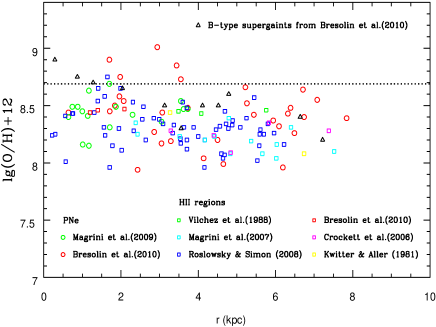
Figure 3: Observed O abundance in M33 disk. Different data notations represent those taken from various literature. Dotted line in the panel is the corresponding solar values taken from Asplund et al. (2009). The observed data are described in details in Section 2.3.

The abundance gradient is an essential ingredient in an accurate picture of galaxy formation and evolution. The existence of abundance gradient along the Milky Way has been proved by observations during the past twenty years using different tracers. An oxygen or/and iron abundance gradients about $-0.06\sim-0.07\rm\,dex\,kpc^{-1}$ were obtained by using various tracers, such as Hii regions, B stars (see Rudolph et al. 2006 and references therein), Planetary Nebulae (PNe) (Maciel et al. 2006) and open clusters (Chen et al. 2003, 2008). A radial dependent SFR and an infall model with disk formed by “inside-out” scenarios could well reproduce the above gradients (Matteucci & Francois 1989; Boissier & Prantzos 1999; Hou et al. 2000; Chiappini et al. 2001; Fu et al. 2009; Yin et al. 2009).

Nevertheless, the abundance gradients for different elements are different, and the exact gradient value, especially its time evolution, for the Milky Way disk are still not very certain. This has prevented from a clear constraint for the chemical evolution models. Therefore it is very important to have more data from extragalactic galaxies. Indeed, abundance gradients have been found in many other spiral galaxies (Zaritsky et al. 1994). At present, the best studied extragalactic galaxies for abundance is the M101 (Kennicutt et al. 2003), M31 and M33 (Rosolowsky & Simon 2008; Magrini et al. 2007b) by observing a large sample of Hii regions and young stars in their disks.

The observed abundance gradient of Hii regions in M33 have been obtained by several authors. First quantitative spectroscopic studies were carried out by Smith (1975), Kwitter & Aller (1981), and Vílchez et al. (1988). These observations, which were limited to the brightest and largest Hii regions, implied a steep radial oxygen gradient about $-0.1\rm\,dex\,kpc^{-1}$. Using the data from previous observations with derived electron temperatures, Garnett et al. (1997) re-determined the radial oxygen abundance and obtained an overall oxygen gradient of $-0.11\pm 0.02\rm\,dex\,kpc^{-1}$, including the central regions of M33. Recent studies seemed to converge to a much shallower gradients, such as Crockett et al. (2006), Magrini et al. (2007b) (hereafter M07b), Rosolowsky & Simon (2008) (hereafter RS08) and Magrini et al. (2010), deriving the radial oxygen gradients as $-0.012\pm 0.011\rm\,dex\,kpc^{-1}$, $-0.054\pm 0.011\rm\,dex\,kpc^{-1}$, $-0.027\pm 0.012\rm\,dex\,kpc^{-1}$, and $-0.044\pm 0.009\rm\,dex\,kpc^{-1}$, respectively.

Using PNe spectroscopy, Magrini et al. (2004) measured the element abundances of 11 PNe in M33. Magrini et al. (2007a; hereafter M07a) derived an oxygen radial gradient of $-0.11\pm 0.04\rm\,dex\,kpc^{-1}$, while Magrini et al. (2009; hereafter M09) presented a new result of $-0.031\pm 0.013\rm\,dex\,kpc^{-1}$ from 91 PNe in M33. Adding their observed data of 16 PNe to the 32 (out of 91) sample of M09, Bresolin et al. (2010) obtained an oxygen radial gradient of $-0.013\pm 0.016\rm\,dex\,kpc^{-1}$ from this combined sample.

Abundance gradients in M33 disk have also been estimated from B-type giants, for example, Monteverde et al. (1997) derived the oxygen radial gradient of $-0.16\pm 0.06\rm\,dex\,kpc^{-1}$, and Urbaneja et al. (2005) obtained the oxygen radial gradient of $-0.06\pm 0.02\rm\,dex\,kpc^{-1}$.

Clearly, the true situation of the abundance gradient in M33 disk is still not fixed. Optical line spectroscopy are mainly concentrated on the B stars, Hii regions. The main uncertainty comes from the empirical calibrations which are used to derive the electron temperatures in the nebular. And the stellar data suffers from lack of enough sample. Also the derived abundance gradient depends on the distance ranges. In any case, a larger and homogeneous sample of Hii regions which spread the whole M33 disk is needed in order to have conclusive results about the real gradients. Such project is currently undergoing by a couple of groups (Rosolowsky & Simon 2008; Magrini et al. 2007b).

In Table 2, we present most currently available oxygen abundance gradient measurements for M33 disk. We plot the oxygen abundance observed in PNe, Hii regions and B-type super-giants along the disk in Fig. 3. The observed data derived through PNe are denoted by open circles, where the 32 (out of 91) red open circles are taken from M09 and the 16 green ones are taken from Bresolin et al. (2010). The open squares represent the observed data obtained though Hii regions, where the blue, the cyan, the green, the yellow, the magenta and the red open squares are taken from RS08, M07b, Víchez et al. (1988), Kwitter & Aller (1981), Crockett et al. (2006) and Bresolin et al. (2010), respectively. In addition, the observed data estimated from B-type super-giants are shown in the same panel via black empty triangles. In order to compare model predictions with the observations, these data are also plotted in the left-bottom panel of Fig. 4.

A clear property from Fig. 3 is that the M33 disk has a sub-solar overall metallicity. It is consistent with the fact that low mass galaxies have lower metallicity than the high mass system, following the mass-metallicity relation among galaxies (Tremonti et al. 2004 ). Physically, the low metal content in low mass galaxies can be interpreted as the role of either the large gas accretion (infall) or the strong galactic winds (outflow), because both can change the metallicity of the galaxy disk and gas fraction (Dalcanton 2007). Since M33 is a low mass system, we have reasons to assume that M33 is undergoing substantial galactic outflow processes during its evolution.

3 The Model

Motivated by various observed properties available along the M33 disk, we build a bridge between the observations of M33 and its SFH by constructing a chemical evolution model. We assume that the disk has been embedded in a dark matter halo. Primordial gas ($X=0.7571,Y_{\rm p}=0.2429,Z=0$) within the dark halo cools down gradually to form a rotationally supported disk. The disk is basically assumed to be sheet-like and composed by a series of independent rings with the width of 500 pc. Since radial flows are still in the stage of lacking a well understood description and will bring additional free parameters and uncertainties in the model, we do not consider radial flows in this paper. The details and essentials of our model are as follows.

3.1 Gas infall rate

The gas infall process has been introduced in the formation model of the Milky Way disk due to the well-known “G-dwarf problem”, which means that the simple “closed-box” model cannot explain the locally observed metallicity distribution function of long-lived stars (Pagel 1989). Recent observations, which were detected at 21-cm by Westmeier et al. (2005), also showed that the M33 disk is still in the process of accreting substantial gas.

We assume that the M33 disk is progressively built up by the infall of primordial gas from its dark matter halo. For the given radius $r$, the gas infall rate $f_{\rm{in}}(r,t)$ (in units of $\rm{M_{\odot}}\,{pc}^{-2}\,{Gyr}^{-1}$) is assumed to be:

$$f_{\rm{in}}(r,t)=A(r)\cdot t\cdot e^{-t/\tau},$$ (2)

where $\tau$ is the infall time-scale and it is a free parameter in our model. The $A(r)$ are actually a set of separate quantities constrained by the stellar mass surface density at the present time. In practice, we iteratively estimate $A(r)$ by requiring the model resulted stellar mass surface density at the present time is equal to its observed value (Chang et al. 2010, 2012). The stellar disk of M33 is described by an exponential surface density profile and given by

$$\Sigma_{*}(r,t_{\rm g})=\Sigma_{*}(0,t_{\rm g}){\rm exp}{(-r/r_{\rm d})},$$ (3)

where $\Sigma_{*}(r,t_{\rm g})$ is the stellar mass surface density at the present time. $t_{\rm g}$ is the cosmic age and we set $t_{\rm g}=13.5\rm\,Gyr$ according to the standard cosmology. $\Sigma_{*}(0,t_{\rm g})$ is the central stellar mass surface density at the present time. $r_{\rm d}$ is the radial scale-length of the stellar disk and we set $r_{\rm d}=1.4\,\rm{kpc}$. The total stellar mass of the M33 disk is given by

$$M_{*}(t_{g})=\Sigma_{*}(0,t_{\rm g})2\pi r_{\rm d}^{2}.$$ (4)

We adopt $M_{*}(t_{\rm g})=4.0\times 10^{9}\,{\rm M}_{\odot}$ and accordingly we set $\Sigma_{*}(0,t_{\rm g})=325\rm{M_{\odot}}\,{pc}^{-2}\,$.

In previous models of the chemical evolution of disk galaxies, the gas infall rate is widely assumed to be exponentially decreasing with time (Hou et al. 2000; Chiappini et al. 2001; Yin et al. 2009). However, because of small initial mass of M33, the disk may initially accumulate a small amount of gas and its accretion rate may gradually increase as its gravitational potential builds up, and then start decreasing when the gas reservoir is depleted (Prantzos & Silk 1998). Therefore, we adopt another form of gas infall rate in this paper. Generally speaking, the gas infall rate we adopted is low at the beginning and gradually increases with time. It reaches to the maximum value when $t=\tau$ and then slowly falls down. We emphasize that the infall time-scale $\tau$ is an important free parameter in our model, which regulates the shape of gas accretion history and then largely influences the main properties of SFH along the disk.

3.2 Star formation law

It is well known that almost all stars form in molecular clouds, therefore, it is natural to expect that the SFR correlates more strongly with the molecular gas surface density than with the total one. Indeed, studies of spacial resolved SF law show that the SFR correlates stronger with the surface density of molecular hydrogen rather than that of atomic hydrogen (Wong & Blitz 2002; Bigiel et al.2008; Leroy et al. 2008). In this paper, we adopt the $\Sigma_{\rm H_{2}}$-based SF law (see equ. 1). We calculate the molecular hydrogen depletion time of M33 using the observed surface density of SFR and $\rm H_{2}$ in Section 2.1 and we adopt $t_{\rm dep}=0.43\,\rm{Gyr}$ throughout this work.

Regarding the ratio of molecular to atomic gas surface density of a galaxy disk $R_{\rm mol}$, Blitz & Rosolowsky (2006) and Leroy et al. (2008) proposed that the mid-plane pressure of the interstellar medium (ISM) $P_{\rm h}$ alone could determine $R_{\rm mol}(r,t)$:

$$R_{\rm{mol}}(r,t)={\Sigma_{{{\rm{H}}_{2}}}}(r,t)/{\Sigma_{{\rm{H{\sc I}}}}(r,t)}={\left[{P_{\rm h}\left(r,t\right)/{P_{0}}}\right]^{\alpha_{P}}},$$ (5)

where $P_{0}$ and $\alpha_{\rm P}$ are constants derived from the observations. We adopt $P_{0}=4.3\times 10^{4}\,\rm{cm}^{-3}\,\rm{K}$ and $\alpha_{\rm P}=0.92$ (Blitz & Rosolowsky 2006).

According to Elmegreen (1989, 1993), the mid-plane pressure of the ISM in the disk galaxies can be expressed as:

$$P_{\rm h}\left(r,t\right)=\frac{\pi}{2}G{\Sigma_{{\rm{gas}}}}\left(r,t\right)\left[{{\Sigma_{{\rm{gas}}}}\left(r,t\right)+\frac{c_{\rm gas}}{c_{\rm star}}{\Sigma_{*}}\left(r,t\right)}\right],$$ (6)

where $G$ is the gravitational constant, $c_{\rm{gas}}$ and $c_{\rm{star}}$ are the (vertical) velocity dispersions of gas and stars, respectively. Observations suggest that $c_{\rm{gas}}$ is a constant along the disk and we adopt $c_{\rm{gas}}=11\rm\,km\,s^{-1}$ (Ostriker et al. 2010), but $c_{\rm{star}}=\sqrt{\pi Gz_{0}\Sigma_{*}(r)}$, where $z_{0}$ is the scale-height of the disk and we adopt $z_{0}=0.5\,\rm{kpc}$ (Heyer et al. 2004).

3.3 Gas outflow rate

As we have already mentioned in the previous section, the outflow process may influence the evolution of M33. Indeed, Garnett (2002) suggested that spiral galaxies with $V_{\rm rot}\leq 125\rm\,km\,s^{-1}$ may lose some amount of gas in supernova-driven winds. Spitoni et al. (2010) also concluded that the outflow may play a significant role especially for galaxies with the stellar mass less than $10^{10}\,{\rm M}_{\odot}$. To explain the observed correlation between the galactic gas-phase metallicity and its stellar mass, Tremonti et al. (2004) and Chang et al. (2010) suggested that it is necessary that the gas outflow efficiency of a galaxy may increase as the galactic stellar mass decreases. Since M33 is a low mass system with a rotation speed about $V_{\rm rot}\approx 110\rm\,km\,s^{-1}$, the gas outflow process should paly an important role in its disk evolution.

Following Chang et al. (2010), we also assume that the outflow gas has the same metallicity as that of ISM at that time and will not fall again to the disk. The gas outflow rate $f_{\rm out}(r,t)$ (in units of $\rm{M_{\odot}}\,{pc}^{-2}\,{Gyr}^{-1}$) is assumed to be proportional to the SFR surface density $\Psi(r,t)$ :

$$f_{\rm out}(r,t)=b_{\rm out}\Psi(r,t)$$ (7)

where $b_{\rm out}$ is another free parameter in our model.

3.4 Stellar evolution and chemical evolution equations

The updated stellar population synthesis (SPS) model of Bruzual & Charlot (2003), i.e., CB07, is adopted in our work, with the stellar initial mass function (IMF) being taken from Chabrier (2003). The lower and upper mass limits are adopted to be $0.1\,{\rm M}_{\odot}$ and $100\,{\rm M}_{\odot}$, respectively.

Regarding the chemical evolution of the disk of M33, both the instantaneous-recycling approximation and the instantaneous mixing of the gas with ejecta are assumed, i.e., the gas in a fixed ring is characterized by a unique composition at each epoch of time. We take the classical set of equations of galactic chemical evolution from Tinsley (1980):

$$\frac{d[\Sigma_{\rm tot}(r,t)]}{dt}=f_{\rm{in}}(r,t)-f_{\rm{out}}(r,t),$$ (8)

$$\frac{d[\Sigma_{\rm gas}(r,t)]}{dt}=-(1-R)\Psi(r,t)+f_{\rm{in}}(r,t)-f_{\rm{out}}(r,t),$$ (9)

$$\frac{d[Z(r,t)\Sigma_{\rm gas}(r,t)]}{dt}=y(1-R)\Psi(r,t)-Z(r,t)(1-R)\Psi(r,t)$$

$$+Z_{\rm{in}}f_{\rm{in}}(r,t)-Z_{\rm{out}}(r,t)f_{\rm{out}}(r,t),$$ (10)

where $\Sigma_{\rm tot}(r,t)$ is the total (star + gas) mass surface density. $Z(r,t)$ is the metallicity in the ring centered at galactocentric distance $r$ at evolution time $t$. $R$ is the return fraction and we set $R=0.3$ according to the adopted IMF. $y$ is the stellar yield and we set $y=1\,{\rm Z}_{\odot}$ (Chang et al. 2010). $Z_{\rm{in}}$ is the metallicity of the infalling gas and we assume the infalling gas is primordial, that is $Z_{\rm{in}}=0$. $Z_{\rm{out}}(r,t)$ is the metallicity of the outflowing gas and we assume that the outflow gas has the same metallicity as that of ISM, e.g., $Z_{\rm{out}}(r,t)=Z(r,t)$ (Chang et al. 2010).

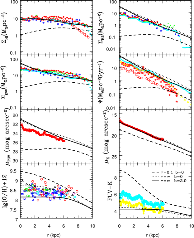
Figure 4: Influence of free parameters on the model predictions. At the left-side, from top to bottom it shows the Hi surface density, total gas surface density, surface brightness in FUV$-$band, and oxygen abundance radial profiles. At the right-side, from top to bottom it shows H₂ surface density, SFR surface density, surface brightness in $K-$band, and FUV$-K$ color radial profiles. Different line types correspond to various parameter groups: dashed lines $(\tau,b_{\rm out})=(0.1\,{\rm Gyr},0)$, dotted lines $(\tau,b_{\rm out})=(\infty$, 0), solid lines $(\tau,b_{\rm out})=(\infty$, 2). The observed data are described in details in Section 2.

In summary, two free parameters in our model are the infall time-scale $\tau$ and the outflow coefficient $b_{\rm out}$. The combination of gas infall rate and outflow rate determines the behavior the total (gas+star) mass surface density. We assume that the initial total mass surface density is zero, then we can numerically obtain the total mass surface density at any time after free parameters being given. Adding the SF law, we can easily describe how much cold gas turns into stellar mass and then numerically calculate the chemical and color evolution of the disk of M33.

4 Model Results Versus Observations

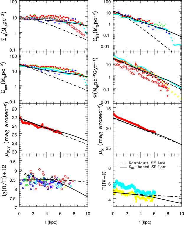
Figure 5: Comparison of the predictions of the viable model with the observations. The solid lines plot the viable model results, which adopts $(\tau,b_{\rm out})=(r/{\rm r_{d}}+5.0\,\rm{Gyr},0.5)$ and with the $\Sigma_{\rm H_{2}}$-based SF law, while the dashed lines are with the same $(\tau,b_{\rm out})$ but with the Kennicutt SF Law $\Psi(r,t)=0.25\Sigma_{\rm gas}^{1.4}(r,t)$. The observed data symbols are the same as those in Fig. 4.

Figure. 4 presents comparison between the model predictions and the observations. The left-side of Fig. 4 shows the Hi surface density, total gas surface density, surface brightness in FUV$-$band, and oxygen abundance radial profiles. The right-side shows H₂ surface density, SFR surface density, surface brightness in $K-$band, and FUV$-K$ color radial profiles, respectively. The data of observed radial profiles of Hi are taken from Corbelli (2003) (green filled triangles), Heyer et al. (2004) (cyan filled squares) and Gratier et al. (2010) (blue asterisks). The data taken from Verley et al. (2009) are shown by red empty circles (Westerbork) and filled circles (Arecibo). The left-second panel of Fig. 4 plots the total gas surface density, which is defined as $1.33(\Sigma_{\rm{H_{2}}}(r,t)+\Sigma_{\rm HI}(r,t))$ (the factor of 1.33 considers the contribution of helium), where the data notation is the same as that of H₂. The data of total gas surface density taken from Verley et al. (2009) is calculated using the Arecibo data of $\Sigma_{\rm HI}$ except for the first four inner radius, where we used the values from Westerbork. The notations of other panels of the observed data are the same as that described in details in Section 2.

We explore the influence of free parameters on model results step by step. Firstly, we do not consider the contribution of gas outflow process ($b_{\rm{out}}=0$), and explore the influence of $\tau$ on model results. The dashed and dotted lines in Fig. 4 denote the model predictions of two limiting cases of $\tau=0.1$ Gyr and $\tau\rightarrow\infty$, respectively. The case of $\tau\rightarrow 0$ corresponds to a time-declining infall rate, which is very close to the “closed-box” model, while $\tau\rightarrow\infty$ corresponds to a nearly constant with a slight time-increasing gas infall rate.

It can be seen from Fig. 4 that the model predictions are very sensitive to the adopted $\tau$. The model adopting a shorter $\tau$ predicts lower gas surface density (i.e. both Hi and H₂ components), lower SFR, lower surface brightness, redder color, and higher metallicity than that of adopting longer $\tau$. This is mainly due to the fact that, in our model, the setting of short infall time-scale corresponds to a fast gas infall process and high SF process in the early time of the galaxy evolution, and then leads to old stellar population, high metallicity and low cold gas content at the present day.

To investigate the influence of gas outflow process on the evolution of M33, the solid lines in Fig. 4 plot the model results adopting $\tau=\infty$ and $b_{\rm{out}}=2$. Comparison between solid lines and dotted lines shows that the gas outflow process has no significant influence on the stellar population and the cold gas content, but it does reduce the gas-phase metallicity since it takes a fraction of metals away from the disk. Therefore, the observed radial distribution of oxygen abundance may tightly constrain the gas outflow process of M33.

Another interesting point of Fig. 4 is that the area between the dashed and solid lines almost covers the whole region of the observations, which means that it is possible to construct an evolution model that can reproduce the main features of the observations of M33 disk. Considering the observed trends that the inner stellar disk seems to be redder and metal richer than that of the outer region, we adopt the inside-out disk formation scenario, i.e., a radial dependent infall time-scale $\tau=r/{\rm r_{d}}+5.0\,\rm{Gyr}$ and a moderate outflow rate $b_{\rm out}=0.5$ as the viable model, and its results are plotted as solid lines in Fig. 5. The observed data is the same as that of the Fig. 4. It can be seen that the solid lines are in fairy agreement with the most of observational data, which suggests that our viable model includes and reasonably describes the important ingredients of main processes that regulate the formation and evolution of the M33.

The infall time-scale is one of the important free parameters in our model. After exploring its influences on the radial profiles of M33 and computing several sets of combinations of free parameters, we finally choose the radial-dependent infall time-scale in the viable based on the balance that the model predictions can be consistent with most of the observed data. We emphasize that although the accurate values of free parameters in the viable model are not unique, the main trend that $\tau(r)$ increases from the inner disk to the outer parts are robust. In fact, this assumption is consistent with the well-known idea that the disk forms inside-out and has already applied in previous models of formation and evolution of disk galaxies (Matteucci & Francois 1989; Boissier & Prantzos 1999; Hou et al. 2000; Chiappini et al. 2001; Fu et al. 2009; Yin et al. 2009).

Figure 6: Current radial profiles of mean stellar age with different SF laws, solid line ($\Sigma_{\rm H_{2}}$-based SF law), dashed line (Kennicutt SF law).

In order to clearly demonstrate the property of the inside-out formation scenario, we plot the mean stellar age along the disk predicted by our typical model with solid lines in Fig. 6. It can be seen that the model predicts a decreasing mean stellar age from the inner disk to the outer region since the short infall time-scale means a large fraction of stars formed at early stage and hence old mean stellar age. Indeed, the ground-based observations of bright stars in M33 suggest that the outer disk of M33 may have formed at late epoch and the SF process may be on-going (Davidge 2003; Block et al. 2004; Rowe et al. 2005).

Another method to test the inside-out formation scenario is to measure the radial distribution of the mean age of the stellar populations along the disk. Williams et al. (2009) presented resolved stellar photometry of four fields along the M33 disk and found that the age of the majority of the stars decreases with increasing galactic distance, which is consistent with our model prediction. On the other hand, the investigation of stellar age distribution in far outer disk of M33 (outside the break radius $r>8\rm kpc$) shows that the mean age of stars in far outer disk is young ($\sim 3\rm Gyr$) but the age increases with radius (Barker et al. 2007; Barker et al. 2011). The explanation of the origin of this reverse age gradient in the far outer disk of M33 is still an open question and needs further investigations.

The SF law is another important components of the model that may largely influence the evolution of M33. In this paper, we adopt the $\Sigma_{\rm H_{2}}$-based SF law instead of the classic Kennicutt SF law (that is, $\Psi(r,t)=0.25\Sigma_{\rm gas}^{1.4}(r,t)$) in previous studies. We compare the model predictions when using these two kinds of SF laws in Fig. 5 and Fig. 6. The results of Kennicutt SF law are shown by dashed lines. Other ingredients of the model, including the molecular-to-atomic ratio $R_{\rm mol}$, are the same as that of the viable model. It can be seen that the solid lines are clearly distinguished from the dashed lines, especially in the outer disk where the cold gas surface density is low. Comparing to the model adopting the $\Sigma_{\rm H_{2}}$-based SF law, the model adopting the Kennicutt SF law predicts much flatter gradients of metallicity, mean stellar age and color, while steeper gradients of $\Sigma_{\rm H_{2}}$, $\Sigma_{\rm HI}$ and $\Psi(r,t)$. These results suggest that, comparing to the $\Sigma_{\rm H_{2}}$-based SF law, the SFE of Kennicutt SF law is higher in the outer regions of the disk. This means that the cold gas in the outer regions will turn into stars more efficiently, which will result in an older stellar population. Indeed, previous works on the evolution of the Milky Way and M31 disks have shown that, in order to agree with the observed metallicity gradient and its time evolution well, it is necessary to adopt a modified Kennicutt SF law, such as $\Psi(r,t)\propto\Sigma_{\rm gas}^{1.4}(r,t)/r$ (Boissier & Prantzos 1999; Chang et al 1999; Fu et al. 2009; Yin et al. 2009). However, why the SFE should be inversely correlated directly with the galactic radius is not fully understood. Our results show that the model predictions based on the $\Sigma_{\rm H_{2}}$-based SF law are more consistent with observed trends, especially the radial distributions of both the cold gas and the stellar population.

5 Summary

In this paper, we construct a parameterized model of the formation and evolution of M33 disk by assuming that the disk originates and grows by the primordial gas infall. The gas infall rate is described by a simple formula with one free parameter, the infall time-scale $\tau$. We also include the contribution of gas outflow. A molecular hydrogen correlated SF law is adopted to describe how much the cold gas turns into the stellar mass. We numerically calculate the evolution of M33 and compare the model predictions with the observational data.

The main results of our model can be summarized as follows:

1. Based on the observed $\Sigma_{\rm H_{2}}$ and the SFR, we estimate the depletion time of molecular hydrogen $t_{\rm dep}$ along the disk of M33. It is shown $t_{\rm dep}$ does not vary very much with the radius, which suggests that the SFE of M33 is almost constant along the disk. We also show that the SFE of M33 is higher than the average value derived by Leroy et al. (2008) on the basis of a large sample of galaxies.

2. Our results show that the model predictions are very sensitive to the adopted infall time-scale. A long infall time-scale will result in blue colors, low metallicity, high H₂ and Hi mass surface densities, high SFR surface density.

3. We also find that the outflow has relatively little effects on the disk stellar population and cold gas content. But it has great influence in shaping the abundance profiles along the M33 disk since it takes a fraction of metals away from the M33 disk due to its low mass potential.

4. The model which adopts a moderate outflow rate and an inside-out formation scenario, that is, the infall time-scale increases with radius, can be in good agreement with the most of observed constraints of M33. Our results suggest that the formation of M33 is quiet and it may not form through violent accretion process.

5. It is shown that the model adopting the Kennicutt SF law predicts much flatter gradients of color, metallicity and mean stellar age and steeper gradients of cold gas than that adopting the $\Sigma_{\rm H_{2}}$-based SF law. Our results imply that, comparing to the Kennicutt SF law, the $\Sigma_{\rm H_{2}}$-based SF law would be more suitable to describe the evolution of the galactic disk, especially for the radial distributions of both the cold gas and the stellar population.

References

- (1) Asplund M., Grevesse N., Sauval A. J., Scott P., 2009, ARA&A, 47, 481
- (2) Barker M. K., Sarajedini A., Geisler D., Harding P., Schommer R., 2007, AJ, 133, 1125
- (3) Barker M. K., Ferguson A. M. N., Cole A. A., Ibata R., Irwin M., Lewis G. F., Smecker-Hane T. A., Tanvir N. R., 2011, MNRAS, 410, 504
- (4) Bigiel F., Leroy A., Walter F., Brinks E., de Block W. J. G., Madore B., Thornley M. D., 2008, AJ, 136, 2846
- (5) Blitz L., Rosolowsky E., 2006, ApJ, 650, 933
- (6) Block D. L., Freeman K. C., Jarrett T. H., Puerari I., Worthey G., Combes F., Groess R., 2004, A&A, 425, L37
- (7) Boissier S., Prantzos N., 1999, MNRAS, 307, 857
- (8) Boissier S., Gil de Paz A., Boselli A. et al., 2007, ApJS, 173, 524
- (9) Bresolin F., Stasińska G., Vílchez J. M., Simon J. D., Rosolowsky E., 2010, MNRAS, 404, 1679
- (10) Bruzual G., Charlot S., 2003, MNRAS, 344, 1000
- (11) Chabrier G., 2003, ApJ, 586, L133
- (12) Chang R. X., Hou J. L., Shen S. Y., Shu C. G., 2010, ApJ, 722, 380
- (13) Chang R. X., Shen S. Y., Hou J. L., 2012, ApJL, 753, 10
- (14) Chen L., Hou J. L., Wang J. J., 2003, AJ, 125, 1397
- (15) Chen L., Hou J. L., Zhao J. L., de Grijs R., 2008, IAUS, 248, 433
- Chiappini et al. (2001) Chiappini C., Matteucci F., Romano D., 2001, ApJ, 554, 1044
- (17) Corbelli E., 2003, MNRAS, 342, 199
- (18) Corbelli E., Schneider S. E., 1997, ApJ, 479, 244
- (19) Crockett N. R., Garnett D. R., Massey P., Jacoby G., 2006, ApJ, 637, 741
- (20) Dalcanton J. J., 2007, ApJ, 658, 941
- (21) Davidge T. J., 2003, AJ, 125, 3046
- (22) Deul E. R., van der Hulst J. M., 1987, A&AS, 67, 509
- (23) Elmegreen B. G., 1989, ApJ, 338, 178
- (24) Elmegreen B. G., 1993, ApJ, 411, 170
- (25) Engargiola G., Plambeck R. L., Rosolowsky E., Blitz, L., 2003, ApJS, 149, 343
- Fu et al. (2009) Fu J., Hou J. L., Yin J., Chang R. X., 2009, ApJ, 696, 668
- (27) Gardan E., Braine J., Schuster K. F., Brouillet N., Sievers A., 2007, A&A, 473, 91
- (28) Garnett D. R., Shields G. A., Skillman E. D., Sagan S. P., Dufour R. J., 1997, ApJ, 489, 63
- (29) Garnett D. R., 2002, ApJ, 581, 1019
- (30) Gil de Paz A., Boissier S., Madore B. F. et al., 2007, ApJS, 173, 185
- (31) Gratier P., Braine J., Rodriguez-Fernandez N. J. et al., 2010, A&A, 522, A3
- (32) Heyer M. H., Corbelli E., Schneider S. E., Young J. S., 2004, ApJ, 602, 723
- (33) Hippelein H., Haas M., Tuffs R. J., Lemke D., Stickel M., Klaas U., Völk H. J., 2003, A&A, 407, 137
- (34) Hoopes C. G., Walterbos R. A. M., 2000, ApJ, 541, 597
- Hou et al. (2000) Hou J. L., Prantzos N., Boissier S., 2000, A&A, 362, 921
- (36) Kennicutt R. C., 1998, ApJ, 498, 541
- (37) Kennicutt R. C., Bresolin F., Garnett D. R., 2003, ApJ, 591, 801
- (38) Kennicutt R. C., Calzetti D., Walter F. et al., 2007, ApJ, 671, 333
- (39) Kwitter K. B., Aller L. H., 1981, MNRAS, 195, 939
- (40) Leroy A. K., Walter F., Brinks E., Bigiel F., de Blok W. J. G., Madore B., Thornley M. D., 2008, AJ, 136, 2782
- (41) Maciel W. J., Lago L. G., Costa R. D. D., 2006, A&A, 453, 587
- (42) Magrini L., Perinotto M., Mampaso A., Corradi R. L. M., 2004, A&A, 426, 779
- (43) Magrini L., Corbelli E., Galli D., 2007a, A&A, 470, 843
- (44) Magrini L., Vílchez J. M., Mampaso A., Corradi R. L. M., Leisy P., 2007b, A&A, 470, 865
- (45) Magrini L., Stanghellini L., Villaver E., 2009, ApJ, 696, 729
- (46) Magrini L., Stanghellini L., Corbelli E., Galli D., Villaver E., 2010, A&A, 512, A63
- (47) Marcon-Uchida M. M., Matteucci F., Costa R. D. D., 2010, A&A, 520, A35
- Matteucci & Francois (1989) Matteucci F., Francois, P., 1989, MNRAS, 239, 885
- (49) McLean I. S., Liu T., 1996, ApJ, 456, 499
- (50) Mollá M., Ferrini F., Díaz A. I., 1996, ApJ, 466, 668
- (51) Monteverde M. I., Herrero A., Lennon D. J., Kudritzki R. P., 1997, ApJ, 474, L107
- (52) Muñoz-Mateos J. C., Gil de Paz A., Boissier S., Zamorano J., 2007, ApJ, 658, 1006
- (53) Ostriker E. C., McKee C. F., Leroy A. K., 2010, ApJ, 721, 975
- (54) Pagel B. E. J., 1989, RevMexAA, 18, 161
- (55) Prantzos N., Silk J., 1998, ApJ, 507, 229
- (56) Putman M. E., Peek J. E. G., Muratov A. et al., 2009, ApJ, 703, 1486
- (57) Regan M. W., Vogel S. N., 1994, ApJ, 434, 536
- (58) Rosolowsky E., Simon J. D., 2008, ApJ, 675, 1213
- (59) Rowe J. F., Richer H. B., Brewer J. P., Crabtree D. R., 2005, AJ, 129, 729
- (60) Rudolph A. L., Fich M., Bell G. R., Norsen T., Simpson J. P., Haas M. R., Erickson E. F., 2006, ApJS, 162, 346
- (61) Smith H. E., 1975, ApJ, 199, 591
- (62) Spitoni E., Calura F., Matteucci F., Recchi, S., 2010, A&A, 514, A73
- (63) Tinsley B. M., 1980, Fundam. Cosm. Phys., 5, 287
- (64) Tremonti C. A., Heckman T. M., Kauffmann G. et al., 2004, ApJ, 613, 898
- (65) Urbaneja M. A., Herrero A., Kudritzki R. P. et al., 2005, ApJ, 635, 311
- (66) Verley S., Corbelli E., Giovanardi C., Hunt L. K., 2009, A&A, 493, 453
- (67) Vílchez J. M., Pagel B. E. J., Diaz A. I., Terlevich E., Edmunds M. G., 1988, MNRAS, 235, 633
- (68) Westmeier T., Braun R., Thilker D., 2005, A&A, 436, 101
- (69) Williams B. F., Dalcanton J. J., Dolphin A. E., Holtzman J., Sarajedini A., 2009, ApJ, 695, L15
- (70) Wong T., Blitz L., 2002, ApJ, 569, 157
- Yin et al. (2009) Yin J., Hou J. L., Prantzos N., Boissier S., Chang R. X., Shen S. Y., Zhang B., 2009, A&A, 505, 497
- (72) Zaritsky D., Kennicutt R. C. Jr., Huchra J. P., 1994, ApJ, 420, 87