Optical solitons in $\mathcal{PT}$-symmetric nonlinear couplers with gain and loss

Abstract

We study spatial and temporal solitons in the $\mathcal{PT}$ symmetric coupler with gain in one waveguide and loss in the other. Stability properties of the high- and low-frequency solitons are found to be completely determined by a single combination of the soliton’s amplitude and the gain/loss coefficient of the waveguides. The unstable perturbations of the high-frequency soliton break the symmetry between its active and lossy components which results in a blowup of the soliton or a formation of a long-lived breather state. The unstable perturbations of the low-frequency soliton separate its two components in space blocking the power drainage of the active component and cutting the power supply to the lossy one. Eventually this also leads to the blowup or breathing.

I Introduction

Optical solitons are formed when nonlinear effects compensate the diffractive broadening of light beams (spatial solitons) or dispersive spreading of optical pulses (temporal solitons). Although these localized structures arise both in conservative settings and in systems with active and lossy elements, properties of dissipative optical solitons Rosanov (2002); Akhmediev and Ankiewicz (2005) show significant differences from those of their conservative counterparts Kivshar and Agrawal (2003). In particular, the amplitudes of solitons in conservative systems are free to vary over continuous ranges whereas the generic dissipative systems can only support solitons at special amplitude values determined by the balance between gain and loss.

In an interesting turn of events, it was realised recently that there is a class of optical systems where dissipative solitons arise in continuous families. These systems consist of elements with gain and loss arranged in a particular symmetric way Musslimani et al. (2008). The symmetry here can be interpreted as an optics equivalent  Ruschhaupt et al. (2005); El-Ganainy et al. (2007) of the ${\cal PT}$ (parity-time) symmetry in quantum mechanics Bender and Boettcher (1998); Bender et al. (2002, 2003); Bender (2007). The ${\cal PT}$-symmetric potentials in quantum mechanics are essentially complex potentials which however exhibit a purely real spectrum of energies, with the implication that their time-dependent eigenfunctions show no decay or growth. Despite this similarity to the hermitian quantum mechanics, the $\cal{PT}$-symmetric quantum systems display a variety of anomalous phenomena stemming from the nonhermitian mode interference Berry (2008); Makris et al. (2008); Longhi (2009); Bendix et al. (2009); West et al. (2010); Longhi (2010).

The first experimental demonstrations of the ${\cal PT}$-symmetric effects in optics were in two-waveguide directional linear couplers composed of waveguides with gain and loss Guo et al. (2009); Ruter et al. (2010). Theoretical analyses suggest that such couplers, operating in the nonlinear regime, can be used for the all-optical signal control Chen et al. (1992); Ramezani et al. (2010); Sukhorukov et al. (2010); Dmitriev et al. (2011). Arrays of the ${\cal PT}$-symmetric couplers were proposed as a feasible means of control of the spatial beam dynamics, including the formation and switching of spatial solitons Dmitriev et al. (2010); Zheng et al. (2010); Suchkov et al. (2011).

This paper is concerned with the ${\cal PT}$-symmetric couplers with an extra spatial or temporal degree of freedom. We consider the situation of stationary light beams in the coupled planar waveguides [i.e. waveguides extended in the transverse direction, Fig. 1(a)] and that of the optical pulses in coupled one-dimensional waveguides [Fig. 1(b)]. The configuration shown in Fig. 1(a) can also be seen as the strong-coupling limit of the array of coupled dimers discussed in the recent Ref. Suchkov et al. (2011).

Our study focuses on spatial and temporal solitons in such couplers. The reader should be alerted up front that we use the term “soliton” simply as a synonym for solitary wave or localised pulse. No a priori stability is implied by the use of this term. It is the objective of this study to classify the ${\cal PT}$-symmetric solitons into stable and unstable ones.

In addition to the analysis of the solitons’ stability properties and numerical study of the linearisation eigenvalues, we uncover the instability mechanisms and simulate the nonlinear evolution of the unstable solitons.

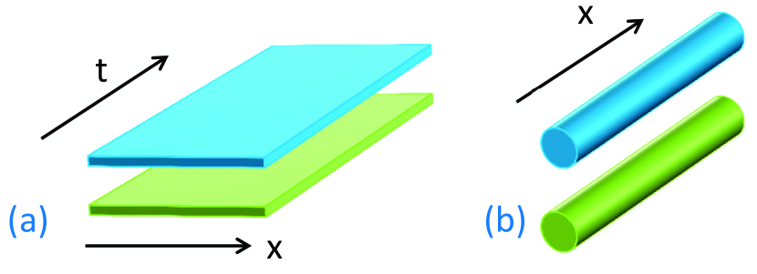
Figure 1: A schematic of ${\cal PT}$-symmetric coupled waveguides with gain (top waveguide) and loss (bottom waveguide). (a) Two waveguides on the plane where $t$ denotes the logitudinal and $x$ the transversal spatial coordinate. The transverse $x$-profiles of the stationary light beams evolve as they extend in the $t$ direction. (b) A pair of one-dimensional waveguides where light pulses undergo temporal evolution as they travel along the $x$ axis.

The paper is organized as follows. In the next section (Sec. II) we formulate the mathematical model and identify physically meaningful integral characteristics of the associated evolution. Two families of high- and low-frequency bright soliton solutions of the model are introduced in Sec. III. In the following section, Sec. IV, we outline the general framework for their stability analysis. The stability eigenvalues of the high-frequency soliton are classified in section V; there, we also follow the nonlinear evolution of instability when the soliton is found to be unstable. Section VI contains a similar study of the low-frequency soliton. Finally, section VII summarises conclusions of our work while three Appendices detail mathematical analyses of the stability eigenvalues.

II The model

To describe the dynamics of stationary light beams and pulses in coupled waveguides illustrated in Fig. 1, we extend the equations of the nonlinear $\mathcal{PT}$-symmetric coupler Chen et al. (1992); Ramezani et al. (2010); Sukhorukov et al. (2010). In the physical setting of Fig. 1(a), our extension takes into account the diffraction of the beam while in the situation represented by Fig. 1(b), we extend the system to include the effect of the pulse dispersion. The resulting equations have the following dimensionless form:

$$iu_{t}+u_{xx}+2|u|^{2}u=-v+i\gamma u,$$

$$iv_{t}+v_{xx}+2|v|^{2}v=-u-i\gamma v.$$ (1)

We note that this model was originally introduced as the continuous limit for a one-dimensional array of $\cal{PT}$-symmetric coupled waveguides Suchkov et al. (2011).

In Eqs.(1), the $u$ and $v$ variables are the normalized complex mode amplitudes in the top and bottom waveguides of Fig. 1. Considering stationary beams in the planar geometry of Fig. 1(a), the $t$ variable is the (spatial) coordinate in the propagation direction while $x$ is the transversal coordinate. In the temporal pulse interpretation [Fig. 1(b)], $t$ stands for time and $x$ for the spatial coordinate in the frame moving with the pulse group velocity. Here we assume that the group velocities and second-order dispersions in the waveguides are matched so as to satisfy the $\mathcal{PT}$-symmetry condition. By scaling the $x$ variable properly, we have normalized the coefficients in front of $u_{xx}$ and $v_{xx}$ terms to unity. (These terms account for the diffraction of spatial beams and dispersion of temporal pulses.)

We assume that the Kerr nonlinearity coefficients in the two waveguides (coefficients in front of $|u|^{2}u$ and $|v|^{2}v$) have the same value as this is necessary for the existence of solitons Suchkov et al. (2011). (These coefficients have been normalized to $2$ by scaling the mode amplitudes.) To ensure the existence of bright solitons, we take equal signs in front of the diffraction/dispersion and nonlinear terms. This corresponds to the self-focusing nonlinearity in the case of beams [Fig. 1(a)], and to the anomalous dispersion with positive Kerr nonlinearity or normal dispersion with negative nonlinearity — in the case of pulses [Fig. 1(b)].

Whether Eqs.(1) are employed to describe the stationary planar beams or temporal pulses, the first terms in the right-hand sides of (1) account for the coupling between the modes propagating in the two waveguides. The $\gamma$-terms describe the gain in one and loss in the other waveguide. Without loss of generality $\gamma$ can be taken positive; this choice corresponds to the gain in the top and loss in the bottom waveguide. The gain and loss coefficients are taken equal to conform to the $\mathcal{PT}$-symmetry condition Ruter et al. (2010).

We close this section by noting several physically meaningful quantities which prove useful in the understanding of the dynamics described by Eqs.(1). The first pair of variables give the powers associated with the $u$ and $v$ fields, respectively:

$$\mathcal{P}_{u}=\int|u|^{2}dx,\quad\mathcal{P}_{v}=\int|v|^{2}dx.$$ (2)

Neither individual powers nor their sum are conserved if $\gamma\neq 0$; however, the rate of change of the total power has a simple and insightful expression:

$$\frac{d}{dt}(\mathcal{P}_{u}+\mathcal{P}_{v})=2\gamma(\mathcal{P}_{u}-\mathcal{P}_{v}).$$ (3)

The momenta carried by the $u$ and $v$ components,

$$\mathcal{M}_{u}=\frac{i}{2}\int(u_{x}^{*}u-u_{x}u^{*})dx,\quad\mathcal{M}_{v}=\frac{i}{2}\int(v_{x}^{*}v-v_{x}v^{*})dx,$$ (4)

are not conserved either. The total momentum satisfies

$$\frac{d}{dt}({\mathcal{M}}_{u}+{\mathcal{M}}_{u})=2\gamma({\mathcal{M}}_{u}-{\mathcal{M}}_{v}).$$ (5)

Finally we note the rate equation

$$\frac{d\mathcal{H}}{dt}=2\gamma(\mathcal{R}_{u}-\mathcal{R}_{v}),$$ (6)

where

$$\mathcal{H}=\int\left[|u_{x}|^{2}+|v_{x}|^{2}-(|u|^{4}+|v|^{4})-(vu^{*}+v^{*}u)\right]dx$$ (7)

and

$$\mathcal{R}_{u}=\int(|u_{x}|^{2}-2|u|^{4})dx,\quad\mathcal{R}_{v}=\int(|v_{x}|^{2}-2|v|^{4})dx.$$ (8)

The integral $\mathcal{H}$ plays the role of the Hamiltonian of Eqs.(1) in the situation where there is no loss or gain ($\gamma=0$).

An immediate consequence of Eqs.(3), (5) and (6) is that all stationary states in the system (1) have to display symmetry between their two components: $\mathcal{P}_{u}=\mathcal{P}_{v}$, $\mathcal{M}_{u}=\mathcal{M}_{v}$, $\mathcal{R}_{u}=\mathcal{R}_{v}$.

III Solitons

Proceeding to the analysis of solutions to the system (1), it is convenient to make a change of variables

$$u(x,t)=e^{i(\Omega t-\theta)}U(x,t),\quad v(x,t)=e^{i\Omega t}V(x,t),$$ (9)

where $\theta$ is a constant angle satisfying

$$\sin\theta=\gamma,$$ (10)

and $\Omega$ is an arbitrary real parameter which will be conveniently chosen later. The transformation (9) casts equations (1) in the form

$$iU_{t}+U_{xx}-\Omega U+2|U|^{2}U=-\cos{\theta}\,V+i\gamma(U-V),$$

$$iV_{t}+V_{xx}-\Omega V+2|V|^{2}V=-\cos{\theta}\,U+i\gamma(U-V).$$ (11)

The system (11) admits an obvious reduction $U=V\equiv\phi$ to the scalar cubic Schrödinger equation,

$$i\phi_{t}+\phi_{xx}-a^{2}\phi+2|\phi|^{2}\phi=0,$$ (12)

where $a^{2}=\Omega-\cos\theta$. The relation (10) defines two different angles, $\theta=\arcsin\gamma$ and $\theta=\pi-\arcsin\gamma$. Accordingly, Eq.(12) describes two separate invariant manifolds of the system (1). Both invariant manifolds are characterised by the Hamiltonian evolution.

Equation (12) has a family of stationary soliton solutions. Without loss of generality we can restrict ourselves to time-independent solutions,

$$\phi(x)=a\,\mathrm{sech}(ax).$$

These define two coexisting families of stationary solitons of the original system (1), with arbitrary amplitudes $a>0$ and the corresponding frequencies

$$\Omega=a^{2}+\cos\theta.$$

The two families of solitons are distinguished by the sign of $\cos\theta$. One has $\cos\theta=\sqrt{1-\gamma^{2}}>0$; we will be denoting the corresponding solitons by ${\vec{\psi}}_{+}=(u_{+},v_{+})$. The other one [denoted ${\vec{\psi}}_{-}=(u_{-},v_{-})$ in what follows] has $\cos\theta=-\sqrt{1-\gamma^{2}}<0$. Note that for the given amplitude $a$, the frequency $\Omega$ corresponding to the soliton ${\vec{\psi}}_{+}$ is higher than that for ${\vec{\psi}}_{-}$. For this reason, we will be referring to the two solitons as ‘high frequency’ and ‘low frequency’ solitons. (It is fitting to note that the previous authors Suchkov et al. (2011) considered the high-frequency soliton only.)

We note that either family exists only if

$$\gamma<1.$$ (13)

At the same time, Eq.(13) gives the stability condition for the background solution $u=v=0$. In what follows, we will assume that (13) is always imposed.

IV Stability framework

IV.1 Perturbation decomposition

To classify the stability of the two families of solitons, we let

$$U(x,t)=\phi(x)+\delta U(x,t),\quad V(x,t)=\phi(x)+\delta V(x,t)$$ (14)

and linearise Eqs.(11) in $\delta U$ and $\delta V$. As we will see, a special role is played by the symmetric and antisymmetric combinations

$$p=\frac{\delta U+\delta V}{\sqrt{2}},\quad q=\frac{\delta U-\delta V}{\sqrt{2}}.$$ (15)

Since the linearised equations are autonomous in time, it is sufficient to consider separable solutions of the form

$$p=e^{\nu t}[(p_{1}^{\prime}+ip_{2}^{\prime})\cos\omega t+(p_{1}^{\prime\prime}+ip_{2}^{\prime\prime})\sin\omega t]$$

$$q=e^{\nu t}[(q_{1}^{\prime}+iq_{2}^{\prime})\cos\omega t+(q_{1}^{\prime\prime}+iq_{2}^{\prime\prime})\sin\omega t],$$ (16)

where we have introduced real components of four complex functions $p_{1}(x)$, $p_{2}(x)$, $q_{1}(x)$ and $q_{2}(x)$:

$$p_{1}=p_{1}^{\prime}+ip_{1}^{\prime\prime},\quad p_{2}=p_{2}^{\prime}+ip_{2}^{\prime\prime},$$

$$q_{1}=q_{1}^{\prime}+iq_{1}^{\prime\prime},\quad q_{2}=q_{2}^{\prime}+iq_{2}^{\prime\prime}.$$

In (16), both $\nu$ and $\omega$ are assumed to be real.

Substituting (16) in the linearised equations yields an eigenvalue problem

$$(\mathcal{L}-\cos\theta){\vec{p}}+2\gamma J{\vec{q}}=\mu J{\vec{p}},$$ (17a)

$$(\mathcal{L}+\cos\theta){\vec{q}}=\mu J{\vec{q}}$$ (17b)

for two-component complex vectors

$${\vec{p}}=\left(\begin{array}[]{c}p_{1}\\ p_{2}\end{array}\right),\quad{\vec{q}}=\left(\begin{array}[]{c}q_{1}\\ q_{2}\end{array}\right).$$

In (17a)-(17b) we have defined $\mu=\nu-i\omega$ and introduced the operator

$$\mathcal{L}=\left(\begin{array}[]{cc}-d^{2}/dx^{2}+\Omega-6\phi^{2}&0\\ 0&-d^{2}/dx^{2}+\Omega-2\phi^{2}\end{array}\right).$$

The $J$ in the right-hand sides of (17a)-(17b) stands for a skew-symmetric matrix:

$$J=\left(\begin{array}[]{lr}0&-1\\ 1&0\end{array}\right).$$

The rotation (15) did not diagonalise the $2\times 2$ block supermatrix in the left-hand side of (17); however it brought it to the triangular form. The triangular block matrix

$$\left(\begin{array}[]{cc}\mathcal{L}-\cos\theta&2\gamma J\\ 0&\mathcal{L}+\cos\theta\end{array}\right)$$ (18)

has two eigenvectors. One is

$$\left(\begin{array}[]{c}{\vec{p}}\\ 0\end{array}\right),$$ (19)

with ${\vec{p}}$ satisfying

$$(\mathcal{L}-\cos\theta){\vec{p}}=\mu J{\vec{p}}.$$ (20)

This is nothing but the linearised eigenvalue problem for the unperturbed cubic Schrödinger equation (the integrable nonlinear Schrödinger equation). (Thus ${\vec{p}}$ is the component of the perturbation that lies in the tangent space to the conservative manifold containing the soliton.) The spectrum of $\mu$ consists of a four-fold zero eigenvalue and the continuous spectrum which lies on the imaginary axis; there are no unstable $\mu$’s here.

The second eigenvector,

$$\left(\begin{array}[]{c}{\vec{p}}\\ {\vec{q}}\end{array}\right),$$ (21)

includes a nonzero ${\vec{q}}$ component. These $\vec{q}$ arise as eigenfunctions of the operator (17b). When $\vec{q}\neq 0$, Eq.(17a) becomes a nonhomogeneous equation with the right-hand side determined by ${\vec{q}}$:

$$\mathfrak{N}{\vec{p}}=-2\gamma J{\vec{q}}.$$ (22)

Here $\mathfrak{N}$ is a nonsymmetric operator defined by

$$\mathfrak{N}=\mathcal{L}-\cos\theta-\mu J.$$

As discussed in the previous paragraph, the eigenvalue problem (20) does not have nonzero eigenvalues; hence the adjoint operator

$$\mathfrak{N}^{\dagger}=\mathcal{L}-\cos\theta+\mu J$$

has null eigenvectors only if $\mu=0$. Therefore, for any $\mu\neq 0$, Eq.(22) has a bounded solution.

Thus the stability analysis reduces to solving the eigenvalue problem (17b). It is important to emphasise that, despite the presence of gain and loss, the eigenvalue problems (17b) and (20) are symplectic (that is, pertaining to Hamiltonian evolutions). The implication is that stable limit cycles are not the objects that can be expected to bifurcate from stationary solitons when the latter lose their stability. That is, the instability should evolve according to scenarios that are characteristic for conservative systems, e.g. breakup into long-lived transient structures, singular growth etc.

It is also worth commenting on the significance of the triangular representation (17) which decomposes small perturbations into the part tangent to the conservative invariant manifold containing the soliton, and the part that is transversal to this manifold. This decomposition alone explains some numerical observations of the previous authors Suchkov et al. (2011), in particular the instability of the bond-centred solitons in the discrete case. Indeed, the instability of the bond-centred soliton solutions of the discretised Eq.(1) is caused by perturbations lying in the conservative invariant manifold (that is, satisfying the scalar nonlinear Schrödinger equation). The instability of the bond-centred vector solitons is simply inherited from the instability of their scalar counterparts.

IV.2 Integral considerations

It is instructive to consider the effect of the perturbations on the Hamiltonian, momenta and the power integrals. Substituting Eqs.(14)-(16) in (2), (4) and (8), the right-hand sides of (3), (5) and (6) are evaluated to be

$$\left.(\mathcal{P}_{u}-\mathcal{P}_{v})\right|_{t=0}=2\sqrt{2}\int q_{1}^{\prime}(x)\phi(x)dx,$$ (23a)

$$\left.({\mathcal{M}}_{u}-{\mathcal{M}}_{v})\right|_{t=0}=-2\sqrt{2}\int q_{2}^{\prime}(x)\phi_{x}dx,$$ (23b)

$$\left.({\mathcal{R}}_{u}-{\mathcal{R}}_{v})\right|_{t=0}=-2\sqrt{2}\int\!q_{1}^{\prime}(x)(a^{2}+2\phi^{2})\phi\,dx.$$ (23c)

In Eqs.(23) we kept terms only up to the linear order in $p_{1,2}$ and $q_{1,2}$.

The eigenvector (19) has $q_{1}^{\prime}=q_{2}^{\prime}=0$; the corresponding rates (23) are all zero. The perturbations associated with eigenvectors of this type do not trigger the growth or decay of the total power, momentum and the Hamiltonian. They just take the soliton to a nearby solution of the scalar Schrödinger equation (12); the $\mathcal{PT}$ symmetry (the symmetry between the $u$ and $v$ components) remains unbroken.

As for the eigenvectors of the second type, Eqs.(21) with nonzero ${\vec{q}}$ and $\vec{p}$ satisfying (17b) and (22), they may set nonvanishing rates of change of the total power, momentum and Hamiltonian. Whether the right-hand side of Eq.(3), (5) or (6) is zero or not, depends, in particular, on the parity of the eigenfunction ${\vec{q}}(x)$ of the symplectic operator in (17b). If $({\vec{p}},{\vec{q}})^{T}$ is an eigenvector associated with an unstable eigenvalue ($\mathrm{Re}\,\mu>0$) and such that a particular right-hand side in Eq.(3), (5) or (6) is nonzero, the corresponding integral in the left-hand side will start evolving away from its soliton value.

In what follows, the perturbations of the integrals pertaining to the individual $u$ and $v$ components will also prove useful. Restricting ourselves to perturbations associated with real eigenvalues $\mu>0$, and substituting Eqs.(14)-(16) in (3) and (5), we arrive at

$$\delta{\mathcal{P}}_{u}=\sqrt{2}\left(\frac{2\gamma}{\mu}+1\right)e^{\mu t}\int q_{1}^{\prime}\phi\,dx,$$ (24a)

$$\delta{\mathcal{P}}_{v}=\sqrt{2}\left(\frac{2\gamma}{\mu}-1\right)e^{\mu t}\int q_{1}^{\prime}\phi\,dx,$$ (24b)

and

$${\mathcal{M}}_{u}=-\sqrt{2}\left(\frac{2\gamma}{\mu}+1\right)e^{\mu t}\int q_{2}^{\prime}\phi_{x}dx,$$ (25a)

$${\mathcal{M}}_{v}=-\sqrt{2}\left(\frac{2\gamma}{\mu}-1\right)e^{\mu t}\int q_{2}^{\prime}\phi_{x}dx.$$ (25b)

IV.3 Symplectic eigenvalue problem

Defining $X=ax$, $\lambda=\mu/a^{2}$, and introducing

$$\eta=2\frac{\cos\theta}{a^{2}},$$ (26)

the problem (17b) can be written as

$$\left(\begin{array}[]{cc}L_{1}+\eta&0\\ 0&L_{0}+\eta\end{array}\right)\left(\begin{array}[]{c}g\\ f\end{array}\right)=\lambda J\left(\begin{array}[]{c}g\\ f\end{array}\right).$$ (27)

Here $L_{0,1}$ stand for the scalar Sturm-Liouville operators

$$L_{0}=-d^{2}/dX^{2}+1-2\,\mathrm{sech}^{2}X,$$

$$L_{1}=-d^{2}/dX^{2}+1-6\,\mathrm{sech}^{2}X,$$ (28)

and we have redenoted $q_{1}=g$ and $q_{2}=f$ for notational convenience. The eigenvalues $\lambda$ and eigenvectors $(g,f)$ are generally complex. Positive $\eta$ correspond to the soliton ${\vec{\psi}}_{+}$ and negative to ${\vec{\psi}}_{-}$.

Thus we have reduced a two-parameter stability problem to an eigenvalue problem involving a single similarity parameter. Solitons with different amplitudes and in systems with different gain-loss coefficients have the same stability properties as long as they share the value of $\eta$. (It is fitting to note that a self-similarity of this sort was previously encountered in the parametrically driven damped nonlinear Schrödinger equation Barashenkov et al. (1991, 2002). The difference of the parametrically driven situation from the present setting was that there, the similarity combination included two control parameters of the equation whereas Eq.(26) combines a control parameter with a free amplitude of the soliton.)

The scalar operators have familiar spectral properties. The only discrete eigenvalue of $L_{0}$ is zero; the associated eigenfunction is even: $L_{0}z_{0}=0$, $z_{0}=\,\mathrm{sech}X$. The operator does not have other eigenvalues between 0 and 1 (the edge of the continuous spectrum). The lowest eigenvalue of $L_{1}$ is $-3$; the associated eigenfunction is $y_{0}=\,\mathrm{sech}^{2}X$. The only other eigenvalue is 0; the corresponding eigenfunction $y_{1}=\,\mathrm{sech}X\tanh X$ is odd.

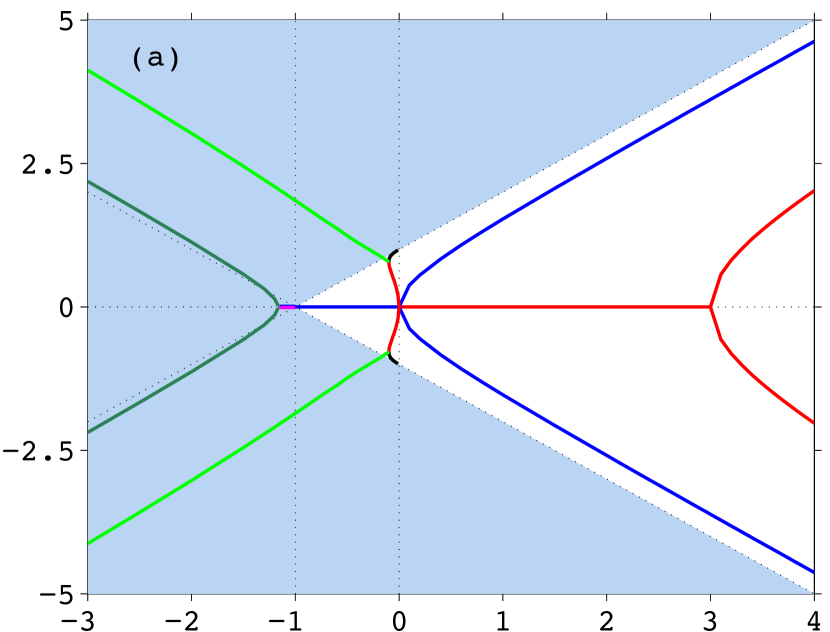
Figure 2: (a) the imaginary and (b) real part of the eigenvalue $\lambda$ of the problem (27) as a function of ${\eta}$. (For the fixed $\gamma$, the parameter $\eta$ is proportional to the inverse amplitude squared: $\eta=2\cos\theta/a^{2}$.) A real pair of eigenvalues moves onto the imaginary axis while the imaginary pair becomes real as ${\eta}$ passes through zero (either way). In the ${\eta}>0$ part of the figure, the real pair subsequently converges and returns to the imaginary axis, so that for ${\eta}\geq 3$, all eigenvalues are pure imaginary. In the ${\eta}<0$ part, two complex quadruplets are born in two consecutive Hamiltonian Hopf bifurcations. The imaginary parts of the quadruplets grow as ${\eta}\to-\infty$ while the real parts decay. In (a), tinted are the regions $\mathrm{Im}\,\lambda\geq\eta+1$ and $\mathrm{Im}\,\lambda\leq-(\eta+1)$ filled with the continuous spectrum.

When $\eta=0$, the eigenvalue problem (27) coincides with the eigenvalue problem for the unperturbed cubic nonlinear Schrödinger equation. It is important to emphasise, however, that the choice ${\eta}=0$ does not correspond to the undamped-undriven situation. (The undamped-undriven limit $\gamma=0$ does not single out any particular ${\eta}$ and is not special in any way.) What the value ${\eta}=0$ corresponds to, is the turning point $\gamma=1$. As $\gamma$ reaches 1 from below, the solitons ${\vec{\psi}}_{+}$ and ${\vec{\psi}}_{-}$ merge and disappear.

As in the unperturbed nonlinear Schrödinger, there is a four-fold zero eigenvalue at the point ${\eta}=0$: $\lambda^{(1,2,3,4)}=0$. As ${\eta}$ deviates from zero, the four eigenvalues move out of the origin. A pertubation calculation (Appendix A) shows that two opposite eigenvalues move on to the imaginary axis, and the other two move on to the positive and negative real axis, respectively:

$$\lambda^{(1,2)}=\pm 2{\eta}^{1/2}+O({\eta}),\quad\lambda^{(3,4)}=\pm\frac{2}{\sqrt{3}}(-\eta)^{1/2}+O(\eta).$$ (29)

The real and imaginary parts of eigenvalues of the problem (27), obtained numerically, are plotted in fig.2. The two pairs of real and imaginary eigenvalues emerging from the origin, are clearly visible.

Before proceeding to the evolution of the eigenvalues as ${\eta}$ grows to large positive respectively negative values, it is appropriate to note the position of the continuous spectrum the symplectic operator

$$J^{-1}\left(\begin{array}[]{cc}L_{1}+{\eta}&0\\ 0&L_{0}+{\eta}\end{array}\right)$$ (30)

in (27). There are two branches of continuous spectrum, both lying on the imaginary axis of $\lambda$: $\lambda=\pm i\omega(k)$, where $\omega=1+{\eta}+k^{2}$. (These are indicated by shading in fig.2(a).) When ${\eta}>-1$, the continuous spectrum has a gap, $[-i(1+{\eta}),i(1+{\eta})]$.

It is also worth mentioning that the spectrum of symplectic operators consists of pairs of opposite pure-imaginary values, real pairs and complex quadruplets. If $\lambda$ is a real or pure imaginary point of the spectrum, then $-\lambda$ is another one; if a complex $\lambda$ is in the spectrum, then so are $-\lambda,\lambda^{*}$, and $-\lambda^{*}$ Arnold (2010).

V High frequency soliton

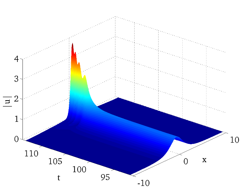
Figure 3: The evolution of the perturbed soliton ${\vec{\psi}}_{+}$ with the amplitude $a$ above the threshold $a_{c}$. Shown is the magnitude of the field $u$ (a) and field $v$ (b). The control parameter is set to $\gamma=0.1$ (for which $a_{c}=0.814$); the soliton’s amplitude is $a=0.820$. Note that the spatial interval has been cut down to $(-10,10)$ for visual clarity and that only the late stage of evolution is shown. In both panels the colour varies from deep blue (lowest elevation) to deep red (highest elevation); since the maximum values of $|u|$ and $|v|$ are not equal, the same colour corresponds to different values in the two panels. The same convention is used in all other double-panel 3D plots.

Figure 4: The evolution of the unstable soliton ${\vec{\psi}}_{+}$ may result in the formation of a breather. Shown is the magnitude of the field $u$ (a) and field $v$ (b). Here $\gamma=0.1$ and $a=0.9$.

In the case of the soliton ${\vec{\psi}}_{+}$, the eigenvalue problem is amenable to simple analysis. The lowest eigenvalue of the operator $L_{0}+\eta$ equals ${\eta}$; therefore, when ${\eta}>0$, the operator $L_{0}+{\eta}$ is positive definite and admits an inverse. The problem (27) can be written then as a generalised eigenvalue problem for a scalar function $g(X)$:

$$(L_{1}+{\eta})g=-\lambda^{2}(L_{0}+{\eta})^{-1}g.$$ (31)

The operator on the left in (31) is symmetric, and the one on the right is symmetric and positive definite. The lowest eigenvalue $-\lambda^{2}$ in (31) is given by the minimum of the Rayleigh quotient:

$$-\lambda^{2}=\min\frac{\langle g|L_{1}+{\eta}|g\rangle}{\langle g|(L_{0}+{\eta})^{-1}|g\rangle}.$$ (32)

[Here the bra-ket notation is used for the $\mathcal{L}^{2}$ scalar product: $\langle y|z\rangle=\int y(X)z(X)dX$.] The minimum is positive if the lowest eigenvalue of the operator in the numerator ($\nu=-3+{\eta}$) is positive: ${\eta}>3$. Recalling the definition (26), we arrive at the stability condition for the soliton ${\vec{\psi}}_{+}$:

$$a\leq a_{c},\quad a_{c}^{2}=\frac{2}{3}\sqrt{1-\gamma^{2}}.$$ (33)

Figure 5: Chart of asymptotic regimes emerging from the unstable soliton ${\vec{\psi}}_{+}$. The five columns correspond to $\gamma=0.1,0.2,0.5,0.7$ and $0.95$. The solid line demarcates the boundary (33); the ${\vec{\psi}}_{+}$ soliton is unstable above this line. The magenta triangles mark blowups while green circles indicate the formation of breathers.

The numerical study of the eigenvalue problem (27) corroborates these conclusions. As ${\eta}$ grows from 0 to positive values, two pairs of opposite eigenvalues, a real and a pure imaginary pair, appear from the origin on the $(\mathrm{Re}\,\lambda,\mathrm{Im}\,\lambda)$ plane. The real eigenvalues are associated with even and imaginary pair with odd eigenfunctions. The two pure imaginary eigenvalues diverge to their respective infinities (fig.2(a)). The real pair first grows in absolute value, but then the real eigenvalues reverse (fig.2(b)) and, as ${\eta}$ reaches $3$, collide at the origin and move on to the imaginary axis. The emerging second pair of imaginary eigenvalues diverges to the infinities, like the first pair before (fig.2(a)).

The quantity $q(X,t)$ in (15) measures the difference between the two components of the vector $(U,V)$. If the eigenvalue problem (27) has a positive eigenvalue $\lambda$, the difference grows monotonically: $q=(q_{1}+iq_{2})e^{\lambda a^{2}t}$. Therefore, the instability associated with real eigenvalues should manifest itself as a monotonically growing asymmetry between the two components of the vector field. Quantitatively, this asymmetry is measured by the difference in the increments of the ${\mathcal{P}}_{u}$ and ${\mathcal{P}}_{v}$ integrals, Eqs.(24).

Transient and asymptotic solutions emerging as the perturbation grows, should inherit the spatial parity of the eigenvector $(g(X),f(X))$ associated with the real eigenvalue — that is, should be even in $X$.

The imaginary eigenvalues correspond to internal modes of the soliton. In Appendix B, we derive the asymptotes for both pairs of imaginary eigenvalues as ${\eta}\to\infty$: $\lambda=\pm i(\eta+0.685)+O(1/\eta)$ and $\lambda=\pm i(\eta-~{}1.438)+O(1/\eta)$.

Figs 3 and 4 present results of direct numerical simulations of the ${\vec{\psi}}_{+}$ soliton. For five values of the control parameter, $\gamma=0.1$, $0.2$, $0.5$, $0.7$, and $0.95$, we simulated solitons with amplitudes $a$ above the critical one, $a_{c}$, given by (33). In each of the five cases we have identified two possible scenarios of instability growth. In one of these, the magnitude of the field $u$ grows without bound, while $v$ decreases. (See fig.3.) We will be referring to this type of evolution as the ‘blowup’. Note that this asymmetry-growth scenario is in agreement with our expectations based on the eigenfunction analysis.

In the other scenario, the breakup of the unstable soliton results in the formation of a long-lived oscillatory state — a kind of a breather (fig. 4). Here, the initial stage of the evolution is also characterised by the growth of asymmetry. Unlike fig.3, it is the $v$ component that is growing this time, and $u$ is the one that is decreasing (clearly visible in fig. 4). This “anomalous” growth cannot continue indefinitely [this would contradict Eq.(3)] and eventually the evolution is captured into the breather regime.

Fig.5 sketches the ranges of $a$ which are characterised by each of these two types of instability growth. Typically, solitons with amplitudes only slightly exceeding the threshold (33) give rise to breathers whereas the blow-up scenario is observed for larger $a$. The exception from this rule occurs for small $\gamma\sim 0.1$ where the blowup and breather domains seem to be interlaced in a more complex fashion.

VI Low frequency soliton

When ${\eta}<0$, neither of the scalar operators in (27) is invertible on the $\mathcal{L}^{2}$ space. Here, the analysis of the eigenvalue problem (27) has to be done mostly by numerical means. Our numerical study is summarised in the left half of fig.2.

As ${\eta}$ is decreased through zero, a pair of opposite real eigenvalues (associated with even eigenfunctions) collides and moves on to the imaginary axis. Simultaneously (that is, at ${\eta}=0$) another pair of opposite imaginary eigenvalues (also with even eigenfunctions) detaches from the continuous spectrum. When ${\eta}$ reaches the value $\eta_{1}$,

$$\eta_{1}=-0.0988,$$ (34)

the four imaginary eigenvalues collide, pairwise, and leave the imaginary axis forming a complex quadruplet $\lambda,\lambda^{*},-\lambda,-\lambda^{*}$ (with even eigenfunctions). As ${\eta}$ grows to larger negative values, the real parts of the quadruplet first grow but then start decreasing. At the same time, the imaginary parts grow without bound.

Another pair of eigenvalues colliding as ${\eta}$ is decreased through zero, is pure imaginary. Unlike the colliding real pair, the imaginary pair is associated with odd eigenfunctions. The parity of the eigenfunctions is preserved as this pair reappears on the real axis for ${\eta}<0$. As ${\eta}$ grows to larger negative values, the absolute values of the real $\lambda$ first grow but then start decreasing.

The existence of the real pair in the interval $-1<{\eta}<0$ can be established analytically. (See Appendix C.) It might be tempting to expect the pair to converge at the origin as ${\eta}$ reaches $-1$; however the actual bifurcation diagram turns out to be more complex (fig.2). In fact one can prove that $\mathrm{Re}\ \lambda$ remains nonzero at ${\eta}=-1$. (See Appendix C.)

In the meantime, as ${\eta}$ is approaching $-1$, the gap in the continuous spectrum is shrinking. As ${\eta}$ reaches $-1$, the two edges of the continuous spectrum meet at the origin and the gap closes. Due to the resonance between the edge eigenfunctions, a new pair of discrete eigenvalues is born at this point. Like the coexisting real pair, this pair of opposite real eigenvalues is associated with odd eigenfunctions. As ${\eta}$ drops down to $\eta_{2}$, where

$$\eta_{2}=-1.168,$$ (35)

the newly born pair of real eigenvalues and the real pair that has arrived from the origin collide and emerge into the complex plane. This is where the second complex quadruplet is born. As the negative ${\eta}$ continues to grow in absolute value, the real parts of the eigenvalues making up the quadruplet decrease, while the imaginary parts grow.

Thus when ${\eta}<\eta_{2}$, we have two complex quadruplets. As ${\eta}$ grows in absolute value, the real parts of the eigenvalues in both quadruplets decrease whereas imaginary parts grow. In the Appendix B we derive the asymptotic behaviour of the imaginary parts analytically: $\mathrm{Im}\,\lambda=\pm(\eta-1.438)+O(1/\eta)$; $\mathrm{Im}\,\lambda=\pm(\eta+0.685)+O(1/\eta)$. We also show that the decrease of the real parts is exponentially fast. Eq.(26) implies then that solitons with small amplitude $a$ — even if are unstable — have exponentially long lifetime,

$$\tau\sim\frac{1}{a^{2}}\exp\left(\frac{\sigma\sqrt{1-\gamma^{2}}}{a^{2}}\right),$$

with some constant $\sigma>0$.

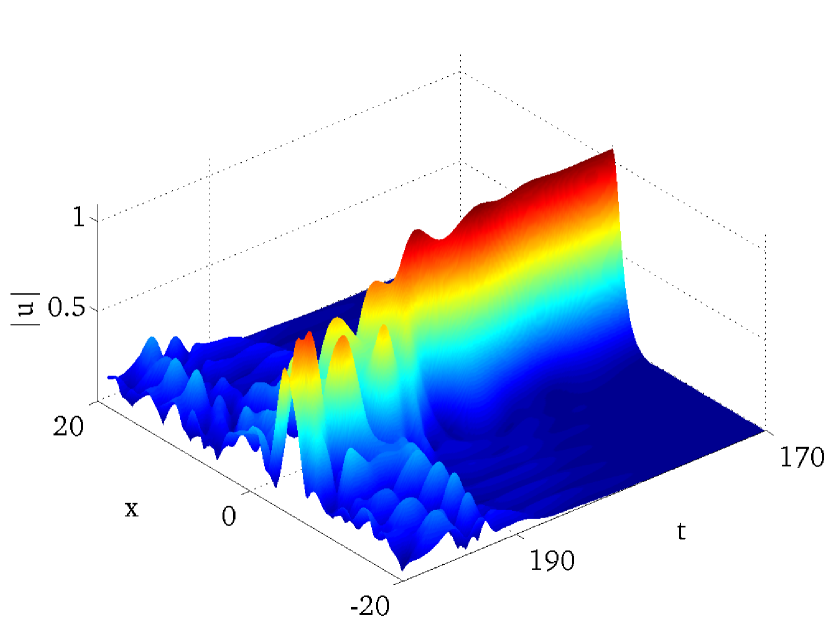
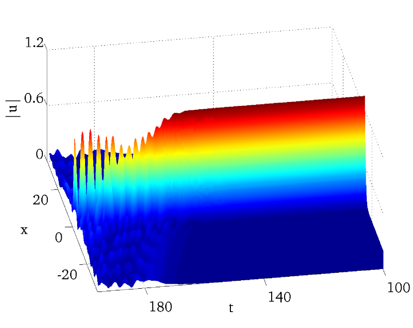
Figure 6: Unstable $\psi_{-}$ solitons with $|\eta|>1.168$ disperse (a) or transform into a long-lived breather (b). In (a), $\gamma=0.5$ and $a=1.075$; in (b), $\gamma=0.1$ and $a=1.152$. Both combinations of $a$ and $\gamma$ correspond to ${\eta}=-1.5$. Only the $u$-component is shown in both cases; the evolution of the $v$ field is qualitatively similar.

The nonlinear evolution of the unstable ${\vec{\psi}}_{-}$ soliton is determined by the competition between the eigenvalues with positive real parts. According to fig.2, there are two ranges of the soliton amplitude for each $\gamma$: the small and the large $a$.

For small $a$ [more precisely, for $a$ such that $|\eta|>|\eta_{2}|$ with $\eta_{2}$ as in (35)], the soliton has two complex quadruplets in its spectrum — one with an even and the other one with an odd eigenvector. Accordingly, the instability growth of a small-amplitude ${\vec{\psi}}_{-}$ soliton should be accompanied by oscillations. The growth rate of the odd perturbation is larger than that of the even one; therefore the generic evolution of the instability is expected to be dominated by the odd perturbations.

On the other hand, for very large $a$ — more precisely, for $\eta_{1}<\eta<0$, with $\eta_{1}$ as in (34) — the spectrum has only one, real, unstable eigenvalue (with an odd eigenvector). In this range, the instability growth should be initially monotonic. The moderately large amplitudes (corresponding to $\eta_{2}<\eta<\eta_{1}$) are characterised by one or two positive real eigenvalues, with odd eigenvector(s), and a complex quadruplet whose eigenvector is even in $X$. The odd eigenfunctions have larger growth rates than the even ones; hence again, the monotonically growing odd perturbations should be dominating the evolution.

Thus, depending on the soliton’s amplitude, the odd perturbations are either the only unstable perturbations of the ${\vec{\psi}}_{-}$ soliton, or its dominant unstable perturbations. For these, Eqs.(24) give $\delta{\mathcal{P}}_{u}=\delta{\mathcal{P}}_{v}=0$. Therefore, the odd perturbations do not immediately induce the asymmetry of the $u$ and $v$ components of the soliton. On the other hand, the momenta ${\mathcal{M}}_{u}$ and ${\mathcal{M}}_{v}$ in Eqs.(25) are both nonzero, with ${\mathcal{M}}_{u}\neq{\mathcal{M}}_{v}$. This means that the two components, the “$u$ pulse” and the “$v$ pulse”, will be set in motion — they will start moving with unequal velocities gradually separating in space. As a result, the “$u$ pulse” will be progressively deprived of the services of its power-draining partner, while the “$v$ pulse” will be cut from the power supply by its active counterpart. Eventually, this will set off the growth of the asymmetry in the amplitudes of the pulses — the ${\mathcal{P}}_{u}$ will start growing and ${\mathcal{P}}_{v}$ decreasing.

Equations (25) can tell us whether the emerging pulses will move in the opposite or in the same direction (yet with different velocities). Indeed, the fragments will move in the opposite directions if the momenta (25) are opposite in signs: $2(\gamma/\mu)-1<0$. Recalling that $\mu=\lambda a^{2}$, this condition can be written as

$$a^{2}>\frac{2\gamma}{\lambda}.$$ (36)

In the complementary region, $a^{2}<2\gamma/\lambda$, the $u$- and $v$-pulses will move in the same direction.

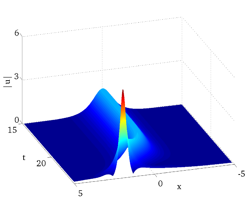
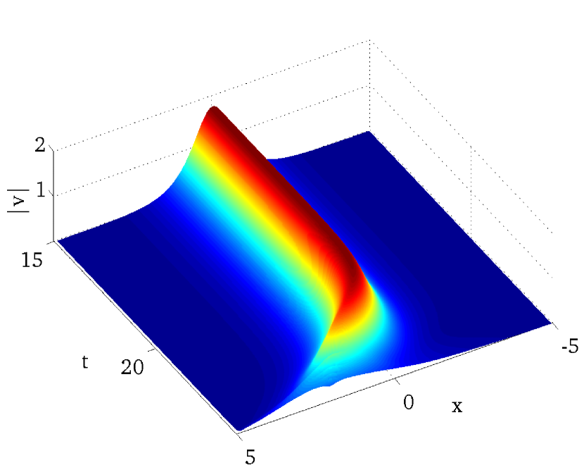
Figure 7: A spontaneous motion of the soliton ${\vec{\psi}}_{-}$ followed by the blowup of its $u$-component and decay of $v$. Here $\gamma=0.95$ and $a=1.767$ (${\eta}=-0.2$).

To verify these predictions, we carried out numerical simulations of solitons with a range of amplitudes, for small and large values of the gain-loss rate ($\gamma=0.1$, $0.2$, $0.5$, $0.7$, and $0.95$).

In agreement with the linear analysis, the small-amplitude ($|\eta|>|\eta_{2}|$) unstable solitons were detected either to disperse (a process accompanied by the oscillation of the soliton profiles, see fig.6(a)) or form long-lived oscillatory states (fig.6(b)).

The instability of solitons with large and moderately large amplitudes ($|\eta|<|\eta_{2}|$) was seen to grow monotonically, at least at the initial stage. One of the recorded scenarios starts with a spontaneous motion of the two components of the soliton in the same direction, with slightly different velocities (fig.7), followed by the blowup of the $u$-component and decay of its $v$ counterpart. This behaviour was detected for the amplitudes $a$ lying outside the region (36). (In particular, the unstable soliton shown in fig.7 has $a^{2}=3.12$ which is smaller than the value $2\gamma/\lambda=4.00$ corresponding to $\gamma=0.95$ and $\eta=-0.2$.)

The other observed evolution starts with the motion of the two components in opposite directions. In this case the dissociation of the ${\vec{\psi}}_{-}$ soliton may be followed by a blowup of $u$ and decay of $v$ (fig.8) or a formation of a pair of breathers (fig.9). Lastly, the linear instability may “just miss” the breathers’ basin of attraction in which case the nuclei of the two breathers will have their $u$ component blow up (fig.10). These types of evolution were recorded for the amplitudes $a$ satisfying the condition (36). (In particular, fig.8 corresponds to $a^{2}=9.92$ and $2\gamma/\lambda=0.42$; fig.9 to $a^{2}=2.84$ and $2\gamma/\lambda=0.31$; and fig.10 to $a^{2}=3.32$ and $2\gamma/\lambda=0.31$.)

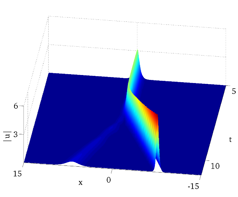
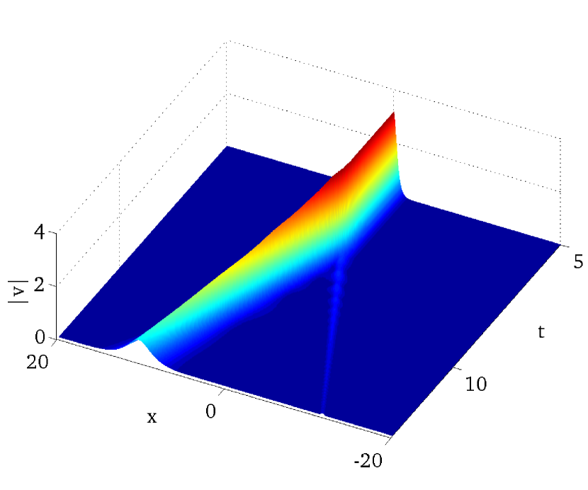
Figure 8: A dissociation of the soliton ${\vec{\psi}}_{-}$ into a pair of pulses followed by the blowup of the pulse with large $u$-component. Shown is the magnitude of the field $u$ (a) and field $v$ (b). Here $\gamma=0.1$ and $a=3.15$ (${\eta}=-0.2$).

Our numerical simulations of the unstable regimes are summarised in fig.11. Triangles mark parameter values for which the unstable soliton or the two fragments of its break-up were observed to blow up; circles indicate simulations that ended in the formation of one or two breathers. The solid curve in the figure is the demarcation line between the small- and large-amplitude ranges identified in the linear analysis; the curve is defined by $\eta=\eta_{2}$ with $\eta_{2}$ as in (35). The chart shows a clear correlation between the type of the unstable eigenvalues (real vs complex) and the soliton decay product (blowup vs breathers).

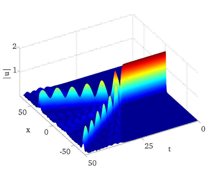
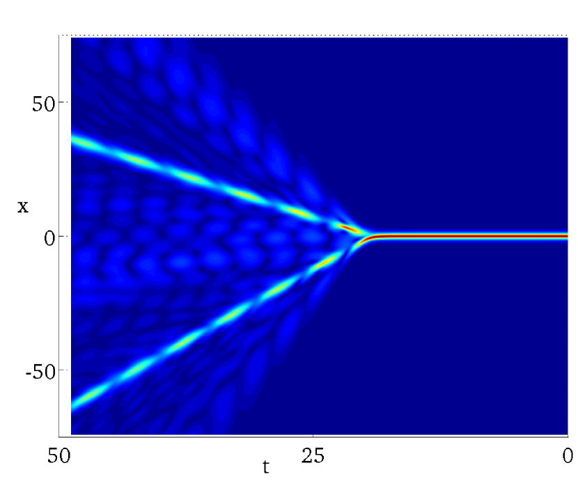
Figure 9: A dissociation of the soliton ${\vec{\psi}}_{-}$ into a pair of breathers. Shown is the magnitude of $u$ (a) and contour plot of $|v|$ (b). Here $\gamma=0.1$ and $a=1.686$ (${\eta}=-0.7$).

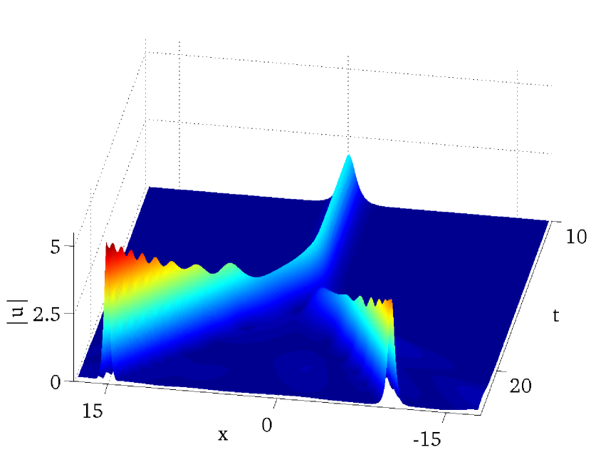
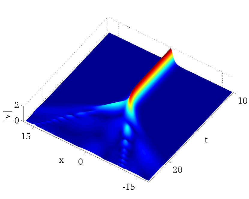
Figure 10: A dissociation of the soliton ${\vec{\psi}}_{-}$ into a pair of pulses followed by their blowup. Shown is the magnitude of $u$ (a) and modulus of $v$ (b). Here $\gamma=0.1$ and $a=1.8212$ ($\eta=-0.6$).

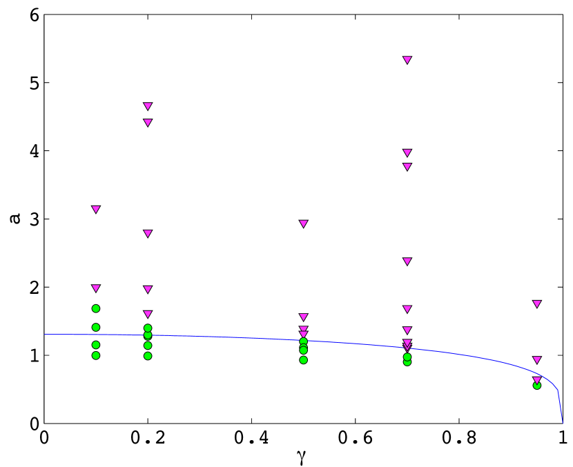
Figure 11: Chart of asymptotic regimes emerging from the unstable soliton ${\vec{\psi}}_{-}$. The solid curve is given by $a^{2}=(-2/\eta_{2})\sqrt{1-\gamma^{2}}$. The magenta triangles mark blowups while green circles indicate the bounded regimes: dispersion of the soliton or formation of breathers.

VII Conclusions

We have examined stability of two families of solitons in the two-dimensional $\mathcal{PT}$ symmetric coupler with gain and loss. The dynamical regimes set off by the instability have also been explored. The results of our study can be summarised as follows.

1. Despite the presence of gain and loss, the bifurcations occurring in the $\mathcal{PT}$-symmetric system (1) are of conservative type. (Linearised eigenvalues cross from the imaginary to the real axis, or collide, pairwise, on the imaginary axis and emerge into the complex plane.) As a result, the soliton instability cannot give rise to localised limit cycles (which would be a typical outcome of the Hopf bifurcation in a dissipative system). In the $\mathcal{PT}$-symmetric system, the soliton instability either triggers its blowup (the process where the amplitude grows without bound at an exponential rate) or produces finite-lifetime breathers.

2. The soliton stability and internal dynamics are determined by a single self-similar combination ($\eta$) of the gain-loss coefficient $\gamma$ and the soliton’s amplitude $a$.

3. The high-frequency solitons with amplitudes smaller than $a_{c}$, where $a_{c}$ is as in (33), are stable, and with amplitudes greater than $a_{c}$, unstable. All low-frequency solitons are unstable; however the lifetimes of the solitons with small amplitudes are exponentially long so for all practical purposes they can be regarded as stable.

4. The mechanisms of instability of the high- and low-frequency soliton are different. The unstable perturbation of the high-frequency soliton triggers the growth of asymmetry between the active ($u$) and lossy ($v$) components of the soliton, destroying the gain/loss balance in the system. The unstable perturbation of the low-frequency soliton also upsets the energy balance; however this time it is done by splitting the $u$ and $v$ components off from their common axis. The difference in the instability mechanisms is reflected in the difference in the products of the high- and low-frequency soliton breakup.

Appendix A Real-imaginary eigenvalue transitions

The aim of this Appendix is to describe the transitions of the pair of eigenvalues of the operator (27) from the real to imaginary axis and vice versa, as the parameter $\eta$ crosses through zero in either direction.

The numerical analysis indicates that when $\eta$ approaches 0, the eigenvalue scales as $\eta^{1/2}$. This suggests an expansion of the form

$$\lambda=\eta^{1/2}\lambda_{1}+\eta\lambda_{2}+...;$$

$$g=g_{0}+\eta^{1/2}g_{1}+\eta g_{2}+...,$$

$$f=f_{0}+\eta^{1/2}f_{1}+\eta f_{2}+....$$ (37)

This expansion will be validated if all coefficient functions are found to be bounded and decaying to zero as $X\to\pm\infty$.

The expansion (37) is similar to the one appearing in the parametrically driven damped nonlinear Schrödinger equation Barashenkov et al. (1991, 2002). The difference of Eq.(27) from the eigenvalue problem in Barashenkov et al. (1991, 2002), is that the parametric driving breaks only one of the invariances of the nonlinear Schrödinger (only the operator $L_{0}$ is perturbed). On the other hand, in Eq.(27), both $L_{0}$ and $L_{1}$ acquire perturbations. The consequence of this will be the motion of two pairs of eigenvalues through the origin on the $\lambda$ plane. While one pair is moving from the real to imaginary axis, the other pair will be moving in the opposite direction.

Substituting (37) in (27) and equating coefficients of like powers of $\eta$, we obtain a chain of equations for $\lambda_{n}$, $g_{n}$ and $f_{n}$. The order $\eta^{0}$ gives

$$L_{0}f_{0}=0,\quad L_{1}g_{0}=0.$$

These two equations coincide with equations for the $U(1)$ and translational zero modes of the scalar cubic nonlinear Schrödinger equation. The bounded solutions are

$$f_{0}=C_{1}\,\mathrm{sech}X,\quad g_{0}=C_{2}\,\mathrm{sech}X\tanh X,$$

where $C_{1}$ and $C_{2}$ are arbitrary constants.

At the next, $\eta^{1/2}$, order, we get a pair of nonhomogeneous equations

$$L_{0}f_{1}=\lambda_{1}g_{0},\quad L_{1}g_{1}=-\lambda_{1}f_{0},$$

whose solutions are

$$f_{1}=\frac{C_{2}}{2}\lambda_{1}X\,\mathrm{sech}X,\quad g_{1}=\frac{C_{1}}{2}\lambda_{1}\,\mathrm{sech}X(1-X\tanh X).$$

In the context of stability of the scalar cubic nonlinear Schrödinger soliton, the generalised eigenvectors $(0,f_{1})^{T}$ and $(g_{1},0)^{T}$ would correspond to the Galilean invariance of that equation and its soliton frequency variations.

Finally, the order $\eta^{1}$ gives

$$L_{0}f_{2}=-f_{0}+\lambda_{1}g_{1}+\lambda_{2}g_{0},$$ (38)

$$L_{1}g_{2}=-g_{0}-\lambda_{1}f_{1}-\lambda_{2}f_{0}.$$ (39)

The solvability condition for Eq.(38) is

$$-\langle z_{0}|f_{0}\rangle+\lambda_{1}\langle z_{0}|g_{1}\rangle=0,$$ (40)

and the one for (39) is

$$-\langle y_{1}|g_{0}\rangle-\lambda_{1}\langle y_{1}|f_{1}\rangle=0.$$ (41)

In (40)-(41), $z_{0}=\,\mathrm{sech}X$ and $y_{1}=\,\mathrm{sech}X\tanh X$ are the null eigenvectors of the operator $L_{0}$ and $L_{1}$, respectively. The bra-ket notation is used for the $\mathcal{L}^{2}$ scalar product:

$$\langle y|z\rangle=\int y(X)z(X)dX.$$

Substituting for $f_{0,1}$ and $g_{0,1}$ in (40)-(41), the solvability conditions reduce to

$$C_{1}\left(\frac{\lambda_{1}^{2}}{2}-2\right)=0,$$

$$C_{2}\left(\frac{\lambda_{1}^{2}}{2}+\frac{2}{3}\right)=0,$$

whence either $\lambda_{1}=\pm 2$ and $C_{2}=0$, or $\lambda_{1}=\pm 2i/\sqrt{3}$ and $C_{1}=0$.

This gives us the the leading-order expressions for the two pairs of eigenvalues and eigenvectors of the operator (27) with small $\eta$. One pair of eigenvalues is $\lambda=\pm 2\sqrt{\eta}+O(\eta)$; it is associated with even eigenfunctions:

$$\left(\begin{array}[]{c}g\\ f\end{array}\right)=\left(\begin{array}[]{c}\pm\sqrt{\eta}\,\mathrm{sech}X(1-X\tanh X)\\ \,\mathrm{sech}X\end{array}\right)+O(\eta).$$

This pair moves from the real to imaginary axis as $\eta$ decreases from positive to negative values.

The other pair of eigenvalues is $\lambda=\pm 2\sqrt{-\eta/3}+O(\eta)$. The corresponding eigenfunctions are odd:

$$\left(\begin{array}[]{c}g\\ f\end{array}\right)=\left(\begin{array}[]{c}\,\mathrm{sech}X\tanh X\\ \pm i\sqrt{\frac{\eta}{3}}X\,\mathrm{sech}X\end{array}\right)+O(\eta).$$

As $\eta$ moves from positive to negative, this pair of eigenvalues translates from the imaginary to real axis.

Appendix B Asymptotic eigenvalues as $|{\eta}|\to\infty$

In this Appendix, we determine the asymptotic behaviour of eigenvalues of the operator (27) as ${\eta}$ tends to $\pm\infty$.

We expand

$$f=f_{0}+\frac{f_{1}}{{\eta}}+\frac{f_{2}}{{\eta}^{2}}+...,$$

$$g=g_{0}+\frac{g_{1}}{{\eta}}+\frac{g_{2}}{{\eta}^{2}}+...;$$

$$\lambda=i\left(\lambda_{-1}{\eta}+\lambda_{0}+\frac{\lambda_{1}}{{\eta}}+\frac{\lambda_{2}}{{\eta}^{2}}+...\right).$$

It is convenient to introduce coefficient functions $\mathcal{A}_{n}(X)$ and $\mathcal{B}_{n}(X)$,

$$\mathcal{A}_{n}=f_{n}-ig_{n},\quad\mathcal{B}_{n}=-(f_{n}+ig_{n}).$$

Substituting in (27), and equating coefficients of ${\eta}^{-n}$, gives

$$\lambda_{-1}^{2}=1,\quad\mathcal{A}_{0}=0$$ (42)

at the order ${\eta}^{1}$, and

$$(L_{1/2}-\lambda_{0})\mathcal{B}_{n}=2\,\mathrm{sech}^{2}X\mathcal{A}_{n}+\sum_{m=1}^{n}\lambda_{m}\mathcal{B}_{n-m}$$ (43)

$$2\mathcal{A}_{n+1}=2\,\mathrm{sech}^{2}X\mathcal{B}_{n}-(L_{1/2}+\lambda_{0})\mathcal{A}_{n}-\sum_{m=1}^{n}\lambda_{m}\mathcal{A}_{n-m}$$ (44)

for all $n\geq 0$. Here we have introduced an operator

$$L_{1/2}=-d^{2}/dX^{2}+1-4\,\mathrm{sech}^{2}X.$$

In Eq.(42) we can choose, without loss of generality, $\lambda_{-1}=1$. [The other root, $\lambda_{-1}=-1$, defines the opposite eigenvalue, $-\lambda$, with the eigenvector $(g,-f)^{T}$.]

Equation (43) with $n=0$ is an eigenvalue problem for the operator $L_{1/2}$:

$$L_{1/2}\mathcal{B}_{0}(X)=\lambda_{0}\mathcal{B}_{0}(X).$$

The potential $-4\,\mathrm{sech}^{2}X$ is of the Pöschl-Teller variety so the eigenvalues can be found exactly. There are two discrete eigenvalues, $\rho_{A}$ and $\rho_{B}$:

$$\rho_{A}=\alpha-3\approx-1.438,\quad\rho_{B}=3\alpha-4\approx 0.685,$$ (45)

where $\alpha=\frac{1}{2}(\sqrt{17}-1)$. (The corresponding eigenfunctions are $y_{A}=\,\mathrm{sech}^{\alpha}X$ and $y_{B}=\,\mathrm{sech}^{\alpha-1}X\tanh X$, respectively.) Thus the correction $\lambda_{0}$ may take either of these two real values, $\rho_{A}$ or $\rho_{B}$; depending on the choice, the function $\mathcal{B}_{0}(X)$ is even or odd. In either case, $\mathcal{B}_{0}$ can be chosen real.

Once $\lambda_{-1}$, $\lambda_{0}$ and $\mathcal{B}_{0}$ have been chosen, all higher-order coefficients $\mathcal{A}_{n},\mathcal{B}_{n}$ and $\lambda_{n}$ are determined uniquely. Furthermore, one can prove by induction that all these coefficients are real. The proof proceeds in three steps.

First, we assume that $\mathcal{B}_{0},\mathcal{B}_{1},...,\mathcal{B}_{\ell}$, $\mathcal{A}_{0},\mathcal{A}_{1},...,\mathcal{A}_{\ell}$, and $\lambda_{0},\lambda_{1},...,\lambda_{\ell}$ with some $\ell\geq 0$ have been found and are all real. Then equation (44) gives us $\mathcal{A}_{\ell+1}$, which does not have an imaginary component either.

Next we turn to the equation (43) with $n=\ell+1$. The solvability condition for $\mathcal{B}_{n}$ is

$$\lambda_{\ell+1}\langle\mathcal{B}_{0}|\mathcal{B}_{0}\rangle=-\sum_{m=1}^{\ell}\lambda_{m}\langle\mathcal{B}_{0}|\mathcal{B}_{\ell+1-m}\rangle$$

$$-2\int\mathcal{B}_{0}\,\mathrm{sech}^{2}X\mathcal{A}_{\ell+1}dX.$$ (46)

This equation expresses $\lambda_{\ell+1}$ through $\mathcal{A}_{\ell+1}$, $\mathcal{B}_{1},\mathcal{B}_{2},...,\mathcal{B}_{\ell}$, and $\lambda_{1},\lambda_{2},...,\lambda_{\ell}$. By our assumption, all these coefficients are real; hence $\lambda_{\ell+1}$ does not have an imaginary part either. Now that the solvability condition has been satisfied, the nonhomogeneous equation (43) can be solved for $\mathcal{B}_{\ell+1}$. The right-hand side in (43) includes real $\mathcal{A}_{\ell+1}$, $\mathcal{B}_{0},\mathcal{B}_{1},...,\mathcal{B}_{\ell}$, and $\lambda_{1},\lambda_{2},...,\lambda_{\ell+1}$. Therefore, the solution $\mathcal{B}_{\ell+1}(X)$ is real as well. This completes the proof.

Note that if we choose $\lambda_{0}=\rho_{A}$, all the coefficient functions $\mathcal{B}_{n}(X)$ and $\mathcal{A}_{n}(X)$ are even, whereas if we set $\lambda_{0}=\rho_{B}$, all functions are odd.

Thus we conclude that in the limit $|{\eta}|\to\infty$, the real part of the eigenvalue in the problem (27) is zero to all orders in ${\eta}^{-n}$. This means that the real part is either exactly zero or exponentially small in $|{\eta}|$: $\mathrm{Re}\,\lambda\sim e^{-\alpha|{\eta}|}$, $\alpha>0$. The imaginary part may assume one of the two pairs of values, $\mathrm{Im}\,\lambda_{A}=\pm[{\eta}+\rho_{A}+O({\eta}^{-1})]$ or $\mathrm{Im}\,\lambda_{B}=\pm[{\eta}+\rho_{B}+O({\eta}^{-1})]$, where $\rho_{A}<0$ and $\rho_{B}>0$ are given by Eq.(45). The eigenfunctions $f(X)$ and $g(X)$ associated with the former are even and those pertaining to the latter are odd.

Appendix C Real eigenvalue in $-1<{\eta}<0$

In this Appendix, we prove the existence of real eigenvalues of the symplectic operator (30) with negative ${\eta}$, and discuss their behaviour as $\eta\to-1$.

If ${\eta}<0$, neither of the scalar operators in (27) is invertible on the full $\mathcal{L}^{2}$ space. Fortunately, the symplectic operator (30) is parity preserving and so all its eigenfunctions fall into one of the two broad classes: even and odd ones. Therefore, when considering eigenvalues $\lambda$ with even eigenfunctions, we can restrict the scalar operators to the subspace of $\mathcal{L}^{2}$ consisting of even functions. When examining the odd eigenfunctions, these operators can be restricted to the odd subspace.

The advantage of the separate treatment of eigenfunctions with different parity becomes clear when we note that the operator $L_{0}+{\eta}$ with $-1<{\eta}\leq 0$ is positive definite on the subspace of odd functions — denoted $\mathfrak{S}$ in what follows. Therefore, if we confine ourselves to eigenvalues $-\lambda^{2}$ of the generalised eigenvalue problem (31) associated with odd eigenfunctions $g(X)$, the lowest of these “odd” eigenvalues will be given by the minimum of the Rayleigh quotient (32) on $\mathfrak{S}$:

$$-\lambda^{2}=\min_{g\in\mathfrak{S}}\frac{\langle g|L_{1}+{\eta}|g\rangle}{\langle g|(L_{0}+{\eta})^{-1}|g\rangle}.$$ (47)

The eigenfunction $y_{1}=\,\mathrm{sech}X\tanh X$ associated with the negative eigenvalue ${\eta}$ of the operator $L_{1}+{\eta}$, is odd. Hence the quotient in (47) can assume negative values in $\mathfrak{S}$, and its minimum $-\lambda^{2}$ is negative. We conclude that in the parameter region $-1<{\eta}\leq 0$, Eq.(27) has a pair of opposite real eigenvalues $\pm\lambda$ (with odd eigenfunctions).

Contrary to what one might have expected, this pair of eigenvalues does not converge at the origin as ${\eta}$ reaches $-1$. The following argument shows that the eigenvalues should remain finite as ${\eta}\to-1+0$.

First, we note that any function $g(X)$ from $\mathfrak{S}$ can be expanded over the complete set of odd eigenfunctions of the operator $L_{0}$:

$$g(X)=\int_{0}^{\infty}\mathcal{G}(k)z_{k}(X)dk.$$ (48)

Here

$$z_{k}=\frac{\tanh X\cos(kX)+k\sin(kX)}{\sqrt{\pi(1+k^{2})}}$$

is a continuous spectrum eigenfunction pertaining to the eigenvalue $E(k)=1+2k^{2}$. The expansion (48) does not include a sum over discrete eigenvalues because $L_{0}$ has only one such eigenvalue and the corresponding eigenfunction is even.

Letting ${\eta}=-1+\epsilon$, $\epsilon>0$, and substituting (48) in (47), the denominator can be written as

$$\langle g|(L_{0}+{\eta})^{-1}|g\rangle=\int_{-\infty}^{\infty}|\mathcal{G}(k)|^{2}(2k^{2}+\epsilon)^{-1}dk.$$ (49)

Now consider a subspace $\mathfrak{S}^{\prime}$ of $\mathfrak{S}$ consisting of functions $g$ satisfying two conditions. The first requirement is that the function $g(X)$ should decay to zero, as $X\to\pm\infty$, faster than $|X|^{-n}$ with any $n>0$. This condition ensures that the coefficient function $\mathcal{G}(k)$ has derivatives of all orders at $k=0$ and hence can be expanded in a Taylor series centered on that point.

The second condition is that $g(X)$ should satisfy

$$\int g(X)z_{k=0}(X)dX=0,$$ (50)

where $z_{k=0}=\frac{1}{\sqrt{\pi}}\tanh X$ is the eigenfunction pertaining to the edge of the continuous spectrum of $L_{0}$. Owing to the constraint (50), the function $\mathcal{G}(k)$ has a zero at $k=0$; therefore its Taylor expansion has the form $\mathcal{G}(k)=\mathcal{G}_{1}k+\mathcal{G}_{2}k^{2}+...$. Consequently, $|\mathcal{G}(k)|^{2}k^{-2}$ does not have a singularity at $k=0$, the integral $\int|\mathcal{G}(k)|^{2}k^{-2}dk$ is convergent and the denominator (49) remains finite as $\epsilon\to 0$.

If we find a function $g$ in $\mathfrak{S}^{\prime}$ which renders the numerator in (47) negative, we will obtain a simple bound for the eigenvalue $\lambda$ at the point $\eta=-1$:

$$-\lambda^{2}<\frac{\langle g|L_{1}-1|g\rangle}{\int|\mathcal{G}(k)|^{2}k^{-2}dk}<0.$$ (51)

To verify that functions with these properties do exist, take, for instance,

$$g(X)=\,\mathrm{sech}X\tanh X-\frac{1}{2}X\,\mathrm{sech}X.$$

This odd function decays faster than any power of $X$ and satisfies the constraint (50); hence it is in $\mathfrak{S}^{\prime}$. A simple integration gives

$$\langle g|(L_{1}-1)|g\rangle=\frac{3}{2}-\frac{11}{72}\pi^{2},$$

which is negative (approximately $-7.9\times 10^{-3}$).

This completes our argument. We have shown that the positive eigenvalue $\lambda$ of the symplectic operator (30), which had been proven to exist for $-1<\eta<0$, does not approach zero as $\eta$ approaches $-1$ from the right. (The same is obviously true for the negative counterpart of this positive $\lambda$.) Note that our argument does not rule out the existence of pairs of real eigenvalues converging at zero as $\eta$ approaches $-1$ from the left.

References

- Rosanov (2002) N. N. Rosanov, Spatial Hysteresis and Optical Patterns, Springer Series in Synergetics (Springer, New York, 2002).
- Akhmediev and Ankiewicz (2005) N. Akhmediev and A. Ankiewicz, eds., Dissipative Solitons, Lecture Notes in Physics (Springer, New York, 2005).
- Kivshar and Agrawal (2003) Y. S. Kivshar and G. P. Agrawal, Optical Solitons: From Fibers to Photonic Crystals (Academic Press, San Diego, 2003).
- Musslimani et al. (2008) Z. H. Musslimani, K. G. Makris, R. El-Ganainy, and D. N. Christodoulides, Phys. Rev. Lett. 100, 030402 (2008).
- Ruschhaupt et al. (2005) A. Ruschhaupt, F. Delgado, and J. G. Muga, J. Phys. A 38, L171 (2005).
- El-Ganainy et al. (2007) R. El-Ganainy, K. G. Makris, D. N. Christodoulides, and Z. H. Musslimani, Opt. Lett. 32, 2632 (2007).
- Bender and Boettcher (1998) C. M. Bender and S. Boettcher, Phys. Rev. Lett. 80, 5243 (1998).
- Bender et al. (2002) C. M. Bender, D. C. Brody, and H. F. Jones, Phys. Rev. Lett. 89, 270401 (2002).
- Bender et al. (2003) C. M. Bender, D. C. Brody, and H. F. Jones, Am. J. Phys. 71, 1095 (2003).
- Bender (2007) C. M. Bender, Rep. Prog. Phys. 70, 947 (2007).
- Berry (2008) M. V. Berry, J. Phys. A 41, 244007 (2008).
- Makris et al. (2008) K. G. Makris, R. El-Ganainy, D. N. Christodoulides, and Z. H. Musslimani, Phys. Rev. Lett. 100, 103904 (2008).
- Longhi (2009) S. Longhi, Phys. Rev. Lett. 103, 123601 (2009).
- Bendix et al. (2009) O. Bendix, R. Fleischmann, T. Kottos, and B. Shapiro, Phys. Rev. Lett. 103, 030402 (2009).
- West et al. (2010) C. T. West, T. Kottos, and T. Prosen, Phys. Rev. Lett. 104, 054102 (2010).
- Longhi (2010) S. Longhi, Phys. Rev. A 81, 022102 (2010).
- Guo et al. (2009) A. Guo, G. J. Salamo, D. Duchesne, R. Morandotti, M. Volatier-Ravat, V. Aimez, G. A. Siviloglou, and D. N. Christodoulides, Phys. Rev. Lett. 103, 093902 (2009).
- Ruter et al. (2010) C. E. Ruter, K. G. Makris, R. El-Ganainy, D. N. Christodoulides, M. Segev, and D. Kip, Nature Physics 6, 192 (2010).
- Chen et al. (1992) Y. J. Chen, A. W. Snyder, and D. N. Payne, IEEE J. Quantum Electron. 28, 239 (1992).
- Ramezani et al. (2010) H. Ramezani, T. Kottos, R. El-Ganainy, and D. N. Christodoulides, Phys. Rev. A 82, 043803 (2010).
- Sukhorukov et al. (2010) A. A. Sukhorukov, Z. Y. Xu, and Y. S. Kivshar, Phys. Rev. A 82, 043818 (2010).
- Dmitriev et al. (2011) S. V. Dmitriev, S. V. Suchkov, A. A. Sukhorukov, and Y. S. Kivshar, Phys. Rev. A 84, 013833 (2011).
- Dmitriev et al. (2010) S. V. Dmitriev, A. A. Sukhorukov, and Y. S. Kivshar, Opt. Lett. 35, 2976 (2010).
- Zheng et al. (2010) M. C. Zheng, D. N. Christodoulides, R. Fleischmann, and T. Kottos, Phys. Rev. A 82, 010103 (2010).
- Suchkov et al. (2011) S. V. Suchkov, B. A. Malomed, S. V. Dmitriev, and Y. S. Kivshar, Phys. Rev. E 84, 046609 (2011).
- Barashenkov et al. (1991) I. V. Barashenkov, M. M. Bogdan, and V. I. Korobov, Europhys. Lett. 15, 113 (1991).
- Barashenkov et al. (2002) I. V. Barashenkov, N. V. Alexeeva, and E. V. Zemlyanaya, Phys. Rev. Lett. 89, 104101 (2002).
- Arnold (2010) V. I. Arnold, Mathematical Methods of Classical Mechanics, 2nd ed., Graduate Texts in Mathematics (Springer Verlag, New York, 2010).