The graph cohomology ring of the GKM graph of a flag manifold of type $G_{2}$

Abstract.

Suppose a compact torus $T$ acts on a closed smooth manifold $M$. Under certain conditions, Guillemin and Zara associate to $(M,T)$ a labeled graph $\mathcal{G}_{M}$ where the labels lie in $H^{2}(BT)$. They also define the subring $H_{T}^{*}(\mathcal{G}_{M})$ of $\bigoplus_{v\in V(\mathcal{G}_{M})}H^{*}(BT)$, where $V(\mathcal{G}_{M})$ is the set of vertices of $\mathcal{G}_{M}$ and we call $H_{T}^{*}(\mathcal{G}_{M})$ the “graph cohomology” ring of $\mathcal{G}_{M}$. It is known that the equivariant cohomology ring of $M$ can be described by using combinatorial data of the labeled graph. The main result of this paper is to determine the ring structure of equivariant cohomology ring of a flag manifold of type $G_{2}$ directly, using combinatorial techniques on the graph $\mathcal{G}_{M}$. This gives a new computation of the equivariant cohomology ring of a flag manifold of type $G_{2}$. (See [1].)

1. Introduction

Suppose that a closed smooth manifold $M$ has an action of a compact torus $T$. If the $T$-action is “nice”, then it is known that we can describe its equivariant cohomology ring by using combinatorial way, namely by using GKM theory. By “nice” we mean that the $T$-action on $M$ is GKM, namely the fixed point set of the $T$-action $M^{T}$ is a finite set and the equivariant one-skeleton of $M^{T}$ is a union of points or 2-spheres. Then we construct a graph $\mathcal{G}_{M}$ by replacing fixed points with vertices and 2-spheres with edges. This graph equipped with more information is defined by Guillemin and Zara [6] to be the GKM graph associated with $(M,T)$. The object we study in this manuscript, the flag manifold of type $G_{2}$ with a standard maximal torus action, is GKM.

Interestingly, we can describe the equivariant cohomology ring of $M$ by using the data of the GKM graph. The equivariant cohomology ring of $M$ is defined to be the ordinary cohomology ring of Borel construction of $M$, namely

$$H^{*}_{T}(M\ ;\mathbb{Z}):=H^{*}(ET\times_{T}M\ ;\mathbb{Z})$$

where $ET$ is the total space of the universal principal $T$-bundle $ET\rightarrow BT$. Since $T$ acts on $ET$, we can consider the diagonal $T$-action on $ET\times M$, and its orbit space $ET\times_{T}M$ is called the Borel construction of $M$. In this paper, we treat the equivariant cohomology ring with $\mathbb{Z}$-coefficients, so we abbreviate $H^{*}_{T}(M\ ;\mathbb{Z})$ as $H^{*}_{T}(M)$. Since a GKM space satisfies the condition that $H^{*}_{T}(M)$ is torsion free as a module over $H^{*}(BT)$, the restriction map

$$\iota^{*}:H^{*}_{T}(M)\rightarrow H^{*}_{T}(M^{T})$$

is injective. Moreover, $M^{T}$ is a finite set, hence $M^{T}$ is isolated, so we have

$$H^{*}_{T}(M^{T})\cong\bigoplus_{p\in M^{T}}H^{*}_{T}(p)\cong\bigoplus_{p\in M^{T}}H^{*}_{T}(BT)\cong\bigoplus_{p\in M^{T}}\mathbb{Z}[t_{1},\cdots,t_{n}],$$

where $n=\dim T$. Therefore, we shall regard $H^{*}_{T}(M)$ as a subring of $\bigoplus_{p\in M^{T}}\mathbb{Z}[t_{1},\cdots,t_{n}]$ through the map $\iota^{*}$. Guillemin and Zara defined the subring, denoted by $H^{*}_{T}(\mathcal{G}_{M})$, of $\bigoplus_{p\in M^{T}}\mathbb{Z}[t_{1},\cdots,t_{n}]$, by using the combinatorial data of the graph $\mathcal{G}_{M}$. Then, according to the result of Goresky-Kottwitz-MacPherson in [3], we have

$$H^{*}_{T}(M)\otimes\mathbb{Q}\cong H^{*}_{T}(\mathcal{G}_{M})\otimes\mathbb{Q}.$$

If $M$ is a flag manifold then $H^{*}_{T}(M)$ is isomorphic to $H^{*}_{T}(\mathcal{G}_{M})$ without tensoring with $\mathbb{Q}$ (see [7], for example). Namely, by using data of the GKM graph, we can compute $H^{*}_{T}(M)$.

Our purpose is to determine the ring structure of $H^{*}_{T}(\mathcal{G}_{M})$ for a flag manifold $M$ of different Lie types. In the paper [2], we computed the ring structure of $H^{*}_{T}(\mathcal{G}_{M})$ for a flag manifold $M$ of classical type directly, namely without using the fact that $H^{*}_{T}(\mathcal{G}_{M})\cong H^{*}_{T}(M)$, and our computation of $H^{*}_{T}(\mathcal{G}_{M})$ confirms that $H^{*}_{T}(M)$ is isomorphic to $H^{*}_{T}(\mathcal{G}_{M})$. The goal of this paper is to similarly determine the ring structure of $H^{*}_{T}(\mathcal{G}_{M})$ for a flag manifold of type $G_{2}$. The ring structure of $H^{*}_{T}(\mathcal{G}_{M})$ is given by the following theorem.

Theorem 1.1.

Let $\mathcal{G}_{2}$ be the labeled graph associated with the flag manifold of type $G_{2}$. Then

$$H^{*}_{T}(\mathcal{G}_{2})=\mathbb{Z}[\tau_{1},\tau_{2},\tau_{3},t_{1},t_{2},t_{3},f]/I,$$

where $I=(e_{1}(\tau),e_{2}(\tau)-e_{2}(s),2f-e_{3}(\tau)-e_{3}(s),f^{2}-fe_{3}(s))$, and $e_{i}(\tau)$ $($resp. $e_{i}(s)$ $)$ is the $i^{th}$ elementary symmetric polynomial in $\tau_{1},\tau_{2},\tau_{3}$ $($resp. $s_{1}:=t_{1}-t_{2},s_{2}:=t_{2}-t_{3},s_{3}:=t_{3}-t_{1}$ $)$.

To prove Theorem 1.1 we will use the computation of the graph cohomology of type $A_{2}$, because the labeled graph of type $G_{2}$ contains two labeled subgraphs isomorphic to the labeled graph of type $A_{2}$. In fact, the labeled graph of type $G_{2}$ can be viewed as the total space of a “GKM fiber bundle” in the sense of Guillemin, Sabatini and Zara [5] where the type $A_{2}$ subgraph is the fiber, although we do not use this perspective in our computation.

This paper is organized as follows. In Section 2, we recall the labeled graph of a flag manifold. The labeled graph is a graph with weight attached to each edge. In Section 3, we give a different description of the Weyl group of type $G_{2}$ (the vertex set of the labeled graph) which allows us to describe the labeled graph more concretely. In Section 4, we compute the graph cohomology ring of the labeled graph.

2. The labeled graph $\mathcal{G}_{M}$

In this section, we recall the definition of the labeled graph $\mathcal{G}_{M}$ for a flag manifold $M$. For an $n$-dimensional torus $T$, let $\{t_{i}\}_{i=1}^{n}$ be a basis of $H^{2}(BT)$, so that $H^{*}(BT)$ can be identified with the polynomial ring $\mathbb{Z}[t_{1},t_{2},\cdots,t_{n}]$. We take an inner product on $H^{2}(BT)$ such that the basis $\{t_{i}\}_{i=1}^{n}$ is orthonormal. The following is a simplified version of the definition of GKM graph given in [6]. To distinguish our graph from theirs, we call ours a labeled graph.

Definition 2.1.

(See 2.2, [4]) Let $M$ be a flag manifold of classical type or exceptional type, namely a flag manifold $M$ is a homogeneous space $G/T$ where $G$ is a compact Lie group and $T$ is a maximal torus of $G$. Suppose that $\Phi(G)$ be the root system of that type and $W(G)$ be the Weyl group. (We regard $\Phi(G)$ as a subset of $H^{2}(BT)=\{\sum_{i=1}^{n}a_{i}t_{i}\mid\ a_{i}\in\mathbb{Z}\}$. ) The labeled graph $\mathcal{G}_{M}$ has $W(G)$ as a vertex set. Two vertices $w$ and $w^{\prime}$ in $W(G)$ are connected by an edge $e$ if and only if there is an element $\alpha$ in $\Phi(G)$ such that $w=w^{\prime}\sigma_{\alpha}$, where $\sigma_{\alpha}$ is the reflection determined by $\alpha$. The label of the edge $e$, denoted by $\ell(e)$, is given by $w\alpha$.

Remark 2.2.

Guillemin and Zara [6] introduced the notion of a GKM graph which is a graph equipped with an axial function which satisfies a certain compatibility condition. They defined the graph cohomology for a GKM graph, but this definition does not use the compatibility condition of the axial function. One can also see that the graph cohomology is independent of the signs of the labels. Therefore, we omit the axial function in the data in definition 2.1, and will often disregard the signs of the labels on our labeled graph.

Example 2.3 ($A_{2}$ type).

Let $M$ be the flag manifold of type $A_{2}$, namely $M=U(3)/T$ where $T$ is the maximal torus of $U(3)$. Then, the root system $\Phi(A_{2})$ is $\{\pm(t_{i}-t_{j})\ \mid\ 1\leq i<j\leq 3\}$ and the Weyl group is the permutation group $S_{3}$ on three letters. We use the one-line notation $v=v(1)v(2)v(3)$ for permutations. We denote by $\mathcal{A}_{3}$ the labeled graph associated with $\Phi(A_{2})$. It is shown in Figure 1.

Figure 1. $\mathcal{A}_{3}$

3. Labeled graph of type $G_{2}$

In this section we concretely describe the labeled graph of the flag manifold associated to the compact Lie group of exceptional type $G_{2}$. Then the root system of type $G_{2}$ is known to be

$$\Phi(G_{2}):=\{\pm(t_{i_{1}}-t_{i_{2}}),\pm(2t_{i}-t_{j}-t_{k})\ \mid 1\leq i_{1}<i_{2}\leq 3,\{i,j,k\}=[3]\},$$

where $[3]:=\{1,2,3\}$. Let $s_{1}=t_{1}-t_{2}$, $s_{2}=t_{2}-t_{3}$ and $s_{3}=t_{3}-t_{1}$, then

$$\Phi(G_{2})=\{\pm s_{k},\pm(s_{i}-s_{j})\ |\ k\in[3],1\leq i<j\leq 3\},$$

so it is easy to see that $\Phi(G_{2})$ has $\Phi(A_{2})$ as a subset (but $s_{i}$’s play a role of $t_{i}$’s). We denote by $\mathcal{G}_{2}$ the labeled graph associated with $\Phi(G_{2})$. The graph $\mathcal{G}_{2}$ has the Weyl group $W(G_{2})$ of type $G_{2}$ as the vertex set. Let $\alpha_{1}=s_{1}$ and $\alpha_{2}=s_{3}-s_{1}$ be the simple roots, then $W(G_{2})$ has a presentation

(3.1) $$<\sigma_{1},\sigma_{2}\mid{\sigma_{1}}^{2}={\sigma_{2}}^{2}=(\sigma_{1}\sigma_{2})^{6}=1>,$$

where $\sigma_{i}$ is the reflection defined by $\alpha_{i}$ for $i=1,2$. It is a dihedral group of order 12.

We shall give another description of $W(G_{2})$ as a set not as a group, which turns out to be convenient for our purpose, and rewrite the condition about edges and labels. Let

$$\Phi=\{\pm(s_{i}-s_{j})\mid 1\leq i<j\leq 3\}\ \subset\Phi(G_{2}).$$

Let $W(\Phi)$ be the reflection group determined by $\Phi$, namely

$$W(\Phi)=<\sigma_{1}\sigma_{2}\sigma_{1},\sigma_{2}>$$

because the reflections $\sigma_{s_{i}-s_{j}}$ determined by the roots $s_{i}-s_{j}$ in $\Phi$ are given by

$$\sigma_{s_{3}-s_{1}}=\sigma_{2},\ \sigma_{s_{1}-s_{2}}=\sigma_{1}\sigma_{2}\sigma_{1}\quad\text{and}\quad\sigma_{s_{2}-s_{3}}=(\sigma_{1}\sigma_{2})^{3}\sigma_{1}$$

@ It follows from (3.1) that the relations

$${\sigma_{2}}^{2}=(\sigma_{1}\sigma_{2}\sigma_{1})^{2}=(\sigma_{1}\sigma_{2}\sigma_{1}\cdot\sigma_{2})^{3}=1$$

hold, so we can identify $W(\Phi)$ with $W(A_{3})=S_{3}$. We choose a group isomorphism $\psi$ between $W(\Phi)$ and $S_{3}$ as follows;

(3.2) $$\begin{array}[]{ccccc}\psi&:&W(\Phi)&\cong&S_{3}\\ &&\sigma_{s_{i}-s_{j}}&\longmapsto&(i,j)\end{array}$$

where $(i,j)$ is the transposition of $i$ and $j$. We note that

$$W(G_{2})=W(\Phi)\amalg\rho W(\Phi)\quad\text{as a set,}$$

where $\rho:=(\sigma_{1}\sigma_{2})^{3}$. (Note that $\rho$ is the rotation by angle $\pi$. ) We record the preceding discussion in a lemma.

Lemma 3.1.

Let $\Psi$ be the map from $W(G_{2})$ to $S_{3}\times\{\pm\}$ defined as follows; for any $w$ in $W(\Phi)$,

$$\Psi(w):=(\psi(w),+)\quad\text{and}\quad\Psi(\rho w):=(\psi(w),-).$$

Then $\Psi$ is bijective, so that one can identify $W(G_{2})$ with $S_{3}\times\{\pm\}$ as a set through the map $\Psi$.

By using the bijection $\Psi$, we can concretely describe the edge and the label of the graph $G_{2}$. The following lemma tells us the way to find the label $w\alpha$ in the Definition 2.1 more concretely.

Lemma 3.2.

For any $w_{1}$ and $w_{2}$ in $W(G_{2})$ connected by an edge $e_{w_{1},w_{2}}$ labeled by $w_{1}\alpha$ for some $\alpha$ in $\Phi(G_{2})$, namely $w_{1}=w_{2}\sigma_{\alpha}$, one of the following occurs.
Case 1: both $w_{1}$ and $w_{2}$ are in $W(\Phi)$. In this case there are distinct integers $i$ and $j$ in $[3]$ such that $\psi(w_{1})(i)=\psi(w_{2})(j),\psi(w_{1})(j)=\psi(w_{2})(i)$ and $\ell(e_{w_{1},w_{2}})=s_{\psi(w_{1})(i)}-s_{\psi(w_{1})(j)}$.
Case 2: both $w_{1}$ and $w_{2}$ are in $\rho W(\Phi)$ so that there are unique elements $w_{k}^{\prime}$ in $W(\Phi)$ such that $w_{k}=\rho w_{k}^{\prime}$ for $k=1,2$. In this case there are distinct integers $i$ and $j$ in $[3]$ such that $\psi(w_{1}^{\prime})(i)=\psi(w_{2}^{\prime})(j),\psi(w_{1}^{\prime})(j)=\psi(w_{2}^{\prime})(i)$ and $\ell(e_{w_{1},w_{2}})=s_{\psi(w_{1}^{\prime})(i)}-s_{\psi(w_{1}^{\prime})(j)}$.
Case 3: one of $w_{1}$ and $w_{2}$ is in $W(\Phi)$ and the other is in $\rho W(\Phi)$. Without loss of generality, we may assume $w_{1}\in W(\Phi)$. Then there is an element $w_{2}^{\prime}$ in $W(\Phi)$ such that $w_{2}=\rho w_{2}^{\prime}$. In this case there are distinct integers $i$ and $j$ in $[3]$ such that $\psi(w_{1})(i)=\psi(w_{2}^{\prime})(j),\psi(w_{1})(j)=\psi(w_{2}^{\prime})(i)$ and $\ell(e_{w_{1},w_{2}})=s_{\psi(w_{1})(k)}$, where $k\in[3]\setminus\{i,j\}$.

Proof.

From the definition of $\psi$, we have $\psi(\sigma_{s_{i}-s_{j}})=(i,j)$ for $\{i,j\}\subset[3]$. Since the graph cohomology is independent of the signs of the label, we do not need to be careful of signs of labels of the labeled graph when we consider the graph cohomology ring of the labeled graph. Therefore, in this proof, we sometime disregard signs in front of roots.

First, we prove the lemma for cases 1 and 2. In these cases $\alpha$ is in $\Phi$, so $\alpha=s_{i}-s_{j}$ for some distinct $i,\ j$ in $[3]$.

Case 1. By assumption $w_{1}$ and $w_{2}$ are in $W(\Phi)$. Remember that $w_{1}=w_{2}\sigma_{\alpha}$ and $\alpha=s_{i}-s_{j}$. Since $\psi$ is a group isomorphism, we have

$$\psi(w_{1})=\psi(w_{2})\psi(\sigma_{\alpha})=\psi(w_{2})\psi(\sigma_{s_{i}-s_{j}})=\psi(w_{2})(i,j).$$

Therefore $\psi(w_{1})(i)=\psi(w_{2})(j),\psi(w_{1})(j)=\psi(w_{2})(i)$. In addition, since $\alpha=s_{i}-s_{j}$, we have $\ell(e_{w_{1},w_{2}})=w_{1}\alpha=w_{1}(s_{i}-s_{j})$, so in order to show $\ell(e_{w_{1},w_{2}})=s_{\psi(w_{1})(i)}-s_{\psi(w_{1})(j)}$, it is enough to show that

(3.3) $$w_{1}(s_{i}-s_{j})=s_{\psi(w_{1})(i)}-s_{\psi(w_{1})(j)}.$$

To prove this, it is enough to treat the case when $w_{1}=\sigma_{2}$ or $\sigma_{1}\sigma_{2}\sigma_{1}$, because $\sigma_{2}$ and $\sigma_{1}\sigma_{2}\sigma_{1}$ are the generators of $W(\Phi)$. Since $\sigma_{2}=\sigma_{s_{3}-s_{1}}$ and $\sigma_{1}\sigma_{2}\sigma_{1}=\sigma_{s_{1}-s_{2}}$, we can check (3.3) this easily. In fact, for any two roots $\beta$ and $\gamma$, $\sigma_{\beta}\gamma$ is given by $\gamma-2\frac{\beta\cdot\gamma}{\beta\cdot\beta}\beta$ where $\cdot$ is the inner product on $H^{2}(BT)$ which we defined in section 2. Therefore we have

$$\sigma_{s_{3}-s_{1}}(s_{i}-s_{j})=\left\{\begin{array}[]{ll}s_{3}-s_{1}&\text{for }\{i,j\}=\{3,1\}\\ s_{2}-s_{3}&\text{for }\{i,j\}=\{1,2\}\\ s_{1}-s_{2}&\text{for }\{i,j\}=\{2,3\}\end{array}\right.$$

while

$$s_{\psi(\sigma_{s_{3}-s_{1}})(i)}-s_{\psi(\sigma_{s_{3}-s_{1}})(j)}=s_{(3,1)(i)}-s_{(3,1)(j)}=\left\{\begin{array}[]{ll}s_{3}-s_{1}&\text{for }\{i,j\}=\{3,1\}\\ s_{2}-s_{3}&\text{for }\{i,j\}=\{1,2\}\\ s_{1}-s_{2}&\text{for }\{i,j\}=\{2,3\}\end{array}\right.$$

up to sign. Thus, (3.3) holds when $w_{1}=\sigma_{2}=\sigma_{s_{3}-s_{1}}$. A similar argument proves (3.3) for $w_{1}=\sigma_{1}\sigma_{2}\sigma_{1}$.

Case 2. By assumption $w_{k}=\rho w_{k}^{\prime}$ for $k=1,2$, where $w_{1}^{\prime}$ and $w_{2}^{\prime}$ are in $W(\Phi)$. Remember that $w_{1}=w_{2}\sigma_{\alpha}$ and $\alpha=s_{i}-s_{j}$. Since $\rho w_{1}^{\prime}=\rho w_{2}^{\prime}\sigma_{\alpha}$,

$$\psi(w_{1}^{\prime})=\psi(w_{2}^{\prime})\psi(\sigma_{\alpha})=\psi(w_{2}^{\prime})(i,j).$$

Therefore $\psi(w_{1}^{\prime})(i)=\psi(w_{2}^{\prime})(j),\psi(w_{1}^{\prime})(j)=\psi(w_{2}^{\prime})(i)$, and we have

$$\ell(e_{w_{1},w_{2}})=w_{1}\alpha=\rho w_{1}^{\prime}(s_{i}-s_{j})=\rho(s_{\psi(w_{1}^{\prime})(i)}-s_{\psi(w_{1}^{\prime})(j)}).$$

Here $\rho$ preserves $s_{i}-s_{j}$ up to sign because $\rho$ is the rotation by angle $\pi$, so this completes the proof for case (2).

Case 3. By assumption $w_{1}$ is in $W(\Phi)$ and $w_{2}=\rho w_{2}^{\prime}$ with $w_{2}^{\prime}\in W(\Phi)$. In this case $\alpha$ is not in $\Phi$, namely $\alpha=s_{k^{\prime\prime}}$ for some $k^{\prime\prime}\in[3]$. We have

(3.4) $$w_{1}=w_{2}\sigma_{\alpha}=\rho w_{2}^{\prime}\sigma_{\alpha}=\rho\sigma_{w_{2}^{\prime}(\alpha)}w_{2}^{\prime}.$$

This equation means $\sigma_{w_{2}^{\prime}(\alpha)}\in\rho W(\Phi)$ because $w_{1}$ and $w_{2}^{\prime}$ are in $W(\Phi)$. If $w_{2}^{\prime}(\alpha)\in\Phi$, then $\sigma_{w_{2}^{\prime}(\alpha)}$ is in $W(\Phi)$ and this is contradiction, so there is some $k^{\prime}\in[3]$ such that

(3.5) $$w_{2}^{\prime}(\alpha)=s_{k^{\prime}}$$

up to sign. The label of the edge which connects $w_{1}$ and $w_{2}$ is

(3.6) $$w_{1}(\alpha)=w_{2}\sigma_{\alpha}(\alpha)=\rho w_{2}^{\prime}\sigma_{\alpha}(\alpha)=\rho w_{2}^{\prime}(\alpha)=\rho s_{k^{\prime}}=s_{k^{\prime}},$$

up to sign.

On the other hand, it follows from (3.4) and (3.5) that

(3.7) $$\psi(w_{1})=\psi(\rho\sigma_{w_{2}^{\prime}(\alpha)}w_{2}^{\prime})=\psi(\rho\sigma_{s_{k^{\prime}}})\psi(w_{2}^{\prime}).$$

Since

(3.8) $$\rho\sigma_{s_{k^{\prime}}}=\sigma_{s_{i^{\prime}}-s_{j^{\prime}}}\quad\text{for}\{i^{\prime},j^{\prime}\}=[3]\setminus\{k^{\prime}\},$$

it follows from (3.7) and (3.8) that

$$\psi(w_{1}) = \psi(\rho\sigma_{s_{k}^{\prime}})\psi(w_{2}^{\prime})=\psi(\sigma_{s_{i^{\prime}}-s_{j^{\prime}}})\psi(w_{2}^{\prime})$$

$$= (i^{\prime},j^{\prime})\psi(w_{2}^{\prime})=\psi(w_{2}^{\prime})(\psi(w_{2}^{\prime})^{-1}(i^{\prime}),\psi(w_{2}^{\prime})^{-1}(j^{\prime})).$$

Let $i:=\psi(w_{2}^{\prime})^{-1}(i^{\prime})$, $j:=\psi(w_{2}^{\prime})^{-1}(j^{\prime})$. Then we have $\phi(w_{1})(i)=\phi(w_{2}^{\prime})(i,j)(i)=\phi(w_{2}^{\prime})(j)$ and $\phi(w_{1})(j)=\phi(w_{2}^{\prime})(i,j)(j)=\phi(w_{2}^{\prime})(i)$. Let $k\in[3]\setminus\{i,j\}$, namely $k=\psi(w_{2}^{\prime})^{-1}(k^{\prime})$, then we have $\psi(w_{1})(k)=\phi(w_{2}^{\prime})(i,j)(k)=\phi(w_{2}^{\prime})(k)=k^{\prime}$. This together with (3.5) completes the proof of case (3). ∎

Using the above lemma, we can redescribe the labeled graph associated with the root system $\Phi(G_{2})$, denoted by $\mathcal{G}_{2}$, as follows;

• The vertex set $V(\mathcal{G}_{2})$ is $\{(v,\varepsilon)\ \mid\ v\in S_{3},\varepsilon=+,-\}$.

• $w_{1}=(v_{1},\varepsilon_{1})$ and $w_{2}=(v_{2},\varepsilon_{2})$ are connected by an edge $e_{w_{1},w_{2}}$ if and only if there are some integers $i$ and $j$ such that $v_{1}(i)=v_{2}(j),v_{1}(j)=v_{2}(i)$.

• The label of the edge $e_{w_{1},w_{2}}$ is $s_{v_{1}(i)}-s_{v_{1}(j)}$ if $\varepsilon_{1}=\varepsilon_{2}$, and $s_{v_{1}(k)}$ if $\varepsilon_{1}\not=\varepsilon_{2}$ where $k\in[3]\setminus\{i,j\}$.

See Figure 2.

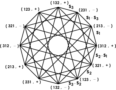
Figure 2. The labeled graph $\mathcal{G}_{2}$

Note that in Figure 2, the parallel edges have the same label.

Remark 3.3.

Let $V^{-}$ (resp. $V^{+}$) be a subset of $V(\mathcal{G}_{2})$ defined to be $\{(v,\varepsilon)\mid v\in S_{3},\varepsilon=-\text{(resp. $+$)}\}$, and $\mathcal{G}_{-}$ (resp. $\mathcal{G}_{+}$) be the labeled full subgraph of $\mathcal{G}_{2}$ with $V^{-}$ (resp. $V^{+}$) as a vertex set. Clearly $\mathcal{G}_{-}$ and $\mathcal{G}_{+}$ are isomorphic as a labeled graph to the labeled graph $\mathcal{A}_{3}$ associated with the root system of type $A_{2}$. Guillemin, Sabatini and Zara introduced the notion of a GKM fiber bundle in [5] (in a GKM fiber bundle, the total space, fiber and base space are all labeled graphs). In fact, it can be seen that $\mathcal{G}_{2}$ is the total space of a GKM fiber bundle, with fibers isomorphic to $\mathcal{A}_{2}$. In this sense it is natural to expect that the result of type $A_{2}$ plays a role when we determine the ring structure of $H_{T}^{*}(\mathcal{G}_{2})$ below.

4. Graph cohomology ring of $\mathcal{G}_{2}$

In this section, we state our main result which describes the ring structure of the graph cohomology ring of the labeled graph $\mathcal{G}_{2}$. We review the definition of the graph cohomology ring of a labeled graph first.

Definition 4.1.

Let $\mathcal{G}$ be a labeled graph with a label $\ell$ taking values in $H^{2}(BT)$ and let $W$ be the vertex set of $\mathcal{G}$. We identify $\bigoplus_{w\in W}H^{*}(BT)$ with $\operatorname{Map}(W,H^{*}(BT))$ where $Map(W,H^{*}(BT))$ is the set of all maps from $W$ to $H^{*}(BT)$. Then the graph cohomology $H^{*}(\mathcal{G})$ of $\mathcal{G}$ is defined to be the set of all $h\in\operatorname{Map}(W,H^{*}(BT))$ which satisfies the so-called “GKM condition”, namely for any two vertices $w$ and $w^{\prime}$ connected by an edge $e$, $h(w)-h(w^{\prime})$ is divisible by $\ell(e)$. The ring structure on $H^{*}(BT)$ induces a ring structure on $H^{*}_{T}(\mathcal{G})$.

To become familiar with a graph cohomology ring, we shall remember the graph cohomology ring of $\mathcal{A}_{3}$.

Example 4.2.

We define elements of $H_{T}^{*}(\mathcal{A}_{3})$ denoted by $\tau_{i}$’s and $t_{i}$’s as follows;

$$\tau_{i}(v):=t_{v(i)}\ \ \ \ \ t_{i}(v):=t_{i}\ \ \ \ \ \text{for any }v\in S_{3},\ \ i=1,2,3.$$

We regard an element in $\operatorname{Map}(W(\mathcal{A}_{3}),\mathbb{Z}[t_{1},t_{2},t_{3}])$ as a set of six polynomials in $t_{1},t_{2},t_{3}$ such that each polynomial corresponds to some vertex, because $W(\mathcal{A}_{3})=S_{3}$ has six verticies. So the elements $\tau_{i}$’s are described as the following figures.

One can easily check that $\tau_{i}$’s are in $H^{*}_{T}(\mathcal{A}_{3})$. One can also check that the elements $t_{i}$’s and $\tau_{i}$’s generate $H^{*}_{T}(\mathcal{A}_{3})$ as a ring, and

$$H_{T}^{*}(\mathcal{A}_{3})\cong\mathbb{Z}[\tau_{1},\tau_{2},\tau_{3},t_{1},t_{2},t_{3}]/J$$

where $J=<e_{i}(\tau)-e_{i}(t)\mid i=1,2,3>$ and $e_{i}(\tau)$ (resp. $e_{i}(t)$) is the $i^{th}$-elementary symmetric polynomial in $\tau_{1},\tau_{2},\tau_{3}$ (resp. $t_{1},t_{2},t_{3}$). (See [2].)

Now we consider elements in $H^{*}_{T}(\mathcal{G}_{2})$. We set $s_{w(i)}:=\varepsilon s_{v(i)}$ for $w=(v,\varepsilon)\in V(\mathcal{G}_{2})$. For each $i=1,2,3$, we define elements $\tau_{i}$, $t_{i}$ of $\operatorname{Map}(V(\mathcal{G}_{2}),\mathbb{Z}[t_{1},t_{2},t_{3}])$ by

(4.1) $$\tau_{i}(w):=s_{w(i)}=\varepsilon s_{v(i)},\ \ \ t_{i}(w):=t_{i}\ \ \ \text{for}\ \ \ w=(v,\varepsilon)\in V(\mathcal{G}_{2}).$$

One can check that $\tau_{i}$’s, $t_{i}$’s are elements of $H^{*}_{T}(\mathcal{G}_{2})$. We set $s_{i}:=t_{i}-t_{i+1}$ in $\operatorname{Map}(V(\mathcal{G}_{2}),\mathbb{Z}[t_{1},t_{2},t_{3}])$, namely $s_{i}(w)=(t_{i}-t_{i+1})(w)=t_{i}-t_{i+1}=s_{i}$, where $t_{4}=t_{1}$. In addition, we define an element $f$ of $\operatorname{Map}(V(\mathcal{G}_{2}),\mathbb{Z}[t_{1},t_{2},t_{3}])$ by

(4.2) $$f(w):=\left\{\begin{array}[]{ll}s_{1}s_{2}s_{3}&\text{for}\ \ \ w=(v,+)\\ 0&\text{for}\ \ \ w=(v,-).\\ \end{array}\right.$$

Clearly, $f$ is also an element of $H^{*}_{T}(\mathcal{G}_{2})$. Elements $\tau_{1}$ and $f$ are described in Figures 4 and 4.

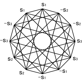
Figure 3. $\tau_{1}$

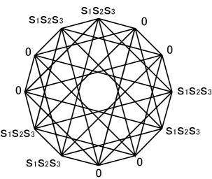
Figure 4. $f$

Remark 4.3.

The restriction of $\tau_{i}$ to the subgraph $\mathcal{G}_{+}$ (resp. $\mathcal{G}_{-}$) is $\tau_{i}$ (resp. $-\tau_{i}$) in $H_{T}^{*}(\mathcal{A}_{3})$. In other words $\tau_{i}$ in $H^{*}_{T}(\mathcal{G}_{2})$ is a lift of the $\tau_{i}$ in $H^{*}_{T}(\mathcal{A}_{3})$. The element $f$ comes from some element in the graph cohomology ring of the labeled graph of the base space. In fact, the labeled graph of the base space, denoted by $\mathcal{B}$, is described as Figure 6, and Figure 6 describes an element in $H^{*}_{T}(\mathcal{B})\subset\operatorname{Map}(V(\mathcal{B}),\mathbb{Z}[t_{1},t_{2},t_{3}])$. The element $f$ in $H^{*}_{T}(\mathcal{G}_{2})$ is the pullback of the element in Figure 6 by the projection $\mathcal{G}_{2}\to\mathcal{B}$.

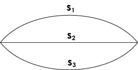
Figure 5.

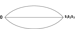
Figure 6.

Guillemin, Sabatini and Zara [5] construct module generators of the graph cohomology of the total space over the graph cohomology of the base space, by using module generators of the graph cohomology of fiber. (They consider the graph cohomology with $\mathbb{R}$ coefficient.)

Theorem 4.4.

Let $\mathcal{G}_{2}$ be the labeled graph associated with the root system $\Phi(G_{2})$ of type $G_{2}$. Then

$$H^{*}_{T}(\mathcal{G}_{2})=\mathbb{Z}[\tau_{1},\tau_{2},\tau_{3},t_{1},t_{2},t_{3},f]/I,$$

where $I=<e_{1}(\tau),e_{2}(\tau)-e_{2}(s),2f-e_{3}(\tau)-e_{3}(s),f^{2}-fe_{3}(s)>$, and $e_{i}(\tau)$ $($resp. $e_{i}(s)$ $)$ is the $i^{th}$ elementary symmetric polynomial in $\tau_{1},\tau_{2},\tau_{3}$ $($resp. $s_{1},s_{2},s_{3}$ $)$.

The rest of the paper is devoted to the proof of Theorem 4.4.

Lemma 4.5.

$H^{*}_{T}(\mathcal{G}_{2})$ is generated by $\tau_{1},\tau_{2},\tau_{3}$, $t_{1},t_{2},t_{3}$ and $f$ as a ring.

Proof.

The idea of the proof of the lemma is same as that of Lemma 3.2 in [2].

Claim 4.6.

For any homogeneous element $h$ of $H^{*}_{T}(\mathcal{G}_{2})$, there is a polynomial $G$ in $\tau_{i}$’s and $t_{i}$’s such that the restrictions of $h$ and $G$ to the subgraph $\mathcal{G}_{-}$ coincide.

Proof of Claim. We set

$$V_{i}^{-}:=\{(v,\varepsilon)\in S_{3}\times\{\pm\}\mid v(i)=3,\varepsilon=-\}\quad\text{for}\quad i\in[3].$$

Let $2k$ be the degree of $h\in H^{*}_{T}(\mathcal{G}_{2})$ and

$$1\leq q\leq\min\{k+1,3\}$$

and assume that

$$h(w_{i})=0\ \ \ \text{for any }w_{i}\in V_{i}^{-}\ \text{whenever}\ \ i<q.$$

For any $w=(v,-)\in V_{q}^{-}$, there is a unique vertex $w_{i}=(v_{i},-)\in V_{i}^{-}$ for each $1\leq i<q$ such that $w$ and $w_{i}$ are connected by an edge labeled by $s_{w(i)}-s_{w(q)}=s_{w(i)}+s_{3}$. (Namely $v=v_{i}(i,q)$.) Then $h(w)-h(w_{i})=h(w)$ is divisible by $s_{w(i)}+s_{3}$ for $i<q$, so there is a homogeneous polynomial $g_{w}\in\mathbb{Z}[t_{1},t_{2},t_{3}]$ of degree $2(k-q+1)$ such that

(4.3) $$h(w)=g_{w}\prod_{i=1}^{q-1}(s_{w(i)}+s_{3}).$$

On the other hand, since $(\tau_{k}+s_{3})(u)=s_{u(k)}+s_{3}$ for any $u\in V(\mathcal{G}_{2})$,

(4.4) $$\prod_{i=1}^{q-1}(\tau_{i}+s_{3})(u)=\prod_{i=1}^{q-1}(s_{u(i)}+s_{3}).$$

In particular, when $u$ is in $V_{i}^{-}$ for $i<q$, (4.4) is equal to $0$ since $s_{u(i)}=-s_{3}$. So, it follows from (4.3) and (4.4) that

(4.5) $$\left(h-g_{w}\prod_{i=1}^{q-1}(\tau_{i}+s_{3})\right)(u)=0,$$

whenever $u\in V_{i}^{-}$ for $i<q$ or $u=w$. We set

(4.6) $$h^{\prime}:=h-g_{w}\prod_{i=1}^{q-1}(\tau_{i}+s_{3}).$$

Note that

(4.7) $$h^{\prime}(u)=0\quad\text{if $u\in V_{i}^{-}$ for $i<q$ or $u=w$.}$$

Let $w^{\prime}$ be the other vertex in $V_{q}^{-}$. (Namely, $V_{q}^{-}=\{w,w^{\prime}\}$.) Then $w$ and $w^{\prime}$ are connected by an edge labeled by $s_{1}-s_{2}$ and there is a unique vertex $w_{i}^{\prime}=(v_{i}^{\prime},-)\in V_{i}^{-}$ for each $1\leq i<q$ such that $w^{\prime}$ and $w_{i}^{\prime}$ are connected by an edge labeled by $s_{w^{\prime}(i)}-s_{w^{\prime}(q)}=s_{w^{\prime}(i)}+s_{3}$, so $h^{\prime}(w^{\prime})-h^{\prime}(w)=h^{\prime}(w^{\prime})$ is divisible by $s_{1}-s_{2}$ and $s_{w^{\prime}(i)}+s_{3}$. Therefore, there is a homogeneous polynomial $g_{w^{\prime}}\in\mathbb{Z}[t_{1},t_{2},t_{3}]$ of degree $2(k-q)$ such that

(4.8) $$h^{\prime}(w^{\prime})=(s_{1}-s_{2})g_{w^{\prime}}\prod_{i=1}^{q-1}(s_{w^{\prime}(i)}+s_{3}).$$

On the other hand, for $j\in[3]\setminus\{q\}$,

(4.9) $$\left(\tau_{j}-s_{w(j)}\right)(w^{\prime}) = s_{w^{\prime}(j)}-s_{w(j)}=\delta(s_{1}-s_{2})$$

(4.10) $$\left(\tau_{j}-s_{w(j)}\right)(w) = s_{w(j)}-s_{w(j)}=0,$$

where $\delta=\pm 1$ and $\delta$ depends on $w$. Thus, it follows from (4.4), (4.8), (4.9) and (4.10) that

$$\left(h^{\prime}-(\tau_{j}-s_{w(j)})(\delta g_{w^{\prime}})\prod_{k=1}^{q-1}(\tau_{k}+s_{3})\right)(u)=0.$$

for $u\in V_{i}^{-}$ whenever $i\leq q$. Therefore, putting $H=g_{w}+(\tau_{j}-s_{w(j)})(\delta g_{w^{\prime}})$, and subtracting the polynomial $H\Pi_{k=1}^{q-1}(\tau_{j}+s_{3})$ from $h$, we may assume that

$$h(u)=0\ \ \ \text{for any }\ \ u\in V_{i}^{-}\ \ \ \text{whenever}\ \ \ i<q+1.$$

The above argument implies that $h$ finally takes zero on all vertices in $V^{-}$ by subtracting a polynomial in $\tau_{i}$’s and $t_{i}$’s, and this completes the proof of the claim.

The claim allows us to assume that our homogeneous element $h$ in $H^{*}_{T}(\mathcal{G}_{2})$ satisfies $h(u)=0$ for all $u\in V^{-}$. Any $w=(v,+)\in V^{+}$ has a unique edge which connects $w$ and some $w_{i}=(v_{i},-)\in V_{i}^{-}$ for each $i\in[3]$, and the edge has a label $s_{w(k)}$ where $k$ is determined by $v(k)=v_{i}(k)$. Namely, $h(w)-h(w_{i})=h(w)$ is divisible by $s_{w(k)}$, thus, there is a homogeneous polynomial $p_{w}$ of $\mathbb{Z}[t_{1},t_{2},t_{3}]$ such that

$$h(w)=s_{1}s_{2}s_{3}p_{w}.$$

In addition the collection of polynomials $\{p_{w}\}$ satisfies the GKM condition in $\mathcal{G}_{+}$. In fact, for any vertices $w$ and $w^{\prime}$ in $V^{+}$ connected by an edge with label $s_{i}-s_{j}$ for some $i,j\in[3]$, it follows from the definition of $H^{*}_{T}(\mathcal{G}_{2})$ that $h(w)-h(w^{\prime})=s_{1}s_{2}s_{3}(p_{w}-p_{w^{\prime}})$ is divisible by $s_{i}-s_{j}$. So $p_{w}-p_{w^{\prime}}$ is divisible by the label $s_{i}-s_{j}$. Then the same argument as in the proof of the claim above shows that there is a polynomial $H^{\prime}$ in $\tau_{i}$’s and $t_{i}$’s such that $H^{\prime}(w)=p_{w}$ for $w\in V^{+}$. Therefore,

$$(h-H^{\prime}f)(w)=0\ \ \ \text{for any}\ \ \ w\in V(\mathcal{G}_{2}).$$

This completes the proof of the lemma. ∎

Remember that the Hilbert series of a graded ring $A^{*}=\oplus_{j=0}^{\infty}A^{j}$, where $A^{j}$ is the degree $j$ part of $A^{*}$ and of finite rank over $\ \mathbb{Z}$, is a formal power series defined by

$$F(A^{*},x):=\sum_{j=0}^{\infty}(\operatorname{rank}_{\mathbb{Z}}A^{j})x^{j}.$$

Lemma 4.7.

$$F(H^{*}_{T}(\mathcal{G}_{2}),x)=\frac{1}{(1-x^{2})^{3}}(1+x^{2})(1+x^{2}+x^{4})(1+x^{6})$$

Proof.

We set $d(k):=\operatorname{rank}H^{2k}_{T}(\mathcal{G}_{2})$ and $r(k):=\operatorname{rank}\mathbb{Z}[t_{1},t_{2},t_{3}]^{2k}$, where $\mathbb{Z}[t_{1},t_{2},t_{3}]^{2k}$ is the set of homogeneous polynomials of degree $2k$. We note that the degree of $t_{i}$ is $2$. For $h\in H^{2k}_{T}(\mathcal{G}_{2})$, assume that there is some $q\in[3]$ such that

$$h(w)=0\ \ \text{for}\ \ w\in V^{-}_{i}\ \ \text{whenever}\ \ i<q.$$

Then, the proof of the claim in Lemma 4.5 shows that there is a polynomial $H$ in $\tau_{i}$’s and $t_{i}$’s such that

$$(h-H)(w)=0\quad\text{for}\quad w\in V^{-}_{i}\quad\text{whenever}\ \ i\leq q,$$

and that the polynomial $H$ is of the form

$$H=\left(g_{w}+\delta(\tau_{j}-s_{w(j)})g_{w^{\prime}}\right)\prod^{q-1}_{k=1}(\tau_{k}+s_{3})$$

where $g_{w}$ and $g_{w^{\prime}}$ are some polynomials in $t_{1},t_{2},t_{3}$, and the degree of $g_{w}$ (resp. $g_{w^{\prime}}$) is $2(k-q+1)$ (resp. $2(k-q)$). Therefore the rank of the additive group consisting of all such polynomials $H$ is given by

$$r(k-q+1)+r(k-q).$$

Similarly, assume that there is some $q\in[3]$ such that

$$h(w)=0\ \ \text{for}\ \ w\in V^{-}\ \ \text{or}\ \ w\in V^{+}_{i}\ \ \text{whenever}\ \ i<q,$$

where $V^{+}_{i}=\{(v,+)\ \mid\ v(i)=3\}.$ Then, the proof of Lemma 4.5 shows that there is a polynomial $H^{\prime}$ in $\tau_{i}$’s, $t_{i}$’s and $f$ such that

$$(h-H^{\prime})(w)=0\quad\text{for}\quad w\in V^{-}\quad\text{or}\quad w\in V^{+}_{i}\quad\text{whenever}\quad i\leq q,$$

and that the polynomial $H^{\prime}$ is of the form

$$H^{\prime}=s_{1}s_{2}s_{3}\left(g^{\prime}_{w}+\delta(\tau_{j}-s_{w(j)})g^{\prime}_{w^{\prime}}\right)\prod^{q-1}_{k=1}(\tau_{k}+s_{3})$$

where $w$ and $w^{\prime}$ are the two vertices of $V^{+}_{q}$ and $g^{\prime}_{w}$ and $g^{\prime}_{w^{\prime}}$ are some polynomials in $t_{1},t_{2},t_{3}$, and the degree of $g^{\prime}_{w}$ (resp. $g^{\prime}_{w^{\prime}}$) is $2(k-2-q)$ (resp. $2(k-3-q)$). Thus, the rank of the the additive group consisting of all such polynomials $H^{\prime}$ is given by

$$r(k-2-q)+r(k-3-q).$$

Let $G^{+}_{q}$ (resp. $G^{-}_{q}$) be the the additive group consisting of all polinomials $h$ of degree $2k$ such that

$$h(w)=0\ \ \text{for}\ \ w\in V^{-}\ \ \text{or}\ \ w\in V^{+}_{i}\ \ \text{whenever}\ \ i<q$$

$$\text{(resp. }h(w)=0\ \ \text{for}\ \ w\in V^{-}_{i}\text{whenever}\ \ i<q\text{\ )}.$$

Then, the rank of $G^{+}_{3}$ is $r(k-5)+r(k-6)$ by the above argument. The rank of $G^{+}_{2}$ is equal to $\operatorname{rank}G^{+}_{3}$ plus the rank of additive group consisting of all polynomial $H^{\prime}$ such that

$$(h-H^{\prime})(w)=0\quad\text{for}\quad w\in V^{-}\quad\text{or}\quad w\in V^{+}_{i}\quad\text{whenever}\quad i\leq 2,$$

so the rank of $G^{+}_{2}$ is $\operatorname{rank}G^{+}_{3}+r(k-4)+r(k-5)$. Similarly, the rank of $G^{+}_{1}$ is equal to $\operatorname{rank}G^{+}_{2}$ plus $r(k-3)+r(k-4)$, namely

(4.11) $$\operatorname{rank}G^{+}_{1}=\sum_{i=4}^{6}(r(i)+r(i-1)).$$

In the same way, we have

(4.12) $$\operatorname{rank}G^{-}_{3}=\operatorname{rank}G^{+}_{1}+r(k-2)+r(k-3),$$

and

(4.13) $$\operatorname{rank}G^{-}_{q}=\operatorname{rank}G^{-}_{q+1}+r(k-q+1)+r(k-q)\quad\text{for }q=1,2.$$

Therefore, it follows from (4.11), (4.12) and (4.11) that

$$d(k)=\operatorname{rank}G^{-}_{1}=\sum_{i=k}^{k-5}\Big{(}r(i)+r(i-1)\Big{)}=r(k)+2\sum_{i=k-5}^{k-1}r(i)+r(k-6)$$

where $r(i)=0$ for $i<0$. Namely,

$$d(k)=\left\{\begin{array}[]{ll}r(0)&\text{for}\ \ \ k=0\\ 2\sum_{i=0}^{k-1}r(i)+r(k)&\text{for}\ \ \ 1\leq k\leq 5\\ r(k-6)+2\sum_{i=k-5}^{k-1}r(i)+r(k)&\text{for}\ \ \ k>5.\\ \end{array}\right.$$

Therefore,

$$F(H^{*}_{T}(\mathcal{G}_{2}),x) = \sum_{k=0}^{\infty}d(k)x^{2k}$$

$$= r(0)+\sum_{k=1}^{5}\left(2\sum_{i=0}^{k-1}r(i)+r(k)\right)x^{2k}$$

$$\quad+\sum_{k=6}^{\infty}\left(r(k-6)+2\sum_{i=k-5}^{k-1}r(i)+r(k)\right)x^{2k}$$

$$= \sum_{k=0}^{\infty}r(k)x^{2k}+\sum_{k=6}^{\infty}r(k-6)x^{2k}$$

$$\quad+2\left(\sum_{k=1}^{5}\sum_{i=0}^{k-1}r(i)x^{2k}+\sum_{k=6}^{\infty}\sum_{i=k-5}^{k-1}r(i)x^{2k}\right)$$

$$= (1+x^{12})(r(0)+r(1)x^{2}+r(2)x^{4}+\cdots)$$

$$\ +2(x^{2}+x^{4}+x^{6}+x^{8}+x^{10})(r(0)+r(1)x^{2}+r(2)x^{4}+\cdots)$$

$$= (1+2x^{2}+2x^{4}+2x^{6}+2x^{8}+2x^{10}+x^{12})F(\mathbb{Z}[t_{1},t_{2},t_{3}],x)$$

$$= (1+x^{2})(1+x^{2}+x^{4})(1+x^{6})F(\mathbb{Z}[t_{1},t_{2},t_{3}],x)$$

$$= \frac{1}{(1-x^{2})^{3}}(1+x^{2})(1+x^{2}+x^{4})(1+x^{6}),$$

proving the lemma. ∎

We abbreviate the polynomial ring $\mathbb{Z}[\tau_{1},\tau_{2},\tau_{3},t_{1},t_{2},t_{3},f]$ as $\mathbb{Z}[\tau,t,f]$. The canonical map $\mathbb{Z}[\tau,t,f]\to H^{*}_{T}(\mathcal{G}_{2})$ is a grade preserving homomorphism which is surjective by Lemma 4.5. It easily follows from (4.1) and (4.2) that

(4.14) $$e_{1}(\tau) = 0,$$

(4.15) $$e_{2}(\tau)-e_{2}(s) = 0,$$

(4.16) $$2f-e_{3}(\tau)-e_{3}(s) = 0,\quad\quad\text{and}$$

(4.17) $$f^{2}-fe_{3}(s) = 0.$$

Therefore the canonical map above induces a grade preserving epimorphism

(4.18) $$\mathbb{Z}[\tau,t,f]/I\to H_{T}^{*}(\mathcal{G}_{2}),$$

where

$$I=<e_{1}(\tau),e_{2}(\tau)-e_{2}(s),2f-e_{3}(\tau)-e_{3}(s),f^{2}-fe_{3}(s)>.$$

We note that $\mathbb{Z}[\tau,t,f]/I$ is a $\mathbb{Z}[t]$-module in a natural way.

Lemma 4.8.

$\mathbb{Z}[\tau,t,f]/I$ is generated by $\prod_{k=1}^{3}\tau_{k}^{i_{k}}f^{j}$ for $0\leq i_{k}\leq 3-k$ and $j=0,1$ as a $\mathbb{Z}[t]-$module.

Proof.

Clearly the elements $\Pi_{k=1}^{3}\tau_{k}^{i_{k}}f^{j}$ with no restriction on exponents, generate $\mathbb{Z}[\tau,t,f]/I$ as a $\mathbb{Z}[t]-$module. The identity (4.14) means

(4.19) $$\tau_{3}=-\tau_{1}-\tau_{2}.$$

By using (4.19), we have

$$e_{2}(\tau)=\tau_{1}\tau_{2}+\tau_{3}(\tau_{1}+\tau_{2})=\tau_{1}\tau_{2}-(\tau_{1}+\tau_{2})^{2}=-\tau_{1}^{2}-\tau_{2}^{2}-\tau_{1}\tau_{2}.$$

Therefore, $\tau_{2}^{2}=-\tau_{1}^{2}-\tau_{1}\tau_{2}-e_{2}(\tau),$ and hence

(4.20) $$\tau_{2}^{2}=-\tau_{1}^{2}-\tau_{1}\tau_{2}-e_{2}(s)$$

by (4.15). It follows from (4.19) and (4.20) that

$$e_{3}(\tau) = \tau_{1}\tau_{2}\tau_{3}$$

$$= -\tau_{1}\tau_{2}(\tau_{1}+\tau_{2})$$

$$= -\tau_{1}^{2}\tau_{2}-\tau_{1}\tau_{2}^{2}$$

$$= -\tau_{1}^{2}\tau_{2}+\tau_{1}(\tau_{1}^{2}+\tau_{1}\tau_{2}+e_{2}(s))$$

$$= \tau_{1}^{3}+\tau_{1}e_{2}(s),$$

Therefore $\tau_{1}^{3}=-\tau_{1}e_{2}(s)+e_{3}(\tau)$ and hence

(4.21) $$\tau_{1}^{3}=-\tau_{1}e_{2}(s)+2f-e_{3}(s)$$

by (4.16). Therefore, $\tau_{k}^{3-k+1}$ is written as (4.19), (4.20) and (4.21), satisfying that the exponent of $\tau_{k}$ is less than or equal to $3-k$ and that of $f$ is 0 or 1. In addition, $f^{2}$ is written as (4.17), so we can always assume the exponent of $f$ to be 0 or 1. This completes the proof of the lemma. ∎

Now we are in a position to complete the proof of Theorem 4.4.

Proof of Theorem 4.4.

If two formal power series $a(x)=\sum_{i=0}^{\infty}a_{i}x^{i}$ and $b(x)=\sum_{i=0}^{\infty}b_{i}x^{i}$ in $x$ with real coefficients $a_{i}$ and $b_{i}$ satisfy $a_{i}\leq b_{i}$ for every $i$, then we express this as $a(x)\leq b(x)$.

The Hilbert series of the free $\mathbb{Z}[t]$-module generated by $\prod_{k=1}^{3}\tau_{k}^{i_{k}}f^{j}$ is given by $\frac{1}{(1-x^{2})^{3}}x^{2(\sum_{k=1}^{3}i_{k}+3j)}$, so it follows from Lemma 4.8 that

(4.22) $$F(\mathbb{Z}[\tau,t,f]/I,x)\leq\frac{1}{(1-x^{2})^{3}}\sum_{0\leq i_{1}\leq 2,\ 0\leq i_{2}\leq 1}x^{2(i_{1}+i_{2})}\sum_{j=0}^{1}x^{6j}$$

and the equality holds above if and only if $\mathbb{Z}[\tau,t,f]/I$ is free as a $\mathbb{Z}[t]$-module. Here the right hand side in (4.22) above is equal to

$$\frac{1}{(1-x^{2})^{3}}(1+x^{2})(1+x^{2}+x^{4})(1+x^{6})$$

which agrees with $F(H^{*}_{T}(\mathcal{G}_{2}),x)$ by Lemma 4.7. Therefore $F(\mathbb{Z}[\tau,t,f]/I,x)\leq F(H^{*}_{T}(\mathcal{G}_{2}),x)$. On the other hand, the surjectivity of the map (4.18) implies the opposite inequality. Therefore $F(\mathbb{Z}[\tau,t,f]/I,x)=F(H^{*}_{T}(\mathcal{G}_{2}),x)$. This means that the inequality in (4.22) must be an equality and hence $\mathbb{Z}[\tau,t,f]/I$ is free as a $\mathbb{Z}[t]$-module, in particular, as a $\mathbb{Z}$-module. Since the map in (4.18) is surjective and $F(\mathbb{Z}[\tau,t,f]/I,x)=F(H^{*}_{T}(\mathcal{G}_{2}),x)$, we conclude that the map in (4.18) is actually an isomorphism. This proves Theorem 4.4. ∎

Acknowledgment. The author takes this opportunity to thank her Ph.D. supervisor Mikiya Masuda for sparing his precious time and give constructive comments throughout the process of writing this paper. I also thank Shizuo Kaji and Hiroshi Naruse, who gave me the opportunity to consider this problem on the flag manifold of type $G_{2}$. Finally, Megumi Harada gave me lots of valuable advice both about mathematics and writing in English.

References

- [1] D. E. Anderson, Chern class formulas for Schubert loci, Trans. Amer. Math. Soc. 363 (2011) 6615-6646.
- [2] Y. Fukukawa, H. Ishida and M. Masuda, The cohomology ring of the GKM graph of a flag manifold of classical type, arXiv:1102.4476
- [3] M. Goresky, R. Kottwitz and R. MacPherson, Equivariant cohomology, Koszul duality and the localisation theorem, Invent. Math. 131 (1998) 25–83.
- [4] V. Guillemin, T. Holm and C. Zara, A GKM description of the equivariant cohomology ring of a homogeneous space, J. Algebraic Combin. 23 (2006), 21–41.
- [5] V. Guillemin, S. Sabatini and C. Zara, Cohomology of GKM fiber bundles, J. Algebraic Combin. (2011), 1–41.
- [6] V. Guillemin and C. Zara, 1-skeleta, Betti numbers and equivariant cohomology, Duke Math. J. 107 (2001) 283–349.
- [7] M. Harada, A. Henriques and T. Holm, Computation of generalized equivariant cohomologies of Kac-Moody flag varieties, Adv. Math. 197 (2005), 198–221.