Minimizing gauge-functional for 2-d gravity and string theory
Laurent Baulieu
Theoretical Division CERN
LPTHE Université Pierre et Marie Curie
Daniel Zwanziger

Physics Department, New York University

We show the existence of a minimizing procedure for selecting a unique representative on the orbit of any given Riemann surface that contributes to the string partition function. As it must, the procedure reduces the string path integral to a final integration over a particular fundamental domain, selected by the choice of the minimizing functional. This construction somehow demystifies the Gribov question.

1 Introduction

In this article, we describe a procedure for gauge-fixing the 2d-gravity gauge invariance [1] with a geometrical meaning that is as transparent as possible. The aim is to find a definition that escapes the Gribov question [2] and, more precisely, to select unambiguosuly a single representative on the orbits of the conformal classes of metrics of Riemann surfaces.

A better understanding of the gauge-fixing is useful for the predictions of string theory. For instance, for on-shell string observables, the singularities at the boundaries of the moduli space of string worldsheets are the source of infra-red divergencies of the 4-dimensional quantum field theory limit. An unambiguous string gauge-fixing method is certainly needed.

We will show the existence of a minimizing procedure for selecting a unique representative on the orbit of any given Riemann surface that contributes to the partition function, while making sure that a BRST symmetry is maintained. The procedure selects among all representatives of the worldsheet in the Teichmüller space a particular fundamental domain, which is made of representatives that are at absolute minimum distance of a reference worldsheet. We will use the framework of the Beltrami parametrization of string 2d-worldsheets (and its extension for the superstring).

The method holds for any given fixed genus. For the torus, the procedure may be tuned to select the first fundamental domain of the Poincaré disk. In this method, the obvious inconsistencies of the Faddeev–Popov method in the “conformal gauge”, and possible Gribov copies are successfully eliminated.

The Beltrami parametrization of the 2-dimensional metrics in string theory was introduced in 1986 for a clearer definition of the path integral of the 2d-gravity field [3][4]. It gives a better understanding of the factorization of left and right movers and of the the conformal anomaly of string theory. Its use respects the context of local quantum field theory, and allows the control of the conformal Ward identities. The Beltrami parametrization gives a formally very strong parallel between Yang–Mills and string theory BRST technologies.

One motivation of this work is that string theory is a simpler arena than Yang–Mills theory for finding unambiguous gauge–fixings, beyond the limitation of the Faddeev–Popov method. Earlier ideas suggested that, for defining the Yang–Mills path integral over $\cal A$/$\cal G$, in the theory, one should pick out the absolute minimum of the norm $\int d^{4}x\hbox{Tr}~{}A_{\mu}A^{\mu}$ on each orbit of the space of gauge field configuration $\{A_{\mu}\}$. In string theory, one can do a careful and precise analysis. The result suggests that one should perhaps use a more refined minimizing function $\int d^{4}xf(\hbox{Tr}~{}A_{\mu}A^{\mu})$, where the function $f$ is introduced to avoid spurious divergencies that do not concentrate at the boundary of the moduli space of gauge field configurations. In fact, for a given Riemann surface, we will show that one can choose the following minimizing function

$$F[\mu^{z}_{\bar{z}},\mu^{\bar{z}}_{z}]=\int_{\Sigma}\rho_{z{\bar{z}}}(z,{\bar{z}})dzd{\bar{z}}\ \frac{1}{{1-|\mu|^{2}}}\ln\frac{1-|\mu|}{1+|\mu|}.$$ (1)

where $\mu^{z}_{\bar{z}}$ is the Beltrami differential and the factor $\rho_{z{\bar{z}}}(z,{\bar{z}})$ is a universal measure that depends only on the genus of the Riemann surface.

The paper is organized as follows. We first recall basic formulas for the Beltrami parametrization in string theory. We then explain the gauge-fixing procedure as a minimizing principle of a relevant functional on the orbit of each Riemann surface. We show how it leads to a BRST-invariant action. The functional expresses the distance between an arbitrarily chosen point in the Teichmüller space of a reference surface (at a fixed genus) and any given possible representative of the 2d-metrics of a surface, defined modulo local dilatations. The gauge fixing consists in choosing the metric that minimizes this distance. The method can be explored in great detail for the torus. Interestingly, a careful choice of the distance must be done to avoid spurious Gribov-type problems. For higher genus, the method is geometrically well-defined, but one faces in practice the complication and/or our ignorance about the nature and the details of modular groups and fundamantal domains. Technical complications are obviously foreseen for $g>1$, even at $g=2$. A formal generalisation of the Nauenberg–Lee–Bloch–Nordsieck arguments to string theory should be possible in which a cancellation of divergent contributions occurs between amplitudes of different genus, with insertions of “soft” vertex operators.

Other formulations of string theory exist where one can find the untwining of the geometry of Riemann surfaces and the quantum field theory of strings, such as the light-cone or the Witten formulation of open string field theory, see for instance [6]. However, the conformal gauge approach, as it is formulated in this paper from a minimizing principle, has the great advantage of combining in a rather satisfactorying way a precise description of Riemann surface orbits and the basic properties of 2-dimensional local quantum field theory.

2 Beltrami parametrization for strings

2.1 Definition and the choice of a coordinate system

Once one understands, following Polyakov [1], that the propagation of a string on a given manifold sweeps out quantum mechanically all possible worldsheets that can be embedded in a given target space, with possible emissions of other strings, one needs a parametrization of 2-dimensional manifolds that is as handy as possible, in order to perform a path integral over all the metric fluctuations. Such a parametrization is provided by the Beltrami differential, which completely avoids the use of the scalar part of the metric, and provides an appropriate local field variable for the path integral.

The geometrical data are as follows. One considers a metric on an arbitrary smooth compact 2-dimensional Riemann surface $\Sigma(z,{\bar{z}})$ without boundary, and of genus $g$. Here $(z,{\bar{z}})$ denotes at each point a fixed local set of complex analytic coordinates on $\Sigma$. The Beltrami differential $\mu^{z}_{\bar{z}}$ and its complex conjugate $\mu^{\bar{z}}_{z}$ are defined by the following parameterization of the 2d-metric on $\Sigma$,

$$ds^{2}=\Big{(}\exp 2\Phi\Big{)}(dz+\mu^{z}_{\bar{z}}d{\bar{z}})(d{\bar{z}}+\mu^{\bar{z}}_{z}dz),$$ (2)

where $\exp 2\Phi(z,{\bar{z}})$ is the conformal factor of the metric in this choice of coordinates. The transformation law of $\mu^{z}_{\bar{z}}$ and $\mu^{\bar{z}}_{z}$ under dilatations is zero. The infinitesimal transformations of $\mu^{z}_{\bar{z}}$ and $\mu^{\bar{z}}_{z}$ will be given shortly in the form of a BSRT symmetry.

A minimal set of patches for a surface of a given genus can be generally obtained. The Beltrami differentials are a set of local functions in each patch, that are globally identified on their common boundaries. When one changes the system of coordinates, $z,{\bar{z}}\to z^{\prime},{{\bar{z}}}^{\prime}$, the shape of the patches changes, but the deformation of their boundaries is obtained by the repametrization in each path, and the identification on the boundaries of neighboring patches still holds.

New coordinates $Z$ and $\bar{Z}$ are defined by

$$dZ=\rho^{Z}_{z}(\mu^{z}_{\bar{z}},z,\bar{z})(dz+\mu^{z}_{\bar{z}}d{\bar{z}})\ \ \ \ \ \ \ d\bar{Z}=\bar{\rho}^{\bar{Z}}_{\bar{z}}(\mu^{\bar{z}}_{z},z,\bar{z})(d{\bar{z}}+\mu^{\bar{z}}_{z}dz).$$ (3)

where $\rho^{Z}_{z}$ is an integrating factor. Since $d^{2}=0$, $\rho^{Z}_{z}$ satisfies the differential equation $(\partial_{{\bar{z}}}-\mu^{z}_{\bar{z}}\partial_{z})\ln\rho^{Z}_{z}=\partial_{z}\mu^{z}_{\bar{z}}$ and functionally depends only on $\mu^{z}_{\bar{z}}$.

To define the reparametrization- and dilatation-invariant quantum field theory that corresponds to a given Lagrangian, the general approach is to choose once and for all a fixed set of coordinates. This means adopting the point of view of active gauge transformations on the fields, without explicitly changing coordinates. From now on, we will thus assume that all fields, including the Beltrami differentials, only transform under active symmetries, such as the BRST symmetry. All formulas must be written in such a way that they can be put automatically in correspondence with another system of coordinates. One must not confuse the BRST symmetry of the theory and the possibility of choosing different sets of coordinates for defining the path integral. The quantum field theory is defined as satisfying all Ward identities corresponding to the BRST symmetry, in the absence of contradictions due to a possible non-vanishing anomaly. Observables are defined from the cohomology of the BRST symmetry.

2.2 2d-action and Beltrami parametrization

For any given local lagrangian depending on the 2d-metric $g^{\alpha\beta}$ on $\Sigma$ and on fields whose arguments are coordinates on $\Sigma$, one can replace the dependence on $g^{\alpha\beta}$ by dependence on $\mu^{z}_{\bar{z}}$, $\mu^{\bar{z}}_{z}$ and $\Phi$. For instance, the globally well-defined two-form curvature of $\Sigma$ is

$$R_{z,{\bar{z}}}=\partial_{z}\partial_{\bar{z}}\Phi+\partial_{z}\partial_{z}\mu^{z}_{\bar{z}}+\partial_{\bar{z}}\partial_{\bar{z}}\mu^{\bar{z}}_{z}+{\cal O}(\mu^{2})$$ (4)

Conformally-invariant quantities can depend only on $\mu^{z}_{\bar{z}}$ and $\mu^{\bar{z}}_{z}$. Given the string field $X(z,{\bar{z}})$, a quick computation shows that the Polyakov action is given simply by

$$\int_{\Sigma}dX\wedge*dX=\int_{\Sigma}d^{2}z\sqrt{g}g^{\alpha\beta}\partial_{\alpha}X\partial_{\beta}X=\int d^{2}z\frac{(\partial_{\bar{z}}-\mu^{z}_{\bar{z}}\partial_{z})X(\partial_{z}-\mu^{\bar{z}}_{z}\partial_{\bar{z}})X}{1-\mu^{z}_{\bar{z}}\mu^{\bar{z}}_{z}}.$$ (5)

For this action, the path integral over the fields of 2d-gravity only involves the Beltrami differential components $\mu^{z}_{\bar{z}}$ and $\mu^{\bar{z}}_{z}$. The gauge-fixing of Weyl transformations is trivial, provided that there is no conformal anomaly because, for such conformally-invariant actions, the Faddeev-Popov determinant associated to setting $\Phi=0$ equals one. These properties made it possible in the mid-80’s to rederive, within the context of local quantum field theory, many conventional results of string theory that had been obtained previously by other methods, e.g., [3][4]. In fact, $\mu^{z}_{\bar{z}}$, after its gauge fixing, is nothing but the source of the energy tensor component $T_{zz}$, but to do this gauge-fixing, one must address global issues. Moreover $\Phi$ is an irrelevant field variable, not seen by conformal invariance.

2.3 Factorization property and Beltrami parametrization

The Beltrami parametrization is well adapted to the factorization property of left and right movers and to the conformal invariance on the worldsheet that lie at the heart of string theory. The (active) gauge transformations of $\mu^{z}_{\bar{z}}$ and $\mu^{\bar{z}}_{z}$ under an infinitesimal local 2d-diffeomorphism with vector field $({\epsilon^{z}},{\epsilon^{\bar{z}}})$ are

$$\delta\mu^{z}_{\bar{z}} = \partial_{\bar{z}}\epsilon^{z}+\epsilon^{z}\partial_{z}\mu^{z}_{\bar{z}}-\mu^{z}_{\bar{z}}\partial_{z}\epsilon^{z}$$

$$\delta\mu^{\bar{z}}_{z} = \partial_{z}\epsilon^{\bar{z}}+\epsilon^{\bar{z}}\partial_{\bar{z}}\mu^{\bar{z}}_{z}-\mu^{\bar{z}}_{z}\partial_{\bar{z}}\epsilon^{\bar{z}}.$$ (6)

We observe that the fields $\mu^{z}_{\bar{z}}(z,{\bar{z}})$ and $\mu^{\bar{z}}_{z}(z,{\bar{z}})$ are invariant under local dilatations, and also that the general infinitesimal variation of $\mu^{z}_{\bar{z}}$ depends only on the single local parameter $\epsilon^{z}$, and on $\mu^{z}_{\bar{z}}$. This is known as the factorization property. For the purpose of BRST-invariant quantization, one replaces $(\epsilon^{z},\epsilon^{\bar{z}})$ by the anticommuting Faddeev-Popov ghost field $(c^{z},c^{{\bar{z}}})$ and defines the active BRST symmetry that corresponds to the above infinitesimal transformations

$$s\mu^{z}_{\bar{z}} = \partial_{\bar{z}}c^{z}+c^{z}\partial_{z}\mu^{z}_{\bar{z}}-\mu^{z}_{\bar{z}}\partial_{z}c^{z}\ \ \ \ \ \ \ \ \ \ sc^{z}=c^{z}\partial_{z}c^{z}$$

$$s\mu^{\bar{z}}_{z} = \partial_{z}c^{{\bar{z}}}+c^{{\bar{z}}}\partial_{\bar{z}}\mu^{\bar{z}}_{z}-\mu^{\bar{z}}_{z}\partial_{\bar{z}}c^{{\bar{z}}}\ \ \ \ \ \ \ \ \ \ sc^{{\bar{z}}}=c^{{\bar{z}}}\partial_{\bar{z}}c^{{\bar{z}}}$$ (7)

The action of $s$ is nilpotent on all fields, $s^{2}=0$. According to the general BRST method for local gauge-fixing, the small diffeomorphism invariance of e.g. the Polyakov action can be locally gauged-fixed in the path integral by adding to the invariant classical action an $s$-exact term, which imposes a condition on $\mu^{z}_{\bar{z}}$ and $\mu^{\bar{z}}_{z}$ that allows one to do the path integral. This gauge-fixing term can be chosen to respect the left-right independence on the worldsheet. However, as in the case of the Yang–Mills theory, no local gauge function can be chosen that is globally well defined; zero modes can occur if one applies the Faddeev–Popov method, and the way one fixes the gauge for the 2-d metric must be revisited.

3 The gauge-fixing question

Let us now come back to the problem that one faces when one wishes to sum over all possible Beltrami differentials $\mu^{z}_{\bar{z}}$ and $\mu^{\bar{z}}_{z}$ for a given Riemann surface $\Sigma$. Once a set $\mu^{z}_{\bar{z}}$ and $\mu^{\bar{z}}_{z}$ has been obtained, any other set $\{{\mu^{z}_{\bar{z}}}^{\cal G}\}$ and $\{{\mu^{\bar{z}}_{z}}^{\cal G}\}$ that is defined by applying a general diffeomorphism $\cal G$ on $\mu^{z}_{\bar{z}}$ and $\mu^{\bar{z}}_{z}$ gives another perfectly equivalent description of the surface. The space of the Beltrami differential $\mu^{z}_{\bar{z}}$ is connected, but the space of diffeomorphisms is not. A diffeomorphism is either a “small” one, composed of a succession of infinitesimal ones, or a “large” one, which cannot be connected to the identity transformation, or some combination of such small and large gauge transformations. The orbit of $\Sigma$ is therefore a rather complicated disconnected function in the space of Beltrami differentials, which explains the difficulty of the path integral over all possible Beltrami differentials.

The gauge-fixing question is how to find a way to select a unique representative on each orbit, and how to make sense of the expectation-value of an observable $\langle\cal O\rangle$ as a well-defined path integral, where the measure of 2d gravity variables only involves the conformal classes of metrics $\mu^{z}_{\bar{z}}$ and $\mu^{\bar{z}}_{z}$ :

$$\langle{\cal O}\rangle=\frac{\int[d\mu^{z}_{\bar{z}}][d\mu^{\bar{z}}_{z}]dX{\cal O}(\mu^{z}_{\bar{z}},X)\exp\int d^{2}z\frac{(\partial_{\bar{z}}-\mu^{z}_{\bar{z}}\partial_{z})X(\partial_{z}-\mu^{\bar{z}}_{z}\partial_{\bar{z}})X}{1-\mu^{z}_{\bar{z}}\mu^{\bar{z}}_{z}}\ }{\int[d\mu^{z}_{\bar{z}}][d\mu^{\bar{z}}_{z}]dX\exp\int d^{2}z\frac{(\partial_{\bar{z}}-\mu^{z}_{\bar{z}}\partial_{z})X(\partial_{z}-\mu^{\bar{z}}_{z}\partial_{\bar{z}})X}{1-\mu^{z}_{\bar{z}}\mu^{\bar{z}}_{z}}}\ \ =\ \ \ {\bf\large?}$$ (8)

Non-perturbatively, the conventional Faddeev–Popov method generally fails, as explained very clearly by Singer in the Yang–Mills theory, since the so-called gauge condition is in fact not globally well-defined [2]. In the present case the local gauge condition cuts orbits erratically, and all sorts of inconsistencies may occur. For example, the conformal gauge consisting in taking $\mu^{z}_{\bar{z}}=\mu^{\bar{z}}_{z}=0$ can only be imposed locally, otherwise it selects only the square torus.

As compared to the Yang–Mills case, the difficulty that occurs in the conformal gauge for 2d gravity is analogous to the so-called Gribov ambiguity of a Landau-type gauge. It is however much simpler to handle, and even to describe, because in the case of 2d-gravity we have a good understanding of the orbits of Beltrami differentials.

An advantage of the string situation is that, from the beginning, we deal with bounded functions. One has the constraint that any representative on the orbit must satisfy $\det\sqrt{g}=\exp\Phi|{1-\mu^{z}_{\bar{z}}\mu^{\bar{z}}_{z}}|$ cannot vanish. In fact, on any given point of an orbit, positivity requires

$$|\mu^{z}_{\bar{z}}|<1$$ (9)

In the case of the torus, this property justifies the use the Poincaré disk $\cal D$ of complex numbers $|\gamma|\leq 1$, as a representation of the Teichmüller space, instead of the upper-half space $Im(\tau)\geq 0$. One foresees that any complication, if it occurs, can only happen for the singular points of the boundary of the moduli space, which is the unit circle in the case of the torus. However, already in this simple case the use of the conformal gauge, treating $\mu^{z}_{\bar{z}}$ and $\mu^{\bar{z}}_{z}$ independently, is too naive, and global questions must be addressed ab initio.

The so-called conformal gauge, in which one tries to gauge-fix $\mu^{z}_{\bar{z}}$ and $\mu^{\bar{z}}_{z}$ to a given background with $\Phi=0$, is not compatible with the global structure of $\Sigma(z,{\bar{z}})$. Taking $\Phi=\mu^{z}_{\bar{z}}=\mu^{\bar{z}}_{z}=0$ is a much too strong condition since it implies that $R_{z,{\bar{z}}}=0$ everywhere, which is generally wrong, and the brute force application of the perturbative BRST method for the conformal gauge explicitely leads to inconstancies, under the form of zero modes for the Faddeev–Popov operator. Even if the problem can be corrected by trial and error, eventually giving a partition function that reduces to an integral over a fundamental domain (when the modular group is known), or over the Teichmüller space (modulo some denumerable redundancy), logically one should not start the process by gauge-fixing in the conformal gauge.

In the case $g=1$, among all equivalent representations of a torus in $\cal D$, we will give a criterion for choosing a unique representative. For higher genus, $g>1$, the problem is more intricate, but our approach still holds, and we will explain it first, and then check the consequences for the torus.

4 Choosing a minimizing gauge-functional to define the 2d-gravity path integral.

To select a unique representative for the Beltrami differential, we propose a minimizing functional, $F[\mu^{z}_{\bar{z}},\mu^{\bar{z}}_{z}]$ to be extremised, orbit by orbit, in the space of Beltrami differentials. This functional represents a possible distance between the Beltrami parametrization $\mu$ of any given Riemann surface $\Sigma$ and that of an arbitrarily chosen Riemann surface of the same genus, whose representative is also freely chosen on its gauge orbit. We denote by $\Gamma$ the chosen representative of the Beltrami differential of this reference surface. One must check eventually that $\Gamma$ can be changed without affecting the values of observables, a property that can be demonstrated by the Ward identities of the underlying BRST symmetry of the construction.

The minimizing process must be done in several steps. One starts from a given point $\mu^{z}_{\bar{z}}$ on the orbit of $\Sigma$, and minimizes the functional $F$ with respect to gauge transformations along the orbit that are connected to the identity, and gets a point in the Teichmüller space. Then one looks for all other extrema that are connected to the former one by large gauge transformations, that is, the diffeomorphisms that are not connected to the identity, and gets down to the moduli space. The gauge-fixing consists in finding the absolute minimum among all these local extrema.

We choose to express the distance from $\mu^{z}_{\bar{z}}$ to $\Gamma$ by

$$F^{\Gamma}[\mu^{z}_{\bar{z}},\mu^{\bar{z}}_{z}]=\int_{\Sigma}dzd{\bar{z}}\ \rho_{z{\bar{z}}}(z,{\bar{z}})\ \frac{D(\mu^{z}_{\bar{z}},\Gamma,\mu^{\bar{z}}_{z},\bar{\Gamma})}{1-\mu^{z}_{\bar{z}}\mu^{\bar{z}}_{z}}.$$ (10)

The factor $\rho_{z{\bar{z}}}(z,{\bar{z}})$ is a measure that exists for any given set of coordinate patches $\{z,{\bar{z}}\}$, and allows one to make the integral (10) well defined. It is a universal factor that is the same for all surfaces of given genus $g$. Consequently when $\mu^{z}_{\bar{z}}$ runs along an orbit, $\rho_{z{\bar{z}}}(z,{\bar{z}})$ remains the same. (For the torus, that is $g=1$, one can chose $\rho_{z{\bar{z}}}(z,{\bar{z}})=1$.) Therefore, when we look for a local extremum of $F[\mu^{z}_{\bar{z}},\mu^{\bar{z}}_{z}]$ under transformations that are continuously connected to the identity, we will vary $\mu^{z}_{\bar{z}},\mu^{\bar{z}}_{z}$, while keeping $\rho_{z{\bar{z}}}(z,{\bar{z}})$ as a fixed measure for all surfaces of the same genus.

The motivation for the factor $(1-\mu^{z}_{\bar{z}}\mu^{\bar{z}}_{z})^{-1}$ that diverges at $|\mu^{z}_{\bar{z}}|\sim 1$ is as follows. In the case of the torus, we found that this factor allows one to concentrate all possible ambiguities at the singular point of the boundary of the Teichmüller space. In fact we shall show that, with this factor, the value of $\mu^{z}_{\bar{z}}$ that extremises the variation of $\mu^{z}_{\bar{z}}$ under the action of small diffeomorphisms is an absolute minimum rather than a saddle point. (Relative minima that are not absolute do not occur). This allows one for instance to understand the gauge-fixing as resulting from a drift force that is always attractive, everywhere on the orbit.

We consider explicitly the case where one may choose $\Gamma=0$, and

$$D(\mu^{z}_{\bar{z}},\Gamma,\mu^{\bar{z}}_{z},\bar{\Gamma})=D(\mu^{z}_{\bar{z}}\mu^{\bar{z}}_{z}).$$ (11)

With further knowledge of the theory of Riemann surfaces, when $\mu^{z}_{\bar{z}}$ is identified with a representative of the Teichmüller space, the function $D$ can be understood as a possible distance in this space. The functional $F$ is the lift of this distance in the space of the conformal classes of metrics $\mu^{z}_{\bar{z}}$ and $\mu^{\bar{z}}_{z}$, by the inverse operation of the“ small” diffeomorphisms ${\cal D}iff_{0}$ that are connected to the identity.

To simplify notation, we now define

$$f(x)=\frac{D(x)}{1-x}$$ (12)

so that

$$F[\mu^{z}_{\bar{z}},\mu^{\bar{z}}_{z}]=\int_{\Sigma}dzd{\bar{z}}\ \rho_{z{\bar{z}}}(z,{\bar{z}})f(\mu^{z}_{\bar{z}}\mu^{\bar{z}}_{z})$$ (13)

Having in mind the relevance of the so-called Weil-Petersen metric, we can propose

$$D(x)=\ln\frac{1-x}{1+x}$$ (14)

or

$$D(x)=\ln\frac{1-\sqrt{x}}{1+\sqrt{x}}.$$ (15)

One may prefer that the distance between 2 points be linear in $|\mu^{z}_{\bar{z}}|$ for small $|\mu^{z}_{\bar{z}}|$, in which case the second choice is preferable. For the sake of the minimization principle for $F[\mu^{z}_{\bar{z}},\mu^{\bar{z}}_{z}]$ along a gauge orbit, we will check that both choices (14) and (15) are acceptable, and a wider class of $f(x)$ may also be considered.

5 Extremals of the gauge function

5.1 Extremisation equation for $\mu^{z}_{\bar{z}}$ and its resolution

When the functional (13) is at a local extremum under infinitesimal coordinate transformations, the stationarity condition is

$$\delta F(||\mu||^{2}) = \int dzd\bar{z}\ \rho_{z{\bar{z}}}(z,{\bar{z}})\ (\mu^{\bar{z}}_{z}\delta\mu^{z}_{\bar{z}}+c.c.)f^{\prime}$$ (16)

$$= \int dzd\bar{z}\ \rho_{z{\bar{z}}}(z,{\bar{z}})\ \mu^{\bar{z}}_{z}(\partial_{\bar{z}}\epsilon^{z}+\epsilon^{z}\partial_{z}\mu^{z}_{\bar{z}}-\mu^{z}_{\bar{z}}\partial_{z}\epsilon^{z})f^{\prime}+c.c.$$

$$= -\int dzd\bar{z}\ \ \epsilon^{z}(\partial_{\bar{z}}-\mu^{z}_{\bar{z}}\partial_{z}-2\partial_{z}\mu^{z}_{\bar{z}})(\rho_{z{\bar{z}}}\mu^{\bar{z}}_{z}f^{\prime})+c.c.$$

It is convenient to introduce the tensor with componants

$$h_{zz}(\mu^{z}_{\bar{z}},\mu^{\bar{z}}_{z},z,{\bar{z}})\equiv\rho_{z{\bar{z}}}(z,{\bar{z}})f^{\prime}(\mu^{z}_{\bar{z}}\mu^{\bar{z}}_{z})\mu^{\bar{z}}_{z},$$ (17)

and c.c., and a local extremum is characterized by the equations,

$$(\partial_{\bar{z}}-\mu^{z}_{\bar{z}}\partial_{z}-2\partial_{z}\mu^{z}_{\bar{z}})h_{zz}=0,$$ (18)

and c.c.

For the torus, $g=1$, one can take $\rho_{z{\bar{z}}}(z,{\bar{z}})=1$, so $h_{zz}=f^{\prime}(\mu^{z}_{\bar{z}}\mu^{\bar{z}}_{z})\mu^{\bar{z}}_{z}$ has no explicit dependence on $z$ and $\bar{z}$. In this case the solution of (18) for $\mu^{z}_{\bar{z}}$ is

$$\mu^{z}_{\bar{z}}=\gamma,$$ (19)

where $\gamma$ is a constant (complex) modulus, defined modulo an $SL(2,Z)$ transformation.

For genus $g>1$, one uses the Riemann-Roch theorem to solve (18). One goes to another system of coordinates $Z,\bar{Z}$, such that $dZ=\Lambda^{Z}_{z}(dz+\mu^{z}_{\bar{z}}d{\bar{z}})$ and $d\bar{Z}=\Lambda^{\bar{Z}}_{z}(d{\bar{z}}+\mu^{\bar{z}}_{z}dz)$. As noted earlier, the integrating factor, $\Lambda^{Z}_{z}$, depends functionally only on $\mu^{z}_{\bar{z}}$, $\Lambda^{Z}_{z}=\Lambda^{Z}_{z}(\mu^{z}_{\bar{z}},z,{\bar{z}})$ and $\Lambda^{\bar{Z}}_{z}=\Lambda^{\bar{Z}}_{z}(\mu^{\bar{z}}_{z},z,{\bar{z}})$. Then the equation,

$$\partial_{\overline{Z}}H_{Z,Z}=0,$$ (20)

implies by the Riemann-Roch theorem that

$$H_{Z,Z}=\sum_{1\leq i\leq 3g-3}\gamma^{i}H_{i}(Z).$$ (21)

The $\gamma^{i}$ are complex moduli that can be chosen to vary over any given fundamental domain. The $H_{i}(Z)$ are a basis of the 3g-3 zero modes of quadratic differentials that is to say, the 3g-3 linearly independent (complex) solutions of (20). Now by tensorial covariance, one has

$$h_{zz}=(\Lambda^{Z}_{z})^{2}H_{Z,Z}=\sum_{1\leq i\leq 3g-3}\gamma^{i}h_{i}(\mu^{z}_{\bar{z}},z,{\bar{z}}),$$ (22)

which satisfies (18).

The solution of the minimizing equations is thus given by

$$\rho_{z{\bar{z}}}(z,{\bar{z}})f^{\prime}(\mu^{z}_{\bar{z}}\mu^{\bar{z}}_{z})\mu^{\bar{z}}_{z}=\sum_{1\leq i\leq 3g-3}\gamma^{i}h_{i}(\mu^{z}_{\bar{z}},z,{\bar{z}})$$

$$\rho_{z{\bar{z}}}(z,{\bar{z}})f^{\prime}(\mu^{z}_{\bar{z}}\mu^{\bar{z}}_{z})\mu^{z}_{\bar{z}}=\sum_{1\leq i\leq 3g-3}\bar{\gamma}^{i}\overline{h}_{i}(\mu^{\bar{z}}_{z},{\bar{z}},z).$$ (23)

These are a pair of coupled functional equations for $\mu^{z}_{\bar{z}}$ and $\mu^{\bar{z}}_{z}$ with solutions

$${\mu^{z}_{\bar{z}}}={\mu^{z}_{\bar{z}}}_{0}(\gamma,\bar{\gamma},z,{\bar{z}})$$ (24)

and c.c. We emphasize that here the dependence on the $\gamma$’s is highly non-linear, and it is a challenge to find the solution explicitly even for $g=2$.

Let us summarize the situation. Equation (18), which determines an extremum of the functional (13), is solved when $h_{zz}$ is expressed as a linear combination of particular functions $h_{i}$, with complex coefficients $\gamma^{i}$. The $\gamma^{i}$ can be identified as a point in the Teichmüller space. Thus, starting from an arbitrary point $\mu^{z}_{\bar{z}}$ on the orbit, one can reach a point of the Teichmüller space by a succession of small gauge transformations that brings one to a stationary point on the gauge orbit which is a minimum with respect to all small gauge transformations. The modular group, which consists of the large gauge transformations, allows one to jump discontinuously from one stationary point to any other stationary point on the orbit. By choosing the absolute minimum of $F$ among the stationary points on each orbit, we obtain a fundamental modular region that contains the reference point $\gamma=0$, and provides a unique representative for each Riemann surface (modulo local dilatations).

5.2 Behaviour of the orbit near the local extremum ${\mu^{z}_{\bar{z}}}_{0}$

Because eqs. (23) depend on $f$, the solutions ${\mu^{z}_{\bar{z}}}_{0}$ depend implicitly on the choice of $f$. In order to obtain only minima of the minimizing functional $F$ rather than extrema that are merely saddle points, one may try to choose the function $f$ such that the matrix of second derivatives of the minimizing functional is always positive in the fundamental modular region (except at singular points that occur on the boundary of the fundamental domain, and correspond to degenerate Riemann surfaces, such as the pinched torus). This property ensures that when one applies a small diffeomorphism to ${\mu^{z}_{\bar{z}}}_{0}$, so that the representative of the surfaces exits the Teichmüller space, its norm can only grow. If this property can be ensured throughout a fundamental domain, one gets a Hessian that is positive definite everywhere (but at the singular point(s) of the fundamental domain). We will show (in the case of the torus) that it permits one to describe the gauge fixing as the result of an attractive drift force along the orbit via stochastic quantization. The criterion is that the behavour of $f(x)$ is sufficiently near the horizon, at $x=1$.

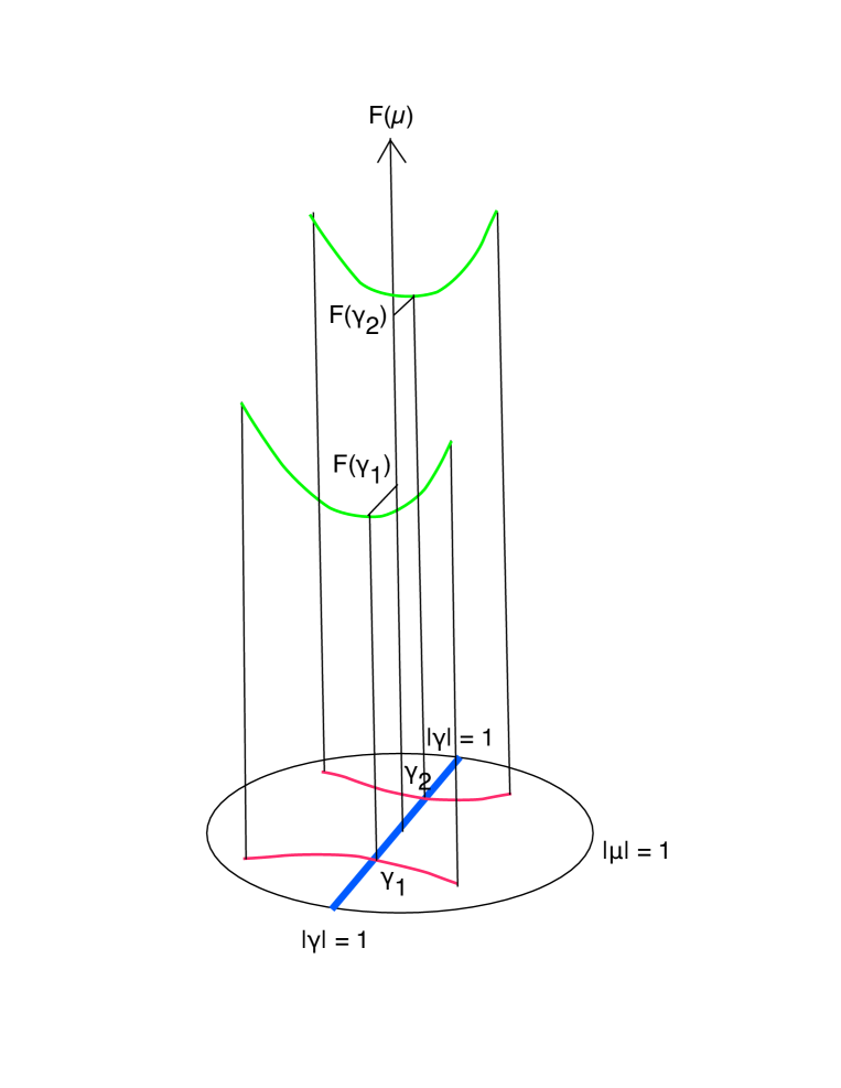
Figure 1: Plot of the values of the minimizing functional, in green, corresponding to a single gauge orbit, in red, of which only two (out of an infinite number of) disconnected branches are shown. The blue horizontal line is the Teichmüller space.

This situation is pictured in Fig. 1. The infinite-dimensional space of the $\mu(z,\bar{z})$ is represented in perspective in the horizontal plane. It contains the Teichmüller space represented by the horizontal blue line segment. A single gauge orbit, consists of an infinite number of disconnected branches, of which only two are shown in the figure. They are represented by the two disconnected horizontal red curves that intersect the Teichmüller space at $\mu=\gamma_{1}$ and $\mu=\gamma_{2}$. The Teichmüller parameters $\gamma_{!}$ and $\gamma_{2}$ are related by a ‘large’ gauge transformation $\in SL(2,Z)$. Each red curve is related to $\gamma_{1}$ or $\gamma_{2}$ by a ‘small’ gauge transformation that is continuously connected to the identity. The vertical axis measures values of the minimizing functional $F(\mu)$, and the two green curves show the values of $F(\mu)$ for points $\mu$ on the gauge orbit, just described, that is obtained from the green curves by vertical projection. The green curves are at a minimum at $F(\gamma_{1})$ and $F(\gamma_{2})$, where the branches of the gauge orbit intersect the Teichmüller space.

An interesting feature is that there can be only a single minimum of the minimizing functional on each connected branch of a gauge orbit. Indeed, suppose that there were two relative minima on the same branch. In this case they are related by a gauge transformation that is continuously connected to the identity. On the other hand each minimum satisfies the stationarity condition, which means that each minimum is a point in the Teichmüller space. However, within the Teichmüller space, two points that are gauge-equivalent are related by a large diffeomorphism, which cannot be continuously connected to the identity. Thus we have arrived at a contradiction, which shows that there cam be only a single minimum on each connected branch of a gauge orbit. We shall show explicitly for the case of the torus that the single minimum does in fact exist for appropriately chosen minimalising functional.

6 BRST-invariant action

We would like to impose the above gauge fixing in a BRST-invariant way. For this purpose, we introduce the gauge-fixing BRST-exact Lagrangian,

$$s\int dzd{\bar{z}}[b_{zz}(\mu^{z}_{\bar{z}}-{\mu^{z}_{\bar{z}}}_{0})+c.c.] = \int dzd{\bar{z}}\Big{(}\lambda_{zz}(\mu^{z}_{\bar{z}}-{\mu^{\bar{z}}_{z}}_{0})-b_{zz}(\partial_{\bar{z}}c^{z}+c^{z}\partial_{z}\mu^{z}_{\bar{z}}-\mu^{z}_{\bar{z}}\partial_{z}c^{z})\Big{)}$$ (25)

$$+ \sum_{1\leq i\leq 3g-3}l^{i}\int dzd{\bar{z}}\frac{\partial{\mu^{z}_{\bar{z}}}_{0}(\gamma,\bar{\gamma},z,{\bar{z}})}{\partial\gamma^{i}}b_{zz}+c.c.,$$

where the BRST-operator $s$ acts according to

$$s\mu^{z}_{\bar{z}} = \partial_{\bar{z}}c^{z}+c^{z}\partial_{z}\mu^{z}_{\bar{z}}-\mu^{z}_{\bar{z}}\partial_{z}c^{z}\ \ \ \ \ \ \ \ \ \ sc^{z}=c^{z}\partial_{z}c^{z}$$

$$sb_{zz} = \lambda_{zz}\ \ \ \ \ \ \ \ \ \ \ \ \ \ \ \ \ \ \ \ \ \ \ \ \ \ \ \ \ \ \ \ \ \ \ \ \ s\lambda_{zz}=0$$

$$s\gamma^{i} = l^{i}\ \ \ \ \ \ \ \ \ \ \ \ \ \ \ \ \ \ \ \ \ \ \ \ \ \ \ \ \ \ \ \ \ \ \ \ \ \ \ \ \ sl^{i}=0,$$ (26)

and c.c., with $s^{2}=0$. Here the $\gamma$ are in a fundamental domain containing the value $\gamma=0$. The Lagrange multiplier $\lambda_{zz}$ assures that the minimization condition on $\mu^{z}_{\bar{z}}$ is satisfied on each gauge orbit, and this value of $\mu^{z}_{\bar{z}}$ automatically gets substituted everywhere in the action and the observables.

The last term in the action imposes, by integration over the $l^{i}$, that the antighost field $b$ remains orthogonal to all zero modes in the Fadeev–Popov operator, defined by $(\partial_{\bar{z}}-\mu^{z}_{\bar{z}}\partial_{z}+2\partial_{z}\mu^{z}_{\bar{z}})b_{zz}=0$.

We will check that no zero eigenvalue occurs for the torus, by an appropriate choice of the function $f$. In fact the zero mode occurs only at the singular part of the boundary of the minimizing fundamental domain, which constitutes therefore a harmless Gribov horizon.

The definition of the observables as $s$-invariant quantities that are not $s$-exact ensures that they cannot depend on the $\gamma$’s, because the pairs $(\gamma,l)$ are BRST-trivial doublets. Their field dependance is only though the string field $X$ and the Beltrami differentials $\mu^{z}_{\bar{z}}$ and $\mu^{\bar{z}}_{z}$ (and their supersymmetric partners in the superstring case).

The alternative of imposing equations (18) as gauge conditions, by means of Lagrange multiplier fields in a standard BRST-invariant way will be sketched in an Appendix. However this gauge choice is impractical because gravitational degrees of freedom propagate, and for this reason we shall impose instead the solution of this equation, which is $\mu_{\overline{z}}^{z}=\gamma$ in the case of the torus.

7 The case of the torus

7.1 Identification of the domain that minimizes the gauge-functional

For the torus, the Teichmüller space can be represented as the upper half-plane of complex $\tau$, with $Im(\tau)\geq 0$. Two points that differ by any given $SL(2,Z)$ transformation

$$\tau\to\frac{a\tau+b}{c\tau+d},$$ (27)

where $a,b,c$ and $d$ are positive or negative integers, represents the same torus. These transformations can be decomposed as successions of transformations

$$\tau\to\frac{-1}{\tau};\ \ \ \ \ \ \ \tau\to{\tau+1}.$$ (28)

As is well known, the first fundamental domain is defined by $-\frac{1}{2}\leq Re(\tau)\leq\frac{1}{2}$ and $\tau\bar{\tau}\geq 1$. All other fundamental domains are obtained from compositions of transformations (28).

For any given Riemann surface one has everywhere $|\mu^{z}_{\bar{z}}|<1$. It is thus appropriate to redefine the Teichmüller parameters in such a way that they are confined in a disk where their modulus remains smaller than one. For the torus, the solution is obvious; all points of the complex upper-half plane Im$\ \tau\geq 0$ are mapped onto the Poincaré disk $\cal D$, $|\gamma|\leq 1$, by

$$\gamma=\frac{\tau-i}{\tau+i}$$ (29)

As we will show, this opens the way to the gauge-fixing of 2d-gravity in a very simple way.

Figure 2 shows the image $\cal D_{I}$ of the first fundamental domain for the case of the torus. The mapping $\tau\to\frac{-1}{\tau}$ corresponds to a symmetry $\gamma\to-\gamma$ for every point of any given fundamental domain. The mapping $\tau\to{\tau+n}$ sends a point $\gamma$ of the domain $I$ into a point $\gamma_{n}$ of another fundamental domain such that $\gamma_{n}>\gamma$.

The curves in $\gamma$-space that appear in the figure are found from the inversion,

$$\tau=i\Big{(}{1+\gamma\over 1-\gamma}\Big{)}=i\Big{(}{1+x+iy\over 1-x-iy}\Big{)},$$ (30)

where we have separated $\gamma$ into its real and imaginary parts. One easily finds that the boundary of the Teichmüller space, ${Im}(\tau)=0$ corresponds in the $\gamma$ plane to the unit circle $x^{2}+y^{2}=1$, whereas the boundary of the first fundamental modular region, made up of parts of the curves ${Re}(\tau)=\pm 1/2$, and $|\tau|=1$, is made up in the $\gamma$ plane by parts of the curves $(x-1)^{2}+(y\mp 2)^{2}=2^{2}$ and $x=0$, as drawn in Fig. 2.

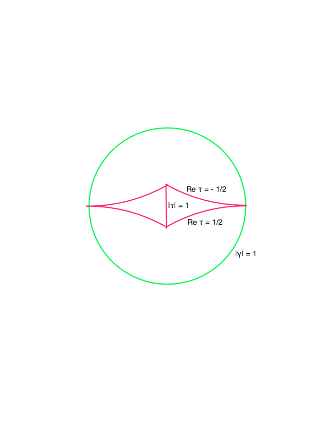
Figure 2: The Poincaré disk $|\gamma|\leq 1$ corresponds to the Teichmüller space ${\rm Im}\tau\geq 0$. The first fundamental modular region of the torus, and its copy under $\gamma\to-\gamma$, are outlined in red, as the interior of both adjacent triangles in the middle of the $\gamma$ plane. For these domains, the point $|\gamma|=0$ is the representative of the “squared” torus. This point can be e.g. chosen as the reference point for the minimizing functional in string theory. All other fundamental domains are obtained by modular transformations. Each one of them intersects only once the boundary circle $|\gamma|=1$. On the other hand any given point of this boundary belongs to several fundamental domains. The boundary of the Poincaré disk can be therefore named as the (harmless) horizon of 2-dimensional gravity.

7.2 BRST-invariant representation of the minimizing domain

For genus $g=1$, the last Lagrangian simplifies to

$$s(\int dzd\bar{z}\Big{(}b_{zz}(\mu^{z}_{\bar{z}}-\gamma)\Big{)}=\int dzd\bar{z}\Big{(}\lambda_{zz}(\mu^{z}_{\bar{z}}-\gamma)-b_{zz}(\partial_{\bar{z}}c^{z}-\gamma\partial_{z}c^{z})\Big{)}+l\int dzd\bar{z}\ b_{zz}$$

$$+c.c.,\ \ \ \ \ \ \ \ \ \ \ \ \ \ \ \ \ \ \ \ \ \ \ \ \ \ \ \ \ \ \ \ \ \ \$$ (31)

where $s$ acts as in (6). This expression must be added to the Polyakov action, which is BRST-invariant but not BRST-exact. The gauge-fixing action (7.2) identifies $\lambda_{zz}$, as a Lagrange multiplier field for $\mu^{z}_{\bar{z}}$. The constant fermionic Lagrange multiplier $l$ imposes that the zero mode of the operator $\partial_{\bar{z}}-\gamma\partial_{z}$ is omitted. Consequently the ghost and anti-ghost integrations give a regularised determinant, $\det^{\prime}(\partial_{\bar{z}}-\gamma)$. Eventually, the integration over $\gamma$ must be done over the fundamental domain that we found by our minimizing principal for each orbit. This reproduces the known result for the partition function of string theory with a 1-torus worldsheet. In this construction, it must be noted that, although one has escaped the consequence of Singer’s theorem by solving a minimizing principle, a BRST symmetry has been preserved all along the way, allowing one to prove by locality properties that the observables satisfy all requirements concerning factorization and modular invariance. Notice that the degenerate point $\gamma=1$ is safely approached. This is where the torus approaches the pinched torus, that is, a sphere with two identified points. If an observable produces divergences as one approaches this point, one must e. g. use a cutoff $|\gamma|<1-\epsilon$, consistent with the BRST Ward identity (see the previous section), so the divergence cancels in the limit $\epsilon\to 0$.

We now verify the absence of zero modes of the second variation of the minimizing functional, except at the singular point $|\gamma|=1$, and we determine the criteria on the function $f$ in order that the second variation of the minimizing functional $F$ be strictly positive for $\gamma<1$.

7.2.1 Eigenvalues and zero modes of the Faddeev-Popov operator

We shall calculate the eigenvalues of the Faddeev-Popov operator

$$M\equiv\overline{\partial}-\gamma\partial$$ (32)

where $\partial\equiv{\partial\over\partial z}$ and $\overline{\partial}\equiv{\partial\over\partial\overline{z}}$.

This operator acts on functions $f(z,\overline{z})$ that are doubly periodic in the basic parallelogram

$$f(x+1,y)=f(x,y+1)=f(x,y).$$ (33)

where $z=x+iy$, and $x$ and $y$ are real. Note that the boundary conditions satisfied by the coordinates are fixed, independent of the metric, because our transformations are all active, that is to say, they act on the fields only.

The Faddeev-Popov operator is a derivative with constant coefficients which is diagonalized by an exponential,

$$f_{m,n}(x,y)=\exp[2\pi i(mx+ny)],$$ (34)

and the boundary conditions are satisfied by taking $m$ and $n$ to be integers. Thus the general solution with the doubly periodic boundary conditions reads, in terms of $z$ and $\overline{z}$

$$f_{m,n}(x,y)=\exp[\pi(mi+n)z+\pi(mi-n)\overline{z}].$$ (35)

The eigenvalues of the Faddeev-Popov operator are obtained from

$$(\overline{\partial}-\gamma\partial)f_{m,n}=E_{m,n}f_{m,n},$$ (36)

which gives

$$E_{m,n}=\pi(mi-n)-\gamma\pi(mi+n).$$ (37)

The null eigenvalues satisfy $E_{m,n}=0$, which gives for the values of $\gamma$ that correspond to null eigenvalues,

$$\gamma=-{n-mi\over n+mi}.$$ (38)

This implies

$$|\gamma|=1,$$ (39)

and so all values of $\gamma$ that correspond to zero-modes of the Faddeev-Popov operator $M=\overline{\partial}-\gamma\partial$ lie on the unit circle.

7.2.2 Second variation of minimizing functional

The derivation of the second variation of $F$ is simplified by never partially integrating on $\mu$ or $\bar{\mu}$ because, in the end, the condition of minimisation that is imposed, is $\mu^{z}_{\bar{z}}=\gamma$ = const. For notational simplicity we now set $\mu=\mu^{z}_{\bar{z}}$ and $\bar{\mu}=\mu^{\bar{z}}_{z}$.

The minimizing functional is given by

$$F=\int d^{2}z\ \rho\ f(\bar{\mu}\mu).$$ (40)

Its first variation is

$$\delta F = \int d^{2}z\ \rho\ f^{\prime}(\bar{\mu}\mu)\ (\delta\bar{\mu}\mu+\bar{\mu}\delta\mu)$$ (41)

$$= \int d^{2}z\ \rho\ f^{\prime}(\bar{\mu}\mu)\ (\nabla\bar{\epsilon}\mu+\bar{\mu}\overline{\nabla}\epsilon),$$

where we have used

$$\delta\mu=\overline{\nabla}\epsilon\equiv(\bar{\partial}-\mu\partial+\partial\mu)\epsilon,$$ (42)

and cc.

The second variation is then

$$\delta^{2}F = \int d^{2}z\ \rho\ \{\ f^{\prime\prime}(\bar{\mu}\mu)\ (\nabla\bar{\epsilon}\mu+\bar{\mu}\overline{\nabla}\epsilon)^{2}$$ (43)

$$\ \ \ \ \ \ \ \ \ \ \ +\ f^{\prime}(\bar{\mu}\mu)\ [\ 2\nabla\bar{\epsilon}\overline{\nabla}\epsilon+\delta(\nabla\bar{\epsilon})\mu+\bar{\mu}\delta(\overline{\nabla}\epsilon)\ ]\ \}.$$

By (42) we have $\delta\overline{\nabla}\epsilon=(-\delta\mu\partial+\partial\delta\mu)\epsilon$, which gives

$$\delta\overline{\nabla}\epsilon=-\overline{\nabla}\epsilon\partial\epsilon+\partial(\overline{\nabla}\epsilon)\epsilon$$ (44)

and cc, and we have

$$\delta^{2}F = \int d^{2}z\ \rho\ \Big{[}\ f^{\prime\prime}(\bar{\mu}\mu)\ (\nabla\bar{\epsilon}\mu+\bar{\mu}\overline{\nabla}\epsilon)^{2}$$

$$\ \ \ \ \ \ \ \ \ \ \ +\ f^{\prime}(\bar{\mu}\mu)\ \Big{(}\ 2\nabla\bar{\epsilon}\overline{\nabla}\epsilon+[-\nabla\bar{\epsilon}\bar{\partial}\bar{\epsilon}+\bar{\partial}(\nabla\bar{\epsilon})\bar{\epsilon}]\mu+\bar{\mu}[-\overline{\nabla}\epsilon\partial\epsilon+\partial(\overline{\nabla}\epsilon)\epsilon]\ \Big{)}\ \Big{]}.$$

We are interested in the second variation at the stationary points of the minimizing functional, and we specialize to the torus. In this case we have $\rho=1$, and $\mu=\gamma$ and $\bar{\mu}=\bar{\gamma}$, where $\gamma$ and $\bar{\gamma}$ are complex conjugate constants with $\gamma\bar{\gamma}\leq 1$. In this case $\overline{\nabla}\epsilon$ simplifies to

$$\overline{\nabla}\epsilon\equiv(\bar{\partial}-\gamma\partial)\epsilon,$$ (46)

and cc, and we have

$$\delta^{2}F|_{\mu=\gamma} = \int d^{2}z\ \Big{[}\ f^{\prime\prime}(\bar{\gamma}\gamma)\ (\nabla\bar{\epsilon}\gamma+\bar{\gamma}\overline{\nabla}\epsilon)^{2}$$

$$\ \ \ \ \ \ \ \ \ \ \ +\ f^{\prime}(\bar{\gamma}\gamma)\ \Big{(}\ 2\nabla\bar{\epsilon}\overline{\nabla}\epsilon+[-\nabla\bar{\epsilon}\bar{\partial}\bar{\epsilon}+\bar{\partial}(\nabla\bar{\epsilon})\bar{\epsilon}]\gamma+\bar{\gamma}[-\overline{\nabla}\epsilon\partial\epsilon+\partial(\overline{\nabla}\epsilon)\epsilon]\ \Big{)}\ \Big{]}.$$

We simplify this expression by doing a partial integration in the last two terms,

$$\delta^{2}F|_{\mu=\gamma} = \int d^{2}z\ [\ f^{\prime\prime}(\bar{\gamma}\gamma)\ (\nabla\bar{\epsilon}\gamma+\bar{\gamma}\overline{\nabla}\epsilon)^{2}$$ (48)

$$\ \ \ \ \ \ \ \ \ \ \ +\ 2f^{\prime}(\bar{\gamma}\gamma)\ (\nabla\bar{\epsilon}\overline{\nabla}\epsilon-\nabla\bar{\epsilon}\bar{\partial}\bar{\epsilon}\gamma-\bar{\gamma}\overline{\nabla}\epsilon\partial\epsilon)\ ].$$

7.2.3 Positivity of eigenvalues

We wish to determine if the second variation, $\delta^{2}F|_{\mu=\gamma}$, is a positive quadratic form. Since it involves derivatives with constant coefficients, we may diagonalize it by fourier components. With coordinates $z=x+iy$ and $\bar{z}=x-iy$, the boundary conditions for the torus are

$$\epsilon(x+1,y)=\epsilon(x,y+1)=\epsilon(x,y).$$ (49)

and cc. The second variation is diagonalized by

$$\epsilon(x,y)=\alpha\sin[2\pi(mx+ny)]+\beta\cos[2\pi(mx+ny)],$$ (50)

and cc, where $m$ and $n$ are integers, and $\alpha$ and $\beta$ are complex constants. Since $\delta^{2}F|_{\mu=\gamma}$ is quadratic in the derivatives $\partial\epsilon,\partial\bar{\epsilon},\bar{\partial}\epsilon,\bar{\partial}\bar{\epsilon}$, the terms in $\sin[2\pi(mx+ny)]$ and $\cos[2\pi(mx+ny)]$, do not mix, so the terms in $\alpha$ and $\beta$ do not mix, and we may diagonalize by taking $\beta=0$ or $\alpha=0$. These choices give the same result, and we take

$$\epsilon(x,y) = \alpha\sin[2\pi(mx+ny)]$$

$$\bar{\epsilon}(x,y) = \bar{\alpha}\sin[2\pi(mx+ny)]$$ (51)

We have

$$\partial=\partial_{z}=(1/2)(\partial_{x}-i\partial_{y})$$

$$\bar{\partial}=\partial_{\bar{z}}=(1/2)(\partial_{x}+i\partial_{y}),$$ (52)

which gives

$$\partial\epsilon=\overline{W}\alpha\cos[2\pi(mx+ny)];\ \ \ \ \partial\bar{\epsilon}=\overline{W}\bar{\alpha}\cos[2\pi(mx+ny)]$$

$$\bar{\partial}\epsilon=W\alpha\cos[2\pi(mx+ny)];\ \ \ \ \bar{\partial}\bar{\epsilon}=W\bar{\alpha}\cos[2\pi(mx+ny)]$$ (53)

and

$$\overline{\nabla}\epsilon=V\alpha\cos[2\pi(mx+ny)]$$

$$\nabla\bar{\epsilon}=\overline{V}\bar{\alpha}\cos[2\pi(mx+ny)],$$ (54)

where

$$W\equiv\pi(m+in);\ \ \ \ \ \ \overline{W}\equiv\pi(m-im).$$ (55)

and

$$V \equiv W-\gamma\overline{W}$$

$$\overline{V} \equiv \overline{W}-\bar{\gamma}W.$$ (56)

Upon integrating over $x$ and $y$, we obtain for the second variation

$$2\delta^{2}F|_{\mu=\gamma}=f^{\prime\prime}(\overline{V}\gamma\bar{\alpha}+V\bar{\gamma}\alpha)^{2}+2f^{\prime}(|V|^{2}\bar{\alpha}\alpha-V\overline{W}\bar{\gamma}\alpha^{2}-\overline{V}W\gamma\bar{\alpha}^{2}).$$ (57)

In terms of the variables $\alpha$ and $\bar{\alpha}$, this is the quadratic form

$$2\delta^{2}F|_{\mu=\gamma}=A\bar{\alpha}\alpha+B\alpha^{2}+\overline{B}\bar{\alpha}^{2},$$ (58)

where

$$A\equiv 2f^{\prime\prime}|V|^{2}\bar{\gamma}\gamma+2f^{\prime}|V|^{2}$$ (59)

$$B\equiv f^{\prime\prime}V^{2}\bar{\gamma}^{2}-2f^{\prime}V\overline{W}\bar{\gamma},$$ (60)

and cc. In terms of the real variables

$$\alpha=r+is;\ \ \ \ \ \bar{\alpha}=r-is$$ (61)

it reads

$$2\delta^{2}F|_{\mu=\gamma}=(A+B+\bar{B})r^{2}+(A-B-\bar{B})s^{2}+2i(B-\bar{B})rs.$$ (62)

The eigenvalues of this real quadratic form are easily found to be

$$\lambda=A\pm 2\bar{B}B.$$ (63)

For appropriately chosen $f(x)$, the derivatives $f^{\prime}(x)$ and $f^{\prime\prime}(x)$ are positive, so $A$ is positive, and both roots will be positive if $A^{2}>4\bar{B}B$ namely, if

$$A^{2}-4\bar{B}B>0.$$ (64)

We wish to determine if this quantity is positive for all values of $W$ and $\gamma$, with $\bar{\gamma}\gamma\leq 1$.

To simplify the calculation we write

$$V=Wv;\ \ \ \ \ \overline{V}=\overline{W}\bar{v}$$ (65)

where, by (7.2.3),

$$v\equiv 1-\sigma;\ \ \ \ \ \ \bar{v}=1-\bar{\sigma}$$ (66)

and

$$\sigma\equiv\gamma{\overline{W}\over W}=|\gamma|e^{i\phi};\ \ \ \ \ \ \bar{\sigma}\equiv\bar{\gamma}{W\over\overline{W}}=|\gamma|e^{-i\phi}.$$ (67)

Here $\phi$ is a pure phase because

$${\overline{W}\over W}={m-in\over m+in},$$ (68)

is a pure phase, and we have

$$\bar{\sigma}\sigma=\bar{\gamma}\gamma.$$ (69)

In terms of these variables we have

$$A = 2f^{\prime}|V||W||v|(R|\gamma|^{2}+1)$$

$$B = f^{\prime}V\overline{W}\bar{\gamma}(Rv\bar{\sigma}-2)$$

$$\overline{B} = f^{\prime}\overline{V}W\gamma(R\bar{v}\sigma-2),$$ (70)

where we have introduced the ratio of derivatives

$$R\equiv{f^{\prime\prime}(\bar{\gamma}\gamma)\over f^{\prime}(\bar{\gamma}\gamma)}.$$ (71)

Positivity of the second variation is determined by the positivity of

$$Q\equiv{A^{2}-4\overline{B}B\over 4|V|^{2}|W|^{2}f^{\prime 2}}.$$ (72)

which is given by

$$Q = |v|^{2}(R|\gamma|^{2}+1)^{2}-|\gamma|^{2}(R\bar{v}\sigma-2)(Rv\bar{\sigma}-2)$$ (73)

$$= 2R|\gamma|^{2}\ (\ |v|^{2}+v\bar{\sigma}+\overline{v}\sigma\ )+\ |v|^{2}-4|\gamma|^{2},$$

where the term in $R^{2}$ has cancelled because $|\sigma|^{2}=|\gamma|^{2}$.

To evaluate this expression, we use $v=1-\sigma$, which gives

$$|v|^{2}=(1-\sigma)(1-\bar{\sigma})=1-\sigma-\bar{\sigma}+|\gamma|^{2}$$ (74)

$$v\bar{\sigma}+\overline{v}\sigma=(1-\sigma)\bar{\sigma}+(1-\bar{\sigma})\sigma=\sigma+\bar{\sigma}-2|\gamma|^{2},$$ (75)

so

$$|v|^{2}+v\bar{\sigma}+\bar{v}\sigma=1-|\gamma|^{2},$$ (76)

and we obtain

$$Q=2R|\gamma|^{2}(1-|\gamma|^{2})+1-2|\gamma|\cos\phi+|\gamma|^{2}-4|\gamma|^{2},$$ (77)

where we have used $\sigma+\bar{\sigma}=2|\gamma|\cos\phi$. This expression is a minimum at $\cos\phi=1$, so $Q$ will be positive for all $m$ and $n$ if and only if $Q$ is positive at this minimum, namely if

$$Q_{\rm min}\equiv 2R|\gamma|^{2}(1-|\gamma|^{2})+(1-|\gamma|)^{2}-4|\gamma|^{2}$$ (78)

is positive. For $|\gamma|$ close to 1, all terms are small except the last one — which is negative — unless we can save the day by an appropriate choice of $f(|\gamma|^{2})$. Indeed let us choose

$$f(x)={1\over(1-x)^{p}},$$ (79)

where $p$ is a power at our disposal. We have

$$R(x)={f^{\prime\prime}(x)\over f^{\prime}(x)}={p+1\over 1-x}$$ (80)

and, with $x=|\gamma|^{2}$, we obtain

$$Q_{\rm min}=2(p+1)|\gamma|^{2}+(1-|\gamma|)^{2}-4|\gamma|^{2}$$

$$=2(p-1)|\gamma|^{2}+(1-|\gamma|)^{2}.$$ (81)

This will be positive for all $|\gamma|\leq 1$ if and only if $p\geq 1$. Thus for $f(x)$ of the form (79), $Q$ is non-negative for all $|\gamma|\leq 1$ and all integers $m$ and $n$ provided that

$$p\geq 1.$$ (82)

This is necessary and sufficient for $\delta^{2}F$ to be a positive form. Other expressions for $f(x)$ will also satisfy this condition, but they must have the singularity at $|\gamma|=1$ of the strength found here. For example $f(x)=-\ln(1-x)$ will not do, and with the simplest choice $F=\int dzd{\bar{z}}\ \mu\bar{\mu}$, one would gets a negative eigenvalue for $|\gamma|>1/3$.

The condition

$$Q_{\rm min}\geq 0,$$ (83)

where $Q_{\rm min}$ is defined in (78) provides a simple criterion which determines whether the second variation of the minimizing functional $\delta^{2}F$ is a positive form or not.

8 Definiteness and convergence of the gauge-fixing process through stochastic quantization

Stochastic quantization materializes quantum fluctuation by a Langevin equation, with a Gaussian noise $b$ and a drift force that is equal to the sum of the classical equation of motion, $-{\delta S\over\delta\phi}$ and a “force”, $\delta_{v}(\phi)$, tangent to the gauge orbit, that is given by a gauge transformation (in our case a reparametrization) with a field-dependent generator $v^{z}$. The latter must be chosen in such a way that the Langevin process converges at infinite values of a stochastic time $t$, and the Langevin equation for any given field reads, in general

$$\partial_{t}\phi=-\frac{\delta S}{\delta\phi}^{\rm classical}+\delta_{{\rm gauge},v}(\phi)+b_{\phi}(x,t),$$ (84)

where $b_{\phi}(x,t)$ is a white noise for $\phi(x,t)$. The correlation functions of gauge independent operators cannot depend on the the choice of $v$ (provided the stochastic process is well defined).

In the case of 2d-gravity, the last equation remains formal because in order to achieve the condition $|\mu^{z}_{\bar{z}}|<1$, one cannot assume stricto-sensu that all fluctuations of the noise $b_{\phi}(x,t)$ are allowed. This problem is possibly solved by reformulating the stochastic process under the form of Fockker–Planck equation, where the notion of a noise disappears when the Fockker–Planck kernel is introduced.

For our case, the gauge symmetry is 2d-reparametrization. All fields now depend on $z,{\bar{z}},t$, and for every gauge orbit, we introduce the following metric dependent gauge function

$$v^{z}=\rho^{z{\bar{z}}}f^{\prime}\nabla^{(\mu^{\bar{z}}_{z})}_{z}\mu^{z}_{\bar{z}}$$ (85)

Call $b_{\mu^{z}_{\bar{z}}}$ and $b_{X}$ Gaussian noises for ${\mu^{z}_{\bar{z}}}$ and $X$. Both Langevin equations for the Beltrami differential and the string field are

$$\partial_{t}\mu^{z}_{\bar{z}}=T_{zz}-\nabla_{\bar{z}}(\rho^{z{\bar{z}}}f^{\prime}\nabla^{(\mu^{\bar{z}}_{z})}_{z}\mu^{z}_{\bar{z}})+b_{\mu^{z}_{\bar{z}}}$$ (86)

where $T_{zz}$ is the classical energy momentum tensor

$$T_{zz}=\frac{\delta S}{\delta\mu^{z}_{\bar{z}}}^{\rm Polyakov}=\frac{\partial_{\bar{z}}-\mu^{z}_{\bar{z}}\partial_{z}}{1-\mu^{z}_{\bar{z}}\mu^{\bar{z}}_{z}}X\cdot\frac{\partial_{\bar{z}}-\mu^{z}_{\bar{z}}\partial_{z}}{1-\mu^{z}_{\bar{z}}\mu^{\bar{z}}_{z}}X$$ (87)

and

$$\partial_{t}X=-(\nabla_{\bar{z}}\nabla_{z}+\nabla_{z}\nabla_{\bar{z}})X+\rho^{z{\bar{z}}}f^{\prime}\nabla^{(\mu^{\bar{z}}_{z})}_{z}\mu^{z}_{\bar{z}}\nabla_{z}X+\rho^{z{\bar{z}}}f^{\prime}\nabla^{(\mu^{z}_{\bar{z}})}_{\bar{z}}\mu^{\bar{z}}_{z}\nabla_{\bar{z}}X+b_{X}$$ (88)

The presence of a Laplacian with no zero modes in both equations ensures a well-defined converging stochastic process, and the gauge-fixing is well-achieved in this method. To implement the form of the explicit equilibrium Fokker–Planck distribution of the Langevin process is probably an impossible task, since both Langevin equations involve nontrivial gravitational interactions between the $\mu^{z}_{\bar{z}}$ and $X$ fields having explicitly no zero-mode problems in the stochastic process, but a ghost-free field theory has a price, namely the existence of of gravitational interactions.

The role of the functions $\ln\rho_{z{\bar{z}}}(z,{\bar{z}})$ and $f$ in the definition of the drift force along the gauge orbit is to ensure that the latter is always a restoring one, and that it can vanish only at the boundary of a fundamental domain. If these functions are not well chosen, an artificial singularity of the Langevin/Fokker–Planck process may occur, where the drift force can change sign, but this just an artifact of a bad system of coordinates, which is analogous to the (pseudo) Schwartzschild singularity in the description of a black hole.

9 Conclusion

This paper high-lights the property that the Gribov question is not a problem in string theory. There is an unambiguous gauge-fixing, with a minimizing principle on each orbit, such that the Faddeev-Popov determinant in a BRST-invariant description cannot possibly change sign in a fundamental domain. Infrared problems may occur for certain modular invariant observables, when the moduli approaches the singular points of the fundamental domain. Their existence is certain, since a multitorus of genus $g$ can be pinched in a number of ways, and can be identified as a Riemann surface of lower genus with identified points, a geometrical feature that seems to be the origin of possible IR divergencies of the field theory limit of string theory.

The method indicates that a complete knowledge of the moduli space of Riemann surfaces is necessary to get a reliable BRST-invariant action for the theory. Since the method has a straightforward generalization for the superstring, we left aside the tachyon problem, which is irrelevant for the question of gauge-fixing.

The string is thus a very interesting laboratory for gauge-fixing questions. Choosing an absolute minimum for a gauge-fixing functional on each orbit selects a unique representative of the worldsheet metric, orbit per orbit. This choice can be enforced in a BRST-invariant way. It allows one to select and compute all observables of the theory, while respecting all BRST Ward identities. The expressions found are given by the usual integrals over a fundamental domain of Riemann surfaces, at a fixed genus.

This fundamental domain is in fact found by minimizing a certain distance in the space of Beltrami differentials, which corresponds to the gauge-fixing functional on each orbit.

In the case of the torus one can explicitly verify that no Gribov issue arises. A horizon exists however, and is found to be the boundary of the Poincaré disk, where the quantum-field-theory limit of string theory is defined. This boundary of the Teichmüller space is degenerate, in the sense that it represents a surface for which the absolute minimum of the gauge-fixing functional is degenerate. It gathers all the singular points of the boundaries of each fundamental domain, when the torus becomes degenerate, as a sphere with a pair of points identified (pinched torus). However, when one restricts to one given fundamental domain, only one of these points occurs, and its contribution can safely regularised, provided one computes infra-red safe observables.

Acknowledgements : We thank L. Alvarez-Gaume, S. Cappell, M. Douglas, S. Grushevsky, E. Y. Miller, N. Nekrasov, I.M. Singer and L. Takhtajan for very interesting discussions. We are grateful to M. Porrati and R. Stora for many valuable and informative conversations.

10 Appendix A : Sketch of the condition $\nabla_{\bar{z}}h_{zz}$ in a standard BRST construction

In this section, for the sake of curiosity, we show an attempt to directly enforce the minimizing gauge-condition $\nabla_{\bar{z}}h_{zz}$ in the “standard” BRST construction, as one does in the perturbative Yang–Mills landau gauge. For this purpose, one uses a Lagrange multiplier local field $\lambda_{z}$ for imposing the condition by adding to the action a term $\int d^{2}z\lambda_{z}\nabla_{z}\mu^{z}_{\bar{z}}$. To make this term part of a BRST-exact term, one also introduces an anti-ghost field $C_{z}$, such that $sC_{z}=\Lambda_{z}$. One does the analogous for the other sector.

The anti-ghost $C_{z}$ cannot have generic zero modes, since it has a single holomorphic index, like the Faddeev Popov ghost $c^{z}$, but the existence of the 3g-3 global zero modes will pop up in a different manner as for the antighost $b_{zz}$ of the previous method. These zero modes will be carried by the now propagating Beltrami differential, and a deficit between the number of propagating zero modes of the Beltrami differential and the Lagrange multipliers. The theory seems in fact almost impossible to solve, since we will get a theory where the 2d-gravity fields become propagating, apparently like the longitudinal gluon in the Yang–Mills theory in the Landau gauge.

According to the “naive” idea of BRST quantization, we thus tentatively define the BRST gauge-fixing action action as

$$\int d^{2}z\ s\Big{(}C^{z}(\partial_{\bar{z}}-\mu^{z}_{\bar{z}}\partial_{z}-2\partial_{z}\mu^{z}_{\bar{z}})f^{\prime}\rho_{z{\bar{z}}}\mu^{\bar{z}}_{z}+s(C^{\bar{z}}(\partial_{z}-\mu^{\bar{z}}_{z}\partial_{\bar{z}}-2\partial_{\bar{z}}\mu^{\bar{z}}_{z})f^{\prime}\rho_{z{\bar{z}}}\mu^{z}_{\bar{z}}\Big{)}$$

$$=\int d^{2}z\ s(C_{\bar{z}}\nabla_{\bar{z}}f^{\prime}\rho_{z{\bar{z}}}\mu^{\bar{z}}_{z}+C_{z}\nabla_{z}f^{\prime}\rho_{z{\bar{z}}}\mu^{z}_{\bar{z}})\ \ \ \ \ \ \ \ \ \ \ \ \ \ \$$ (89)

that is,

$$\int d^{2}z\ (\Lambda^{z}\nabla_{\bar{z}}f^{\prime}\rho_{z{\bar{z}}}\mu^{\bar{z}}_{z}+\Lambda^{\bar{z}}\nabla_{z}f^{\prime}\rho_{z{\bar{z}}}\mu^{z}_{\bar{z}}-\begin{pmatrix}C^{z}&C^{\bar{z}}\end{pmatrix}\begin{pmatrix}s(\partial_{\bar{z}}-\mu^{z}_{\bar{z}}\partial_{z}-2\partial_{z}\mu^{z}_{\bar{z}})f^{\prime}\rho_{z{\bar{z}}}\mu^{\bar{z}}_{z}\\ s(\partial_{z}-\mu^{\bar{z}}_{z}\partial_{\bar{z}}-2\partial_{\bar{z}}\mu^{\bar{z}}_{z})f^{\prime}\rho_{z{\bar{z}}}\mu^{z}_{\bar{z}}\end{pmatrix}$$

This action is problematic. The ghost terms are probably well defined by a proper choice of the function $f^{\prime}$. However, one has global zero modes for $f^{\prime}\rho_{z{\bar{z}}}\mu^{z}_{\bar{z}}$ and $f^{\prime}\rho_{z{\bar{z}}}\mu^{\bar{z}}_{z}$. One must force $f^{\prime}\rho\mu$ to remain in the appropriate space of the same dimension as $\Lambda$, by a gauge-fixing involving constant ghosts. This is probably the way an integration over a fundamental domain will make its way in the expression of the partition function. There is not much motivation to check the details because in this action the Beltrami differentials now become propagating fields, as do $\Lambda_{\bar{z}}$ and $\Lambda_{z}$, and one gets gravitational interactions with the string field $X$. We thus expect super-renormalizable 2-d quantum field theory, with a subtle infra-red problem.

One can however check the consistency of this theory by computing its conformal anomaly, which only involves the local structure of the worldsheet. This is a purely local question that can be done at genus zero. One must compute perturbatively $\nabla_{\bar{z}}T_{z}z(x),T_{z}z(y)$ and check its vanishing condition, to be able to enforce the BRST Ward identity. This computation was done a long time ago, (it was motivated by different concerns [5]). The computation with a propagating metric involves loops containing the free propagators of $\mu,\Lambda,c,C$ and $X$. The contribution of the ghosts is not the same as in the conformal gauge, due to the different conformal weights of the anti-ghosts, but one still gets the condition $D-26=0$ due to compensating contribution of internal loops of $\mu^{z}_{\bar{z}}$ and $\Lambda$.

It is important that the method we advocate of defining the gauge-fixing by the minimizing principle on each orbit is however completely well defined, since, as shown in this Appendix, the attempt to enforce the condition $\nabla f^{\prime}\rho\mu=0$ in a conventional BRST-invariant way leads to unnecessary stringy complications, such as the propagation of lagrange multipliers of the BRST symmetry, with the occurrence of extra zero modes that seem difficult to solve.

11 Appendix B: Superstring extension

For the superstring case, the Beltrami differential gets a supersymmetric partner, the conformal invariant part of the 2d gravitino, with 2 components $\alpha_{z}^{+}(z,{\bar{z}}),\alpha_{\bar{z}}^{-}(z,{\bar{z}})$. The 2d spinor $\alpha_{\bar{z}}^{+},\alpha_{z}^{-}$ is defined in the tangent plane of the Riemann surface, and its large gauge transformations are deduced from those of the Beltrami differential. Calling $\gamma^{\pm}$ the local ghost of local supersymmetry, the small reparametrization and supersymmetry gauge transformations are represented by the following BRST transformations

$$s\mu^{z}_{\bar{z}} = \partial_{\bar{z}}c^{z}+c^{z}\partial_{z}\mu^{z}_{\bar{z}}-\mu^{z}_{\bar{z}}\partial_{z}c^{z}+\alpha_{\bar{z}}^{+}\gamma^{z}$$

$$sc^{z} = c^{z}\partial_{z}c^{z}+\frac{1}{2}\gamma^{z}\gamma^{z}$$

$$s\alpha_{\bar{z}}^{+} = \partial_{\bar{z}}\gamma^{z}+\mu^{z}_{\bar{z}}\partial_{z}\gamma^{z}-\frac{1}{2}\gamma^{z}\partial_{z}\gamma^{z}+c^{z}\partial_{z}\alpha_{\bar{z}}^{+}-\frac{1}{2}\alpha_{\bar{z}}^{+}\partial_{z}c^{z}$$

$$s\gamma_{z}^{+} = c^{z}\partial_{z}\gamma_{z}^{+}-\frac{1}{2}\gamma_{z}^{+}\partial_{z}c^{z}$$ (91)

and complex conjugate equations. The question of the gauge-fixing of the local supersymmetry can be solved with the generalisation of the method we introduced for the Beltrami differential. There are gauge orbits for $\alpha_{\bar{z}}^{+}$ and $\alpha_{z}^{-}$. The choice of a unique representative both for $\mu$ and $\alpha$ will be obtained by a minimizing principle, using for instance the functional

$$F[\mu^{z}_{\bar{z}},\mu^{\bar{z}}_{z},\alpha_{z},\alpha_{\bar{z}}]=\int_{\Sigma}\rho_{z{\bar{z}}}(z,{\bar{z}})dzd{\bar{z}}\ \frac{1}{{1-|\mu(z,{\bar{z}})|^{2}}}$$ (92)

$$\Big{(}\ln\frac{1-|\mu(z,{\bar{z}})|}{1+|\mu(z,{\bar{z}})|}-\sqrt{\rho^{z{\bar{z}}}}\alpha_{\bar{z}}^{+}(z,{\bar{z}})\alpha_{z}^{-}(z,{\bar{z}})\Big{)}.$$ (93)

For instance, at genus one, the solution for the minimum is $\mu^{z}_{\bar{z}}=\gamma$ and $\alpha^{+}_{\bar{z}}=t$, where $t$ is a super-module, and for genus $g>2$, the Riemann-Roch theorem predicts the integration over 2g-2 super-modules, with a method completely analogous as the one we followed for the Beltrami differential, and an eventual partition with a BRST symmetry. In the path integral, the super-module is a Grasmann variable, and its BRST transform is a commuting constant $T$, with $st=T$. $T$ is unbounded and serves as a bosonic constant Lagrange multiplier for ensuring that the commuting antighost $\beta_{\bar{z}}^{-}$ has no zero modes.

References

- [1] A. M. Polyakov, Gauge Fields and Strings, Contemporary Concepts in Physics, Publisher CRC ; O. Alvarez, Theory of Strings with Boundaries: Fluctuations, Topology, and Quantum Geometry B216 (1983) 125; E. D’Hoker, D.H. Phong, The Geometry of String Perturbation Theory, Rev.Mod.Phys. 60 (1988) 917 and Multiloop Amplitudes for the Bosonic Polyakov String, Nucl.Phys. B269 (1986) 205; C.M. Becchi, C. Imbimbo, Gribov horizon, contact terms and Cech–De Rham cohomology in 2D topological gravity Nucl.Phys. B462 (1996) 571-599, hep-th/9510003.
- [2] V. N. Gribov, Quantization of non-abelian gauge theories, Nuclear Physics B139 (1978), 1-19; I. M. SInger, Some remarks on the Gribov ambiguity, Comm. Math. Phys. Volume 60, Number 1 (1978), 7-12.
- [3] L. Baulieu, M. Bellon, Beltrami Parametrization And String Theory, Phys. Lett. B196 (1987) 142; L. Baulieu, On the BRST structure of the closed string and superstring theory, in Non perturbative quantum field theory 1987 Cargèse Proceedings, Edited by G. ’t Hooft, A. Jaffe, G. Mac, P.K. Mitter, R. Stora. N.Y., Plenum Press, 1988, (NATO ASI, Series B: Physics, 185) 445-452, 1987, R. Stora, ”The role of locality in string quantization”, same proceedings, 433-444.
- [4] L. Baulieu, M. Bellon, BRST Symmetry For Finite Dimensional Invariances Applications To Global Zero Modes In String Theory, Phys. Lett. 202B 67, 1988. L. Baulieu and I. M. Singer, Conformally invariant gauge fixed actions for -D topological gravity, Comm. Math. Phys. Volume 135, Number 2 (1991).
- [5] L. Baulieu, W. Siegel, B. Zwiebach, New Coordinates For String Fields, Nucl. Phys. B287 93, 1987. L. Baulieu, A. Bilal, Weyl Invariance and Covariant Gauge Fixing for String Fields, Phys. Lett. 192B 339, 1987; M. Abe and N. Nakanishi, Indefiniteness of the conformal anomaly of the string theory in the harmonic gauge, Mod.Phys.Lett. A7 (1992).
- [6] A Proof That Witten’s Open String Theory Gives a Single Cover of Moduli Space B. Zwiebach, Commun. Math. Phys. 142, 193-216 ,1991; S. B. Giddings , S.C. Wolpert A Triangulation of Moduli Space from Light-Cone String Theory, Commun. Math. Phys. 109, 177-190, 1987.