Improved Concentration Bounds for Count-Sketch

We present a refined analysis of the classic Count-Sketch streaming heavy hitters algorithm [CCF02]. Count-Sketch uses $O(k\log n)$ linear measurements of a vector $x\in\mathbb{R}^{n}$ to give an estimate $\widehat{x}$ of $x$. The standard analysis shows that this estimate $\widehat{x}$ satisfies $\lVert\widehat{x}-x\rVert_{\infty}^{2}<\lVert x_{\overline{[k]}}\rVert_{2}^{2}/k$, where $x_{\overline{[k]}}$ is the vector containing all but the largest $k$ coordinates of $x$. Our main result is that most of the coordinates of $\widehat{x}$ have substantially less error than this upper bound; namely, for any $c<O(\log n)$, we show that each coordinate $i$ satisfies

$$(\widehat{x}_{i}-x_{i})^{2}<\frac{c}{\log n}\cdot\frac{||x_{\overline{[k]}}||_{2}^{2}}{k}$$

with probability $1-2^{-\Omega(c)}$, as long as the hash functions are fully independent. This subsumes the previous bound and is optimal for all $c$. Using these improved point estimates, we prove a stronger concentration result for set estimates by first analyzing the covariance matrix and then using a median-of-median-of-medians argument to bootstrap the failure probability bounds. These results also give improved results for $\ell_{2}$ recovery of exactly $k$-sparse estimates $x^{*}$ when $x$ is drawn from a distribution with suitable decay, such as a power law or lognormal.

We complement our results with simulations of Count-Sketch on a power law distribution. The empirical evidence indicates that our theoretical bounds give a precise characterization of the algorithm’s performance: the asymptotics are correct and the associated constants are small.

Our proof shows that any symmetric random variable with finite variance and positive Fourier transform concentrates around $0$ at least as well as a Gaussian. This result, which may be of independent interest, gives good concentration even when the noise does not converge to a Gaussian.

1 Introduction

The heavy hitters problem and the closely related sparse recovery problem are two of the most fundamental problems in the field of sketching and streaming algorithms [CCF02, CM06, GI10, CH10, Mut05]. The goal is to efficiently identify and estimate the $k$ largest coordinates of an $n$-dimensional vector using a linear sketch $Ax$ of $x$, where $A\in\mathbb{R}^{m\times n}$ has $m=O(k\log^{c}n)$ rows. The strongest commonly used formal guarantee for the quality of such an estimate is the $\ell_{\infty}/\ell_{2}$ guarantee: this is a bound for the estimate $\widehat{x}$ recovered from $Ax$ which is of the form

$$\lVert\widehat{x}-x\rVert_{\infty}^{2}\leq\lVert x_{\overline{[k]}}\rVert_{2}^{2}/k,$$ (1)

where $x_{\overline{[k]}}$ denotes the vector obtained from $x$ by replacing its largest $k$ coordinates with $0$.

The classic approach for this problem is the Count-Sketch algorithm of Charikar et al. [CCF02], which uses $m=O(k\log n)$ measurements and satisfies (1) with $1-1/n^{\Theta(1)}$ probability. It is simple, practical, and gives the best known theoretical performance in many settings. It also pioneered a technique—hashing with random signs and estimating using medians—that forms the basis for several subsequent works on sparse recovery [GLPS10, IPW11, HIKP12, Gan12].

Our result.

We show that, despite the popularity of Count-Sketch, its performance has not been fully characterized and understood. Specifically, we prove that the quality of the approximation $\widehat{x}$ given by Count-Sketch is better than the standard bound (1) suggests. While (1) gives a bound on the worst-case error of $\widehat{x}$, we prove that most coordinates of $\widehat{x}$ have asymptotically smaller error than this worst case.

The Count-Sketch of a vector $x$ using $R$ rows of $C$ columns is defined as follows. For $u\in[R]$, we choose hash functions $h_{u}:[n]\to[C]$ and $s_{u}:[n]\to\{\pm 1\}$. The sketch is

$$y_{u,v}=\sum_{i:h_{u}(i)=v}s_{u}(i)x_{i},$$

which consists of $RC$ linear measurements. The estimate $\widehat{x}$ is given by

$$\widehat{x}_{i}=\operatorname*{median}_{u}s_{u}(i)y_{u,h_{u}(i)}.$$

Setting $C=O(k)$ and $R=O(\log n)$, [CCF02] proves that (1) holds with $1-1/n^{\Theta(1)}$ probability.

Our main result is the following strengthening of the analysis in [CCF02] for the accuracy of the point estimates $\widehat{x}_{i}$ resulting from Count-Sketch, assuming the hash functions are fully random:

Theorem 4.1.

Consider the estimate $\widehat{x}$ of $x$ from Count-Sketch using $R$ rows and $k\geq 2$ columns, with fully random hash functions. For any $t\leq R$ and each index $i$,

$$\Pr\left[(\widehat{x}_{i}-x_{i})^{2}>\frac{t}{R}\cdot\frac{\lVert x_{\overline{[k]}}\rVert_{2}^{2}}{k}\right]<2e^{-\Omega(t)}.$$

The standard analysis [CCF02] proves this bound in the special case of $t=R$; one then gets (1) by setting $t=R=\Theta(\log n)$ and applying a union bound. We show in Theorem 8.1 that our stronger result is optimal; it gives the best possible failure probability for all $t\leq O(\log(n/k))$ and all linear sketches.

Theorem 4.1 shows that the average squared error of a set is $1/R$ times the previously known bound, i.e., the bound coming from (1). We extend this in Theorem 6.5 to show concentration when estimating a set of coordinates, so that the total squared error over the set satisfies our improved bound with high probability.

Implications.

Often, one performs Count-Sketch in order to estimate the largest $k$ coordinates of $x$. In this case, the bound (1) gives an optimal result for arbitrary vectors $x$ [PW11] but not necessarily for common distributions on $x$. A particularly important distribution is the power law or Zipfian distribution, which is the standard distribution to analyze for sparse recovery [CCF02, CM05, CRT06, BCDH10]. Consider again Count-Sketch with $R=\Theta(\log n)$ rows. We show that if $x$ follows the power law $x_{i}=i^{-\alpha}$ for some constant $\alpha>0.5$, then the error in estimating the largest $k$ coordinates is $1/\log n$ times the previously known bound with high probability (see Theorem 7.1 for details). The same result holds for other common distributions such as lognormals or exponentials.

Previous work [Pri11] combined Count-Sketch with another sketch to get the same bound as in Theorem 7.1, but our result here applies directly to the output of Count-Sketch. This is important because Count-Sketch is an algorithm that is used in practice, while chains of algorithms are less likely to be used—especially because years later we may discover that the original algorithm performed as well as the chain! For example, Google uses Count-Sketch to estimate the largest $k$ coordinates of $x$ for their “top table”, a core language feature of their MapReduce programming language Sawzall [PDGQ05]. Because many datasets Google encounters (for example, the frequency of URLs on the web) are distributed as power laws or lognormals [Mit04, BKM⁺00, CM05], Theorem 7.1 directly applies to their setting.

Experiments.

Finally, we complement our analysis with simulations of Count-Sketch on a power law distribution. These show that, unlike previous results, Theorem 4.1 and Theorem 7.1 correctly characterize the asymptotic performance of point and top-$k$ estimates, respectively. Furthermore, the constants involved are small: between $1/2$ and $2$. We also find that Count-Sketch has asymptotically less error than Count-Min, an alternative sketch algorithm.

Limitations.

Our analysis requires that the hash functions be fully random. This is unfortunate because fully random hash functions would take up more space than the sketch itself, but there are reasons why this constraint is not too problematic. One reason is that Nisan’s pseudorandom number generator [Nis92] lets us store the hash functions with only a $\log n$ factor increase in space. Then if we wish to run Count-Sketch on multiple different vectors, we can reuse the hash functions. A second reason is that one expects bounded independence to suffice as long as the vector $x$ itself has sufficient entropy. A result of this form is known [MV08] when $\operatorname{supp}(x)$ is drawn at random from a much larger domain. For example, if $\operatorname{supp}(x)$ contains $n^{1/3}$ random coordinates out of $n$, then [MV08] implies near-uniformity with 4-wise independence.

Our Techniques

Our basic strategy is to translate the problem of bounding Count-Sketch error into a problem of proving a strong concentration result for a certain class of random variables. This, in turn, we solve by analyzing the Fourier transform of such variables.

In more detail, the argument proceeds as follows. The error $\widehat{x}_{i}-x_{i}$ is, by definition, the median over rows of error terms coming from the different coordinates which hash to the same column as $i$. For each row, we separate the error term into contributions from (i) the largest $k$ coordinates $j\in[k]$ and (ii) the remaining coordinates $j\in\overline{[k]}$. The error of type (i) is zero with constant probability, and we bound the error of type (ii) with our concentration result. We then get a bound on $\widehat{x}_{i}-x_{i}$ by using Chernoff bounds to conclude that if each of $R$ symmetric random variables has a $\sqrt{c/R}$ chance of being small, then the median has a $1-2e^{-c/2}$ chance of being small. This proves strong bounds for the error of point estimates; we then analyze the pairwise dependence of said errors to conclude a bound on the error of sets.

The concentration result we prove is a bound of the form $\Pr[|X|<\epsilon]>\Omega(\epsilon)$, where $X$ has variance 1 and is a sum of independent random variables, each of which is symmetric and zero with probability at least $1/2$ (Corollary 3.2). Such a bound certainly holds in the limit as $X$ converges to a Gaussian, but we need it to be true before $X$ converges. To see why this is subtle, consider the sum of $n$ independent $\pm 1/\sqrt{n}$ variables. The Berry-Esséen theorem gives our bound for $\epsilon>1/\sqrt{n}$, but the bound is actually false for $\epsilon<1/\sqrt{n}$ when $n$ is odd. When $n$ is even, we can pair up the variables to get $n/2$ independent $\{0,\pm 2/\sqrt{n}\}$ variables. These variables are zero with $1/2$ probability, so our bound applies for arbitrarily small $\epsilon$. What distinguishes even $n$ from odd $n$?

The key for our argument is that, for a symmetric random variable $X$ with at least $1/2$ probability of being $0$, the Fourier transform of $X$ is nonnegative. The Fourier transform of the triangle filter $\max\{1-|x|/\epsilon,0\}$ is also nonnegative. We use the convolution theorem to translate the expectation of the triangle filter into an integral in Fourier space, and then use positivity to note that we can bound that integral over all Fourier space by the integral over small frequencies. This we control directly by using the quadratic Taylor series approximation to $\cos x$. Because a lower bound on the expectation of the triangle filter also gives a lower bound on $\Pr[|X|<\epsilon]$, this proves what we want.

The above techniques let us prove Theorem 4.1, which shows that, for Count-Sketch with $O(\log n)$ rows and $k$ columns, the squared error in point estimates of individual coordinates $i$ is exponentially distributed with mean $\mu^{2}/\log n$, where $\mu^{2}$ is the previously known bound.

We generally want to estimate multiple coordinates at a time, though, so we proceed to bound the average error over sets of coordinate estimates. It follows easily from Theorem 4.1 that the average error is $\mu^{2}/\log n$ in expectation; however, one might expect to get this error with high probability, since averages tend to concentrate as the size of the set grows. Getting strong concentration is difficult because the errors in different coordinates are not independent. To handle this, we resort to the following approach. Consider sets of size $k$. We first show that the error coming from collisions with small coordinates can be replaced by independent noise, and then we define a variant of Count-Sketch which is pairwise independent. By bounding the difference of regular Count-Sketch and this pairwise independent variant, we get a bound on the covariance matrix of the errors for each coordinate in our set. We then apply Chebyshev’s inequality, getting $\mu^{2}/\log n$ error with failure probability $O(k^{-1/14})$ (Proposition 5.1). This bound is nontrivial but falls well short of the “high probability” standard of $O(1/k^{c})$ failure probability for arbitrary constant $c$. Unfortunately, while a more refined bound on the covariance matrix could improve the exponent, no approach based on Chebyshev’s inequality can prove better than a $1/\sqrt{k}$ failure probability.

However, there is a kludge that gives the $\widetilde{\Theta}(1/k^{c})$ failure probability we want. Consider running $O(c)$ Count-Sketches in parallel and taking the (coordinate-wise) median of the results of each Count-Sketch. Some analysis shows that this boosts the failure probability from $\widetilde{\Theta}(k^{-1/14})$ to the desired $\widetilde{\Theta}(1/k^{c})$ (Corollary 6.3). Our goal, though, is to analyze the simple Count-Sketch algorithm that people actually use instead of this hackish variant. Notice that the kludge uses the same set of measurements as Count-Sketch with an $O(c)$ factor more rows, but then performs recovery by estimating each coordinate as a median (over chunks) of medians (within chunks), rather than Count-Sketch’s direct medians. To complete the argument we show, via our “Median³ Lemma” (Lemma 6.4), that taking medians directly cannot be much worse than computing the median of medians. Thus true Count-Sketch also satisfies the desired $\widetilde{\Theta}(1/k^{c})$ bound on the failure probability (Theorem 6.5); in summary, the weak bound we get from bounding the covariance matrix bootstraps into a better bound.

2 Preliminaries

Notation

We use $f\gtrsim g$ to denote $f=\Omega(g)$ and $f\lesssim g$ to denote $f=O(g)$.

In the statement of Theorem 4.1, $x_{\overline{[k]}}$ denotes the vector consisting of all but the largest $k$ coordinates of $x$. More generally, we think of the coordinates of $x$ as being sorted, $\left|x_{1}\right|\geq\left|x_{2}\right|\geq\cdots\geq\left|x_{n}\right|$. This is purely a notational convenience, possible because Count-Sketch is invariant under permutation of coordinates.

Given a real-valued random variable $X$, its Fourier transform is the function

$$\mathcal{F}(t)=\operatorname*{\mathbb{E}}[e^{2\pi Xt\sqrt{-1}}].$$

In general $\mathcal{F}(t)$ is complex-valued. However, our random variables are all symmetric; in this case $\mathcal{F}(t)$ is real-valued and equals $\operatorname*{\mathbb{E}}[\cos(2\pi Xt)]$.

3 Concentration Lemmas

The following is the key lemma for our proof.

Lemma 3.1.

Let $X$ be a symmetric, real-valued random variable with variance $1$, and suppose that its Fourier transform $\mathcal{F}(t)$ is nonnegative. Then, for $\epsilon\leq 1$, $\Pr[\left|X\right|<\epsilon]\gtrsim\epsilon$.

Proof.

Because $\cos x\geq 1-\tfrac{1}{2}x^{2}$ holds for all $x\in\mathbb{R}$, we have

$$\mathcal{F}(t)\geq\operatorname*{\mathbb{E}}[1-\tfrac{1}{2}(2\pi Xt)^{2}]=1-2\pi^{2}t^{2}\ \ \ \forall\ t\in\mathbb{R}.$$

In particular, $\mathcal{F}(t)\geq\tfrac{1}{2}$ for $t\in[-\tfrac{1}{2\pi},\tfrac{1}{2\pi}]$. Let $T_{\epsilon}(x)$ be the triangle filter

$$T_{\epsilon}(x)=\begin{cases}1-\tfrac{1}{\epsilon}|x|&\text{if }|x|<\epsilon\\ 0&\text{otherwise}\end{cases}$$

and recall the Fourier transform relation

$$T_{\epsilon}(x)=\int_{-\infty}^{\infty}\frac{\sin^{2}(\pi t\epsilon)}{\pi^{2}t^{2}\epsilon}e^{2\pi xt\sqrt{-1}}\ \text{d}t.$$

Using this relation and switching the order of integration,

$$\operatorname*{\mathbb{E}}[T_{\epsilon}(X)]=\int_{-\infty}^{\infty}\frac{\sin^{2}(\pi t\epsilon)}{\pi^{2}t^{2}\epsilon}\mathcal{F}(t)\,\text{d}t.$$

The integrand is nonnegative, so we get a lower bound on $\operatorname*{\mathbb{E}}[T_{\epsilon}(X)]$ by integrating only over the interval $[-\tfrac{1}{2\pi},\tfrac{1}{2\pi}]$. On this interval we have $\mathcal{F}(t)\geq\tfrac{1}{2}$ and, because $\epsilon<\pi$, $\frac{\sin^{2}(\pi t\epsilon)}{\pi^{2}t^{2}\epsilon}$ is bounded below by its value at $t=1/(2\pi)$. Putting this together, we find that

$$\operatorname*{\mathbb{E}}[T_{\epsilon}(X)]\geq\int_{-1/(2\pi)}^{1/(2\pi)}\frac{\sin^{2}(\pi t\epsilon)}{\pi^{2}t^{2}\epsilon}\mathcal{F}(t)\,\text{d}t\gtrsim\frac{\sin^{2}(\epsilon/2)}{\epsilon}.$$

For $\epsilon\leq 1$ we have $\tfrac{\sin^{2}(\epsilon/2)}{\epsilon}\gtrsim\epsilon$. Now noting that $\Pr[|X|<\epsilon]\geq\operatorname*{\mathbb{E}}[T_{\epsilon}(X)]$ completes the proof. ∎

Corollary 3.2.

Let $\{X_{i}:i\in[n]\}$ be independent symmetric random variables such that $\Pr[X_{i}=0]\geq 1/2$ for each $i$. Set $X=\sum_{i=1}^{n}X_{i}$ and $\sigma^{2}=\operatorname*{\mathbb{E}}[X^{2}]$. For $\epsilon\leq 1$, $\Pr[|X|<\epsilon\sigma]\gtrsim\epsilon$.

Proof.

For each $i\in[n]$, let $p_{i}=\Pr[X_{i}=0]$. The Fourier transform of $X_{i}$ is $\mathcal{F}_{i}(t)=p_{i}+(1-p_{i})\operatorname*{\mathbb{E}}[\cos(2\pi X_{i}t)\mid X_{i}\neq 0]\geq p_{i}+(1-p_{i})(-1)$. Because $p_{i}\geq 1/2$, this is nonnegative. Now $X/\sigma$ is a symmetric random variable with nonnegative Fourier transform $\prod_{i=1}^{n}\mathcal{F}_{i}(t/\sigma)$ and with variance $\operatorname*{\mathbb{E}}[(X/\sigma)^{2}]=1$; applying Lemma 3.1 to it gives the desired bound. ∎

Note that Lemma 3.1 is not true without the positivity assumption; in particular, as we observed in the introduction, Corollary 3.2 is not true when $\Pr[X_{i}=0]$ is small. Indeed, it seems intuitive that we get strong concentration around $0$ as a consequence of the large probability of each individual variable being $0$. We also remark that there are analogs of Lemma 3.1 and Corollary 3.2 using only first moment bounds. The proof is nearly identical, so we omit it.

We also need the following lemma for concentration of medians.

Lemma 3.3.

Suppose $X_{1},\dotsc,X_{t}$ are independent symmetric random variables such that, for some $x,p>0$, we have $\Pr[\left|X_{i}\right|<x]>p$ for all $i\in[t]$. Then

$$\Pr\left[\left|\operatorname*{median}_{i\in[t]}X_{i}\right|\geq x\right]<2e^{-tp^{2}/2}.$$

Proof.

Let $E_{i}$ denote the indicator for the event that $X_{i}\geq x$. Because $X_{i}$ is symmetric we have $\Pr[E_{i}=1]<(1-p)/2$, so $\operatorname*{\mathbb{E}}[\sum_{i=1}^{t}E_{i}]<t/2-pt/2$. The $E_{i}$ are independent, so by a Chernoff bound we have that

$$\Pr\left[\sum_{i=1}^{t}E_{i}\geq\frac{t}{2}\right]<e^{-2(pt/2)^{2}/t}=e^{-tp^{2}/2}.$$

The same bound applies to the event that at least $t/2$ of the $X_{i}$ are less than $-x$, and if neither event occurs then the median is in the interval $(-x,x)$. ∎

4 Count-Sketch

Theorem 4.1.

Consider the estimate $\widehat{x}$ of $x$ from Count-Sketch using $R$ rows and $k\geq 2$ columns, with fully random hash functions. For any $t\leq R$ and each index $i$,

$$\Pr\left[(\widehat{x}_{i}-x_{i})^{2}>\frac{t}{R}\cdot\frac{\lVert x_{\overline{[k]}}\rVert_{2}^{2}}{k}\right]<2e^{-\Omega(t)}.$$

Proof.

Fix $i\in[n]$. For each row $u$ and coordinate $j\in[n]$, define

$$X_{u,j}=\left\{\begin{array}[]{cl}s_{u}(j)x_{j}&\text{if }h_{u}(j)=h_{u}(i)\\ 0&\text{otherwise.}\end{array}\right.$$

For each row $u$, define

$$T_{u}=\sum_{j\in\overline{[k]}\setminus\{i\}}X_{u,j}\ \ \ \text{and}\ \ \ H_{u}=\sum_{j\in[k]\setminus\{i\}}X_{u,j}.$$

Then, by definition,

$$\widehat{x}_{i}-x_{i}=\operatorname*{median}_{u}H_{u}+T_{u}.$$

Each random variable $X_{u,j}$ is symmetric, equals $0$ with probability $1-1/k\geq 1/2$, and otherwise equals $\pm x_{j}$. Moreover, for each row $u$, the random variables $\{X_{u,j}\}$ are independent. Thus $\operatorname*{\mathbb{E}}[T_{u}^{2}]=\sum_{j\in\overline{[k]}\setminus\{i\}}x_{j}^{2}/k\leq\lVert x_{\overline{[k]}}\rVert_{2}^{2}/k$, so Corollary 3.2 shows that

$$\Pr\left[\left|T_{u}\right|<\epsilon\cdot\frac{\lVert x_{\overline{[k]}}\rVert_{2}}{\sqrt{k}}\right]\gtrsim\epsilon$$

for all $\epsilon\leq 1$. Furthermore, $H_{u}=0$ with probability at least $(1-1/k)^{k}\geq 1/4$, i.e., with constant probability. Since $H_{u}$ is independent of $T_{u}$, this means that

$$\Pr\left[\left|H_{u}+T_{u}\right|<\epsilon\cdot\frac{\lVert x_{\overline{[k]}}\rVert_{2}}{\sqrt{k}}\right]\gtrsim\epsilon.$$

Therefore Lemma 3.3 implies

$$\Pr\left[\left|\widehat{x}_{i}-x_{i}\right|>\epsilon\cdot\frac{\lVert x_{\overline{[k]}}\rVert_{2}}{\sqrt{k}}\right]<2e^{-\Omega(R\epsilon^{2})}.$$

Setting $\epsilon=\sqrt{t/R}$ yields the desired result. ∎

5 Concentration for Sets

Theorem 4.1 shows that each individual error $(\widehat{x}_{i}-x)^{2}$ has a constant chance of being less than $O(1/R)$ times the $\ell_{\infty}^{2}$ bound. One would reasonably suspect that the average error over large sets would satisfy this bound with high probability. This is in fact true. The following result is proven in Appendix A.

Proposition 5.1.

Fix a constant $t>0$ and consider the estimate $\widehat{x}$ of $x$ from Count-Sketch using $R$ rows and $C=ck$ columns, $\log k\lesssim R$, for sufficiently large (depending on $t$) constant $c$. For any set $S\subset[n]$ with $\left|S\right|\leq k$,

$$\Pr\left[\lVert\widehat{x}_{S}-x_{S}\rVert_{2}^{2}>t\cdot\left|S\right|\cdot\frac{1}{R}\cdot\frac{\lVert x_{\overline{[k]}}\rVert_{2}^{2}}{k}\right]\lesssim\frac{1}{\left|S\right|^{1/14}}.$$

The analysis leading to Proposition 5.1 is excessively lossy but, as we will see presently, we can improve the resulting bound after the fact so that the loss is only temporary.

6 Improving the Probability Bound

To get a better bound on the failure probability than Proposition 5.1, we first consider the procedure of running Count-Sketch a constant number of times in parallel and taking the median of the resulting estimates. Using this procedure lets us improve the exponent in the failure probability to any desired constant.

Lemma 6.1.

Let $x^{(1)},\dotsc,x^{(r)}$ be vectors in $\mathbb{R}^{n}$ and let $x\in\mathbb{R}^{n}$ be the coordinate-wise median of $\{x^{(1)},\dotsc,x^{(r)}\}$. If at least a $3/4$ fraction of the variables $x^{(i)}$ satisfy $\lVert x^{(i)}\rVert_{2}<C$, then $\lVert x\rVert_{2}<C\sqrt{3}$.

Proof.

Choose $3r/4$ indices $i$ satisfying $\lVert x^{(i)}\rVert_{2}<C$; call these indices “good”. Fix a coordinate $j$. For at least $r/2$ indices $i$ we have $x_{j}\leq x^{(i)}_{j}$ and for at least $r/2$ we have $x_{j}\geq x^{(i)}_{j}$; thus (using the first group if $x_{j}\geq 0$ and the second group if $x_{j}<0$) for at least $r/2$ indices $i$ we have $x_{j}^{2}\leq(x^{(i)}_{j})^{2}$. Of these, at least $r/2-r/4=r/4$ must also be good. Hence

$$x_{j}^{2}\leq\operatorname*{mean}_{\begin{subarray}{c}\text{good $i$ s.t.}\\ x_{j}^{2}\leq(x^{(i)}_{j})^{2}\end{subarray}}(x^{(i)}_{j})^{2}\leq\frac{1}{r/4}\sum_{\begin{subarray}{c}\text{good $i$ s.t.}\\ x_{j}^{2}\leq(x^{(i)}_{j})^{2}\end{subarray}}(x^{(i)}_{j})^{2}\leq\frac{1}{r/4}\sum_{\text{good $i$}}(x^{(i)}_{j})^{2}=3\operatorname*{mean}_{\text{good $i$}}(x^{(i)}_{j})^{2}.$$

Summing over the coordinates $j$ gives $\lVert x\rVert_{2}^{2}\leq 3\operatorname*{mean}_{\text{(good $i$)}}\lVert x^{(i)}\rVert_{2}^{2}<3C^{2}$. ∎

We remark in passing that there is a generalization of Lemma 6.1 in which one replaces Euclidean balls with convex, coordinate-wise symmetric sets.

Lemma 6.2.

Suppose $\{X_{1},\dots,X_{r}\}$ are independent random variables taking values in $\mathbb{R}^{n}$. Let $X$ be the random variable obtained by taking the coordinate-wise median of $\{X_{1},\dots,X_{r}\}$. If $\Pr[\lVert X_{i}\rVert_{2}<C]\geq 1-p$ for each $i$, then $\Pr[\lVert X\rVert_{2}<C\sqrt{3}]\geq 1-(11p)^{r/4}$.

Proof.

Let $E_{i}$ denote the event that $\lVert X_{i}\rVert_{2}\geq C$. The probability that at least $r/4$ of the $E_{i}$ occur is at most $\binom{r}{r/4}p^{r/4}\leq(4ep)^{r/4}\leq(11p)^{r/4}$. Thus, with probability at least $1-(11p)^{r/4}$, at least a $3/4$ fraction of the variables $X_{i}$ satisfy $\lVert X_{i}\rVert_{2}<C$. When this holds we have $\lVert X\rVert_{2}<C\sqrt{3}$ by Lemma 6.1. ∎

Corollary 6.3.

Fix a real constant $t>0$ and a positive integer $d$ and consider the estimate $\widehat{x}$ of $x$ coming from running $56d$ instances of Count-Sketch in parallel, each using $R$ rows and $C=ck$ columns (for sufficiently large — depending $d$ and $t$ — constant $c$), and then taking the coordinate-wise median of the $56d$ resulting estimates. Suppose $\log k\lesssim R$. For any set $S\subset[n]$ with $\left|S\right|\leq k$,

$$\Pr\left[\lVert\widehat{x}_{S}-x_{S}\rVert_{2}^{2}>t\cdot\left|S\right|\cdot\frac{1}{R}\cdot\frac{\lVert x_{\overline{[k]}}\rVert_{2}^{2}}{k}\right]\lesssim\frac{1}{\left|S\right|^{d}}.$$

Proof.

For $i\in[56d]$ let $\widehat{x}_{i}$ denote the estimate from the $i$th instance of Count-Sketch. Using Proposition 5.1 we can choose $c$ such that

$$\Pr\left[\lVert(\widehat{x}_{i})_{S}-x_{S}\rVert_{2}^{2}>\frac{t}{3}\cdot\left|S\right|\cdot\frac{1}{R}\cdot\frac{\lVert x_{\overline{[k]}}\rVert_{2}^{2}}{k}\right]\lesssim\frac{1}{\left|S\right|^{1/14}}.$$

We now get the desired result by applying Lemma 6.2 to the random variables $\{(\widehat{x}_{i}-x)_{S}\}_{i}$. ∎

We now conclude the section by showing that the bound in Corollary 6.3 applies to Count-Sketch itself. The key is the following combinatorial observation, which can be summarized as “the median of the median-of-medians is the median!”

Lemma 6.4 (Median${}^{\text{3}}$).

Let $\{a_{1},\dots,a_{n}\}$ be a list of $n=k\ell$ real numbers with $n$ odd. Consider the set $\Pi$ of all partitions $\pi=\{S_{1},\dots,S_{\ell}\}$ of $[n]$ into blocks of size $k$. Then

$$\operatorname*{median}_{\pi\in\Pi}\operatorname*{median}_{b\in[\ell]}\operatorname*{median}_{i\in S_{b}}a_{i}=\operatorname*{median}_{i\in[n]}a_{i}.$$

Proof.

As medians depends only on the relative orderings, without loss of generality we may assume that the set $\{a_{i}\}$ is symmetric about $0$ (e.g., take $a_{i}=-(n+1)/2+i$). Both sides of the desired equality are invariant under permutation of coordinates; hence they are both invariant under negation of the elements $a_{i}$ and so are both zero. ∎

Theorem 6.5.

Fix a constant $d$, and consider the estimate $\widehat{x}$ of $x$ from Count-Sketch using $R$ rows and $C=ck$ columns, for sufficiently large (depending on $d$) constant $c$. Suppose $\log k\lesssim R$. For any set $S\subset[n]$ with $\left|S\right|\leq k$,

$$\Pr\left[\lVert\widehat{x}_{S}-x_{S}\rVert_{2}^{2}>\left|S\right|\cdot\frac{1}{R}\cdot\frac{\lVert x_{\overline{[k]}}\rVert_{2}^{2}}{k}\right]\lesssim\frac{1}{\left|S\right|^{d}}.$$

Proof.

Let $\pi$ be a partition of $[R]$ into $56d$ blocks of size $R/(56d)$ and let $\widehat{x}_{\pi}$ denote the estimate obtained by running Count-Sketch separately on each block and then taking the median of the results (as in Corollary 6.3). Define

$$B=\left|S\right|\cdot\frac{1}{R}\cdot\frac{\lVert x_{\overline{[k]}}\rVert_{2}^{2}}{k}$$

and let $E_{\pi}$ be the indicator for the event $\lVert(\widehat{x}_{\pi}-x)_{S}\rVert_{2}^{2}>\tfrac{1}{3}B$. Define

$$p=4\Pr[E_{\pi}=1]=4\Pr\left[\lVert(\widehat{x}_{\pi}-x)_{S}\rVert_{2}^{2}>\frac{1}{3}\cdot\left|S\right|\cdot\frac{1}{R}\cdot\frac{\lVert x_{\overline{[k]}}\rVert_{2}^{2}}{k}\right].$$

By Corollary 6.3, we can choose the constant $c$ so that $p\lesssim 1/\left|S\right|^{d}$.

This holds for any partition $\pi$. Letting $N$ denote the number of such partitions, we have $\operatorname*{\mathbb{E}}[\sum_{\pi}E_{\pi}]\leq Np/4$, and so $\Pr[\sum_{\pi}E_{\pi}>\tfrac{1}{4}N]<p$ by Markov’s inequality. Suppose now (as happens with at least $1-p$ probability) that $\sum_{\pi}E_{\pi}\leq N/4$. Then, letting $\widetilde{x}$ be the coordinate-wise median of $\widehat{x}_{\pi}$ over all partitions $\pi$, we have $\lVert(\widetilde{x}-x)_{S}\rVert_{2}^{2}\leq B$ by Lemma 6.1. But $\widetilde{x}=\widehat{x}$ by the Median³ Lemma (Lemma 6.4). Putting this together, we have $\lVert\widehat{x}_{S}-x_{S}\rVert_{2}^{2}\leq B$ with probability at least $1-p$, which is exactly what we wanted. ∎

7 Concentration for Compressible Signals

One key application of Count-Sketch is to compute a table estimating the largest $k$ coordinates of $x$ [PDGQ05]. Some questions arise about the proper metric for evaluating such estimates. For continuous distributions, distinguishing the $k$th and $(k+1)$st largest coordinates is both difficult and not very important. We choose to measure the “distance to validity,” meaning the distance from $x$ to the nearest $x^{\prime}$ which has the same top $k$ coordinates as $\widehat{x}$. That is, if $H_{k}(x)$ denotes the restriction of $x$ to its $k$ largest components, then we denote the “top-$k$ estimation error” of $\widehat{x}$ by

$$E_{k}(x,\widehat{x}):=\min_{x^{\prime}:H_{k}(x^{\prime})=H_{k}(\widehat{x})}\lVert x-x^{\prime}\rVert_{2}.$$ (2)

The basic $\ell_{\infty}/\ell_{2}$ guarantee (1) gives that, with $R=\Theta(\log n)$ and $C=O(k)$, Count-Sketch satisfies $E_{k}\lesssim\lVert x_{\overline{[k]}}\rVert_{2}^{2}$. By [PW11], this is optimal on worst-case inputs $x$.

However, real-world signals are not worst-case. In fact, signals are likely to be well approximated by power law or lognormal distributions [Mit04, BKM⁺00, CM05], and sparsity is mainly useful because such signals are, in fact, sparse [CRT06, BCDH10].

In this section we consider recovery of signals with suitable decay: that is, signals where $\left|x_{k}\right|-\left|x_{2k}\right|\gtrsim\lVert x_{\overline{[k]}}\rVert_{2}/\sqrt{k}$. This condition is satisfied by any power law distribution $x_{i}\approx i^{-\alpha}$ with $\alpha>0.5$, which is the range of $\alpha$ for which the distribution is sparse (in $\ell_{2}$); the condition is also satisfied by lognormal distributions in the range for which they are sparse.

We show that, for such signals, $E_{k}\lesssim\lVert x_{\overline{[k]}}\rVert_{2}^{2}/R$ with high probability. This gives a factor of $R$ improvement over the standard result. The idea is that while Theorem 6.5 only applies to fixed sets of indices, on such distributions the largest $k$ coordinates of $\widehat{x}$ will, with high probability, be among the largest $2k$ coordinates of $x$. Hence we can apply Theorem 6.5 to that fixed set of $2k$ coordinates.

Theorem 7.1.

Suppose $\left|x_{k}\right|-\left|x_{2k}\right|\gtrsim\lVert x_{\overline{[k]}}\rVert_{2}/\sqrt{k}$ and fix a constant $d$. Let $\widehat{x}$ be the result of Count-Sketch using $R\gtrsim\log n$ rows and $\Theta(k)$ columns, with fully random hash functions and constant factors depending on $d$. Define $E_{k}$ as in (2). Then

$$E_{k}(x,\widehat{x})\leq\frac{1}{R}\lVert x_{\overline{[k]}}\rVert_{2}^{2}$$

with $1-O(1/k^{d})$ probability.

Proof.

Let the number of columns be $ck$ for some constant $c$. By the standard Count-Sketch bound we have with $1-n^{-\Theta(1)}$ probability that $\lVert\widehat{x}-x\rVert_{\infty}^{2}<\lVert x_{\overline{[ck]}}\rVert_{2}^{2}/(ck)$. Then for sufficiently large $c$,

$$\left|\widehat{x}_{i}\right|>\max(\left|\widehat{x}_{j}\right|,\left|x_{j}\right|)$$ (3)

for all $i\in[k]$ and $j\in\overline{[2k]}$.

Let $x^{\prime}$ equal $\widehat{x}$ over $[2k]$ and $x$ over $\overline{[2k]}$. Then by (3) the top $k$ coordinates of $\widehat{x}$ and of $x^{\prime}$ both lie among $[2k]$; since $x^{\prime}=\widehat{x}$ on this region, the top $k$ coordinates of the two are equal. Hence

$$E_{k}(x,\widehat{x})\leq\lVert x-x^{\prime}\rVert_{2}=\lVert\widehat{x}_{[2k]}-x_{[2k]}\rVert_{2}^{2}.$$

But by Theorem 6.5,

$$\lVert\widehat{x}_{[2k]}-x_{[2k]}\rVert_{2}^{2}\lesssim\frac{1}{R}\frac{2k}{ck}\lVert x_{\overline{[2k]}}\rVert_{2}^{2}$$

with probability at least $1-O(1/k^{d})$. Setting $c$ large enough gives the result. ∎

8 Lower Bound on Point Queries

The following is an application of the proof technique of [PW11], using Gaussian channel capacity to bound the number of measurements required for a given error tolerance.

Theorem 8.1.

For any $1\leq t\leq\log(n/k)$ and any distribution on $O(Rk)$ linear measurements of $x\in\mathbb{R}^{n}$, there is some vector $x$ and index $i$ for which the estimate $\widehat{x}$ of $x$ satisfies

$$\Pr\left[(\widehat{x}_{i}-x_{i})^{2}>\frac{t}{R}\frac{\lVert x_{\overline{[k]}}\rVert_{2}^{2}}{k}\right]>e^{-\Omega(t)}.$$

Proof.

Suppose without loss of generality that $n=k2^{t}$ (by ignoring indices outside $[k2^{t}]$) and that $t$ is larger than some constant. Partition $[n]$ into $k$ blocks of size $2^{t}$. Set $x=y+w$, where $y\in\{0,1,-1\}^{n}$ has a single random $\pm 1$ in each block (so it is $k$-sparse) and $w=N(0,\epsilon\frac{Rk}{nt}I_{n})$ for some constant $\epsilon$ is i.i.d. Gaussian.

Suppose that, in expectation over $x$, $A\in\mathbb{R}^{m\times n}$ allows recovering $\widehat{x}$ from $Ax$ with

$$(\widehat{x}_{i}-x_{i})^{2}\leq\frac{t}{R}\frac{\lVert x_{\overline{[k]}}\rVert_{2}^{2}}{k}$$ (4)

for more than a $1-2^{-2t}$ fraction of the coordinates $i$. We will show that such an $A$ must have $m\gtrsim Rk$ rows. Yao’s minimax principle then gives a lower bound for distributions on $A$. With this, the inability to increase $t$ and $k$ while preserving the number of rows gives the desired lower bound on failure probability.

First, we show that $I(Ax;z)\gtrsim kt$. Let $E$ be the event that (4) holds for more than a $1-2^{-t-2}$ fraction of coordinates $i$ and that $\lVert w\rVert_{2}^{2}<2\operatorname*{\mathbb{E}}[\lVert w\rVert_{2}^{2}]=2\epsilon Rk/t$. $E$ holds with probability $1-o(1)>1/2$ probability over $x$. Conditioned on $E$, we have

$$(\widehat{x}_{i}-x_{i})^{2}<2\epsilon$$

for a $1-2^{-t-2}$ fraction of the coordinates $i$. Thus, for $\epsilon=1/8$, if we round $\widehat{x}_{i}$ to the nearest integer we recover $x^{*}$ with $x^{*}_{i}=z_{i}$ in a $1-2^{-t-2}$ fraction of the coordinates; hence $x^{*}_{i}=z_{i}$ over at least $3/4$ of the blocks. We know that $z$ has $(t+1)$ bits of entropy in each block. This means, conditioned on $E$,

$$I(z;x^{*}) =H(z)-H(z\mid x^{*})$$

$$\geq k(t+1)-\log(\binom{k}{k/4}2^{(t+1)k/4})$$

$$\geq k(t+1)-k(t+1)/4-k\log(4e)/4\gtrsim kt$$

and hence $I(Ax;z\mid E=1)\gtrsim kt$ by the data processing inequality. But since $\Pr[E]\geq 1/2$,

$$I(Ax;z) \geq I(Ax;z\mid E)-H(E)\geq I(Ax;z\mid E=1)\Pr[E]-1$$

$$\gtrsim kt.$$ (5)

Second, we show that $I(Ax;z)\lesssim mt/R$. For each row $A_{j}$, $A_{j}x=A_{j}z+A_{j}w=A_{j}z+w^{\prime}$ for $w^{\prime}\sim N(0,\lVert A_{j}\rVert_{2}^{2}\epsilon Rk/(nt))$. We also have $\operatorname*{\mathbb{E}}_{z}[(A_{j}z)^{2}]=\lVert A\rVert_{2}^{2}k/n$. Hence $A_{j}x$ is an additive white Gaussian noise channel with signal-to-noise ratio

$$\frac{\operatorname*{\mathbb{E}}[(A_{j}z)^{2}]}{\operatorname*{\mathbb{E}}[w^{\prime 2}]}=\frac{t}{\epsilon R}.$$

By the Shannon-Hartley Theorem, this channel has capacity

$$I(A_{j}x;z)\leq\frac{1}{2}\log(1+\frac{t}{\epsilon R})<\frac{t}{\epsilon R}\lesssim t/R$$

and thus, by linearity and independence of $w^{\prime}$ (as in [PW11]),

$$I(Ax;z)\lesssim mt/R$$ (6)

Combining (8) and (6) gives $m\gtrsim Rk$. ∎

9 Simulation

Theorems 4.1 and 7.1 give asymptotic upper bounds on the error of Count-Sketch estimates. Theorem 8.1 shows that there exists a distribution on inputs for which Theorem 4.1 gives the correct asymptotics. However, this does not show that the asymptotics are correct on common input distributions, or that these asymptotics appear at practical input sizes.

To address these questions, in this section we discuss empirical results demonstrating that, on the most common model of input distributions,

• Theorems 4.1 and 7.1 give the right asymptotics;

• the constants involved are small; and

• the estimates are better than those of Count-Min, an alternative estimation algorithm.

9.1 Simulation Details

We draw $x\in\mathbb{R}^{n}$ from the Pareto (Type I) distribution with parameter $\alpha=1.25$, chosen because Pareto distributions are common in large data sets and $\alpha\in[1,1.5]$ is typical [CSN09, Mit04]. This distribution is given by

$$\Pr[x_{i}>t]=(\mu/t)^{\alpha}$$

independently for each $i$, where the scaling parameter

$$\mu=n^{-1/\alpha}\sqrt{2/\alpha-1}$$

is chosen so that $\operatorname*{\mathbb{E}}[\lVert x_{\overline{[k]}}\rVert_{2}^{2}]\approx k^{1-2/\alpha}=k^{-0.6}$. (Note that, for $k\geq 10$ and large $n$, the error in the approximation $\operatorname*{\mathbb{E}}[\lVert x_{\overline{[k]}}\rVert_{2}^{2}]\approx k^{1-2/\alpha}$ is less than $1\%$.)

We then perform Count-Sketch with $R$ rows and $C$ columns, for various $R$ and $C$, to get estimates $\widehat{x}$ of $x$. We will analyze the distributions of point error and top-$k$ estimation error, as distributions over $x$ and the Count-Sketch. Point error is defined as

$$E_{p}=\left|\widehat{x}_{i}-x_{i}\right|$$

for a random coordinate $i$. For top-$k$ estimation error $E_{k}$, we use the definition (2) from §7.

We will study the behavior of $E_{k}$ and $E_{p}$ for large $n$ as a function of $R$, $C$, and $k$, in order to empirically verify the following specific claims.

• (Theorem 4.1) After removing $n2^{-\Omega(R)}$ probability mass, the point estimation error $\left|\widehat{x}_{i}-x_{i}\right|$ has expectation

  $$\operatorname*{\mathbb{E}}[E_{p}]\simeq\frac{\operatorname*{\mathbb{E}}[\lVert x_{\overline{[C]}}\rVert_{2}]}{\sqrt{RC}}\simeq\frac{\operatorname*{\mathbb{E}}[\lVert x_{\overline{[C]}}\rVert_{2}^{2}]^{1/2}}{\sqrt{RC}}\approx\frac{1}{R^{.5}C^{.8}}=:m_{R,C}$$

  and decays like a Gaussian:

  $$\Pr[\left|\widehat{x}_{i}-x_{i}\right|>tm_{R,C}]\leq e^{-\Omega(t^{2})}.$$

  

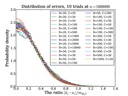
  (a) Distribution of $E_{p}/m_{R,C}$ for various $R,C$. Note that it is nearly independent of $R$ and $C$.

  

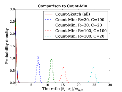
  (b) Same as (a), but with Count-Min added for comparison. Note that Count-Min has larger error than Count-Sketch.

  Figure 1: Histograms of the point error $E_{p}$

• (Theorem 7.1) After removing $n2^{-\Omega(R)}$ probability mass, the top-$k$ estimation error has expectation

  $$\operatorname*{\mathbb{E}}[E_{k}]\simeq\sqrt{k}m_{R,C}.$$

  Furthermore, as $k$ increases, $E_{k}$ concentrates more strongly about its mean:

  $$\Pr[E_{k}>2\operatorname*{\mathbb{E}}[E_{k}]]\lesssim 1/k.$$

Our results are presented in the form of a series of figures.

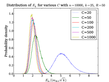
(a) Distribution of $E_{k}/(m_{R,C}\sqrt{k})$ for multiple $C$. Once $C$ is large enough, the distribution is fairly static.

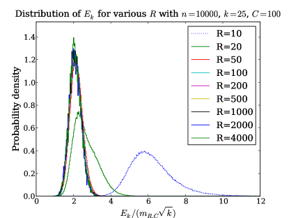
(b) Distribution of $E_{k}/(m_{R,C}\sqrt{k})$ for multiple $R$. Once $R$ is large enough, the distribution is fairly static.

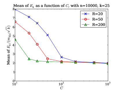
(c) $\operatorname*{\mathbb{E}}[E_{k}]/(m_{R,C}\sqrt{k})$ as a function of $C$. Above some threshold (depending on $R$), the mean remains fixed at a constant.

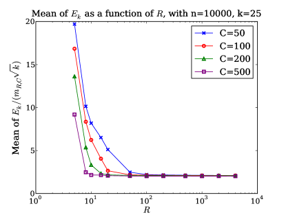
(d) $\operatorname*{\mathbb{E}}[E_{k}]/(m_{R,C}\sqrt{k})$ as a function of $R$. Above some threshold (depending on $C$), the mean remains fixed at a constant.

Figure 2: Experimental results for the top-$k$ error $E_{k}$

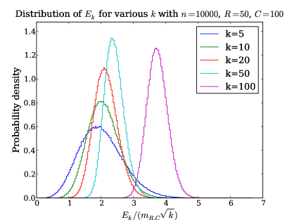
(a) Distribution of $E_{k}/(m_{R,C}\sqrt{k})$ for varying $k$. For small $k$, as $k$ increases the distribution becomes narrower and remains roughly in place. For larger $k$, as $k$ increases the distribution instead shifts to the right.

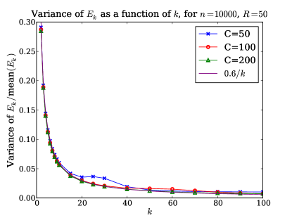
(b) The variance of $E_{k}/\operatorname*{\mathbb{E}}[E_{k}]$, as a distribution over $k$. It appears to be approximated well by $0.6/k$.

Figure 3: Experimental results for the variation of the top-$k$ error $E_{k}$

Figure 1LABEL:sub@f:ped shows the probability density function of $E_{p}/m_{R,C}$ for $n=10^{6}$ and many different pairs $(R,C)$. We find that the PDFs all look fairly similar, and match a Gaussian with constant standard deviation. For comparison, Figure 1LABEL:sub@f:pecm shows the equivalent error when using the Count-Min sketch of Cormode and Muthukrishnan [CM04]. We find that Count-Min gives asymptotically higher error for the estimation of each coordinate.

We study the distribution of $E_{k}$ in Figure 2. Figures 2(a) and 2(b) give the probability density functions of $E_{k}/(m_{R,C}\sqrt{k})$ for various $R$ and $C$, respectively. In both cases, we find that once $R$ and $C$ reach a threshold, the distribution remains roughly constant—and has a constant mean—as $R$ and $C$ increase beyond that point. Figures 2(c) and 2(d) show how $\operatorname*{\mathbb{E}}[E_{k}]$ changes as a function of $R$ and $C$, respectively. As predicted, we find that $E_{k}/(m_{R,C}\sqrt{k})$ has constant mean—so $E_{k}$ scales as $m_{R,C}\sqrt{k}$—after $R$ and $C$ are sufficiently large. The threshold above which $E_{k}/(m_{R,C}\sqrt{k})\approx 3$ allows some trade-off between $R$ and $C$. At $n=10^{4}$ and $k=25$, we observe that $(R,C)=(26,100)\approx(2\log_{2}n,4k)$ is above the threshold.

In Figure 3, we consider how well $E_{k}$ concentrates about its mean as a function of $k$. In 3(a), we plot the PDF of $E_{k}/(m_{R,C}\sqrt{k})$ for various values of $k$. We observe that as $k$ increases, the distribution becomes more tightly distributed about its mean. However, once $k$ is large enough, our chosen $(R,C)$ is no longer above the threshold for $(n,k)$, causing the distribution of $E_{k}/(m_{R,C}\sqrt{k})$ to shift markedly to the right and stop becoming more tightly distributed. In 3(b), we plot the variance of $E_{k}/\operatorname*{\mathbb{E}}[E_{k}]$, as a function of $k$. We find that it is $\Theta(1/k)$, which gives

$$\Pr[E_{k}>2\operatorname*{\mathbb{E}}[E_{k}]]\lesssim 1/k.$$

This is the analog of Theorem 6.5.

Appendix A Proofs for Concentration of Sets

In this section our aim is to prove Proposition 5.1. Our approach is to study the pairwise correlations between errors in coordinates. We do this in two parts. We first define a variant of Count-Sketch, which we call tail-independent modified (TIM) Count-Sketch. In TIM Count-Sketch, the error coming from collisions with small elements (the “tail error”) is replaced by independent, uniform noise. We then focus on two fixed coordinates and define a further variant, fully-independent modified (FIM) Count-Sketch. In FIM Count-Sketch, the errors for our two coordinates of interest are fully independent. We define these variants in such a way that unmodified, TIM, and FIM Count-Sketch can all be sampled with the same randomness, so that they may be compared simultaneously. We then bound the covariance between coordinate errors in TIM Count-Sketch by bounding the difference between TIM and FIM, and use the resulting bound on the error of sets in TIM Count-Sketch to conclude a bound on unmodified Count-Sketch.

As in the statement of Proposition 5.1, let $S\subset[n]$ be a subset of indices with $\left|S\right|\leq k$; this is the set on which we will study concentration. In the first part of the argument we will work instead with $S^{\prime}:=S\cup[k]$, the set of interest together with the set of heavy hitters. Let $C=ck$ be the number of columns in our sketch, for sufficiently large constant $c$. Let $R\gtrsim\log k$ be the number of rows, and let $x$ be the vector we are sketching. Finally, define $\mu=\lVert x_{\overline{S^{\prime}}}\rVert_{2}/\sqrt{C}\leq\lVert x_{\overline{[k]}}\rVert_{2}/\sqrt{C}$.

Observation A.1.

Let $X$ be a symmetric random variable and suppose $\eta,\sigma>0$ are such that, for all $\epsilon\leq 1$, $\Pr[|X|<\epsilon\sigma]\geq\eta\epsilon$. (For instance, if $X$ is a random variable to which Corollary 3.2 applies and $\sigma^{2}=\operatorname*{\mathbb{E}}[X^{2}]$, then one can check that $\eta=1/7$ suffices.) Let $U$ be a symmetric random variable which is uniform on $[-1,1]$ with probability $\eta$ and otherwise is $\pm\infty$. Then $\Pr[|X|<\epsilon\sigma]\geq\Pr[\sigma|U|<\epsilon\sigma]$ for all $\epsilon$. It follows that we can sample $X$ and $U$ in such a way that they always have the same sign and satisfy $|X|\leq\sigma|U|$.

Lemma A.2.

As in a row of Count-Sketch, randomly assign to each $i\in\overline{S^{\prime}}$ a column $h(i)$ and a sign $s(i)$. For each column $j$ let $T_{j}=\sum_{i\in\overline{S^{\prime}}:h(i)=j}s(i)x_{i}$. Let $L$ be a subset of $\ell\leq 2k$ columns. There exist i.i.d. symmetric random variables $\{V_{j}:j\in L\}$ with the following properties: (i) $V_{j}$ is uniform on $[-\mu,\mu]$ with constant probability and otherwise is $\pm\infty$; (ii) $T_{j}$ and $V_{j}$ have the same sign; and (iii) $\left|T_{j}\right|\leq\left|V_{j}\right|$.

Proof.

Let $p=2\ell/C$, so that for each $i$ we have $\Pr[h(i)\in L]=\tfrac{1}{2}p$. Recalling that $C=ck$ for sufficiently large $c$, by taking $c\geq 8$ we can ensure $p\leq 1/2$.

Consider the following alternative procedure for sampling the random variables $\{T_{j}:j\in L\}$: for each $i\in\overline{S^{\prime}}$, decide with probability $p$ if $h(i)\in L$, and if so (1) assign $h(i)$ uniformly to one of the columns $j$ in $L$ and (2) add to $T_{j}$ a symmetric random variable which is $0$ with probability $1/2$ and otherwise is $\pm x_{i}$. (The variables $\{T_{j}:j\not\in L\}$ are not computed.) In other words, for each $i\in\overline{S^{\prime}}$ we double the probability of $h(i)\in L$, but offset that by introducing a $1/2$ probability that $i$ contributes zero. It is clear that this is equivalent to the original definition of $T_{j}$, so we henceforth work with it.

Now condition on the column assignments $h(i)$. Having done so, the variables $T_{j}$ are independent. Moreover, each is a sum of independent, symmetric random variables which are $0$ with probability $1/2$. Thus Corollary 3.2 applies. Let $\sigma_{j}$ be the standard deviation of $T_{j}$ and let $\{U_{j}:j\in L\}$ be a set of i.i.d. random variables distributed like the variable $U$ in Observation A.1. Then, by that observation, we can sample $T_{j}$ so that $T_{j}$ and $U_{j}$ have the same sign and $|T_{j}|\leq\sigma_{j}|U_{j}|$.

Removing the conditioning on column assignments, the dependence between columns manifests in the random variables $\sigma_{j}^{2}=\sum_{i\in\overline{S^{\prime}}:h(i)=j}x_{i}^{2}/2$ for $j\in L$. Consider the following procedure for sampling these variances.

1. Let $q\in(0,1)$ be the solution to the equation $(1-q)^{\ell}=1-p$.

2. For each $i\in\overline{S^{\prime}}$, determine preliminary column assignments by, for each column $j\in L$, deciding independently with probability $q$ if $i$ is to be placed in column $j$. These preliminary assignments may have repetitions and may not assign $i$ to any column.

3. If a coordinate $i$ is assigned to just one column, let that be $h(i)$. If it is assigned to more than one column, then randomly choose one of those columns to be $h(i)$. If it is assigned to no columns, then we set $h(i)\in\overline{L}$, i.e., we effectively just ignore $i$.

4. Let $\sigma_{j}^{2}=\sum_{i\in\overline{S^{\prime}}:h(i)=j}x_{i}^{2}/2$.

One can easily check that this is a valid way of sampling. The probability $q$ is the solution to the equation $\log(1-p)=\ell\log(1-q)$; since $\log(1-x)=\Theta(-x)$ for $\left|x\right|\leq 1/2$ it follows that $q=\Theta(p/\ell)=\Theta(1/C)$.

Let $\widehat{\sigma}_{j}^{2}$ be the variance that would have been obtained from this procedure had we omitted step 3, i.e., had we not corrected double-assignments. Note that the random variables $\{\widehat{\sigma}_{j}^{2}\}$ are i.i.d. and they satisfy $\sigma_{j}^{2}\leq\widehat{\sigma}_{j}^{2}$. In particular, we have $|T_{j}|\leq\widehat{\sigma}_{j}|U_{j}|$.

The random variables $\{\widehat{\sigma}_{j}^{2}:j\in L\}$ have expected value $\operatorname*{\mathbb{E}}[\widehat{\sigma}_{j}^{2}]=(q/2)\sum_{i\in\overline{S^{\prime}}}x_{i}^{2}=\Theta(\mu^{2})$. Thus, for any $\epsilon\leq 1$, by Markov’s inequality we have

$$\Pr[\widehat{\sigma}_{j}|U_{j}|\leq\epsilon\mu]\geq\Pr\left[\widehat{\sigma}^{2}_{j}<4\operatorname*{\mathbb{E}}[\widehat{\sigma}_{j}^{2}]\right]\cdot\Pr\left[|U_{j}|\leq\epsilon\cdot\frac{\mu}{2\sqrt{\operatorname*{\mathbb{E}}[\widehat{\sigma}_{j}^{2}]}}\right]\gtrsim\epsilon.$$

Applying Observation A.1 once more, we find symmetric random variables $V_{j}$ which are uniform on $[-\mu,\mu]$ with constant probability, which have the same sign as $U_{i}$ (and thus the same sign as $T_{j}$), and which always satisfy $|V_{j}|\geq\widehat{\sigma}_{j}|U_{j}|\geq|T_{j}|$. These random variables have all the desired properties.

Finally, we note that, as written, the random variables just constructed depend on $\ell$, in that $q$ depends on $\ell$. However, we can remove this dependence by simply choosing the largest $q$ over all $\ell\leq 2k$. This gives random variables which satisfy the same bounds but are agnostic about $\ell$. ∎

In a moment we will define the tail-independent modified (TIM) Count-Sketch. The main point of TIM Count-Sketch is to replace the actual contributions of the “tail” coordinates $\overline{[k]}$ with the independent, uniform random variables in Lemma A.2. There is one additional difference, though: for later use, we invent a notion of “ghost coordinates” for TIM Count-Sketch. We do this for the following reason. In TIM Count-Sketch, when there is a collision between two coordinates in $S^{\prime}$, we will assign them each a fixed error instead of using the tail noise. Later, when we modify TIM Count-Sketch to achieve full pairwise independence, it will be convenient to have a larger probability of using the fixed error than we get from just collisions between coordinates in $S^{\prime}$. The right probability for our uses lies somewhere between that which you get from considering collisions amongst $|S^{\prime}|$ coordinates and that which you get from considering collisions amongst $C+1$ coordinates. To achieve this intermediate probability, we fabricate $C+1-|S^{\prime}|$ “ghosts”. These are dummy coordinates whose only purpose is to (maybe) collide with coordinates of $S^{\prime}$ to force them to use the fixed error. To allow us to tune the probability of collision, each ghost may or may not be “real”, according to i.i.d. Bernoulli random variables. Thus the probability of a ghost colliding with a fixed coordinate $i$ is the probability of that ghost being real times the probability that it is assigned the same column as $i$.

We are now ready to give an actual definition. Fix a bound $M>0$ (later we will take $M=\mu$) and, for each row, compute estimates as follows.

1. Assign signs $s(i)$ and columns $h(i)$ to the elements of $S^{\prime}$.

2. Choose signs and columns for the elements of $\overline{S^{\prime}}$ and, for the columns $j$ occupied by elements of $S^{\prime}$, let $T_{j}$ and $V_{j}$ be as in Lemma A.2.

3. Fabricate $C+1-|S^{\prime}|$ ghost coordinates and, for each, decide independently with probability $p_{\text{ghost}}$ if that ghost is real. Random choose a column for each ghost that is real. (The probability $p_{\text{ghost}}$ will be chosen later.)

4. For each coordinate $i\in S^{\prime}$,

   1. Let $H_{i}$ be the sum of $s(i)s(j)x_{j}$ over all $j\in S^{\prime}$ with $j\neq i$ and $h(j)=h(i)$.

   2. Let $\sigma\in\{\pm 1\}$ be the sign of $H_{i}+s(i)T_{h(i)}$ (which would be the error in unmodified Count-Sketch).

   3. If $i$ is in the same column as $j$ for some $j\in S^{\prime}$, $j\neq i$ (i.e., if the sum defining $H_{i}$ is not empty) or if $i$ is in the same column as a ghost, then return $x_{i}+\sigma\cdot M$ as the estimate.

   4. Otherwise return $x_{i}+\sigma\cdot\min\{M,\left|V_{h(i)}\right|\}$ as the estimate for $i$ in this row.

The final estimate for each coordinate $i\in S^{\prime}$ is the median of the estimates in each row. (TIM Count-Sketch only yields estimates for the coordinates in $S^{\prime}$.)

The tail-independence modification can only worsen errors, in the following sense.

Observation A.3.

Suppose $a=\{a_{1},\dots,a_{n}\}$ and $b=\{b_{1},\dots,b_{n}\}$ are sequences such that, for each $i\in[n]$, $a_{i}$ and $b_{i}$ have the same sign and satisfy either $|a_{i}|\leq|b_{i}|$ or $|b_{i}|\geq M$. Then $\operatorname*{median}a_{i}$ and $\operatorname*{median}b_{i}$ have the same sign and satisfy either $\left|\operatorname*{median}a_{i}\right|\leq\left|\operatorname*{median}b_{i}\right|$ or $\left|\operatorname*{median}b_{i}\right|\geq M$.

Lemma A.4.

Let $\widehat{x}_{\text{tim}}$ be the estimate of $x$ using TIM Count-Sketch and let $\widehat{x}_{\text{um}}$ be the estimate using unmodified Count-Sketch. For any subset $A\subset(-M,M)^{|S|}$ which is convex and symmetric in each coordinate,

$$\Pr[(\widehat{x}_{\text{um}}-x)_{S}\in A]\geq\Pr[(\widehat{x}_{\text{tim}}-x)_{S}\in A].$$

Proof.

Note that unmodified Count-Sketch can be run simultaneously with TIM Count-Sketch, using the same randomness. Consider a fixed row and a fixed coordinate $i\in S$. Keeping the notation above, the error $E_{\text{tim}}$ arising from TIM Count-Sketch is $\sigma\cdot M$ if there is a collision or $\sigma\cdot\min\{M,|V_{h(i)}|\}$ if not. The error $E_{\text{um}}$ arising from unmodified Count-Sketch is $H_{i}+s(i)T_{h(i)}$. Clearly $E_{\text{tim}}$ and $E_{\text{um}}$ always have the same sign and satisfy either $\left|E_{\text{um}}\right|\leq\left|E_{\text{tim}}\right|$ or $\left|E_{\text{tim}}\right|\geq M$. The final errors in the estimates are medians of these row errors. Thus, by Observation A.3,

$$\left|(\widehat{x}_{\text{um}}-x)_{i}\right|\leq\left|(\widehat{x}_{\text{tim}}-x)_{i}\right|$$

or else the TIM error is at least $M$. In other words, given this method of sampling, whenever the error for TIM Count-Sketch is less than $M$ we know that the error for unmodified Count-Sketch is no bigger than the error for TIM Count-Sketch. This clearly proves what we wanted. ∎

Now that we have arranged for independence of the tail contributions, the only remaining dependence arises from collisions amongst the elements of $S^{\prime}$. Fix two coordinates $i_{1},i_{2}\in S^{\prime}$; we will bound the correlation between the errors in these two coordinates. Analogously to our analysis of $\sigma_{j}$ in Lemma A.2, we can highlight the dependence by first pretending collisions are independent and then correcting double-collisions. More precisely, consider the following alternative mechanism for determining collisions.

1. Let $\mathfrak{p}\colon[0,\tfrac{1}{2}]\rightarrow[0,1]$ denote the inverse of the monotone-increasing function $p\mapsto p/(1+p)$.

2. For starters, declare that $i_{1}$ and $i_{2}$ do not collide. (This may change later in the procedure.)

3. For each element $j$ of $S^{\prime}\setminus\{i_{1},i_{2}\}$ (resp., each ghost) and each of $i=i_{1},i_{2}$, independently decide with probability $\mathfrak{p}(1/C)$ (resp., $\mathfrak{p}(p_{\text{ghost}}/C)$) if $j$ collides with $i$. Note that, because these decisions are independent, there may well be double-collisions at this stage.

4. If any ghost or coordinate in $S^{\prime}$ collides with both $i_{1}$ and $i_{2}$, then resample everything according to the correct distribution, conditioned on $i_{1}$ and $i_{2}$ colliding.

Using this procedure, the event that $i_{1}$ and $i_{2}$ end up not colliding is the same as the event that step 3 produced no double-collisions. The probability of this is

$$p_{\text{nc}}(p_{\text{ghost}}):=\Pr[\text{$i_{1},i_{2}$ do not collide}]=(1-\mathfrak{p}(1/C)^{2})^{|S^{\prime}|-2}(1-\mathfrak{p}(p_{\text{ghost}}/C)^{2})^{C+1-|S^{\prime}|}.$$

This is a monotone-decreasing function of $p_{\text{ghost}}$. Noting that $\mathfrak{p}(1/C)=1/(C-1)$, we see that

$$p_{\text{nc}}(0)=\left(1-\frac{1}{(C-1)^{2}}\right)^{|S^{\prime}|-2}\geq\left(1-\frac{1}{(C-1)^{2}}\right)^{2k}=1-\frac{1}{C}\cdot\Theta\left(\frac{k}{C}\right)$$

and

$$p_{\text{nc}}(1)=\left(1-\frac{1}{(C-1)^{2}}\right)^{C-1}.$$

By taking $C$ to be a suitably large multiple of $k$ we can arrange for $p_{\text{nc}}(0)$ to be at least $1-1/C$. By a simple calculus exercise, $p_{\text{nc}}(1)\leq 1-1/C$. Thus there is a unique $q\in[0,1]$ such that $p_{\text{nc}}(q)=1-1/C$. We now and henceforth set $p_{\text{ghost}}$ to this value of $q$.

This is supposed to be an alternative, but equivalent, method for determining collisions. Before continuing, let us check that it is indeed equivalent. Our choice of $p_{\text{ghost}}$ guaranteed that the new mechanism has the right probability of $i_{1}$ and $i_{2}$ colliding; moreover, when they do collide, we explicitly sample according to the correct distribution. Thus, to demonstrate equivalence, we need only to consider the case when $i_{1}$ and $i_{2}$ do not collide. Condition on this event and consider the (conditional) probability of some other coordinate $j\in S^{\prime}\setminus\{i_{1},i_{2}\}$ colliding with $i_{1}$. Using the original sampling mechanism, this probability is $1/C$. Using our alternative sampling mechanism, the probability is

$$\Pr[\text{$j$ collides with $i_{1}$}\mid\text{$i_{1},i_{2}$ do not collide}]$$

$$= \Pr[\text{$j$ collides with $i_{1}$ in step $3$}\mid\text{there are no double-collisions in step 3}].$$

The event that there is no double-collision is the intersection of independent events for each element of $S^{\prime}\setminus\{i_{1},i_{2}\}$ and for each ghost. Of these constituent events, only one is relevant to the conditional probability we want to compute: the event that $j$ does not double-collide. Thus our probability is

$$\Pr[\text{$j$ collides with $i_{1}$ in step $3$}\mid\text{$j$ does not collide with both $i_{1}$ and $i_{2}$ in step 3}]$$

$$= \frac{\mathfrak{p}(1/C)-\mathfrak{p}(1/C)^{2}}{1-\mathfrak{p}(1/C)^{2}}=\frac{\mathfrak{p}(1/C)}{1+\mathfrak{p}(1/C)}=\frac{1}{C},$$

which is what we wanted. One can similarly check that the probability of a ghost collision is correct. Thus, as claimed, our new scheme is a valid way to sample the collision events.

We can now define our last variant of Count-Sketch, fully-independent modified (FIM) Count-Sketch. This only produces estimates for the two coordinates $i_{1}$ and $i_{2}$. For each row, the FIM estimate is computed as follows. We always specify that $i_{1}$ and $i_{2}$ will not collide. To determine which elements of $S^{\prime}\setminus\{i_{1},i_{2}\}$ and which ghosts collide with $i_{1}$ and $i_{2}$, we use (1–3) of the “alternative mechanism” above. We omit step 4, so that a given coordinate may collide with both $i_{1}$ and $i_{2}$. Then, for each $i\in\{i_{1},i_{2}\}$ and for each coordinate colliding with $i$, we choose a random sign. (In particular, if some coordinate is supposed to collide with both $i_{1}$ and $i_{2}$, then it is associated with two different, independent random signs.) Using these collision and sign data, we proceed as in (4a–4d) of the description of TIM Count-Sketch to get a row estimate. As always, the final estimate is the median of the row estimates.

In each row, the estimates for $i_{1}$ and $i_{2}$ produced by FIM Count-Sketch are independent; thus the final estimates are also independent.

FIM and, to a lesser extent, TIM Count-Sketch are quite a bit different from unmodified Count-Sketch. However, for a single coordinate they preserve many of the salient features. In particular, all of the properties used in the proof of Theorem 4.1 still hold: rows are independent, the errors in each row are symmetric, and in each row we have (i) with constant probability, there is no collision with $[k]$ and (ii) the error arising from collisions with $\overline{[k]}$ satisfies the bound of Corollary 3.2. Thus, with the same proof as Theorem 4.1, we have the following bounds.

Lemma A.5.

Fix $i\in\{i_{1},i_{2}\}$ and consider the estimates $(\widehat{x}_{\text{tim}})_{i}$ and $(\widehat{x}_{\text{fim}})_{i}$ of $x_{i}$ from TIM and FIM Count-Sketch, respectively. For any $t\leq R$ we have

$$\Pr\left[((\widehat{x}_{\text{tim}})_{i}-x_{i})^{2}>\frac{t}{R}\cdot\frac{\lVert x_{\overline{[k]}}\rVert_{2}^{2}}{k}\right]<2e^{-\Omega(t)}\quad\text{and}\quad\Pr\left[((\widehat{x}_{\text{fim}})_{i}-x_{i})^{2}>\frac{t}{R}\cdot\frac{\lVert x_{\overline{[k]}}\rVert_{2}^{2}}{k}\right]<2e^{-\Omega(t)}.$$

Corollary A.6.

Suppose $M=\Theta(\mu)$. Then

$\begin{array}[]{lclc}\operatorname*{\mathbb{E}}[((\widehat{x}_{\text{tim}})_{i}-x_{i})^{2}]\lesssim\dfrac{\mu^{2}}{R}&,&\operatorname*{\mathbb{E}}[((\widehat{x}_{\text{tim}})_{i}-x_{i})^{4}]\lesssim\dfrac{\mu^{4}}{R^{2}}&,\\ \operatorname*{\mathbb{E}}[((\widehat{x}_{\text{fim}})_{i}-x_{i})^{2}]\lesssim\dfrac{\mu^{2}}{R}&\text{, and}&\operatorname*{\mathbb{E}}[((\widehat{x}_{\text{fim}})_{i}-x_{i})^{4}]\lesssim\dfrac{\mu^{4}}{R^{2}}&.\end{array}$

We can recover TIM Count-Sketch from FIM Count-Sketch by resampling some of the rows. More specifically, we take any row in which some ghost or some element of $S^{\prime}$ collides with both $i_{1}$ and $i_{2}$ and resample that row, conditioning on $i_{1}$ and $i_{2}$ colliding with each other. The errors for both $i_{1}$ and $i_{2}$ in any such row are $M$ in magnitude both before and after resampling. Moreover, for a fixed coordinate $i\in\{i_{1},i_{2}\}$ the signs of the errors before and after resampling are independent and uniform. (Note: the signs of the errors for $i_{1}$ and $i_{2}$ after resampling are not necessarily independent of each other. We assume nothing about their dependence in our argument.)

Let $\widehat{x}_{\text{fim}}$ be the estimate computed by FIM Count-Sketch and let $\widehat{x}_{\text{tim}}$ be the result of TIM Count-Sketch, recovered from FIM Count-Sketch as above. Let $\widetilde{R}$ be the number of rows that have to be resampled to recover TIM Count-Sketch from FIM Count-Sketch. Focusing for the moment on $i_{1}$, define the errors

$$E_{\text{fim}}=(\widehat{x}_{\text{fim}}-x)_{i_{1}}\ \ \ \text{and}\ \ \ E_{\text{tim}}=(\widehat{x}_{\text{tim}}-x)_{i_{1}}.$$

We expect $\widetilde{R}$ to be reasonably small, and thus we expect the change in moving from FIM to TIM to be small. In particular, we expect $E_{\text{fim}}$ and $E_{\text{tim}}$ to be close. More specifically, we shall prove the following proposition.

Proposition A.7.

Suppose $M=\Theta(\mu)$. Then $\displaystyle\operatorname*{\mathbb{E}}[(E_{\text{tim}}^{2}-E_{\text{fim}}^{2})^{2}]\lesssim\frac{M^{4}}{R^{2}k^{1/7}}$.

Since we just want to bound the expected value of a bounded random variable, small probability events can be ignored. Indeed, in general, if $X$ is a random variable bounded by $B$ and $\mathcal{E}$ is an event with probability $p$, then

$$\operatorname*{\mathbb{E}}[X]=p\operatorname*{\mathbb{E}}[X\mid\mathcal{E}]+(1-p)\operatorname*{\mathbb{E}}[X\mid\overline{\mathcal{E}}]\leq pB+\operatorname*{\mathbb{E}}[X\mid\overline{\mathcal{E}}].$$

Thus if we aim to prove $\operatorname*{\mathbb{E}}[X]\lesssim Y$ and we know $pB\lesssim Y$, then it suffices to prove $\operatorname*{\mathbb{E}}[X\mid\overline{\mathcal{E}}]\lesssim Y$. Specializing to our case, because $\left|E_{\text{fim}}\right|,\left|E_{\text{tim}}\right|\leq M$ always holds, this demonstrates that in order to prove Proposition A.7, we may condition away from events that occur with probability $O(R^{-2}k^{-1/7})$. We will refer to such events as “ignorable” and, as the name indicates, freely ignore them.

Lemma A.8.

If $k\geq R^{7/2}$ then Proposition A.7 holds.

Proof.

The probability that a single row is not resampled is $p_{\text{nc}}=1-1/C$, and so

$$\Pr[\widetilde{R}=0]=\left(1-\frac{1}{C}\right)^{R}=\exp(R\log(1-1/C))=\exp(-R\Theta(1/C))=1-\Theta\left(\frac{R}{C}\right).$$

Because $C=\Omega(k)$ and $k\geq R^{7/2}$, $R/C\lesssim R/k\lesssim R^{-2}k^{-1/7}$. Thus $\widetilde{R}>0$ is an ignorable event. But of course if $\widetilde{R}=0$ then $\widehat{x}_{\text{fim}}=\widehat{x}_{\text{tim}}$. This gives the desired bound. ∎

Observation A.9.

Let $a,b,c>0$ be arbitrary. Any event that occurs with probability $\exp(-\Omega(R^{b}k^{c}))$ is ignorable. Moreover, if we suppose that $k\leq R^{a}$, then any event that occurs with probability $\exp(-\Omega(R^{b}))$ is ignorable.

Lemma A.10.

Suppose $k\leq R^{7/2}$. Then, except for ignorable events, $\widetilde{R}<R/k^{1/5}$.

Proof.

Each row is resampled with probability $1/C$, and the resampling events for the $R$ rows are independent. Thus, by the Chernoff bound $\Pr[X\geq(1+\epsilon)\operatorname*{\mathbb{E}}[X]]\leq\exp(-\operatorname*{\mathbb{E}}[X]\epsilon^{2}/(2+\epsilon))$ (applied with $\epsilon=C/k^{1/5}$, which in particular can be taken to be arbitrarily large),

$$\Pr\left[\widetilde{R}\geq\frac{R}{k^{1/5}}\right]\leq\exp(-\Omega(R/k^{1/5}))=\exp(-\Omega(R^{3/10})).$$

This is ignorable by Observation A.9. ∎

Let $\widetilde{R}_{+},\widetilde{R}_{0},\widetilde{R}_{-}$ be the number of rows resampled in which the error increases from $-M$ to $M$, stays the same, and decreases with $M$ to $-M$, respectively. Thus $\widetilde{R}_{+}+\widetilde{R}_{0}+\widetilde{R}_{-}=\widetilde{R}$. The net effect of resampling is measured by $\widehat{R}:=\widetilde{R}_{+}-\widetilde{R}_{-}$.

Lemma A.11.

Fix a positive integer $r$. If $X$ is an $(N,p)$ binomial random variable with $Np\geq 1$, then $\operatorname*{\mathbb{E}}[(X-Np)^{r}]\lesssim(Np)^{r/2}$ (where the implied constant depends on $r$).

Proof.

Let $Y$ be a random variable with $\Pr[Y=1-p]=p$ and $\Pr[Y=-p]=1-p$, and let $X-Np=Y_{1}+\cdots+Y_{N}$ where $Y_{1},\dots,Y_{N}$ are i.i.d. with the same distribution as $Y$. Then

$$\operatorname*{\mathbb{E}}[(X-Np)^{r}]=\operatorname*{\mathbb{E}}[(Y_{1}+\cdots+Y_{N})^{r}]=\sum_{m=1}^{\min\{r,N\}}\sum_{\begin{subarray}{c}e_{1}\geq\cdots\geq e_{m}\geq 1\\ \sum e_{i}=r\end{subarray}}C_{e_{1},\dots,e_{m}}\operatorname*{\mathbb{E}}[Y^{e_{1}}]\cdots\operatorname*{\mathbb{E}}[Y^{e_{m}}],$$

where the coefficient $C_{e_{1},\dots,e_{m}}$ counts the number of ways to choose an $r$-tuple of elements of an $N$-element set such that the most common element occurs $e_{1}$ times, the next most common element occurs $e_{2}$ times, and so on.

We have $\operatorname*{\mathbb{E}}[Y]=0$, so the terms with $e_{i}=1$ (for any $i$) all vanish. Since $\sum_{i=1}^{m}e_{i}=r$, this leaves just the terms with $m\leq r/2$. Now for any $e\geq 2$, we have

$$\operatorname*{\mathbb{E}}[Y^{e}]=p(1-p)^{e}+(1-p)(-p)^{e}\leq p(1-p)^{2}+(1-p)p^{2}=p(1-p)\leq p,$$

and so

$$\operatorname*{\mathbb{E}}[(X-Np)^{r}]\leq\sum_{m=1}^{\min\{r/2,N\}}\sum_{\begin{subarray}{c}e_{1}\geq\cdots\geq e_{m}\geq 2\\ \sum e_{i}=r\end{subarray}}C_{e_{1},\dots,e_{m}}p^{m}.$$

Now we can compute $C_{e_{1},\dots,e_{m}}$ by first choosing which $m$ of the $N$ elements occur and then choosing how to arrange them. The number of choices for the former is clearly bounded by $N^{m}$ and the number of choices for the latter is bounded by a function of $r$ only. Thus $C_{e_{1},\dots,e_{m}}\lesssim N^{m}$. Moreover, the number of terms in the second summation is bounded by a function of $r$ only. This leaves us with

$$\operatorname*{\mathbb{E}}[(X-Np)^{r}]\lesssim\sum_{m=1}^{\min\{r/2,N\}}N^{m}p^{m}.$$

Given that $Np\geq 1$, the last term in the summation is dominant, giving the desired bound. ∎

Lemma A.12.

Suppose $k\leq R^{7/2}$. Conditioning away from ignorable events, $\operatorname*{\mathbb{E}}[\widehat{R}^{4}]\lesssim R^{2}/k^{2/5}$.

Proof.

By reducing $\widetilde{R}$, we may assume without loss of generality that $\widehat{R}_{0}=0$. Thus $\widehat{R}$ is just the value of a discrete random walk of length $\widetilde{R}$. By Lemma A.11 the fourth moment of such a random walk is $O(\widetilde{R}^{2})$. Combining this with Lemma A.10 gives the desired bound. ∎

Lemma A.13.

Suppose $k\leq R^{7/2}$ and $M=\Theta(\mu)$. Conditioning away from ignorable events and then conditioning on the value of $\widehat{R}$, $\operatorname*{\mathbb{E}}[(E_{\text{tim}}-E_{\text{fim}})^{4}]\lesssim(M\widehat{R}/R)^{4}$.

• First, suppose $\widehat{R}=0$. In this case $E_{\text{fim}}=E_{\text{tim}}$, so the desired bound holds because both sides are $0$. Thus we may suppose $\widehat{R}\neq 0$; moreover, by symmetry we may assume $\widehat{R}>0$. In this case we have $E_{\text{tim}}\in[E_{\text{fim}},M]$.

  By Lemma A.5 we see that $\Pr[|E_{\text{fim}}|>M/2]<e^{-\Omega(R)}$; thus, by Observation A.9, the corresponding event is ignorable. For the remainder of the proof, assume that it does not happen.

  Condition for a moment on both the value of $E_{\text{fim}}$ and on the set of $R/2$ rows in which the error for FIM Count-Sketch is above the median. Pick one such row $r$ and consider its error $E_{r}$. Before the conditioning, using the assumption $M=\Theta(\mu)$, the distribution for $E_{r}$ consisted of atoms at $\pm M$ and $\Omega(1)$ probability of being uniform in $[-M,M]$. The net effect of our conditioning is to simply condition on $E_{r}\geq E_{\text{fim}}$. (By conditioning first on $r$ having above-median error, we removed the nontrivial dependence between $E_{\text{fim}}$ and $E_{r}$.) In particular, with $\Omega(1)$ probability, $E_{r}\in[E_{\text{fim}},M)$. (And, when this occurs, $E_{r}$ is uniform in that interval.) Applying a Chernoff bound to the $R/2$ such rows, we see that, with probability $1-e^{-\Omega(R)}$, there are $\Omega(R)$ rows in which the error lies in $[E_{\text{fim}},M)$. Since the failure probability is ignorable, we henceforth assume that this holds.

  (Note that the ignorable events we just conditioned away influence $\widehat{R}$. We conditioned on them first to remove that dependence.)

  Fix $t>0$ and consider the event $\mathcal{E}_{t}:=\{E_{\text{tim}}>E_{\text{fim}}+tM\widehat{R}/R\}$. Since the difference between TIM and FIM Count-Sketch is just replacing $\widehat{R}$ rows with error $-M$ by rows with error $+M$, this event is equivalent to FIM Count-Sketch having fewer than $\widehat{R}$ rows in which the error is in the interval $I=[E_{\text{fim}},E_{\text{fim}}+tM\widehat{R}/R]$. Given the above discussion, there are $\Omega(R)$ rows in which the probability of the error lying in that interval is $\Omega(t\widehat{R}/R)$. More explicitly, for some constants $a$ and $b$, there are $N:=aR$ rows in which the probability of the error lying in $I$ is (at least) $p:=bt\widehat{R}/R$. Let $X$ be the total number of such rows. Then $X$ is a $(N,p)$ binomial random variable. For $t>t_{0}:=1/(ab)$ (i.e., for all $t$ larger than a sufficiently large constant), we have $abt>1$. In particular this implies $Np>\widehat{R}\geq 1$, whence the $10$th moment of $X$ is $O((Np)^{5})$ by Lemma A.11. It also implies that $\widehat{R}<\operatorname*{\mathbb{E}}[X]=abt\widehat{R}$. Thus, by Markov’s inequality, à la Chebyshev’s inequality,

  $$\Pr[\mathcal{E}_{t}]=\Pr[X<\widehat{R}]\leq\frac{\operatorname*{\mathbb{E}}[(X-abt\widehat{R})^{10}]}{\widehat{R}^{10}(abt-1)^{10}}\lesssim\frac{(abt\widehat{R})^{5}}{\widehat{R}^{10}(abt-1)^{10}}\leq\frac{(abt)^{5}}{(abt-1)^{10}}.$$

  For, say, $t\geq 2t_{0}$, this is asymptotically $\lesssim t^{-5}$.

  Using integration by parts,

  $$\operatorname*{\mathbb{E}}[(E_{\text{tim}}-E_{\text{fim}})^{4}]=\left(\frac{M\widehat{R}}{R}\right)^{4}\cdot\int_{0}^{\infty}4t^{3}\cdot\Pr[\mathcal{E}_{t}]\ \text{d}t.$$

  Writing

  $$\int_{0}^{\infty}4t^{3}\cdot\Pr[\mathcal{E}_{t}]\ \text{d}t=\int_{0}^{2t_{0}}4t^{3}\cdot\Pr[\mathcal{E}_{t}]\ \text{d}t+\int_{2t_{0}}^{\infty}4t^{3}\cdot\Pr[\mathcal{E}_{t}]\ \text{d}t,$$

  the first term is $O(1)$ because $t_{0}$ is a constant. The second is $\lesssim\int_{2t_{0}}^{\infty}t^{-2}\ \text{d}t$, which is also $O(1)$. Thus, as desired,

  $$\operatorname*{\mathbb{E}}[(E_{\text{tim}}-E_{\text{fim}})^{4}]\lesssim\left(\frac{M\widehat{R}}{R}\right)^{4}.$$

We are now ready to complete the

Proof of Proposition A.7.

After Lemma A.8 it only remains to handle the case $k\leq R^{7/2}$. Combining Lemmas A.12 and A.13, we have $\operatorname*{\mathbb{E}}[(E_{\text{tim}}-E_{\text{fim}})^{4}]\lesssim M^{4}/(R^{2}k^{2/5})$. Applying Lemma A.5 and the union bound, we see that $\operatorname*{\mathbb{E}}[(E_{\text{tim}}+E_{\text{fim}})^{4}]\lesssim M^{4}/R^{2}$. Thus,

$$\operatorname*{\mathbb{E}}[(E_{\text{tim}}^{2}-E_{\text{fim}}^{2})^{2}] =\operatorname*{\mathbb{E}}[(E_{\text{tim}}-E_{\text{fim}})^{2}(E_{\text{tim}}+E_{\text{fim}})^{2}]$$

$$\leq\sqrt{\operatorname*{\mathbb{E}}[(E_{\text{tim}}-E_{\text{fim}})^{4}]\operatorname*{\mathbb{E}}[(E_{\text{tim}}+E_{\text{fim}})^{4}]}$$

$$\lesssim\frac{M^{4}}{R^{2}k^{1/5}},$$

which gives the desired bound a fortiori. ∎

Using these lemmata, we can finally prove the desired result.

Proposition 5.1.

Fix a constant $t>0$ and consider the estimate $\widehat{x}$ of $x$ from Count-Sketch using $R$ rows and $C=ck$ columns, $\log k\lesssim R$, for sufficiently large (depending on $t$) constant $c$. For any set $S\subset[n]$ with $\left|S\right|\leq k$,

$$\Pr\left[\lVert\widehat{x}_{S}-x_{S}\rVert_{2}^{2}>t\cdot\left|S\right|\cdot\frac{1}{R}\cdot\frac{\lVert x_{\overline{[k]}}\rVert_{2}^{2}}{k}\right]\lesssim\frac{1}{\left|S\right|^{1/14}}.$$

Proof.

Throughout we condition on the error for each coordinate in $S$ being less than $\mu$. By Theorem 4.1 and a union bound, this occurs with probability $1-|S|e^{-\Omega(R)}=1-k^{-\Omega(1)}$, so this conditioning can be absorbed into the final bound.

In addition to unmodified Count-Sketch, consider running TIM Count-Sketch with $M=\mu$. Define the convex, coordinate-wise symmetric set

$$A=\left\{v\in(-\mu,\mu)^{|S|}:\lVert v\rVert_{2}^{2}\leq t\cdot\left|S\right|\cdot\frac{1}{R}\cdot\frac{\lVert x_{\overline{[k]}}\rVert_{2}^{2}}{k}\right\}.$$

Applying Lemma A.4 with this set $A$ shows that unmodified Count-Sketch has at least as high of a probability of its error lying in $A$ as TIM Count-Sketch. Thus it suffices to prove the asserted probability bound for the TIM estimate $\widehat{x}_{\text{tim}}$.

The error we are studying is $\lVert(\widehat{x}_{\text{tim}}-x)_{S}\rVert_{2}^{2}=\sum_{i\in S}E_{\text{tim},i}^{2}$, where $E_{\text{tim},i}:=(\widehat{x}_{\text{tim}}-x)_{i}$. By Corollary A.6, $\operatorname*{\mathbb{E}}[E_{\text{tim},i}^{2}]\leq a\mu^{2}/R$ for some constant $a>0$. Now, by Chebyshev’s inequality, we have

$$\Pr\left[\lVert(\widehat{x}_{\text{tim}}-x)_{S}\rVert_{2}^{2}>(a+1)\cdot\frac{|S|\mu^{2}}{R}\right] \leq\Pr\left[\lVert(\widehat{x}_{\text{tim}}-x)_{S}\rVert_{2}^{2}-\operatorname*{\mathbb{E}}[\lVert(\widehat{x}_{\text{tim}}-x)_{S}\rVert_{2}^{2}]>\frac{|S|\mu^{2}}{R}\right]$$

$$\leq\frac{\operatorname*{Var}(\lVert(\widehat{x}_{\text{tim}}-x)_{S}\rVert_{2}^{2})}{(|S|\mu^{2}/R)^{2}}.$$ (7)

Thus we need to bound

$$\operatorname*{Var}(\lVert(\widehat{x}_{\text{tim}}-x)_{S}\rVert_{2}^{2})=\sum_{i\in S}\operatorname*{Var}(E_{\text{tim},i}^{2})+\sum_{i_{1}\neq i_{2}\in S}\operatorname*{Cov}(E_{\text{tim},i_{1}}^{2},E_{\text{tim},i_{2}}^{2}).$$ (8)

For each $i$ we have $\operatorname*{Var}(E_{\text{tim},i}^{2})\leq\operatorname*{\mathbb{E}}[E_{\text{tim},i}^{4}]\lesssim\mu^{4}/R^{2}$ by Corollary A.6. The covariance term is the harder part to control. Fix two coordinates $i_{1}\neq i_{2}\in S$ and consider FIM Count-Sketch with respect to those two coordinates. For shorthand write $E_{\text{tim},j}$ for $E_{\text{tim},i_{j}}$ ($j=1,2$) and define $E_{\text{fim},j}=(\widehat{x}_{\text{fim}}-x)_{i_{j}}$. Then

$$\begin{split}\operatorname*{Cov}(E_{\text{tim},1}^{2},E_{\text{tim},2}^{2})=&\operatorname*{Cov}(E_{\text{fim},1}^{2},E_{\text{fim},2}^{2})\\ &\quad+\operatorname*{Cov}(E_{\text{fim},1}^{2},E_{\text{tim},2}^{2}-E_{\text{fim},2}^{2})+\operatorname*{Cov}(E_{\text{fim},2}^{2},E_{\text{tim},1}^{2}-E_{\text{fim},1}^{2})\\ &\quad+\operatorname*{Cov}(E_{\text{tim},1}^{2}-E_{\text{fim},1}^{2},E_{\text{tim},2}^{2}-E_{\text{fim},2}^{2}).\end{split}$$

The first term vanishes because, by construction, $(\widehat{x}_{\text{fim}})_{i_{1}}$ and $(\widehat{x}_{\text{fim}})_{i_{2}}$ are independent. We shall bound the remaining terms using the Cauchy-Schwarz inequality $\operatorname*{Cov}(X,Y)\leq\sqrt{\operatorname*{Var}(X)\operatorname*{Var}(Y)}$.

By Corollary A.6 we have $\operatorname*{Var}(E_{\text{fim},j}^{2})\leq\operatorname*{\mathbb{E}}[E_{\text{fim},j}^{4}]\lesssim\mu^{4}/R^{2}$. By Proposition A.7, $\operatorname*{Var}(E_{\text{tim},j}^{2}-E_{\text{fim},j}^{2})\lesssim\mu^{4}/(R^{2}k^{1/7})$. Thus

$$\operatorname*{Cov}(E_{\text{tim},1}^{2},E_{\text{tim},2}^{2})\lesssim 2\cdot\frac{\mu^{4}}{R^{2}k^{1/14}}+\frac{\mu^{4}}{R^{2}k^{1/7}}\lesssim\frac{\mu^{4}}{R^{2}k^{1/14}}.$$

Substituting back into (8),

$$\operatorname*{Var}(\lVert(\widehat{x}_{\text{tim}}-x)_{S}\rVert_{2}^{2})\lesssim|S|\cdot\frac{\mu^{4}}{R^{2}}+|S|(|S|-1)\cdot\frac{\mu^{4}}{R^{2}k^{1/14}}\lesssim|S|^{2-\tfrac{1}{14}}\cdot\frac{\mu^{4}}{R^{2}}.$$

And finally, substituting this into (7), we get the desired bound. ∎

References

- [BCDH10] R. G. Baraniuk, V. Cevher, M. F. Duarte, and C. Hegde. Model-based compressive sensing. IEEE Transactions on Information Theory, 56, No. 4:1982–2001, 2010.
- [BKM+00] A. Broder, R. Kumar, F. Maghoul, P. Raghavan, S. Rajagopalan, R. Stata, A. Tomkins, and J. Wiener. Graph structure in the web. Comput. Netw., 33(1-6):309–320, 2000.
- [CCF02] M. Charikar, K. Chen, and M. Farach-Colton. Finding frequent items in data streams. ICALP, 2002.
- [CH10] G. Cormode and M. Hadjieleftheriou. Methods for finding frequent items in data streams. The VLDB Journal, 19(1):3–20, 2010.
- [CM04] G. Cormode and S. Muthukrishnan. Improved data stream summaries: The count-min sketch and its applications. LATIN, 2004.
- [CM05] G. Cormode and S. Muthukrishnan. Summarizing and mining skewed data streams. In SDM, 2005.
- [CM06] G. Cormode and S. Muthukrishnan. Combinatorial algorithms for compressed sensing. Sirocco, 2006.
- [CRT06] E. J. Candès, J. Romberg, and T. Tao. Stable signal recovery from incomplete and inaccurate measurements. Comm. Pure Appl. Math., 59(8):1208–1223, 2006.
- [CSN09] Aaron Clauset, Cosma Rohilla Shalizi, and Mark EJ Newman. Power-law distributions in empirical data. SIAM review, 51(4):661–703, 2009.
- [Gan12] Sumit Ganguly. Precision vs confidence tradeoffs for ℓ2-based frequency estimation in data streams. In Algorithms and Computation, pages 64–74. Springer, 2012.
- [GI10] A. Gilbert and P. Indyk. Sparse recovery using sparse matrices. Proceedings of IEEE, 2010.
- [GLPS10] Anna C. Gilbert, Yi Li, Ely Porat, and Martin J. Strauss. Approximate sparse recovery: optimizing time and measurements. In STOC, pages 475–484, 2010.
- [HIKP12] H. Hassanieh, P. Indyk, D. Katabi, and E. Price. Simple and practical algorithm for sparse fourier transform. SODA, 2012.
- [IPW11] P. Indyk, E. Price, and D. Woodruff. On the power of adaptivity in sparse recovery. FOCS, 2011.
- [Mit04] M. Mitzenmacher. A brief history of generative models for power law and lognormal distributions. Internet Mathematics, 1:226–251, 2004.
- [Mut05] S. Muthukrishnan. Data streams: Algorithms and applications. Now Publishers Inc, 2005.
- [MV08] M. Mitzenmacher and S. Vadhan. Why simple hash functions work: exploiting the entropy in a data stream. In Proceedings of the nineteenth annual ACM-SIAM symposium on Discrete algorithms, pages 746–755. Society for Industrial and Applied Mathematics, 2008.
- [Nis92] N. Nisan. Pseudorandom generators for space-bounded computation. Combinatorica, 12(4):449–461, 1992.
- [PDGQ05] R. Pike, S. Dorward, R. Griesemer, and S. Quinlan. Interpreting the data: Parallel analysis with sawzall. Scientific Programming, 13(4):277, 2005.
- [Pri11] E. Price. Efficient sketches for the set query problem. In Proceedings of the Twenty-Second Annual ACM-SIAM Symposium on Discrete Algorithms, pages 41–56. SIAM, 2011.
- [PW11] E. Price and D.P. Woodruff. (1+ eps)-approximate sparse recovery. In Foundations of Computer Science (FOCS), 2011 IEEE 52nd Annual Symposium on, pages 295–304. IEEE, 2011.