Critical phenomena at the threshold of immediate merger in binary black hole systems: the extreme mass ratio case

Abstract

In numerical simulations of black hole binaries, Pretorius and Khurana [Class. Quant. Grav. 24, S83 (2007)] have observed critical behaviour at the threshold between scattering and immediate merger. The number of orbits scales as $n\simeq-\gamma\ln|p-p_{*}|$ along any one-parameter family of initial data such that the threshold is at $p=p_{*}$. Hence they conjecture that in ultrarelavistic collisions almost all the kinetic energy can be converted into gravitational waves if the impact parameter is fine-tuned to the threshold. As a toy model for the binary, they consider the geodesic motion of a test particle in a Kerr black hole spacetime, where the unstable circular geodesics play the role of critical solutions, and calculate the critical exponent $\gamma$. Here, we incorporate radiation reaction into this model using the self-force approximation. The critical solution now evolves adiabatically along a sequence of unstable circular geodesic orbits under the effect of the self-force. We confirm that almost all the initial energy and angular momentum are radiated on the critical solution. Our calculation suggests that, even for infinite initial energy, this happens over a finite number of orbits given by $n_{\infty}\simeq 0.41/\eta$, where $\eta$ is the (small) mass ratio. We derive expressions for the time spent on the critical solution, number of orbits and radiated energy as functions of the initial energy and impact parameter.

I Introduction

Motivated by speculation about the formation of black holes in high-energy particle collisions, there has recently been interest in binary black hole mergers with large initial boosts; see NRHEP for a review. A critical surface in phase space separates initial data which lead to merger from data which scatter at first approach, thus defining a threshold of immediate merger in the space of initial data. (Note that “scatter at first approach” here includes data which merge at a subsequent approach.)

Pretorius and Khurana PretoriusKhurana have numerically evolved initial data near this threshold for equal mass, nonspinning black hole binaries. They find that generic smooth one-parameter families of initial data intersect the threshold once, consistent with it being a smooth hypersurface in phase space. Moreover, they find that the number $n$ of orbits before either merger or flying apart increases with fine-tuning to the threshold, with $n$ scaling approximately as

$$n\simeq-\gamma\ln|p-p_{*}|+{\rm constant},$$ (1)

where $p$ is any smooth parameter along the family of initial data, and $p_{*}$ its value at the threshold of immediate merger. The additive constant depends on the family and on how $p$ is defined, but the dimensionless critical exponent $\gamma$ is independent of the family (for the reasons reviewed in Sec. II). In PretoriusKhurana , where initial data with relative boosts of around $0.22$ are evolved, (1) is found to be a good fit for $1\lesssim n\lesssim 4$ with $\gamma=0.35\pm 0.03$.

In this regime, a fraction of $1$ to $1.5\%$ of the rest mass is radiated per orbit PretoriusKhurana . While their initial data are rest mass-dominated, Pretorius and Khurana speculate that in large-boost initial data fine-tuned to the critical impact parameter, most of the initial kinetic energy, and hence most of the total energy, can be turned into gravitational radiation over a large number of orbits. This is quite different from the situation for either large Martel:2003jj ; Bertietal2010 or small Davis:1971gg ; OoharaNakamura1984 impact parameter. Hence in a particle physics context, there is a small cross section (corresponding to fine-tuned impact parameter) in which the gravitational wave energy emitted is much larger than in a generic collision.

In a subsequent paper using a different numerical code, Sperhake and collaborators Sperhake evolved initial data with boosts around $1.5$ and $2.9$. The critical exponent $\gamma$ is estimated as $0.2$, and the scaling law is observed for the range $0.5\lesssim n\lesssim 1.5$. No data for critical scaling of the energy are given but in these more relativistic collisions, the fraction of total energy radiated is reported to be as high as $35\%$ for the higher boost. Comparison with the results of PretoriusKhurana suggests that $\gamma$ and the energy radiated depend on the initial boost (initial energy).

Pretorius and Khurana PretoriusKhurana note that what they observe in full numerical relativity is similar to “zoom-whirl” behaviour CutlerKennefickPoisson in the timelike geodesics of test particles in a black-hole spacetime when the impact parameter is fine-tuned to its critical value, now characterising the threshold of immediate capture. Hence they propose equatorial orbits of a test particle on a Kerr spacetime (with mass and angular momentum set to the total mass and angular momentum of the binary) as a toy model for the equal mass binary. They point out that the critical solutions mediating this behaviour are the unstable circular orbits, and use this to calculate the critical exponent for this toy model. We obtain their results as a limiting case of ours in Sec. V.3 below.

The presence of critical phenomena suggests the existence of a critical solution defined by having a single growing perturbation mode and usually also characterised by a symmetry. Because energy is lost through gravitational radiation, the critical solution cannot be stationary, and because the black holes have rest mass it cannot be self-similar. We suggest that the critical solution is an unstable “as circular as possible” orbit that in the limit where one of the two objects becomes a test particle is indeed one of the unstable circular orbits considered by Pretorius and Khurana.

In this paper, we extend their analysis to binaries with large but finite mass ratio, and include radiation reaction in the self-force approximation. We restrict to the case where the large black hole is Schwarzschild, but our methods are in principle applicable to Kerr. This mathematical approach allows us to clarify the nature of the critical solution as adiabatically stationary and, based on this, compute the orbit and radiation as a function of the initial data.

In the large mass ratio regime, we confirm the conjecture of Pretorius and Khurana that almost all the kinetic energy of the binary (which in turn is almost all the total energy for ultrarelativistic collisions) is radiated if the fine-tuning of the initial data is sufficiently good. We find, however, that the number of orbits remains finite as fine-tuning is improved, while (1) holds only for sufficiently small $\eta$ and $|p-p_{*}|$.

We begin by reviewing the general mathematical ideas behind critical phenomena in dynamical systems language in Sec. II. For reference, and to establish notation, we review timelike geodesics in Schwarzschild spacetime in Sec. III. We construct the critical solution in the self-force approximation in Sec. IV, and in Sec. V we investigate its perturbations and from these we derive expressions for the the total number of orbits and total energy radiated as functions of the initial energy and impact parameter. Sec. VI summarises our results and gives an outlook on the comparable mass case.

Throughout the paper $\simeq$ denotes equality up to subleading terms, and $\sim$ equality up to subleading terms and an overall constant factor, and $:=$ denotes a definition.

II Dynamical systems ideas

We briefly review type I critical phenomena and the calculation of the related critical exponent, in the language of abstract dynamical systems. Let $\phi$ represent a point in phase space. This could be either a vector of variables or a vector of fields at one moment of time. Let $\phi(t)$ be a trajectory in phase space that represents a solution. For the basic critical phenomena picture, we do not need to distinguish between field theories and finite-dimensional dynamical systems (and so do not write any $x$-dependence). This will later allow us to approximate a field theory (general relativity) by a finite-dimensional dissipative dynamical system (particle orbits with self-force).

Assume that at late times there are two qualitatively distinct outcomes, such as scattering and plunge in our system. There must then be a hypersurface in phase space separating these two basins of attraction, called the critical surface. As solution curves in phase space cannot intersect, the critical surface must be a dynamical system in its own right. Assume that the critical surface, considered as a dynamical system, has an attractor, called the critical solution $\phi_{*}$. As $\phi_{*}$ is a fixed point (independent of $t$), its linear perturbations must be a sum of modes of the form $e^{\lambda_{i}t}\phi_{i}$, with $\phi_{i}$ also independent of $t$. As $\phi_{*}$ is an attractor within the critical hypersurface, which itself is a repeller, $\phi_{*}$ must have precisely one growing mode, pointing out of the critical surface, for some (real) $\lambda_{0}>0$ LRR .

Consider a one-parameter family of initial data, with parameter $p$, such that this family intersects the critical surface at $p=p_{*}$. The evolution of the precisely critical initial data with $p_{*}$ must lie in the critical surface and hence will find $\phi_{*}$. Consider now initial data near the critical surface, with $p-p_{*}$ sufficiently small so that $\phi(t)$ passes close to $\phi_{*}$ during the evolution, and we can use perturbation theory about $\phi_{*}$. There is then a range of $t$ where the decaying modes can be already neglected and the growing mode $\phi_{0}$ is still small enough for perturbation theory to hold, leading to the approximation

$$\phi(t)\simeq\phi_{*}+C_{1}(p-p_{*})e^{\lambda_{0}t}\phi_{0},$$ (2)

where $C_{1}$ is some constant that depends on the particular one-parameter family. Now define $t_{*}$ by

$$\phi(t_{*})\simeq\phi_{*}+C_{2}\phi_{0},$$ (3)

where $C_{2}$ is a fairly arbitrary constant, representing a reference deviation from the critical solution where it becomes apparent on which side of the critical surface the solution is going to end up. One then finds

$$t_{*}\simeq-\Gamma\ln|p-p_{*}|+C_{3},$$ (4)

where $C_{3}$ depends on $C_{1}$ and $C_{2}$, and $\Gamma=1/\lambda_{0}$ is called the critical exponent.

Essentially the same picture holds if $\phi_{*}$ is not a fixed point but a limit cycle (periodic in $t$). Then $\phi_{0}$ is also periodic in $t$ and so is $C_{3}$, and this leads to a modulation of the scaling law periodic in $\ln|p-p_{*}|$. This generalisation is not relevant for our application, but might be for extreme-mass ratio orbits in Kerr not in the equatorial plane, or more generally for binaries with spin.

However, another generalisation is relevant here. As we shall see, in the geodesic toy model of Pretorius and Khurana the critical solution is not an isolated attractor, but instead there is a line of critical solutions (each of which represents an unstable circular orbit, and has precisely one growing mode). In the self-force approximation to extreme mass ratio binaries, by contrast, these merge into a single critical solution, which can be approximated as an adiabatic motion along the line of unstable circular geodesic orbits, and so is slowly time-dependent. The general dynamical system picture above remains again basically unchanged, except that in the first case $\phi_{*}$, $\phi_{0}$ and $\lambda_{0}$ form a one-parameter family (parameterised for example by the energy of the orbit), and in the second case they become slowly varying functions of $t$.

III Test particles on Schwarzschild spacetime

III.1 Equations of motion

To establish notation, we review the trajectories of test particles, modelled as geodesics, on Schwarzschild spacetime. Let $t,r,\theta,\varphi$ be the usual Schwarzschild coordinates, so that the Schwarzschild metric is

$$ds^{2} = -\left(1-{2\over r}\right)dt^{2}+\left(1-{2\over r}\right)^{-1}dr^{2}$$ (5)

$$+r^{2}(d\theta^{2}+\sin^{2}\theta d\varphi^{2}),$$

and let a dot denote the derivative with respect to the proper time $\tau$ of the particle. Throughout this paper we use units such that Newton’s constant $G$, the speed of light $c$ and the mass $M$ of the Schwarzschild spacetime are all unity. Let $u^{a}=\dot{x}^{a}=dx^{a}/d\tau$ be the 4-velocity of the particle. Without loss of generality let the orbit be in the plane $\theta=\pi/2$. Define

$$E := -\left({\partial\over\partial t}\right)^{a}u_{a},$$ (6)

$$L := \left({\partial\over\partial\varphi}\right)^{a}u_{a},$$ (7)

representing the energy and angular momentum per rest mass of the test particle. Retaining the convention $c=G=1$, but restoring $M$, and with $m$ the mass of the test particle, its physical energy and angular momentum are $mE$ and $mML$. As $\partial/\partial t$ and $\partial/\partial\varphi$ are Killing vectors of the Schwarzschild spacetime, $E$ and $L$ are conserved quantities in the sense that

$$\dot{E} = 0,$$ (8)

$$\dot{L} = 0$$ (9)

along geodesic orbits. Hence we obtain

$$\dot{t} = \left(1-{2\over r}\right)^{-1}E,$$ (10)

$$\dot{\varphi} = {L\over r^{2}}.$$ (11)

By definition, $E>0$ for any timelike geodesic for $r>2$, where $\partial/\partial t$ is future timelike. Without loss of generality we shall also assume $L\geq 0$. The normalisation condition $u_{a}u^{a}=-1$ can then be expressed as

$$E^{2}=\dot{r}^{2}+V(L,r),$$ (12)

where

$$V(L,r):=\left(1-{2\over r}\right)\left(1+{L^{2}\over r^{2}}\right).$$ (13)

Geodesics on Schwarzschild obey

$$u^{b}\nabla_{b}u^{a}=\ddot{x}^{a}+\Gamma^{a}{}_{bc}\dot{x}^{b}\dot{x}^{c}=0,$$ (14)

but (8,9) together with the normalisation condition (12) can be used to reduce this 6-dimensional dynamical system to a 3-dimensional one in the variables $(r,\dot{r},L)$, with the equations of motion

$$\ddot{r} = -{1\over 2}V_{,r}(L,r),$$ (15)

$$\dot{L} = 0,$$ (16)

and where $E(r,\dot{r},L)$ defined by (12) is an integral of the motion. (Here and in the following, commas denote partial derivatives.) Alternatively, as long as $\dot{r}$ does not change sign, the system can be written in the variables $(r,L,E)$ in the form

$$\dot{r} = \pm\sqrt{E^{2}-V(L,r)},$$ (17)

$$\dot{L} = 0,$$ (18)

$$\dot{E} = 0,$$ (19)

which now shows both integrals of the motion explicitly. In either case, the variables $(t,\varphi)$ are evolved by (10,11) and play no dynamical role, while the remaining component of (14) is consistent with our assumption $\theta=0$.

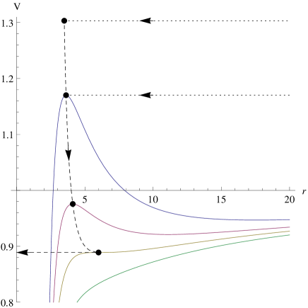
Figure 1: For Sec. III.1: Illustration of the effective potential (13) for different values of $L$. From above, the four full lines illustrate the cases $L>4$, $\sqrt{12}<L<4$, $L=\sqrt{12}$ and $L<\sqrt{12}$. Note that all these curves approach $V\to 1$ as $r\to\infty$. — For Sec. IV.1: The dashed line represents the critical solution. Its almost vertical segment represents the adiabatic phase. As illustrated by the beads, it is given by $r(t)=r_{-}(L(t)),E^{2}(t)=V_{-}(L(t))$, with $\dot{L}(t)$ determined by radiation. The horizontal segment represents the plunge phase. The two dotted lines represent orbits coming in from infinity at the critical impact parameter for different $E$, and asymptoting to the critical solution. Radiation reaction has been neglected in the approach and plunge phases, while $\dot{r}$ has been approximated as zero in the adiabatic phase. With radiation reaction, to order $\eta$ the approach and plunge phase curves bend slightly downwards, the adiabatic curve is slightly further to the right, and the kinks are slightly smoothed out. [The beads are the maxima of the potential for $L=5,4.6,3.9,\sqrt{12}$, and the lowest curve (without a maximum) corresponds to $L=3$.]

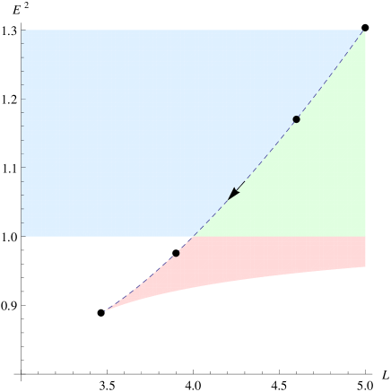
Figure 2: For Sec. III.2: The space of geodesics on Schwarzschild, labelled by angular momentum per unit mass $L$ and energy per unit mass (squared) $E^{2}$ of the particle. The bottom right shaded region contains bound orbits that oscillate between a minimum and maximum radius. Its lower edge is given by stable circular orbits. The left shaded region contains orbits that come in from infinity with low impact parameter and plunge. The top right shaded region contains orbits that come in from infinity with high impact parameter and scatter. The line dividing these two regions is therefore the threshold of immediate capture, given by $E^{2}=V_{-}(L)$ (which characterises unstable circular orbits). The white region corresponds to orbits that emerge from the white hole horizon and plunge back into the black hole, and which are not of interest to us here. — For Sec. IV.1: In the self-force approximation, the critical solution moves adiabatically along the line of unstable circular geodesic orbits, as indicated by the dashed line and arrow. The beads and arrow are as in Fig. 1. (The approach and plunge phases seen in Fig. 1 are essentially in the $r$ direction, which is suppressed here.)

The shape of the effective potential $V(L,r)$ for different ranges of $L$ is illustrated in Fig. 1. (The dashed and dotted curves should be ignored for now.) As $V(L,\infty)=1$ for any $L$, orbits with $E\geq 1$ are unbound. For $L>\sqrt{12}$, the effective potential has a maximum at $r=r_{-}$ and a minimum at $r=r_{+}$, given by

$$r_{\pm}:={L(L\pm L_{12})\over 2},$$ (20)

where it takes values

$$V_{\pm}:=V(r_{\pm})={2(2L\pm L_{12})^{2}\over 9L(L\pm L_{12})}.$$ (21)

Here we have introduced the shorthand

$$L_{12}:=\sqrt{L^{2}-12}.$$ (22)

The minimum and maximum give rise to a stable and an unstable circular orbit. These merge for $L=\sqrt{12}$, at $r_{+}=r_{-}=6$.

For trajectories coming in from infinity, and hence with $E\geq 1$, a natural parameter of the initial data is the impact parameter $b>0$, defined by

$$b:=\lim_{r\to\infty}r\sin|\varphi(r)-\varphi(\infty)|.$$ (23)

With

$${d\varphi\over dr}={L\over r^{2}\sqrt{E^{2}-V(L,r)}},$$ (24)

we find

$$E^{2}-1={L^{2}\over b^{2}}.$$ (25)

We define the (instantaneous) orbital angular frequency

$$\Omega:={d\varphi\over dt}={\dot{\varphi}\over\dot{t}}=\left(1-{2\over r}\right){L\over r^{2}E}={V_{,L}\over 2E}.$$ (26)

For both the stable and unstable circular geodesic orbits, we have

$$E = {r-2\over\sqrt{r(r-3)}},$$ (27)

$$L = {r\over\sqrt{r-3}},$$ (28)

$$\Omega = r^{-3/2}$$ (29)

We will be particularly interested in the ultrarelativistic limit $E\gg 1$, where

$$E \simeq {1\over\sqrt{3}}(r-3)^{-1/2},$$ (30)

$$L \simeq 3(r-3)^{-1/2}\simeq 3\sqrt{3}E,$$ (31)

$$\Omega \simeq {1\over 3\sqrt{3}}.$$ (32)

III.2 Critical solution

For simplicity of presentation, in the following we discuss only geodesic orbits with $E>1$ and which initially have $\dot{r}<0$ and $r>r_{-}(L)$, coming in from large $r$. If the impact parameter is fine-tuned so that $E^{2}=V_{-}(L)$, the orbit asymptotically approaches the unstable circular orbit $r=r_{-}(L)$, without ever plunging or moving back out. Orbits with the same $L$ but smaller $E$ scatter, while orbits with the same $L$ but larger $E$ plunge. Hence the critical surface in the space of initial data parameterised by $(r,E,L)$ with $\dot{r}<0$ is formed by the surface $E^{2}=V_{-}(L)$, $r>r_{-}(L)$. The space of geodesic orbits is illustrated in Fig. 2.

We define the critical impact parameter $b_{*}(E)$ by $E^{2}=V_{-}(L=L(E,b_{*}))$ and find

$$b_{*}(E)={\sqrt{27E^{4}-36E^{2}+8+E(9E^{2}-8)^{3/2}}\over\sqrt{2}(E^{2}-1)},$$ (33)

which has the well-known limits

$$b_{*}(\infty)=3\sqrt{3}$$ (34)

and $b_{*}(1)=\infty$ (every particle released from rest at infinity falls into the black hole).

III.3 Perturbations of the critical solution

The linearisation of the dynamical system (15,16) about the critical solution $r=r_{-}(L)$ is

$$\delta\ddot{r} = -{1\over 2}V_{,rr-}\delta r-{1\over 2}V_{,rL-}\delta L,$$ (35)

$$\delta\dot{L} = 0,$$ (36)

where $V_{,rr-}$ and $V_{,rL-}$ are $V_{,rr}$ and $V_{,rL}$ evaluated on the critical solution $r=r_{-}(L)$. We can decouple these equations as

$$\ddot{x} = \Gamma^{-2}x,$$ (37)

$$\dot{\delta}L = 0,$$ (38)

where

$$x := \delta r+{V_{,rL-}\over V_{,rr-}}\delta L,$$ (39)

$$\Gamma := \left(-{1\over 2}V_{,rr-}\right)^{-1/2}={L^{3/2}(L-L_{12})^{2}\over 4L_{12}^{1/2}}.$$ (40)

With $E^{2}=V_{-}(L)$ on the critical solution, we can consider $\Gamma$ also as function of $E$, but we have not been able to express $\Gamma(E)$ in closed form.

From (35,36) we see that the critical solution has exponentially growing and decaying modes $x=\exp(\pm\tau/\Gamma)$ with $\delta L=0$, and a neutral mode $\delta L=1$ with $x=0$. Hence it has precisely one growing mode, as required of a critical solution. However, in the geodesic approximation we do not have a critical solution which is a global attractor within the critical surface, but rather a line of critical solutions, to which the neutral mode is tangent.

IV Critical solution in the self-force approximation

IV.1 Qualitative discussion

Our aim is to replace the model of the binary merger as a test particle on Schwarzschild spacetime with a more realistic model that in particular incorporates radiation reaction, but which still approximates the Einstein equations as a finite-dimensional dynamical system by integrating out the radiation.

One such model is the extreme mass-ratio approximation, where the loss of energy and angular momentum are calculated to leading order in $\eta:=m/M$, where $M=1$ is the mass of a large black hole and $m$ that of the smaller object, modelled as a point particle. We shall use an adiabatic approximation, where the particle is considered to move on a geodesic with $E$ and $L$ now slowly decaying, and a force term appearing in consequence on the right-hand side of the geodesic equation. We can then still use the effective potential picture to write the equations of motion, where $E(t)$ and $L(t)$ now evolve under the effect of the radiation reaction.

In short, the critical solution sits approximately at the maximum of the potential, with $E(t)^{2}=V_{-}(L(t))+O(\eta)$ and $r(t)=r_{-}(L(t))+O(\eta)$, while that maximum itself evolves under radiation reaction, starting with the ultrarelativistic limit (31) as $r\simeq 3$ and $E\to\infty$, and ending with a plunge from $E\simeq 8/9$, $L\simeq\sqrt{12}$ and $r\simeq 6$ (see Fig. 1). Our self-force calculation suggests that infinite $E$ and $L$ occur at finite $\tau$, $t$ and $\varphi$ in the past, but as we discuss below, we cannot consistently reach $E=\infty$ within the self-force approximation.

Any initial data that are perfectly fine-tuned to the threshold of immediate merger, with arbitrarily large $E$, join the critical solution, which acts as an attractor in the critical surface. This is indicated schematically in Figs. 1 and 2, where the dotted lines with arrows indicate two fine-tuned solutions approaching the critical solution (dashed) and remaining on it until and through the plunge. Note that the line of critical fixed points in the test particle picture has become a single, adiabatically evolving critical solution.

IV.2 Equations of motion

In the extreme mass ratio limit, the larger object in the binary is approximated as a Schwarzschild black hole, and the lighter one as a particle moving in this background spacetime, with the equation of motion

$$u^{b}\nabla_{b}u^{a}=F^{a},$$ (41)

where $u^{b}\nabla_{b}u^{a}=0$ describes a geodesic on the background Schwarzschild spacetime, and $F^{a}$ is the self-force per particle rest mass, which is proportional to the mass ratio $\eta$ to leading order. (We use terminology customary in the self-force literature where it is really $mE$, $mML$ and $mF^{a}$ that have dimensions of energy, angular momentum and force.) $\nabla_{a}$ is the covariant derivative in the background spacetime, and indices are moved implicitly with the background metric.

As before, we define $E$ and $L$ by (10) and (11), and we impose the normalisation $u^{a}u_{a}=-1$ in the form (12). The time derivative of $u^{a}u_{a}=-1$ gives the usual constraint on any 4-force, namely

$$u_{a}F^{a}=0.$$ (42)

From (41), we now have the 3-dimensional dynamical system

$$\ddot{r} = -{1\over 2}V_{,r}(L,r)+F^{r},$$ (43)

$$\dot{L} = F_{\varphi}.$$ (44)

$E$ can be read off as $E(r,\dot{r},L)$ from (12), or can be evolved using the third component of (41), which can be written as

$$\dot{E}=-F_{t}.$$ (45)

These are compatible because of (42), which can be written as

$$\dot{r}F^{r}+E(F_{t}+\Omega F_{\varphi})=0,$$ (46)

where $\Omega$ is defined by (26). $\varphi$ and $t$ are evolved via (11) and (10).

IV.3 Adiabatic expansion

By definition, the critical solution is the one that is balanced between plunging and running out to infinity. In the absence of radiation reaction, this clearly means it is a circular geodesic sitting on top of the potential. In the presence of radiation reaction, this definition becomes teleological: the critical solution hesitates as long as possible between plunging and running out to infinity. In practice we use adiabaticity to define the critical solution as being as circular or as stationary as possible: $r$ should vary over a radiation reaction timescale, that is, $\dot{r}$ should be proportional to the mass ratio $\eta$ to leading order in the self-force expansion.

We formalize the adiabatic expansion through the series ansatz (slow-time expansion) HindererFlanagan

$$F^{a}_{*}(\tau) = \sum_{k=1}^{\infty}\eta^{k}F^{a}_{k}(\hat{\tau}),$$ (47)

$$r_{*}(\tau) = \sum_{k=0}^{\infty}\eta^{k}r_{k}(\hat{\tau}),$$ (48)

$$L_{*}(\tau) = \sum_{k=0}^{\infty}\eta^{k}L_{k}(\hat{\tau}),$$ (49)

$$E_{*}(\tau) = \sum_{k=0}^{\infty}\eta^{k}E_{k}(\hat{\tau}),$$ (50)

where we have defined the slow time

$$\hat{\tau}:=\eta\tau,$$ (51)

the suffix $*$ denotes the critical solution, and the normalisation condition (12) is obeyed order by order by virtue of (46). To leading order,

$$F^{a}_{*} = \eta F^{a}_{1}+O(\eta^{2}),$$ (52)

$$\ddot{r}_{*} = \eta^{2}r_{0}^{\prime\prime}+O(\eta^{3}),$$ (53)

$$\dot{L}_{*} = \eta L_{0}^{\prime}+O(\eta^{2}),$$ (54)

$$\dot{E}_{*} = \eta E_{0}^{\prime}+O(\eta^{2}).$$ (55)

where $\dot{f}:=df/d\tau$ as before, and $f^{\prime}:=df/d\hat{\tau}$. Substituting this into (43,44), we obtain to leading order [$O(1)$ in (43), and $O(\eta)$ in (44)]

$$0 = V_{,r}(L_{0},r_{0})\quad\Rightarrow\quad r_{0}=r_{-}(L_{0}),$$ (56)

$$L_{0}^{\prime} = F_{\varphi 1},$$ (57)

and this allows us to integrate $r_{0}$ and $L_{0}$. Hence, $F^{a}_{1}(\hat{\tau})=F^{a}_{1}(r_{0}(\hat{\tau}))$ is the first-order self-force on a circular geodesic orbit of radius $r_{0}$, which is known Barack:2007tm . To next order,

$$0 = -{1\over 2}[V_{,rr-}(L_{0},r_{0})r_{1}+V_{,rL}(L_{0},r_{0})L_{1}]+F^{r}_{1},$$ (58)

$$L_{1}^{\prime} = F_{\varphi 2}$$ (59)

formally give us $r_{1}$ and $L_{1}$, but we cannot use this to calculate the critical solution beyond $(r_{0},L_{0})$. $F^{a}_{2}$ is the second-order self-force. It comprises terms that are quadratic in metric perturbations and corrections due to the fact that the critical solution is not exactly geodesic. Both have not yet been calculated. Note, however, that (58) can be rewritten as

$$0=-{1\over 2}V_{,r}(L_{0}+\eta L_{1},r_{0}+\eta r_{1})+\eta F^{r}_{1}+O(\eta^{2}),$$ (60)

and so its physical meaning is that the critical solution is slightly off the peak of the geodesic potential, held there (to this order) by the conservative part $F^{r}_{1}$ of the self-force.

IV.4 Self-force input

To leading order, our analysis requires knowledge of $\dot{L}=F_{\varphi}$ along circular orbits with $3<r\leq 6$. In practice, we calculate $\dot{E}=-F_{t}$, which on circular orbits is related to $\dot{L}$ by $\dot{L}=\dot{E}/\Omega$. To obtain $\dot{E}$ we used the self-force code developed in Ref. Akcay:2010dx , which is a frequency-domain variant of the original Barack-Sago code Barack:2007tm . The code was originally developed to deal with stable orbits, but it can handle unstable (circular) orbits without any further development. The code takes as input the orbital radius $r$ and returns the value of $\dot{E}$ along that orbit. We have obtained accurate data for a dense sample of $r$ values in the range $3<r\leq 6$. The numerical data and details of their derivation are given in Appendix A.

Our numerical results can be approximated by the semi-heuristic fitting formula

$$\dot{E}\simeq-\eta r^{-5}\ z^{-\alpha}\ (a_{0}+a_{1}z+a_{2}z^{2}+a_{3}z^{3}),$$ (61)

where $z:=1-3/r$ and the parameters

$$\alpha\simeq 1.773163,\quad a_{0}\simeq 2.87683,\quad a_{1}\simeq-4.01414,$$

$$a_{2}\simeq 10.5371,\quad a_{3}\simeq-3.79087$$ (62)

have been determined by a least-squares fit of $\dot{E}$ versus $z$. The $r^{-5}$ decay at large $r$ is well-known. We have modelled the blow-up of the self-force at the light ring by a single power $z^{-\alpha}$, although we have no rigorous theoretical argument for this. The numerical data we have fitted to are also not very close to the light ring, with the smallest value of $r$ at $3.02$, corresponding to $E\simeq 4.15$.

A tentative theoretical argument for determining $\alpha$ is that at sufficiently high energy the metric perturbation should be proportional to the total energy $E$ of the particle and therefore the fluxes as seen by an observer at rest should be proportional to $E^{2}$, so that

$$\dot{E}\sim\dot{t}\,E^{2}\sim z^{-3/2}.$$ (63)

[Note that, from (10) and (27), $\dot{t}=z^{-1/2}$ on circular geodesics.] A least-squares fit to (61) where $\alpha=1.5$ is held fixed results in a maximum fitting error of $17\%$. By comparison, the maximum fitting error with (62) is $0.5\%$, which is much smaller and comparable with the maximal estimated error of the self-force calculation (see Appendix A). The numerical self-force results and both fits are shown in Fig. 3. For our computations and plots in the remainder of the paper, we shall use the fit (61) with (62) for the range $r\geq 3.02$ for which we have self-force data, corresponding to $E\lesssim 4.15$.

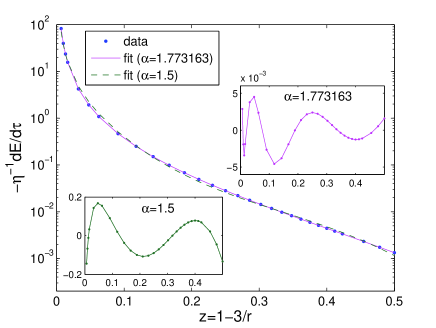
Figure 3: Energy loss $\dot{E}/\eta$ as a function of $z:=1-3/r$, for a circular geodesic orbit in the self-force approximation, and two closed-form fits. The fitting ansatz is given by Eq. (61) with $\alpha$ either fitted (solid line), or fixed at $\alpha=3/2$ (dashed line). The self-force data (points) are given in Appendix A. The insets show the relative differences between the fit and the data for the two models (note the different vertical scales).

Fig. 4 shows the energy absorbed by the large black hole as a fraction of the total energy loss (radiated to infinity plus absorbed by the large black hole). This figure is relevant for computing the total energy radiated to infinity, but not for our construction of the critical solution, where only the total energy loss matters.

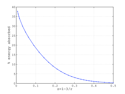
Figure 4: The fraction of the total energy loss $\dot{E}/\eta$ that is absorbed by the large black hole, as a function of $z:=1-3/r$. This is based on the data in Appendix A. Extrapolation gives a fraction of $\simeq 42\%$ at the light ring itself.

IV.5 Integration of the critical solution

In the presence of radiation reaction, for a given mass ratio $\eta$, there is a single critical solution where $E$, $L$, $\Omega$, $r$, $\tau$ and $\varphi$ are all monotonous functions of one another, with $E$ and $L$ decreasing from $\infty$ to finite values at plunge, $r$ increasing from $3$ to $6$, and $\Omega$ decreasing from $3^{-3/2}$ to $6^{-3/2}$, all as $\tau$ and $\varphi$ increase. In this paper we construct the critical solution only to leading order in $\eta$. Then $E$, $L$ and $\Omega$ and $r$ are known functions of one another, related by (27-29). Furthermore, the $\eta$-dependence of the critical solution is of the simple form $r=r(\hat{\tau})=r(\hat{\varphi})$, where we define the “slow angle”

$$\hat{\varphi}:=\eta\varphi$$ (64)

in analogy to the slow time $\hat{\tau}$. Finally, the ODEs obeyed by $\hat{\tau}(r)$ and $\hat{\varphi}(r)$ are separable, and can be solved by integration.

We obtain ${\hat{\varphi}}(r)$ by (numerical) integration of

$${d{\hat{\varphi}}\over dr} = \eta{d\varphi\over dt}{dt\over d\tau}{d\tau\over dE}{dE\over dr}=\Omega\dot{t}{dE\over dr}{\eta\over\dot{E}}$$ (65)

$$= {1\over 2}r^{-5/2}(r-3)^{-2}(r-6){\eta\over\dot{E}},$$

after substituting (61). A very good closed form approximation to this integral in terms of elementary functions can be obtained by approximating $(d\hat{\varphi}/dr)/(r-6)$ as a series in $(r-3)$ with three terms, multiplying back by $(r-6)$, and integrating this. The full result, the closed form approximation, and the ultrarelativistic approximation discussed below are shown in Fig. 5. For fixed $\eta$, this graph gives us the shape of the critical orbit.

We only have reliable self-force data for $r\geq 3.02$, corresponding to $E\lesssim 4.15$, but we are interested in the critical solution up to $E=\infty$. We have therefore extrapolated our fit (61) with (62) down to $r=3$ in producing Fig. 5, and have used this extrapolation to set $\hat{\varphi}(3)=0$ at $E=\infty$ as a matter of convention. Note, however, that almost the entire range of $\hat{\varphi}$ in this plot occurs for $r>3.02$, where we do have reliable self-force data, with $\hat{\varphi}(3.02)\simeq 0.07$ compared to $\hat{\varphi}(6)\simeq 2.6$. This qualitative feature is robust, requiring only that $\dot{E}$ diverges at the light ring faster than $(r-3)^{-1}$, that is $\alpha>1$. Our self-force data for $r\leq 3.02$ support this qualitative feature robustly, with $\alpha\simeq 1.77$, while our crude theoretical model suggests $\alpha=3/2$.

Hence, the total number of orbits in the critical solution, from infinite energy down to plunge, is given by

$$n_{\rm tot}={\hat{\varphi}(6)\over 2\pi\eta}\simeq{0.41\over\eta},$$ (66)

and we expect the numerical prefactor to depend only weakly on our extrapolation of the self-force data.

We obtain $\hat{\tau}(r)$ by (numerical) integration of

$${d\hat{\tau}\over dr}={\eta\over\dot{E}}{dE\over dr}.$$ (67)

A reasonably good closed form approximation for $\hat{\tau}(r)$ can be obtained by expanding $(d\hat{\tau}/dr)/(r-6)$ into a series in $(r-3)$ with four terms, multiplying back by $(r-6)$, and integrating. The full result and its approximations are shown in Fig. 6. Our self-force data suggest that $\hat{\tau}$, too, is finite at infinite energy, and we use the convention that $\hat{\tau}=0$ at $E=\infty$. [From (67,30), the precise criterion is that $(r-3)^{-3/2}/\dot{E}$ is integrable.] Again, compare $\hat{\tau}(3.02)\simeq 0.02$ with $\hat{\tau}(6)\simeq 9.62$.

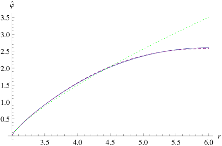
Figure 5: Slow angle $\hat{\varphi}$ as a function of radius $r$ in the critical solution. We have fixed $\hat{\varphi}=0$ at $r=3$. The full line represents a numerical integration of (65), with $\dot{E}(r)$ given by the fitting formula (61). The dashed line represents the closed form approximation discussed in the text below Eq. (65), and the dotted line the ultrarelativistic approximation (69). Note that here and in the following figure, the narrow section $r<3<3.02$ of the domain is derived from an extrapolation of our self-force data.

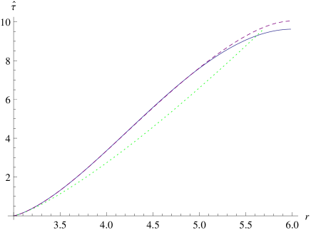
Figure 6: Slow time $\hat{\tau}$ as a function of radius $r$ in the critical solution. We have fixed $\hat{\tau}=0$ at $r=3$. The full line represents a numerical integration of (67). The dashed line represents the closed form approximation for $\hat{\tau}(r)$ discussed in the text below Eq. (67) and the dotted line the ultrarelativistic approximation (70).

IV.6 The ultrarelativistic approximation

In order to make quantitative statements about the critical solution beyond the energies covered by our self-force data, we shall assume that as $E\to\infty$, $\dot{E}$ diverges like the leading order of (61), that is

$${\dot{E}\over\eta}\simeq-3^{\alpha-5}a_{0}(r-3)^{-\alpha}.$$ (68)

(As discussed above, our qualitative conclusions that $\hat{\varphi}$ and $\hat{\tau}$ are finite at $E=\infty$ depend only on $(r-3)^{-2}/\dot{E}$ and $(r-3)^{-3/2}/\dot{E}$ being integrable as $r\to 3$.) We shall refer to calculations where we only use the leading power of $(r-3)$ throughout as the ultrarelativistic approximation, and in this context we shall treat $a_{0}>0$ and $\alpha>1$ as undetermined.

Combining the leading order of (65) with (68) and integrating, we obtain

$$\hat{\varphi}(r)\simeq{3^{7/2-\alpha}\over 2a_{0}(\alpha-1)}(r-3)^{\alpha-1},$$ (69)

Similarly, taking the leading power of $(r-3)$ in (67), we obtain

$$\hat{\tau}(r)={3^{9/2-\alpha}\over a_{0}(2\alpha-1)}(r-3)^{2\alpha-1\over 2}.$$ (70)

In the ultrarelativistic approximation we can combine (30) with (69) and (70) to express $r-3$, $\hat{\tau}$, $\hat{\varphi}$ and $E$ all as powers of each other. In particular

$$E(\hat{\tau})\simeq C_{E}\hat{\tau}^{-\beta},$$ (71)

where

$$C_{E}:=[3^{2\alpha-5}a_{0}(2\alpha-1)]^{-\beta},\qquad\beta:={1\over 2\alpha-1}$$ (72)

which will be used later. With

$$\dot{\varphi}\simeq{E\over\sqrt{3}}$$ (73)

in the ultrarelativistic approximation, we also have

$$\hat{\varphi}\simeq{C_{E}\over\sqrt{3}(1-\beta)}\hat{\tau}^{1-\beta}\simeq{C_{E}^{1/\beta}\over\sqrt{3}(1-\beta)}E^{1-1/\beta}.$$ (74)

In the ultrarelativistic limit (40) becomes

$$\Gamma\simeq{9\over L}\simeq{\sqrt{3}\over E}\simeq{\sqrt{3}\over C_{E}}\hat{\tau}^{\beta},$$ (75)

where we have used (71) in the last equality.

IV.7 Validity of the self-force and adiabatic approximations

The self-force approximation to the equations of motion is valid when the total energy $mE$ of the small object is much smaller than the total energy $M$ of the large black hole, that is, for

$$E\ll\eta^{-1}.$$ (76)

Because the self-force diverges as $E\to\infty$ at fixed $\eta$, we must also estimate where the adiabatic approximation breaks down at high energy. Heuristically, we assume that the adiabatic approximation is valid if $E$ changes at most by some small fraction $\delta\ll 1$ per orbit, or

$$-{d\ln E\over d\hat{\varphi}}\ll{\delta\over 2\pi\eta}.$$ (77)

(The explicit $\eta$ on the right comes from the hat on the left.) From (74), we find that in the ultrarelativistic regime this is equivalent to

$$E\ll\left({\eta\over\delta}\right)^{-{1\over 2\alpha-2}}.$$ (78)

We see that the adiabaticity condition (78) always implies the condition (76) for the self-force approximation itself to be valid if $\alpha\geq 3/2$. (Recall our theoretically motivated value of $\alpha$ is $3/2$, and our fitted value is $1.77$.)

Note that the adiabatic approximation breaks down also as the plunge is approached, because the effective potential becomes shallower, leading to a rapid increase in $r_{1}$ at finite $F^{r}$ in (58) OriThorne .

V Critical scaling in the self-force approximation

V.1 Perturbations of the critical solution

We now consider a small perturbation of the critical solution that results from imperfect fine-tuning of the initial data, as discussed above in Sec. II, namely

$$r=r_{*}(\hat{\tau})+\delta r(\tau),\qquad L=L_{*}(\hat{\tau})+\delta L(\tau),$$ (79)

where $r_{*}$ and $L_{*}$ are given by the adiabatic ansatz (48,49) above, while $\delta r$ and $\delta L$ are just functions of $\tau$, that is, they are assumed to remain “fast” even in the limit of weak radiation reaction. The self-acceleration is perturbed as

$$F^{a}=F^{a}_{*}+O(\eta)O(\delta r,\delta L),$$ (80)

where the factor $\eta$ arises simply because any self-acceleration scales as $O(\eta)$. Substituting this into the equations of motion and subtracting the critical solution, we formally obtain

$$\delta\ddot{r} = -{1\over 2}[V_{,rr-}(L_{0},r_{0})\delta r+V_{,rL}(L_{0},r_{0})\delta L]$$ (81)

$$+O(\delta r^{2},\delta L^{2},\delta r\delta L)+O(\eta)O(\delta r,\delta L),$$

$$\delta\dot{L} = O(\eta)O(\delta r,\delta L).$$ (82)

We now neglect the error terms above, the first set as they are nonlinear in $(\delta r,\delta L)$, the second set as they are small corrections to the coefficients of a linear differential equation for $(\delta r,\delta L)$.

In identifying the perturbed solution with the background critical solution, we can adjust the origin of $\tau$ in the perturbed solution. (This is a remnant of the usual gauge-dependence of spacetime perturbations.) As $L_{*}(\hat{\tau})$ is not constant, we can use this to set $\delta L=0$ at any one time, and hence, by $\delta\dot{L}\simeq 0$, at all times. Note that the neutral mode $\delta L=\rm constant$ present in the geodesic approximation, which linked neigbouring critical solutions, has become a gauge mode in the presence of radiation reaction, where there is a single critical solution, and that we have used a simple form of gauge fixing to eliminate this mode. From now on we denote $\delta r$ in this gauge by $x$. We are left with the single equation of motion

$$\ddot{x}\simeq\Gamma(\hat{\tau})^{-2}x,$$ (83)

which is equivalent to (37) for the geodesic case, but where now

$$\Gamma(\hat{\tau}):=\Gamma[L_{0}(\hat{\tau})]$$ (84)

is time-dependent.

Rewriting the equation entirely in terms of $\hat{\tau}$, we have

$$x^{\prime\prime}\simeq\eta^{-2}\Gamma(\hat{\tau})^{-2}\ x,$$ (85)

where as before a prime denotes $d/d\hat{\tau}$. As $\eta$ is small, we can use a WKB approximation. In terms of the “WKB time”

$$T(\hat{\tau}):=\int{d\hat{\tau}\over\Gamma(\hat{\tau})},$$ (86)

where for definiteness we let $T(0)=0$, the first-order WKB approximation to the growing and decaying solutions is

$$x_{\pm}(\hat{\tau})\simeq\sqrt{\Gamma(\hat{\tau})}e^{\pm\eta^{-1}T(\hat{\tau})}.$$ (87)

This is a good approximation for $|\dot{\Gamma}|\ll 1$, when the prefactor varies much more slowly than the exponential. The functions $\Gamma(\hat{\tau})$ and $T(\hat{\tau})$ are shown in Figs. 7 and 8.

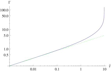
Figure 7: Log-log plot of $\Gamma(\hat{\tau})$ [defined in (40], based on (61,62) (solid line), and the ultrarelativistic approximation (75) (dotted line). (The divergence of $\Gamma$ comes from the shallowness of the potential at $r=6$.)

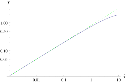
Figure 8: Log-log plot of $T(\hat{\tau})$ [defined in (86], based on (61,62) (solid line), and the ultrarelativistic approximation (88) (dotted line).

In the ultrarelativistic approximation, from (75), we have

$$T\simeq{C_{E}\over\sqrt{3}(1-\beta)}\hat{\tau}^{1-\beta}\simeq{C_{E}^{1/\beta}\over\sqrt{3}(1-\beta)}E^{1-1/\beta}\simeq\hat{\varphi},$$ (88)

where we have used (74) in the last two equalities. In the same approximation,

$$\dot{\Gamma}\simeq\sqrt{3}\beta C_{E}^{1-2\alpha}\eta E^{2\alpha-2}.$$ (89)

Hence $|\dot{\Gamma}|\ll 1$ for

$$E\ll\eta^{-{1\over 2\alpha-2}},$$ (90)

which has the same power of $\eta$ as the criterion (78) for the critical solution to evolve adiabatically. Clearly, with $\delta<1$, (78) implies (90) and hence, for $\alpha\geq 3/2$, also (76). Hence the only criterion we need to impose is (78) (the critical solution evolves adiabatically), and we can then always use the WKB approximation to the critical solution.

For $\tau$ small enough ($E$ large enough) that $|\dot{\Gamma}|\gg 1$, the WKB approximation does not hold. However, we are then necessarily in the ultrarelativistic limit such that the approximation (75) for $\Gamma(\hat{\tau})$ holds, and with this, (83) can be solved in closed form in terms of Bessel functions. As this result is not directly relevant for our main result, we give it in Appendix B.

V.2 Dependence on the initial data

For definiteness, we parameterise the space of initial data (modulo a shift in time) by the initial energy at infinity $E_{i}$ and the impact parameter $b$. We consider a generic near-critical solution in the whirl phase $\tau_{i}<\tau<\tau_{f}$ where it is close to the critical solution, so that

$$x(\tau)\simeq A(E_{i},b){x_{-}(\tau)\over x_{-}(\tau_{i})}+B(E_{i},b){x_{+}(\tau)\over x_{+}(\tau_{i})}.$$ (91)

The factors $x_{\pm}(\tau_{i})$ have been introduced for later convenience.

$A$ and $B$ are smooth functions of $E_{i}$ and $b$, and by definition $B$ vanishes for critical initial data. Therefore,

$$A=A_{0}(E_{i})+O(\delta b),\quad B=B_{1}(E_{i})\delta b+O(\delta b)^{2},$$ (92)

where

$$\delta b:=b-b_{*}(E_{i},\eta).$$ (93)

[The critical value $b_{*}(E_{i},\eta)$ of the impact parameter is known in closed form only for $\eta=0$, when it is given by (33), but its value does not matter in the following.] We must have $A>0$ and $B_{1}>0$ because $x$ is positive and decreasing during the approach to the critical solution, and then becomes negative in the capture case $b<b_{*}$, or returns to large positive values in the scattering case $b>b_{*}$.

Let the beginning and end of the whirl phase be defined by $x(\tau_{i})=X_{i}$ and $x(\tau_{f})=X_{f}$, where $X_{i}$ and $X_{f}$ will be characterised later. If the whirl phase is sufficiently long, we can neglect the growing mode at $\tau_{i}$ and the decaying mode at $\tau_{f}$, so that

$$A_{0} \simeq X_{i},$$ (94)

$$B_{1}\delta b \simeq X_{f}{x_{+}(\tau_{i})\over x_{+}(\tau_{f})}.$$ (95)

Note that $X_{i}$ is always positive, while $X_{f}$ is positive for initial data that scatter and negative for initial data that plunge.

In the general discussion of critical scaling in Sec. II, we introduced two constants $C_{1}$ and $C_{2}$ that were treated as unknown, and combined into a constant $C_{3}$ in the final result (4). The equivalents of $C_{1}$ and $C_{2}$ in the current specific problem are $B_{1}$ and $X_{f}$, respectively, and we shall now see that under certain conditions we can determine both, so that there is no undetermined constant left in our final results.

In order to determine $B_{1}$ we can use an energy argument if we approximate $E$ as constant during the approach phase. This is justified when the energy loss during the approach phase is small compared to the energy loss during an extended whirl phase. We approximate (87) over a short time interval (covering the transition from approach to whirl) as

$$x_{\pm}(\tau)\simeq e^{\pm(\tau-\tau_{i})/\Gamma(\tau_{i})}x_{\pm}(\tau_{i}).$$ (96)

Perturbing (12), which holds for geodesics, with respect to $b$, we obtain

$$E^{2}(L,b)-E_{*}^{2}(L)\simeq\dot{x}^{2}-\Gamma^{-2}x^{2}\simeq-4\Gamma^{-2}AB,$$ (97)

where the last equality follows from (96). This equation becomes exact in the geodesic limit, where $E$ is conserved and (96) is exact. On the other hand, when $E$ is conserved, from (25) we also have

$$E^{2}(L,b)-E_{*}^{2}(L)\simeq-{2L^{2}\over b_{*}^{3}}\delta b\simeq-2[E_{*}^{2}(L)-1]{\delta b\over b_{*}}.$$ (98)

Note the factor $E^{2}-1$ in $dE/db$. It comes about because geodesic orbits with $E=1$ are at rest at infinity, and so the impact parameter is not defined. More concretely, displacing a particle at rest at infinity in a direction orthogonally to the line of sight to the large black hole before dropping it corresponds to a rotation of the binary system and makes no difference to the infall. Because of this factor, some of our following results will be formally singular at $E=1$. This is only because $b$ becomes a bad parameter of the initial data. In practice, we are interested in initial data with $E>1$ (and in particular $E\gg 1$), when this is not a problem.

We now approximate $E_{*}(L)=E_{i}$ in (98) and $\Gamma\simeq\Gamma[L_{*}(E_{i})]=:\Gamma_{i}$ in (97) because we approximate $E$ and $L$ as constant for $\tau<\tau_{i}$ and because $L_{i}\simeq L_{*}(E_{i})$ by fine-tuning. Hence we find

$$A_{0}B_{1}\simeq{\Gamma_{i}^{2}(E_{i}^{2}-1)\over 2b_{*}}.$$ (99)

From (94), (95) and (99), and taking the logarithm for later convenience, we now obtain

$$-\ln{|\delta b|\over b_{*}}-\ln\left|{\Gamma_{i}^{2}(E_{i}^{2}-1)\over 2X_{i}X_{f}}\right|\simeq\ln{x_{+}(\tau_{f})\over x_{+}(\tau_{i})}.$$ (100)

This is our master equation for critical scaling: in principle, it determines $E_{f}$ in terms of the mass ratio $\eta$ and the initial data $(E_{i},b)$. In order to obtain a definite result, however, we still need to fix $X_{i}$ and $X_{f}$. As we discuss below, there is a natural criterion for fixing them in the radiation reaction, but only a more arbitrary one in the geodesic limit. Moreover, the criterion we choose in the radiation reaction case has a singular limit as $\eta\to 0$ in the geodesic limit. We therefore discuss both cases separately, starting with the geodesic case.

V.3 Critical exponents in the geodesic case

The critical solution is by definition as circular as possible in the presence of radiation reaction, sitting approximately at the top of the potential. Hence one possible criterion for $X_{i}$ and $X_{f}$ is that the radial velocity be a given small fraction $C_{e}$ (for “eccentricity”) of the tangential velocity, or

$$\left({|\dot{x}|\over r\dot{\varphi}}\right)_{i,f}=C_{e}.$$ (101)

Note that $C_{e}$ plays the role of $C_{2}$ in our general discussion in Sec. II, and while it must be small, its choice is arbitrary – we have introduced it here because it is more intuitive than $X_{i,f}$. We have

$$\left({|\dot{x}|\over r\dot{\varphi}}\right)_{i,f}\simeq{\sqrt{E^{2}-V}\over r^{-1}L}\simeq{|X_{i,f}|\over\Gamma r^{-1}L}\simeq{|X_{i,f}|\over\sqrt{3}\Gamma E},$$ (102)

where we have used (11) and (12) in the first step, (40) in the second step, and the third approximation holds only in the ultrarelativistic limit.

In the geodesic case, where the background solution is time independent,

$$x_{\pm}=e^{\pm\tau/\Gamma}$$ (103)

holds exactly. Using this and (100-102), we obtain

$$\tau_{f}-\tau_{i}\simeq-\Gamma\ln{|\delta b|\over b_{*}}-\Gamma\ln\tilde{C}_{e}.$$ (104)

were $\Gamma$ is given by (40). Here

$$\tilde{C}_{e}:={E^{2}-1\over 2C_{e}^{2}r^{-2}L^{2}}={4-r\over 2C_{e}^{2}r}\simeq{1\over 6C_{e}^{2}},$$ (105)

where the last approximate equality holds only in the ultrarelativistic limit $r\simeq 3$. Clearly, $\tilde{C}_{e}$ inherits the arbitrariness of $C_{e}$. The result (104) can be expressed in terms of orbits as

$$n\simeq-\gamma\ln{|\delta b|\over b_{*}}-\gamma\ln\tilde{C}_{e},$$ (106)

where

$$\gamma:={\dot{\varphi}\over 2\pi}\Gamma={L^{1/2}\over 2\pi L_{12}^{1/2}}$$ (107)

In the ultrarelativistic limit, we have

$$\Gamma \simeq {\sqrt{3}\over E},$$ (108)

$$\gamma \simeq {1\over 2\pi}.$$ (109)

The critical exponents $\Gamma$ and $\gamma$ for the geodesic limit were previously obtained by Pretorius and Khurana PretoriusKhurana for equatorial geodesics of Kerr, and had previously been given, in different notation, in Eq. (2.25) of CutlerKennefickPoisson . The additive constant parameterised by $C_{e}$ could only be determined more exactly by a full modelling of the perturbed orbit to replace the artifical split into a zoom-in, whirl and zoom-out or plunge phase.

As an extension of the result for the time spent whirling, we can – trivially – estimate the energy loss during the whirl phase as

$$\Delta E\simeq(\tau_{f}-\tau_{i})\dot{E}(E_{i}),$$ (110)

where $(\tau_{f}-\tau_{i})$ is given in terms of the initial data by (104) and the constant $\dot{E}(E_{i})$ is given implicitly by relating $E_{i}$ to $r$ using the exact formula (27) for the energy on a circular orbit and $\dot{E}$ to $r$ using our numerical result (77) for the energy loss on circular geodesics. This approximation, where we neglect the radiation reaction on the orbit itself, is therefore consistent only for $\Delta E\ll E_{i}$. (110) complements the results given in Bertietal2010 for the energy radiated in the geodesic approximation scattering orbits not close to the threshold of immediate merger.

V.4 Generalised critical scaling in the radiation reaction case

With radiation reaction, a less arbitrary definition of $X_{i}$ and $X_{f}$ is given by equating the rate of change of the perturbation $x$ with that of the background solution, that is

$$|\dot{x}|\simeq|\Gamma_{i,f}X_{i,f}|\simeq\dot{r}_{*}.$$ (111)

Furthermore, we have seen above that we can always use the WKB approximation (87) to the perturbation modes when the adiabatic self-force approximation to the background critical solution is valid. Substituting our new definition (111) of $X_{i,f}$ into the left-hand side of the scaling master equation (100), and the WKB approximation (87) into its right-hand side, (100) becomes

$$-\ln{|\delta b|\over b_{*}}-\ln{\Gamma_{i}^{3}\Gamma_{f}(E_{i}^{2}-1)\over 2\eta^{-2}r_{0i}^{\prime}r_{0f}^{\prime}}\simeq{T_{f}-T_{i}\over\eta}+{1\over 2}\ln{\Gamma_{f}\over\Gamma_{i}}.$$ (112)

We can re-order this as

$$-\ln{|\delta b|\over b_{*}}\simeq{T_{f}-T_{i}\over\eta}+2\ln\eta+K_{i}+K_{f},$$ (113)

where we have defined the shorthands

$$K_{i} := \ln{\Gamma_{i}^{5/2}(E_{i}^{2}-1)\over 2r_{0i}^{\prime}},$$ (114)

$$K_{f} := \ln{\Gamma_{f}^{3/2}\over r_{0f}^{\prime}}.$$ (115)

Here we consider $T$, $K_{i}$ and $K_{f}$ as functions of $\hat{\tau}$ (or any of the other slow variables $E$, $r$, $\hat{\varphi}$). The only $\eta$-dependence is then the one explicitly shown in (113).

Alternatively, we can re-order (113) as

$${T_{f}\over\eta}+K_{f}\simeq-\ln{|\delta b|\over b_{*}}+{\hat{T}_{i}\over\eta}-K_{i}-2\ln\eta.$$ (116)

This gives a known function of $\hat{\tau}_{f}$ (or $E_{f}$), on the left-hand side, as a known function of the mass ratio $\eta$ and the initial data $(E_{i},b_{i})$, on the right-hand side. To fully expand this in terms of $E_{f}$ and $E_{i}$, we first note that (27) gives an expression for $E(r)$ that can be inverted to obtain $r(E)$. (40) gives $\Gamma(L)$ and (28) gives $L(r)$, so that we can explicitly obtain $\Gamma(E)$. (We do not give the expression here, as it is unwieldy.) Next we note that (67) can be rewritten as

$$r_{0}^{\prime}(r)=[\eta^{-1}\dot{E}](r)\left({dE\over dr}\right)^{-1},$$ (117)

where $r_{0}^{\prime}:=dr_{0}/d\hat{\tau}$ as before. Finally we note that the definition (86) of $T(\hat{\tau})$ can be rewritten as

$$T(r)=\int{dr\over r_{0}^{\prime}(r)\Gamma(r)},$$ (118)

which can then be written as $T(r(E))$, or directly as

$$T(E)=\int{dE\over r_{0}^{\prime}(r(E))\Gamma(r(E)){dE\over dr}(r(E))}.$$ (119)

With the definitions (114,115) of $K_{i}$ and $K_{e}$ in terms of $\Gamma$, $E$ and $r_{0}^{\prime}$, we can now write our master equation (116) in terms of the mass ratio $\eta$, the initial data $(E_{i},b)$, and the final energy $E_{f}$, subject to evaluating the integral in either (118) or (119). However, this equation cannot be solved for $E_{f}=E_{f}(\eta,E_{i},b)$ in closed form.

We can make (116) more explicit, in terms of only powers and logarithms, when the entire whirl phase is ultrarelativistic, that is $E_{f}\gg 1$. We have already given the ultrarelativistic approximations for $T(\hat{\tau})$, $\hat{T}(E)$ and $T(\hat{\varphi})$ in (88), and we similarly find that that in the ultrarelativistic limit

$$K_{i} \simeq -2\ln 2+\left({3\over 4}+6\beta\right)\ln 3$$ (120)

$$-{3\beta\over 2}\ln a_{0}+\left(1-{3\beta\over 2}\right)\ln{\hat{\tau}\over\beta},$$

$$K_{f} \simeq -\ln 2+\left({5\over 4}+2\beta\right)\ln 3$$ (121)

$$-{\beta\over 2}\ln a_{0}+\left(1-{\beta\over 2}\right)\ln{\hat{\tau}\over\beta}.$$

[These can be readily re-expressed in terms of $\hat{\varphi}$, $E$, or $(r-3)$ using (69-71).] We have plotted $T(\hat{\tau})$ above in Fig. 8, and we plot $K_{i}(\hat{\tau})$ and $K_{f}(\hat{\tau})$ in Figs. 9 and 10, all based on (61,62) and each compared against its ultrarelativistic approximation. Fig. 11 plots all three against $E$ instead of $\hat{\tau}$.

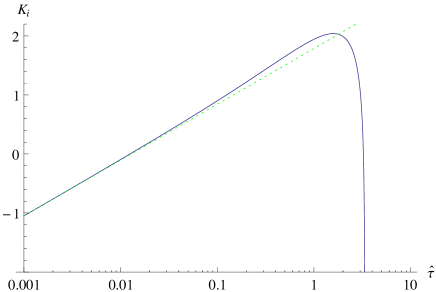
Figure 9: Log-linear plot of $K_{i}(\hat{\tau})$ [defined in (114], based on (61,62) (solid line), and the ultrarelativistic approximation (120) (dotted line). The full curve ends because of the factor $E^{2}-1$ in the exact expression, which is approximated as $E^{2}$ in the ultrarelativistic expression

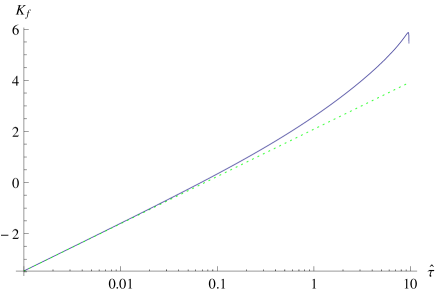
Figure 10: Log-linear plot of $K_{f}(\hat{\tau})$ [defined in (115], based on (61,62) (solid line), and the ultrarelativistic approximation (121) (dotted line).

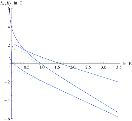
Figure 11: Plot of (from top to bottom at large $E$) $K_{i}$, $K_{f}$ and $\ln T$ (note the logarithm), all versus $\ln E$, based on (61,62) (solid lines), and the corresponding ultrarelativistic approximations (dotted lines).

Note from Fig. 11 that $\ln T$, $K_{i}$ and $K_{f}$ vary comparably rapidly along the critical solution, but it is $T/\eta$ (without the logarithm), $K_{i}$ and $K_{f}$ that appear in our scaling result (113). Hence one can suppress $K_{i}$ and $K_{f}$ in (113) as logarithmic corrections relative to the $T$ terms. Doing this, suppressing also the constant term $2\ln\eta$, and taking the ultrarelativistic limit for clarity reduces (113) to

$$-\ln{|\delta b|\over b_{*}} \simeq {T_{f}-T_{i}\over\eta}$$ (122)

$$\simeq \eta^{-\beta}{C_{E}\over\sqrt{3}(1-\beta)}\left(\tau_{f}^{1-\beta}-\tau_{i}^{1-\beta}\right)$$ (123)

$$\simeq \eta^{-1}{C_{E}^{1/\beta}\over\sqrt{3}(1-\beta)}\left(E_{f}^{1-1/\beta}-E_{i}^{1-1/\beta}\right)$$ (124)

$$\simeq \varphi_{f}-\varphi_{i}.$$ (125)

It is interesting to note that the amount of fine-tuning of the initial data (measured by $\ln|\delta b|$) required to achieve a given number of orbits on the critical solution is independent (within the self-force approximation) of the mass-ratio $\eta$. [In particular, the limit $\eta\to 0$ of (125) is trivial and gives (106) with (109).] By comparison, better fine-tuning (smaller $|\delta b|$) is required to achieve a given time on the critical solution, or a given amount of energy radiated, as $\eta$ becomes smaller. These scalings with $\eta$ are not immediately intuitive.

Finally, to see how the self-force result is related to the geodesic limit, we go back to (112). The second term on the left-hand side comes from the criterion (111) for determining $X_{i}$ and $X_{f}$, and is simply not defined when the self-force is neglected. (Formally, it diverges as $\eta\to 0$.) In the geodesic case we therefore adopted the more ad-hoc definition (101) of $X_{i}$ and $X_{f}$. Hence, in the geodesic limit the left-hand side of (112) becomes $-\ln(|\delta b|/b_{*})$ plus some constant related to $X_{i}$ and $X_{f}$ but independent of $\delta b$. On the right-hand side of (112), we note $\Gamma_{i}=\Gamma_{f}=:\Gamma$, so the second term vanishes, and from (86) we have

$$\lim_{\eta\to 0}{T_{f}-T_{i}\over\eta}={\tau_{f}-\tau_{i}\over\Gamma}.$$ (126)

Hence we recover (104) as the $\eta\to 0$ limit of (112), but with the constant $\tilde{C}_{e}$ undetermined by (112).

VI Conclusions

Pretorius and Khurana PretoriusKhurana suggested equatorial zoom-whirl orbits in Kerr as a toy model for the critical phenomena at the threshold of immediate merger in equal mass black hole binaries that they had observed in numerical relativity simulations. Here, we have adapted this toy model to make quantitative predictions in the limit where one of the two black holes is much larger than the other. We can then model the smaller black hole as a point particle of mass $m$ in a background spacetime given by the larger one (assumed to be Schwarzschild with mass $M=1$), and moving on an orbit determined by a gravitational self-force proportional, to leading order, to the mass ratio $\eta:=m/M\ll 1$.

In our model there is a single critical solution that evolves adiabatically along the sequence of unstable circular geodesics, beginning with infinite energy and ending with a plunge when almost all the energy has been dissipated in gravitational waves. In this process, the critical orbit evolves from $r=3$ and $E=\infty$ (the light ring) to $r=6$ and $E=\sqrt{8/9}$ (the last stable circular orbit), making only a finite number (approximately $0.41/\eta$) of orbits.

Any initial data fine-tuned to the critical impact parameter are attracted to the critical solution, joining it at the appropriate energy. They leave it after a number of orbits determined by the degree of fine-tuning, to either plunge or scatter. Beyond a certain degree of fine-tuning, they stay on the critical solution until it plunges.

The type of critical solution we have described here is unfamiliar in general relativity, being neither self-similar (type II) nor stationary (type I). Rather, it avoids immediate plunge or scatter by remaining as circular as is compatible with radiation reaction. The appropriate symmetry ansatz is therefore a formal slow time expansion, in which the orbit evolves adiabatically from one circular geodesic orbit to an adjacent one under the effect of energy and angular momentum loss. We might call this type Ia, for “adiabatic”.

The fact that a type Ia critical solution evolves because of dissipation makes no essential difference to the dynamical systems picture, where the critical solution is defined as balanced between two basins of attraction. The conjecture in HealyLevinShoemaker that “zoom-whirl behaviour has better odds at surviving dissipation [for smaller $\eta$] because of the slower dissipation time” is not supported by this picture, and in fact Eq. (125) shows that the dependence of the whirl angle on the fine-tuning of the initial data is independent of $\eta$ in the ultrarelativistic limit.

Our main result links the final energy (per rest mass) $E_{f}$ of the small object to its initial energy $E_{i}$, the impact parameter $b$ and the mass ratio $\eta$. This is given in implicit form in our master equation (116) – see also the discussion in the paragraph following this equation. We have also given more explicit approximate expressions (neglecting subleading terms, and assuming for clarity that $E_{f}\gg 1$) in Eqs. (123-125).

For the purpose of our calculation, there are four different regimes for the initial energy:

1) For $\sqrt{8/9}<E_{i}\lesssim 4$ we have accurate self-force data and so our results are reliable, but cannot be expressed in closed form. (We plot them, and the interested reader could reconstruct all our plots from the data and formulas given in this paper.) Even in this regime, we had to extend previous self-force calculations much closer to the light ring at $r=3M$, and it is clear that the self-force diverges there. It would be highly interesting in its own right to understand the origin of this divergence rigorously.

2) For $4\lesssim E_{i}\lesssim\eta^{-1/(2\alpha-2)}$, we are extrapolating our numerical self-force data for $\dot{E}$ as $(r-3)^{-\alpha}$, see Eq. (68). (A best fit to our numerical data gives $\alpha\simeq 1.77$, but we also have a heuristic theoretical argument for $\alpha=3/2$, which is a less good fit but not obviously wrong, see Fig. 3.) In this regime the motion is ultrarelativistic, which allows us to give explicit expressions. As $\eta$ can be arbitrarily small, we give our (extrapolated) results up to $E_{i}=\infty$.

3) If $\alpha<3/2$, there is an the even higher energy regime $\eta^{-1/(2\alpha-2)}\lesssim E_{i}\lesssim\eta^{-1}$ when the self-force approximation is still valid, but the adiabatic approximation is not. (This regime is empty for $\alpha\geq 3/2$.) It should be possible to calculate in this regime in the foreseeable future, but at the moment of writing this, the gravitational self-force on non-geodesic orbits in the Schwarzschild spacetime has not yet been calculated. (Similarly, it should become possible in the foreseable future to extend our self-force results to the case where the large black hole is Kerr.)

4) Finally, for $E_{i}\gtrsim\eta^{-1}$, the (total, mostly kinetic) energy of the small particle becomes comparable to that of the large black hole, and the self-force approximation itself breaks down. (We come back to this regime just below.)

Two surprising features of the critical solution at the threshold of immediate merger, at least in the extreme-mass ratio approximation, are its unfamiliar (approximate) symmetry, and the fact that the fraction of $E$ radiated per orbit increases with $E$ fast enough that the critical solution evolves from $E=\infty$ (or at least from $E\sim\eta^{-1}\gg 1$, for any fixed finite mass ratio $\eta$) to plunge at $E\simeq\sqrt{8/9}$ in a finite number of orbits.

We conjecture that both these qualitative features hold also in the comparable to equal mass ratio case. Evidence that the fraction of energy radiated per orbit increases with energy is given by comparing the numerical relativity results of PretoriusKhurana ($1.0-1.5\%$ at a boost of $k\simeq 0.22$) and Sperhake ($\sim 13\%$ at a boost of $k\simeq 1.5$ footnote ). We should stress again that for any given mass ratio $\eta$ (and spins) there is only one critical solution, which begins with infinite energy. We also conjecture that this solution radiates an infinite amount of energy over a finite, probably quite small, number of orbits. At low energies, an adiabatic approximation should be possible, where the critical solution evolves along a sequence of stationary solutions with a helical Killing vector under the influence of radiation reaction, but if our conjecture is correct this breaks down at sufficiently large energy.

In the comparable mass case, the dependence of the orbital radius of the critical solution on the energy will be very different from that in the extreme mass ratio case. For two point masses $M_{1}:=M$ and $M_{2}:=\eta M$ in special relativity, where we set $\eta\leq 1$ by definition, with a relative boost $k:=-u^{a}_{1}u_{2a}\geq 1$ towards each other, the total energy in their common centre of mass frame is given by

$$E_{\rm CM}=M\sqrt{1+2\eta k+\eta^{2}}.$$ (127)

Furthermore, the hoop conjecture suggests that the critical impact parameter for immediate merger is

$$b_{*}\sim E_{{\rm CM},i},$$ (128)

and this is borne out by numerical relativity simulations for comparable masses and large $k$ PretoriusChoptuik . Finally, as the critical solution is by definition always between scattering and merger, we also expect

$$r_{*}(t)\sim E_{\rm CM}(t)$$ (129)

along the critical solution. In the limit $k\eta\gg 1$, (128) gives us $b_{*}\sim M\sqrt{2\eta k}$ and from (129) the critical solution spirals in from infinite orbital radius to the innermost stable circular orbit (ISCO). In the opposite limit $k\eta\ll 1$, (128) gives us $b_{*}\sim M$ (a more precise result is of course $b_{*}\simeq 3\sqrt{3}M$), the self-force approximation we have given here becomes valid, and the critical solution spirals out from the light ring to the ISCO.

Constructing the critical solution presents a challenge at any mass-ratio: for self-force methods in the extreme mass-ratio case to reach higher energies and to go beyond the adiabatic approximation to the orbit, and for effective one-body and numerical relativity methods in the comparable mass ratio case to construct the critical solution even at low energies.

Appendix A Numerical data

We present here the numerical data used to inform our “empirical” formula (61) for $\dot{E}(r)$. The data were generated using the self-force code developed by Akcay in Ref. Akcay:2010dx . The code computes $\dot{E}$ in two different ways: (i) Directly, by calculating the component $F_{t}$ of the local gravitational self-force (per unit particle mass $m$) and using $\dot{E}=-F_{t}$; and indirectly, by numerically evaluating the flux of energy in gravitational waves radiated to infinity and down the event horizon, and using the energy balance relation $-\dot{E}=(dE_{\rm GW}/dt)(dt/d\tau)$. Here $dE_{\rm GW}/dt$ is the total flux of energy (per $m$) carried by the gravitational waves, and $dt/d\tau=(1-3/r)^{-1/2}$. $dE_{\rm GW}/dt$ is made up of two pieces, $dE^{+}_{\rm GW}/dt$ and $dE^{-}_{\rm GW}/dt$, respectively associated with radiation going out to infinity and absorbed by the black hole. The numerical evaluation of both $F_{t}$ and $dE^{\pm}_{\rm GW}/dt$ are detailed in Ref. Akcay:2010dx . We find that the two computations agree extremely well, differing by no more than one part in $\sim 10^{10}$ for $r\geq 3.2$. At smaller radii the agreement is less good, but for none of the radii we considered (down to $r=3.02$) is the disagreement greater than $1\%$.

There is a practical limit on how close to $r=3$ our numerical method can reach. Both above computations (of the local self-force and of the asymptotic fluxes) rely on a summation over multipole-mode contributions, with a practical cut-off at some $l=l_{\rm max}$. Our calculations typically use $l_{\rm max}\simeq 80$ for the self-force and $l_{\rm max}\simeq 140$ for the fluxes. As the (ultra-relativistic) limit $r\to 3$ is approached, a beaming-like effect broadens the $l$-mode power distribution and shifts it toward large $l$. For $r-3$ small enough it becomes computationally prohibitive to obtain a sufficient number of modes. In practice, we have not attempted to obtain accurate data below $r\simeq 3.02$.

Table 1 displays our numerical results for a sample of orbital radii in the range $3.02\leq r\leq 6$. We choose to show $\dot{E}$ data from flux calculations, which, we believe, are slightly more accurate. For completeness we also show the flux $dE^{-}_{\rm GW}/dt$ absorbed by the black hole as a fraction of the total flux radiated. For circular orbits at the ISCO only very little ($\simeq 0.3\%$) of the energy emitted goes down the hole. This fraction, however, becomes very significant for orbits closer to the light-ring, reaching as much as $37.7\%$ at $r=3.02$. A rough extrapolation gives $\simeq 42\%$ at the light ring itself.

$r$	$-\eta^{-1}\dot{E}$	% absorbed
3.02	$83(1)$	$37.7$
3.03	$39.9(2)$	$36.3$
3.04	$23.62(5)$	$35.1$
3.05	$15.64(1)$	$34.1$
3.10	$4.232549(9)$	$30.0$
3.15	$1.9223864(1)$	$26.9$
3.20	$1.081977467(7)$	$24.2$
3.30	$0.467163243(4)$	$19.9$
3.40	$0.25012891219(4)$	$16.3$
3.50	$0.1510176014(1)$	$13.4$
3.60	$0.09864553444(1)$	$11.0$
3.70	$0.06818392468(3)$	$9.09$
3.80	$0.0491937318(2)$	$7.50$
3.90	$0.03670796106(3)$	$6.20$
4.00	$0.02814331203(5)$	$5.15$
4.10	$0.02206146488(5)$	$4.30$
4.20	$0.01761664969(8)$	$3.61$
4.30	$0.01428856144(8)$	$3.04$
4.40	$0.01174466751(8)$	$2.57$
4.50	$0.00976536837(3)$	$2.19$
4.60	$0.00820146283(7)$	$1.88$
4.70	$0.00694902541(6)$	$1.61$
4.80	$0.00593406093(6)$	$1.39$
4.90	$0.00510284885(5)$	$1.21$
5.00	$0.00441570494(4)$	$1.05$
5.10	$0.00384285426(2)$	$0.922$
5.20	$0.00336164181(3)$	$0.810$
5.50	$0.00231155387(2)$	$0.562$
5.75	$0.00173630600(1)$	$0.424$
6.00	$0.00132984067(1)$	$0.326$

Table 1: Numerical data for the rate of energy loss, $\dot{E}=dE/d\tau$, for a sample of sub-ISCO circular geodesic orbits of radius $r$. In the second column parenthetical figures show the estimated uncertainty in the last displayed decimals. The third column shows the percentage of energy radiated down the event horizon, $100\times(dE^{-}_{\rm GW}/dt)/(dE_{\rm GW}/dt)$; all figures shown are significant.

Appendix B Perturbation modes of the critical solution in the ultrarelativistic limit

In the independent variable $T:=\eta^{-1}T$, with $\hat{\tau}$ defined by (86), (83) becomes

$${d^{2}x\over dT^{2}}-{d\ln\Gamma\over dT}{dx\over dT}-x=0.$$ (130)

The ultrarelativistic approximations (75) and (88) give $\Gamma\propto T^{\beta/(1-\beta)}$, and so in the ultrarelativistic approximation (130) becomes

$${d^{2}x\over dT^{2}}-{\beta\over 1-\beta}{1\over T}{dx\over dT}-x=0.$$ (131)

With the substitution

$$x(T)=:T^{\nu}y(T)\propto\hat{\tau}^{1/2}y(T),\qquad\nu:={1\over 2(1-\beta)},$$ (132)

we obtain

$$T^{2}{d^{2}y\over dT^{2}}+T{dy\over dT}-(T^{2}+\nu^{2})y=0,$$ (133)

which is the modified Bessel equation with index $\nu$. Hence two linearly independent perturbation modes of the critical solution are

$$x_{+}(\hat{\tau}) := \sqrt{2\pi\over\eta(1-\beta)}\hat{\tau}^{1/2}I_{\nu}\left[\eta^{-1}T(\hat{\tau})\right],$$ (134)

$$x_{-}(\hat{\tau}) := \sqrt{2\over\pi\eta(1-\beta)}\hat{\tau}^{1/2}K_{\nu}\left[\eta^{-1}T(\hat{\tau})\right],$$ (135)

with $T(\hat{\tau})$ in these formulas now defined as the ultrarelativistic expression (88). The normalisations have been chosen so that for large $\tau$ such that $|\dot{\Gamma}|\ll 1$, these solutions have the asymptotic form (87), with $T(\hat{\tau})$ defined by (88) and $\Gamma(\hat{\tau})$ defined by the ultrarelativistic expression (75). Hence we recover the WKB approximation (87) in the ultrarelativistic limit. On the other hand, as $\tau\to 0$, $x_{+}\sim\hat{\tau}$ and $x_{-}\sim 1$. Fig. 12 and 13 show that an excellent approximation to the true growing mode is given by (134) for small $\tau$ and by (87) for large $\tau$, with the two approximations overlapping.

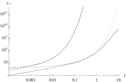
Figure 12: Log-log plot of the growing perturbation mode $x_{+}(\hat{\tau})$ for $\eta=0.1$ (lower curves) and $\eta=0.01$ (upper curves). The solid lines are numerical solutions started up from (134) at small $\tau=0.0001$, the dashed lines are given by the WKB approximation (87) with the exact values of $\Gamma(\hat{\tau})$ and $T(\hat{\tau})$, and the dotted lines are the ultrarelativistic (Bessel function) approximation (134), normalised to agree with the WKB approximation. The power-law growth of both the exact mode and its ultrarelativistic approximation at small $\tau$ visible here is in fact linear, as can be shown from (134). It can be seen that the WKB approximation is good at large $\hat{\tau}$/small $E$, and the ultrelativistic approximation in the other regime. Note that our self-force data are valid only for $\hat{\tau}\gtrsim 0.2$, corresponding to $r>3.02$. It is clear from the figure that starting the numerical integration with data from the ultrarelativistic approximation at $\hat{\tau}=0.2$ instead of $0.001$ would make little difference for $\eta=0.1$ and very little difference for $\eta=0.01$.

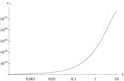
Figure 13: Log-log plot of the growing perturbation mode $x_{+}(\hat{\tau})$ for $\eta=0.01$, showing the full range. The lines are as in Fig. 12. From this and the preceding figure it is clear that the WKB approximation (87) is excellent for $\hat{\tau}\gtrsim 0.2$ for $\eta=0.1$, and $\hat{\tau}\gtrsim 0.001$ for $\eta=0.01$. Continuing this trend, the WKB approximation is good from smaller $\hat{\tau}$ (higher energies) for smaller $\eta$, and it is always good essentially up to plunge.

In numerically evolving $x_{+}$ towards increasing $\hat{\tau}$ from initial data given at small $\tau$ by (134), we stably find the growing WKB solution at large $\tau$. Finding $x_{-}$ over its entire range is more difficult: in going forward from (135), numerical error triggers the growing mode, while going backwards from the WKB form (87) of $x_{-}$ results in a mixture of (134) and (135) as $\hat{\tau}\to 0$. Shooting from both sides would be required, but we have not done this.

References

- (1) V. Cardoso et al., NR/HEP: roadmap for the future, arXiv:1201.5118.
- (2) F. Pretorius and D. Khurana, Black hole mergers and unstable circular orbits, Class. Quant. Grav. 24, S83 (2007).
- (3) K. Martel, Gravitational wave forms from a point particle orbiting a Schwarzschild black hole, Phys. Rev. D 69, 044025 (2004).
- (4) E. Berti et. al., Seminanalytical estimates of scattering thresholds and gravitational radiation in ultrarelativistic black hole encounters, Phys. Rev. D 81, 104048 (2010).
- (5) M. Davis, R. Ruffini, W. H. Press and R. H. Price, Gravitational radiation from a particle falling radially into a schwarzschild black hole, Phys. Rev. Lett. 27, 1466 (1971).
- (6) K. Oohara and T. Nakamura, Gravitational waves from a particle scattered by a schwarzschild black hole. Prog. Theor. Phys. 71, 91 (1984).
- (7) U.Sperhake, V.Cardoso, F.Pretorius, E.Berti, T.Hinderer and N.Yunes, Cross section, final spin and zoom-whirl behaviour in high-energy black hole collisions, Phys. Rev. Lett. 103, 131102 (2009).
- (8) C. Cutler, D. Kennefick and E. Poisson, Gravitational radiation reaction for bound motion around a Schwarzschild black hole, Phys. Rev. D 50, 3816 (1994).
- (9) C. Gundlach and J. M. Martín-García, Critical phenomena in gravitational collapse, Living Reviews in Relativity, 2007-5 (2007), last updated in 2010.
- (10) T. Hinderer and E. E. Flanagan, Two-timescale analysis of extreme mass ratio inspirals in Kerr spacetime: Orbital motion, Phys. Rev. D, 78, 064028 (2009).
- (11) L. Barack and N. Sago, Gravitational self force on a particle in circular orbit around a Schwarzschild black hole, Phys. Rev. D 75, 064021 (2007).
- (12) S. Akcay, A Fast Frequency-Domain Algorithm for Gravitational Self-Force: I. Circular Orbits in Schwarzschild Spacetime, Phys. Rev. D 83, 124026 (2011).
- (13) A. Ori and K. S. Thorne, The Transition from inspiral to plunge for a compact body in a circular equatorial orbit around a massive, spinning black hole, Phys. Rev. D 62, 124022 (2000).
- (14) Ref. Sperhake quotes a maximum fraction of energy radiated of , while its Fig. 2 shows a maximum number of orbits; we have divided the former by the latter. For a boost of , the maximal energy radiated went up to , but the maximal number of orbits is not given.
- (15) M. W. Choptuik and F. Pretorius, Ultra-relativistic particle collisions, Phys. Rev. Lett. 104, 111101 (2010).
- (16) J. Healy, J. Levin and D. Shoemaker, Zoom-whirl orbits in black hole binaries, Phys. Rev. Lett. 103, 131101 (2009).