Divergences and Orientation in Spinfoams

Abstract

We suggest that large radiative corrections appearing in the spinfoam framework might be tied to the implicit sum over orientations. Specifically, we show that in a suitably simplified context the characteristic “spike” divergence of the Ponzano-Regge model disappears when restricting the theory to just one of the two orientations appearing in the asymptotic limit of the vertex amplitude.

I Introduction

Three key open issues in the covariant loop approach to quantum gravity are the presence of two terms of opposite orientation in the asymptotic expansion of the vertex amplitude Barrett:2009mw , the role of gauge-invariance Freidel:2004vi ; Baratin:2011tg ; Bahr:2009mc , and the large-spin divergences. Here we present some indirect evidence that these three issues might be strictly related. While the relation between divergences and gauge has been pointed out Freidel:2002dw ; Baratin:2011tg , the connection with orientation is, as far as we know, new.

In particular, we present some indirect evidence that spinfoam divergences may be generated by the presence of the two terms of opposite orientation in the asymptotic expansion of the vertex amplitude. Pictorially, divergences are generated by geometrical “spikes” where one of the simplices of the spike has orientation opposite to the rest of the geometry. Opposite orientation can be related to time (or parity)-inversion Christodoulou:2012sm in the Lorentzian theory, hence divergences, or, more precisely, large radiative corrections, might come from large fluctuations of the geometry “back and forth in time”.

To illustrate the point, let us start from a puzzle. Let ${}^{4}\tau$ be the triangulation obtained by splitting a single tetrahedron $\tau$ into four tetrahedra via a 1-4 Pachner move, namely by adding a point $P$ connected to all the vertices of $\tau$, as in Figure 1. The Ponzano-Regge amplitude associated to this triangulation is well known to diverge Ponzano:1968uq . This divergence has been associated to the invariance of the amplitude under translations of the point $P$ in the 3d hyperplane defined by the tetrahedron. Indeed, in the asymptotic expansion of the vertex, the amplitude is determined by the Regge action, and the Regge action is invariant under an infinitesimal 3d translation of the point $P$ Morse:1991te . One is therefore led to identify the divergence with the existence of the gauge orbit generated by moving $P$ in the hyperplane defined by $\tau$.

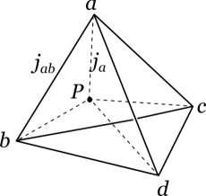
Figure 1: The triangulation ${}^{4}\tau$.

However, the Regge action is invariant in this way only as long as the point $P$ is inside $\tau$. Below we explicitly illustrate this point, perhaps under-appreciated, discussing the geometry of Regge calculus. If the invariance is limited to translations of $P$ within $\tau$, which is compact, how come the amplitude diverges?

We suggest here that the answer lies in the fact that the asymptotic limit of the Ponzano-Regge amplitude is not the exponential of the Regge action, but rather the sum of two exponentials of the Regge action, taken with certain flipped signs. With flipped signs, the invariant contribution comes when $P$ is outside $\tau$. In other words, the divergence is strictly dependent on the existence of the second term in the expansion of the vertex amplitude.

The geometrical origin of this second term can be traced to the fact that the asymptotic limit of the Ponzano-Regge model is not truly 3d general relativity in metric variables, but rather 3d general relativity in triad variables, with an action that flips sign under reversal of the orientation of the triad Rovelli:2012yy . In three dimensions, it is this action (and not metric general relativity) which is equivalent to $BF$ theory. In turn, $BF$ theory has an additional gauge symmetry with respect to general relativity: the shift $B\to B+d_{A}\Phi$ (where $A$ is the connection variable: $F=dA+A\wedge A$), which can be shown to be related to the displacement of $P$ all over the hyperplane Baratin:2011tg .

In this paper, we present two arguments that provide some ground for these intuitions. First, we observe that the only classical solutions of Regge theory on the triangulation ${}^{4}\tau$ are those where $P$ lies inside $\tau$ while in the presence of the flipped-orientation term in the action, there are also classical solutions with $P$ outside $\tau$.

Second, and more specifically, we study in some detail a simplified form of the asymptotic approximation of the sum that defines the divergence. As will be discussed in more detail, the simplifications consist in trivializing the integration measure and in cutting away a region of the integration domain which is more complicated to control since it does not admit a 4d geometrical embedding. Such simplifications define a quantum Regge calculus for the Regge triangulation ${}^{4}\tau$. We show that the corresponding amplitude does not diverge if we take only the Regge term, and diverges if we include the flipped-oriented term.

This is the main technical result of the paper and comes a bit as a surprise, given the intuition that quantum Regge calculus diverges because of the “spikes”. Here we show that crucial spikes at the root of the divergences are those formed by “anti-spacetimes”, in the language of Rovelli:2012yy ; Christodoulou:2012sm . These do not exist in conventional Regge calculus.

The relevance of these observations for the physical four-dimensional quantum gravity is far from granted, but it is suggestive. Looking ahead, we do not think that the moral of our results is that the quantum theory of gravity should be formulated by dropping the flipped term contributions to the dynamics Engle:2011ps ; Engle:2011un ; Engle:2012yg ; Rovelli:2012yy . Rather, it should be better understood what kind of relation exists among “flipped-orientation” (or “anti-spacetime”) quantum fluctuations of the geometry, gauge-invariance, and radiative corrections.

The paper is organized as follows. We start by illustrating the geometry of the spikes in Regge calculus in 2d and in 3d in Section II. In Section III, we discuss the Ponzano-Regge model and its large spin limit, and in Section IV we show how the flipped-orientation terms in the action give rise to new classical solutions, with $P$ outside $\tau$. In Section V, we define the (simplified) integrals corresponding to the amplitudes in a quantum Regge calculus with and without the flipped terms and show that the second amplitude is bounded, while the second is not. Finally we conclude in Section VI.

II Spikes in conventional Regge calculus

We start with an illustration of the geometry of the spikes in 2d and 3d Regge calculus, as this is sometimes a source of confusion. We will deal with spikes which can be embedded in one more dimension (i.e. in 3d and 4d respectively). Remark that this is not the most general possible spike (see Section V for more details).

II.1 Two dimensions

Consider the 2d plane $z=0$ immersed in 3d Euclidean space with coordinates $(x,y,z)$. Consider a triangulation of this plane, containing a triangle $\tau$, whose sides have lengths $j_{ab},\;a,b=1,2,3$. Pick a point $P$ in $\mathbb{R}^{3}$ at a distance $j_{a}$ from the vertices of $\tau$. By joining $P$ with the three vertices of $\tau$, we obtain three triangles $\tau_{a}$, each determined by $P$ and one of the three sides of $\tau$. The 1-3 Pachner move $\tau\to{}^{3}\tau=\{\tau_{a}\}$ modifies the original (flat) triangulation into a triangulation which is in general curved. In particular, there is discrete (distributional) curvature at $P$, given by the deficit angle

$$\delta_{P}:=2\pi-\sum_{a}\theta_{a},$$ (1)

where $\theta_{a}$ is the angle at $P$ of the triangle $\tau_{a}$. The discrete curvature $\delta_{P}$ is a well-defined continuous function of the position of $P$ in $\mathbb{R}^{3}$. It vanishes if $P$ lies in $\tau$ and increases monotonically if $P$ moves perpendicularly away from $\tau$. Therefore if $P$ lies in $\tau$ and we consider infinitesimal shifts in its position, there are two directions that do not change the curvature (see the left side of Figure 2) and one that does.

      

Figure 2: 2d triangulation. Left: $P$ inside $\tau$ and no curvature at $P$. Right: $P$ outside the plane of $\tau$ and curvature at $P$.

Now, what is the value of the curvature if $P$ lies on the plane $z=0$, but outside $\tau$? A moment of reflection shows that in this case the curvature does not vanish. This can be seen for instance rather simply using continuity: consider a situation where the three lengths $j_{a}$ are large compared to the size of $\tau$. Then each of the three angles $\theta_{a}$ is small, and the deficit angle is near $2\pi$. If we move $P$ continuously toward the plane $z=0$ (but still far from $\tau$), the three angles remain small and $\delta_{P}$ remains near $2\pi$. On $z=0$, one of the three angles, say $\theta_{b}$, will become equal to the sum of the other two (see right side of Figure 2), but this does not change the fact that the curvature at $P$ is high.

It is important to observe that the topology of the triangulation is not affected by this degenerate case. The degeneracy is in the embedding of the 2d triangulated surface into $\mathbb{R}^{3}$, not in the topology of the triangulation, which is determined by its intrinsic geometry and which remains $\mathbb{R}^{2}$. Confusing the intrinsic topology of the 2d triangulation with that induced by its embedding in $\mathbb{R}^{3}$ is the source of the misleading intuition that the triangulation with $P$ in the plane but outside $\tau$ is flat.

The only part of the plane where the curvature is constant is the interior of $\tau$.

II.2 Three dimensions

Let us repeat now the same construction in 3d. Consider a tetrahedron $\tau$ lying in the 3d hyperplane $s=0$ immersed in 4d Euclidean space with coordinates $(x,y,z,s)$, with sides having lengths $j_{ab},\;a,b=1,2,3,4$. Pick a point $P$ in $\mathbb{R}^{4}$ and let $j_{a}$ be the distances of $P$ from the vertices of $\tau$. By joining $P$ with the four vertices of $\tau$, we obtain four tetrahedra $\tau_{a}$, each determined by $P$ and one of the four triangles which bound $\tau$. The 1-4 Pachner move $\tau\to{}^{4}\tau=\{\tau_{a}\}$ splits the original tetrahedron into a triangulation (Figure 1) which is generally curved. In particular, there is distributional curvature $\theta_{a}$ at each of the four segments joining $P$ with the vertices of $\tau$, given by the deficit angles

$$\delta_{a}:=2\pi-\sum_{b\neq a}\theta_{a}^{b},$$ (3)

where $\theta_{a}^{b}$ is the internal dihedral angle at the edge $a$ of the tetrahedron $\tau_{b}$ (Figure 3).

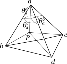
Figure 3: Absence of curvature in 3d triangulation with $P$ inside $\tau$.

Again, the deficit angle is a well-defined continuous function of the position of $P$ in $\mathbb{R}^{4}$. It vanishes if $P$ lies in $\tau$ (Figure 3) and becomes non zero when $P$ is taken perpendicularly away from $\tau$ in $\mathbb{R}^{4}$ (Figure 4). Therefore if $P$ lies in $\tau$ and we consider infinitesimal shifts in its position, there are three directions that do not change the curvature, and one that does.

Now, what is the value of the curvature if $P$ lies in the hyperplane $s=0$, but outside $\tau$? As before, in this case the curvature does not vanish. As in the two dimensional case, this can be shown by continuity. However the argument is more subtle, since the dihedral angles do not necessarily go to zero as $P$ goes to infinity; nevertheless, as it will be shown in section V, in this limit the sum of the three dihedral angles associated to the edges $(bP),(cP)$ and $(dP)$ of the tetrahedron $\tau_{a}$ goes to $\pi$; thus, the sum of all twelve such dihedral angles is $4\pi$, and not $4\times 2\pi$ (a full turn for each internal edge of the triangulation) as one would expect for the flat case. Therefore, this configuration represents necessarily a curved Regge geometry. If we now move continuously $P$ into the plane $s=0$, the previous argument continues to hold. When $s=0$, one of the three dihedral angles becomes equal to the sum of the other two dihedral angles relative to the same edge (see Figure 4); nevertheless, this does not change the fact that the curvature is non-zero.

As before, the topology of the triangulation is not affected by this degenerate case: the degeneracy is in the embedding of the 3d triangulated surface into $\mathbb{R}^{4}$, not in the topology of the triangulation, which remains $\mathbb{R}^{3}$.

The only part of the hyperplane where the curvature remains constant and vanishes is the interior of $\tau$.

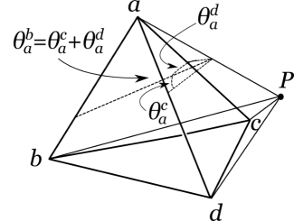
Figure 4: Curvature in 3d triangulation with $P$ outside $\tau$.

III The Ponzano-Regge amplitude in the spin basis

Let us now come to the Ponzano-Regge amplitude. For a given triangulation formed by tetrahedra $v$, triangles $e$ and edges $f$, this is given in the spin basis by Ponzano:1968uq ; Barrett:2008wh

$$W(j_{l}):=\sum_{j_{f}}{}^{\prime}\prod_{f} (-1)^{2j_{f}}(2j_{f}+1)\times$$

$$\times\prod_{e}(-1)^{j_{e_{1}}+j_{e_{2}}+j_{e_{3}}}\prod_{v}\{6j\}_{v}.$$ (5)

Here $j_{f}\,$ are the spins associated to (any of) the edges of a given triangulation, $j_{l}$ are those associated uniquely to its boundary edges, $\{6j\}_{v}$ is the Wigner 6-$j$ symbol associated to the tetrahedron $v$, and $e_{i}$ are the three sides of the triangle $e$. The primed sum runs over the bulk spins alone.

The sign factors are necessary for the topological invariance of the theory as well as for the recovery of general relativity in the continuous limit (see Barrett:2008wh ), and will play a key role below.

For the triangulation ${}^{4}\tau$, the Ponzano-Regge amplitude reads:

$$W(j_{ab})=N(j_{ab})\sum_{j_{a}}\prod_{a}(-1)^{j_{a}}(2j_{a}+1)\prod_{a}\left\{\begin{tabular}[]{@{} ccc @{}}$j_{b}$&$j_{c}$&$j_{d}$\\ $j_{cd}$&$j_{db}$&$j_{bc}$\end{tabular}\right\},$$ (6)

where $N(j_{ab}):=\prod_{(ab)}(-1)^{j_{ab}}(2j_{ab}+1)$ depends only on the boundary edges. In writing this expression we used the fact that $2j_{a}\in\mathbb{N}$, as well as the convention according to which different indices take different values (convention that will be used throughout the whole article). It is well known since the work of Ponzano and Regge that this sum diverges. This can be seen by Fourier transforming from the spins to $SU(2)$ group variables (see Rovelli:2011eq ), which gives

$$W\sim\int_{SU(2)^{4}}dh_{ab}\prod_{a}\delta_{SU(2)}(h_{bc}h_{cd}h_{db})\sim\delta_{SU(2)}(1).$$ (7)

This divergence goes like $j^{3}$, suggesting that it is related to a 3d volume divergence. It is tempting to relate it to the invariance of the Regge amplitude under shifts of the point $P$ in the 3d hyperplane of the tetrahedron $\tau$. Indeed, the divergence comes obviously from the large $j_{a}$’s region, where we can use the asymptotic value for the Wigner 6-$j$ symbols:

$$\{6j\}\sim\frac{1}{\sqrt{3\pi V}}\cos\left(\sum_{f}\Theta_{f}j_{f}+\frac{\pi}{4}\right),$$ (8)

where $\Theta_{f}$ is the external dihedral angle at the edge $f$ of a tetrahedron having sides with lengths $j_{f}$, and $V$ is the volume of this tetrahedron. Remarkably, if the six $j_{f}$’s are such that they do not close geometrically into triangles, then the corresponding 6-$j$ symbol is ill-posed and set to zero; moreover, if they do geometrically close into triangles, but they do not into a tetrahedron, then the corresponding 6-$j$ symbol in the large $j$ limit is exponentially suppressed.

Inspired by this asymptotic behaviour, in a notation suitable for ${}^{4}\tau$, we define

$$A_{\pm}^{a}=\frac{1}{\sqrt{12\pi V_{a}}}\exp\left[{\pm i\left(\sum_{\varepsilon\subset\tau_{a}}\Theta_{\varepsilon}^{a}j_{\varepsilon}+\frac{\pi}{4}\right)}\right],$$ (9)

where $V_{a}$ is the volume of the tetrahedron $\tau_{a}$, and where the sum runs over its edges. Then, the asymptotic limit of (6) can be split into sixteen terms

$$W(j_{ab}) \sim N(j_{ab})\sum_{j_{a}}\prod_{a}(-1)^{j_{a}}(2j_{a}+1)\prod_{a}(A^{a}_{+}+A^{a}_{-})$$ (10)

$$\sim \ \ \sum_{\pm\pm\pm\pm}W_{\pm\pm\pm\pm}(j_{ab}).$$

The analysis of these terms will be the central topic of the next section.

IV The $W_{\pm\pm\pm\pm}$’s and their saddle points

In this section we give an expression of the $W_{\pm\pm\pm\pm}$ for each of the four relevant combinations of $\pm$ signs, we discuss the continuum (large $j$) limit and the relation of the latter to the classical equation of motion.

Using the definition given implicitly through equation (10) and by writing the $(-1)^{j}$ factors as $e^{ik\pi j}$, $k\in(2\mathbb{Z}+1)$, (more will be said about this ambiguity later) one finds

$$W_{\pm\pm\pm\pm} =N^{\prime}(j_{ab})\sum_{j_{a}}\mu[j_{f}]e^{i\sum_{(ab)}j_{ab}\left[\pm_{c}\Theta_{ab}^{c}\pm_{d}\Theta_{ab}^{d}+k\pi\right]}\times$$

$$\qquad\qquad\qquad\times e^{i\sum_{a}j_{a}\left[\pm_{b}\Theta^{b}_{a}\pm_{c}\Theta^{c}_{a}\pm_{d}\Theta^{d}_{a}+k\pi\right]}$$

$$=:N^{\prime}(j_{ab})\sum_{j_{a}}\mu[j_{f}]e^{iS_{\pm\pm\pm\pm}}\;,$$ (11)

where $N^{\prime}(j_{ab}):=\prod_{(ab)}(2j_{ab}+1)$, $\mu[j_{f}]:=\prod_{a}\frac{2j_{a}+1}{\sqrt{12\pi V_{a}}}$, and $\pm_{a}$ is plus or minus according to which one between $A_{+}^{a}$ and $A_{-}^{a}$ appears in $W_{\pm\pm\pm\pm}$. Finally in (11) we defined an “action” $S_{\pm\pm\pm\pm}$ for each $W_{\pm\pm\pm\pm}$. We can now switch from external ($\Theta$) to internal dihedral angles ($\theta$) by using the relation: $\Theta=\pi-\theta$. This straightforwardly leads to:

$$S_{++++}= \sum_{(ab)}j_{ab}\left[(2+k)\pi-\theta_{ab}^{c}-\theta_{ab}^{d}\right]+$$

$$+\sum_{a}j_{a}\left[(3+k)\pi-(\theta^{b}_{a}+\theta^{c}_{a}+\theta^{d}_{a})\right],$$ (12)

$$S_{+++-}= \dots+\sum_{a\neq 4}j_{a}\left[(1+k)\pi-(\theta^{b}_{a}+\theta^{c}_{a}-\theta^{4}_{a})\right]+$$

$$+j_{4}\left[(3+k)\pi-(\theta^{1}_{4}+\theta^{2}_{4}+\theta^{3}_{4})\right],$$ (13)

$$S_{++--}= \dots+\sum_{a=1,2}j_{a}\left[(-1+k)\pi-(\theta^{b}_{a}-\theta^{3}_{a}-\theta^{4}_{a})\right]+$$

$$+\sum_{c=3,4}j_{c}\left[(1+k)\pi-(\theta^{1}_{c}+\theta^{2}_{c}-\theta^{d}_{c})\right],$$ (14)

$$S_{+---}= \dots+j_{1}\left[(-3+k)\pi+\theta^{2}_{1}+\theta^{3}_{1}+\theta^{4}_{1}\right]+$$

$$+\sum_{a\neq 1}j_{a}\left[(-1+k)\pi-(\theta^{1}_{a}-\theta^{b}_{a}-\theta^{c}_{a})\right],$$ (15)

$$S_{----}= \sum_{(ab)}j_{ab}\left[(-2+k)\pi+\theta_{ab}^{c}+\theta_{ab}^{d}\right]+$$

$$+\sum_{a}j_{a}\left[(-3+k)\pi+\theta^{b}_{a}+\theta^{c}_{a}+\theta^{d}_{a}\right].$$ (16)

In (13-15) dots indicate that we omitted the terms associated to the boundary spins, which are however irrelevant for the following.

Now, we come to the specific choice of $k\in(2\mathbb{Z}+1)$. This choice is imposed by the fact that we want to recover the Regge action in the large-$j$ continuum limit. We see that only (12) and (16) are good (mutually exclusive) candidates for this. In fact they are the only actions which contain for every internal edge the sum of all the three associated dihedral angles which appears in the definition of the deficit angle. Therefore, if we want to make $S_{+}:=S_{++++}$ essentially equal to the Regge action $S_{R}=\sum_{f}j_{f}\delta_{f}$ we have to choose $k=-1$; conversely if we want to make $S_{-}:=S_{----}$ essentially equal to (minus) the Regge action, we have to choose $k=1$.

The two choices are symmetric, i.e. relate $S_{\pm\pm\pm\pm}$ in one case to $-S_{\mp\mp\mp\mp}$ in the other. Choose once and for all

$$k=-1,\text{ so that }S_{+}\sim S_{R}.$$ (17)

Notice that once this choice is done, no symmetry is any more present among the previous actions (12-16). This fact entails an important consequence, which is important for the coherence of our results in section V: i.e. only the actions $S_{+}$ and $S_{+++-}$ have a (large set) of classical solutions. In the following of this section we shall justify and discuss this statement.

As it is customary, we define the classical solutions to be described by the stationary points of the action, picked out by letting $j_{a}$’s go to infinity. Hence, the classical equations of motion for (12-16) are respectively:

$$S_{+}\sim S_{R}\; :\;\delta_{a}:=2\pi-(\theta_{a}^{b}+\theta_{a}^{c}+\theta_{a}^{d})=0;$$ (18)

$$S_{+++-}\; :\;\left\{\begin{array}[]{ll}\theta_{a}^{b}+\theta_{a}^{c}=\theta_{a}^{4},&a\neq 4\\ \delta_{4}=0\end{array}\right.;$$ (21)

$$S_{++--}\; :\;\left\{\begin{array}[]{ll}\theta_{a}^{3}+\theta_{a}^{4}=\theta_{a}^{b}+2\pi,&a=1,2\\ \theta^{1}_{c}+\theta^{2}_{c}=\theta^{d}_{c}&c=3,4\end{array}\right.;$$ (24)

$$S_{+---}\; :\;\left\{\begin{array}[]{ll}\theta_{1}^{2}+\theta_{1}^{3}+\theta_{1}^{4}=4\pi\\ \theta^{b}_{a}+\theta^{c}_{a}=\theta^{1}_{a}+2\pi\end{array}\right.;$$ (27)

$$S_{-}\; :\;\theta_{a}^{b}+\theta_{a}^{c}+\theta_{a}^{d}=4\pi.$$ (28)

As it is well known, Equation (18) is the flatness condition expressed in the language of Regge geometry, i.e. by the vanishing of all deficit angles; solutions to these equations are the quadruplets of lengths $j_{a}$ given by the distances between the vertices of $\tau$ and a point $P$ situated anywhere inside $\tau$ (see Section II).

Solutions to Equation (21) are similarly parametrized by the position of the point $P$ in a specific region of $\mathbb{R}^{3}$, via an embedding of the triangulation. In this case, however, such a region, say $\mathcal{R}_{4}$, is non-compact and lies outside the tetrahedron $\tau$. $\mathcal{R}_{4}$ is the disconnected union of two regions, $\mathcal{R}_{4}^{f}$ and $\mathcal{R}_{4}^{v}$; loosely speaking $\mathcal{R}_{4}^{f}$ correspond to the sector of $\mathbb{R}^{3}$ from which one cannot “see” the fourth vertex of $\tau$, since it is “hidden” by the tetrahedron $\tau$ itself (see Figure 4), while $\mathcal{R}_{4}^{v}$ is the point reflected of $\tau\cup\mathcal{R}_{4}^{f}$ with respect to the fourth vertex of $\tau$.

The saddle point equations (24) for $S_{++--}$ are slightly more involved. First, recall that $0\leq\theta_{a}^{b}\leq\pi$, then by the first pair of equations one gets $\theta_{2}^{c}=\theta_{1}^{c}=\pi$; this is possible only if $P$ lies on the face $(12d)$, with $d\notin\{1,2,c\}$ of $\tau$; since $d\in\{3,4\}$, this means that $P$ lies on the edge $(12)$; the second pair of equations in (24) has the same solution, in fact it is satisfied only if $P$ lies at the same time in $\mathcal{R}_{3}$ and $\mathcal{R}_{4}$, i.e. if $P$ lies on the edge $(12)$. Thus, the classical solutions to the action $S_{++--}$ are parametrized by $P\in(12)$.

Finally, Equations (27) and (28) have no classical solution. To see this, just recall once more that $0\leq\theta_{a}^{b}\leq\pi$, and remark that therefore $\theta_{a}^{b}+\theta_{a}^{c}+\theta_{a}^{d}\leq 3\pi<4\pi$.

Thus, we showed that the classical solutions to the asymptotic $j\gg 1$ Ponzano-Regge model come mainly from two different sectors of the asymptotic limit (in fact the solutions stemming from $S_{++--}$ are given by a compact region of co-dimension three with respect to the phase space $\{j_{a}\}$; therefore, they are practically irrelevant for any concrete purpose). Moreover the solutions stemming from the $S_{+}\sim S_{R}$ sector are all gauge equivalent since they describe the very same geometry. However, the corresponding gauge orbit is compact, and for this reason it is hard to explain the model’s divergences by saying that they arise from the integration over such gauge equivalent solutions. On the other hand, there exist four infinite non-compact sets of classical solutions which have co-dimension one, stemming from the terms of the type $S_{+++-}$. It is then quite tempting to associate the divergence of the Ponzano-Regge amplitude of ${}^{4}\tau$ to the existence of this three dimensional hyper-surfaces of saddle points (recall that $W[^{4}\tau]$ diverges like $j^{3}$).

In the following section, we explore this hypothesis from quite a different point of view, by studying explicitly (even if under some simplifying assumptions) a certain continuum version of the $W_{\pm\pm\pm\pm}$.

V Boundedness of the Regge spike

We now come to the main technical result of this paper. We study a continuum and simplified version of the amplitude $W_{+}$ and we show that it is bounded. The argument then fails for the corresponding integral in the $W_{+++-}$ case (but stays valid in the remaining cases).

We first rewrite $W_{+}$ in the limit where the $j$’s become continuum variables, dubbed $l_{a}$ and $l_{ab}$, in the case of bulk and boundary edge lengths respectively:

$$W_{+}(l_{ab})\approx N^{\prime}(l_{ab})\int_{\Omega}d\mu[l_{a}] e^{i\sum_{(ab)}l_{ab}\left[\pi-\left(\theta_{ab}^{c}+\theta_{ab}^{d}\right)\right]}\times$$

$$\times e^{i\sum_{a}l_{a}\left[2\pi-\left(\theta_{a}^{b}+\theta_{a}^{c}+\theta_{a}^{d}\right)\right]},$$ (29)

where the domain of integration $\Omega$ is given by the quadruplets of lengths that satisfy two sets of conditions, which assure from the algebraic point of view that the 6-$j$ symbols are well defined and from the geometrical point of view that the corresponding segments close into triangles and tetrahedra following the combinatorics of the triangulation ${}^{4}\tau$. Remark that no condition is required for all of them to close at the same time, neither in $\mathbb{R}^{3}$ nor in $\mathbb{R}^{4}$.

The simplification we consider is first to replace the non-trivial measure factor $d\mu[l_{a}]$ with a simple Lebesgue measure $d^{4}l_{a}$. Second, to restrict the integration domain $\Omega$ to the set $\omega$ of the quadruplets $l_{a}$ given by the distances from a point $P$ in $\mathbb{R}^{4}$. This is a restriction because a priori, as we stressed in the previous paragraph, the $j_{a}$’s (and therefore the $l_{a}$’s) can define a Regge 3d geometry that cannot be embedded in $\mathbb{R}^{4}$. Therefore $\omega$ is smaller than $\Omega$.

Hence, we define the following integral, which will be the starting point for the rest of our considerations

$$I_{+}(l_{ab}):=\int_{\omega}d^{4}l_{a}e^{i\sum_{(ab)}l_{ab}\delta_{ab}+i\sum_{a}l_{a}\delta_{a}},$$ (30)

where

$$\left\{\begin{array}[]{rl}\delta_{ab}:=&\pi-\left(\theta_{ab}^{c}+\theta_{ab}^{d}\right)\\ \delta_{a}:=&2\pi-\left(\theta_{a}^{b}+\theta_{a}^{c}+\theta_{a}^{d}\right)\end{array}\right.$$ (31)

are the boundary and bulk deficit angles, respectively.

Switching integration variables from edge lengths $\{l_{a}\}$, to the 4d coordinates of the point $P$, say $\{x^{P}_{i}\}_{i=1,\dots,4}$, and then to spherical coordinates in $\mathbb{R}^{4}$, that is $\{\rho_{P},\alpha^{P}_{l}\}_{l=1,\dots,3}$; omitting the label $P$, this yields

$$\left\{\begin{array}[]{c c l}x_{1}&=&\rho\sin\alpha_{2}\sin\alpha_{2}\sin\alpha_{1}\\ x_{2}&=&\rho\sin\alpha_{3}\sin\alpha_{2}\cos\alpha_{1}\\ x_{3}&=&\rho\sin\alpha_{3}\cos\alpha_{2}\\ x_{4}&=&\rho\cos\alpha_{3}.\end{array}\right.$$ (36)

Under this change of variables the integration measure changes in the following way:

$$d^{4}l_{a}=\left\|\frac{\partial l_{a}}{\partial x_{i}}\right\|\left\|\frac{\partial x_{i}}{\partial(\rho,\alpha_{l})}\right\|d\rho d^{3}\alpha_{l}\approx f(\alpha_{l})d\rho d^{3}\alpha_{l}.$$ (37)

Here, $f(\alpha_{l})$ is a function (that we do not need to give explicitly for our purposes) of the angular variables of $S^{3}$ only, whose typical length scale is given by the size of the boundary tetrahedron. In these variables, the integral (30) takes the form

$$I_{+}(l_{ab})\approx \int_{0}^{\infty}d\rho\int_{S^{3}}d^{3}\alpha_{l}\;f(\alpha_{l})e^{i\sum_{(ab)}l_{ab}\delta_{ab}+i\sum_{a}l_{a}\delta_{a}},$$ (38)

where now all edge lengths and dihedral angles are considered as functions of $\rho$ and $\alpha_{l}$. Next, we consider the large $\rho$ asymptotics of the argument of the exponent of (38). The asymptotic form can be best understood by drawing a tetrahedron, adding a fifth vertex $P$ in $\mathbb{R}^{4}$ and pulling it to infinity (Figure 5).

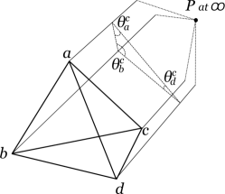
Figure 5: A tetrahedron with an additional fifth vertex at infinity. One can see that the sum of the internal dihedral angles of the same tetrahedron (labelled tetrahedron $c$ above) becomes $\pi$. The same is obviously true for the dihedral angles of the other three tetrahedra.

We can immediately see that the 4-simplex obtained in this way looks in first approximation as a 4 dimensional prism, with a tetrahedron as its basis. Clearly, the same statement, just transposed into one less dimension, holds also for all the tetrahedra formed by the point $P$ and one of the faces of the original tetrahedron. In such a configuration the sum of the internal dihedral angles belonging to one of these ”stretched out” tetrahedra will go to $\pi$ when $P$ approaches infinity:

$$\text{in $\tau_{a}$: }\sum_{b\neq a}\theta_{b}^{a}\xrightarrow{P\rightarrow\infty}\pi.$$ (39)

Moreover, if $P$ approaches infinity at angles $\alpha_{l}$ fixed and $\rho\rightarrow\infty$, it is clear that all four edge lengths scale as $l_{a}=\rho+\text{const.}+\mathcal{O}(\rho^{-1})$. Hence, taking into account all the four tetrahedra, we can easily deduce that our integral takes the following asymptotic form

$$I_{+}(l_{ab})\approx \int_{0}^{\infty}d\rho\int_{S^{3}}d^{3}\alpha_{l}\;f(\alpha_{l})\exp\Big{[}i\large(4\pi\rho+F(\alpha_{l})$$

$$+G(\alpha_{l},\rho)\large)\Big{]}.$$ (40)

Here, $F(\alpha_{l})$ is solely a function of the angles and $G(\alpha_{l},\rho)$ is the remaining part of the action which goes monotonically to 0 when $\rho$ goes to infinity at fixed $\mathbf{\alpha}$; notice that $G$ does not contain any higher orders of $\rho$ than $\rho^{-1}$. For this expansion to be useful, we must have that $\rho\gg\max\{l_{ab}\}$, where $l_{ab}$ are the edge length of the fixed (boundary) tetrahedron. In this case, the expansion of the integrand in (38) follows directly from the definitions of the dihedral angles in our choice of variables. The integral (40) is bounded thanks to the oscillations provided by the $4\pi\rho$ term. This fact is shown in detail in Appendix A. The result to be kept in mind is that the previous integral is bounded independently on the size of the Regge spike in $\mathbb{R}^{4}$.

Next, we move on to consider the integral $I_{+++-}(l_{ab})$, corresponding to $W_{+++-}$. In this case the integral reads

$$I_{+++-}(l_{ab}):= \int_{\omega}d^{4}l_{a}\;\exp\Big{[}\dots+ij_{4}\delta_{4}+$$

$$+\sum_{a\neq 4}j_{a}\left(\theta^{4}_{a}-\theta^{b}_{a}-\theta^{c}_{a}\right)\Big{]},$$ (41)

where the dots stand for the boundary edge terms, whose details are unessential for our analysis. Manipulating this integral in the same way we did for $I_{+}$, i.e. going to $\mathbb{R}^{4}$ spherical variables and taking the $\rho\rightarrow\infty$ limit, it is easy to show that in the action the leading order term in $\rho$ vanishes. Actually, the absence of the leading term in $\rho$ is a peculiarity of the $I_{+++-}$ integral (41); indeed, it does not happen for the $I_{++--},\;I_{+---}$ or $I_{-}$ cases. In each of them the leading term is $-4\pi\rho,-8\pi\rho$ and $-12\pi\rho$ respectively, and the corresponding integrals are bounded, for the very same reason that $I_{+}$ is. This mirrors our geometrical analysis of the saddle points of the $W_{\pm\pm\pm\pm}$ carried out in Section IV.

Accordingly (41) takes the following asymptotic form:

$$I_{+++-}(l_{ab})\approx \int_{0}^{\infty}d\rho\int_{S^{3}}d^{3}\alpha_{l}\;f(\alpha_{l})\exp\Big{[}i\large(F_{-}(\alpha_{l})+$$

$$+G_{-}(\alpha_{l},\rho)\large)\Big{]}.$$ (42)

Here, as in the $I_{+}(l_{ab})$ case, the function $F_{-}(\alpha_{l})$ is only a function of the $S^{3}$ angles and $G_{-}(\alpha_{l},\rho)$ is a function that goes monotonically to 0 as $\rho\rightarrow\infty$. By our choice of the measure $d\mu[l_{a}]\to d^{4}l_{a}$, any possible divergence arising in this integral comes from very large $\rho$’s; therefore in looking for divergences we can expand the integrand for $\rho\gg l_{ab}$; in doing this, we get

$$f(\alpha_{l})e^{iF_{-}(\alpha_{l})}\Big{[}1+iG_{-}(\alpha_{l},\rho)+\mathcal{O}(\rho^{-2})\Big{]}.$$ (43)

The above integrand clearly has a linear and a logarithmic divergence when integrated over $\rho$ up to infinity, which are given by its first two terms respectively, while its remainder is convergent. Therefore, the integral $I_{+++-}(l_{ab})$ is in fact divergent, as a consequence of the sign flip.

VI Summary and Outlook

We have pointed out that if we consider the triangulation ${}^{4}\tau$ obtained by adding a point $P$ to a tetrahedron $\tau$, as a Regge geometry, the only flat configurations are those where $P$ is inside the boundary of the tetrahedron $\tau$; these flat solutions are all gauge equivalent. Any other configuration of ${}^{4}\tau$, where the point $P$ is outside $\tau$, is not flat and carries curvature, depending on the position of the point $P$.

The Ponzano-Regge amplitude of the triangulation defined by ${}^{4}\tau$ is well-known to diverge. In the spin representation such divergence scales like $j^{3}$ in the cut-off spin. We have analysed the Ponzano-Regge model in its large $j$ limit, where the 6-$j$ symbol is known to behave like the cosine of the Regge action (plus a phase irrelevant here) multiplied by some (crucial) signs. Since ${}^{4}\tau$ is composed by four tetrahedra $\tau_{a}$, the full amplitude is given by the sum of 16 terms. Each of these can be approximated by a path integral whose action $S_{\pm\pm\pm\pm}$ is - loosely speaking - given by the sum of plus or minus the Regge action for each of the four $\tau_{a}$’s. We analysed the classical equation of motion (i.e. the saddle points of the path integral at large $j$’s) for each $S_{\pm\pm\pm\pm}$ and found that there are two main classes of solutions, where the point $P$ lies respectively inside or outside $\tau$. In the first case these are solutions of the $S_{++++}\sim S_{\rm Regge}[^{4}\tau]$ action, and are flat and gauge equivalent (in the Regge geometry sense); they form a compact set in the space of the edge-lengths. In contrast, if $P$ lies outside $\tau$, these are solutions of one of the $(S_{+++-})$-like actions and encode a set of curved, non-gauge-equivalent Regge geometries; they form a non-compact set in the space of the edge-lengths. Having found two sets of saddle points for the Ponzano-Regge amplitude of ${}^{4}\tau$, we then wanted to explicitly evaluate the path integral of its different terms, to see which ones are at the origin of the divergence and to check if there was any correlation between their divergences and their sets of saddle points.

To be able to evaluate these integrals we had to considerably simplify them. The simplifications consist in trivializing the path integral measure $d\mu[l_{a}]=\left[\prod_{a}\frac{2l_{a}+1}{(12\pi V_{a})^{1/2}}\right]d^{4}l_{a}\to d^{4}l_{a}$, as well as in restricting the integration domain to those edge lengths which have an embedding in $\mathbb{R}^{4}$.

We hence showed that the only divergent path integral is the one related to the $(S_{+++-})$-like actions. Its divergence is linear in the edge-length scale, and not cubic. The discrepancy with the Ponzano-Regge result can be traced to the use of a different measure. In fact each of the $(2l_{a}+1)$ factors would take into another $l$ factor, while each volume another $l^{-1/2}$ factor. The total degree of divergence would hence be $1+4\times 1+4\times(-\frac{1}{2})=3$. Unluckily, restoring the original measure entails many complications, which could eventually spoil our result. Despite of this, we think that this calculation can teach us something about the divergences: in fact it shows explicitly, even if in the context of a slightly artificial variation of the Ponzano-Regge model, how the presence of the two signs in the asymptotics can be (one of the) sources of divergences in the large $j$ regime.

These observations are relevant because several spinfoam theories, and in particular Lorentzian loop quantum gravity in four dimensions Rovelli:2011eq , contain the same two terms in the asymptotic expansion of the vertex. This work is in a context of general effort to understand the possible implications of the presence of these two terms. For a recent discussion on the physics of the terms, see Christodoulou:2012sm . In the language of that paper and Rovelli:2012yy , divergences appear to be generated by “antispacetime” fluctuations of the geometry, or fluctuations of the geometry “back and forth in time”.

—

Appendix A Boundedness of $I_{+}(l_{ab})$

In this appendix we show that the integral $I_{+}(l_{ab})$ defined in Equation (30) is bounded in an appropriate sense to be specified below.

We first define a cut-off version of the integral $I_{+}(l_{ab})$:

$$I_{+}^{C}(l_{ab})= \int_{0}^{C}d\rho\int_{S^{3}}d^{3}\alpha_{l}\;f(\alpha_{l})\exp\left[i\sum_{bc}l_{bc}(\theta^{a}_{bc}+\theta^{d}_{bc})\right.$$

$$\left.+i\sum_{b}l_{b}(2\pi-(\theta^{a}_{b}+\theta^{c}_{b}+\theta^{c}_{b}))\right].$$ (44)

Then we show that $I_{+}^{C}(l_{ab})$ is bounded by a number independent of the cut-off $C$. As it will be clear soon, we cannot just say that the whole integral $I_{+}$ converges because its value is not defined, since it contains an ever-oscillating contribution. To show our claim, we begin with the form (40) of the integral $I^{C}_{+}(l_{ab})$, and we do the following manipulations to it:

$$I_{+}^{C}= \int_{0}^{C}d\rho\int_{S^{3}}d^{3}\alpha_{l}\;f(\alpha_{l})\exp\Big{[}i(4\pi\rho+F(\alpha_{l})+$$

$$+G(\alpha_{l},\rho))\Big{]}$$ (45)

$$= \;\int_{S^{3}}d\mu[\alpha_{l}]\int_{0}^{C}d\rho\;\exp\Big{[}4\pi i\rho+iG(\alpha_{l},\rho)\Big{]}$$ (46)

$$= \;\int_{S^{3}}d\mu[\alpha_{l}]\int_{0}^{C}d\rho\;\Big{\{}\exp({4\pi i\rho})+$$

$$+\exp({4\pi i\rho})\big{[}\cos(G(\alpha_{l},\rho))-1+i\sin(G(\alpha_{l},\rho))\big{]}\Big{\}}$$ (47)

$$= \;\mathcal{F}e^{4\pi iC}+\int_{S^{3}}d\mu[\alpha_{l}]\int_{0}^{C}d\rho\;\Big{\{}\exp({4\pi i\rho})\times$$

$$\times\big{[}\cos(G(\alpha_{l},\rho))-1+i\sin(G(\alpha_{l},\rho))\big{]}\Big{\}}.$$ (48)

In equation (46), we changed the order of integration and defined $d\mu[\alpha_{l}]:=f(\alpha_{l})\exp[iF(\alpha_{l})]d^{3}\alpha_{l}$; while in (48) we defined $\mathcal{F}:=(4\pi i)^{-1}\int_{S^{3}}d\mu[\alpha_{l}]$.
Let us now consider the remaining integral in (48). To start, we focus on the integration over $\rho$ at fixed $\alpha_{l}$’s:

$$A^{C}(\alpha_{l})=\int_{0}^{C}d\rho\;e^{4\pi i\rho}\big{[}\cos(G(\alpha_{l},\rho))-1+i\sin(G(\alpha_{l},\rho))\big{]}.$$ (49)

We split $A^{C}$ in real and imaginary part. Each of these is composed of two terms, in which an oscillating function ($\sin(4\pi\rho)$ or $\cos(4\pi\rho)$) multiplies either $\sin(G)$ or $[\cos(G)-1]$. The latter two functions approach monotonically zero for $\rho$ larger than a certain value (which depends on the $\alpha_{l}$’s), just by the fact that $G$ is an analytic function of $\rho$ whose limit is zero when $\rho$ goes to infinity. By Dirichlet’s test (see Appendix B for a reminder) it is immediate to see that each of these terms converge for any $\alpha_{l}$’s when $C$ goes to infinity. So $A(\alpha_{l})=\lim_{C\rightarrow\infty}A^{C}(\alpha_{l})$ are complex numbers of finite norm.
Hence:

$$\lim_{C\rightarrow\infty} \Big{[}I_{+}^{C}-\mathcal{F}e^{4\pi iC}\Big{]}=\lim_{C\rightarrow\infty}\int_{S^{3}}d^{3}\mu[\alpha_{l}]\;A^{C}(\alpha_{l})$$

$$=\int_{S^{3}}d^{3}\alpha_{l}\;f(\alpha_{l})\exp[iF(\alpha_{L})]A(\alpha_{l})$$ (50)

which is finite in norm and well-defined, since we are integrating a regular function over a compact domain.
This means that the original integral $I_{+}(l_{a})$, even if not well-defined as a complex number, is still uniformly bounded for any value of the cut-off $C$, i.e. for any size of the spike.

Appendix B Dirichlet’s Test

Dirichlet’s test for the convergence of integrals goes as follows.
If two functions $f(x)$ and $g(x)$ are such that

$$\left|\int_{a}^{y}dx\;f(x)\right|<M,\;\forall y>a$$ (51)

for a certain real fixed $M$, and

$$g(x)\xrightarrow{x\rightarrow\infty}0\;\text{monotonically for }x>a,$$ (52)

then the integral of their product converges:

$$\left|\int_{a}^{\infty}dx\;f(x)g(x)\right|<\infty.$$ (53)

References

C. Rovelli, “Zakopane lectures on loop gravity,” arXiv:1102.3660.

J. W. Barrett, R. Dowdall, W. J. Fairbairn, F. Hellmann, and R. Pereira, “Lorentzian spin foam amplitudes: Graphical calculus and asymptotics,” Class.Quant.Grav. 27 (2010) 165009, arXiv:0907.2440.

L. Freidel and D. Louapre, “Ponzano–Regge model revisited. I: Gauge fixing, observables and interacting spinning particles,” Class. Quantum Grav. 21 (2004) 5685.

A. Baratin, F. Girelli, and D. Oriti, “Diffeomorphisms in group field theories,” arXiv:1101.0590.

B. Bahr and B. Dittrich, “Breaking and restoring of diffeomorphism symmetry in discrete gravity,” arXiv:0909.5688.

W. J. Fairbairn and C. Meusburger, “Quantum deformation of two four-dimensional spin foam models,” arXiv:1012.4784.

M. Han, “Cosmological Constant in LQG Vertex Amplitude,” arXiv:1105.2212.

C. Rovelli, “On the structure of a background independent quantum theory: Hamilton function, transition amplitudes, classical limit and continuous limit,” arXiv:1108.0832.

L. Freidel and D. Louapre, “Diffeomorphisms and spin foam models,” Nucl. Phys. B662 (2003) 279–298, arXiv:gr-qc/0212001.

M. Christodoulou, A. Riello, and C. Rovelli, “How to detect an anti-spacetime,” arXiv:1206.3903.

G. Ponzano and T. Regge, “Semiclassical limit of Racah coefficients,” in Spectroscopy and group theoretical methods in Physics, F. Bloch, ed. North-Holland, Amsterdam, 1968.

P. A. Morse, “Approximate diffeomorphism invariance in near flat simplicial geometries,”. UCSBTH-91-46.

C. Rovelli and E. Wilson-Ewing, “Discrete Symmetries in Covariant LQG,” arXiv:1205.0733.

J. Engle, “The Plebanski sectors of the EPRL vertex,” Class.Quant.Grav. 28 (2011) 225003, arXiv:1107.0709.

J. Engle, “A proposed proper EPRL vertex amplitude,” arXiv:1111.2865.

J. Engle, “A spin-foam vertex amplitude with the correct semiclassical limit,” arXiv:1201.2187.

J. W. Barrett and I. Naish-Guzman, “The Ponzano-Regge model,” Class.Quant.Grav. 26 (2009) 155014, arXiv:0803.3319.

D. S. Mitrinovic and J. Pecaric and V. Volenec, “Recent Advances in Geometric Inequalities,” Mathematics and its Applications.