Renormalization and radiation reaction
in 2+1 electrodynamics

Abstract

We consider a self-action problem for an electric charge arbitrarily moving in flat spacetime of three dimensions. Its electromagnetic field satisfies the Maxwell equations in Minkowski space ${\mathbb{M}}_{\,3}$ of three dimensions. In ${\mathbb{M}}_{\,3}$ electromagnetic waves propagate not just at a speed of light, but also at all speeds smaller than or equal to the speed of light. The massive particle may “fill” its own field, which acts on it just like an external one. The radiation reaction is determined by Lorentz force of point-like charge acting upon itself plus non-local term which provides finiteness of the self-action. The self-force produces a time-changing inertial mass. The relation between $2+1$-electrodynamics and dynamics of superfluid $\!\!\!\phantom{I}{}^{4}$He film is emphasized.

Key words: 2+1 electrodynamics; $\!\!\!\phantom{I}{}^{4}$He film; renormalization procedure; radiation reaction; conservation laws.

PACS numbers: 03.50.De, 11.10.Kk, 11.10.Gh, 11.30.Cp

1 Introduction

There is an extensive literature devoted to the physics of a superfluid $\!\!\!\phantom{1}{}^{4}{\rm He}$. Electrons on the surface of liquid helium are a widely studied system promising implementation of quantum computer [1]. Adsorption of thin films of $\!\!\!\phantom{1}{}^{4}{\rm He}$ on various substrates is motivated by the intriguing properties of these films [2]. In Refs.[3, 4] the influence electromagnetic field induced in a dielectric disk resonator placed in He-II on the dynamics of phonon and roton excitations is considered. (Since pioneer works by L.Landau [5, 6], $\!\!\!\phantom{1}{}^{4}{\rm He}$ is a quantum fluid in which motions exist in the form of quasiparticles.) In superfluid helium occur also quantized vortices [7] which play a key role in the dissipation of energy and momentum. Vortices represent the breakdown of laminar fluid flow. The fluid rotation associated with a vortex can be parametrized by the circulation $q=\oint{\rm d}{\mathbf{l}}\cdot{\mathbf{v}}({\mathbf{l}})$ about the vortex, where ${\mathbf{v}}({\mathbf{l}})$ is the fluid velocity field. While classical vortices can take any value of circulation, in a superfluid film the rotation occurs through vortices with quantized circulation.

There exists the remarkable correspondence between dynamical equations which govern behavior of superfluid $\!\!\!\phantom{I}{}^{4}$He films and Maxwell equations for electrodynamics in $2+1$ dimensions [8]. It is of great importance that the dynamics of the low energy quasiparticles and elementary excitations living inside a helium film is governed by Maxwell equations in ${\mathbb{M}}_{3}$. Therefore, if one study the behavior of electric charges living inside hypothetic spacetime with two space directions, they study the kinetic of vortices and phonon excitations in superfluid ${\rm He}^{4}$ film. In the present paper we establish the equation of motion of a point electric charge in ${\mathbb{M}}_{3}$ under the influence of an external electromagnetic field, where the effects of radiation reaction are taken into account.

The computation of effect of particle’s own field is not a trivial matter, since the Green’s function associated with the wave operator has support within the light cone. This is because in three dimensions electromagnetic waves propagate not just at a speed of light, but also at all speeds smaller than or equal to the speed of light. The particle may “fill” its own field, which acts on it just like an external one. The equation of motion require one to identify that portion of the retarded field at each point of the world line which arises from source contributions interior to the light cone. This part of field is often called the “tail term”. The self force on a particle then consists of two parts: this comes from the direct part of the Green’s function and depends on the current state of particle’s motion and that comes from the tail part and depends not only the current state of the particle, but also on its past history. It leads to the non-local (integro-differential) equations of motion.

Detweiler and Whiting proposed [9] a consistent decomposition of the retarded Green’s function into singular and radiative parts. It obeys the spirit of Dirac’s scheme of splitting of electromagnetic potential of a point-like charged particle arbitrarily moving in flat spacetime. Dirac [10] decomposed the retarded Liénard-Wiechert potential $A^{\rm ret}$ into two parts: (i) one-half of the retarded plus one-half of the advanced potentials which is inhomogeneous solution of the wave equation $\square A_{\alpha}=-4\pi j_{\alpha}$ whose source term is infinite on the world line. $A^{\rm S}=1/2(A^{\rm ret}+A^{\rm adv})$ is just singular as the retarded potential in the immediate vicinity of the particle’s world line. The superscript “S” stands for “singular” as well as “symmetric”. (ii) combination $A^{\rm R}=1/2(A^{\rm ret}-A^{\rm adv})$ of one-half of the retarded minus one-half of the advanced potentials which satisfies the homogeneous wave equation. This well behaved potential can be thought as a free radiation field. The superscript “R” stands for “radiative” as well as “regular”.

The radiative Green’s function implicitly used by Dirac in flat spacetime is

$$G^{\rm rad}(x,y)=G^{\rm ret}(x,y)-G^{\rm sym}(x,y)$$ (1.1)

where

$$G^{\rm sym}(x,y)=\frac{1}{2}\left[G^{\rm ret}(x,y)+G^{\rm adv}(x,y)\right].$$ (1.2)

The causal structure of the Green’s function is richer in curved spacetime. Due to contributions of the interior of the light cones, the retarded potential depends on the particle’s history prior to the retarded instant $\tau^{\rm ret}(x)$ while the advanced one is generated by portion of particle’s world line $\zeta$ after the advanced instant $\tau^{\rm adv}(x)$. (The retarded and the advanced moments label the points on $\zeta$ related with arbitrary field point $x\in{\mathbb{M}}_{\,4}$ by null rays.) While the combination of half-retarded minus half-advanced potential would satisfy the homogeneous wave equation and it would be smooth on the world line, a self-force constructed from this radiative potential would be highly non-causal. It would be depend on particle’s entire history, both past (through the retarded Green’s function) and future (through the advanced Green’s function). The Dirac’s scheme (1.1) for decomposition cannot be adopted without modification in curved spacetime. The modification is performed in Ref.[9]. Following their scheme, Detweiler and Whiting recovered the results [11]-[14] for electromagnetic, scalar, and gravitational fields.

It is obvious that the physically relevant solution of the wave equation is the retarded potential. Teitelboim [15] derived the electromagnetic self-force in flat spacetime within the framework of retarded causality. The author substituted the retarded Liénard-Wiechert field in the Maxwell energy-momentum tensor density and calculated the flow of energy-momentum which flows across a space-like surface. Minkowski space was parameterized by four curvilinear coordinates. The first, proper time, labels points of emission placed on $\zeta$, the second one determines the surface (e.g., a tilted hyperplane which is orthogonal to particle’s 4-velocity at fixed instant of observation). Having integrated the stress-energy tensor over two angular variables that distinguish points on the surface, Teitelboim found the flow of energy-momentum mentioned above. The resulted expression depends on the particle’s individual characteristics (on its mass, its charge, its velocity and acceleration). In fact, the surface integration is equivalent to taking of coincidence limit in Dirac’s scheme. Abraham-Lorentz-Dirac expression for electromagnetic self-force is obtained in [15] via consideration of energy-momentum conservation.

In previous papers [16, 17] we have used Teitelboim’s approach to take proper account of contribution from interior of the light cone. For the clearest demonstration of the impact of our analysis, we have considered a point-like particle of mass $m$ and charge $e$ coupled to electromagnetic field in flat spacetime of three dimensions. In the present paper we summarize the consideration [16, 17] as a consisytent regularization procedure which exploits the Poincaré invariance of the theory.

2 Maxwell equations in ${\mathbb{M}}_{\,3}$

We consider an electromagnetic field produced by current ${\mathbf{j}}=j^{0}{\mathbf{e}}_{0}+j^{1}{\mathbf{e}}_{1}+j^{2}{\mathbf{e}}_{2}$. In terms of differential forms the Maxwell equations look as usual:

$${\rm d}{\hat{F}} = 0,$$ (2.1)

$${\rm d}^{\,*}\!{\hat{F}} = 2\pi^{\,*}\!{\hat{j}}.$$ (2.2)

In three dimensions the components of Faraday 2-form are

$$(F_{\alpha\beta})=\left(\begin{array}[]{ccc}0&-E^{1}&-E^{2}\\[4.30554pt] E^{1}&0&H\\[4.30554pt] E^{2}&-H&0\end{array}\right).$$ (2.3)

The electric field $E^{i}$ has two components while the magnetic field $H$ has only one component. Under a spatial rotation $F_{\alpha\beta}$ transforms in such a way that $(E^{1},E^{2})$ transforms as two-vector while $H$ does not change at all.

Exterior derivative of the Faraday two-form (2.3) is 3-form

$${\rm d}\hat{F}=\left(\frac{\partial H}{\partial x^{0}}-\frac{\partial E^{1}}{\partial x^{2}}+\frac{\partial E^{2}}{\partial x^{1}}\right){\rm d}x^{0}\wedge{\rm d}x^{1}\wedge{\rm d}x^{2}.$$ (2.4)

Since ${\rm d}\hat{F}=0$, the bracketed expression vanishes:

$$\frac{\partial H}{\partial x^{0}}-\frac{\partial E^{1}}{\partial x^{2}}+\frac{\partial E^{2}}{\partial x^{1}}=0.$$ (2.5)

It is the Faraday’s law of induction in $2+1$ electrodynamics.

By means of metric tensor $\eta_{\alpha\beta}={\rm diag}(-1,1,1)$, we define an antisymmetric ${2\choose 0}$ tensor $\mathbf{F}$, whose components are

$$F^{\mu\nu} = \eta^{\mu\alpha}\eta^{\nu\beta}F_{\alpha\beta},$$ (2.6)

$$(F^{\mu\nu}) = \left(\begin{array}[]{ccc}0&E^{1}&E^{2}\\[4.30554pt] -E^{1}&0&H\\[4.30554pt] -E^{2}&-H&0\end{array}\right).$$ (2.10)

Because $({\bf e}_{0},{\bf e}_{1},{\bf e}_{2})$ form an orthonormal basis in flat spacetime metric $\eta_{\alpha\beta}$, the volume three-form in ${\mathbb{M}}_{\,3}$ is

$${\hat{\omega}}={\rm d}x^{0}\wedge{\rm d}x^{1}\wedge{\rm d}x^{2}.$$

1-form $\!\!\phantom{1}{}^{\,*}\!{\hat{F}}$ in eq.(2.2) is the Hodge dual of tensor (2.3):

$$\!\!\phantom{1}{}^{\,*}\!{\hat{F}} = \frac{1}{2}{\hat{\omega}}({\mathbf{F}})$$

$$= H{\rm d}x^{0}-E^{2}{\rm d}x^{1}+E^{1}{\rm d}x^{2}.$$

Magnetic field $H$ is its zeroth component. Exterior derivative

$${\rm d}^{\,*}\!{\hat{F}} = \left(\frac{\partial E^{1}}{\partial x^{1}}+\frac{\partial E^{2}}{\partial x^{2}}\right){\rm d}x^{1}\wedge{\rm d}x^{2}+\left(\frac{\partial E^{1}}{\partial x^{0}}-\frac{\partial H}{\partial x^{2}}\right){\rm d}x^{0}\wedge{\rm d}x^{2}$$

$$- \left(\frac{\partial E^{2}}{\partial x^{0}}+\frac{\partial H}{\partial x^{1}}\right){\rm d}x^{0}\wedge{\rm d}x^{1}$$

is equal to dual current

$$\!\!\phantom{1}{}^{\,*}\!{\hat{j}} = {\hat{\omega}}({\mathbf{j}})$$

$$= j^{0}{\rm d}x^{1}\wedge{\rm d}x^{2}-j^{1}{\rm d}x^{0}\wedge{\rm d}x^{2}+j^{2}{\rm d}x^{0}\wedge{\rm d}x^{1}.$$

Comparing the components in the right-hand sides of eq.(2) and eq. (2), we obtain the system of differential equations in partial derivatives:

$$\frac{\partial E^{1}}{\partial x^{1}}+\frac{\partial E^{2}}{\partial x^{2}}=2\pi j^{0},\qquad-\frac{\partial E^{1}}{\partial x^{0}}+\frac{\partial H}{\partial x^{2}}=2\pi j^{1},\qquad-\frac{\partial E^{2}}{\partial x^{0}}-\frac{\partial H}{\partial x^{1}}=2\pi j^{2}.$$ (2.13)

These expressions together with eq.(2.5) are the Maxwell equations (2.1) and (2.2) in $2+1$ electrodynamics. In the next Section we review a well-known similarity between physics of a superfluid film and classical electrodynamics in Minkowski space of three dimensions [8]. We show that the dynamics of the low energy quasiparticles and elementary excitations living inside a helium film is governed by Maxwell equations (2.5) and (2.13).

3 Superfluid He-II film as $2+1$-electrodynamics

In the superfluid state macroscopic numbers of helium atoms are in ground state with zero momentum. What is the form of the wave function of this condensate of identical bosons? If the condensate is static and homogeneous, the wave function is constant:

$$\psi(t,{\mathbf{x}})=\sqrt{n_{0}}.$$

($n_{0}$ is the numbers of the ground state particles at unite volume.) Whenever the system is unstable and inhomogeneous, its wave function

$$\psi(t,{\mathbf{x}})=\sqrt{n_{0}(t,{\mathbf{x}})}\exp\left[i\phi(t,{\mathbf{x}})\right]$$

has a well-defined $U(1)$ order parameter $\phi(t,{\mathbf{x}})$ which is called a phase. The first Josephson equation of superfluidity

$$v_{i}(t,{\mathbf{x}})=\frac{\hbar}{m}\frac{\partial\phi(t,{\mathbf{x}})}{\partial x^{i}}$$ (3.1)

introduces the velocity field $(v_{1}(t,{\mathbf{x}}),v_{2}(t,{\mathbf{x}}))$ that describes time evolution of excitations in a helium film. These excitations are meant as quasiparticles of two kinds: sound waves (phonons) and vortices. An investigator measures the velocity $v_{i}(t,{\mathbf{x}})$ and density $\rho(t,{\mathbf{x}})$ fields of phonons in presence of vortices with their own densities $\rho_{v}(t,{\mathbf{x}})$ and currents ${\mathbf{j}}_{v}=(j^{1}_{v}(t,{\mathbf{x}}),j^{2}_{v}(t,{\mathbf{x}}))$. Phonon parameters satisfy the equation of continuity

$$\frac{\partial\rho}{\partial t}+\frac{\hbar}{m}\frac{\partial{{\bar{\rho}}v_{i}(t,{\mathbf{x}})})}{\partial x^{i}}=0,$$

where ${\bar{\rho}}$ is average density of the fluid. If we make the following identification

$$H\Leftrightarrow-c\frac{\rho}{\bar{\rho}}\,,\quad E^{1}\Leftrightarrow-v^{2}\,,\quad E^{2}\Leftrightarrow v^{1}$$ (3.2)

we see that the equation of continuity becomes the Faraday’s law of induction (2.5).

Sound waves (phonon excitations) map onto the electromagnetic fields, while vortices map onto electric charges. A vortex can be thought as a circular flow of the fluid around a core of a very small radius. (Two kinds of charges correspond to clockwise and counterclockwise directions of motion.) The flow around a core is quantized:

$$\oint({\mathbf{v}}\cdot{\rm d}{\mathbf{l}})=2\pi\frac{\hbar}{m}q,$$ (3.3)

where $m$ is mass of $He^{4}$ atom. Quantized parameter $q$ is called a vorticity. The integral equation (3.3) can be rewritten in form of equivalent differential equation

$$-\frac{\partial v_{2}}{\partial x^{1}}+\frac{\partial v_{1}}{\partial x^{2}}=2\pi\rho_{v},$$

where $\rho_{v}(t,{\mathbf{x}})$ is $\delta$-shaped density of vortex. If we identify the vortex density with the electric charge density (4.2), we arrive at the Gauss’s law in three dimensions:

$$\frac{\partial E^{1}}{\partial x^{1}}+\frac{\partial E^{2}}{\partial x^{2}}=2\pi\rho_{v}.$$

Table 1: Correspondence between dynamics of ${\rm He}^{4}$ film and classical electrodynamics in three dimensions

Superfluid ${\rm He}^{4}$ film	$2+1$ electrodynamics
Phonon velocity field $(v^{1},v^{2})$	Electric field $(E^{1},E^{2})$
Phonon density $\rho$	Magnetic field $H$
Vorticity $q\;(\pm 1)$	Electric charge $e$
Density of vortices $\rho_{v}$	Density of charges $\rho$
Current of vortices $(j^{1}_{v},j^{2}_{v})$	Electric current $(j^{1},j^{2})$
Parameter $\sqrt{\kappa/m}$	Speed of light $c$
Equation of continuity ∂ρ∂t+ℏm∂¯ρvi(t,x))∂xi=0	Faraday’s law of induction ∂H∂x0-∂E1∂x2 +∂E2∂x1=0
Condition of quantization of vorticity -∂v2∂x1+∂v1∂x2= 2πρ_v	Gauss’s law ∂E1∂x1+∂E2∂x2=2πj^0
Josephson laws of superfluidity ∂vi∂t+κm¯ρ∂ρ∂xi=2πj_v^i	Amper’s law -∂E1∂x0+∂H∂x2=2πj^1,  -∂E2∂x0-∂H∂x1=2πj^2

And, finally, Amper’s law

$$-\frac{\partial E^{1}}{\partial x^{0}}+\frac{\partial H}{\partial x^{2}}=2\pi j^{1},\qquad-\frac{\partial E^{2}}{\partial x^{0}}-\frac{\partial H}{\partial x^{1}}=2\pi j^{2},$$ (3.4)

corresponds to the combination of the Josephson equations of superfluidity. The second Josephson equation of superfluidity

$$\hbar\frac{\partial\phi(t,{\mathbf{x}})}{\partial t}=-\mu(x)$$ (3.5)

relates the time derivative of the phase to the chemical potential $\mu(x)$. Differentiating the first equation (3.1) with respect to time and taking into account eq.(3.5), we obtain the change of velocity caused by inhomogeneity:

$$\frac{\partial v_{i}(t,{\mathbf{x}})}{\partial t} = -\frac{1}{m}\frac{\partial\mu(x)}{\partial x^{i}}$$

$$= -\frac{\kappa}{m}\frac{\partial\rho(x)}{\partial x^{i}}.$$

We use the compressibility

$$\kappa={\bar{\rho}}\frac{\partial\mu}{\partial\rho}$$

to express the chemical potential $\mu$ in terms of the density $\rho$. In presence of the vortex flow which satisfies the equation of continuity

$$\frac{\partial\rho_{v}}{\partial t}+\frac{\partial j_{v}^{1}}{\partial x^{1}}+\frac{\partial j_{v}^{2}}{\partial x^{2}}=0,$$ (3.7)

the equation (3) modifies as follows:

$$\frac{\partial v_{i}}{\partial t}+\frac{\kappa}{m{\bar{\rho}}}\frac{\partial\rho}{\partial x^{i}}=2\pi j_{v}^{i}.$$

If we apply the rule (3.2) and identify the speed of light as $c^{2}=\kappa/m$, we arrive exactly at the Amper’s law (3.4).

The above considerations can be summarized in table 1.

4 Electromagnetic potentials in 2+1 theory

Since eq.(2.1), Faraday 2-form $\hat{F}$ is closed. Whence there is 1-form $\hat{A}$ such that $\hat{F}={\rm d}\hat{A}$ in some neighbourhood of any point $x\in{\mathbb{M}}_{\,3}$. $\hat{A}$ is called one-form potential. In Cartesian coordinates their components are related as follows:

$$F_{\alpha\beta}=\frac{\partial A_{\beta}}{\partial x^{\alpha}}-\frac{\partial A_{\alpha}}{\partial x^{\beta}}.$$

Substituting this into eq.(2.2) give rise to the second order differential equation for the one-form potential with a charge density $j_{\mu}(x)$:

$$\square A_{\mu}=-2\pi j_{\mu},$$

where $\square=\eta^{\alpha\beta}\partial_{\alpha}\partial_{\beta}$ is D’Alembert differential operator. (The Lorentz gauge is imposed.)

In $2+1$ electrodynamics the retarded Green’s function associated with D’Alembert operator is supported within the light cone [18, 19]:

$$G^{\rm ret}_{2+1}(x,y)=\frac{\theta(x^{0}-y^{0}-|{\mathbf{x}}-{\mathbf{y}}|)}{\sqrt{-2\sigma(x,y)}}.$$ (4.1)

$\theta(x^{0}-y^{0}-|{\mathbf{x}}-{\mathbf{y}}|)$ is the light cone step function defined to be one if $x^{0}-y^{0}\geq|{\mathbf{x}}-{\mathbf{y}}|$ and defined to be zero otherwise. Synge’s world function $\sigma(x,y)$ is numerically equal to half the squared distance between $x$ and $y$. The analysis of the simplest model with tails will give more deep understanding of Detweiler and Whiting scheme of decomposition.

We consider an electromagnetic potential produced by a particle with $\delta$-shaped distribution of the electric charge $e$

$$j^{\alpha}=e\int_{-\infty}^{+\infty}{\rm d}\tau u^{\alpha}(\tau)\delta^{(3)}(y-z(\tau)),$$ (4.2)

moving on a world line $\zeta\subset{\mathbb{M}}_{\,3}$ described by functions $z^{\mu}(\tau)$ of proper time $\tau$.

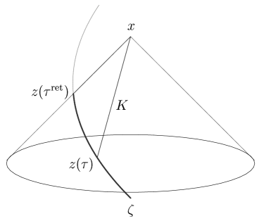
Figure 1: In four dimensions the retarded potential at field point $x$ is generated by a single event in space-time: the intersection $z(\tau^{\rm ret})$ of the world line $\zeta$ and $x$’s past light cone. In three dimensions the retarded potential depends on the segment of $\zeta$ that corresponds to time interval $]-\infty,\tau^{\rm ret}(x)]$. The vector $K$ is a vector pointing from the emission point $z(\tau)\in\zeta$ to field point $x$.

Convolving the retarded Green function (4.1) with charge-current density (4.2), we construct the retarded Liénard-Wiechert potential in three dimensions:

$$A_{\mu}^{\rm ret}(x)=e\int_{-\infty}^{\tau^{\rm ret}(x)}{\rm d}\tau\frac{u_{\mu}(\tau)}{\sqrt{-(K\cdot K)}}.$$ (4.3)

It is generated by the point charge during its entire past history before the retarded time $\tau^{\rm ret}(x)$ associated with the field point $x$ (see figure 1). We denote $K^{\mu}=x^{\mu}-z^{\mu}(\tau)$ the unique timelike (or null) vector connecting a field point $x$ to the emission point $z(\tau)\in\zeta$. The dot denotes the scalar product of three-vector $K$ on itself. $(K\cdot K)$ is equal to double Synge’s function $\sigma(x,z(\tau))$ of field point $x$ and emission point $z(\tau)$.

The simplest potential is produced by an unmoved charge placed at the coordinate origin. The world line $\zeta$ is given by $z^{\mu}=(t,0,0)$. The retarded instant $\tau^{\rm ret}(x)=x^{0}-r$ where $r:=\sqrt{(x^{1})^{2}+(x^{2})^{2}}$ is distance from the field point with coordinates $(x^{0},x^{1},x^{2})$ to the charge. Since 3-velocity $u_{\mu}=(-1,0,0)$, the only nontrivial components of the retarded potential (4.3) is

$$A_{0}^{\rm ret} = e\int_{-\infty}^{x^{0}-r}{\rm d}t\frac{-1}{\sqrt{(x^{0}-t)^{2}-r^{2}}}$$

$$= \left.-e\ln\left(x^{0}-t-\sqrt{(x^{0}-t)^{2}-r^{2}}\right)\right|_{t\to-\infty}^{t=x^{0}-r}$$

$$= -e\ln r.$$

Having used metric tensor $\eta^{\alpha\beta}={\rm diag}(-1,1,1)$ to raise index, we arrive at the logarithmic static potential

$$A^{0}_{\rm ret}=e\ln r.$$

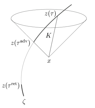
Figure 2: The portion of the world line after $\tau^{\rm adv}(x)$ produces the advanced potential in three dimensions. Advanced instant labels point at which particle’s world line punctures future light cone with vertex at field point $x$. Retarded instant $\tau^{\rm ret}(x)$ associated with point $x$ is before the moment $\tau^{\rm adv}(x)$.

The advanced Green’s function

$$G_{2+1}^{\rm adv}(x,y)=\frac{\theta(-x^{0}+y^{0}+|{\mathbf{x}}-{\mathbf{y}}|)}{\sqrt{-2\sigma(x,y)}}.$$

is nonzero in the past of the emission point $y$. Convolving it with charge-current density (4.2), we construct the advanced potential:

$$A_{\mu}^{\rm adv}(x)=e\int^{+\infty}_{\tau^{\rm adv}(x)}{\rm d}\tau\frac{u_{\mu}(\tau)}{\sqrt{-(K\cdot K)}}.$$

It is generated by the point charge during its entire future history following the advanced time $\tau^{\rm adv}(x)$ (see figure 2).

Static advanced potential coincides with the retarded one.

5 Electromagnetic field in 2+1 electrodynamics

The field $F_{\mu\nu}^{\rm ret}=\partial_{\mu}A^{\rm ret}_{\nu}-\partial_{\nu}A^{\rm ret}_{\mu}$ consists of two quite different terms. The first term is due to dependence of the upper limit in path integral (4.3) on field point $x$:

$$F_{\mu\nu}^{(\delta)}=\lim_{\tau\to\tau^{\rm ret}}\frac{e}{\sqrt{-(K\cdot K)}}\frac{u_{\mu}K_{\nu}-u_{\nu}K_{\mu}}{-(K\cdot u)}.$$ (5.1)

We take into account that

$$\frac{\partial\tau^{\rm ret}(x)}{\partial x^{\mu}}=-k_{\mu},$$

where $k_{\mu}=K_{\mu}/r,r=-(K\cdot u)$. Since $\tau^{\rm ret}(x)$ is the root of algebraic equation

$$(K\cdot K) = \eta_{\alpha\beta}(x^{\alpha}-z^{\alpha}(\tau))(x^{\beta}-z^{\beta}(\tau))$$

$$= 0,$$

direct term ${\hat{F}}^{(\delta)}$ diverges.

The second term

$$F_{\mu\nu}^{(\theta)}=-e\int_{-\infty}^{\tau^{\rm ret}(x)}d\tau\frac{u_{\mu}K_{\nu}-u_{\nu}K_{\mu}}{[-(K\cdot K)]^{3/2}}$$ (5.2)

arises from differentiation of expression under the integral sign in eq.(4.3).

The direct part (5.1), which depends on the momentary characteristics of the charge, and the tail part (5.2), which depends on its previous evolution, separately diverge on the light cone. The singularity, however, can be removed from the sum of ${\hat{F}}^{(\delta)}$ and ${\hat{F}}^{(\theta)}$. Using the identity

$$\frac{1}{[-(K\cdot K)]^{3/2}}=\frac{1}{-(K\cdot u)}\frac{\rm d}{{\rm d}\tau}\frac{1}{\sqrt{-(K\cdot K)}}$$

in eq.(5.2) yields

$$F_{\mu\nu}^{(\theta)} = -\frac{e}{\sqrt{-(K\cdot K)}}\left.\frac{u_{\mu}K_{\nu}-u_{\nu}K_{\mu}}{-(K\cdot u)}\right|_{\tau\to-\infty}^{\tau\to\tau^{\rm ret}(x)}$$

$$+ e\int_{-\infty}^{\tau^{\rm ret}(x)}\frac{{\rm d}\tau}{\sqrt{-(K\cdot K)}}\left\{\frac{u_{\mu}K_{\nu}-u_{\nu}K_{\mu}}{[-(K\cdot u)]^{2}}\left[1+(K\cdot a)\right]+\frac{a_{\mu}K_{\nu}-a_{\nu}K_{\mu}}{-(K\cdot u)}\right\}$$

after integration by parts. Summing up (5.1) and (5) and taking into account that $1/\sqrt{-(K\cdot K)}$ vanishes whenever $\tau\to-\infty$, we finally obtain the expression

$${\hat{F}}^{\rm ret}(x)=e\int_{-\infty}^{\tau^{\rm ret}(x)}\frac{{\rm d}\tau}{\sqrt{-(K\cdot K)}}\left\{\frac{u\wedge K}{r^{2}}\left[1+(K\cdot a)\right]+\frac{a\wedge K}{r}\right\},$$ (5.4)

which is regular on the light cone. (It diverges on the particle’s trajectory only where field point $x$ approaches emission point $z\in\zeta$.) Symbol $\wedge$ denotes the wedge product. The invariant quantity

$$r = -(K\cdot u)$$

$$= -\eta_{\alpha\beta}(x^{\alpha}-z^{\alpha}(\tau))u^{\beta}(\tau)$$

is an affine parameter on the time-like (null) geodesic that links $x$ to $z(\tau)$; it can be loosely interpreted as the time delay between $x$ and $z(\tau)$ as measured by an observer moving with the particle. Because the speed of light is set to unity, parameter $r(\tau^{\rm ret})$ is also the spatial distance between $z(\tau^{\rm ret})$ and $x$ as measured in this momentarily comoving Lorentz frame.

Calculation of the advanced strength tensor

$${\hat{F}}^{\rm adv}(x)=e\int^{+\infty}_{\tau^{\rm adv}(x)}\frac{{\rm d}\tau}{\sqrt{-(K\cdot K)}}\left\{\frac{a\wedge K}{r}+\frac{u\wedge K}{r^{2}}\left[1+(K\cdot a)\right]\right\}$$

is identical to that of the retarded one and we do not bother with details. Advanced field is generated by the point charge during its entire future history following the advanced time associated with $x$ (see figure 2).

6 Field of a uniformly moving charge

To calculate the electromagnetic field generated by a uniformly moving charge we substitute the functions which parameterize the straightforward world line

$$z^{\mu}(\tau)=z^{\mu}_{0}+u^{\mu}\tau$$

in eq.(5.4). We split the vector $K^{\mu}=x^{\mu}-z^{\mu}(\tau)$ into constant vector $K^{\mu}_{0}=x^{\mu}-z^{\mu}_{0}$ and time-dependent part:

$$K^{\mu}=K^{\mu}_{0}-u^{\mu}\tau.$$

The square of this 3-vector is quadratic in proper time $\tau$:

$$-(K\cdot K)=\tau^{2}+2(K_{0}\cdot u)\tau-(K_{0}\cdot K_{0}).$$

The retarded instant

$$\tau^{\rm ret}(x)=-(K_{0}\cdot u)-\sqrt{(K_{0}\cdot u)^{2}+(K_{0}\cdot K_{0})}$$

and the advanced one

$$\tau^{\rm adv}(x)=-(K_{0}\cdot u)+\sqrt{(K_{0}\cdot u)^{2}+(K_{0}\cdot K_{0})}$$

satisfy the light cone equation $(K\cdot K)=0$.

Since particle’s acceleration vanishes and the wedge product $u\wedge K=u\wedge K_{0}$ does not depend on time, the retarded field (5.4) looks relatively simple:

$${\hat{F}}^{\rm ret}(x) = e\int_{-\infty}^{\tau^{\rm ret}(x)}\frac{{\rm d}\tau}{\sqrt{[\tau+(K_{0}\cdot u)]^{2}-(K_{0}\cdot u)^{2}-(K_{0}\cdot K_{0})}}\frac{u\wedge K_{0}}{[-(K_{0}\cdot u)-\tau]^{2}}$$ (6.1)

$$= \left.-e\frac{u\wedge K_{0}}{(K_{0}\cdot u)^{2}+(K_{0}\cdot K_{0})}\sqrt{1-\frac{(K_{0}\cdot u)^{2}+(K_{0}\cdot K_{0})}{[-(K_{0}\cdot u)-\tau]^{2}}}\right|_{\tau\to-\infty}^{\tau=\tau^{\rm ret}(x)}$$

$$= e\frac{u\wedge K_{0}}{(K_{0}\cdot u)^{2}+(K_{0}\cdot K_{0})}.$$

Taking into account that the denominator is the square of the retarded distance (5) and substituting $u\wedge K$ for $u\wedge K_{0}$, we finally obtain

$${\hat{F}}^{\rm ret}(x)=e\frac{u\wedge K}{r_{\rm ret}^{2}}.$$ (6.2)

Can the uniformly moving charge “fill” this field? To answer this question we place the field point $x$ on particle’s world line: $x^{\mu}=z_{0}^{\mu}+u^{\mu}\tau_{x}$. In such a case the separation vector $K^{\mu}=u^{\mu}(\tau_{x}-\tau)$ is collinear with particle’s velocity. The strength tensor (6.2) vanishes on $\zeta$ and, therefore, the uniformly moving charge can not be accelerated due to its own field.

The simplest field is generated by a static charge placed at the coordinate origin. Setting $z=(t,0,0)$ and $u=(1,0,0)$ in eq.(6.1), one can derive that the only nontrivial components of static field are:

$$F_{i0} = e\int\limits_{-\infty}^{x^{0}-r}\frac{{\rm d}t}{\sqrt{(x^{0}-t)^{2}-r^{2}}}\frac{x^{i}}{(x^{0}-t)^{2}}$$

$$= \left.-e\frac{x^{i}}{r^{2}}\frac{\sqrt{(x^{0}-t)^{2}-r^{2}}}{x^{0}-t}\right|_{t\to-\infty}^{t=x^{0}-r}=e\frac{x^{i}}{r^{2}}.$$

$r:=\sqrt{(x^{1})^{2}+(x^{2})^{2}}$ is the distance to the charge. Since (2.3), $F_{10}=E^{1}$ and $F_{20}=E^{2}$; magnetic component $H=0$.

An interaction between two static charges, say $e_{1}$ and $e_{2}$, is caused by the Lorentz force $F^{\alpha}_{ab}=e_{a}u_{a}^{\beta}F^{\alpha}{}_{\beta}$. Electric field (6) of the unmoved charge yields the stronger electrostatic force in comparison with its counterpart in conventional electrodynamics:

$${\mathbf{F}}_{ab}=e_{1}e_{2}\frac{{\mathbf{n}}_{r}}{r}.$$

Unit vector ${\mathbf{n}}_{r}:=({\mathbf{z}}_{a}-{\mathbf{z}}_{b})/r,r=|{\mathbf{z}}_{1}-{\mathbf{z}}_{2}|$ is the distance between charges; ${\mathbf{z}}_{a}$ is position 2-vector of $a$-th charge. The magnitude of the electrostatic force between two point charge is directly proportional to the magnitudes of each charge and inversely proportional to the distance between the charges.

Coulomb’s law in three dimensions is similar to that in conventional spacetime of four dimensions. What is happen when the first clamp releases the charge? In four dimensions $e_{1}$ moves in electrostatic field of charge $e_{2}$. While in three dimensions the accelerated charge is influenced by its own field too! So, the “static” segment of the world line $\zeta_{1}$ generates the field

$$F_{i0} = e_{1}\int\limits_{-\infty}^{0}\frac{{\rm d}t}{\sqrt{(x^{0}-t)^{2}-r^{2}}}\frac{x^{i}}{(x^{0}-t)^{2}}$$

$$= \left.-e_{1}\frac{x^{i}}{r^{2}}\frac{\sqrt{(x^{0}-t)^{2}-r^{2}}}{x^{0}-t}\right|_{t\to-\infty}^{t=0}$$

$$= e_{1}\frac{x^{i}}{r^{2}}\left(1-\sqrt{1-\frac{r^{2}}{(x^{0})^{2}}}\right).$$

Curvilinear segment of $\zeta_{1}$ (it corresponds to the time interval after initial instant $t=0$ when the charge becomes free) acts on $e_{1}$ too. The situation looks like a charge “repulses” itself taken in future instant of time. The “self-force” is inversely proportional to the distance between the “momentary” charge and the same charge taken at previous instant of time. What is happen when the points on the world line are very close?

To answer this question we evaluate the “Lorentz self-force density”

$$f^{\mu}_{\rm ret}(\tau,s) = \frac{e^{2}}{\sqrt{-(q\cdot q)}}\left\{\frac{u_{s}^{\mu}(u_{\tau}\cdot q)-(u_{\tau}\cdot u_{s})q^{\mu}}{r_{s}^{2}}\left[1+(q\cdot a_{s})\right]\right.$$

$$+ \left.\frac{a_{s}^{\mu}(u_{\tau}\cdot q)-(u_{\tau}\cdot a_{s})q^{\mu}}{r_{s}}\right\},$$

in the $s\to\tau$ limit. (Expression (6) is the contraction of the integrand of eq.(5.4) where field point $x=z(\tau)\in\zeta$, with particle’s velocity $u(\tau)$.) Index $\tau$ indicates that the particle’s velocity or position is referred to the actual instant $\tau$ while index $s$ says that the particle’s characteristics are evaluated at previous instant $s<\tau$. Since both the field point $x=z(\tau)$ and the point of emission $z(s)$ lie on the same world line, the separation vector $K$ becomes $q(\tau,s)=z_{\tau}-z_{s}$; $r_{s}=-(q\cdot u_{s})$. With a degree of accuracy sufficient for our purposes

$$\sqrt{-(q\cdot q)} = \Delta,$$

$$q^{\mu} = \Delta\left[u_{\tau}^{\mu}-a_{\tau}^{\mu}\frac{\Delta}{2}+{\dot{a}}_{\tau}^{\mu}\frac{\Delta^{2}}{6}\right],$$

$$u_{s}^{\mu} = u_{\tau}^{\mu}-a_{\tau}^{\mu}\Delta+{\dot{a}}_{\tau}^{\mu}\frac{\Delta^{2}}{2},$$

$$a_{s}^{\mu} = a_{\tau}^{\mu}-{\dot{a}}_{\tau}^{\mu}\Delta,$$

where $\Delta=\tau-s$ is positive small parameter. Substituting these into integrand of the double integral of eq. (6) and passing to the limit $\Delta\to 0$ yields diverging expression:

$$\lim_{s\to\tau}f^{\mu}_{\rm ret}(\tau,s)=-\frac{e^{2}}{2}\lim_{\Delta\to 0}\frac{a^{\mu}_{\tau}}{\Delta}+\frac{2e^{2}}{3}\left({\dot{a}}_{\tau}^{\mu}-a_{\tau}^{2}u_{\tau}^{\mu}\right).$$ (6.5)

Whence the “Lorentz self-force” $\int_{-\infty}^{\tau}f^{\mu}_{\rm ret}(\tau,s)$ can not be thought as the self-action in $2+1$ electrodynamics and the renormalization procedure is necessary.

7 Regularization procedure

The main idea ought to be straightforward to formulate: the retarded field carries energy-momentum and angular momentum; outgoing waves remove energy, momentum, and angular momentum from the source which then undergoes a radiation reaction. Unfortunately, the problem is ambiguous since the field diverges in the neighbourhood of the particle’s world line. A rule is necessary for extracting the appropriate finite parts of Noether quantities which exert the radiation reaction.

The flow of energy-momentum that flows across a space-like surface $\Sigma$ is given by the integral [20]

$$p^{\nu}_{\rm em}(\tau)=\int_{\Sigma}{\rm d}\sigma_{\mu}T^{\mu\nu},$$ (7.1)

of the Maxwell energy-momentum tensor density

$$2\pi T^{\mu\nu}=F^{\mu\lambda}F^{\nu}{}_{\lambda}-1/4\eta^{\mu\nu}F^{\kappa\lambda}F_{\kappa\lambda}.$$ (7.2)

over $\Sigma$. Since Huygens principle does not hold in three dimensions (see Figure 3) and field (5.4) develops a tail, the integration means the study of interference of outgoing electromagnetic waves emitted by different points on $\zeta$.

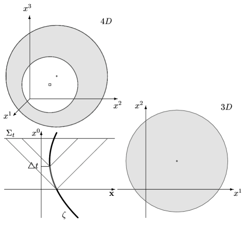
Figure 3: Let the point source radiates within the interval $[0,\triangle t]$. In four dimensions the support of the Maxwell energy-momentum tensor density in hyperplane $x^{0}=t$ is in between two spheres centered at points $z^{i}(0)$ (cross symbol) and $z^{i}(\triangle t)$ (box symbol) with radii $t$ and $t-\triangle t$, respectively. If the interval is infinitesimal, the support becomes two-dimensional sphere. In three dimensions the radiation fills the disk with radius $t$ centered at point $z^{i}(0)$ (cross symbol) even if the interval shrinks to zero.

To calculate the flow of energy-momentum (7.1), an appropriate surface of integration $\Sigma$ is necessary. The tilted hyperplane which plays privileged role in the one-particle radiation reaction problem in four dimensions [15] is not suitable whenever the self-action problem in three dimensions is considered. The reason is that the amount of radiated energy-momentum in $\Sigma$ depends on all previous evolution of a source. There is no a plane which is orthogonal to the particle’s 3-velocities at all points on $\zeta$ before the end point $z(\tau)=\zeta\cap\Sigma$. We choose the simplest plane $\Sigma_{t}=\{x\in{\mathbb{M}}_{\,3}:x^{0}=t\}$ associated with an unmoving inertial observer. Non-covariant terms arise unavoidable due to integration over this surface. To reveal meaningful contribution in radiated energy-momentum we apply the criteria which were first formulated in [15, Table 1]:

• the bound term diverges while the radiative one is finite;

• the bound component depends on the momentary state of the particle’s motion while the radiative one is accumulated with time; and

• the form of the bound terms heavily depends on choosing of an integration surface while the radiative terms are invariant.

The second point should be define more accurately. In conventional electrodynamics the bound contribution (Shott term) depends on the momentary state of particle’s motion while the radiated energy-momentum carried by electromagnetic field is the path integral of Larmor expression. In three dimensions both the bound term and the radiative one develop tails. But the radiative terms have one extra path integration in comparison with the bound ones.

The bound parts of Noether quantities modify particle’s individual characteristics (its mass, its momentum and its angular momentum). To establish tail field contribution into particle’s individual characteristics we do not manipulate with divergent non-covariant bound terms. We did not make any assumptions about the particle structure, its charge distribution, and its size. We only assume that the momentum of dressed charge is finite. To obtain additional information we calculate the flow of angular momentum [20]

$$M_{\rm em}^{\mu\nu}(t)=\int_{\Sigma_{t}}{\rm d}\sigma_{0}\left(x^{\mu}T^{0\nu}-x^{\nu}T^{0\mu}\right)$$ (7.3)

which flows across $\Sigma_{t}=\{x\in{\mathbb{M}}_{\,3}:x^{0}=t\}$. To reveal radiative part of ${\hat{M}}_{\rm em}$ we apply Teitelboim’s criteria. Further we assume that the bound terms are absorbed by particle’s individual characteristics within the renormalization procedure while the radiative terms survive and lead an independent existence. The change in radiative energy-momentum and angular momentum carried by the electromagnetic field should be balanced by a corresponding change of particle’s momentum and angular momentum, respectively. Analysis of six balance equations gives the form of individual characteristics of dressed charged particle as well as effective equation of motion which includes effect of particle’s own field.

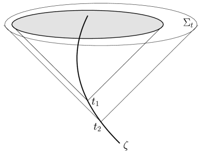
Figure 4: Outgoing electromagnetic waves generated by the portion of the world line that corresponds to the interval $-\infty<t_{2}<t_{1}$ combine within the gray disk in the plane $\Sigma_{t}$. It is centered at point with coordinates $(z^{1}(t_{1}),z^{2}(t_{1}))$. Corresponding domain of integration is $\int_{-\infty}^{\tau}{\rm d}t_{1}\int_{-\infty}^{t_{1}}{\rm d}t_{2}\int_{0}^{k_{1}^{0}}{\rm d}R\int_{0}^{2\pi}{\rm d}\varphi$ where $k_{1}^{0}$ is the radius of smaller disk.

7.1 Radiated energy-momentum of electromagnetic field

Figure 4 pictures the interference of waves generated by fixed point $z(t_{1})\in\zeta$ with radiation produced by charge before $t_{1}$. It is convenient to parametrize the plane $x^{0}=t$ by circular coordinates $R$ and $\varphi$. Since the stress-energy tensor (7.2) is quadratic in field strengths, we should twice integrate it over $\zeta$. The amount of radiated energy-momentum is given by fourfold integral

$$p_{\rm R}^{\nu}=\int\limits_{-\infty}^{t}{\rm d}t_{1}\int\limits_{-\infty}^{t_{1}}{\rm d}t_{2}\int\limits_{0}^{k_{1}^{0}}{\rm d}R\int\limits_{0}^{2\pi}{\rm d}\varphi Jt^{0\nu}_{12},$$ (7.4)

where $J$ is Jakobian of coordinate transformation [16, eq.(4.5)]. The integrand

$$2\pi t^{\alpha\beta}_{12}=f_{(1)}^{\alpha\lambda}f_{(2)\lambda}^{\beta}-\frac{1}{4}\eta^{\alpha\beta}f_{(1)}^{\mu\nu}f^{(2)}_{\mu\nu}$$ (7.5)

describes the combination of field strength densities at $x\in\Sigma_{t}$

$$f_{\mu\nu}=\frac{e}{\sqrt{-(K\cdot K)}}\left\{\frac{u_{\mu}K_{\nu}-u_{\nu}K_{\mu}}{[-(K\cdot u)]^{2}}\left[1+(K\cdot a)\right]+\frac{a_{\mu}K_{\nu}-a_{\nu}K_{\mu}}{-(K\cdot u)}\right\},$$

generated by emission points $z(t_{1})\in\zeta$ and $z(t_{2})\in\zeta$.

The calculation is performed in Ref.[16] where radiative terms are extracted. Resulting expressions can be rewritten in a manifestly covariant fashion when the world line is parameterized by a proper time $\tau$. The fourfold integral (7.4) contributes in radiated energy-momentum one-half of the work

$$p_{\rm R}^{\mu}=-\frac{1}{2}\int_{-\infty}^{\tau}{\rm d}\tau_{1}F_{\rm ret}^{\mu}(\tau_{1}),$$

of the retarded tail Lorentz force

$$F_{\rm ret}^{\mu}(\tau_{1}) = eF_{(\theta)}^{\mu\alpha}u_{1,\alpha}$$

$$= e^{2}\int_{-\infty}^{\tau_{1}}{\rm d}\tau_{2}\frac{-(q\cdot u_{1})u_{2}^{\mu}+(u_{1}\cdot u_{2})q^{\mu}}{[-(q\cdot q)]^{3/2}},$$

taken with opposite sign.

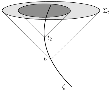
Figure 5: Outgoing electromagnetic waves generated by the portion of the world line that corresponds to the interval $t_{1}<t_{2}\leq t$ joint together inside the dark disk. It is centered at point with coordinates $(z^{1}(t_{2}),z^{2}(t_{2}))$. The domain of integration becomes $\int_{-\infty}^{t}{\rm d}t_{1}\int^{t}_{t_{1}}{\rm d}t_{2}\int_{0}^{k_{2}^{0}}{\rm d}R\int_{0}^{2\pi}{\rm d}\varphi$ where $k_{2}^{0}$ is the radius of dark disk.

Figure 5 illustrates the interference of the radiation emanated by fixed point $z(t_{1})\in\zeta$ with waves generated by charge during the interval $[t_{1},t]$. The portion of energy-momentum produced by this segment of $\zeta$ is given by the multiple integral

$$p_{\rm A}^{\nu}=\int\limits_{-\infty}^{t}{\rm d}t_{1}\int\limits^{t}_{t_{1}}{\rm d}t_{2}\int\limits_{0}^{k_{2}^{0}}{\rm d}R\int\limits_{0}^{2\pi}{\rm d}\varphi Jt^{0\nu}_{12},$$

where tensor $t^{0\nu}_{12}$ is defined by eq.(7.5). This fourfold integral contributes in radiated energy-momentum one-half of work

$$p_{\rm A}^{\mu}=-\frac{1}{2}\int_{-\infty}^{\tau}{\rm d}\tau_{1}F_{\rm adv}^{\mu}(\tau_{1}),$$

of the advanced tail Lorentz force

$$F_{\rm adv}^{\mu}(\tau_{1})=e^{2}\int^{\tau}_{\tau_{1}}{\rm d}\tau_{2}\frac{-(q\cdot u_{1})u_{2}^{\mu}+(u_{1}\cdot u_{2})q^{\mu}}{[-(q\cdot q)]^{3/2}},$$ (7.7)

that differs from its retarded counterpart (7.1) by the domain of integration only.

The radiative part of energy-momentum carried by electromagnetic field is therefore

$$p_{\rm rad}^{\mu}(\tau)=-\frac{1}{2}\int_{-\infty}^{\tau}{\rm d}\tau_{1}\left(F_{\rm ret}^{\mu}-F_{\rm adv}^{\mu}\right).$$ (7.8)

The resulting expression obeys the spirit of Dirac’s decomposition of the retarded electromagnetic field into the “mean of the advanced and retarded field” and the “radiation” field. The situation is pictured in Figure 6.

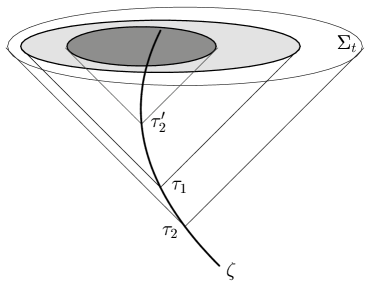
Figure 6: We call “retarded” the force (7.1) with integration over the portion of the world line before $\tau_{1}$. We call “advanced” the force (7.7) with integration over the portion of the world line after $\tau_{1}$. For an observer placed at point $z(\tau_{1})\in\zeta$ the regular radiative part (7.8) of electromagnetic field momentum looks as the combination of incoming and outgoing radiation. And yet the retarded causality is not violated. We still consider the interference of outgoing waves presented at the observation instant $\tau$. The electromagnetic field carries information about the charge’s past.

7.2 Radiated angular momentum of electromagnetic field

Surface integration of the torque of the stress-energy tensor (7.3) is identical to that of the energy and momentum tensor densities. Details of computations is presented in ref.[16]. The amount of radiated angular momentum that corresponds to interference pictured in figure 4 is as follows:

$$M_{\rm ret}^{\mu\nu}=-\frac{1}{2}\int_{-\infty}^{\tau}{\rm d}\tau_{1}\left[z_{1}^{\mu}F_{\rm ret}^{\nu}(\tau_{1})-z_{1}^{\nu}F_{\rm ret}^{\mu}(\tau_{1})\right].$$

It is then nothing but one-half of the path integral of the torque of tail Lorentz force (7.1). Combination of waves pictured in figure 5 contributes in radiated angular momentum one-half of the path integral of the torque of “advanced” Lorentz force (7.7):

$$M_{\rm adv}^{\mu\nu}=-\frac{1}{2}\int_{-\infty}^{\tau}{\rm d}\tau_{1}\left[z_{1}^{\mu}F_{\rm adv}^{\nu}(\tau_{1})-z_{1}^{\nu}F_{\rm adv}^{\mu}(\tau_{1})\right].$$

Total angular momentum which leads an independent existence and can be detected by distant devices is as follows:

$$M_{\rm rad}^{\mu\nu}(\tau) = -\frac{1}{2}\int_{-\infty}^{\tau}{\rm d}\tau_{1}\left(M_{\rm ret}^{\mu\nu}-M_{\rm adv}^{\mu\nu}\right)$$

$$= -\frac{1}{2}\int_{-\infty}^{\tau}{\rm d}\tau_{1}\left[z_{1}^{\mu}\left(F_{\rm ret}^{\nu}-F_{\rm adv}^{\nu}\right)-z_{1}^{\nu}\left(F_{\rm ret}^{\mu}-F_{\rm adv}^{\mu}\right)\right].$$

Together with radiated energy-momentum (7.8), it exert the radiation reaction.

8 Equation of motion of radiating charge

We therefore introduce the radiative part (7.8) of energy-momentum and postulate that it, and it alone, exerts a force on the particle. Singular part should be coupled with particle’s three-momentum, so that “dressed” charged particle would not undergo any additional radiation reaction. Already renormalized particle’s individual three-momentum, say $p_{\rm part}$, together with $p_{\rm rad}$ constitute the total energy-momentum of our composite particle plus field system: $P=p_{\rm part}+p_{\rm rad}$.

The total angular momentum, say $\hat{M}$, consists of particle’s angular momentum $z\wedge p_{\rm part}$ and radiative part (7.2) of angular momentum carried by electromagnetic field:

$$M^{\mu\nu}=z_{\tau}^{\mu}p_{\rm part}^{\nu}(\tau)-z_{\tau}^{\nu}p_{\rm part}^{\mu}(\tau)+M^{\mu\nu}_{\rm rad}(\tau).$$

The one-half sum of the retarded and the advanced works is the bound part of tail energy-momentum which is permanently attached to the charge and is carried along with it. It modifies particle’s individual characteristics (its momentum and its inertial mass). A point source together with surrounded electromagnetic “cloud” constitute new entity: dressed charged particle.

Balance equations ${\dot{P}}=F_{\rm ext}$ and ${\dot{M}}=z_{\tau}\wedge F_{\rm ext}$ result integro-differential equation of motion of a dressed charged particle in an external field

$$ma^{\mu}_{\tau}=eu_{\tau,\alpha}F^{\mu\alpha}_{\rm ret}(\tau)+\frac{e^{2}}{2}a^{\mu}_{\tau}\int_{-\infty}^{\tau}\frac{{\rm d}s}{\sqrt{-(q\cdot q)}}+eu_{\tau,\alpha}F^{\mu\alpha}_{\rm ext},$$ (8.1)

where the radiation reaction is taken into account. The non-local term in equation (8.1) which is proportional to particle’s acceleration $a(\tau)$ arises also in [19]. It provides proper short-distance behavior of the perturbations due to the particle’s own field. If $s\to\tau$ the integrand tends to three-dimensional analog of the Abraham radiation reaction vector:

$$\lim_{s\to\tau}\left[eu_{\tau,\alpha}f^{\mu\alpha}(\tau,s)+\frac{e^{2}}{2}\frac{a^{\mu}_{\tau}}{\sqrt{-(q\cdot q)}}\right]=\frac{2}{3}e^{2}\left({\dot{a}}^{\mu}-a^{2}u^{\mu}\right),$$

cf. eq.(6.5). All quantities on the right-hand side refer to the instant of observation $\tau$.

Individual 3-momentum of a dressed charged particle contains nonlocal contribution from tail electromagnetic field of the particle:

$$p_{\rm part}^{\mu}(\tau)=mu^{\mu}(\tau)+\frac{e^{2}}{2}\int_{-\infty}^{\tau}{\rm d}s\frac{u^{\mu}(s)-u^{\mu}(\tau)}{\sqrt{-(q\cdot q)}}.$$

The balance equations produces also a time-changing inertial mass:

$$\dot{m}=\frac{e^{2}}{2}\int_{-\infty}^{\tau}{\rm d}s\frac{(q\cdot u_{\tau})-(q\cdot u_{s})}{[-(q\cdot q)]^{3/2}}.$$ (8.2)

It is interesting that similar phenomenon occurs in the theory which describes a point-like charge coupled with massless scalar field in flat spacetime of three dimensions [21]. The charge loses its mass through the emission of monopole radiation.

9 Radiating charge in uniform static electric field

Let us consider a constant electromagnetic field with components

$$\left(F^{\mu\nu}_{\rm ext}\right)=\left(\begin{array}[]{ccc}0&E&0\\ -E&0&0\\ 0&0&0\end{array}\right)$$

acting on the charge $e$ during the interval $[0,\tau_{0}]$. Before the initial instant $\tau=0$ the particle places at the coordinate origin.

If we neglect the self-action, the equation (8.1) becomes

$$\frac{{\rm d}u^{0}}{{\rm d}\tau}=\frac{e}{m}Eu^{1},\qquad\frac{{\rm d}u^{1}}{{\rm d}\tau}=\frac{e}{m}Eu^{0},\qquad\frac{{\rm d}u^{2}}{{\rm d}\tau}=0.$$

The test charge moves along hyperbola

$$z^{0}(\tau)=a^{-1}\sinh(a\tau),\qquad z^{1}(\tau)=a^{-1}\left[\cosh(a\tau)-1\right],\qquad z^{2}(\tau)=0,$$ (9.1)

where constant

$$a=\frac{e}{m}E$$

is the modulo of acceleration:

$$u^{0}(\tau) = \cosh(a\tau),\quad z^{1}(\tau)=\sinh(a\tau),\quad u^{2}(\tau)=0,$$ (9.2)

$$a^{0}(\tau) = a\sinh(a\tau),\quad z^{1}(\tau)=a\cosh(a\tau),\quad a^{2}(\tau)=0.$$

Let us suppose that external field is much more than electrostatic field generated by static segment of the world line, so that the radiation reaction does not change the type of particle’s world line. We substitute the solution (9.1) and its differential consequences (9.2) for corresponding quantities in the self-action terms of the equation of motion of radiating charge (8.1). So, the distance between charge at instant of observation $\tau<\tau_{0}$ and the same charge taken at moment $0<s<\tau$ depends on the difference $\tau-s$

$$\sqrt{-(q\cdot q)}=\frac{2}{a}\sinh[\frac{a}{2}(\tau-s)].$$

Hence the derivative of dynamical mass (8.2) vanishes.

It is of great importance that radiation back reaction is proportional to particle’s acceleration:

$$e^{2}\int_{0}^{\tau}{\rm d}s\left[u_{\alpha}(\tau)\frac{f^{\mu\alpha}(\tau,s)}{\sqrt{-(q\cdot q)}}+\frac{1}{2}\frac{a^{\mu}(\tau)}{\sqrt{-(q\cdot q)}}\right] = \left.\frac{e^{2}}{2}\frac{a^{\mu}(\tau)}{\cosh[a(\tau-s)/2]}\right|_{s=0}^{s=\tau}$$

$$= \frac{e^{2}}{2}a^{\mu}(\tau)\left[1-\frac{1}{\cosh(a\tau/2)}\right].$$

The portion of trajectory where the second term in between the square brackets is much less than $1$ approximates to hyperbola like (9.1) where modified mass $m-e^{2}/2$ should be substituted for $m$. The solution of the equation of motion (8.1) is given by functions (9.1) where new modulo of acceleration

$$a=\frac{eE}{m-e^{2}/2}$$

is greater than initial one. It is because the Lorentz self-force is repulsive (the charge interacts with itself).

After interaction zone, the charge fills the effect of radiation emitted by curvilinear portion of the world line. In general, the particle do not move uniformly nevermore. However, the contributions to the tail terms arising from portions of the trajectory distant to the current position of the particle should become negligible and its velocity will tend to a constant value.

10 Conclusions

In the present paper, we adopt the Dirac scheme of decomposition of the retarded Green’s function into symmetric (singular) and radiative (regular) parts to functions supported within light cones. The regularization scheme summarizes a scrupulous analysis of energy-momentum and angular momentum balance equations in $2+1$ electrodynamics [16, 17]. It differs from the approach developed by Detweiler and Whiting [9] on two “extra” entities: additional instant $\tau_{1}$ before the instant of observation and extra integration of the “half-difference” of the retarded and the advanced tail forces over particle’s path. So, the retarded tail force depends on the particle’s past history before $\tau_{1}<\tau$. Its advanced counterpart is generated by portion of the world line that corresponds to the interval $[\tau_{1},\tau]$. The tail part of radiated energy-momentum is one-half of the work done by the retarded force minus one-half of the work done by the advanced force, taken with opposite sign. This part of radiation detaches the point source and leads an independent existence.

The one-half sum of the retarded and the advanced works is the bound part of tail energy-momentum which is permanently attached to the charge and is carried along with it. It modifies particle’s individual characteristics (its momentum and its inertial mass).

Since the properties of the retarded and the advanced solutions of wave equation, the one-half sum is singular while one-half difference is regular in the immediate vicinity of the world line.

The items can be summarized as a simple scheme which obeys the spirit of Dirac’s scheme of decomposition of the retarded field in conventional electrodynamics into singular and regular parts. The main points are as follows.

• The tail retarded field can be decomposed into symmetric (singular) and radiative (regular) parts in standard Dirac’s manner.

• The support of both the retarded field and the advanced field is limited to particle’s world line.

The bound and the radiative angular momentum carried by charge’s field are simply torques of the above combinations of the retarded and the advanced tail forces.

Changes in individual momentum and angular momentum of dressed charged particle compensate losses of energy, momentum, and angular momentum due to radiation. (Influence of an external device can be modelled easily.) Analysis of balance equations gives the self-force and three-dimensional analogue of the Lorentz-Dirac equation.

References

- [1] S. Shankar, G. Sabouret, S.A.Lyon, J. Low Temp. Phys. 161, 410 (2010).
- [2] M. Boninsegni, J. Low Temp. Phys. 159, 441 (2010).
- [3] V.M. Loktev, M.D. Tomchenko, Ukr.J.Phys. 55, 901 (2010).
- [4] V.M. Loktev, M.D. Tomchenko, Phys.Rev.B 82, 172501 (2010).
- [5] L. Landau, J.Phys. USSR 5, 71 (1941).
- [6] L. Landau, J.Phys. USSR 11, 91 (1947).
- [7] R.J. Donnelly, Quantized vortices in Helium II (Cambridge University Press, Cambridge, 1991).
- [8] V. Ambegaokar, B.I. Halperin, D.R. Nelson, and E.D. Siggia, Phys. Rev. B 21, 1806 (1980).
- [9] S. Detweiler and B.F. Whiting, Phys. Rev. D 67, 024025 (2003).
- [10] P.A.M. Dirac, Proc. R. Soc. A (London) 167, 148 (1938).
- [11] B. S. DeWitt and R. W. Brehme, Ann.Phys. (N.Y.) 9, 220 (1960).
- [12] J. M. Hobbs, Ann.Phys. (N.Y.) 47, 141 (1968).
- [13] Y. Mino, M. Sasaki, and T. Tanaka, Phys. Rev. D 55, 3457 (1997).
- [14] T. C. Quinn, Phys. Rev. D 62, 064029 (2000).
- [15] C. Teitelboim, Phys. Rev. D 1, 1572 (1970).
- [16] Yu. Yaremko, J. Math. Phys. 48, 092901 (2007).
- [17] Yu. Yaremko, J.Phys.A: Math.Theor. 40, 13161 (2007).
- [18] D. V. Gal’tsov, Phys. Rev. D 66, 025016 (2002).
- [19] P. O. Kazinski, S. L. Lyakhovich, and A. A. Sharapov, Phys. Rev. D 66, 025017 (2002).
- [20] F. Rohrlich, Classical Charged Particles (Addison-Wesley, Redwood, CA, 1990).
- [21] L. M. Burko, Class. Quantum Grav. 19, 3745 (2002).